Download - complex variable PPT ( SEM 2 / CH -2 / GTU)

LD COLLEGE OF ENGINEERING
11. Complex Variable Theory
1. Complex Variables & Functions
2. Cauchy Reimann Conditions
3. Cauchy’s Integral Theorem
4. Cauchy’s Integral Formula
5. Laurent Expansion
6. Singularities
7. Calculus of Residues
8. Evaluation of Definite Inregrals
9. Evaluation of Sums
10. Miscellaneous Topics
Applications
1. Solutions to 2-D Laplace equation by means of conformal mapping.
2. Quantum mechanics.
3. Series expansions with analytic continuation.
4. Transformation between special functions, e.g., H (i x) c K (x) .
5. Contour integrals :a) Evaluate definite integrals & series.b) Invert power series.c) Form infinite products.d) Asymptotic solutions.e) Stability of oscillations.f) Invert integral transforms.
6. Generalization of real quantities to describe dissipation, e.g., Refraction index: n n + i k, Energy: E E + i
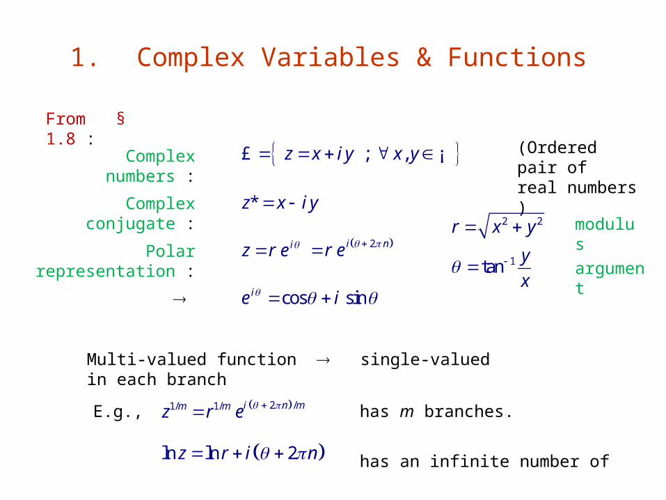
1. Complex Variables & Functions
; ,z x i y x y £ ¡Complex numbers : (Ordered pair of real numbers )
Complex conjugate : *z x i y
Polar representation : iz r e
2 2r x y modulus
1tan yx
argument
cos sinie i
From § 1.8 :
Multi-valued function single-valued in each branch
E.g., has m branches.
has an infinite number of branches.
2 /1/ 1/ i n mm mz r e
ln ln 2z r i n
2i nr e
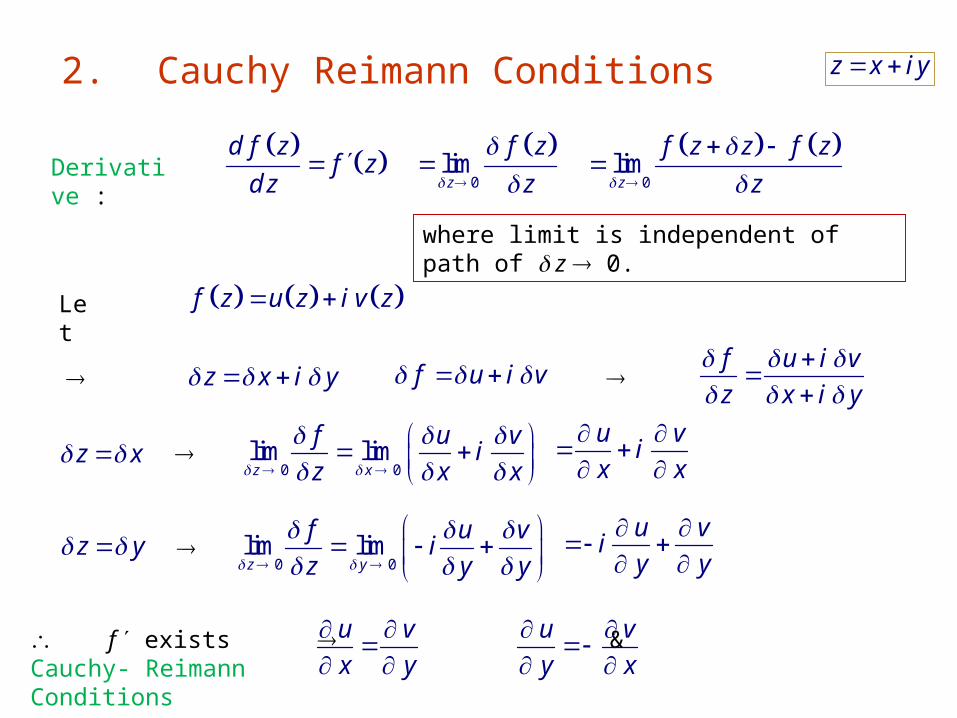
2. Cauchy Reimann Conditions
d f zf z
d zDerivative :
0
limz
f zz
0limz
f z z f zz
where limit is independent of path of z 0.
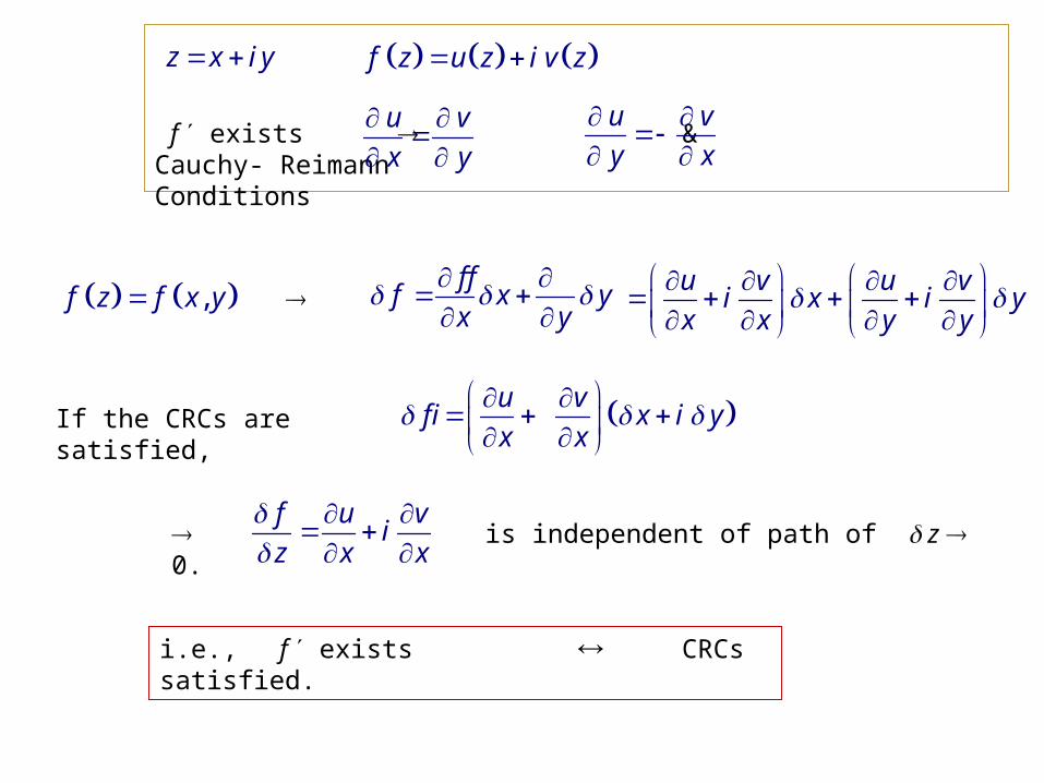
Let f z u z i v z
f u i v z x i y
f exists & Cauchy- Reimann Conditions
f u i vz x i y
z x 0 0
lim limz x
f u viz x x
u vix x
z y 0 0
lim limz y
f u viz y y
u viy y
u vx y
u vy x
z x i y
is independent of path of z 0.
f exists & Cauchy- Reimann
Conditions
u vx y
u vy x
If the CRCs are satisfied,
f z u z i v z z x i y
,f z f x y f ff x yx y
u v u vi x i yx x y y
u vf i x i yx x
f u viz x x
i.e., f exists CRCs satisfied.
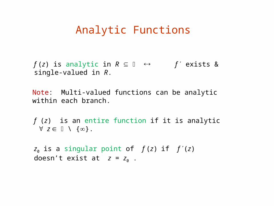
Analytic Functions
f (z) is analytic in R f exists & single-valued in R.
Note: Multi-valued functions can be analytic within each branch.
f (z) is an entire function if it is analytic z \ {}.
z0 is a singular point of f (z) if f (z) doesn’t exist at z = z0 .
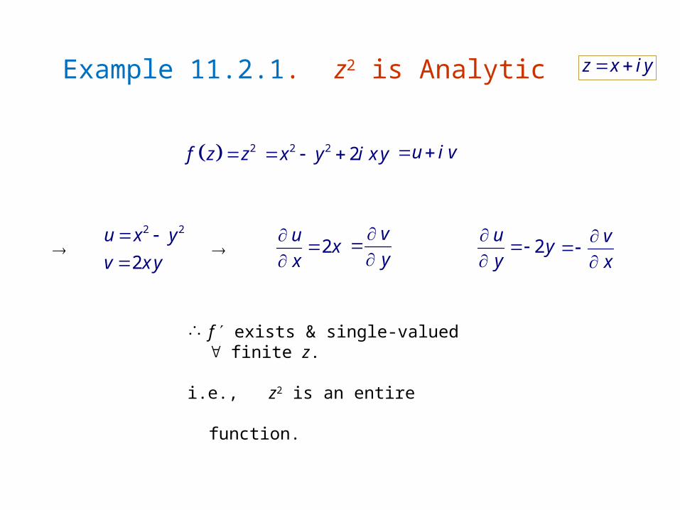
Example 11.2.1. z2 is Analytic
2f z z
z x i y
2 2 2x y i x y u i v
2 2
2u x yv x y
2u xx
vy
2u y
y
vx
f exists & single-valued finite z.
i.e., z2 is an entire function.
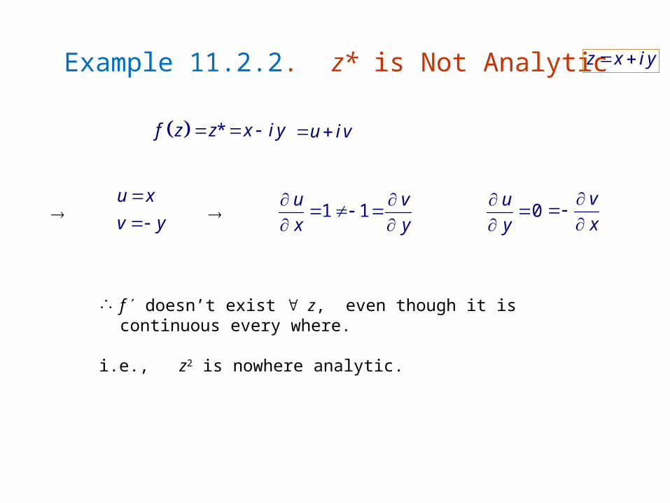
Example 11.2.2. z* is Not Analytic z x i y
*f z z x i y u i v
u xv y
1ux
1 vy
0u
y
vx
f doesn’t exist z, even though it is continuous every where.
i.e., z2 is nowhere analytic.
Harmonic Functions
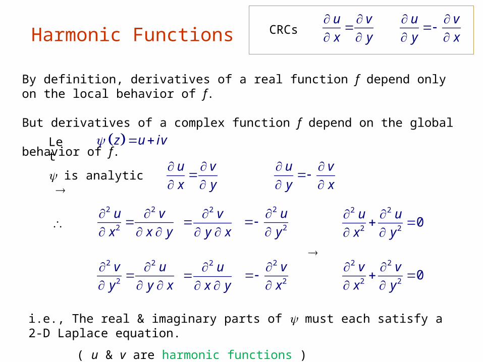
By definition, derivatives of a real function f depend only on the local behavior of f.
But derivatives of a complex function f depend on the global behavior of f.
u vx y
u vy x
CRCs
Let z u iv
is analytic u vx y
u vy x
2 2
2
u vx x y
2 vy x
2
2
uy
2 2
2
v uy y x
2 ux y
2
2
vx
2 2
2 2 0u ux y
2 2
2 2 0v vx y
i.e., The real & imaginary parts of must each satisfy a 2-D Laplace equation.
( u & v are harmonic functions )

u vx y
u vy x
CRCs
Contours of u & v are given by ,u x y c
0u udu d x d yx y
,v x y c
0v vd v d x d yx y
i.e., these 2 sets of contours are orthogonal to each other.
( u & v are complementary )
uu
ud y xm ud x
y
Thus, the slopes at each point of these contours are
vv
vd y xm vd x
y
CRCs at the intersections of these 2 sets of contours1u vm m

Derivatives of Analytic Functions
d f xg x
d x
Let f (z) be analytic around z, then
d f z
g zd z
Proof :
f (z) analytic f x i yf z
x
x z
d f xd x
g z
z x i y
E.g. 1n
nd x n xd x
1n
nd z n zd z
Analytic functions can be defined by Taylor series of the
same coefficients as their real counterparts.
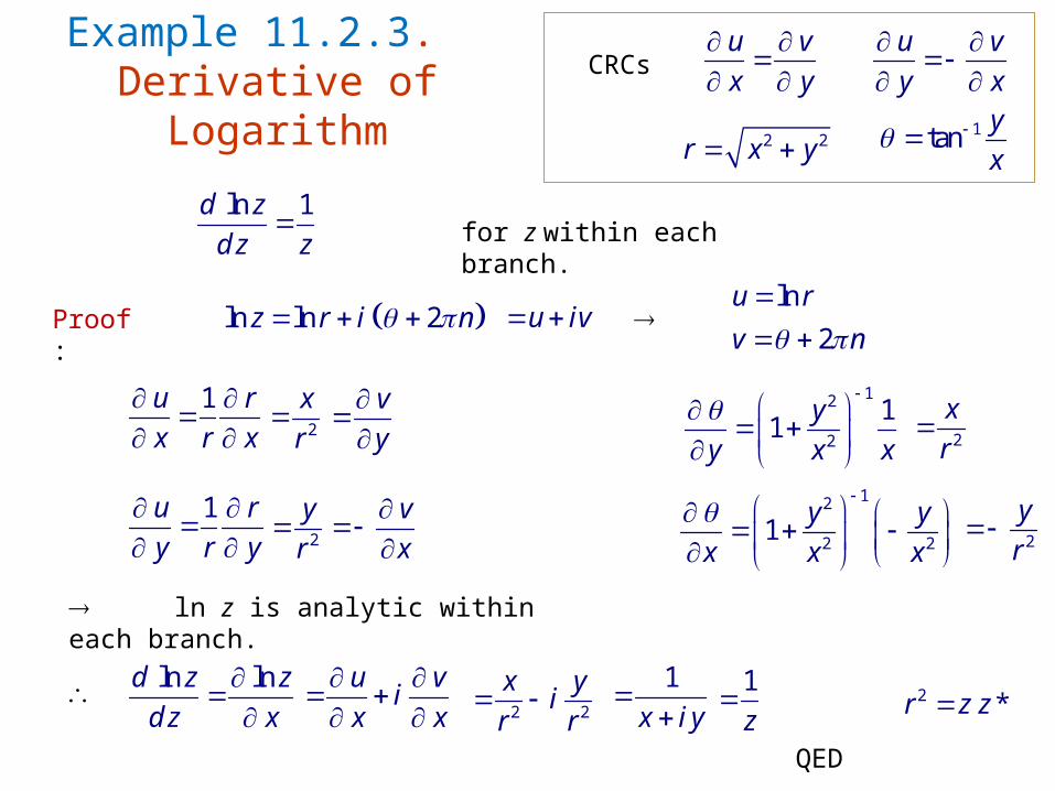
Example 11.2.3.Derivative of Logarithm
ln 1d zd z z
Proof : ln ln 2z r i n
for z within each branch.
u iv ln
2u rv n
u vx y
u vy x
CRCs
1u rx r x
2
xr
2 2r x y 1tan y
x
vy
12
2
11 yy x x
2
xr
1u ry r y
2
yr
vx
12
2 21 y yx x x
2
yr
ln z is analytic within each branch.
ln lnd z zd z x
u vix x
2 2
x yir r
1
x i y
1z
2 *r z z
QED
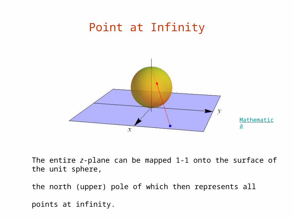
Point at Infinity
The entire z-plane can be mapped 1-1 onto the surface of the unit sphere,
the north (upper) pole of which then represents all points at infinity.
Mathematica
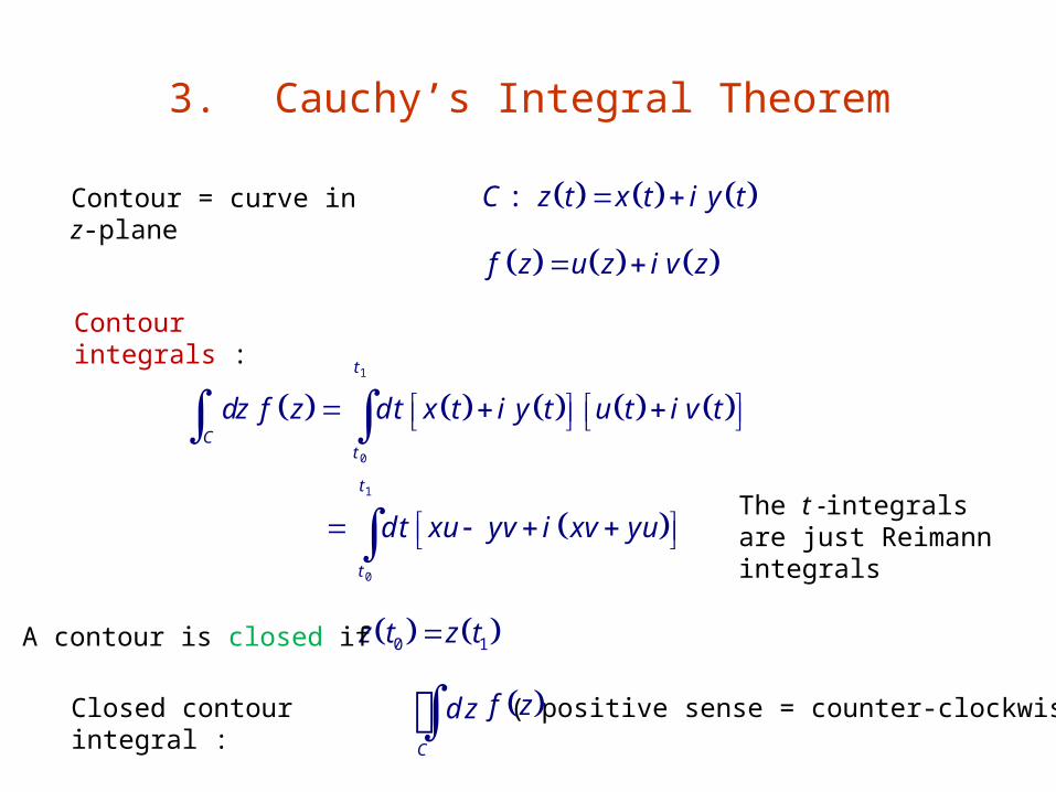
3. Cauchy’s Integral Theorem
Contour integrals :
:C z t x t i y t Contour = curve in z-plane
1
0
t
Ct
dz f z d t x t i y t u t i v t
f z u z i v z
1
0
t
t
d t xu yv i xv yu The t -integrals are just Reimann integrals
Closed contour integral :
0 1z t z tA contour is closed if
( positive sense = counter-clockwise ) C
f zd z
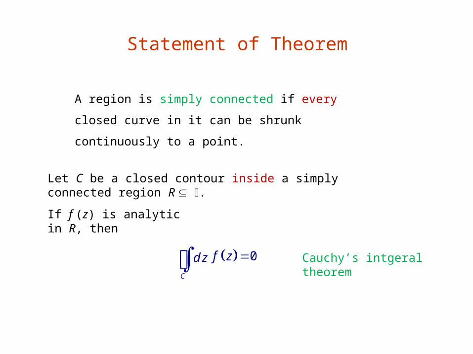
Statement of Theorem
Let C be a closed contour inside a simply connected region R .
If f (z) is analytic in R, then
0C
f zd z
A region is simply connected if every closed curve in it
can be shrunk continuously to a point.
Cauchy’s intgeral theorem
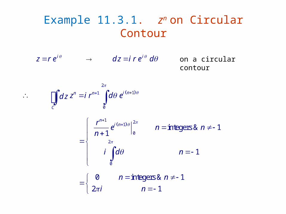
Example 11.3.1. zn on Circular Contour
2
11
0
i nn n
C
z i r d ed z
iz r e id z i r e d on a circular contour
1 21
0
2
0
integers & 11
1
ni nr e n n
n
i d n
0 integers & 1
2 1n n
i n
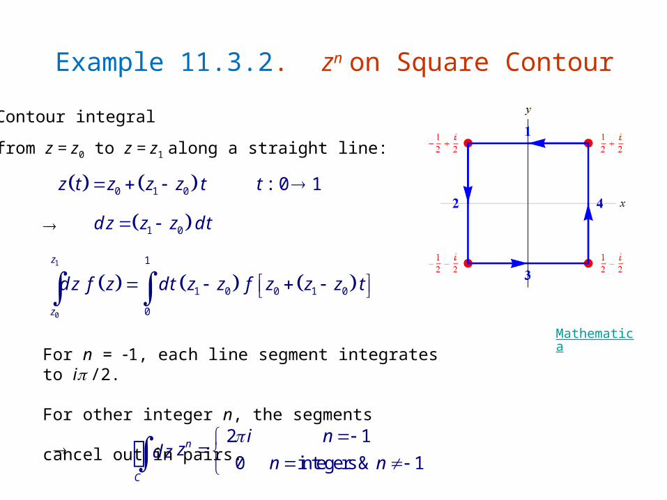
Example 11.3.2. zn on Square Contour
Contour integral
from z = z0 to z = z1 along a straight line:
0 1 0 : 0 1z t z z z t t
1 0d z z z d t
1
0
1
1 0 0 1 0
0
z
z
d z f z d t z z f z z z t
2 10 integers & 1
n
C
i nzd z n n
Mathematica
For n = 1, each line segment integrates to i /2.
For other integer n, the segments cancel out in pairs.
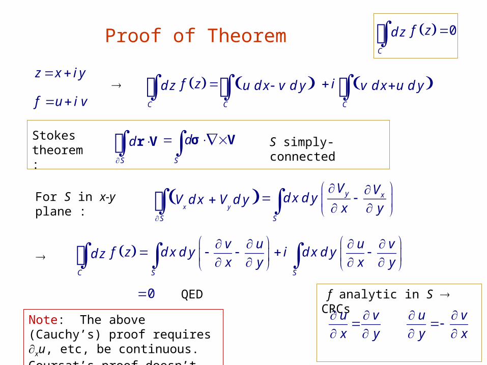
f analytic in S CRCs
Proof of Theorem 0C
f zd z z x i y
f u i v
C C C
f z id z u d x v d y v d x u d y Stokes theorem :
S S
dd
σ Vr V
For S in x-y plane : x y
y x
S S
V Vd x d yV d x V d yx y
C S S
v u u vf z d x d y i d x d yd zx y x y
0
S simply-connected
QED
u vx y
u vy x
Note: The above (Cauchy’s) proof requires xu, etc, be continuous. Goursat’s proof doesn’t.
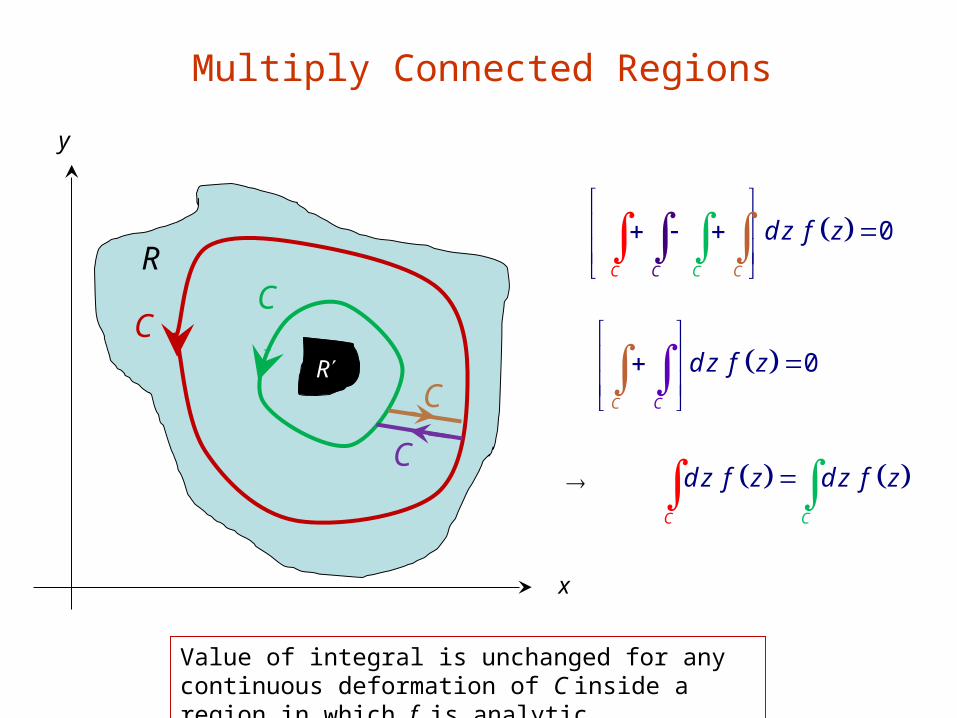
Multiply Connected Regions
y
x
R
R
CC
0CC C C
d z f z
C
C
0C C
d z f z
C C
d z f z d z f z
Value of integral is unchanged for any continuous deformation of C inside a region in which f is analytic.
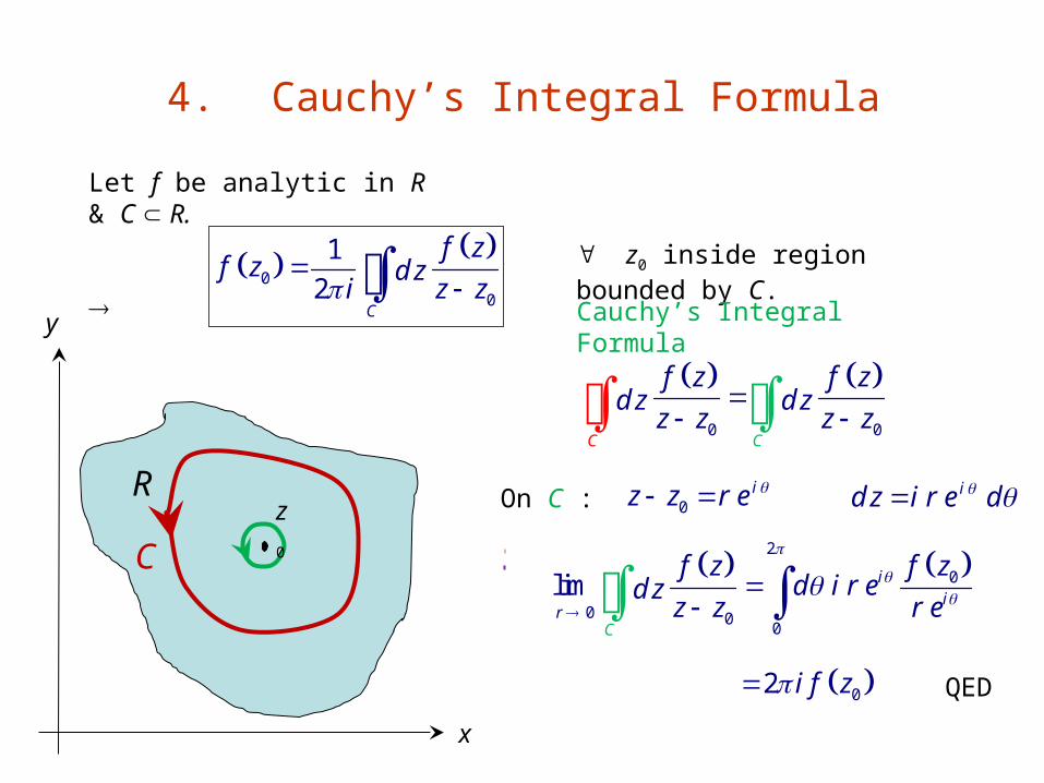
4. Cauchy’s Integral Formula
Let f be analytic in R & C R.
0
0
12
C
f zf z d z
i z z
z0 inside region bounded by C.
Cauchy’s Integral Formula
R
C
y
x
z0
0 0
CC
f z f zd z d z
z z z z
2
0
0 0 0
limC
ii
r
f z f zd i r ed z
z z r e
On C : 0iz z r e id z i r e d
02 i f z QED
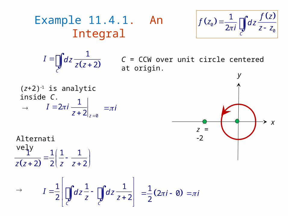
Example 11.4.1. An Integral
1
2C
I d zz z
C = CCW over unit circle centered at origin.
1 1 1 1
2 2 2z z z z
i0
122 z
I iz
Alternatively
0
0
12
C
f zf z d z
i z z
(z+2)1 is analytic inside C.
1 1 12 2
C C
I d z d zz z
1 2 0
2i i
y
x
z = 2
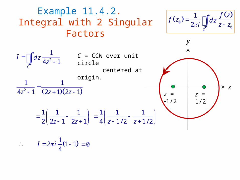
Example 11.4.2.Integral with 2 Singular Factors
2
14 1
C
I d zz
C = CCW over unit circle
centered at origin.
2
1 14 1 2 1 2 1z z z
1 1 12 2 1 2 1z z
1 1 14 1 / 2 1 / 2z z
12 1 14
I i 0
0
0
12
C
f zf z d z
i z z
y
xz = 1/2 z = 1/2
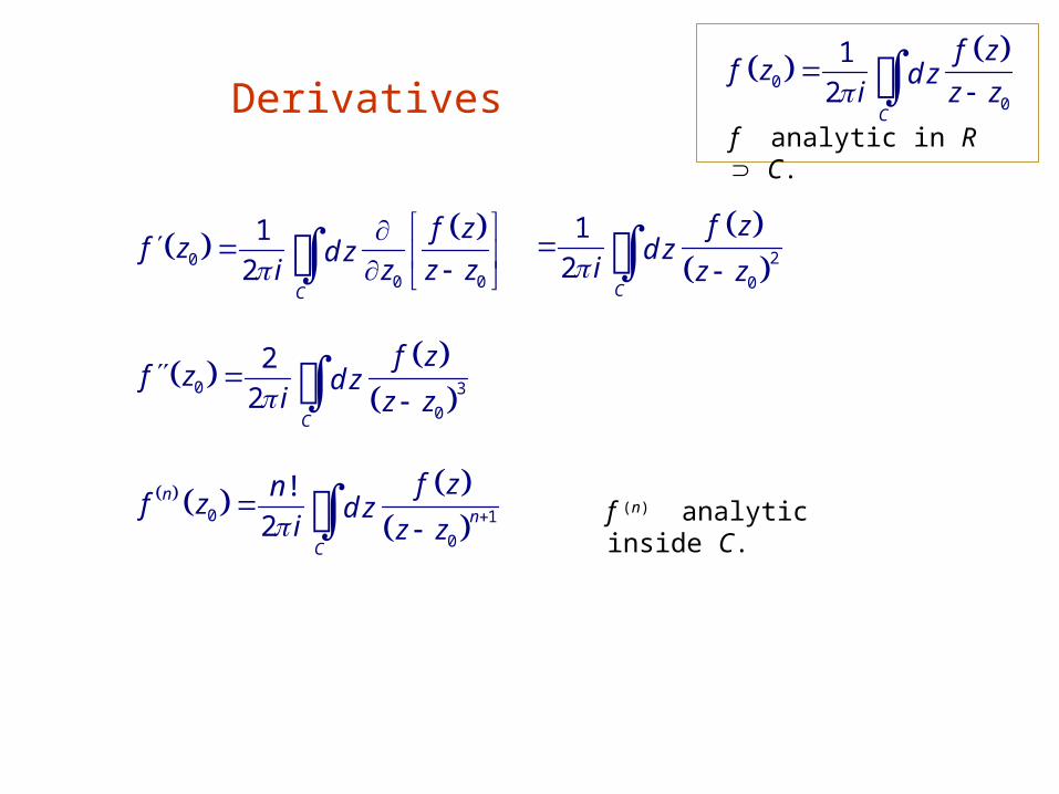
Derivatives
00
12
C
f zf z d z
i z z
0
0 0
12
C
f zf z d z
i z z z
2
0
12
C
f zd z
i z z
0 1
0
!2
nn
C
f znf z d zi z z
0 3
0
22
C
f zf z d z
i z z
f analytic in R C.
f (n) analytic inside C.
Let
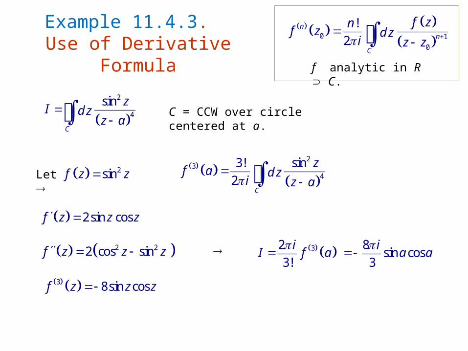
Example 11.4.3.Use of Derivative Formula
2
4sin
C
zI d zz a
C = CCW over circle centered at a.
0 1
0
!2
nn
C
f znf z d zi z z
f analytic in R C.
23
43! sin
2C
zf a d zi z a
2sinf z z
2sin cosf z z z
2 22 cos sinf z z z
3 8sin cosf z z z
323!
iI f a
8 sin cos3
i a a
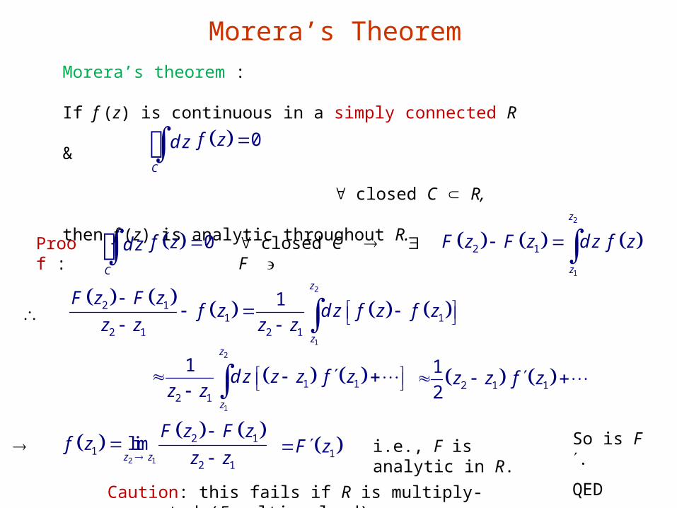
Morera’s TheoremMorera’s theorem :
If f (z) is continuous in a simply connected R &
closed C R,
then f (z) is analytic throughout R.
0C
f zd z
0C
f zd z Proof : closed C F 2
1
2 1
z
z
F z F z d z f z
2
1
2 11 1
2 1 2 1
1z
z
F z F zf z d z f z f z
z z z z
2
1
1 12 1
1z
z
d z z z f zz z
2 1 112
z z f z
2 1
2 11
2 1
limz z
F z F zf z
z z
1F z i.e., F is analytic in R. So is F .
QEDCaution: this fails if R is multiply-connected (F multi-valued).
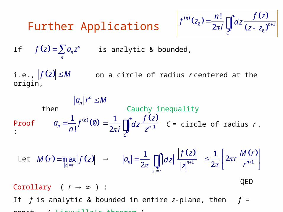
If is analytic & bounded,
i.e., on a circle of radius r centered at the origin,
then Cauchy inequality
Further Applications
nn
n
f z a z
f z M
nna r M
Proof : 1 0!
nna f
n
1
12 n
C
f zd z
i z
0 1
0
!2
nn
C
f znf z d zi z z
1
1 22 n
M rr
r
Let max
z rM r f z
1
12n n
z r
f za d z
z
QED
C = circle of radius r .
Corollary ( r ) :
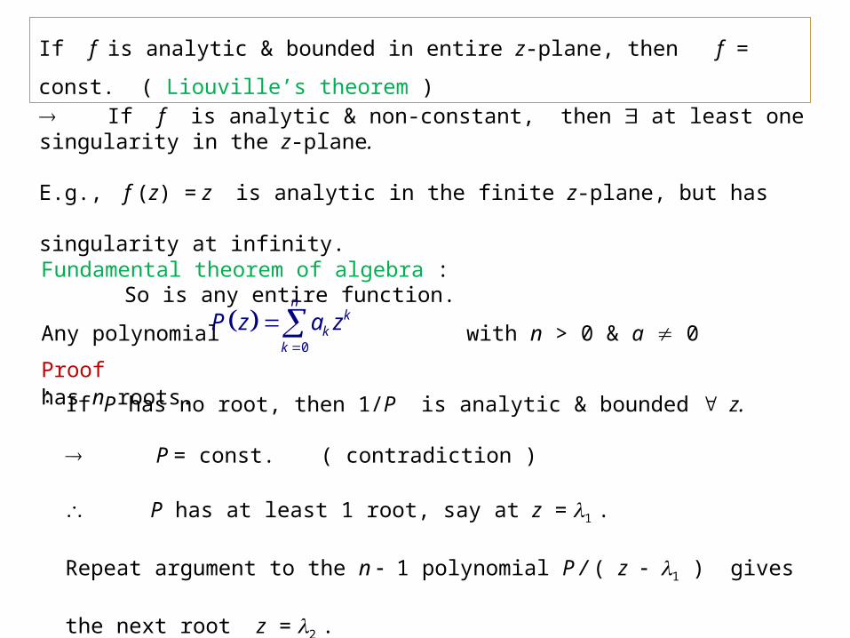
If f is analytic & bounded in entire z-plane, then f = const. ( Liouville’s theorem )
If f is analytic & bounded in entire z-plane, then f = const. ( Liouville’s theorem )
If f is analytic & non-constant, then at least one singularity in the z-plane.
E.g., f (z) = z is analytic in the finite z-plane, but has singularity at infinity.
So is any entire function.
Fundamental theorem of algebra :
Any polynomial with n > 0 & a 0 has n roots. 0
nk
kk
P z a z
Proof :
If P has no root, then 1/P is analytic & bounded z.
P = const. ( contradiction )
P has at least 1 root, say at z = 1 .
Repeat argument to the n 1 polynomial P / ( z 1 ) gives the next root z = 2 .
This can be repeated until P is reduced to a const, thus giving n roots.
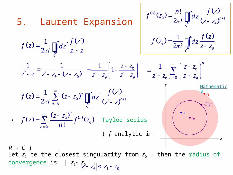
Taylor series
( f analytic in R C )
5. Laurent Expansion
0
0
12
C
f zf z d z
i z z
12
C
f zf z d z
i z z
0 0
1 1z z z z z z
1
0
0 0
1 1 z zz z z z
0
00 0
1n
n
z zz z z z
0 1
0
12
nn
nC
f zf z z z d z
i z z
0 1
0
!2
nn
C
f znf z d zi z z
00
0 !
nn
n
z zf z f z
n
Let z1 be the closest singularity from z0 , then the radius of convergence is | z1 z0 |.
i.e., series converges for 0 1 0z z z z
Mathematica

Laurent Series
Mathematica
Let f be analytic within an annular region
0r z z R
0
0
12
C
f zf z d z
i z z
0 1
0
!2
nn
C
f znf z d zi z z
21
12
CC
f zf z d z
i z z
21
0 01 10 00 0
1 1 12 2
C
n nn n
n nC
f zf z z z z z f zd z d z
i iz z z z
0
00 0 0 0
1 1 1n
n
z zz z z z z z z z z z
C1 :
0
00 0
1 1n
n
z zz z z z z z
C2 :
21
0 01 10 00 0
1 1 12 2
C
n nn n
n nC
f zf z z z z z f zd z d z
i iz z z z
2 2
1
0 01 10 0 0
1
C C
n nn n
n n
f zz z f z z zd z d z
z z z z
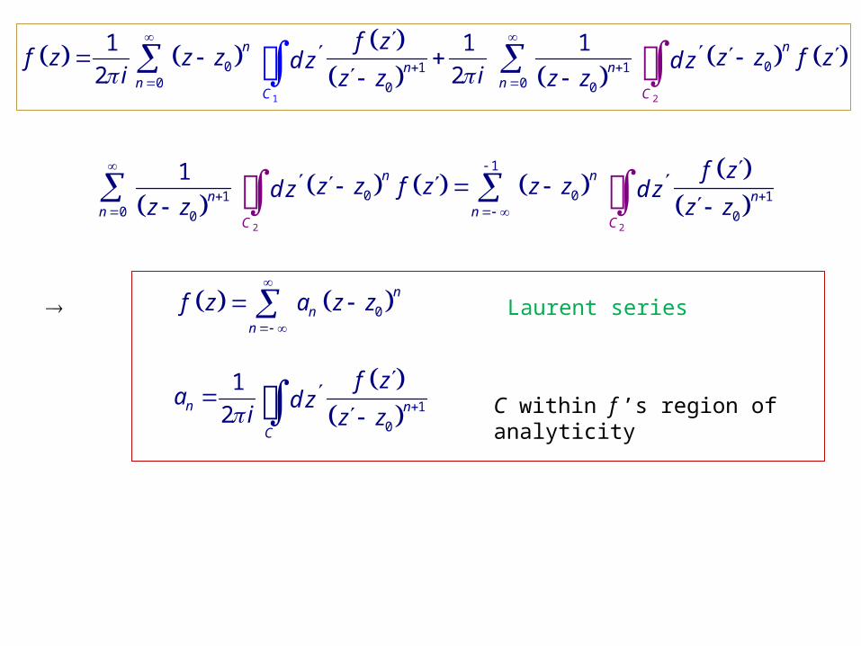
0n
nn
f z a z z
Laurent series
1
0
12n n
C
f za d z
i z z
C within f ’s region of analyticity
Consider expansion about f is analytic for
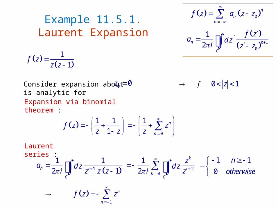
Example 11.5.1.Laurent Expansion
0n
nn
f z a z z
1
0
12n n
C
f za d z
i z z
1
1f z
z z
0 0z 0 1z
1 11
f zz z
Expansion via binomial theorem :
0
1 n
n
zz
Laurent series :
1
1 12 1n n
C
a d zi z z z
1 10
notherwise
2
0
12
k
nk
C
zd z
i z
1
n
n
f z z
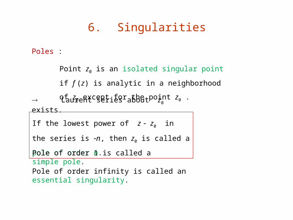
6. Singularities
Poles :
Point z0 is an isolated singular point if f (z) is analytic
in a neighborhood of z0 except for the point z0 .
Laurent series about z0 exists.
If the lowest power of z z0 in the series is n,
then z0 is called a pole of order n.
Pole of order 1 is called a simple pole.
Pole of order infinity is called an essential singularity.
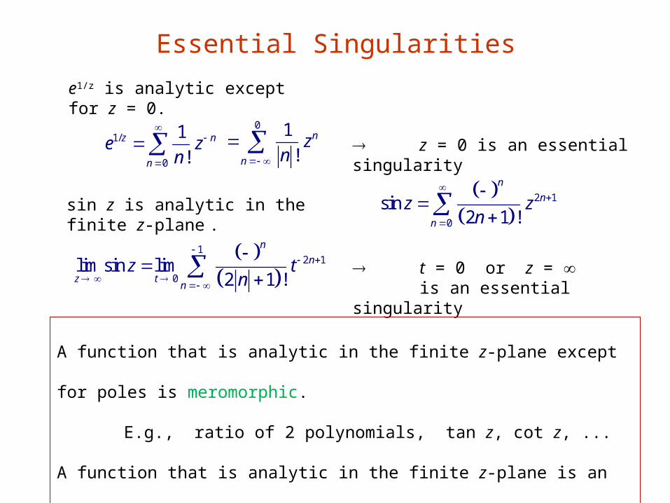
Essential Singularities
1/
0
1!
z n
n
e zn
0 1
!n
n
zn
z = 0 is an essential singularity
e1/z is analytic except for z = 0.
sin z is analytic in the finite z-plane .
2 1
0
sin2 1 !
nn
n
z zn
12 1
0lim sin lim
2 1 !
nn
z tn
z tn
t = 0 or z = is an essential singularity
A function that is analytic in the finite z-plane except for poles is meromorphic.
E.g., ratio of 2 polynomials, tan z, cot z, ...
A function that is analytic in the finite z-plane is an entire function.
E.g., ez , sin z, cos z, ...
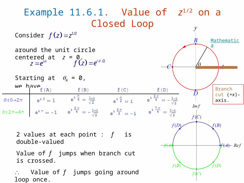
Starting at A = 0, we have
Consider
around the unit circle centered at z = 0.
Example 11.6.1. Value of z1/2 on a Closed Loop
1/2f z z
2 values at each point : f is double-valued
/2if z e
Mathematica
Branch cut (+x)-axis.
iz e
Value of f jumps when branch cut is crossed.
Value of f jumps going around loop once.
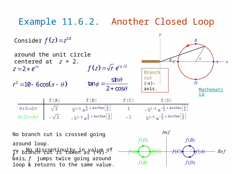
Example 11.6.2. Another Closed Loop
Mathematica
Branch cut (x)-axis.
Consider
around the unit circle centered at z = 2.
2 iz e
1/2f z z
/ 2if z r e
2 10 6cosr sintan
2 cos
No branch cut is crossed going around loop. No discontinuity in value of f .
If branch cut is taken as (+x)-axis, f jumps twice going around loop & returns to the same value.
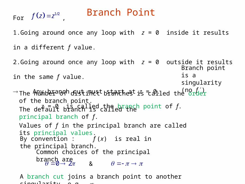
Branch PointFor ,
1.Going around once any loop with z = 0 inside it results in a different f value.
2.Going around once any loop with z = 0 outside it results in the same f value.
Any branch cut must start at z = 0.
z = 0 is called the branch point of f.
1/2f z z
The number of distinct branches is called the order of the branch point.
The default branch is called the principal branch of f.
Values of f in the principal branch are called its principal values.
Common choices of the principal branch are
0 2 &
Branch point is a singularity (no f )
By convention : f (x) is real in the principal branch.
A branch cut joins a branch point to another singularity, e.g., .

Example 11.6.3.ln z has an Infinite Number of Branches
iz r e 2i nr e n = 0, 1, 2, ...
ln ln 2z r i n Infinite number of branches
z = 0 is the branch point (of order ).ln 1d zd z z
Similarly for the inverse trigonometric functions.
exp lnpz p z exp ln exp 2p r i i pn
p = integers z p is single-valued. exp 2 1i pn
p = rational = k / m z p is m-valued.
p = irrational z p is -valued.
Let
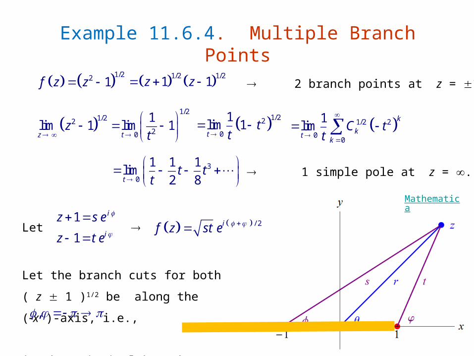
Example 11.6.4. Multiple Branch Points
1/22 1f z z 1/2 1/21 1z z 2 branch points at z = 1.
1/2
1/2220
1lim 1 lim 1z t
zt
1/22
0
1lim 1t
tt
1/2 2
00
1limk
ktk
C tt
3
0
1 1 1lim2 8t
t tt
1 simple pole at z = .
1
1
i
i
z s e
z t e
/ 2if z st e
Let the branch cuts for both ( z 1 )1/2
be along the (x )-axis, i.e.,
in the principal branch.
,
Mathematica
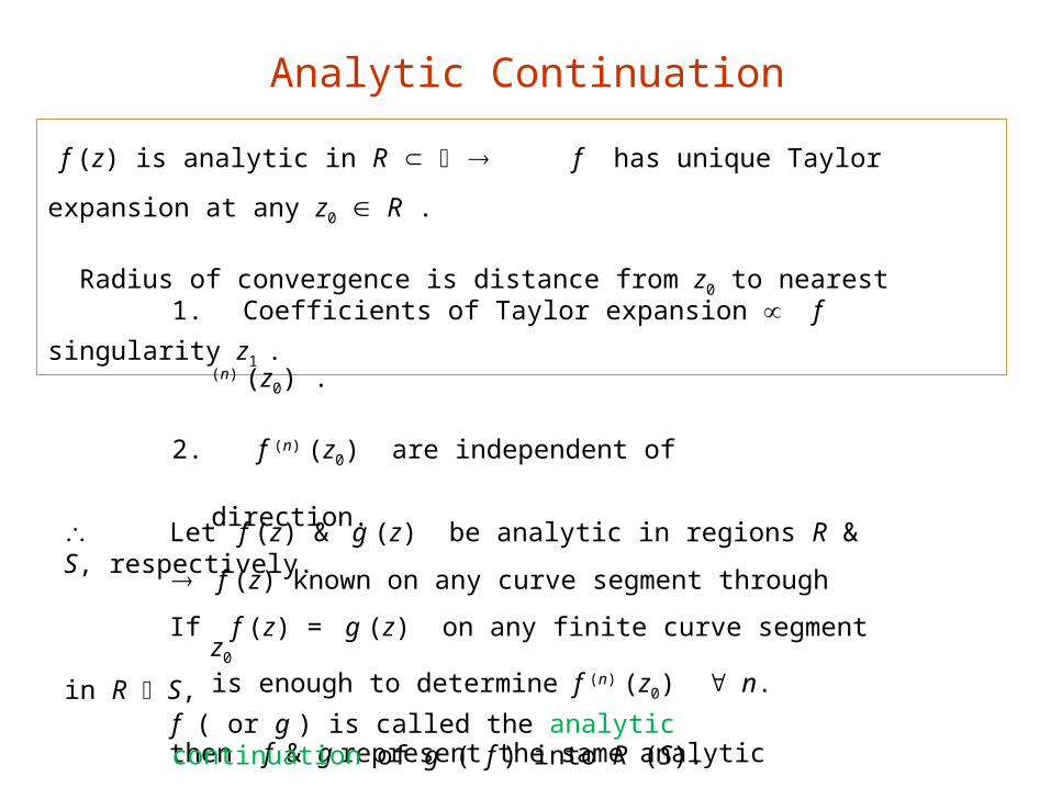
Analytic Continuation
f (z) is analytic in R f has unique Taylor expansion at any z0 R .
Radius of convergence is distance from z0 to nearest singularity z1 .
1. Coefficients of Taylor expansion f (n) (z0) .
2. f (n) (z0) are independent of direction.
f (z) known on any curve segment through z0
is enough to determine f (n) (z0) n. Let f (z) & g (z) be analytic in regions R & S, respectively.
If f (z) = g (z) on any finite curve segment in R S,
then f & g represent the same analytic function in R S.
f ( or g ) is called the analytic continuation of g ( f ) into R (S).
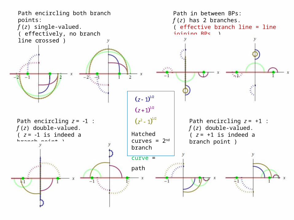
Path encircling both branch points:f (z) single-valued.( effectively, no branch line crossed )
Path in between BPs:f (z) has 2 branches.( effective branch line = line joining BPs. )
Path encircling z = 1 :f (z) double-valued.( z = 1 is indeed a branch point )
Path encircling z = +1 :f (z) double-valued.( z = +1 is indeed a branch point )Hatched curves
= 2nd branch
curve = path
1/
1/2
1 2
2
2
/
1
1
1z
z
z
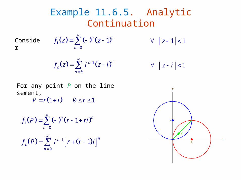
Example 11.6.5. Analytic Continuation
Consider 10
1n n
n
f z z
12
0
nn
n
f z i z i
1 1z
1z i
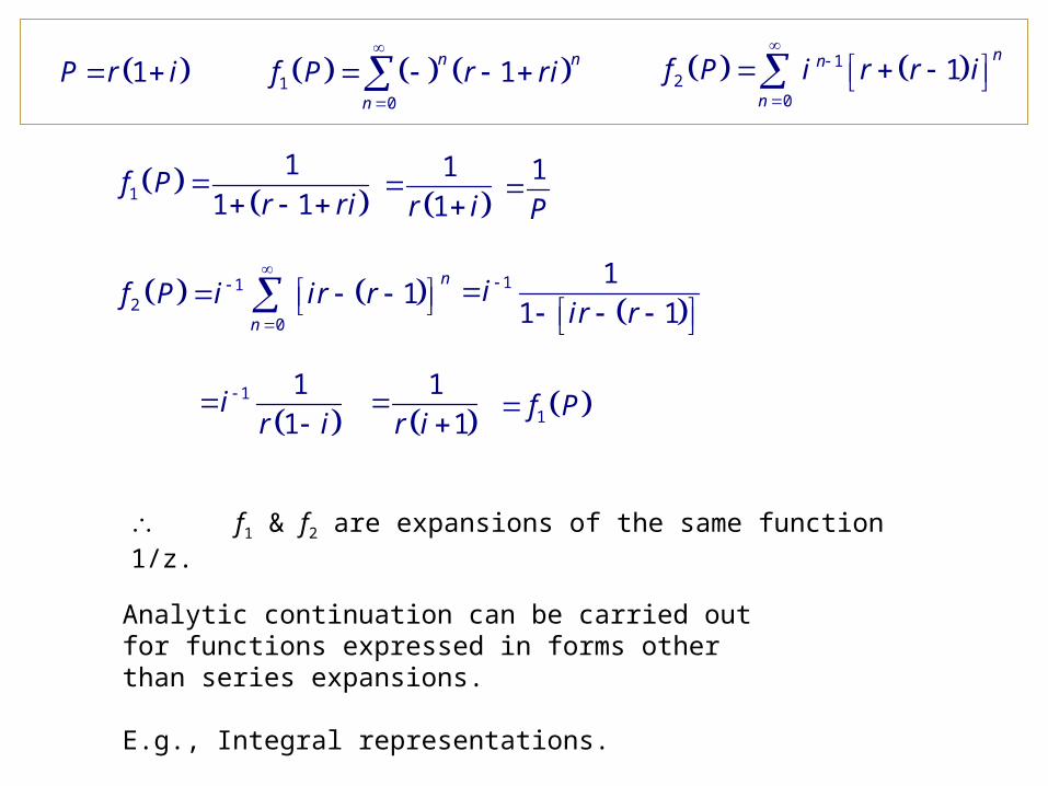
For any point P on the line sement,
1 0 1P r i r
10
1n n
n
f P r ri
12
0
1nn
n
f P i r r i
10
1n n
n
f P r ri
12
0
1nn
n
f P i r r i
11
1 1f P
r ri
12
0
1n
n
f P i ir r
1
1r i
1 1
1 1i
ir r
1 1
1i
r i
1
1r i
1f P
f1 & f2 are expansions of the same function 1/z.
1P
1P r i
Analytic continuation can be carried out for functions expressed in forms other than series expansions.
E.g., Integral representations.


