
Complex VariablesLaplace Transform – Z Transform
Prof. Nicolas Dobigeon
University of ToulouseIRIT/INP-ENSEEIHT
http://www.enseeiht.fr/[email protected]
Prof. Nicolas Dobigeon Complex variables - LT & ZT 1 / 105

Framework
Organization
I 7 course & exercice sessions (1h45),
I 1 written exam (shared with Vector Analysis)
Bibliography
I Handout ENSEEIHT
I Books
I S. D. Chatterji, Cours d’analyse (vol. 2), Presses Polytechniques etUniversitaires Romandes, 1997
I Spiegel, Variables complexes (cours et problemes), Serie Schaum,McGraw Hill., 1973
Prof. Nicolas Dobigeon Complex variables - LT & ZT 2 / 105
Motivation
Applications
I Analysis and numerical calculus,
I Laplace transformCircuit theory,
I Z transformSampled systems,Digital filtering,Digital signal processing,
Prerequisites
I Usual algebra of complex numbers: properties, geometry associated withthe vector representation,
I Differentiable functions of two real variables,
I curvilinear integrals
Prof. Nicolas Dobigeon Complex variables - LT & ZT 3 / 105

Outline
Some Generalities
Usual functions
Holomorphic functions
Integration and Cauchy theorem
Residue theorem
Laplace transform
Z transform
Prof. Nicolas Dobigeon Complex variables - LT & ZT 4 / 105

Some Generalities
Outline
Some GeneralitiesIntroductionLimits - continuity
Usual functions
Holomorphic functions
Integration and Cauchy theorem
Residue theorem
Laplace transform
Z transform
Prof. Nicolas Dobigeon Complex variables - LT & ZT 5 / 105

Some Generalities
Introduction
Outline
Some GeneralitiesIntroductionLimits - continuity
Usual functions
Holomorphic functions
Integration and Cauchy theorem
Residue theorem
Laplace transform
Z transform
Prof. Nicolas Dobigeon Complex variables - LT & ZT 6 / 105
Some Generalities
Introduction
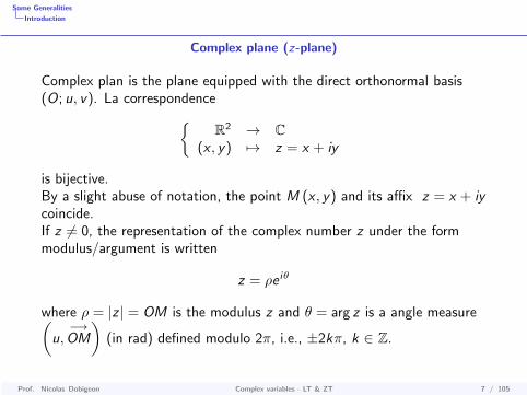
Complex plane (z-plane)
Complex plan is the plane equipped with the direct orthonormal basis(O; u, v). La correspondence
R2 → C(x , y) 7→ z = x + iy
is bijective.By a slight abuse of notation, the point M (x , y) and its affix z = x + iycoincide.If z 6= 0, the representation of the complex number z under the formmodulus/argument is written
z = ρe iθ
where ρ = |z | = OM is the modulus z and θ = arg z is a angle measure(u,−→OM
)(in rad) defined modulo 2π, i.e., ±2kπ, k ∈ Z.
Prof. Nicolas Dobigeon Complex variables - LT & ZT 7 / 105

Some Generalities
Introduction
Complex function of the z-variable
For any function f of complex variable
f :
C → C
z = x + iy 7→ f (z) = P(x , y) + iQ(x , y)
we can define a function F :
F :
R2 → R2
(x , y) 7→ F (x , y) = (P(x , y),Q(x , y))
Prof. Nicolas Dobigeon Complex variables - LT & ZT 8 / 105
Some Generalities
Limits - continuity
Outline
Some GeneralitiesIntroductionLimits - continuity
Usual functions
Holomorphic functions
Integration and Cauchy theorem
Residue theorem
Laplace transform
Z transform
Prof. Nicolas Dobigeon Complex variables - LT & ZT 9 / 105

Some Generalities
Limits - continuity
Limits - continuity
C is a vector space on R equipped with the norm ‖z‖ = |z |.Let f define a complex variable function and z0 = x0 + iy0 and l twocomplex numbers.
Definition: limit
limz−→z0
f (z) = l or f (z) −→z−→z0
l
means:∀ε > 0, ∃η > 0, |z − z0| < η =⇒ |f (z)− l | < ε
Definition: continuity
f continue at z0 ⇐⇒ limz−→z0
f (z) = f (z0)
⇐⇒ P(x , y) and Q(x , y) continue at (x0, y0)
Prof. Nicolas Dobigeon Complex variables - LT & ZT 10 / 105

Some Generalities
Limits - continuity
Limits - continuity
Without any demonstration, we will admit that the standard operationson the limits or continuous functions are the same as those obtained forfunctions from R2 → R or from R→ R
Warning !If P(x , y) is continuous at the point (x0, y0), then
x 7→ P(x , y0) is continuous at x = x0
y 7→ P(x0, y) is continuous at y = y0
The reciprocal is wrong!
Prof. Nicolas Dobigeon Complex variables - LT & ZT 11 / 105
Some Generalities
Limits - continuity
Complex infinity
The complex infinity denoted ∞ is the unique complex number ensuringthe following properties with a ∈ C:
∞×∞ = ∞, |∞| =∞∞/a = ∞, a/∞ = 0, a×∞ =∞
I Representation on the Poincare sphere,
I Extensions of the limit and neighboring definitions around infinity.
Prof. Nicolas Dobigeon Complex variables - LT & ZT 12 / 105
Usual functions
Outline
Some Generalities
Usual functionsAlgebraic functionsFunctions defined by power seriesMultivalued functions (or multifunctions)
Holomorphic functions
Integration and Cauchy theorem
Residue theorem
Laplace transform
Z transform
Prof. Nicolas Dobigeon Complex variables - LT & ZT 13 / 105

Usual functions
Algebraic functions
Outline
Some Generalities
Usual functionsAlgebraic functionsFunctions defined by power seriesMultivalued functions (or multifunctions)
Holomorphic functions
Integration and Cauchy theorem
Residue theorem
Laplace transform
Z transform
Prof. Nicolas Dobigeon Complex variables - LT & ZT 14 / 105

Usual functions
Algebraic functions
Algebraic functions
Functions Definition Continuiy Associated TG
z 7−→ z + a C C Translationz 7−→ a z C C Similarityz 7−→ 1
z C∗ C∗ Inversion then symetry Ox
z 7−→ az+bcz+d C \
− d
c
C \
− d
c
...
Prof. Nicolas Dobigeon Complex variables - LT & ZT 15 / 105
Usual functions
Functions defined by power series
Outline
Some Generalities
Usual functionsAlgebraic functionsFunctions defined by power seriesMultivalued functions (or multifunctions)
Holomorphic functions
Integration and Cauchy theorem
Residue theorem
Laplace transform
Z transform
Prof. Nicolas Dobigeon Complex variables - LT & ZT 16 / 105
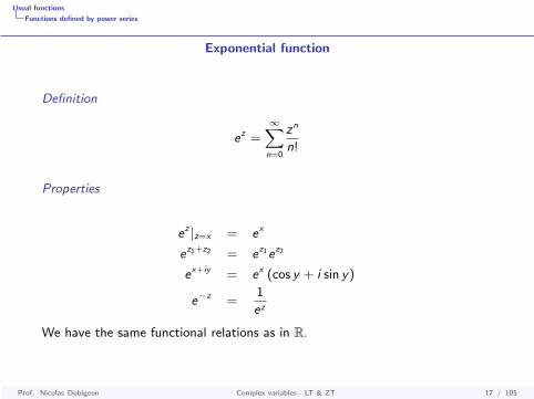
Usual functions
Functions defined by power series
Exponential function
Definition
ez =∞∑n=0
zn
n!
Properties
ez |z=x = ex
ez1+z2 = ez1ez2
ex+iy = ex (cos y + i sin y)
e−z =1
ez
We have the same functional relations as in R.
Prof. Nicolas Dobigeon Complex variables - LT & ZT 17 / 105
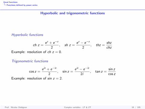
Usual functions
Functions defined by power series
Hyperbolic and trigonometric functions
Hyperbolic functions
ch z =ez + e−z
2, sh z =
ez − e−z
2, thz =
shz
chzExample: resolution of ch z = 0.
Trigonometric functions
cos z =e iz + e−iz
2, sin z =
e iz − e−iz
2i, tan z =
sin z
cos zExample: resolution of sin z = 2.
Prof. Nicolas Dobigeon Complex variables - LT & ZT 18 / 105

Usual functions
Functions defined by power series
Hyperbolic and trigonometric functions
PropertiesFunctions Definition set Continuity set
exp C Cch C Csh C Cth C\
i(π2
+ kπ), k ∈ Z
C\i(π2
+ kπ), k ∈ Z
cos C Csin C Ctan C\
π2
+ kπ, k ∈ Z
C\π2
+ kπ, k ∈ Z
Changing rulescos iz = ch zsin iz = i sh z
tan iz = i th zand
ch iz = cos zsh iz = i sin zth iz = i tan z
Prof. Nicolas Dobigeon Complex variables - LT & ZT 19 / 105
Usual functions
Multivalued functions (or multifunctions)
Outline
Some Generalities
Usual functionsAlgebraic functionsFunctions defined by power seriesMultivalued functions (or multifunctions)
Holomorphic functions
Integration and Cauchy theorem
Residue theorem
Laplace transform
Z transform
Prof. Nicolas Dobigeon Complex variables - LT & ZT 20 / 105
Usual functions
Multivalued functions (or multifunctions)
Multivalued function
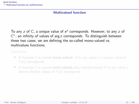
To any z of C, a unique value of ez corresponds. However, to any z ofC∗, an infinity of values of arg z corresponds. To distinguish betweenthese two cases, we are defining the so-called mono-valued vs.multivalues functions.
Definitions
I A function f is named mono-valued if to any value z a unique value off (z) corresponds.
I A function f is named multi-valued (aka multifunctions) if to any value zseveral distinct values of f (z) correspond.
Prof. Nicolas Dobigeon Complex variables - LT & ZT 21 / 105
Usual functions
Multivalued functions (or multifunctions)
Multivalued function
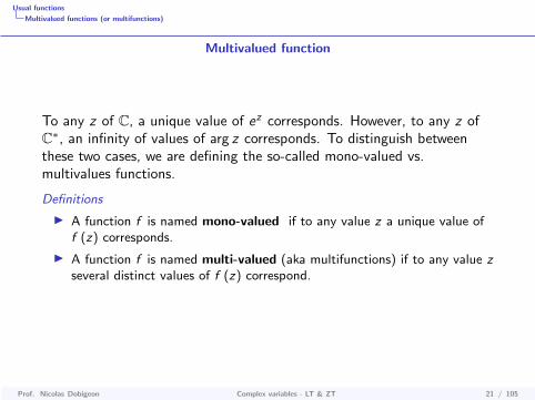
To any z of C, a unique value of ez corresponds. However, to any z ofC∗, an infinity of values of arg z corresponds. To distinguish betweenthese two cases, we are defining the so-called mono-valued vs.multivalues functions.
Definitions
I A function f is named mono-valued if to any value z a unique value off (z) corresponds.
I A function f is named multi-valued (aka multifunctions) if to any value zseveral distinct values of f (z) correspond.
Prof. Nicolas Dobigeon Complex variables - LT & ZT 21 / 105

Usual functions
Multivalued functions (or multifunctions)
Multivalued functions
Examples
I The argument function :
C∗ −→ Rz 7−→ arg z
is a multi-valued function.
I The functions introduce earlier are mono-valued.
Study of the multivalued functionsTo study the multivalued functions, we make them mono-valued by defining itsrestrictions (or “branches”) of rank k.
Prof. Nicolas Dobigeon Complex variables - LT & ZT 22 / 105
Usual functions
Multivalued functions (or multifunctions)
Argument function
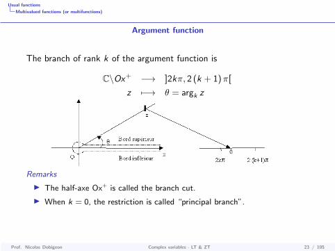
The branch of rank k of the argument function is
C\Ox+ −→ ]2kπ, 2 (k + 1)π[
z 7−→ θ = argk z
Remarks
I The half-axe Ox+ is called the branch cut.
I When k = 0, the restriction is called “principal branch”.
Prof. Nicolas Dobigeon Complex variables - LT & ZT 23 / 105

Usual functions
Multivalued functions (or multifunctions)
Argument function: other definition (more general)
The branch of rank k of the argument function is
C\Dα −→ ]α + 2kπ, α + 2 (k + 1)π[
z 7−→ θ = argk,α z
Remarks
I With this definition, the half-line (or ray) Dα with origin O and angle α isthe branch cut.
Prof. Nicolas Dobigeon Complex variables - LT & ZT 24 / 105

Usual functions
Multivalued functions (or multifunctions)
Multifunctions
Definitions
I Continuity values: values on the upper and lower sides of the branch cut.
I The point O at the origin of the branch cut is called the branch point.
Remarks
I How to represent the branch cut?
I Closed paths enclosing the branch point → branch change [WARNING]
I Closed paths enclosing the branch point → no branch change
Prof. Nicolas Dobigeon Complex variables - LT & ZT 25 / 105
Usual functions
Multivalued functions (or multifunctions)
Power functions
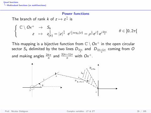
The branch of rank k of z 7→ z1n is
C \ Ox+ → Sk
z 7→ z1n
(k) = |z |1n e i
1n argk (z) = ρ
1n e i
θn e i
2kπn
θ ∈ ]0, 2π[
This mapping is a bijective function from C \ Ox+ in the open circularsector Sk delimited by the two lines D 2kπ
nand D 2(k+1)π
ncoming from O
and making angles 2kπn and 2(k+1)π
n with Ox+.
Prof. Nicolas Dobigeon Complex variables - LT & ZT 26 / 105
Usual functions
Multivalued functions (or multifunctions)
Power functions
Extensions
I Function z 7→ (z − a)1n .
I Function z 7→ (z − a)α, α ∈ R.
Example
Restriction of z 7→ (z + 1)12 .
Prof. Nicolas Dobigeon Complex variables - LT & ZT 27 / 105

Usual functions
Multivalued functions (or multifunctions)
Logarithm function
The restriction of rank k of z 7→ log(z) is C \ Ox+ → Bk
z = |z |e iθ+i2kπ 7→ logk(z) = ln |z |+ argk(z)= ln ρ+ iθ + i2kπ
where Bk is the open strip-like set defined by:z / Imz ∈ ]2kπ, 2(k + 1)π[ .
Extension
I Function z 7→ zα, α ∈ C defined by zαk = eα logk (z).
Prof. Nicolas Dobigeon Complex variables - LT & ZT 28 / 105
Holomorphic functions
Outline
Some Generalities
Usual functions
Holomorphic functionsDifferentiable functions of two variables (reminders...)Derivative of a complex variable functionHolomorphic functionsComplement : harmonic functions
Integration and Cauchy theorem
Residue theorem
Laplace transform
Z transform
Prof. Nicolas Dobigeon Complex variables - LT & ZT 29 / 105

Holomorphic functions
Differentiable functions of two variables (reminders...)
Outline
Some Generalities
Usual functions
Holomorphic functionsDifferentiable functions of two variables (reminders...)Derivative of a complex variable functionHolomorphic functionsComplement : harmonic functions
Integration and Cauchy theorem
Residue theorem
Laplace transform
Z transform
Prof. Nicolas Dobigeon Complex variables - LT & ZT 30 / 105
Holomorphic functions
Differentiable functions of two variables (reminders...)
Differentiable functions of two variables
A function P (x , y) is differentiable at the point (x0, y0) when it isdefined in an open set containing this point and:
∆P = A (x0, y0) h + B (x0, y0) k + ‖(h, k)‖ ε (h, k)
with∆P = P (x0 + h, y0 + k)− P (x0, y0)
etlim
‖(h,k)‖→0ε (h, k) = 0
Prof. Nicolas Dobigeon Complex variables - LT & ZT 31 / 105

Holomorphic functions
Derivative of a complex variable function
Outline
Some Generalities
Usual functions
Holomorphic functionsDifferentiable functions of two variables (reminders...)Derivative of a complex variable functionHolomorphic functionsComplement : harmonic functions
Integration and Cauchy theorem
Residue theorem
Laplace transform
Z transform
Prof. Nicolas Dobigeon Complex variables - LT & ZT 32 / 105

Holomorphic functions
Derivative of a complex variable function
Definition of the differentiability
Definitionf (z) differentiable at z0 if and only if
limz→z0
f (z)− f (z0)
z − z0
exists. It is denoted
f ′ (z0) = limz→z0
f (z)− f (z0)
z − z0
Example 1f (z) = z
limz→z0
z − z0
z − z0= 1, hence f est derivable en z0.
Example 2f (z) = z2
limz→z0
z2 − z20
z − z0= lim
z→z0
(z + z0) = 2z0, hence f est derivable en z0.
Prof. Nicolas Dobigeon Complex variables - LT & ZT 33 / 105

Holomorphic functions
Derivative of a complex variable function
Definition of the differentiability
Counter exampleg(z) = z
z − z0
z − z0=
(x − x0)− i (y − y0)
(x − x0) + i (y − y0)
=1− i y−y0
x−x0
1 + i y−y0x−x0
=1− im
1 + im
which depends on the slope m of the path, thus
limz→z0
z − z0
z − z0does not exist
⇒ f is not differentiable at z0.
Prof. Nicolas Dobigeon Complex variables - LT & ZT 34 / 105

Holomorphic functions
Derivative of a complex variable function
Necessary and sufficient condition
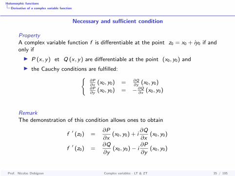
PropertyA complex variable function f is differentiable at the point z0 = x0 + iy0 if andonly if
I P (x , y) et Q (x , y) are differentiable at the point (x0, y0) and
I the Cauchy conditions are fulfilled:∂P∂x
(x0, y0) = ∂Q∂y
(x0, y0)∂P∂y
(x0, y0) = − ∂Q∂x
(x0, y0)
RemarkThe demonstration of this condition allows ones to obtain
f ′ (z0) =∂P
∂x(x0, y0) + i
∂Q
∂x(x0, y0)
f ′ (z0) =∂Q
∂y(x0, y0)− i
∂P
∂y(x0, y0)
Prof. Nicolas Dobigeon Complex variables - LT & ZT 35 / 105
Holomorphic functions
Derivative of a complex variable function
Necessary and sufficient condition
PropertyA complex variable function f is differentiable at the point z0 = x0 + iy0 if andonly if
I P (x , y) et Q (x , y) are differentiable at the point (x0, y0) and
I the Cauchy conditions are fulfilled:∂P∂x
(x0, y0) = ∂Q∂y
(x0, y0)∂P∂y
(x0, y0) = − ∂Q∂x
(x0, y0)
RemarkThe demonstration of this condition allows ones to obtain
f ′ (z0) =∂P
∂x(x0, y0) + i
∂Q
∂x(x0, y0)
f ′ (z0) =∂Q
∂y(x0, y0)− i
∂P
∂y(x0, y0)
Prof. Nicolas Dobigeon Complex variables - LT & ZT 35 / 105

Holomorphic functions
Holomorphic functions
Outline
Some Generalities
Usual functions
Holomorphic functionsDifferentiable functions of two variables (reminders...)Derivative of a complex variable functionHolomorphic functionsComplement : harmonic functions
Integration and Cauchy theorem
Residue theorem
Laplace transform
Z transform
Prof. Nicolas Dobigeon Complex variables - LT & ZT 36 / 105

Holomorphic functions
Holomorphic functions
Holomorphic functions
DefinitionA complex variable function is said holomorphic on an open set A of C if it isdifferentiable in any point of A. Notation: f ∈ H/A.
PropertiesThe properties are the same as those related to differentiable in R. Let define fand g ∈ H/A.I λf + µg ∈ H/A et (λf + µg)′ = λf ′ + µg ′
I fg ∈ H/A et (fg)′ = f ′g + fg ′
I If ∀z ∈ A, g (z) 6= 0, then:
1
g∈ H/A et
(1
g
)′= − g ′
g 2
I If f ∈ H/A, g ∈ H/f (A), then: (g f ) ∈ H/A et (g f )′ = (g ′ f ) f ′
I If f is bijective from A onto f (A), then:
f −1 ∈ H/f (A) et(f −1
)′=
1
f ′ f −1
Prof. Nicolas Dobigeon Complex variables - LT & ZT 37 / 105

Holomorphic functions
Holomorphic functions
Holomorphic functions
DefinitionA complex variable function is said holomorphic on an open set A of C if it isdifferentiable in any point of A. Notation: f ∈ H/A.
PropertiesThe properties are the same as those related to differentiable in R. Let define fand g ∈ H/A.I λf + µg ∈ H/A et (λf + µg)′ = λf ′ + µg ′
I fg ∈ H/A et (fg)′ = f ′g + fg ′
I If ∀z ∈ A, g (z) 6= 0, then:
1
g∈ H/A et
(1
g
)′= − g ′
g 2
I If f ∈ H/A, g ∈ H/f (A), then: (g f ) ∈ H/A et (g f )′ = (g ′ f ) f ′
I If f is bijective from A onto f (A), then:
f −1 ∈ H/f (A) et(f −1
)′=
1
f ′ f −1
Prof. Nicolas Dobigeon Complex variables - LT & ZT 37 / 105
Holomorphic functions
Holomorphic functions
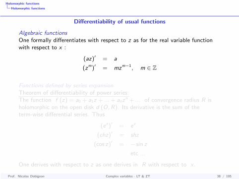
Differentiability of usual functions
Algebraic functionsOne formally differentiates with respect to z as for the real variable functionwith respect to x :
(az)′ = a
(zm)′ = mzm−1, m ∈ Z
Functions defined by series expansionTheorem of differentiability of power series:The function f (z) = a0 + a1z + ...+ anz
n + ... of convergence radius R isholomorphic on the open disk d (O,R). Its derivative is the sum of theterm-wise differential series. Thus
(ez)′ = ez
(chz)′ = shz
(cos z)′ = − sin z
etc ...
One derives with respect to z as one derives in R with respect to x .
Prof. Nicolas Dobigeon Complex variables - LT & ZT 38 / 105

Holomorphic functions
Holomorphic functions
Differentiability of multifunctions
I Derivative of logk z
Z = logk (z) = ln ρ+ iθ + 2ikπ
defined from C \ Ox+ to Bk .
One reminds that exp (logk (z)) = z . By the reciprocal formula, thederivative is given
z = f (Z) =⇒ z ′ = f ′ (Z)
Z = f −1 (z) =⇒ Z ′ =1
f ′ (f −1 (z))
Thus:
z = exp (Z) =⇒ z ′ = exp (Z)
Z = logk (z) =⇒ Z ′ =1
exp (logk (z))=
1
z
The additive constant disappears. Thus:
logk z holomorphic on C \ Ox+ et (logk)′ (z) = 1z
Prof. Nicolas Dobigeon Complex variables - LT & ZT 39 / 105

Holomorphic functions
Holomorphic functions
Differentiability of multifunctions
I Derivative of zα(k), α ∈ C
zα(k) = exp (α logk (z))
By differentiability of compound functions, one obtains:[zα(k)
]′= [α [logk (z)]]′ exp [α logk (z)]
Thus: [zα(k)
]′=α
zzα(k)
The derivative owns the same multiplicative constant. Thus
zα(k) holomorphic on C \ Ox+ et[zα(k)
]′=α
zzα(k)
Prof. Nicolas Dobigeon Complex variables - LT & ZT 40 / 105
Holomorphic functions
Complement : harmonic functions
Outline
Some Generalities
Usual functions
Holomorphic functionsDifferentiable functions of two variables (reminders...)Derivative of a complex variable functionHolomorphic functionsComplement : harmonic functions
Integration and Cauchy theorem
Residue theorem
Laplace transform
Z transform
Prof. Nicolas Dobigeon Complex variables - LT & ZT 41 / 105

Holomorphic functions
Complement : harmonic functions
Complement : harmonic functions
If we had time...
Prof. Nicolas Dobigeon Complex variables - LT & ZT 42 / 105

Integration and Cauchy theorem
Outline
Some Generalities
Usual functions
Holomorphic functions
Integration and Cauchy theoremGeneralitiesJordan lemmasIntegral of holomorphic functions
Residue theorem
Laplace transform
Z transform
Prof. Nicolas Dobigeon Complex variables - LT & ZT 43 / 105
Integration and Cauchy theorem
Generalities
Outline
Some Generalities
Usual functions
Holomorphic functions
Integration and Cauchy theoremGeneralitiesJordan lemmasIntegral of holomorphic functions
Residue theorem
Laplace transform
Z transform
Prof. Nicolas Dobigeon Complex variables - LT & ZT 44 / 105

Integration and Cauchy theorem
Generalities
Path
I A path of C is continuous function γ : [a, b]→ C, where [a, b] is aninterval of R.
I If γ(a) = γ(b), γ is a closed path.
I γ is piecewise C 1 if γ′(t) exists and is continuous on the intervals[tj−1, tj ] of R with t0 = a < t1 < ... < tn = b.
Prof. Nicolas Dobigeon Complex variables - LT & ZT 45 / 105
Integration and Cauchy theorem
Generalities
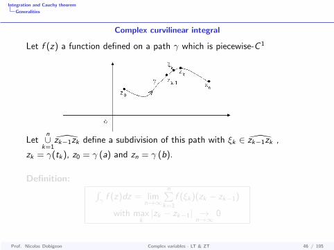
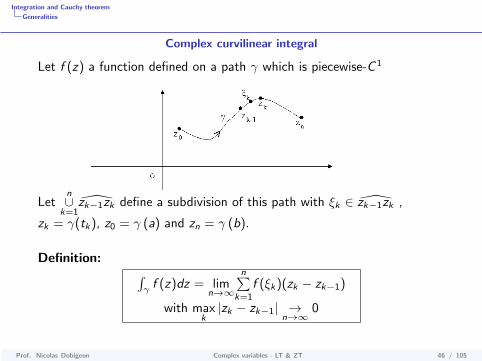
Complex curvilinear integral
Let f (z) a function defined on a path γ which is piecewise-C 1
Letn∪
k=1zk−1zk define a subdivision of this path with ξk ∈ zk−1zk ,
zk = γ(tk), z0 = γ (a) and zn = γ (b).
Definition: ∫γf (z)dz = lim
n→∞
n∑k=1
f (ξk)(zk − zk−1)
with maxk|zk − zk−1| →
n→∞0
Prof. Nicolas Dobigeon Complex variables - LT & ZT 46 / 105
Integration and Cauchy theorem
Generalities
Complex curvilinear integral
Let f (z) a function defined on a path γ which is piecewise-C 1
Letn∪
k=1zk−1zk define a subdivision of this path with ξk ∈ zk−1zk ,
zk = γ(tk), z0 = γ (a) and zn = γ (b).
Definition: ∫γf (z)dz = lim
n→∞
n∑k=1
f (ξk)(zk − zk−1)
with maxk|zk − zk−1| →
n→∞0
Prof. Nicolas Dobigeon Complex variables - LT & ZT 46 / 105

Integration and Cauchy theorem
Generalities
Complex curvilinear integral
With the following notations
zk = xk + iyk
zk − zk−1 = ∆xk + i∆yk
ξk = ak + ibk
f (ξk) = P(ak , bk) + iQ(ak , bk)
it yields ∫γf (z)dz = lim
n→∞
n∑k=1
P(ak , bk)∆xk − Q(ak , bk)∆yk
+i limn→+∞
n∑k=1
Q(ak , bk)∆xk + P(ak , bk)∆yk
with maxk|∆xk | → 0 and max
k|∆yk | → 0. Hence∫
γ
f (z)dz =
∫γ
(Pdx − Qdy) + i
∫γ
(Qdx + Pdy)
Prof. Nicolas Dobigeon Complex variables - LT & ZT 47 / 105
Integration and Cauchy theorem
Generalities
Complex curvilinear integral
Sufficient condition of existence
P and Q continious on γor f continious on γ
In practice: γ is parametrized∫γf (z)dz =
∫ b
af (γ (t)) γ′ (t) dt
Usual paths
I Line segment parallel to the X-axis,z = x + iy0, x ∈ [x1, x2]
I Line segment parallel to the Y-axis,z = x0 + iy , y ∈ [y1, y2]
I Arc of radius R0
z = R0eiθ, θ ∈ [θ1, θ2]
I Line segment coming from the originz = ρe iθ0 , ρ ∈ [ρ1, ρ2]
Prof. Nicolas Dobigeon Complex variables - LT & ZT 48 / 105
Integration and Cauchy theorem
Generalities
Complex curvilinear integral
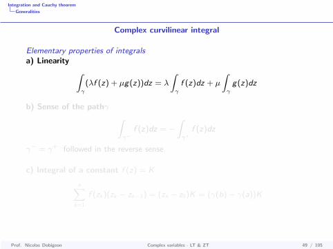
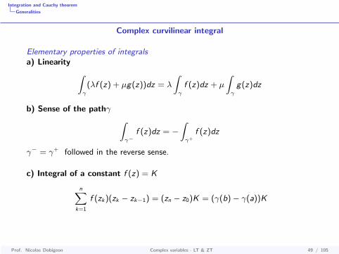
Elementary properties of integralsa) Linearity ∫
γ
(λf (z) + µg(z))dz = λ
∫γ
f (z)dz + µ
∫γ
g(z)dz
b) Sense of the pathγ ∫γ−
f (z)dz = −∫γ+
f (z)dz
γ− = γ+ followed in the reverse sense.
c) Integral of a constant f (z) = K
n∑k=1
f (zk)(zk − zk−1) = (zn − z0)K = (γ(b)− γ(a))K
Prof. Nicolas Dobigeon Complex variables - LT & ZT 49 / 105

Integration and Cauchy theorem
Generalities
Complex curvilinear integral
Elementary properties of integralsa) Linearity ∫
γ
(λf (z) + µg(z))dz = λ
∫γ
f (z)dz + µ
∫γ
g(z)dz
b) Sense of the pathγ ∫γ−
f (z)dz = −∫γ+
f (z)dz
γ− = γ+ followed in the reverse sense.
c) Integral of a constant f (z) = K
n∑k=1
f (zk)(zk − zk−1) = (zn − z0)K = (γ(b)− γ(a))K
Prof. Nicolas Dobigeon Complex variables - LT & ZT 49 / 105
Integration and Cauchy theorem
Jordan lemmas
Outline
Some Generalities
Usual functions
Holomorphic functions
Integration and Cauchy theoremGeneralitiesJordan lemmasIntegral of holomorphic functions
Residue theorem
Laplace transform
Z transform
Prof. Nicolas Dobigeon Complex variables - LT & ZT 50 / 105

Integration and Cauchy theorem
Jordan lemmas
Jordan lemmas1st Lemma Jordan
AssumptionsCr (a, r) arc of center a and radius rlimr→0( resp. ∞) supCr
|(z − a) f (z)| = 0
Conclusion
limr→0( resp. ∞)
∫Crf (z)dz = 0
Proof: ∣∣∣∣∫Cr
f (z)dz
∣∣∣∣ =
∣∣∣∣∣∫ β
α
f (a + re iθ)rie iθdθ
∣∣∣∣∣6
∫ β
α
∣∣rf (a + re iθ)∣∣ dθ
6 (β − α) supCr
|(z − a) f (z)|
Prof. Nicolas Dobigeon Complex variables - LT & ZT 51 / 105

Integration and Cauchy theorem
Jordan lemmas
Jordan lemmas2nd Jordan lemmas
Assumptionlim∞ supCr
|f (z)| = 0
Conclusions
lim∞∫Cre imz f (z)dz = 0 pour m > 0 et Cr = C+
r
lim∞∫Cre imz f (z)dz = 0 pour m < 0 et Cr = C−r
lim∞∫Cremz f (z)dz = 0 pour m < 0 et Cr = C d
r
lim∞∫Cremz f (z)dz = 0 pour m > 0 et Cr = C g
r
Proof:
|Ir | =
∣∣∣∣∫Cr
e imz f (z)dz
∣∣∣∣ =
∣∣∣∣∫ π
0
e imre iθ f (re iθ)ire iθdθ
∣∣∣∣≤ 2r sup
Cr
|f (z)|∫ π
2
0
e−mr sin θdθ
≤ supCr
|f (z)| πm
(1− e−mr ) (car sin θ >2θ
π)
Prof. Nicolas Dobigeon Complex variables - LT & ZT 52 / 105

Integration and Cauchy theorem
Integral of holomorphic functions
Outline
Some Generalities
Usual functions
Holomorphic functions
Integration and Cauchy theoremGeneralitiesJordan lemmasIntegral of holomorphic functions
Residue theorem
Laplace transform
Z transform
Prof. Nicolas Dobigeon Complex variables - LT & ZT 53 / 105

Integration and Cauchy theorem
Integral of holomorphic functions
Cauchy theorem1-connected (or simply connected) domain
Assumptionsf holomorphic on Ω, non-null open space of CLet D ⊂ Ω define a simply-connected domain of contour C
Conclusion ∫Cf (z)dz = 0
Proof (by the use of the Green-Riemann formula)∫C+
Adx + Bdy =
∫ ∫D
(∂B
∂x− ∂A
∂y
)dxdy
Prof. Nicolas Dobigeon Complex variables - LT & ZT 54 / 105
Integration and Cauchy theorem
Integral of holomorphic functions
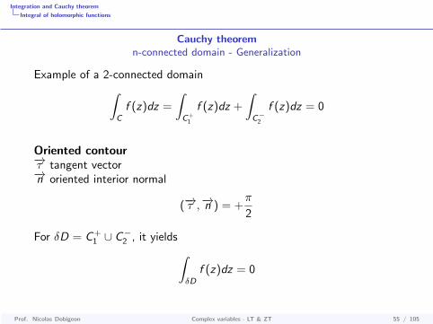
Cauchy theoremn-connected domain - Generalization
Example of a 2-connected domain∫C
f (z)dz =
∫C+
1
f (z)dz +
∫C−
2
f (z)dz = 0
Oriented contour−→τ tangent vector−→n oriented interior normal
(−→τ ,−→n ) = +π
2
For δD = C+1 ∪ C−2 , it yields∫
δD
f (z)dz = 0
Prof. Nicolas Dobigeon Complex variables - LT & ZT 55 / 105
Integration and Cauchy theorem
Integral of holomorphic functions
Cauchy theoremApplication
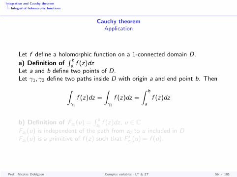
Let f define a holomorphic function on a 1-connected domain D.
a) Definition of∫ b
af (z)dz
Let a and b define two points of D.Let γ1, γ2 define two paths inside D with origin a and end point b. Then∫
γ1
f (z)dz =
∫γ2
f (z)dz =
∫ b
a
f (z)dz
b) Definition of Fz0 (u) =∫ u
z0f (z)dz , u ∈ C
Fz0 (u) is independent of the path from z0 to u included in DFz0 (u) is a primitive of f (z) such that F ′z0
(u) = f (u).
Prof. Nicolas Dobigeon Complex variables - LT & ZT 56 / 105

Integration and Cauchy theorem
Integral of holomorphic functions
Cauchy theoremApplication
Let f define a holomorphic function on a 1-connected domain D.
a) Definition of∫ b
af (z)dz
Let a and b define two points of D.Let γ1, γ2 define two paths inside D with origin a and end point b. Then∫
γ1
f (z)dz =
∫γ2
f (z)dz =
∫ b
a
f (z)dz
b) Definition of Fz0 (u) =∫ u
z0f (z)dz , u ∈ C
Fz0 (u) is independent of the path from z0 to u included in DFz0 (u) is a primitive of f (z) such that F ′z0
(u) = f (u).
Prof. Nicolas Dobigeon Complex variables - LT & ZT 56 / 105

Residue theorem
Outline
Some Generalities
Usual functions
Holomorphic functions
Integration and Cauchy theorem
Residue theoremTheorem for a bounded domain DApplication to integral calculusApplication to the sum of a series
Laplace transform
Z transform
Prof. Nicolas Dobigeon Complex variables - LT & ZT 57 / 105

Residue theorem
Theorem for a bounded domain D
Outline
Some Generalities
Usual functions
Holomorphic functions
Integration and Cauchy theorem
Residue theoremTheorem for a bounded domain DApplication to integral calculusApplication to the sum of a series
Laplace transform
Z transform
Prof. Nicolas Dobigeon Complex variables - LT & ZT 58 / 105

Residue theorem
Theorem for a bounded domain D
Residue theorem
Assumptions
I f holomorphic on Ω\ ∪jzj , Ω non-empty open set of C
I zj isolated singularities of f
I D ⊂ Ω 1-connected domain of contour ∂D inside Ω
Conclusion ∫∂D+ f (z)dz = 2iπ
∑zj∈D
resf (zj)
with (definition of resf (zj)) :
resf (zj) = limr→0
12iπ
∫C+(zj ,r)
f (z)dz
Prof. Nicolas Dobigeon Complex variables - LT & ZT 59 / 105
Residue theorem
Theorem for a bounded domain D
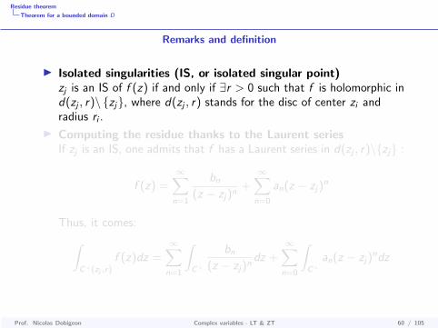
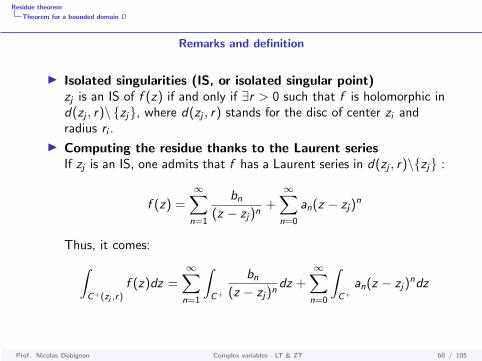
Remarks and definition
I Isolated singularities (IS, or isolated singular point)zj is an IS of f (z) if and only if ∃r > 0 such that f is holomorphic ind(zj , r)\ zj, where d(zj , r) stands for the disc of center zi andradius ri .
I Computing the residue thanks to the Laurent seriesIf zj is an IS, one admits that f has a Laurent series in d(zj , r)\zj :
f (z) =∞∑n=1
bn(z − zj)n
+∞∑n=0
an(z − zj)n
Thus, it comes:∫C+(zj ,r)
f (z)dz =∞∑n=1
∫C+
bn(z − zj)n
dz +∞∑n=0
∫C+
an(z − zj)ndz
Prof. Nicolas Dobigeon Complex variables - LT & ZT 60 / 105
Residue theorem
Theorem for a bounded domain D
Remarks and definition
I Isolated singularities (IS, or isolated singular point)zj is an IS of f (z) if and only if ∃r > 0 such that f is holomorphic ind(zj , r)\ zj, where d(zj , r) stands for the disc of center zi andradius ri .
I Computing the residue thanks to the Laurent seriesIf zj is an IS, one admits that f has a Laurent series in d(zj , r)\zj :
f (z) =∞∑n=1
bn(z − zj)n
+∞∑n=0
an(z − zj)n
Thus, it comes:∫C+(zj ,r)
f (z)dz =∞∑n=1
∫C+
bn(z − zj)n
dz +∞∑n=0
∫C+
an(z − zj)ndz
Prof. Nicolas Dobigeon Complex variables - LT & ZT 60 / 105

Residue theorem
Theorem for a bounded domain D
Remarks and definition
We set z − zj = re iθ and it yields
∞∑n=1
∫ 2π
0
bnidθ
rn−1e i(n−1)θ+ i
∞∑n=0
∫ 2π
0
anrn+1e i(n+1)θdθ
All the integrals are null (straightforward...) except:∫ 2π
0
bnidθ
rn−1e i(n−1)θwith n = 1
Thus : ∫C+(zj ,r)
f (z)dz =
∫ 2π
0
b1idθ = 2iπb1
Conclusion : resf (zj) is the coefficient of the term 1z−zj of the main
part of the Laurent series of f .
Prof. Nicolas Dobigeon Complex variables - LT & ZT 61 / 105

Residue theorem
Theorem for a bounded domain D
Remarks and definitionI Computing the residue in case of a pole of order p
One computes the Taylor series of ϕ(z) = (z − zj)pf (z) which is
holomorphic in V (zj)
ϕ(z) = ϕ(zj) + ...+(z − zj)
p−1
(p − 1)!ϕ
(p−1)(zj )
+ ...
As a consequence, the Laurent series of f is:
f (z) =ϕ(zj)
(z − zj)p+ ...+
ϕ(p−1)(zj )
(p − 1)!(z − zj)+ ...
thus
resf (zj) = 1(p−1)!ϕ
(p−1)(zj )
= 1(p−1)!
dp−1
dzp−1 [(z − zj)pf (z)]
∣∣∣z=zj
In practice:I for p > 2, one compute the Laurent series,I for p = 2, one can use resf (zj) = d
dz (z − zj)2f (z)
∣∣z=zj
,
I for p = 1, one has resf (zj) = limz→zj
(z − zj)f (z)
Prof. Nicolas Dobigeon Complex variables - LT & ZT 62 / 105
Residue theorem
Theorem for a bounded domain D
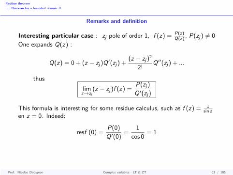
Remarks and definition
Interesting particular case : zj pole of order 1, f (z) = P(z)Q(z) , P(zj) 6= 0
One expands Q(z) :
Q(z) = 0 + (z − zj)Q′(zj) +
(z − zj)2
2!Q ′′(zj) + ...
thus
limz→zj
(z − zj)f (z) =P(zj)
Q ′(zj)
This formula is interesting for some residue calculus, such as f (z) = 1sin z
en z = 0. Indeed:
resf (0) =P(0)
Q ′(0)=
1
cos 0= 1
Prof. Nicolas Dobigeon Complex variables - LT & ZT 63 / 105
Residue theorem
Application to integral calculus
Outline
Some Generalities
Usual functions
Holomorphic functions
Integration and Cauchy theorem
Residue theoremTheorem for a bounded domain DApplication to integral calculusApplication to the sum of a series
Laplace transform
Z transform
Prof. Nicolas Dobigeon Complex variables - LT & ZT 64 / 105

Residue theorem
Application to integral calculus
Integrals of the form: I =∫∞−∞ f (x)dx
Very often, one defines f (z) and the contour which consists of a straightline associated with I and a circular parts which close path. Example:
Computing
I =
∫ +∞
−∞
x2 + 1
x4 + 1dx
Prof. Nicolas Dobigeon Complex variables - LT & ZT 65 / 105
Residue theorem
Application to integral calculus
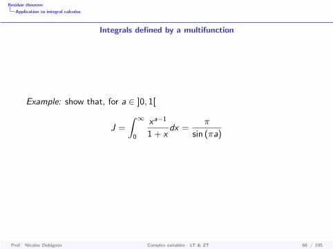
Integrals defined by a multifunction
Example: show that, for a ∈ ]0, 1[
J =
∫ ∞0
xa−1
1 + xdx =
π
sin (πa)
Prof. Nicolas Dobigeon Complex variables - LT & ZT 66 / 105

Residue theorem
Application to integral calculus
Trigonometric integrals
I =
∫ 2π
0
R(cos θ, sin θ)dθ
where R is a rational fraction. One sets z = e iθ and one derives cos θand sin θ as functions of z .It consists of computing an integral on the unit circle.Example : show that
J =
∫ 2π
0
dθ
5 + 3 sin θ=π
2
Prof. Nicolas Dobigeon Complex variables - LT & ZT 67 / 105

Residue theorem
Application to the sum of a series
Outline
Some Generalities
Usual functions
Holomorphic functions
Integration and Cauchy theorem
Residue theoremTheorem for a bounded domain DApplication to integral calculusApplication to the sum of a series
Laplace transform
Z transform
Prof. Nicolas Dobigeon Complex variables - LT & ZT 68 / 105

Residue theorem
Application to the sum of a series
Application to the sum of a series
See exercise session.
Prof. Nicolas Dobigeon Complex variables - LT & ZT 69 / 105
Laplace transform
Outline
Some Generalities
Usual functions
Holomorphic functions
Integration and Cauchy theorem
Residue theorem
Laplace transformDefinitionPropertiesInverse Laplace transformApplications
Z transform
Prof. Nicolas Dobigeon Complex variables - LT & ZT 70 / 105

Laplace transform
Definition
Outline
Some Generalities
Usual functions
Holomorphic functions
Integration and Cauchy theorem
Residue theorem
Laplace transformDefinitionPropertiesInverse Laplace transformApplications
Z transform
Prof. Nicolas Dobigeon Complex variables - LT & ZT 71 / 105

Laplace transform
Definition
Definition
Set of the (Laplace) transformable functionsE is the set of the functions f defined on R+ such that• f is locally integrable, i.e.,
∫ A
0f (t)dt <∞,∀A
• It exists x0 such that∫∞
0e−x0t f (t)dt <∞
Laplace transformFor f ∈ E , one defines its Laplace transform as
F (p) ,∫∞
0e−pt f (t)dt p ∈ C
Notation: F (p) = TL(f (t))
Prof. Nicolas Dobigeon Complex variables - LT & ZT 72 / 105

Laplace transform
Definition
DefinitionConvergences
(simple) Convergence
Thereom 1If F (p) exists for p = p0 = x0 + iy0 thenF (p) exists ∀p such that Rep > Rep0 = x0
Consequence : x ∈ R,F (p) <∞ admits a lower bound denoted xc andcalled abscissa of (simple) convergence of F .
Absolute convergence
Theorem 2If∫∞
0
∣∣e−pt f (t)∣∣ dt exists for p = p0 = x0 + iy0 then∫∞
0
∣∣e−pt f (t)∣∣ dt exists ∀p such that Rep > Rep0 = x0
Consequence :x ∈ R,
∫∞0
∣∣e−pt f (t)∣∣ dt <∞ admits a lower bound denoted
xca and called abscissa of absolute convergence of F (obviously, xc ≤ xca)
Example: f (t) = ekt sin[ekt], k > 0, xc = 0 and xca = k.
Remark : one often has xc = xca.
Prof. Nicolas Dobigeon Complex variables - LT & ZT 73 / 105

Laplace transform
Definition
Definition
Fundamental theoremIf f (t) is piecewise continuous on R+,then F (p) =
∫∞0
e−pt f (t)dt is holomorphic on ]xc ,+∞[ andthen it is infinitely differentiable on ]xc ,+∞[ with
dnF (p)dpn =
∫∞0
dn
dpn [e−pt f (t)] dt
Consequence: deriving xc from F (p)
If F (p) a function of the complex variable p is the Laplace transformof a function f (t) which admits isolated singularities skand branching points rj in C, then xc = supRe(sk , rj)
Examples: F (p) = 1p(p−2) xc = 2
F (p) = 1p+1 xc = 0
Prof. Nicolas Dobigeon Complex variables - LT & ZT 74 / 105

Laplace transform
Properties
Outline
Some Generalities
Usual functions
Holomorphic functions
Integration and Cauchy theorem
Residue theorem
Laplace transformDefinitionPropertiesInverse Laplace transformApplications
Z transform
Prof. Nicolas Dobigeon Complex variables - LT & ZT 75 / 105
Laplace transform
Properties
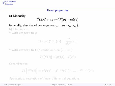
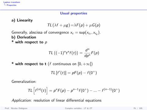
Usual properties
a) LinearityTL (λf + µg) =λF (p) + µG (p)
Generally, abscissa of convergence xc = sup(xcf , xcg ).b) Derivation* with respect to p
TL (−1)ntnf (t) =dn
dpnF (p)
* with respect to t (f continuous on [0,+∞[)
TL [f ′(t)] = pF (p)− f (0+)
Generalization:
TL[f (n)(t)
]= pnF (p)− pn−1f (0+)− ...− f (n−1)(0+)
Application: resolution of linear differential equations
Prof. Nicolas Dobigeon Complex variables - LT & ZT 76 / 105
Laplace transform
Properties
Usual properties
a) LinearityTL (λf + µg) =λF (p) + µG (p)
Generally, abscissa of convergence xc = sup(xcf , xcg ).b) Derivation* with respect to p
TL (−1)ntnf (t) =dn
dpnF (p)
* with respect to t (f continuous on [0,+∞[)
TL [f ′(t)] = pF (p)− f (0+)
Generalization:
TL[f (n)(t)
]= pnF (p)− pn−1f (0+)− ...− f (n−1)(0+)
Application: resolution of linear differential equations
Prof. Nicolas Dobigeon Complex variables - LT & ZT 76 / 105

Laplace transform
Properties
Usual properties
c) Integration* LT of a primitive
TL
[∫ t
0
f (u)du
]=
F (p)
p
Abscissa of convergence: sup(xc , 0)* Primitive of a LT
TL
[f (t)
t
]=
∫ ∞p
F (u)du
Prof. Nicolas Dobigeon Complex variables - LT & ZT 77 / 105
Laplace transform
Properties
Usual properties
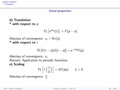
d) Translation* with respect to p
TL[eat f (t)
]= F (p − a)
Abscissa of convergence: xc + Re(a)* with respect to t
TL [f (t − a)U(t − a)] = e−apF (p)
Abscissa of convergence: xcRemark: Application to periodic functionse) Scaling
TL[f( tk
)]= kF (kp) k > 0
Abscissa of convergence: xck
Prof. Nicolas Dobigeon Complex variables - LT & ZT 78 / 105

Laplace transform
Properties
Usual properties
f) Convolution
TL
[∫ t
0
f (u)g(t − u)du
]= F (p)G (p)
g) Theorems of the initial and final values
limt→0+
f (t) = limp→∞
pF (p)
limt→∞
f (t) = limp→0
pF (p)
h) Transform of seriesSeries of general term an
tn
n!with abscissa of convergence Rc =∞
TL[∑∞
n=1 antn
n!
]=∑∞
n=1an
pn+1
Example: show that TL[
sinωtt
]= Arctg ωp
Use two methods: series expansion and TL[x(t)t
]Prof. Nicolas Dobigeon Complex variables - LT & ZT 79 / 105

Laplace transform
Properties
Some Laplace transforms
Function TL ConvergenceU(t) 1
p xc = 0
eαt 1p−α xc = Reα
e iωt 1p−iω xc = 0
ch (αt) pp2−α2 xc = supRe(α,−α)
sh (αt) αp2−α2 xc = supRe(α,−α)
cosωt pp2+ω2 xc = 0
sinωt ωp2+ω2 xc = 0
t 1p2 xc = 0
tn, n ∈ N n!pn+1 xc = 0
tα, α ∈ R Γ(α+1)pα+1
with Γ(x) =∫∞
0e−ttx−1dt et Γ(n + 1) = nΓ(n) = n!
Prof. Nicolas Dobigeon Complex variables - LT & ZT 80 / 105
Laplace transform
Inverse Laplace transform
Outline
Some Generalities
Usual functions
Holomorphic functions
Integration and Cauchy theorem
Residue theorem
Laplace transformDefinitionPropertiesInverse Laplace transformApplications
Z transform
Prof. Nicolas Dobigeon Complex variables - LT & ZT 81 / 105

Laplace transform
Inverse Laplace transform
Inversion formula
X (p) =
∫ ∞0
x(t)e−ptdt =
∫ ∞0
x(t)e−ate−j2πftdt
with p = a + j2πfAnalogy with the Fourier transform
X (f ) = TF (x(t)) =∫R x(t)e−j2πft
x(t) = TF−1(X (f )) =∫R X (f )e+j2πftdf
Hence :
X (p) = TF[x(t)e−atU(t)
]and thus the inversion formula:
x(t)U(t) = 12iπ
∫D↑ X (p)eptdp
One applies the residue theorem with X (p)ept .Example: X (p) = 1√
p
Prof. Nicolas Dobigeon Complex variables - LT & ZT 82 / 105
Laplace transform
Applications
Outline
Some Generalities
Usual functions
Holomorphic functions
Integration and Cauchy theorem
Residue theorem
Laplace transformDefinitionPropertiesInverse Laplace transformApplications
Z transform
Prof. Nicolas Dobigeon Complex variables - LT & ZT 83 / 105
Laplace transform
Applications
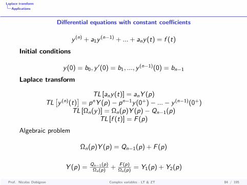
Differential equations with constant coefficients
y (n) + a1y(n−1) + ...+ any(t) = f (t)
Initial conditions
y(0) = b0, y′(0) = b1, ..., y
(n−1)(0) = bn−1
Laplace transform
TL [any(t)] = anY (p)TL[y (n)(t)
]= pnY (p)− pn−1y(0+)− ...− y (n−1)(0+)
TL [Ωn(y)] = Ωn(p)Y (p)− Qn−1(p)TL [f (t)] = F (p)
Algebraic problem
Ωn(p)Y (p) = Qn−1(p) + F (p)
Y (p) = Qn−1(p)Ωn(p) + F (p)
Ωn(p) = Y1(p) + Y2(p)
Prof. Nicolas Dobigeon Complex variables - LT & ZT 84 / 105

Laplace transform
Applications
Differential equations with constant coefficients
a) Y1(p) Algebraic fraction
Y1(p) =Qn−1(p)∏r
i=1(p − pi )ki
where pi is a ki -order root with∑r
i=1 ki = nPartial fraction decomposition :
Y1(p) =r∑
i=1
Ai1
p − pi+
Ai2
(p − pi )2 + ...+
Aiki
(p − pi )ki
where
y1(t) =∑r
i=1 epi t[Ai1 + Ai2t + ...+ Aiki t
ki−1]
b) Y2(p) = F (p)Ωn(p) = F (p)× 1
Ωn(p) thus:
y2(t) =
∫ t
0
f (u)Rn(t − u)du
Hence, the solution of the problem is y(t) = y1(t) + y2(t)Prof. Nicolas Dobigeon Complex variables - LT & ZT 85 / 105
Laplace transform
Applications
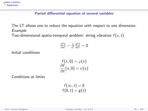
Partial differential equation of several variables
The LT allows one to reduce the equation with respect to one dimension.Example:Two-dimensional spatio-temporal problem: string vibration f (x , t)
∂2f∂x2 − 1
c2∂2f∂t2 = 0
Initial conditions
f (x , 0) = ϕ(x)∂f
∂t(x , 0) = ψ(x)
Conditions at limits
f (∞, t) = 0f (0, t) = g(t)
Prof. Nicolas Dobigeon Complex variables - LT & ZT 86 / 105

Laplace transform
Applications
Partial differential equation of several variables
Solution thanks to the LT (p is a considered as a parameter)
F (x , p) =
∫ ∞0
e−pt f (x , t)dt
TL
[∂f
∂t
]= pF (x , p)− f (x , 0)
= pF (x , p)− ϕ(x)
TL
[∂2f
∂t2(x , t)
]= p2F (x , p)− pf (x , 0)− ∂f
∂t(x , 0)
= p2F (x , p)− pϕ(x)− ψ(x)
TL
[∂2f
∂x2(x , t)
]=
∫ ∞0
e−pt∂2f (x , t)
∂x2dt
=∂2
∂x2
∫ ∞0
e−pt f (x , t)dt =d2F (x , p)
dx2
Prof. Nicolas Dobigeon Complex variables - LT & ZT 87 / 105

Laplace transform
Applications
Partial differential equation of several variables
One obtains
d2F (x,p)dx2 − p2F (x , p) = pϕ(x) + ψ(x)
with
F (∞, p) = TL [f (∞, t)] = 0
G (p) = TL [g(t)] = TL[f (0, t)] = F (0, p)
One-dimensional problem (differential equations + conditions at limits).
Prof. Nicolas Dobigeon Complex variables - LT & ZT 88 / 105

Z transform
Outline
Some Generalities
Usual functions
Holomorphic functions
Integration and Cauchy theorem
Residue theorem
Laplace transform
Z transformDefinitionPropertiesInverse Z transformApplicationsLaplace and Z transforms
Prof. Nicolas Dobigeon Complex variables - LT & ZT 89 / 105
Z transform
Definition
Outline
Some Generalities
Usual functions
Holomorphic functions
Integration and Cauchy theorem
Residue theorem
Laplace transform
Z transformDefinitionPropertiesInverse Z transformApplicationsLaplace and Z transforms
Prof. Nicolas Dobigeon Complex variables - LT & ZT 90 / 105
Z transform
Definition
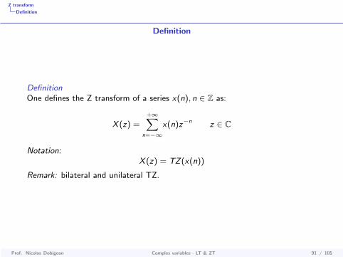
Definition
DefinitionOne defines the Z transform of a series x(n), n ∈ Z as:
X (z) =+∞∑
n=−∞
x(n)z−n z ∈ C
Notation:X (z) = TZ(x(n))
Remark: bilateral and unilateral TZ.
Prof. Nicolas Dobigeon Complex variables - LT & ZT 91 / 105

Z transform
Definition
Definition
Domain of convergenceThe domain of convergence is the set of complex numbers z such that theseries X (z) converges.
Reminder: Cauchy criterion
limn→+∞
n√|un| < 1 =⇒
+∞∑n=0
un converge
One has a sufficient condition of convergence. Thanks to this criterion, oneshows that the series X (z) converges once:
0 ≤ R−x < |z | < R+x ≤ +∞
Example: X (z) =∑+∞
n=0 z−n converges for |z | > 1
Prof. Nicolas Dobigeon Complex variables - LT & ZT 92 / 105

Z transform
Properties
Outline
Some Generalities
Usual functions
Holomorphic functions
Integration and Cauchy theorem
Residue theorem
Laplace transform
Z transformDefinitionPropertiesInverse Z transformApplicationsLaplace and Z transforms
Prof. Nicolas Dobigeon Complex variables - LT & ZT 93 / 105
Z transform
Properties
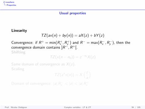
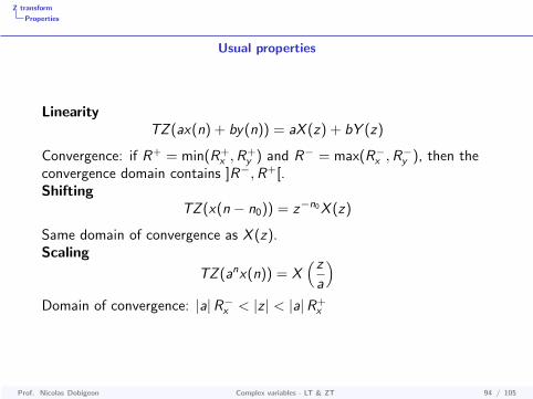
Usual properties
LinearityTZ (ax(n) + by(n)) = aX (z) + bY (z)
Convergence: if R+ = min(R+x ,R
+y ) and R− = max(R−x ,R
−y ), then the
convergence domain contains ]R−,R+[.Shifting
TZ (x(n − n0)) = z−n0X (z)
Same domain of convergence as X (z).Scaling
TZ (anx(n)) = X(za
)Domain of convergence: |a|R−x < |z | < |a|R+
x
Prof. Nicolas Dobigeon Complex variables - LT & ZT 94 / 105

Z transform
Properties
Usual properties
LinearityTZ (ax(n) + by(n)) = aX (z) + bY (z)
Convergence: if R+ = min(R+x ,R
+y ) and R− = max(R−x ,R
−y ), then the
convergence domain contains ]R−,R+[.Shifting
TZ (x(n − n0)) = z−n0X (z)
Same domain of convergence as X (z).Scaling
TZ (anx(n)) = X(za
)Domain of convergence: |a|R−x < |z | < |a|R+
x
Prof. Nicolas Dobigeon Complex variables - LT & ZT 94 / 105
Z transform
Properties
Usual properties
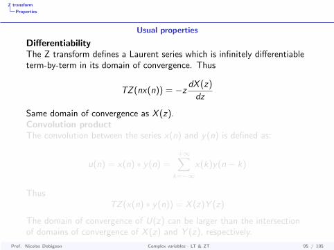
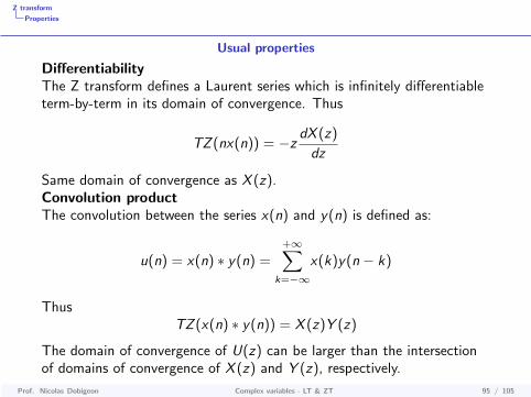
DifferentiabilityThe Z transform defines a Laurent series which is infinitely differentiableterm-by-term in its domain of convergence. Thus
TZ (nx(n)) = −z dX (z)
dz
Same domain of convergence as X (z).Convolution productThe convolution between the series x(n) and y(n) is defined as:
u(n) = x(n) ∗ y(n) =+∞∑
k=−∞
x(k)y(n − k)
ThusTZ (x(n) ∗ y(n)) = X (z)Y (z)
The domain of convergence of U(z) can be larger than the intersectionof domains of convergence of X (z) and Y (z), respectively.
Prof. Nicolas Dobigeon Complex variables - LT & ZT 95 / 105
Z transform
Properties
Usual properties
DifferentiabilityThe Z transform defines a Laurent series which is infinitely differentiableterm-by-term in its domain of convergence. Thus
TZ (nx(n)) = −z dX (z)
dz
Same domain of convergence as X (z).Convolution productThe convolution between the series x(n) and y(n) is defined as:
u(n) = x(n) ∗ y(n) =+∞∑
k=−∞
x(k)y(n − k)
ThusTZ (x(n) ∗ y(n)) = X (z)Y (z)
The domain of convergence of U(z) can be larger than the intersectionof domains of convergence of X (z) and Y (z), respectively.
Prof. Nicolas Dobigeon Complex variables - LT & ZT 95 / 105

Z transform
Inverse Z transform
Outline
Some Generalities
Usual functions
Holomorphic functions
Integration and Cauchy theorem
Residue theorem
Laplace transform
Z transformDefinitionPropertiesInverse Z transformApplicationsLaplace and Z transforms
Prof. Nicolas Dobigeon Complex variables - LT & ZT 96 / 105

Z transform
Inverse Z transform
Inverse Z transform
The inverse Z transform is given by:
x(n) =1
j2π
∫C+
X (z)zn−1dz
where C is a closed path included into the domain of convergence
Prof. Nicolas Dobigeon Complex variables - LT & ZT 97 / 105

Z transform
Inverse Z transform
TZ inverse
ProofOne has to compute the integrals
J(n, k) =
∫C+
zn−k−1dz
Thanks to the residue theorem, one shows that:
J(n, k) =
0 si n 6= kj2π si n = k
Hence:
1
j2π
∫C+
X (z)zn−1dz =1
j2π
∫C+
( ∞∑k=−∞
x(k)z−k
)zn−1dz
=1
j2π
∞∑k=−∞
x(k)J(n, k)
= x(n)
Remark : tablesProf. Nicolas Dobigeon Complex variables - LT & ZT 98 / 105
Z transform
Applications
Outline
Some Generalities
Usual functions
Holomorphic functions
Integration and Cauchy theorem
Residue theorem
Laplace transform
Z transformDefinitionPropertiesInverse Z transformApplicationsLaplace and Z transforms
Prof. Nicolas Dobigeon Complex variables - LT & ZT 99 / 105

Z transform
Applications
Discrete signal filtering
See exercise session and/or later.
Prof. Nicolas Dobigeon Complex variables - LT & ZT 100 / 105

Z transform
Applications
Recurrence relations
Example: 1-st order system
y(n)− ay(n − 1) = x(n) |a| < 1
The input of the system is chosen as:
x(n) = bnU(n) with |b| < 1
where U(n) is the Heaviside step function.
I Compute y(n) for n ≥ 0 given that y(n) = 0 for n < 0.
I Determine the impulse response of the system h(n) such thaty(n) = x(n) ∗ h(n).
Prof. Nicolas Dobigeon Complex variables - LT & ZT 101 / 105

Z transform
Laplace and Z transforms
Outline
Some Generalities
Usual functions
Holomorphic functions
Integration and Cauchy theorem
Residue theorem
Laplace transform
Z transformDefinitionPropertiesInverse Z transformApplicationsLaplace and Z transforms
Prof. Nicolas Dobigeon Complex variables - LT & ZT 102 / 105
Z transform
Laplace and Z transforms
Laplace and Z transforms
Let x(t) define a causal signal whose Laplace transform is:
X (p) =
∫ ∞0
x(t)e−ptdt
One samples this signal with period T and one denotes X (z) its Ztransform:
X (z) =∞∑n=0
x(nT )z−n
ThenX (z) =
∑res X (p)
1−epT z−1
Prof. Nicolas Dobigeon Complex variables - LT & ZT 103 / 105

Z transform
Laplace and Z transforms
Laplace and Z transforms
The formula of inverse Laplace transform provides
x(t)U(t) =1
2iπ
∫D↑
X (p)eptdp
hence
X (z) =∞∑n=0
x(nT )z−n =∞∑n=0
[1
2iπ
∫D↑
X (p)epnTdp
]z−n
=1
2iπ
∫D↑
X (p)∞∑n=0
(z−1epT
)ndp
Once∣∣z−1epT
∣∣ < 1, on a
X (z) =1
2iπ
∫D↑
X (p)1
1− z−1epTdp =
∑res
X (p)
1− epT z−1
Prof. Nicolas Dobigeon Complex variables - LT & ZT 104 / 105

Z transform
Laplace and Z transforms
Complex VariablesLaplace Transform – Z Transform
Prof. Nicolas Dobigeon
University of ToulouseIRIT/INP-ENSEEIHT
http://www.enseeiht.fr/[email protected]
Prof. Nicolas Dobigeon Complex variables - LT & ZT 105 / 105


