
Constraint Programming for LNG Ship Scheduling and
Inventory Management
V. Goela, M. Sluskyb, W.-J. van Hoevec, K. C. Furmand, Y. Shaoa
a ExxonMobil Upstream Research Company{vikas.goel,yufen.shao}@exxonmobil.com
bDepartment of Mathematical Sciences, Carnegie Mellon [email protected]
c Tepper School of Business, Carnegie Mellon [email protected]
d ExxonMobil Research and [email protected]
Abstract
We propose a constraint programming approach for the optimization of inven-tory routing in the liquefied natural gas industry. We present two constraintprogramming models that rely on a disjunctive scheduling representation ofthe problem. We also propose an iterative search heuristic to generate goodfeasible solutions for these models. Computational results on a set of large-scale test instances demonstrate that our approach can find better solutionsthan existing approaches based on mixed integer programming, while being4 to 10 times faster on average.
Keywords: Routing, Inventory, Constraint Programming
1. Introduction
Natural gas, which is primarily composed of methane, is a relatively cleanburning fuel for a number of outlets including electricity generation and heat-ing. Traditionally natural gas projects were developed near local markets ornear major pipelines. However, liquefied natural gas (LNG) provides theability to develop a natural gas project in an isolated area of the world andyet efficiently deliver that gas to market. The technology has been availablefor several decades, and it accounts for meeting a rapidly growing share ofnatural gas market demand. One of the most important advantages of LNGtanker ship over pipelines is the access it provides to markets overseas.
Preprint submitted to European Journal of Operations Research October 29, 2013
The focus of this work is on a central operational issue in the LNG indus-try: designing schedules for the ships to deliver LNG from the production(liquefaction) terminals to the demand (regasification) terminals. This is acomplex problem because it combines ship routing with inventory manage-ment at the terminals.
A primary application of this problem is to support analysis for the designof the supply chain for new projects. Typically, new LNG projects requirebuilding not only the natural gas production and treatment facilities, butalso constructing the ships and the production-side terminals, berths andstorage tanks. Operationally, a delivery schedule for each customer in theLNG supply chain is negotiated on an annual basis. The supply and demandrequirements of the sellers and purchasers are accommodated through thedevelopment of this annual delivery schedule, which is a detailed schedule ofLNG loadings, deliveries and ship movements for the planning year.
A solution to the inventory routing problem can be used in two primaryways: (1) to analyze LNG supply chain design decisions such as LNG fleetsize and composition, and terminal infrastructure during the concept anddetailed design phases for new LNG projects, and (2) to develop the deliveryschedules for operations of these LNG projects, quantify schedule inefficiency,and conduct “what-if” analysis to test how robust a schedule is to disruptionevents. Goel et al. (2012) first introduced this problem, and proposed amixed integer programming (MIP) model as well as a MIP-based heuristicfor finding good solutions. Yet, both the MIP model and the MIP heuristicsuffered from scalability issues for larger instances. This was one of the mainmotivations for studying constraint programming in the present work as analternative method for solving this problem.
The LNG inventory routing problem is a special case of the maritimeinventory routing problem. The basic maritime inventory routing problem(see (Christiansen and Fagerholt 2009)) involves the transportation of a sin-gle product from loading ports to unloading ports, with each port havinga given inventory storage capacity and a production or consumption rate,therefore combining inventory management and ship routing. These are typ-ically treated separately in much of the maritime transportation industry.In such problems, the number of visits to a port and the quantity of prod-uct to be loaded or unloaded are not predetermined. Christiansen et al.(2013) provide a recent survey in ship routing and scheduling research overthe last decade. LNG inventory routing business cases and common problem
2

characteristics are discussed by Andersson et al. (2010).Constraint Programming (CP) has been applied before to industrial rout-
ing and scheduling problems, and most CP solvers offer a specific modelinginterface for representing these problems (Baptiste et al. 2001, 2006). In par-ticular, it is common to represent routing problems as disjunctive schedulingproblems, in which a visit to a location becomes a task to be scheduled,and the distance between two locations is modeled as a ‘sequence-dependentset-up time’ between tasks. CP models can be particularly effective whenthe schedule is subject to time windows, when additional precedence rela-tions are imposed between tasks, and when finding good feasible solutions ismore important than proving optimality of a solution. One major benefit ofCP over Mixed Integer Programming (MIP) models is that CP scales muchbetter when the time granularity is increased; the CP model and associatedalgorithms are dependent on the number of tasks and resources rather thanthe number of time points.
Our CP models will use the basic structure described above, based ondisjunctive scheduling. In our case, however, the number of (optional) tasksis proportional to the number of time points, and consequently our CP modelsmay potentially still have scalability issues. Nonetheless, our CP models arestill much smaller than the corresponding MIP models. As we are mostlyinterested in finding good solutions in a reasonable amount of time, withprovable optimality as secondary goal, the investigation of the performance ofCP models on this challenging problem domain seems warranted. In fact, ourexperimental results will demonstrate that our CP models are competitivewith a dedicated heuristic for this problem, while in some cases it can findsuperior solutions. Moreover, when we apply our dedicated search heuristic,our CP approach can outperform the existing MIP-based heuristic both interms of solution quality and solving time.
This paper is organized as follows. In the next section, we present adescription of the problem under consideration. In section 3, we presentan overview of the CP terminology used in the paper. In sections 4 and 5we present two CP models. Our heuristic search algorithm is presented insection 6. Computational results to highlight the effectiveness of the proposedmodels and algorithm over existing methods on a set of large realistic testinstances are presented in section 7. Finally, conclusions and directions forfuture research are presented in section 8.
3

2. Problem Description
Every year, LNG producers develop an annual delivery schedule for eachof their customers. A delivery schedule specifies in detail when each cargowill be delivered and by what ship throughout the planned year. The annualdelivery schedule attempts to best accommodate the expected requirementsof each party for the planned year. During the plan year, the producers andcustomers seek to adhere to the agreed upon delivery schedule as closely aspossible.
In this paper, we address the combined inventory management and cargorouting problem for the delivery of liquefied natural gas (LNG) that waspresented by Goel et al. (2012). The problem can be described as follows.There is a set of liquefaction terminals with fixed storage capacities. Eachliquefaction terminal has a given production profile for the planning horizon,as well as a limited number of berths for ships to load cargo on each day.At the other end of the supply chain, there is a set of regasification (regas)terminals that have fixed storage capacities and a limited number of berthsfor ships to unload cargoes. Each regas terminal has an overall contractualLNG demand that has to be delivered over the planning horizon, and a givenbaseline consumption profile (regas rate).
The LNG is delivered using a heterogeneous fleet of ships. We restrictour attention to full-load and full-discharge problems. In other words, LNGships are always filled to their maximum capacity prior to departing an LNGterminal and are completely discharged prior to departing regasification ter-minals. Due to safety and qualification restrictions, each ship can only visit aselect (pre-specified) set of terminals. It is common for some LNG to boil-offduring a voyage. Similar to Goel et al. (2012), we assume that we know thedischarge volumes for each ship and that these amounts are independent ofvoyage, waiting times, and time of year. Loading and unloading an LNGship requires one day of operation during which a berth has to be occupied.Ships are allowed to wait outside a production (regas) terminal only beforeloading (discharging) their cargo. Ships do not occupy a berth during thisprocess.
The problem has the following goals: delivering the contracted amount ofgas to each customer and minimizing the interruptions to operations on bothsides of the supply chain during the planning horizon. Interruptions includelost production stemming from running out of storage on the production side,and stock-outs due to the lack of inventory for consumption on the demand
4

side.In this paper, we assume that the travel time between terminals is an
integer multiple of days and does not have seasonality. Also, we do notconsider variability in the regas rates.
3. Scheduling Terminology
As mentioned before, our CP models are based on applying a resourcescheduling analogy to the IRP. As we will formulate our CP model usingconcepts from IBM ILOG CPOptimizer, we next briefly introduce those con-cepts using the terminology from Laborie (2009). Specifically, we will apply‘interval variables’, ‘sequence variables’ and ‘cumul functions’.
An interval variable x is a decision variable that can be used to representa task to be scheduled over time. The domain of an interval variable is asubset of {⊥} ∪ {[s, e) | s, e ∈ Z, s ≤ e}. An interval variable is fixed if itsdomain is reduced to a singleton, i.e., either x = ⊥ which reflects that x isabsent, or x is present and x = [s, e) for some fixed s, e. Interval variablescan thus naturally represent optional tasks to be scheduled: s represents thestart time, e the end time, and e − s the length of the task if it is present.In our application, we use interval variables to represent the loading anddischarging of ships at the terminals.
We will apply the following expressions for interval variables. Here, xrepresents an interval variable and A a set of interval variables.
• lengthOf(x) returns the length of x, i.e., e− s if x = [s, e),
• presenceOf(x) returns whether x is present (true) or absent (false),
• startOf(x, t) returns the start of x if it is present, and value t if x isabsent,
• Alternative(x,A) models an exclusive alternative among elements inA. If x is present, then exactly one element of A is present and xstarts and ends together with this specific element. Interval variable xis absent if and only if all elements in A are absent.
The expressions lengthOf(x), presenceOf(x), and startOf(x, t) can be usedin a model to define or constrain the respective attributes of x. They canalso be used to impose conditions on other constraints. The expressionAlternative(x,A) represents an ‘alternative resource’ constraint that can
5
be used, for example, to identify the machine at which a task is to be exe-cuted.
A sequence variable p is defined on a set of interval variables A. A valuefor p is a permutation of all present intervals of A. It can be used to rep-resent a disjunctive resource, for which tasks cannot overlap in time. Theno-overlap requirement also allows us to model sequence-dependent setuptimes between tasks. To this end, we associate each interval a ∈ A with aninteger ‘type’ θ(p, a), and define the transition distance between two typesas a function M : N × N → Z. That is, for two interval variables a andb, M(θ(p, a), θ(p, b)) expresses the minimal distance between the end of aand the start of b relative to the sequence variable p. For example, typesmay represent the color of a paint activity for a painting machine (in whichcase the transition time represents the cleaning time between different col-ors), or the geographic location of an activity in routing problems (in whichcase the transition time represents the distance between two activities). Theno-overlap constraint can then be defined as NoOverlap(p,M). In our ap-plication, we use sequence variables to represent the sequence of tasks, andhence the route, to be performed by a ship.
We will apply the following expressions for sequence variables. Here, prepresents a sequence variable, x represents an interval variable, and A a setof interval variables.
• SequenceVar(A, θ) defines a sequence variable over A with type map θ,1
• First(p, x) constrains x to be the first interval variable of p, if present,
• typeOfNext(p, x, j1, j2) returns the type of the interval variable that isnext to x in sequence p, value j1 if x is the last interval variable of p,and value j2 if x is absent (argument j2 is optional and can be omittedif x is always present).
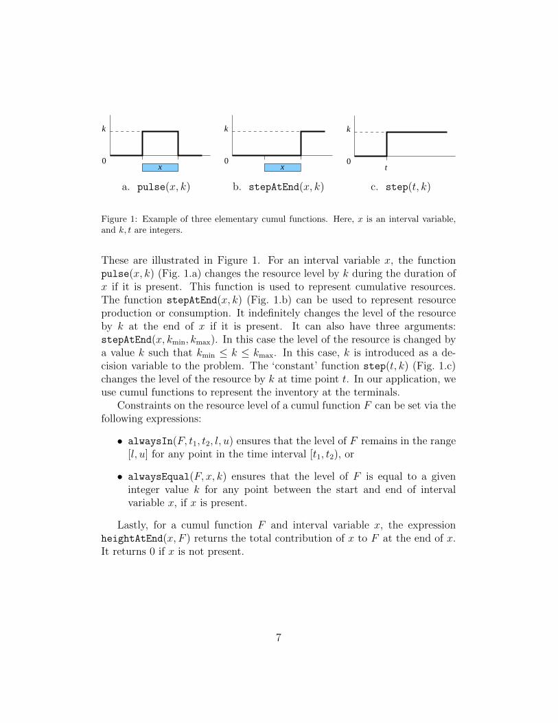
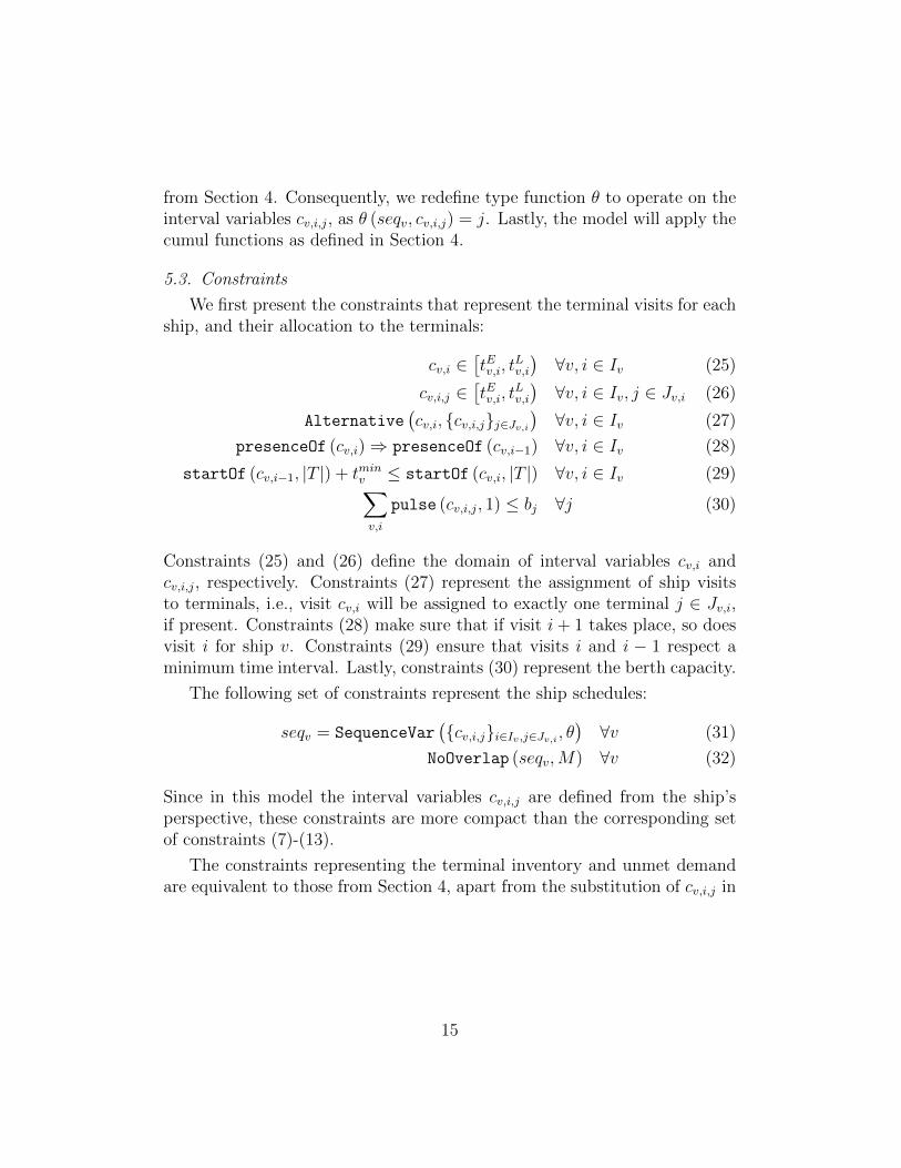
A cumul function can be used to represent (and constrain) the usagelevel of a resource over time. It aggregates individual contributions of in-terval variables, which are represented by elementary cumul functions. Inthis work, we apply the elementary functions pulse, stepAtEnd, and step.
1We note that both CPOptimizer and OPL do not have a compact definition for se-quence variables. We therefore introduce the shorthand SequenceVar, to concisely repre-sent our models.
6
x0
k
x0
k
0
k
t
a. pulse(x, k) b. stepAtEnd(x, k) c. step(t, k)
Figure 1: Example of three elementary cumul functions. Here, x is an interval variable,and k, t are integers.
These are illustrated in Figure 1. For an interval variable x, the functionpulse(x, k) (Fig. 1.a) changes the resource level by k during the duration ofx if it is present. This function is used to represent cumulative resources.The function stepAtEnd(x, k) (Fig. 1.b) can be used to represent resourceproduction or consumption. It indefinitely changes the level of the resourceby k at the end of x if it is present. It can also have three arguments:stepAtEnd(x, kmin, kmax). In this case the level of the resource is changed bya value k such that kmin ≤ k ≤ kmax. In this case, k is introduced as a de-cision variable to the problem. The ‘constant’ function step(t, k) (Fig. 1.c)changes the level of the resource by k at time point t. In our application, weuse cumul functions to represent the inventory at the terminals.
Constraints on the resource level of a cumul function F can be set via thefollowing expressions:
• alwaysIn(F, t1, t2, l, u) ensures that the level of F remains in the range[l, u] for any point in the time interval [t1, t2), or
• alwaysEqual(F, x, k) ensures that the level of F is equal to a giveninteger value k for any point between the start and end of intervalvariable x, if x is present.
Lastly, for a cumul function F and interval variable x, the expressionheightAtEnd(x, F ) returns the total contribution of x to F at the end of x.It returns 0 if x is not present.
7
4. CP1: Constraint Programming Model with Terminal CargoEnumeration
In our first CP model, the tasks to be scheduled will correspond to thecargoes to be loaded at the production terminals, and the cargoes to bedischarged at the regas terminals. We will collectively refer to these tasksas cargoes, and to both production and regas terminals simply as terminals.Each ship defines a disjunctive resource (tasks cannot overlap in time), as wellas a production/consumption resource representing its inventory. Likewise,the inventory for each terminal is represented by a production/consumptionresource.
Each terminal is seeking for its tasks to be executed (scheduled), whileeach task can be executed by at most one ship. This leads to a CP modelwith optional tasks (the cargoes) and alternative resources. Namely, we needto allocate each cargo to at most one ship, and we don’t know in advancehow many cargoes will be executed in total. We note that cargo sizes aredetermined implicitly through the assignment of cargoes to ships.
We next introduce the notation that will be used in our models.
8
4.1. Sets and Parameters
L Set of production (liquefaction) terminals (integer)
R Set of regasification terminals (integer)
J Set of all terminals, J = L ∪RT Set of days (planning horizon), T = {1, 2, . . . , |T |}Dj Total demand for LNG over planning horizon at terminal j ∈ RIj Set of possible cargoes to be loaded/discharged at terminal j
V Set of ships (vessels)
pj,t Daily production rate at terminal j ∈ L at time t
dj,t Daily regasification rate at terminal j ∈ R at time t
g0j Initial inventory at terminal j
γj Storage capacity at terminal j
γv,j Volume loaded/discharged by ship v at terminal j
tEj,i, tLj,i ith cargo at terminal j has time window
[tEj,i, t
Lj,i
]tEj,i,v, t
Lj,i,v ith cargo at terminal j for ship v has time window
[tEj,i,v, t
Lj,i,v
]τj Minimum delay between successive cargoes at terminal j
M(j, j′) Travel time from terminal j to terminal j′, including port time
j0v Initial terminal of ship v
t0v Time from which ship v is available
bj Number of berths at terminal j
JDj,v Terminals that ship v can depart to after visiting terminal j
wDj penalty for unmet demand at terminal j ∈ Rwj,t penalty for lost production/stockout at terminal j at time t
We also introduce the integer set Ij := {1, 2, . . . } to represent the possiblecargoes for terminal j. The size of this set depends on the production rate(resp. regasification rate) of the terminal and the time horizon. In ourmodel, we will assume that if cargo i is scheduled, then also cargo i − 1 isscheduled (for i > 1). Therefore, the time windows for the cargoes i ∈ Ij arepreprocessed so that tEj,i, t
Lj,i ≤ |T | and tEj,i,v, t
Lj,i,v ≤ |T | for all j, i ∈ Ij, v ∈ V .
4.2. Variables and Cumul Functions
Interval variables:
9

cj,i ith cargo at terminal j, for i ∈ Ijcj,i,v ith cargo at terminal j using ship v, for i ∈ Ijav unavailability of ship v before arrival at its initial destination
sltj,t loss in time slot t at terminal j (present if there is loss at t)
slt2j,t present if sltj,t is present, and it immediately succeeds sltj,t
Here, loss refers to lost production for liquefaction terminals or stockout forregas terminals. The interval variable slt2j,t will be used in our model torepresent that whenever a loss occurs, the resource must be at its bound inthe next time slot.
All these interval variables except av are optional, i.e., they can be eitherpresent or absent, and have a fixed size of 1 (one time slot). Interval variableav is always present for each ship v ∈ V : it will be the first activity for shipv, with fixed length [1, t0v).
Sequence variables and parameters:
seqv collects interval variables assigned to ship v
θ type function θ (seqv, cj,i,v) = j, θ (seqv, av) = j0v
Here, the type θ of an interval variable is its location, i.e., the function θmaps each interval to the location of its terminal. The type of interval av isthe vessel’s starting position j0v .
Integer variables:
lj,t loss at terminal j in time slot t
Recall that loss refers to lost production for liquefaction terminals or stockoutfor regas terminals.
10
Cumul functions:
p̃j cumulative production over time at terminal j ∈ Ld̃j cumulative regasification over time at terminal j ∈ Rz̃j cumulative volume loaded (discharged) over time at terminal j ∈ Jl̃j cumulative loss (lost production or stockout) over time at terminal j ∈ J
4.3. Constraints
We first introduce constraints to represent the cargoes at each terminal,and the ships to handle them:
cj,i ∈[tEj,i, t
Lj,i + 1
)∀j, i ∈ Ij (1)
cj,i,v ∈[tEj,i,v, t
Lj,i,v + 1
)∀j, i ∈ Ij, v (2)
Alternative(cj,i, {cj,i,v}v) ∀j, i ∈ Ij (3)
presenceOf (cj,i)⇒ presenceOf (cj,i−1) ∀j, i ∈ Ij (4)
startOf (cj,i−1, |T |) + τj ≤ startOf (cj,i, |T |+ τj) ∀j, i ∈ Ij (5)∑i
pulse (cj,i, 1) ≤ bj ∀j (6)
Constraints (1) and (2) define the domains of the variables cj,i and cj,i,v,respectively. Constraints (3) represent the assignment of terminal cargoesto ships, i.e., exactly one ship will execute cargo cj,i, if present. Constraints(4) ensure that if the ith cargo is present at terminal j, so is the (i − 1)th
cargo. Constraints (5) ensure the proper ordering, and minimum delay τ ,for all consecutive cargoes at a terminal. Recall that the second argument inthe function startOf is the value returned if the interval variable is absent.Lastly, constraints (6) ensures that the number of cargoes scheduled at eachtime point at a terminal does not exceed the number of berths.
The following set of constraints represent the ship schedules:
av ∈[1, t0v
)∀v (7)
lengthOf(av) = t0v − 1 ∀v (8)
seqv = SequenceVar(av ∪ {cj,i,v}j,i∈Ij , θ
)∀v (9)
First (seqv, av) ∀v (10)
typeOfNext(seqv, av, φ
1)in{j0v , φ
1}∀v (11)
11
typeOfNext(seqv, cj,i,v, φ
1, φ2)in JDj,v ∪
{φ1, φ2
}∀j, i ∈ Ij, v (12)
NoOverlap (seqv,M) ∀v (13)
Constraints (7) define the domains of variables av, while constraints (8) definethe associated sizes. Constraints (9) define the sequence variable seqv overits associated interval variables and types, for each ship v. The first activityof ship v must be av, as defined by constraints (10). The next two sets ofconstraints (11) and (12) limit the locations that can be visited after theinitial location j0v , respectively cargo at location j. Here, φ1 is a dummyvalue returned by typeOfNext for a last task completed by a ship, and φ2 isa dummy value returned by typeOfNext for absent interval variables. Thelast constraint set (13) ensures that the interval variables do not overlap intime, and respect the transition times (distance) between locations.
Formally, by introducing types φ1 and φ2, we need to extend the definitionof the transition matrix M . We do this as M (j, φ1) = 1, M (j, φ2) = 0.
The following set of constraints represent the terminal inventory and un-met demand:
sltj,t ∈ [t, t+ 1) ∀j ∈ J, t ∈ T (14)
p̃j =∑t
step (t+ 1, pj,t) ∀j ∈ L (15)
d̃j =∑t
step (t+ 1, dj,t) ∀j ∈ R (16)
z̃j =∑v
∑i∈Ij
stepAtEnd (cj,i,v, γv,j) ∀j ∈ J (17)
l̃j =∑t
stepAtEnd (sltj,t, 1, lj,t) ∀j ∈ J (18)
alwaysIn(step
(1, g0j
)+ p̃j − z̃j − l̃j, 1, |T |, 0, γj
)∀j ∈ L (19)
alwaysIn(step
(1, g0j
)− d̃j + z̃j + l̃j, 1, |T |, 0, γj
)∀j ∈ R (20)
Constraints (14) define the domain of the interval variable sltj,t that rep-resents the loss at terminal j in time slot t. Constraints (15), (16), and(17) define cumul functions for the daily production, daily demand, andloading/discharge of cargo at the terminals. Constraints (18) represent thecumul function for the loss over time at terminal j. These are all added
12
together, with the starting inventory g0j , to form the overall inventory levelof each terminal; in constraints (19) and (20) these levels are constrained tobe in the range [0, γj] for each terminal j. Note that the production andregasification terminals are handled separately.
In principle, the constraints (14)-(20) are sufficient to define the inven-tory aspect of the problem. However, the constraint propagation related tothe interval variables representing the loss can be improved by adding thefollowing redundant ‘complementarity’ constraints. These constraints repre-sent that whenever a loss occurs, the resource must be at its lower bound(for regasification terminals) or its upper bound (for liquefaction terminals).To this end, we introduce a new optional interval variable slt2j,t that willrepresent that during time slot t + 1 following a loss in slot t, the resourcelevel is at its respective bound:
slt2j,t ∈ [t+ 1, t+ 2) ∀j ∈ J, t ∈ T (21)
presenceOf (sltj,t) = presenceOf (slt2j,t) ∀j ∈ J, t ∈ T (22)
alwaysEqual(step
(1, g0j
)+ p̃j − z̃j − l̃j, slt2j,t, γj
)∀j ∈ L (23)
alwaysEqual(step
(1, g0j
)− d̃j + z̃j + l̃j, slt2j,t, 0
)∀j ∈ R (24)
Constraints (21) define the domain and size of the interval variable slt2j,t.Constraints (22) ensure that variables sltj,t and slt2j,t are both present orabsent. Constraints (23) and (24) ensure that the resource level of j is equalto γj for liquefaction terminals and 0 for regasification terminals whenever aloss occurs at time slot t.
Lastly, we state the objective function as follows:
minimize∑j∈R
wDj · max
0, Dj −∑v,i∈Ij
γv,j · presenceOf (cj,i,v)
+∑j∈J
∑t
wj,t · heightAtEnd(sltt, l̃j
)Here, the first term represents the penalty for under-delivery, weighted bywDj for regasification terminal j ∈ R. The second term represents the penaltyfor lost production and stockout, weighted by wj,t for terminal j ∈ J andtime point t ∈ T .
13

5. CP2: Constraint Programming Model with Ship Visit Enumer-ation
In the previous section, we defined cargoes from the perspective of theterminals. Here, we present an alternative CP model following from a ‘dual’perspective, that of the ships. For each ship, we enumerate a maximal set ofterminal visits that it can execute within the planning horizon. Each visitto a terminal corresponds to a task in a scheduling problem. The terminalscorrespond to resources. Each ship is seeking for its tasks to be executed.The constraint that a ship should travel from a production terminal to a regasterminal and vice versa is implicitly captured by restricting the domains ofthe variables. Cargo sizes are determined implicitly based on the ship for theassociated task.
5.1. Sets and Parameters
We will re-apply the sets and parameters from Section 4.1. In addition,we need the following:
Iv set of possible terminal visits for ship v
Jv set of terminals compatible with ship v
Jv,i if visit i = 1, Jv,i = {j0v}.if i is odd ≥ 1 and j0v is a production terminal, Jv,i = Jv ∩ Lif i is odd ≥ 1 and j0v is regas terminal, Jv,i = Jv ∩Rif i is even and j0v is a production terminal, Jv,i = Jv ∩Rif i is even and j0v is a regas terminal, Jv,i = Jv ∩ L
tEv,i earliest time ith terminal visit for ship v can take place
tminv minimum travel time between any production and any regas terminal
at which ship v is allowed
5.2. Variables and Cumul Functions
The main change from the model in Section 4 is the definition of theinterval variables. We now apply the following interval variables:
cv,i ith terminal visit for ship v, for i ∈ Ivcv,i,j ith terminal visit for ship v at terminal j, for i ∈ Iv, j ∈ Jv,i
All these interval variables are optional and have a fixed size of 1 (one timeslot). In addition, the model will apply interval variables sltj,t and slt2j,tas defined in Section 4. The model will also apply sequence variable seqv
14
from Section 4. Consequently, we redefine type function θ to operate on theinterval variables cv,i,j, as θ (seqv, cv,i,j) = j. Lastly, the model will apply thecumul functions as defined in Section 4.
5.3. Constraints
We first present the constraints that represent the terminal visits for eachship, and their allocation to the terminals:
cv,i ∈[tEv,i, t
Lv,i
)∀v, i ∈ Iv (25)
cv,i,j ∈[tEv,i, t
Lv,i
)∀v, i ∈ Iv, j ∈ Jv,i (26)
Alternative(cv,i, {cv,i,j}j∈Jv,i
)∀v, i ∈ Iv (27)
presenceOf (cv,i)⇒ presenceOf (cv,i−1) ∀v, i ∈ Iv (28)
startOf (cv,i−1, |T |) + tminv ≤ startOf (cv,i, |T |) ∀v, i ∈ Iv (29)∑v,i
pulse (cv,i,j, 1) ≤ bj ∀j (30)
Constraints (25) and (26) define the domain of interval variables cv,i andcv,i,j, respectively. Constraints (27) represent the assignment of ship visitsto terminals, i.e., visit cv,i will be assigned to exactly one terminal j ∈ Jv,i,if present. Constraints (28) make sure that if visit i+ 1 takes place, so doesvisit i for ship v. Constraints (29) ensure that visits i and i − 1 respect aminimum time interval. Lastly, constraints (30) represent the berth capacity.
The following set of constraints represent the ship schedules:
seqv = SequenceVar({cv,i,j}i∈Iv ,j∈Jv,i , θ
)∀v (31)
NoOverlap (seqv,M) ∀v (32)
Since in this model the interval variables cv,i,j are defined from the ship’sperspective, these constraints are more compact than the corresponding setof constraints (7)-(13).
The constraints representing the terminal inventory and unmet demandare equivalent to those from Section 4, apart from the substitution of cv,i,j in
15
the cumul function definition of z̃j:
sltj,t ∈ [t, t+ 1) ∀j ∈ J, t ∈ T (33)
p̃j =∑t
step (t+ 1, pj,t) ∀j ∈ L (34)
d̃j =∑t
step (t+ 1, dj,t) ∀j ∈ R (35)
z̃j =∑v
∑i∈Ij
stepAtEnd (cv,i,j, γv,j) ∀j ∈ J (36)
l̃j =∑t
stepAtEnd (sltj,t, 1, lj,t) ∀j ∈ J (37)
alwaysIn(step
(1, g0j
)+ p̃j − z̃j − l̃j, 1, |T |, 0, γj
)∀j ∈ L (38)
alwaysIn(step
(1, g0j
)− d̃j + z̃j + l̃j, 1, |T |, 0, γj
)∀j ∈ R (39)
Similar to the previous model, we can apply the complementarity constraints(21)-(24) to improve the propagation of the loss variables.
The objective function is stated as:
minimize∑j∈R
wDj · max
0, Dj −∑
(v,i)|j∈Jv,i
γv,j · presenceOf (cv,i,j)
+∑j∈J
∑t
wj,t · heightAtEnd(sltt, l̃j
)
6. Cumulative Volume Lower Bound Based Search
In this section, we present a heuristic method to generate good feasi-ble solutions for models CP1 and CP2. The proposed algorithm is basedon the insight that the overall objective for the problem will be minimizedif we maximize loadings at the production terminal, and discharges at theregas terminals such that the loads and discharges take place at regular in-tervals. Such a schedule will minimize the likelihood of violating inventoryconstraints, and maximize the likelihood of delivering the contractual vol-umes to the regas terminals.
Let zj,t represent the cumulative volume loaded (discharged) at produc-tion (regas) terminal j until t. Let lj,t and gj,t represent the loss and inventory,
16

respectively, at terminal j at time t. We have
gj,t = g0j +∑t′≤t
(pj,t′ − lj,t′)− zj,t ∀j ∈ L, t ∈ T (40)
If the total lost production over the entire planning horizon at productionterminal j is λj, we have∑
t′≤t
lj,t′ ≤ λj ∀j ∈ L, t ∈ T. (41)
Together with the inventory capacity constraints gj,t ≤ γj,∀j ∈ L, t ∈ T , itfollows that
zj,t ≥ g0j − γj +∑t′≤t
pj,t′ − λj ∀j ∈ L, t ∈ T (42)
In the context of our constraint programming models, inequality (42) can bemodeled as follows
z̃j ≥ step(1, g0j − γj − λj
)+ p̃j ∀j ∈ L (43)
Observe that the time dependency is implicit in the CP formulation, sincez̃j and p̃j are cumul functions over the time horizon T .
Similarly, if λj is the total stockout over the planning horizon for regasterminal j, we can show that
zj,t ≥ −g0j +∑t′≤t
dj,t′ − λj ∀j ∈ R, t ∈ T (44)
Inequality (44) can be modeled in our CP models as follows
z̃j ≥ step(1,−g0j − λj
)+ d̃j ∀j ∈ R (45)
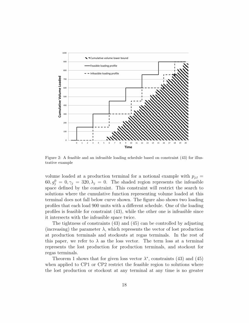
As we will demonstrate with Theorem 1, constraints (43) and (45) not onlylimit the total losses at terminal j to be no greater than λj, but also forcethe model to limit the search to solutions where loadings and discharges ata terminal take place at “regular” intervals by enforcing a lower limit on thevolume loaded or discharged at each terminal at each time period. Figure2 illustrates the cumulative lower bound implied by constraint (43) on the
17
0
100
200
300
400
500
600
700
800
900
1000
0 1 2 3 4 5 6 7 8 9 10 11 12 13 14 15 16 17 18 19 20
Cum
ulat
ive
Volu
me
Load
ed
Time
Cumulative volume lower bound
Feasible loading profile
Infeasible loading profile
Figure 2: A feasible and an infeasible loading schedule based on constraint (43) for illus-trative example
volume loaded at a production terminal for a notional example with pj,t =60, g0j = 0, γj = 320, λj = 0. The shaded region represents the infeasiblespace defined by the constraint. This constraint will restrict the search tosolutions where the cumulative function representing volume loaded at thisterminal does not fall below curve shown. The figure also shows two loadingprofiles that each load 900 units with a different schedule. One of the loadingprofiles is feasible for constraint (43), while the other one is infeasible sinceit intersects with the infeasible space twice.
The tightness of constraints (43) and (45) can be controlled by adjusting(increasing) the parameter λ, which represents the vector of lost productionat production terminals and stockouts at regas terminals. In the rest ofthis paper, we refer to λ as the loss vector. The term loss at a terminalrepresents the lost production for production terminals, and stockout forregas terminals.
Theorem 1 shows that for given loss vector λ∗, constraints (43) and (45)when applied to CP1 or CP2 restrict the feasible region to solutions wherethe lost production or stockout at any terminal at any time is no greater
18
than that in the solution defined by λ∗.
Theorem 1. Let λ∗ represent the loss vector for a solution to model CP1(or CP2). There does not exist a feasible solution to CP1 (or CP2) with lossvector λs such that ∃j ∈ (L ∪ R), λsj > λ∗j and that satisfies constraints (43)and (45) as defined for λ = λ∗.
Proof. We prove the theorem for CP1 by contradiction. The proof for CP2is similar. Suppose there exists a solution to CP1 that satisfies constraints(43) and (45) defined for λ = λ∗. Further, suppose that the solution has aloss vector λs, such that for terminal j ∈ L, λsj > λ∗j (the proof for the casewhere j ∈ R is similar).
Let λsj = λ∗j + ε where ε > 0. Let z̃sj and l̃sj represent the values for the
cumulative functions z̃j and l̃j, respectively, in the solution under considera-tion.
From (43) we have
z̃sj ≥ step(1, g0j − γj − λ∗j
)+ p̃j
Equivalently, we have
z̃sj ≥ step(1, g0j
)− step (1, γj)− step
(1, λ∗j
)+ p̃j (46)
Let us define the cumulative function g̃sj to represent the inventory intank for terminal j in the solution under consideration. By definition
g̃sj = step(1, g0j
)+ p̃j − z̃sj − l̃sj (47)
Combining (46) and (47), we get
g̃sj + l̃sj ≤ step (1, γj) + step(1, λ∗j
)(48)
We use the notation F |t to indicate the value of a cumul function F attime t. Let
ts = min{t | l̃sj
∣∣∣t
= λsj
}. (49)
By definition of l̃sj , l̃sj
∣∣∣|T |
= λsj . Hence, such ts exists.
Considering (48) at ts, we have
g̃sj∣∣ts
+ l̃sj
∣∣∣ts≤ γj + λ∗j
19
Since l̃sj
∣∣∣ts
= λsj = λ∗j + ε, we get
g̃sj∣∣ts≤ γj − ε (50)
By definition of ts, we have l̃sj
∣∣∣ts−1
< l̃sj
∣∣∣ts
. Thus, from (18) we get
presenceOf (sltj,ts) = True. Then from (22) we get presenceOf (slt2j,ts) =True. Next, from (23) we get
g0j +(p̃j − z̃j − l̃j
)∣∣∣ts
= γj
Combining this with (47), we get
g̃sj∣∣ts
= γj (51)
(50) and (51) are contradictory since ε > 0. �
The proposed cumulative volume lower bound based search is a four phasealgorithm. In phase 0, the algorithm finds a first feasible solution by solvingthe model in full space until a feasible solution is generated. At each iterationof phases 1 and 2, the algorithm limits the search to solutions such that thetotal loss at any terminal is smaller than a specified maximum value. Thismaximum loss at any terminal is set to be no greater than the loss at thatterminal in the incumbent solution. In phase 1, we set the maximum lossat each terminal to be a fraction of the total loss at the terminal in theincumbent solution. This fraction is chosen to be the same for all terminals.At each iteration in phase 2 on the other hand, we reduce the maximum lossfor only one terminal at a time. Therefore phase 1 seeks to reduce the lossesacross all terminals simultaneously while phase 2 involves seeking reductionin loss at one terminal at a time. Finally, in phase 3 the algorithm continuesto search in the region where it found the best solution until a stoppingcriterion is met.
As mentioned above, in phases 1 and 2 we seek to find progressively bettersolutions by monotonically decreasing the total loss at each terminal. If atany iteration we are unable to find a solution in the reduced space defined bythe maximum loss vector, we backtrack by choosing a less aggressive valuefor the maximum loss vector. This is achieved by setting the maximum lossvector to be a bigger fraction of the loss vector in the incumbent solution.
Note that the overall objective involves minimizing the total unmet de-
20
mand at the regas terminals in addition to minimizing loss production andstockouts. Progressively tightening constraints (43) and (45) by choosingmonotonically increasing values for λ ensures that the lost production andstockouts are monotonically decreasing, but not the overall objective. Hence,we introduce constraint (52) into the model at each iteration to exclude so-lutions that have a worse objective value than that of the incumbent (repre-sented by Φ).
∑j∈R
wDj · max
0, Dj −∑v,i∈Ij
γv,j · presenceOf (cj,i,v)
+∑j∈J
∑t
wj,t · heightAtEnd(sltt, l̃j
)≥ Φ (52)
The cumulative volume lower bound based search is presented in Algorithm1. This algorithm can be applied to both models CP1 and CP2. We refer tothe selected model simply as CP. Let CP ′(λ,Φ) represent the model obtainedby adding constraints (43), (45) and (52) to model CP, where λ and Φ rep-resent the loss vector and the objective value, respectively, in the incumbentsolution.
In algorithm 1, we use the following notation.
Φinc Objective value of the incumbent solution
λinc Loss vector in the incumbent solution
λmax Maximum loss vector used to define the search space
λprev Maximum loss vector used in last search that generated a new incumbent
ξρk Scale factor used in phase ρ to calculate λmax based on λinc
kmax Number of scale factors to consider in phases 1 and 2
7. Computational Results
In this section, we present computational results to compare the perfor-mance of the CP models and the proposed search algorithm with the MIPbased approaches of Goel et al. (2012), which represent the state of the art.All results have been obtained on a 64-bit Windows PC with two Intel Xeonquad core processors and 24 GB RAM. All MIP models are solved usingCPLEX 11.1 while all CP models are solved using CPOptimizer 12.1. Allruns on constraint programming models involved partitioning the search into
21

Algorithm 1 Cumulative Volume Lower Bound Based Search1: {Phase 0}2: Generate initial feasible solution to (CP)3: Update λinc, Φinc; λprev := λinc
4:
5: {Phase 1}6: k := 17: while k ≤ kmax do8: λmax := λinc · ξ1k9: solve CP ′
(λmax,Φinc
)10: if found solution then11: update λinc,Φinc
12: λprev := λmax
13: else14: k := k + 115: end if16: end while17:
18: {Phase 2}19: for all terminals j do20: k := 121: while k ≤ kmax do22: λmaxj := λincj · ξ2k23: for all terminals j′ 6= j do24: λmaxj′ := λincj′25: end for26: solve CP ′
(λmax,Φinc
)27: if found solution then28: update λinc,Φinc
29: λprev := λmax
30: else31: k := k + 132: end if33: end while34: end for35:
36: {Phase 3}37: λmax := λprev
38: solve CP ′(λmax,Φinc
)
22
two phases. The first search phase involved branching on the cargo intervalvariables (cj,i,v for model CP1 and cv,i,j for model CP2), while the secondsearch phase involved branching on the remaining variables.
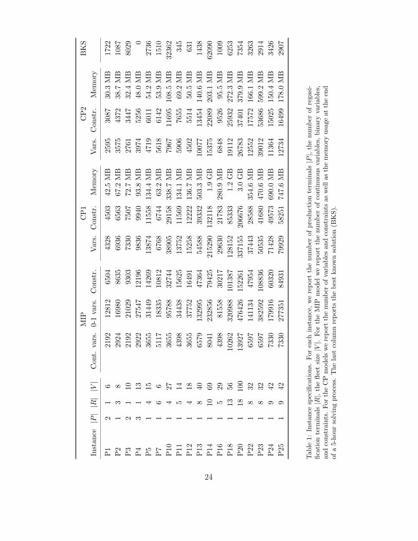
Table 1 reports the specifications for the instances used in the study.These instances reflect realistic data. Instances P1-P14 are based on theinstances presented by Goel et al. (2012). The data on some of these instanceshave minor differences compared to the instances presented by Goel et al.(2012) since we assume fixed regas rates and non-seasonal travel times inthis paper. The remaining instances are newer and in most cases, largerinstances. Table 1 reports the number of production terminals (|P |), regasterminals (|R|), ships (|V |); the number of continuous and integer variables,and the number of constraints in the MIP model; the number of variables andconstraints, and the memory usage for the constraint programming modelsCP1 and CP2 at the end of a 5 hour solve. We also report the best-knownsolution (BKS) for each instance. The table clearly emphasizes the growth inthe size of the MIP model with instance size. Note that it is not meaningful todirectly compare the sizes of the constraint programming models with thoseof the MIP model since the variable and constraint constructs in constraintprogramming internally contain much heavier data structures than the MIPmodel. However, it is clear that CP2 is significantly smaller in size thanCP1 in terms of the number of variables in constraints. This explains thescalability of CP2 compared to CP1 in terms of memory usage.
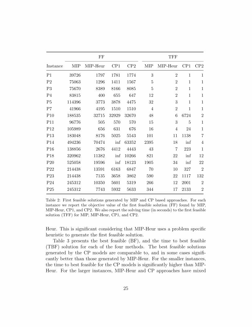
Tables 2 and 3 compare the performance of MIP and CP-based approachesin solving these instances. Specifically, we compare the performance of solv-ing the MIP model using CPLEX (referred to as MIP) with that of solvingCP1 and CP2 with CPOptimizer. All these methods are run to a 5 hourCPU limit. We also present the performance of the MIP-based heuristic(referred to as MIP-Heur) presented by Goel et al. (2012). We use the lex-icographic ordering method presented by those authors. This algorithm isrun to completion.
Table 2 presents the first feasible (FF) and the time to first feasible (TFF)solution for each of the four methods. Clearly we can observe that firstfeasible solutions generated by MIP are fairly poor, especially for the largerinstances. First feasible solutions generated by the CP models are of similaror better quality than MIP-Heur. For 3 of the largest instances, CP1 is unableto find a feasible solution. The time to first feasible for the CP models (forall instances in the case of CP2, and for the smaller instances in the case ofCP1) is also comparable or smaller than the time to first feasible for MIP-
23
MIP
CP
1C
P2
BK
S
Inst
ance|P||R||V|
Cont.
vars
.0-
1va
rs.
Con
str.
Var
s.C
onst
r.M
emor
yV
ars.
Con
str.
Mem
ory
P1
21
621
9212
812
6504
4328
4503
42.5
MB
2595
3087
30.3
MB
1722
P2
13
829
2416
980
8635
6936
6563
67.2
MB
3575
4372
38.7
MB
1087
P3
21
10
2192
2102
993
0373
3075
0772
.7M
B27
6134
4732
.4M
B80
29
P4
31
13
2922
2754
712
196
9836
9940
93.8
MB
3974
5256
48.0
MB
0
P5
14
15
3655
3144
914
269
1387
411
558
134.
4M
B47
1960
1154
.2M
B27
36
P7
16
651
1718
335
1081
267
6867
4463
.2M
B56
1861
4253
.9M
B15
10
P10
14
27
3655
9578
832
744
3890
529
158
338.
7M
B79
6711
695
108.
5M
B32
362
P11
15
14
4398
3443
815
625
1375
211
569
134.
1M
B59
0676
5569
.2M
B34
5
P12
14
18
3655
3775
216
491
1525
812
222
136.
7M
B45
0255
1450
.5M
B63
1
P13
18
40
6579
1329
9547
364
5458
839
332
503.
3M
B10
077
1345
414
0.6
MB
1438
P14
110
69
8041
2328
5679
425
2152
9013
2118
1.9
GB
1537
522
089
203.
1M
B62
090
P16
15
29
4398
8155
830
217
2963
021
783
280.
9M
B68
4895
2695
.5M
B10
09
P18
113
56
1026
232
0988
1013
8712
8152
8533
31.
2G
B19
112
2593
227
2.3
MB
6253
P20
118
100
1392
747
6426
1522
6133
7155
2066
763.
0G
B26
783
3740
137
9.9
MB
7354
P22
18
32
6597
1411
3447
954
3744
328
588
354.
6M
B12
552
1757
216
6.1
MB
3263
P23
18
32
6597
3825
9210
8836
5053
541
680
470.
6M
B39
012
5368
659
9.2
MB
2914
P24
19
42
7330
1799
1660
320
7142
849
573
690.
0M
B11
364
1502
515
0.4
MB
3426
P25
19
42
7330
2773
5184
931
7992
958
251
747.
6M
B12
734
1649
917
8.0
MB
2907
Tab
le1:
Inst
ance
spec
ifica
tion
s.F
orea
chin
stan
ce,
we
rep
ort
the
nu
mb
erof
pro
du
ctio
nte
rmin
als|P|,
the
nu
mb
erof
regasi
-fi
cati
onte
rmin
als|R|,
the
flee
tsi
ze|V|.
For
the
MIP
model
we
rep
ort
the
nu
mb
erof
conti
nu
ou
sva
riab
les,
bin
ary
vari
ab
les,
and
con
stra
ints
.F
orth
eC
Pm
od
els
we
rep
ort
the
num
ber
of
vari
ab
les
an
dco
nst
rain
tsas
wel
las
the
mem
ory
usa
ge
at
the
end
ofa
5-h
our
solv
ing
pro
cess
.T
he
last
colu
mn
rep
ort
sth
eb
est
kn
own
solu
tion
(BK
S).
24
FF TFF
Instance MIP MIP-Heur CP1 CP2 MIP MIP-Heur CP1 CP2
P1 39726 1797 1781 1774 3 2 1 1
P2 75063 1296 1411 1567 5 2 1 1
P3 75670 8389 8166 8085 5 2 1 1
P4 83815 400 655 647 12 2 1 1
P5 114396 3773 3878 4475 32 3 1 1
P7 41966 4195 1510 1510 4 2 1 1
P10 188535 32715 32929 32670 48 6 6724 2
P11 96776 505 570 570 15 3 5 1
P12 105989 656 631 676 16 4 24 1
P13 183048 8176 5025 5543 101 11 1138 7
P14 494236 70474 inf 63352 2395 18 inf 4
P16 138856 2676 4412 4443 43 7 223 1
P18 320962 11382 inf 10266 821 22 inf 12
P20 525058 19596 inf 18123 1905 34 inf 22
P22 214438 13591 6163 6847 70 10 327 2
P23 214438 7135 3658 3862 590 22 1117 132
P24 245312 10350 5601 5319 266 12 2001 2
P25 245312 7743 5932 5633 344 17 2133 2
Table 2: First feasible solutions generated by MIP and CP based approaches. For eachinstance we report the objective value of the first feasible solution (FF) found by MIP,MIP-Heur, CP1, and CP2. We also report the solving time (in seconds) to the first feasiblesolution (TFF) for MIP, MIP-Heur, CP1, and CP2.
Heur. This is significant considering that MIP-Heur uses a problem specificheuristic to generate the first feasible solution.
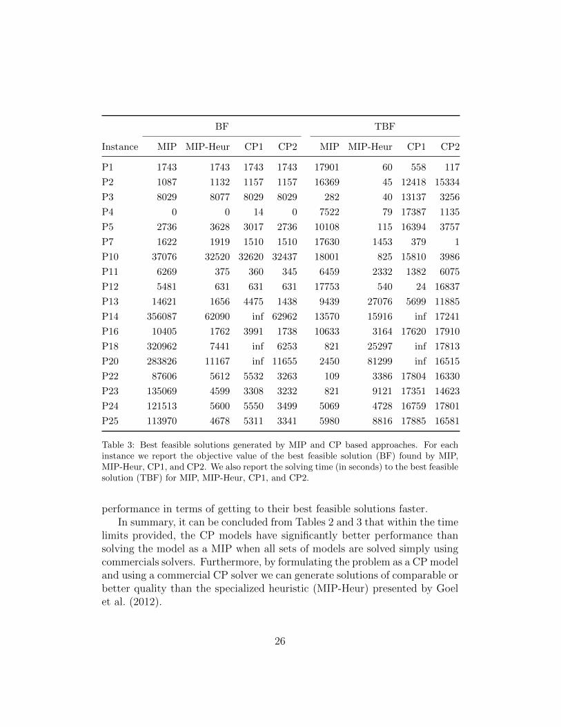
Table 3 presents the best feasible (BF), and the time to best feasible(TBF) solution for each of the four methods. The best feasible solutionsgenerated by the CP models are comparable to, and in some cases signifi-cantly better than those generated by MIP-Heur. For the smaller instances,the time to best feasible for the CP models is significantly higher than MIP-Heur. For the larger instances, MIP-Heur and CP approaches have mixed
25
BF TBF
Instance MIP MIP-Heur CP1 CP2 MIP MIP-Heur CP1 CP2
P1 1743 1743 1743 1743 17901 60 558 117
P2 1087 1132 1157 1157 16369 45 12418 15334
P3 8029 8077 8029 8029 282 40 13137 3256
P4 0 0 14 0 7522 79 17387 1135
P5 2736 3628 3017 2736 10108 115 16394 3757
P7 1622 1919 1510 1510 17630 1453 379 1
P10 37076 32520 32620 32437 18001 825 15810 3986
P11 6269 375 360 345 6459 2332 1382 6075
P12 5481 631 631 631 17753 540 24 16837
P13 14621 1656 4475 1438 9439 27076 5699 11885
P14 356087 62090 inf 62962 13570 15916 inf 17241
P16 10405 1762 3991 1738 10633 3164 17620 17910
P18 320962 7441 inf 6253 821 25297 inf 17813
P20 283826 11167 inf 11655 2450 81299 inf 16515
P22 87606 5612 5532 3263 109 3386 17804 16330
P23 135069 4599 3308 3232 821 9121 17351 14623
P24 121513 5600 5550 3499 5069 4728 16759 17801
P25 113970 4678 5311 3341 5980 8816 17885 16581
Table 3: Best feasible solutions generated by MIP and CP based approaches. For eachinstance we report the objective value of the best feasible solution (BF) found by MIP,MIP-Heur, CP1, and CP2. We also report the solving time (in seconds) to the best feasiblesolution (TBF) for MIP, MIP-Heur, CP1, and CP2.
performance in terms of getting to their best feasible solutions faster.In summary, it can be concluded from Tables 2 and 3 that within the time
limits provided, the CP models have significantly better performance thansolving the model as a MIP when all sets of models are solved simply usingcommercials solvers. Furthermore, by formulating the problem as a CP modeland using a commercial CP solver we can generate solutions of comparable orbetter quality than the specialized heuristic (MIP-Heur) presented by Goelet al. (2012).
26
Next, we evaluate the performance of the CP-based search algorithm pre-sented in this paper. We compare the performance of this method againstMIP-Heur since that is the best algorithm among the existing methods. Inthe results presented, the sub-problems solved in phases 1 and 2 of the pro-posed algorithm are terminated based on optimality, infeasibility, branchlimit and/or a solution limit, whichever comes first. At the beginning of phase2, we order the set of terminals in decreasing order of the corresponding lossesin the incumbent solution. In phase 2, we iterate through the set of terminalsin this sorted order starting from the terminal that has the largest total lossin the solution found at the end of phase 1. This enables us to search earlyin the regions with the maximum potential for improvement. For instanceswhere the first feasible solution has an objective value greater than 10,000,we choose kmax = 5. We choose ξ1 = ξ2 = [0.9, 0.95, 0.97, 0.99, 0.999]T forthese instances. For all other instances we choose kmax = 4 and ξ1 = ξ2 =[0.9, 0.95, 0.97, 0.99]T . This approach sets the desired accuracy level at 0.1%for instances with a large objective value, and at 1% for instances with arelatively smaller objective value.
We report solutions for the proposed search algorithm based on 2 differentconfigurations of the termination criteria. CP-Heur-nx-ksol refers to theconfiguration of the algorithm where sub-problems are solved with a branchlimit of (n ·
∑v |Iv|) and a solution limit of k. Similarly, CP-Heur-nx refers
to the configuration of the algorithm where sub-problems are solved with abranch limit of (n ·
∑v |Iv|) but without a solution limit.
Since the CP-based algorithms are terminated with an ad hoc time-limitwhereas MIP-Heur has a convergence based stopping criterion, we have de-signed a methodology to compare the quality of solutions obtained by theproposed search algorithm, and its speed in generating the solutions. Foreach instance, we define BCSa,b as the best common solution obtained byalgorithms a and b. Specifically, BCSa,b = max (BFa, BFb). The speed-upof algorithm a versus b is defined in terms of the times taken by the twoalgorithms to get a solution at least as good as BCSa,b.
Similarly, for each instance we define MCTTa,b as the Maximum Com-mon Total Time elapsed for algorithms a and b. Specifically, MCTTa,b =min (TBFa, TBFb). We quantify the quality of solutions obtained by al-gorithms a and b as the difference in the best solutions obtained by thesealgorithms at this common time relative to the best known solution for theinstance. Specifically, we report the gap in quality of solutions as 100·(Sa−Sb)
BKS,
where Sa and Sb represent the best solutions obtained by algorithms a and b
27
CP2 CP-Heur-4x-1sol CP-Heur-32x
P1 0.31 7.2 9
P2 0.0 1.18 0.39
P3 11 11 11
P4 0.07 1.8 0.24
P5 0.53 25.5 25.5
P7 916 916 916
P10 1.10 3.88 1.29
P11 384.67 76.93 72.13
P12 2.82 0.78 0.97
P13 2.30 1.21 6.35
P14 0.46 3.56 6.11
P16 0.25 15.84 2.25
P18 22.09 3.51 1.09
P20 2.02 1.97 6.08
P22 260.67 2.65 1.83
P23 50.42 48.58 47.54
P24 1300 1300 1300
P25 5.51 33.74 10.31
Geo mean 4.55 10.5 7.86
Table 4: Speed-up of CP based algorithms relative to MIP-Heur in reaching a commonsolution
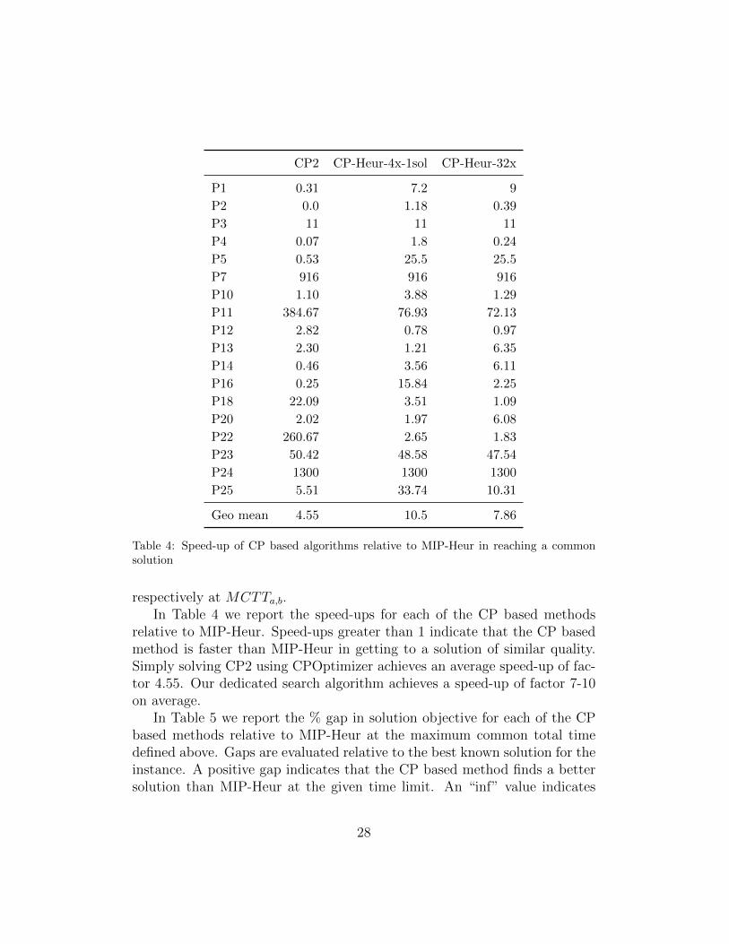
respectively at MCTTa,b.In Table 4 we report the speed-ups for each of the CP based methods
relative to MIP-Heur. Speed-ups greater than 1 indicate that the CP basedmethod is faster than MIP-Heur in getting to a solution of similar quality.Simply solving CP2 using CPOptimizer achieves an average speed-up of fac-tor 4.55. Our dedicated search algorithm achieves a speed-up of factor 7-10on average.
In Table 5 we report the % gap in solution objective for each of the CPbased methods relative to MIP-Heur at the maximum common total timedefined above. Gaps are evaluated relative to the best known solution for theinstance. A positive gap indicates that the CP based method finds a bettersolution than MIP-Heur at the given time limit. An “inf” value indicates
28

% gap relative to BKS
CP2 CP-Heur-4x-1sol CP-Heur-32x
P1 -1.34 0.41 0.93
P2 -24.2 4.14 -1.1
P3 0.31 inf inf
P4 -350 244 -393
P5 3.76 34.32 27.81
P7 inf inf inf
P10 0.21 0.32 0.47
P11 4.35 39.13 42.03
P12 0 -0.32 0
P13 17.59 45.55 101.11
P14 -1.83 2.51 13.17
P16 -1.78 66.2 65.21
P18 20.28 11.23 4.65
P20 16 26.52 57.33
P22 12.2 61.26 23.14
P23 46.6 47.53 25.29
P24 43.67 54.79 50.55
P25 30.44 15.65 60.92
Table 5: % Gap in solution quality of specified algorithm and MIP-Heur relative to bestknown solution (BKS) after a common solve time
that MIP-Heur cannot find any solution by the time (which coincides withMCTT) the CP based method terminates after successfully finding a solution.Clearly, we can see that at MCTT, solving CP2 with CPOptimizer, andthe two configurations of the proposed search algorithm provide significantlybetter solutions than MIP-Heur for the larger instances.
8. Conclusions
In this paper, we have addressed the problem of optimal LNG inventoryrouting. Most of the previous work in this area has used a mixed integerprogramming based approach. We have presented two CP models, basedon a disjunctive scheduling representation, as an alternative approach to
29
solving this problem. In addition, we have proposed an iterative heuristicsearch algorithm to generate good feasible solutions. We have shown thatwhen using leading commercial solvers, the CP-based approach generatesgood solutions much faster than a MIP based approach. Specifically, giventhe same amount of time, the CP model when solved using a commercialsolver has been shown to generate solutions of significantly higher qualitythan a specialized MIP based heuristic. Alternatively, for a given solutionquality, the CP model when solved using a commercial solver is on average4.55 times faster than the specialized MIP based heuristic. The CP basediterative heuristic is able to achieve even further improvements in speed (up toa factor 10.5 on average) and solution quality over the MIP based specializedheuristic.
References
H. Andersson, A. Hoff, M. Christiansen, G. Hasle, and A. Løkketangen. Industrialaspects and literature survey: Combined inventory management and routing.Computers and Operations Research, 37(9):1515–1536, 2010.
P. Baptiste, C. Le Pape, and W. Nuijten. Constraint-Based Scheduling: ApplyingConstraint Programming to Scheduling Problems. Kluwer Academic Publish-ers, 2001.
P. Baptiste, P. Laborie, C. Le Pape, and W. Nuijten. Constraint-based schedulingand planning. In F. Rossi, P. van Beek, and T. Walsh, editors, Handbook ofConstraint Programming, chapter 22. Elsevier, 2006.
M. Christiansen and K. Fagerholt. Maritime inventory routing problems. In C.A.Floudas and P.M. Pardalos, editors, Encyclopedia of Optimization, pages1947–1955. Springer, 2009.
M. Christiansen, K. Fagerholt, B. Nygreen, and D. Ronen. Ship routing andscheduling in the new millenium. European Journal of Operational Research,228:467–483, 2013.
V. Goel, K.C. Furman, J.-H. Song, and A.S. El-Bakry. Large neighborhood searchfor lng inventory routing. Journal of Heuristics, 18:821–848, 2012. doi:10.1007/s10732-012-9206-6.
P. Laborie. Ibm ilog cp optimizer for detailed scheduling illustrated on threeproblems. In Proceedings of CPAIOR, volume 5547 of LNCS, pages 148–162.Springer, 2009.
30


