Download - Dispersion Handout
8/22/2019 Dispersion Handout
http://slidepdf.com/reader/full/dispersion-handout 1/72
CE 524
n r 2010
1

8/22/2019 Dispersion Handout
http://slidepdf.com/reader/full/dispersion-handout 2/72
• Air pollution law in most industrial countries
based on concentration of contaminants – NAAQS in US
• ee me o o pre c concen ra ons a anygiven location
– An iven set of ollutant
– Meteorological conditions
– At any location
– For any time period
• But even best currently available concentration
2
8/22/2019 Dispersion Handout
http://slidepdf.com/reader/full/dispersion-handout 3/72
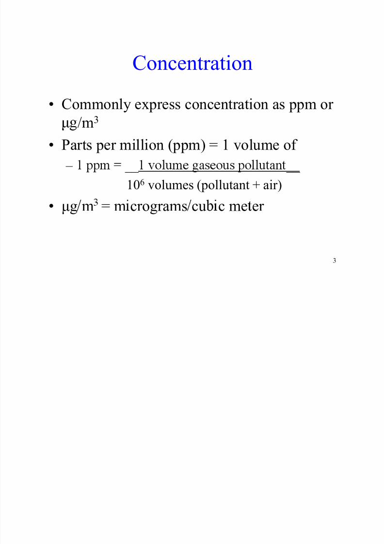
Concentration
• Commonly express concentration as ppm or /m3
• Parts per million (ppm) = 1 volume of
– __ __
106 volumes (pollutant + air)
• μg m = m crograms cu c me er
3

8/22/2019 Dispersion Handout
http://slidepdf.com/reader/full/dispersion-handout 4/72
Factors that determine Dispersion
• Physical nature of effluents•
• Meteorology• ocat on o t e stac
• Nature of terrain downwind from the stack
4
8/22/2019 Dispersion Handout
http://slidepdf.com/reader/full/dispersion-handout 5/72
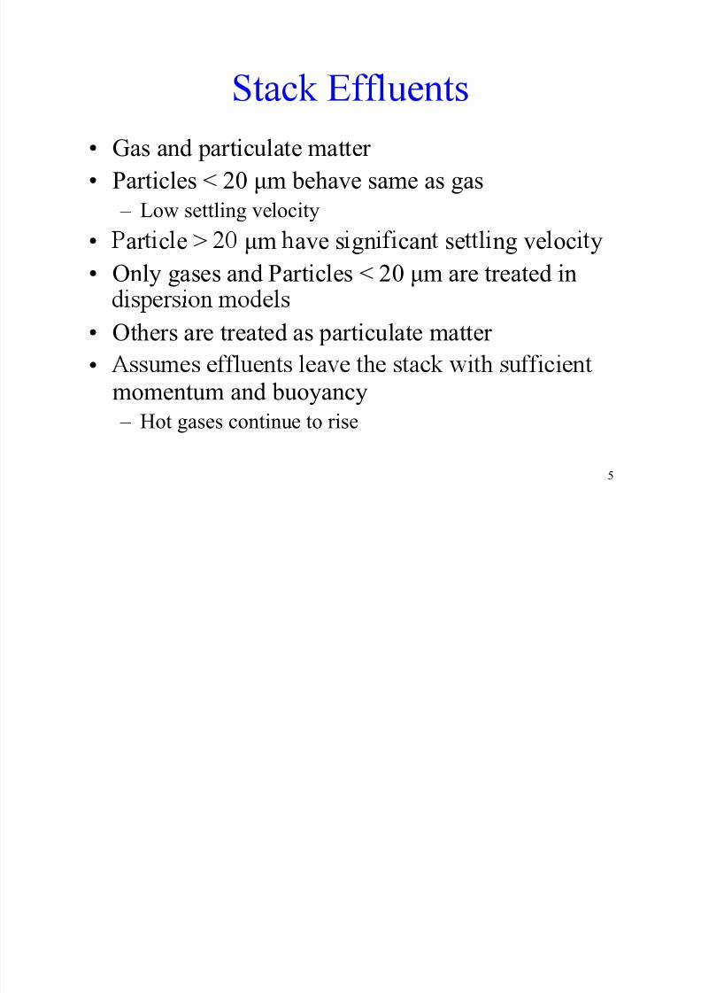
• Gas and particulate matter
• Particles < 20 μm behave same as gas – Low settling velocity
• ar c e > μm ave s gn can se ng ve oc y
• Only gases and Particles < 20 μm are treated in
• Others are treated as particulate matter
•momentum and buoyancy
– Hot gases continue to rise
5
8/22/2019 Dispersion Handout
http://slidepdf.com/reader/full/dispersion-handout 6/72
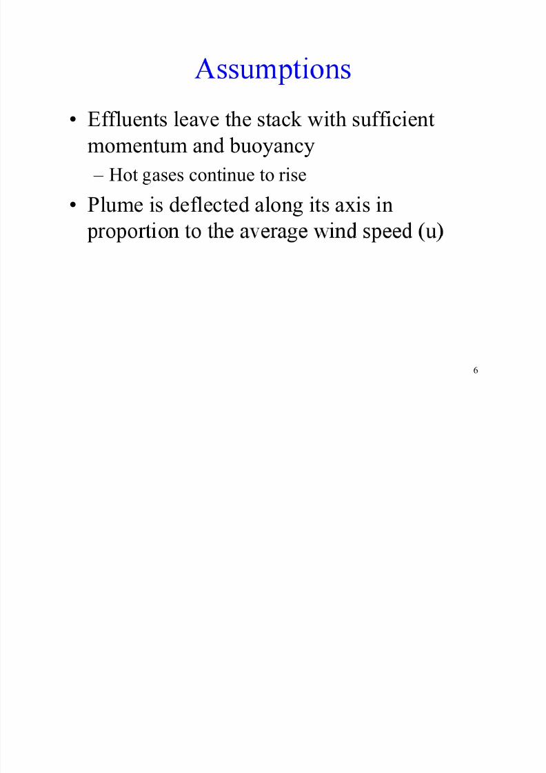
• Effluents leave the stack with sufficient
momentum and buoyancy – Hot ases continue to rise
• Plume is deflected along its axis in
6
8/22/2019 Dispersion Handout
http://slidepdf.com/reader/full/dispersion-handout 7/72
Gaussian or Normal Distribution
•
• Dispersion in y and z directions uses a
u u u -- u
• Dispersion in (x, y, z) is three-dimensional• Used to model instantaneous puff of
emissions
7
8/22/2019 Dispersion Handout
http://slidepdf.com/reader/full/dispersion-handout 8/72
Gaussian or Normal Distribution
• Pollution dispersion follows a distributionfunction
• Theoretical form: gaussian distribution
8

8/22/2019 Dispersion Handout
http://slidepdf.com/reader/full/dispersion-handout 9/72
Gaussian or Normal Distribution
• = m n f h i ri i n
• = standard deviation
context formula used to predict steady state concentration
at a point down stream
9

8/22/2019 Dispersion Handout
http://slidepdf.com/reader/full/dispersion-handout 10/72
Gaussian or Normal DistributionWhat are some properties of the normal
10f(x) becomes concentration, maximum at center of plume
8/22/2019 Dispersion Handout
http://slidepdf.com/reader/full/dispersion-handout 11/72
Gaussian or Normal distribution
• 68% of the area fall within 1 standard deviation of the mean (µ ± 1 σ).
• 95% of area fall within 1.96 standard deviation of the mean (µ ± 1.96 σ).
. of the mean (µ ± 3 σ)
11
8/22/2019 Dispersion Handout
http://slidepdf.com/reader/full/dispersion-handout 12/72
Gaussian dispersion model
• Dispersion in y and z directions aremodeled as Gaussian
• Becomes double Gaussian model
’
distribution in the x direction?
– rec on o w n
12
8/22/2019 Dispersion Handout
http://slidepdf.com/reader/full/dispersion-handout 13/72
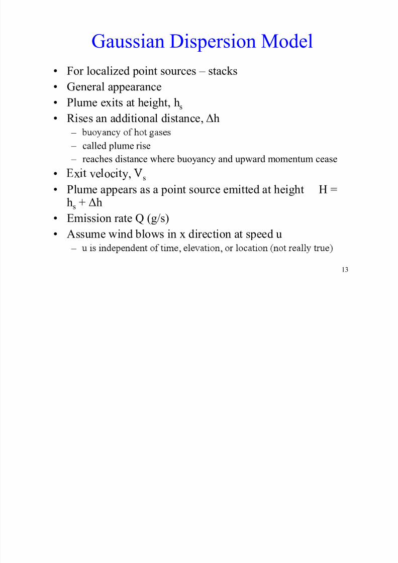
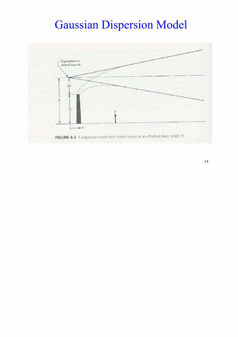
Gaussian Dispersion Model
• For localized point sources – stacks
• General appearance
• Plume exits at height, hs• Rises an additional distance, Δh
–
– called plume rise
– reaches distance where buoyancy and upward momentum cease• x ve oc y, s
• Plume appears as a point source emitted at height H =hs + Δh
• Emission rate Q (g/s)• Assume wind blows in x direction at speed u
13
– , ,
8/22/2019 Dispersion Handout
http://slidepdf.com/reader/full/dispersion-handout 14/72
Gaussian Dispersion Model
14
8/22/2019 Dispersion Handout
http://slidepdf.com/reader/full/dispersion-handout 15/72
Gaussian Dispersion Model
• Stack gas transported downstream• Dispersion in vertical direction governed by
• Dispersion in horizontal plane governed by
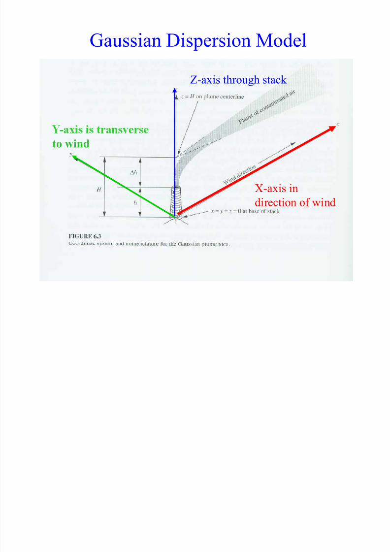
molecular and eddy diffusion• x-axis oriented to wind direction
• z-axis oriented vertically upwards
• y- rec on or en e ransverse o e w n• Concentrations are symmetric about y-axis and z-
axis
15
8/22/2019 Dispersion Handout
http://slidepdf.com/reader/full/dispersion-handout 16/72
Gaussian Dispersion Model
Z-axis through stack
-
to wind
X-axis in
direction of wind
16

8/22/2019 Dispersion Handout
http://slidepdf.com/reader/full/dispersion-handout 17/72
increase so doesdispersion
17Image source: Cooper and Alley, 2002

8/22/2019 Dispersion Handout
http://slidepdf.com/reader/full/dispersion-handout 18/72
18Image source: Cooper and Alley, 2002
8/22/2019 Dispersion Handout
http://slidepdf.com/reader/full/dispersion-handout 19/72
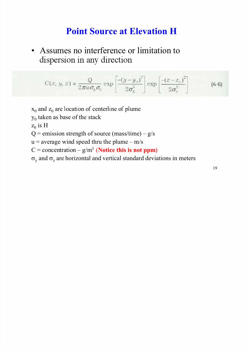
Point Source at Elevation H
• Assumes no interference or limitation to
x0 an z0 are ocat on o center ne o p ume
y0 taken as base of the stack
z0 is H
Q = emission strength of source (mass/time) – g/su = average wind speed thru the plume – m/s
C = concentration – g/m3 (Notice this is not ppm)
19
y and z are horizontal and vertical standard deviations in meters
8/22/2019 Dispersion Handout
http://slidepdf.com/reader/full/dispersion-handout 20/72
• Wind speed varies by height• International standard hei ht for wind-s eed
measurements is 10 m
• Dis ersion of ollutant is a function of windspeed at the height where pollution isemitted
• But difficult to develop relationship between height and wind speed
20
8/22/2019 Dispersion Handout
http://slidepdf.com/reader/full/dispersion-handout 21/72
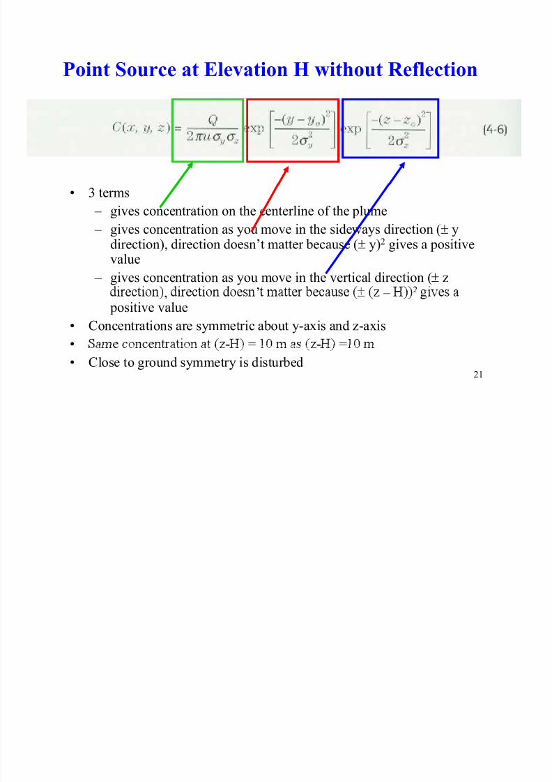
Point Source at Elevation H without Reflection
• 3 terms
– gives concentration on the centerline of the plume
– gives concentration as you move in the sideways direction ( ydirection), direction doesn’t matter because ( y)2 gives a positivevalue
– gives concentration as you move in the vertical direction ( z’ 2, –
positive value
• Concentrations are symmetric about y-axis and z-axis
• = =
21
- -
• Close to ground symmetry is disturbed

8/22/2019 Dispersion Handout
http://slidepdf.com/reader/full/dispersion-handout 22/72
reflection
• Equation 4-6 reduces to
Note in the book there are 2 equation 4-8s
22
This is the first one
8/22/2019 Dispersion Handout
http://slidepdf.com/reader/full/dispersion-handout 23/72
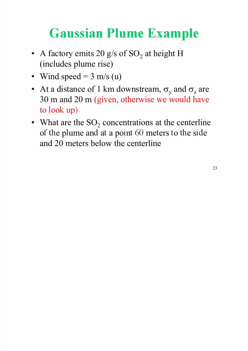
• A factory emits 20 g/s of SO2 at height H
(includes plume rise)
• Wind speed = 3 m/s (u)
• At a distance of 1 km downstream, y and z are
30 m and 20 m (given, otherwise we would haveto oo up
• What are the SO2 concentrations at the centerline
o e p ume an a a po n me ers o e s eand 20 meters below the centerline
23
8/22/2019 Dispersion Handout
http://slidepdf.com/reader/full/dispersion-handout 24/72
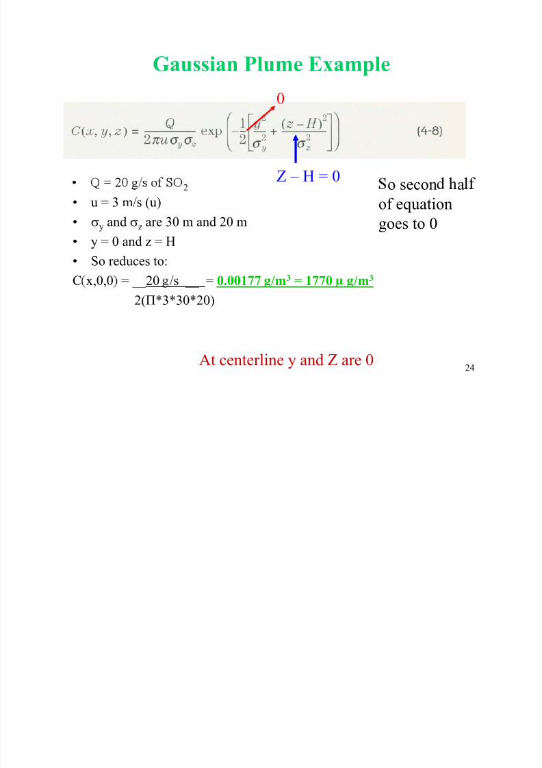
Gaussian Plume Example
0
Z – H = 0 2
• u = 3 m/s (u)
• y and z are 30 m and 20 m
o secon a
of equation
goes to 0• y = 0 and z = H
• So reduces to:
C x,0,0 = 20 /s = 0.00177 /m3 = 1770 /m3 __ __
2(Π*3*30*20)
24
At centerline y and Z are 0

8/22/2019 Dispersion Handout
http://slidepdf.com/reader/full/dispersion-handout 25/72
What are the SO2 concentrations at a point 60 meters to the side and 20
c = ____Q____ exp-1/2[(-y2) + ( (z-H)2)]
2u y z [y2 z
2]
= ___20 g/s___ exp-1/2 [(-60m)2 + (-20m)2] =
2 3*(30)(20) [(30m)2 (202m)]
(0.00177 g/m3) * (exp –2.5) = 0.000145 g/m3 or 145.23 µ g/m3
25
At 20 and 60 meters

8/22/2019 Dispersion Handout
http://slidepdf.com/reader/full/dispersion-handout 26/72
Evaluation of Standard Deviation
• Horizontal and vertical dispersioncoefficients -- are a function
– downwind position x
–
• many experimental measurements –charts
– Correlated y and z to atmospheric stability
26
8/22/2019 Dispersion Handout
http://slidepdf.com/reader/full/dispersion-handout 27/72
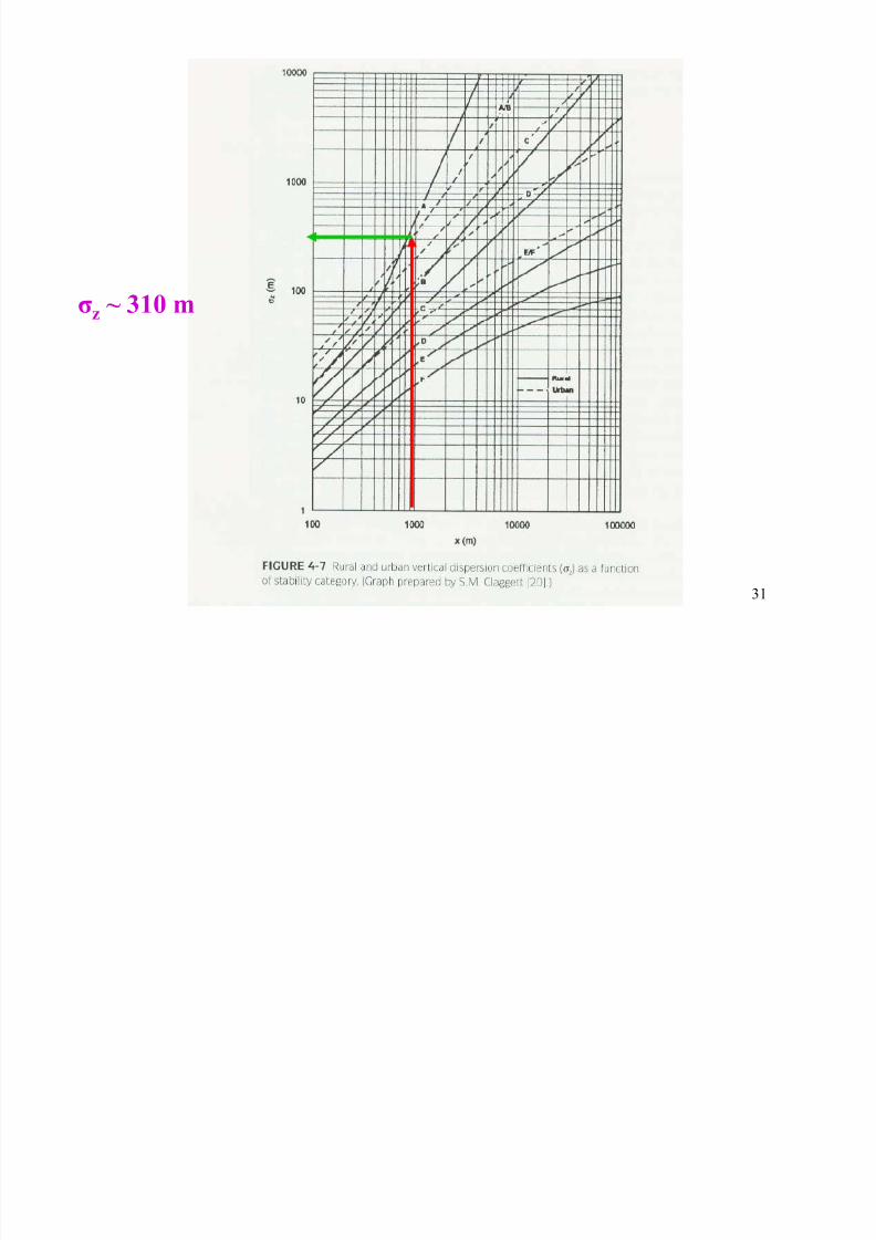
Pasquill-Gifford Curves
• Concentrations correspond to sampling times of approx. 10 minutes
• Regulatory models assume that the concentrations
predicted represent 1-hour averages• Solid curves represent rural values
• Dashed lines represent urban values
• Estimated concentrations represent only the lowestseveral hundred meters of the atmosphere
27
8/22/2019 Dispersion Handout
http://slidepdf.com/reader/full/dispersion-handout 28/72
-• z less certain than y
– Especially for x > 1 km
• For neutral to moderately unstable
atmospheric conditions and distances out to
a few kilometers, concentrations should bewithin a factor of 2 or 3 of actual values
• Tables 3-1: Ke to stabilit classes
28
8/22/2019 Dispersion Handout
http://slidepdf.com/reader/full/dispersion-handout 29/72
Example
For stability class A, what are the values
of y and z at 1 km downstream
(assume urban)
- -
29

8/22/2019 Dispersion Handout
http://slidepdf.com/reader/full/dispersion-handout 30/72
200
σy ~ 220 m
30
8/22/2019 Dispersion Handout
http://slidepdf.com/reader/full/dispersion-handout 31/72
σz ~ 310 m
31

8/22/2019 Dispersion Handout
http://slidepdf.com/reader/full/dispersion-handout 32/72
Example
For sta ty c ass A, w at are t e va ues o
y and z at 1 km downstream
rom a es - an -
= 220 m
z = 310 m
32

8/22/2019 Dispersion Handout
http://slidepdf.com/reader/full/dispersion-handout 33/72
Empirical Equations
• Often difficult to read charts• Curves fit to em irical e uations
y = cxd
= axb
Where
x = ownw n s ance ome ersa, b, c, d = coefficients from Tables 4-1 and 4-2
33
8/22/2019 Dispersion Handout
http://slidepdf.com/reader/full/dispersion-handout 34/72
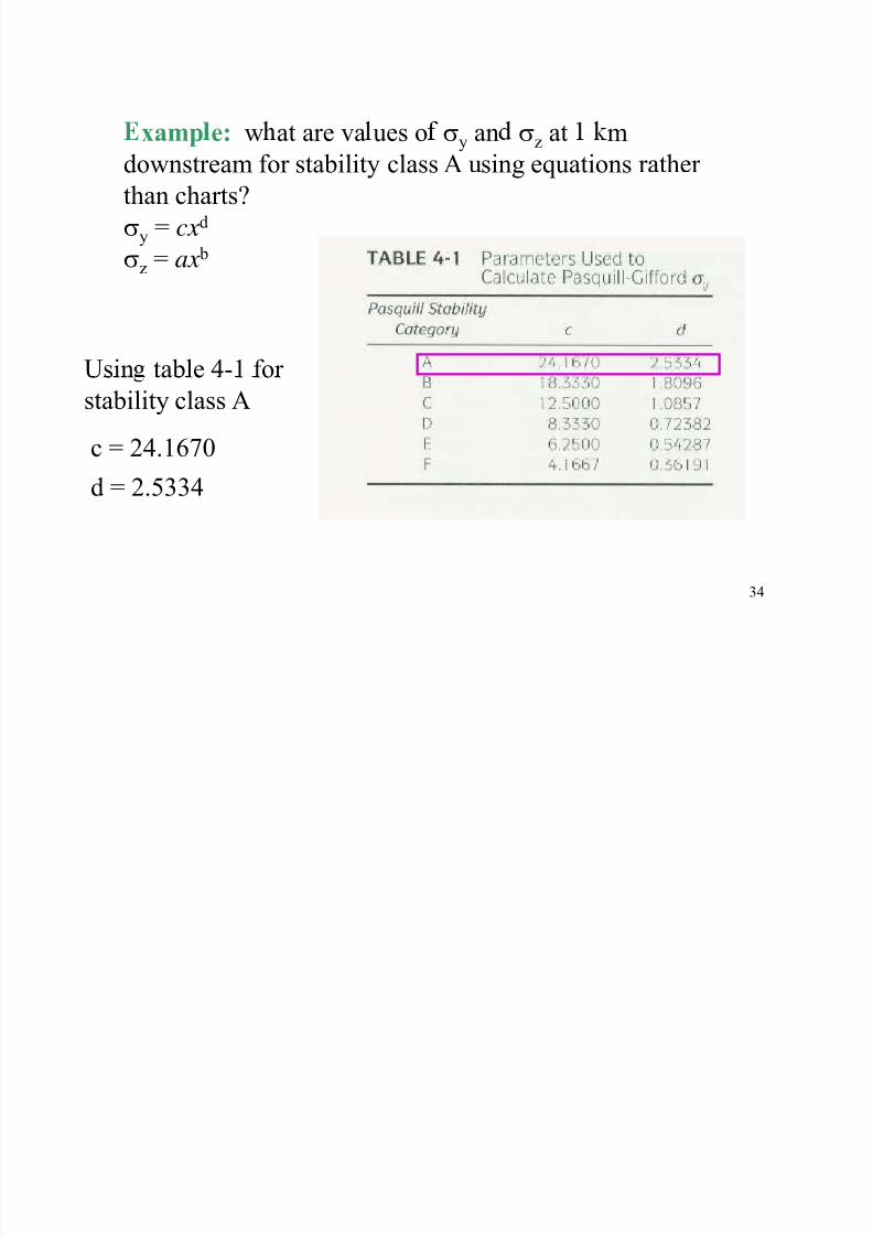
xamp e: w at are va ues o y an z at mdownstream for stability class A using equations rather
than charts?
y
= cxd
z = ax b
Usin table 4-1 for stability class A
c = 24.1670
d = 2.5334
34
8/22/2019 Dispersion Handout
http://slidepdf.com/reader/full/dispersion-handout 35/72
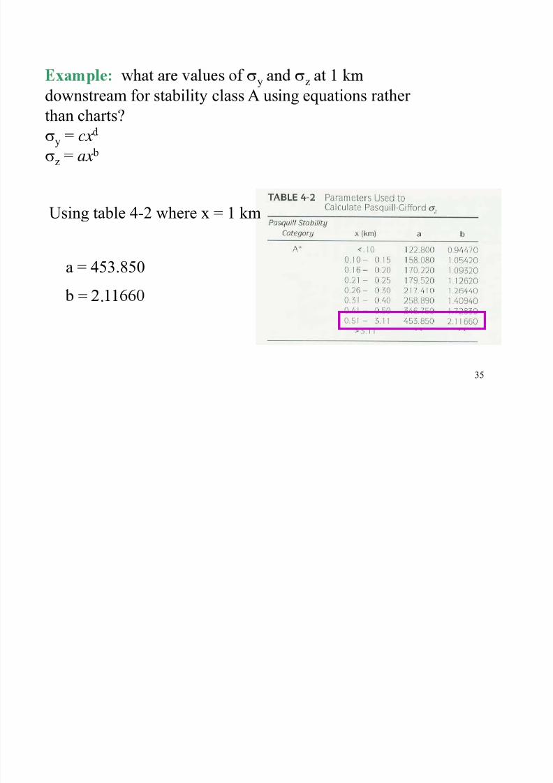
y z downstream for stability class A using equations rather
than charts?
y = cx
z = ax b
Using table 4-2 where x = 1 km
a = 453.850
= .
35
8/22/2019 Dispersion Handout
http://slidepdf.com/reader/full/dispersion-handout 36/72
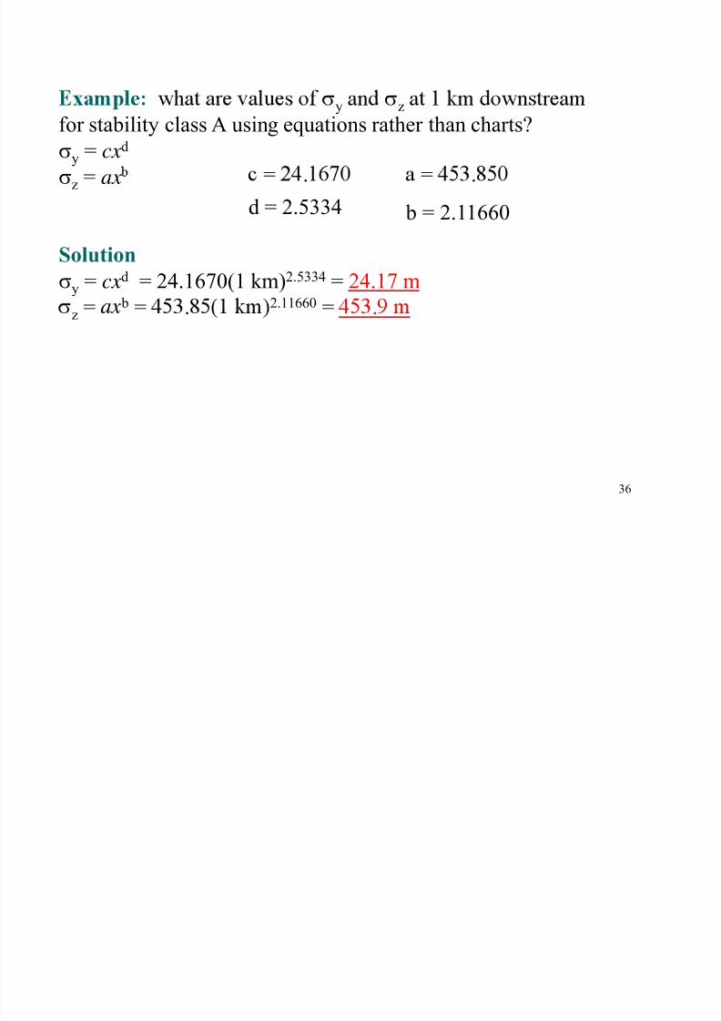
y z for stability class A using equations rather than charts?
y = cxd
z = ax = .
b = 2.11660d = 2.5334
= .
Solution
y = cxd = 24.1670(1 km)2.5334 = 24.17 m
= b = 2.11660 =z . .
36
8/22/2019 Dispersion Handout
http://slidepdf.com/reader/full/dispersion-handout 37/72
Point Source at Elevation H with Reflection
• Previous equation for concentration of lumes a considerable distance above
ground
•
• Pollutants “reflect” back up from ground
37

8/22/2019 Dispersion Handout
http://slidepdf.com/reader/full/dispersion-handout 38/72
Point Source at Elevation H with Reflection
pollutants back into the atmosphere
• e ect on at some stance x s
mathematically equivalent to having am rror mage o t e source at –
• Concentration is equal to contribution of
both plumes at ground level
38

8/22/2019 Dispersion Handout
http://slidepdf.com/reader/full/dispersion-handout 39/72
39

8/22/2019 Dispersion Handout
http://slidepdf.com/reader/full/dispersion-handout 40/72
Point Source at Elevation H with Reflection
Notice this is also equation 4-8 in text,
it is the second e uation 4-8 on the
bottom of page 149
40
8/22/2019 Dispersion Handout
http://slidepdf.com/reader/full/dispersion-handout 41/72
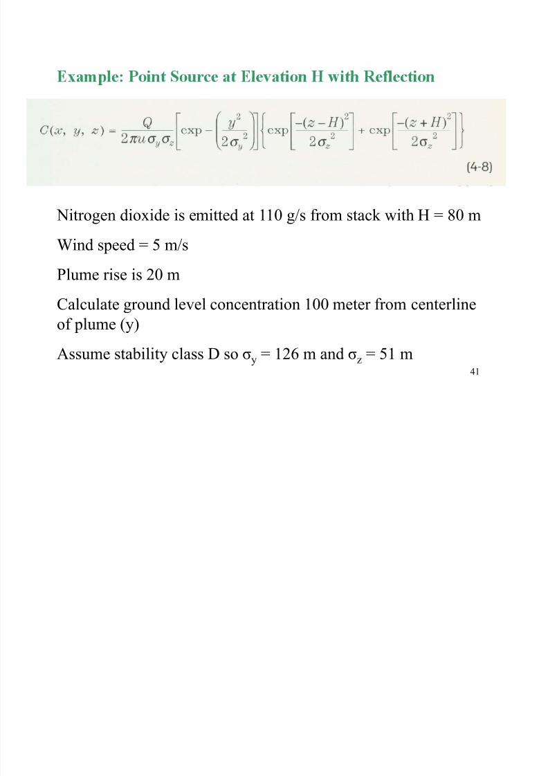
Nitrogen dioxide is emitted at 110 g/s from stack with H = 80 m
Wind speed = 5 m/s
Plume rise is 20 m
Calculate ground level concentration 100 meter from centerlineof plume (y)
41
Assume stability class D so σy = 126 m and σz = 51 m

8/22/2019 Dispersion Handout
http://slidepdf.com/reader/full/dispersion-handout 42/72
Q = 110 g/s H = 80 m u = 5 m/s Δh = 20 m y = 100 m
= =y z
Effective stack height =80 m + 20 m = 100 m
σy = 126 m and σz = 51 m
=
42
_____ ____ .
2Π*5*126*51
8/22/2019 Dispersion Handout
http://slidepdf.com/reader/full/dispersion-handout 43/72
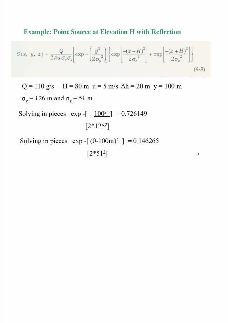
Q = 110 g/s H = 80 m u = 5 m/s Δh = 20 m y = 100 m
= =y z
Solving in pieces exp -[__1002 ] = 0.726149
[2*1252]
- - 2 =
43
.
[2*51
2
]
8/22/2019 Dispersion Handout
http://slidepdf.com/reader/full/dispersion-handout 44/72
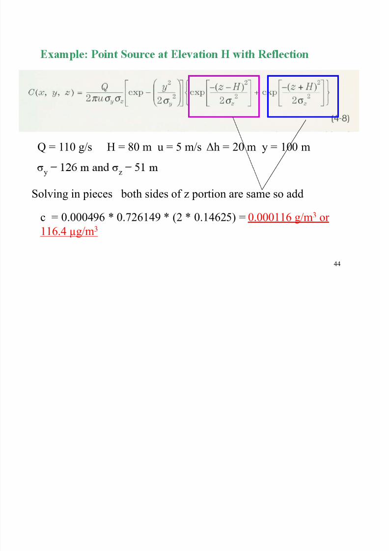
Q = 110 g/s H = 80 m u = 5 m/s Δh = 20 m y = 100 m
= =y z
Solving in pieces both sides of z portion are same so add
c = 0.000496 * 0.726149 * (2 * 0.14625) = 0.000116 g/m3 or 116.4 µg/m3
44

8/22/2019 Dispersion Handout
http://slidepdf.com/reader/full/dispersion-handout 45/72
reflection
• Often want ground level – Peo le ro ert ex osed to ollutants
• Previous eq. gives misleadingly low results
• Pollutants “reflect” back up from ground
45
8/22/2019 Dispersion Handout
http://slidepdf.com/reader/full/dispersion-handout 46/72
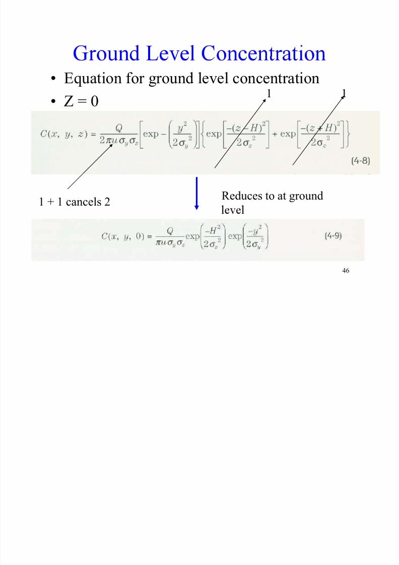
• Equation for ground level concentration
• Z = 0
Reduces to at ground1 + 1 cancels 2
46
G d L l E l
8/22/2019 Dispersion Handout
http://slidepdf.com/reader/full/dispersion-handout 47/72
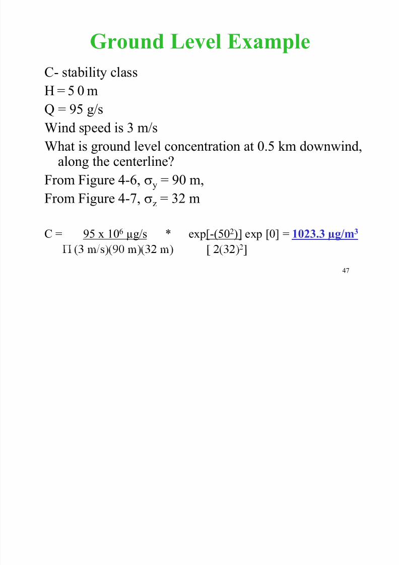
Ground Level Example
C- stability class
H = 5 0 m
Q = 95 g/sWind s eed is 3 m/s
What is ground level concentration at 0.5 km downwind,
along the centerline?From Figure 4-6, y = 90 m,
From Figure 4-7, z = 32 m
C = 95 x 106 µg/s * exp[-(502)] exp [0] = 1023.3 µg/m3
47
8/22/2019 Dispersion Handout
http://slidepdf.com/reader/full/dispersion-handout 48/72
Concentration
• Effect of ground reflection increases groundconcentration
• Does not continue indefinitely
-
(crosswind) and z-direction decreases
48

8/22/2019 Dispersion Handout
http://slidepdf.com/reader/full/dispersion-handout 49/72
Concentration
Values for a, b, c, d are in Table 4-5
49
8/22/2019 Dispersion Handout
http://slidepdf.com/reader/full/dispersion-handout 50/72
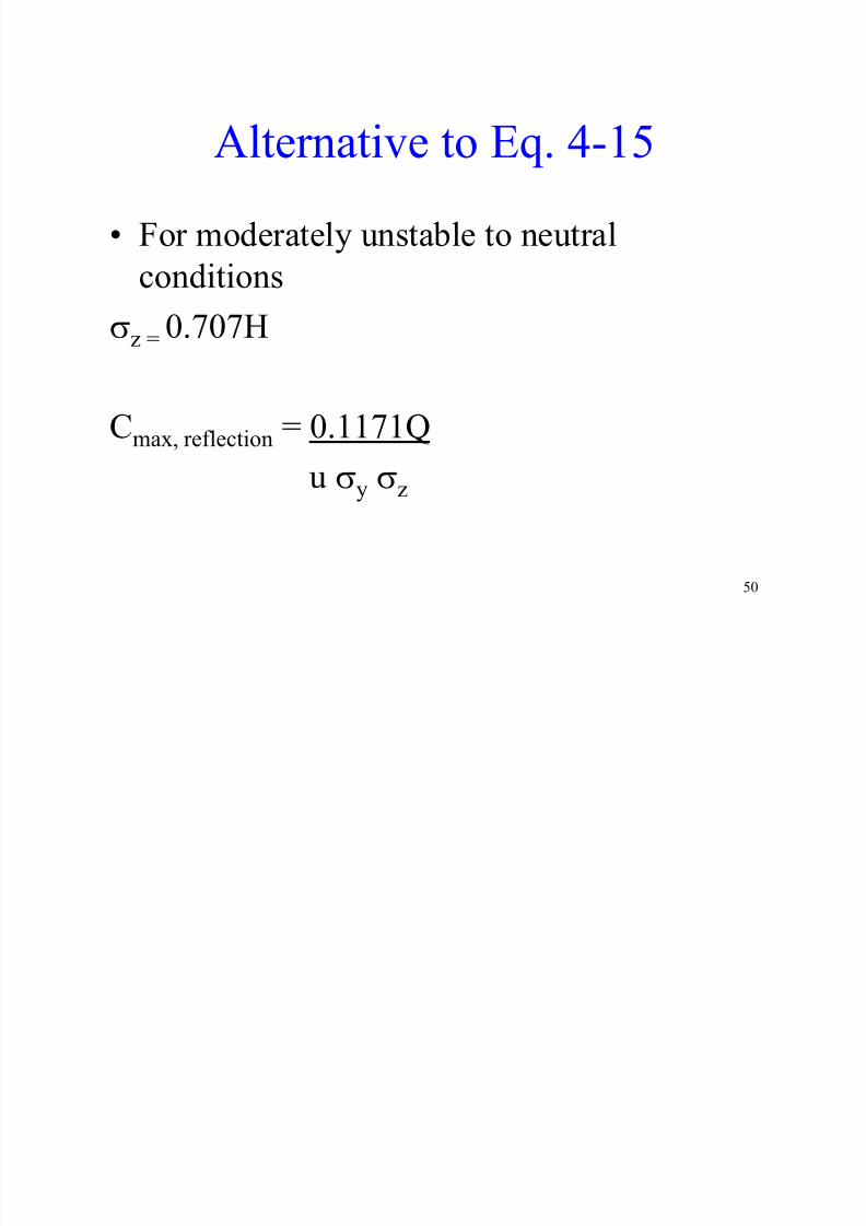
Alternative to Eq. 4-15
• For moderately unstable to neutralconditions
z = 0.707H
Cmax, reflection = 0.1171Q
u y z
50
8/22/2019 Dispersion Handout
http://slidepdf.com/reader/full/dispersion-handout 51/72
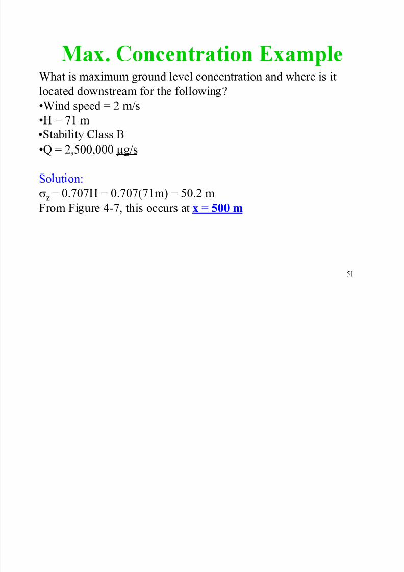
.What is maximum ground level concentration and where is it
located downstream for the followin ?
•Wind speed = 2 m/s
•H = 71 m
•Q = 2,500,000 µg/s
So ut on:
z = 0.707H = 0.707(71m) = 50.2 m
From Fi ure 4-7, this occurs at x = 500 m
51
8/22/2019 Dispersion Handout
http://slidepdf.com/reader/full/dispersion-handout 52/72
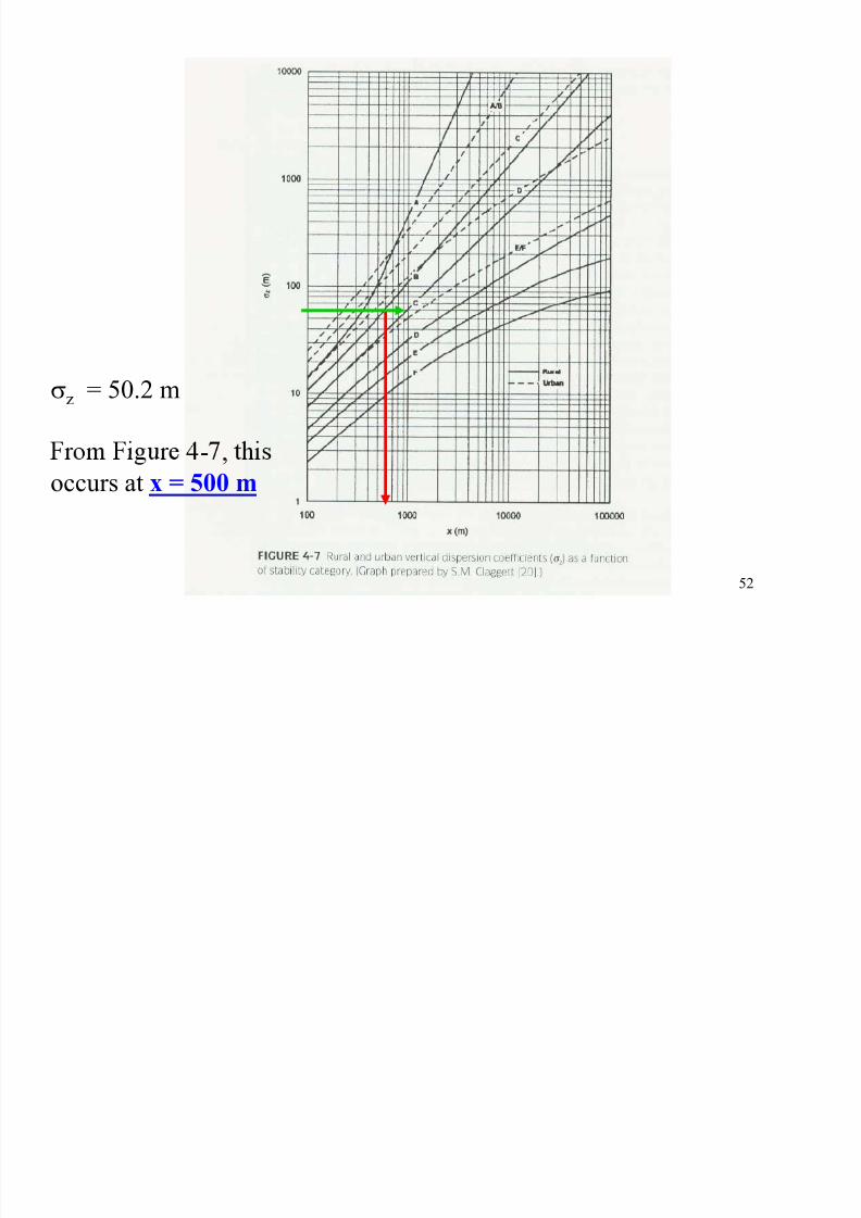
z = 50.2 m
- ,
occurs at x = 500 m
52

8/22/2019 Dispersion Handout
http://slidepdf.com/reader/full/dispersion-handout 53/72
At 500 m, σy =
120 m
53

8/22/2019 Dispersion Handout
http://slidepdf.com/reader/full/dispersion-handout 54/72
.What is maximum ground level concentration and where is it
located downstream for the followin ?
•Wind speed = 2 m/s
•H = 71 m
•Q = 2,500,000 µg/s
So ut on:
z = 0.707H = 0.707(71m) = 50.2 m
From Fi ure 4-7, this occurs at x = 500 m
From Figure 4-6, y = 120 mCmax, reflection = 0.1171Q = 0.1171(2500000) = 24.3 µg/m3
54
u y z (2)(120)(50.2)
8/22/2019 Dispersion Handout
http://slidepdf.com/reader/full/dispersion-handout 55/72
Calculation of Effective Stack Hei ht
• H = hs + Δh•
– Stack characteristics
–
– Physical and chemical nature of effluent
• ar ous equa ons ase on erencharacteristics, pages 162 to 166
55

8/22/2019 Dispersion Handout
http://slidepdf.com/reader/full/dispersion-handout 56/72
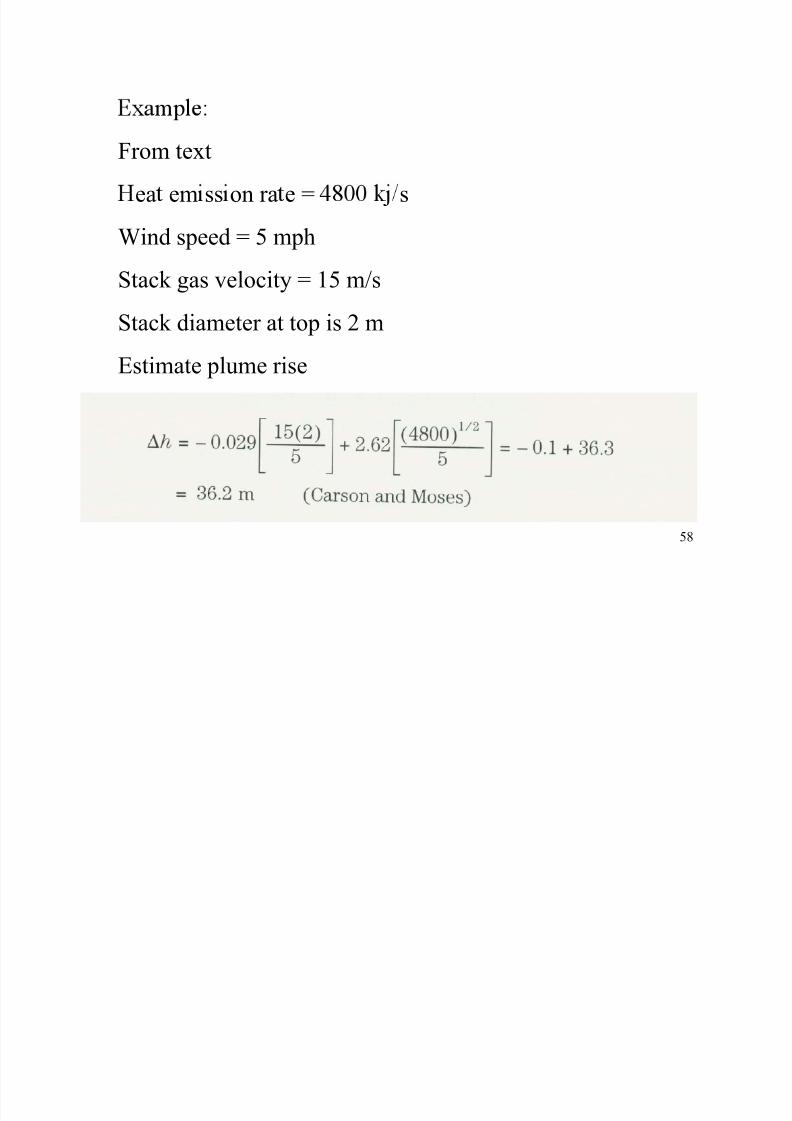
Carson and Moses
• Equation 4-18
Where:
=Vs = stack gas exit velocity (m/s)
d = stack exit diameter meters
us = wind speed at stack exit (m/s)Qh = heat emission rate in kilojoules per second
56
8/22/2019 Dispersion Handout
http://slidepdf.com/reader/full/dispersion-handout 57/72
Other basic equations
• Holland•
57
8/22/2019 Dispersion Handout
http://slidepdf.com/reader/full/dispersion-handout 58/72
From text
ea em ss on ra e = s
Wind speed = 5 mph
Stack gas velocity = 15 m/s
Stack diameter at top is 2 mEstimate plume rise
58
Concentration Estimates for Different

8/22/2019 Dispersion Handout
http://slidepdf.com/reader/full/dispersion-handout 59/72
Concentration Estimates for Different
amp ng mes• Concentrations calculated in previous examples based
-
• Current regulatory applications use this as 1-hour
• For other time periods adjust by:
– 3-hr multiply 1-hr value by 0.9 – 8-hr multiply 1-hr value by 0.7
– 24-hr multiply 1-hr value by 0.4
– annua mu p y - r va ue y . – .
59
Concentration Estimates for Different

8/22/2019 Dispersion Handout
http://slidepdf.com/reader/full/dispersion-handout 60/72
Concentration Estimates for Different
amp ng mes— xamp e• For other time periods adjust by:
– - r mu p y - r va ue y .
– 8-hr multiply 1-hr value by 0.7 – 24-hr multi l 1-hr value b 0.4
– annual multiply 1-hr value by 0.03 – 0.08
Conversion of 1-hr concentration of previous example to an 8-hour average =
c = 36.4 /m3 x 0.7 = 25.5 /m3-
60
8/22/2019 Dispersion Handout
http://slidepdf.com/reader/full/dispersion-handout 61/72
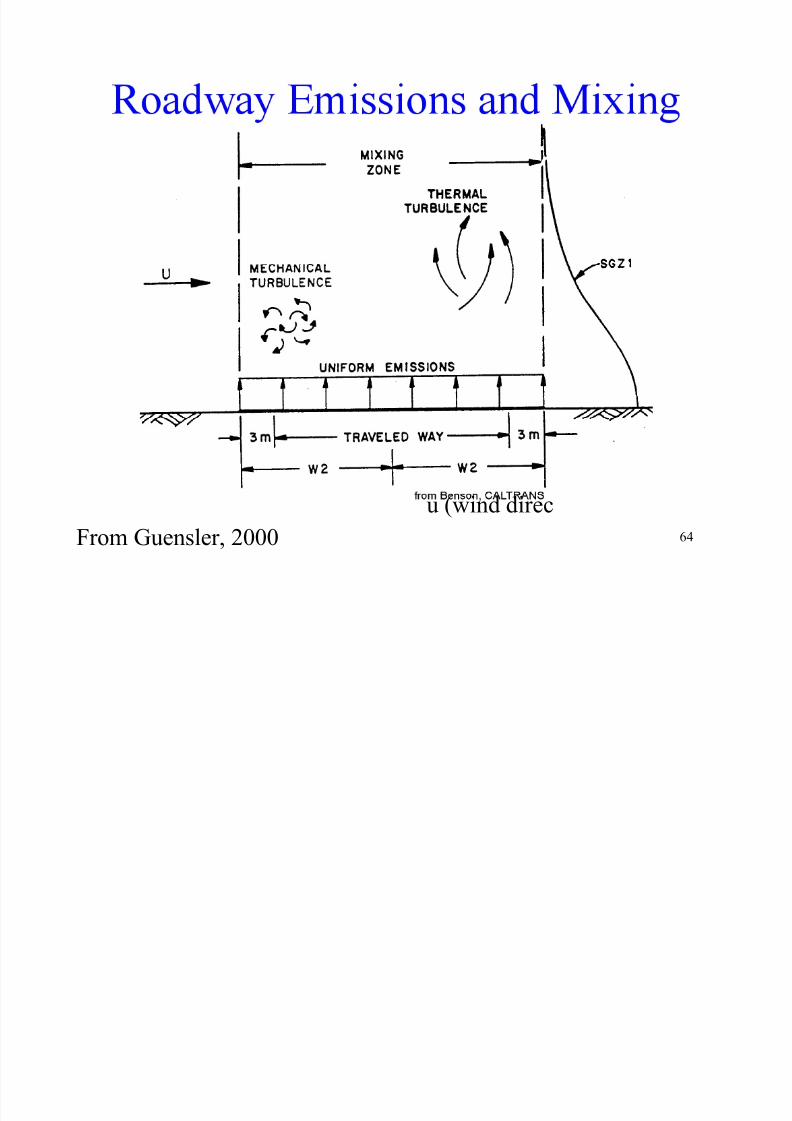
Line Sources
• Imagine that a line source, such as ahi hwa consists of an infinite number of
point sources
•elements, each representing a point source,
summed to predict net concentration
61
8/22/2019 Dispersion Handout
http://slidepdf.com/reader/full/dispersion-handout 62/72
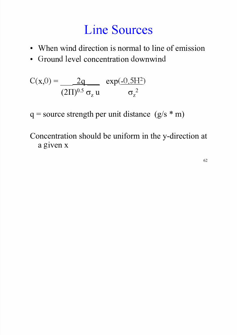
• When wind direction is normal to line of emission
• roun eve concentrat on ownw n
x, = ___ q ___ exp - .
(2Π)0.5 z u z2
q = source strength per unit distance (g/s * m)
Concentration should be uniform in the y-direction ata iven x
62
8/22/2019 Dispersion Handout
http://slidepdf.com/reader/full/dispersion-handout 63/72
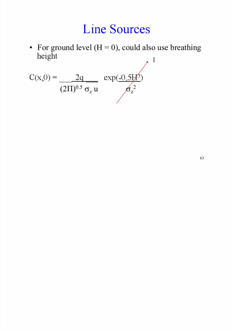
• For ground level (H = 0), could also use breathing
2
1
, ___ ___ - .
(2Π)0.5 z u z2
63
8/22/2019 Dispersion Handout
http://slidepdf.com/reader/full/dispersion-handout 64/72
64From Guensler, 2000
u (wind direc
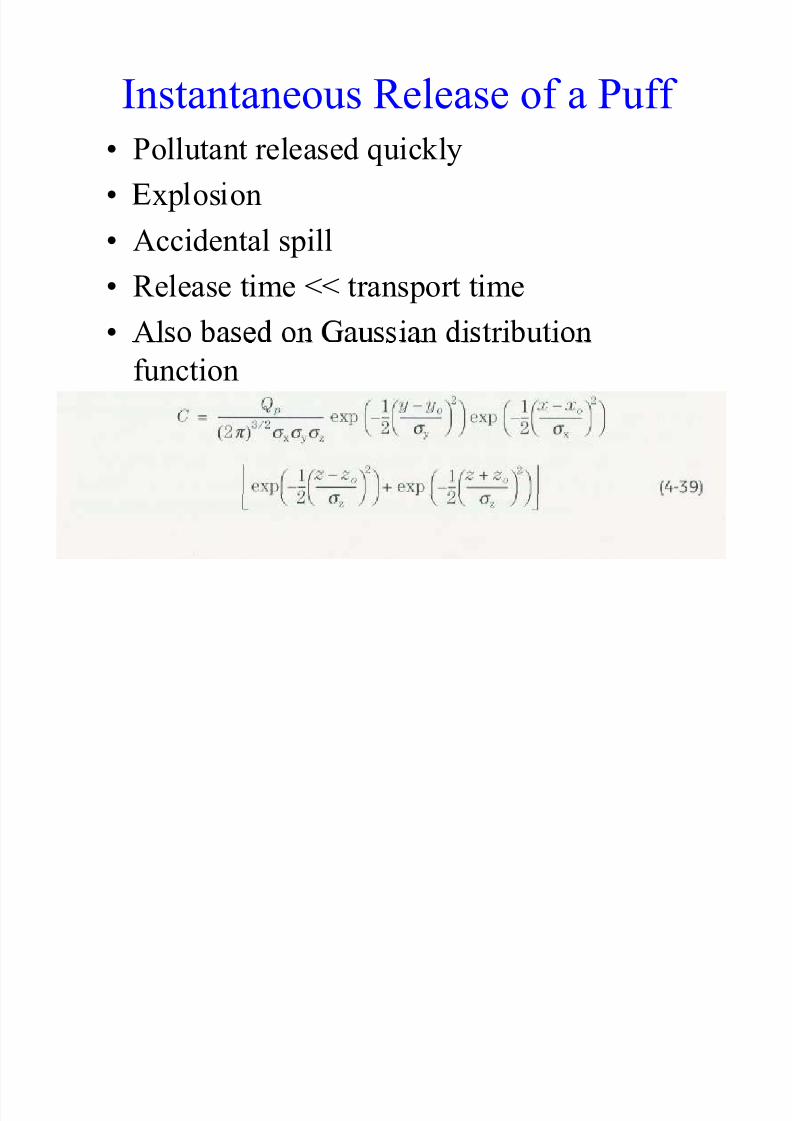
Instantaneous Release of a Puff
8/22/2019 Dispersion Handout
http://slidepdf.com/reader/full/dispersion-handout 65/72
Instantaneous Release of a Puff
• Pollutant released quickly
• xp os on
• Accidental spill
• Release time << transport time
• Al n i n i ri i n function
65

8/22/2019 Dispersion Handout
http://slidepdf.com/reader/full/dispersion-handout 66/72
Instantaneous Release of a Puff • E uation 4-41 to redict maximum round level
concentration
Cmax = _____2Qp____
(2Π)3/2 x
y
z
Receptor downwind would see a gradual increase inconcen ra on un cen er o pu passe an en
concentration would decrease
=
66
x y

8/22/2019 Dispersion Handout
http://slidepdf.com/reader/full/dispersion-handout 67/72
Figure 4-9 and Table 4-7
67

8/22/2019 Dispersion Handout
http://slidepdf.com/reader/full/dispersion-handout 68/72
Figure 4-9 and Table 4-7
68

8/22/2019 Dispersion Handout
http://slidepdf.com/reader/full/dispersion-handout 69/72
Puff Example, .
What exposure will vehicles directly behind the tanker (downwind)receive if x =100 m? Assume very stable conditions.
From Table 4-7,
69

8/22/2019 Dispersion Handout
http://slidepdf.com/reader/full/dispersion-handout 70/72
Figure 4-9 and Table 4-7
70

8/22/2019 Dispersion Handout
http://slidepdf.com/reader/full/dispersion-handout 71/72
Puff Example, .
What exposure will vehicles directly behind the tanker (downwind)receive if x =100 m? Assume very stable conditions.
From Table 4-7, y = 0.02(100m)0.89 = 1.21
rom a e - , z = . m . = .
x = y = 1.21
71

8/22/2019 Dispersion Handout
http://slidepdf.com/reader/full/dispersion-handout 72/72
Puff Example, .
What exposure will vehicles directly behind the tanker (downwind)receive if x =100 m? Assume very stable conditions.
From Table 4-7, y = 0.02(100m)0.89 = 1.21
rom a e - , z = . m . = .
Cmax
= _____2Q p
____ = ____2(400000 g)_____ = 42,181 g/m3
(2Π)3/2 x y z (2Π)3/2(1.21)(1.21)(0.83)
72

![Logic Models Handout 1. Morehouse’s Logic Model [handout] Handout 2](https://cdn.vdocument.in/doc/165x107/56649e685503460f94b6500c/logic-models-handout-1-morehouses-logic-model-handout-handout-2.jpg)


