Applied Probability Trust (18 August 2005)
EOQ ANALYSIS UNDER STOCHASTIC
PRODUCTION AND DEMAND RATES
VIDYADHAR KULKARNI,∗ UNC-Chapel Hill
KEQI YAN,∗∗ UNC-Chapel Hill
Abstract
In this paper we study a type of production-inventory system in which the
production and demand rates are modulated by a background state process
modeled as a finite state Continuous Time Markov Chain (CTMC). When the
production rate exceeds the demand rate, the inventory level increases, and
when the demand rate exceeds the production rate, it decreases. When the
inventory level reaches zero, an order is placed from an external supplier, and
it arrives instantaneously. We model this system as a bivariate Markovian
stochastic process and derive the limiting distribution of the inventory level.
Assuming linear holding costs and fixed ordering costs, we show that the
classical deterministic Economic Order Quantity (EOQ) policy minimizes the
long-run average cost if one replaces the deterministic demand rate by the
expected demand - production rate in steady state. Finally, we extend the
model to allow backlogging.
Keywords: inventory theory, CTMC, uniform distribution, optimal ordering
policy, EOQ
AMS 2000 Subject Classification: Primary 90B05
Secondary 60J25
1. Introduction
In this paper we study a production-inventory model operating in a stochastic
environment that is modulated by a finite state CTMC. A production rate and a
demand rate are associated with each state of the CTMC. The inventory on hand thus
fluctuates according to the state of the CTMC. Once the inventory level drops to 0 a
∗ Postal address: Department of Statistics and Operations Research, University of North Carolina,
Chapel Hill, NC, 27599, USA
1
2 V. Kulkarni and K. Yan
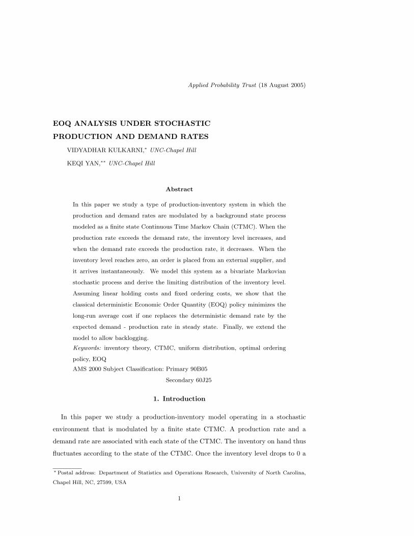
replenishment order of size q is placed. We assume that the lead time is zero, i.e., the
replenishment order is delivered instantaneously, thus the inventory level jumps from
0 to q instantaneously. Figure 1 illustrates a sample path of the inventory level.
Figure 1: A sample path of the inventory level.
This model reflects situations in which the production and demand rates undergo
recurring changes in a stochastic fashion. For instance, the demand rates can change
seasonally; or, in a machine shop the production rate can change according to the
number of working machines, etc. We assume the order size is q regardless of the state
of the CTMC in which the inventory level hits zero. This is an appropriate model
when we can base our inventory replenishment decisions only on the inventory level
and not on the state of the CTMC. This may be because knowledge of the state of the
background CTMC is unavailable, or to simplify the ordering policies. We shall study
the ordering policies based on the state of the CTMC in a subsequent paper.
The objective is to find the replenishment order size q that minimizes the long-run
average cost. The total cost includes costs to hold products in inventory, to purchase
and to produce. There is also a fixed set-up cost every time an order is placed with
an external supplier. To begin with, we assume backlogging is not allowed. (We treat
the backlogging case in Section 6.) Since we assume zero lead time, it is optimal to
place an order only when the inventory reaches zero. In this paper, we establish the
stochastic EOQ theorem that shows the standard deterministic EOQ formula remains
optimal if we replace deterministic demand rate by the expected net demand rate in
steady state.
In the literature, a large variety of inventory models is studied, although many of
them are deterministic [13]. For stochastic models, fluid models are widely used as
one type of approximations [9]. There are several papers concerning fluid models when
EOQ Analysis under Stochastic Production and Demand Rates 3
the production and demand rates depend on the inventory level [1]. As for the cases
when the production and demand rates are determined by the system environmental
state, Berman, Stadje, and Perry recently studied an EOQ model with a two-state
random environment [2]. They consider order sizes that depend on the state of the
environmental state and derived the EOQ policy to optimize the system revenue/cost.
In the general n-state systems, Browne and Zipkin studied a model with continuous
demand driven by a Markov process [3], which can be regarded as a special case of
the model in this paper. Similarly, the clearing processes [11] can be regarded as the
reverse of the inventory level process in a special case when the production rate is
always less than or equal to the demand rate. In that case we show that the inventory
level in steady state is uniformly distributed. However, the stationary distribution of
the content in a clearing system has been proved to be uniform in [4] only under certain
conditions. These conditions are too restrictive and are not satisfied by our model. In
[11] and [12] the authors show that the limiting distribution of the content in a clearing
system is almost never uniform. In this context our result about asymptotically uniform
distribution is even more unexpected.
The rest of this paper is organized as follows. In section 2, we describe the model
mathematically. In Section 3 we derive a system of differential equations for the joint
distribution function of the inventory level and environmental state in steady state and
then solve the equations. We give explicit expressions for two special examples: one
is when the production rate is always less than or equal to the demand rate for every
state. The other is a two-state model and we consider two cases: when the production
rate is less than or equal to the demand rate, or not. In section 4 we compute the
long-run average cost. In section 5, we present the optimal order size q∗ that minimizes
this cost. We show the optimality of a stochastic version of the classical EOQ policy.
Furthermore, in section 6 we extend the results to a more general case that allows
backorders. We show that all the results for the limiting behaviors and expected costs
hold in this new model, and the optimal policy is equivalent to the classical backlogging
EOQ in deterministic models under certain conditions.
4 V. Kulkarni and K. Yan
2. The model
Consider a production-inventory system that is modulated by a stochastic process
{Z(t), t ≥ 0} on state space S = {1, 2, ..., n}. We assume that {Z(t), t ≥ 0} is an
irreducible CTMC on {1, 2, ..., n} with rate matrix Q = [qij ]. When Z(t) is in state i,
the production occurs continuously at rate ri, and there is a demand at rate di. The
net production rate is thus Ri = ri−di. Note that Ri may be negative or positive. Let
X(t) be the inventory level at time t. Then as long as Z(t) = i, {X(t), t ≥ 0} changes
at rate Ri. When X(t) reaches zero we place an order of size q > 0 from an external
supplier who delivers it instantaneously.
Let
π = [π1, π2, · · · , πn] (2.1)
be the limiting distribution of the CTMC, i.e., it is the unique solution to
πQ = 0, π · e = 1,
where e = [1, ..., 1]t is an n-dimensional column vector of ones. The system is stable if
the expected net input raten∑
i=0
πiRi < 0. Let R = diag(R1, ..., Rn). Then the stability
condition can be written in matrix form as follows
πRe < 0. (2.2)
We assume that this stability condition holds for the rest of this paper.
Next we consider costs to operate the system. The total cost consists of three parts:
holding cost, ordering cost, and production cost. We need the following notation to
describe the costs in subsequent sections:
h: cost to hold one item in inventory for one unit of time;
k: fixed set-up cost whenever an order is placed;
p1: cost to purchase one item from the external supplier;
p2: cost to produce one item.
We are interested in computing the optimal order size q∗ that minimizes the long-run
total cost per unit of time. We first need to compute the complementary cumulative
distribution function of the inventory level in steady state. We do this in the next
section.
EOQ Analysis under Stochastic Production and Demand Rates 5
3. Limiting behavior of the inventory level process
In this section we analyze the limiting distribution of the inventory level by a system
of differential equations and solve it with a group of boundary conditions.
3.1. Differential equations
Denote
Gj(t, x) := P{X(t) > x,Z(t) = j}, x ≥ 0, t ≥ 0, j ∈ S.
Assume the stability condition (2.2) thus the following limit exists:
Gj(x) := limt→∞
P{X(t) > x,Z(t) = j}, x ≥ 0, t ≥ 0, j ∈ S.
In this section we show how to compute Gj(x). The following theorem gives the
differential equations satisfied by
G(x) := (G1(x), ..., Gn(x)) .
We use the notation
G′(x) :=(
dG1(x)dx
, ...,dGn(x)
dx
).
Theorem 3.1. The limiting distribution G(x) satisfies
G′(x)R = G(x)Q + β, x ≤ q, (3.1a)
G′(x)R = G(x)Q, x > q, (3.1b)
where the row vector β is given by β := G′(0)R. The boundary conditions are given by
Gj(q+) = Gj(q−), ∀j : Rj 6= 0 (3.2a)
G′j(0) = 0, ∀j : Rj > 0, (3.2b)
G(0)e = 1. (3.2c)
Proof. The differential equations follow from the standard derivation of Chapman
Kolmogorov equations for Markov processes, and hence we omit the details. See [6].
The boundary condition (3.2b) holds because 1/G′j(0) can be seen to be the expected
time between two consecutive visits by the {(X(t), Z(t)), t ≥ 0} process to the state
(0, j). If Rj > 0, this mean time is infinity. Hence G′j(0) = 0 when Rj > 0.
6 V. Kulkarni and K. Yan
The boundary condition Gj(q+) = Gj(q−) for all state j with Rj 6= 0 is obvious
from the fact that there is no probability mass at (q, j) unless Rj = 0. If Rj = 0, it is
easy to show that the probability mass P{X = q, Z = j} satisfies
P{X = q, Z = j}∑k 6=j
qjk =∑
i:Ri<0
G′i(0)Ri.
Thus the boundary condition (3.2a) does not hold for state j if Rj = 0.
3.2. Solution to the differential equations
In this section we derive the solution to the differential equations given in Theorem
3.1. First consider the homogeneous equations G′(x)R = G(x)Q. Let (λ, φ) be an
(eigenvalue, eigenvector) pair that solves
φQ = λφR. (3.3)
Let
m = |{i : Ri 6= 0}|.
Then it is known that there are exactly m pairs (λi, φi), 1 ≤ i ≤ m, that satisfy
Equation (3.3). Assume that they are distinct. Exactly one of the eigenvalues is zero,
and the eigenvector corresponding to this eigenvalue is π, the stationary vector of Q
[7]. Assume that λ1 = 0 and φ1 = π.
We need the following matrix notation
Λ := diag(λ1, λ2, ..., λm), (3.4)
and
Φ :=[φT
1 , φT2 , ..., φT
m
]T. (3.5)
Lemma 3.1. The general solution to the homogeneous equations G′(x)R = G(x)Q
is given by G(x) = ceΛxΦ, where c = (c1, c2, ..., cm) is a constant row vector to be
determined by boundary conditions.
Proof. See [7].
Now take into consideration the non-homogeneous equations G′(x)R = G(x)Q + β.
We have the following theorem.
EOQ Analysis under Stochastic Production and Demand Rates 7
Theorem 3.2. The solution to the differential equations in Theorem 3.1 is given by
G(x) = ceΛxΦ + sxπ + d, if x ≤ q,
G(x) = aeΛxΦ, if x > q,
where the m dimensional row vectors a, c, the n dimensional row vectors d and the
scalar s are the unique solution to the following system of linear equations:
cΛΦR + sπR + dQ = 0, (3.6a)
(aeΛqΦ− ceΛqΦ− sqπ − d)IR 6=0 = 0, (3.6b)
ai = 0, ∀i : λi ≥ 0, (3.6c)m∑
i=0
ciλiφij + sπj = 0, ∀j : Rj > 0, (3.6d)
(cΦ + d)e = 1, (3.6e)
where ai (ci) is the i-th entry of the vector a (c), and IR 6=0 is the modified identity
matrix that has 1 as its j-th diagonal entry if Rj 6= 0, and 0 otherwise.
Proof. According to Lemma 3.1, the homogenous equations (3.1b) have solutions of
form G(x) = ceΛxΦ. It can be shown that the nonhomogeneous equations (3.1a) have
solutions of form
G(x) = ceΛxΦ + sxπ + d (3.7)
if and only if sxπ +d is a particular solution to (3.1a). Thus, using sxπ +d into (3.1a),
we get
sπR = sxπQ + dQ + β
= dQ + β.(3.8)
The last equation holds because πQ = 0.
Sinceβ = G′(0)R
= (cΛΦ + sπ)R,
using β into (3.8) we obtain
sπR = dQ + (cΛΦ + sπ)R,
which can be rearranged to get Equation (3.6a).
8 V. Kulkarni and K. Yan
Suppose when x > q, G(x) has a solution of the form G(x) = aeΛxΦ, where a is
another constant vector.
The boundary condition in Equation (3.2a) reduces to
(aeΛqΦ)IR 6=0 = (ceΛqΦ + sqπ + d)IR 6=0. (3.9)
Rearranging (3.9) we get (3.6b).
Furthermore, boundedness of G(x) as x → ∞ implies Equation (3.6c). Equation
(3.6d) and (3.6e) follow directly from boundary conditions (3.2b) and (3.2c).
The total number of unknown coefficients (a, c, s, d) is 2m + n + 1. Notice that
number of nontrivial equations in (3.6b) is m, and the sum of the number of nontrivial
equations in (3.6c) and (3.6d) is m [7]. Hence we have 2m+n+1 nontrivial equations
to determine a unique solution for the unknown coefficients.
3.3. Examples
Next we study some special cases in which the limiting distributions are interesting.
3.3.1. R ≤ 0 We consider a special case when the production rate never exceeds
the demand rate, and hence the inventory never increases between replenishments.
Without loss of generality assume that X(0) = q. Then it is clear that X(t) ∈ [0, q]
for all t ≥ 0. The next theorem gives the steady-state distribution of X(t).
Theorem 3.3. When R ≤ 0,
G(x) = (1− x
q)π, 0 ≤ x ≤ q. (3.10)
Proof. This is a special case of the model in section 3. The inventory level is always
in [0, q] thus the differential equations reduce to
G′(x)R = G(x)Q + β, (3.11)
where
β = G′(0)R,
with boundary conditions:
G(q) = 0 (3.12a)
G(0)e = 1. (3.12b)
EOQ Analysis under Stochastic Production and Demand Rates 9
It is easy to verify that (3.10) is the solution to the differential equation system (3.11)
with boundary conditions (3.12a) and (3.12b).
Remark 1. Theorem 3.3 implies that in steady state, the inventory level is uniformly
distributed on [0, q], and is independent of Z. This is indeed an unusual and interesting
result. The fact that X is U(0, q) is consistent with the results in [3].
3.3.2. A two-state example Consider a machine shop with only one machine. The
production rate is r when the machine is up, and it fails after an exp(µ) amount of
time. When it is down, there is no production, and it takes exp(λ) amount of time to
fix it. The demand occurs at a constant rate d 6= r no matter whether the machine
is up or down. When the inventory reaches zero, an external supply of amount q is
ordered and arrives instantaneously.
This is a special case with the following parameters:
Q =
−λ λ
µ −µ
, R =
−d 0
0 r − d
.
The matrices Λ (Equation 3.4), Φ (Equation 3.5) and π (Equation 2.1) are given by
Λ =
0 0
0 θ
, Φ =
µ λ
r − d d
,π = (π1, π2)
=(
µλ+µ , λ
λ+µ
),
where
θ =λ(d− r) + dµ
d− r
is the only nonzero eigenvalue.
The stability condition of Equation (2.2) reduces to
λ(r − d)− µd < 0.
Note that θ < 0 if the system is stable. We consider two cases.
Case 1: r > d. In this case, when the machine is up the production rate is greater
than the demand rate. Thus the inventory level hits zero only when the machine is
10 V. Kulkarni and K. Yan
down. We give explicit expressions for the limiting distributions.
Gdown(x) =
1θ π1(eθx − 1
q eθ(x−q)) x > q,
π1(r−d)qθd eθx − π1x + π1
q (1− r−dλ+µ −
rπ2θd ) 0 ≤ x ≤ q,
Gup(x) =
r−dθd π1(eθx − 1
q eθ(x−q)) x > q,
π1qθ eθx − π2x + π1
q (π1π2
+ r−dλ+µ −
rπ1θd ) 0 ≤ x ≤ q.
Case 2: r < d. In this case the inventory level can hit zero when the machine is either
up or down. This is a special case of the model in section 3.3.1. The solution is given
by
Gdown(x) =(
1− 1qx
)µ
λ + µ, 0 ≤ x ≤ q,
Gup(x) =(
1− 1qx
)λ
λ + µ, 0 ≤ x ≤ q.
4. Cost rate calculations
In this section we consider the costs to operate the above system and calculate the
long-run average cost per unit of time.
Let ch(q), co(q) and cp(q) be the steady-state holding, ordering and production cost
rates respectively as functions of the order quantity q. The total cost rate c(q) is hence
given by
c(q) = ch(q) + co(q) + cp(q). (4.1)
The next theorem shows how to compute these cost rates in terms of the limiting
distribution G(x). Let
R̃ := diag(r1, r2, ..., rn),
and
Λ̃ = diag(0,1λ2
, · · · ,1λn
).
Theorem 4.1. The steady-state cost rates are given by
ch(q) = h[(c− a)Λ̃eΛqΦ +
s
2πq2 + (d + c1π)q − cΛ̃Φ
]e,
co(q) = (k + p1q)(cΛΦ + sπ)Re,
cp(q) = p2(cΦ + d)R̃e.
EOQ Analysis under Stochastic Production and Demand Rates 11
Proof. (1) Holding cost rate.
ch(q) =h∑
i
∫ ∞
x=0
Gi(x)dx
=h
[∫ q
x=0
(ceΛxΦ + sπx + d)dx +∫ ∞
x=q
aeΛxΦdx
]e
=h[(c− a)Λ̃eΛqΦ +
s
2πq2 + (d + c1π)q − cΛ̃Φ
]e.
(2) Ordering cost. First consider the number of jumps of the inventory level from 0 to
q during a small time interval (t, t + δ). Notice that when the {Z(t), t ≥ 0} process is
in a state i with negative Ri and X(t) < −Riδ, the number of jumps is 1; otherwise,
it is zero. Thus we have
E( number of jumps in[t, t + δ]) =∑i
P{X(t) ≤ −Riδ, Z(t) = i}
=∑i
(Gi(0)−Gi(−Riδ)).
Hence
limt→∞
limδ→0
1δ E( number of jumps in[t, t + δ]) =
∑i
limδ→0
Gi(0)−Gi(−Riδ)δ
=∑i
RiG′i(0)
= G′(0)Re.
Thus the ordering cost rate is
co(q) = (k + p1q) limt→∞
limδ→0
1δ E( number of jumps in[t, t + δ])
= (k + p1q)G′(0)Re
= (k + p1q)(cΛΦ + sπ)Re.
(3) Production cost rate. In steady state, the probability that the environmental
process is in state i is given by Gi(0). The production cost rate is p2ri when the
environmental process is in state i. Thus the production cost rate is given by
cp(q) =∑i∈S
p2riGi(0)
= p2G(0)R̃e
= p2(cΦ + d)R̃e.
5. Optimal order size
In this section, we demonstrate the primary result of this paper. We use sample
path method to show that the total cost rate c(q) is a convex function of q and that the
12 V. Kulkarni and K. Yan
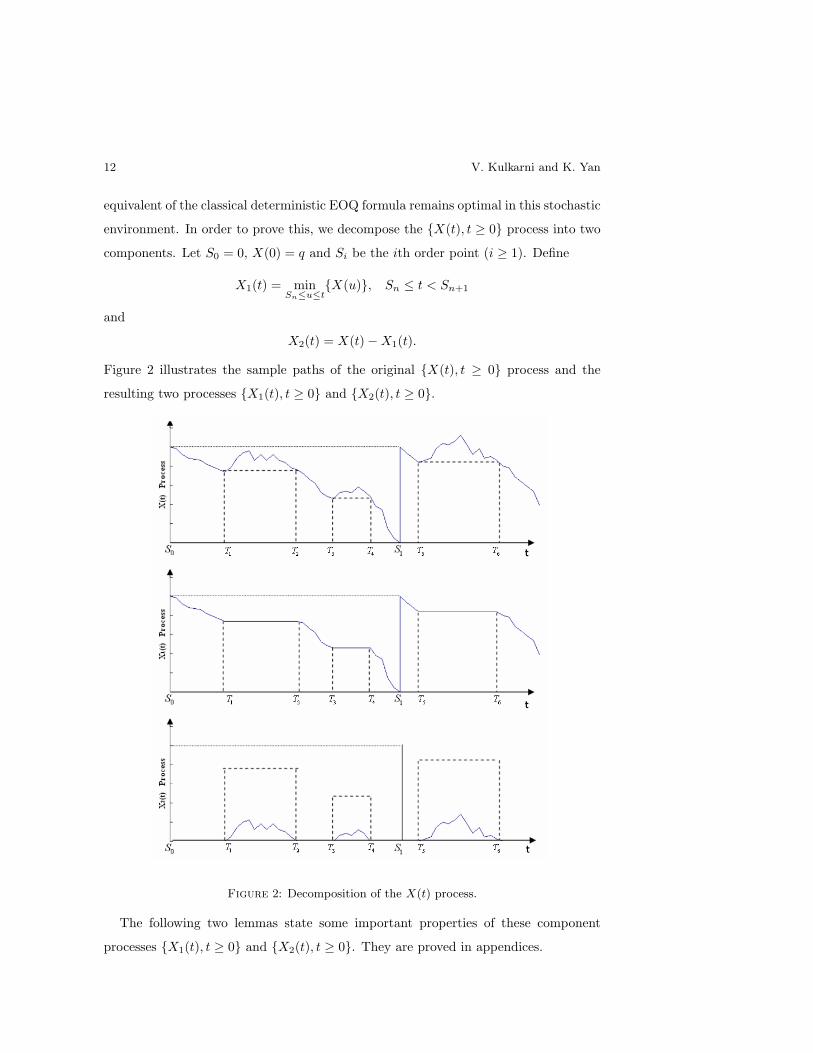
equivalent of the classical deterministic EOQ formula remains optimal in this stochastic
environment. In order to prove this, we decompose the {X(t), t ≥ 0} process into two
components. Let S0 = 0, X(0) = q and Si be the ith order point (i ≥ 1). Define
X1(t) = minSn≤u≤t
{X(u)}, Sn ≤ t < Sn+1
and
X2(t) = X(t)−X1(t).
Figure 2 illustrates the sample paths of the original {X(t), t ≥ 0} process and the
resulting two processes {X1(t), t ≥ 0} and {X2(t), t ≥ 0}.
Figure 2: Decomposition of the X(t) process.
The following two lemmas state some important properties of these component
processes {X1(t), t ≥ 0} and {X2(t), t ≥ 0}. They are proved in appendices.
EOQ Analysis under Stochastic Production and Demand Rates 13
Lemma 5.1. The process {X2(t), t ≥ 0} is independent of q.
Lemma 5.2. The limiting distribution of the process {X1(t), t ≥ 0} is uniform over
[0, q].
Now with these two lammas, we are ready to give the main result of this section.
Theorem 5.1. Let ∆ be the expected net demand rate (i.e., demand rate -production
rate) in steady state, given by
∆ = −∑
i
πiRi. (5.1)
Suppose ∆ > 0. Then the optimal order size q∗ that minimizes the total cost rate c(q)
is given by
q∗ =
√2k∆h
. (5.2)
Proof. From Equation 4.1 the total cost rate is given by
c(q) = ch(q) + co(q) + cp(q)
= hE(X) +k + p1q
E(Si − Si−1)+ cp(q).
First we calculate ch(q).
ch(q) = hE(X)
= h(E(X1) + E(X2)).
According to Lemma 5.2, {X1(t), t ≥ 0} is uniformly distributed on [0, q] in steady
state. Thus E(X1) = q2 . Also, according to Lemma 5.1, we know that {X2(t), t ≥ 0} is
independent of q. Since we have assumed the stability of {X(t), t ≥ 0}, it is clear that
{X2(t), t ≥ 0} has a limiting distribution and it is independent of q. Hence E(X2) is
independent of q.
Next we calculate co(q). From the results on renewal reward processes we get
co(q) =k + p1q
Ei(Si − Si−1).
In steady state, the average net demand during a cycle time (Si, Si−1) has to be equal
to the amount of the external supply. Hence we have
Ei(Si − Si−1)∆ = q.
14 V. Kulkarni and K. Yan
Thus
co(q) =(k + p1q)∆
q
=k∆q
+ p1∆.
Since cp(q) = pi
∑πiri, it is independent of q.
Thus the total cost rate is
c(q) =hq
2+
k∆q
+ C,
where C = hE(X2)+p1∆+cp(q) is independent of q. Clearly, C(q) is a convex function
of q, and it is minimized at q∗ given by 5.2.
Remark 2. The optimal order quantity q∗ of Equation (5.2) is the classical EOQ
formula with the deterministic demand rate replaced by the steady-state expected net
demand rate.
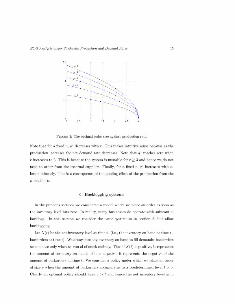
A machine shop example. Consider a machine shop that has n independent and
identical machines, each behaving as described in section 3.3.2. Each machine has its
own repair person. Let Z(t) be the number of working machines at time t. Thus the
CTMC {Z(t), t ≥ 0} has n+1 states, i.e., S = {0, 1, ..., n}. Suppose the demand rate is
directly proportional to the number of machines. Thus we have di = n and ri = i ·r for
all i ∈ S, where r is the production rate of one working machine. Next we investigate
the effect of the production rate increases on the optimal order size q∗. Consider a
system with λ = 1, µ = 2, h = 10, k = 2, p1 = 8 and p2 = 5. We plot the optimal
values of q∗ in Figure 3 for 1 ≤ n ≤ 5 and r varying in (0, 3).
EOQ Analysis under Stochastic Production and Demand Rates 15
Figure 3: The optimal order size against production rate.
Note that for a fixed n, q∗ decreases with r. This makes intuitive sense because as the
production increases the net demand rate decreases. Note that q∗ reaches zero when
r increases to 3. This is because the system is unstable for r ≥ 3 and hence we do not
need to order from the external supplier. Finally, for a fixed r, q∗ increases with n,
but sublinearly. This is a consequence of the pooling effect of the production from the
n machines.
6. Backlogging systems
In the previous sections we considered a model where we place an order as soon as
the inventory level hits zero. In reality, many businesses do operate with substantial
backlogs. In this section we consider the same system as in section 2, but allow
backlogging.
Let X(t) be the net inventory level at time t. (i.e., the inventory on hand at time t -
backorders at time t). We always use any inventory on hand to fill demands; backorders
accumulate only when we run of of stock entirely. Thus if X(t) is positive, it represents
the amount of inventory on hand. If it is negative, it represents the negative of the
amount of backorders at time t. We consider a policy under which we place an order
of size q when the amount of backorders accumulates to a predetermined level l > 0.
Clearly an optimal policy should have q > l and hence the net inventory level is in
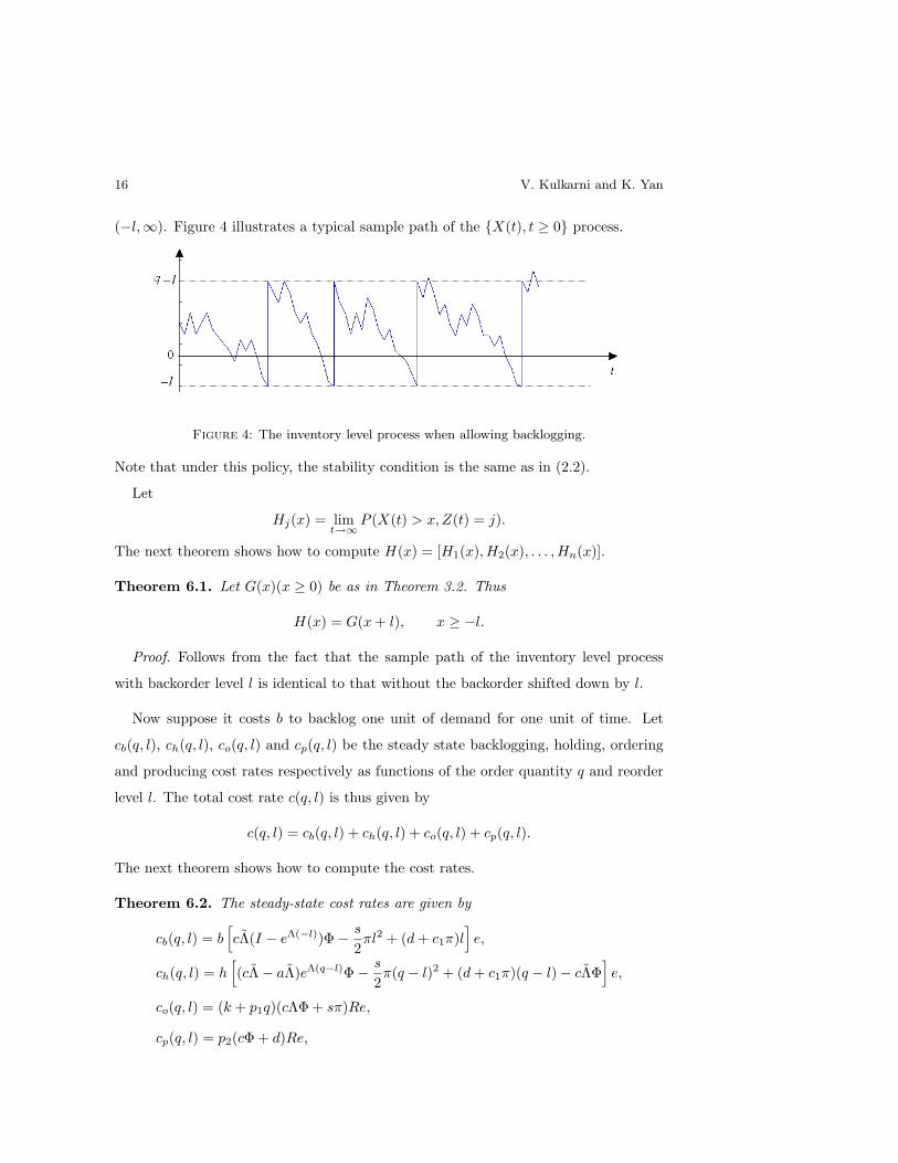
16 V. Kulkarni and K. Yan
(−l,∞). Figure 4 illustrates a typical sample path of the {X(t), t ≥ 0} process.
Figure 4: The inventory level process when allowing backlogging.
Note that under this policy, the stability condition is the same as in (2.2).
Let
Hj(x) = limt→∞
P (X(t) > x,Z(t) = j).
The next theorem shows how to compute H(x) = [H1(x),H2(x), . . . ,Hn(x)].
Theorem 6.1. Let G(x)(x ≥ 0) be as in Theorem 3.2. Thus
H(x) = G(x + l), x ≥ −l.
Proof. Follows from the fact that the sample path of the inventory level process
with backorder level l is identical to that without the backorder shifted down by l.
Now suppose it costs b to backlog one unit of demand for one unit of time. Let
cb(q, l), ch(q, l), co(q, l) and cp(q, l) be the steady state backlogging, holding, ordering
and producing cost rates respectively as functions of the order quantity q and reorder
level l. The total cost rate c(q, l) is thus given by
c(q, l) = cb(q, l) + ch(q, l) + co(q, l) + cp(q, l).
The next theorem shows how to compute the cost rates.
Theorem 6.2. The steady-state cost rates are given by
cb(q, l) = b[cΛ̃(I − eΛ(−l))Φ− s
2πl2 + (d + c1π)l
]e,
ch(q, l) = h[(cΛ̃− aΛ̃)eΛ(q−l)Φ− s
2π(q − l)2 + (d + c1π)(q − l)− cΛ̃Φ
]e,
co(q, l) = (k + p1q)(cΛΦ + sπ)Re,
cp(q, l) = p2(cΦ + d)Re,
EOQ Analysis under Stochastic Production and Demand Rates 17
where a, c, s and d are the coefficients in the expression of H(x) corresponding to
Theorem 3.2.
Proof. Follow the same steps in the proof of Theorem 4.1.
The next theorem gives the stochastic version of the EOQ formula with backloggings.
Theorem 6.3. Let ∆ be as in Equation (5.1), ∆ > 0. Then the optimal order size q∗
and reorder position l∗ are given by
q∗ =
√2k(b + h)∆
hb(6.1)
l∗ =(
h
b + h
)q∗. (6.2)
Proof. Follow the same analysis as in Theorem 5.1.
In particular, when R ≤ 0, {X(t), t ≥ 0} has uniform distribution on (−l, q − l) in
steady state, and is independent of Z, thus
H(x) =(
q − l − x
q
)π, −l ≤ x ≤ q − l,
and the long-run average cost is
c(q, l) =[(
(b + h)l2
2q+
hq
2− hl
)π − k
qπR− p1πR + p2πR̃
]e.
This is consistent with the results in deterministic models [13].
7. Conclusion and future work
We have studied a type of inventory models with or without backlogging having
production and demand rates modulated by a background stochastic process. External
replenishment orders are placed at appropriate times and arrive instantaneously. In
this paper we have modeled this system as a bivariate Markovian stochastic process
and derived the limiting distribution of the inventory level. We have established a
stochastic EOQ theorem that shows the optimality of the classical EOQ policy in this
stochastic environment.
We can study three extensions of this system. In the current analysis, the order size
is not allowed to depend on the state of the CTMC when the inventory level hits zero.
18 V. Kulkarni and K. Yan
Clearly, if that information is available, it would lower the costs if the order size can
be made dependent on that information. Berman, Stadje, and Perry have studied such
a two state system [2]. However, more work on deriving the optimal scenario in more
general systems is needed.
Secondly, in this paper we have assumed zero lead times. This assumption is
reasonable when lead times are short enough to be neglected. It would be interesting
to study this system with nonzero lead times. We feel that iid exponential lead times
may lead to tractable analysis.
Clearly, the results of this paper remain valid if the background process is a semi-
Markov process with Phase-type distributions [10]. This can be shown by constructing
an appropriate larger CTMC. Since Phase-type distributions are dense in the set of all
continuous distributions on [0,∞), it follows that the results hold for a semi-Markov
background process with continuous sojourn times. We believe that the results hold for
more general semi-Markov processes as long as the sample paths of the {X(t), t ≥ 0}
process are not periodic with probability one. Rigorous proof of this remains to be
shown.
Appendix A. Proof of lemma 5.1
Proof. Let S+ and S− be two subsets of S defined as S+ = {i ∈ S : Ri ≥ 0}, and
S− = {i ∈ S : Ri < 0}. Assume that Z(0) ∈ S− and define
T1 = min{t ≥ 0 : Z(t) ∈ S+}.
Regardless of the value of q, X(t) always decreases over (0, T1), except for possible
jumps of size q when it hits zero. Thus X2(t) is zero over (0, T1). T1 is independent of
q and hence {X2(t), t ∈ [0, T1)} is independent of q.
Now define
T2 = min{t > T1 : X(t) = X(T1)}.
Note that T2 is also independent of q, X2(T1) = X2(T2) = 0 and X2(t) > 0 for
t ∈ (T1, T2). The sample path of {X(t), t ∈ (T1, T2)} is independent of q, since X(t)
never reaches 0 for any t ∈ (T1, T2). Thus the sample path of {X2(t), t ∈ (T1, T2)} is
independent of q.
EOQ Analysis under Stochastic Production and Demand Rates 19
Define
T2n+1 = min{t ≥ T2n : Z(t) ∈ S+},
and
T2n+2 = min{t ≥ T2n+1 : X(t) = X(T2n+1)}.
Since {X2(t), t ≥ 0} goes through these two cycles alternately over (T2n, T2n+1) and
(T2n+1, T2n+2) independently, it is clear that {X2(t), t ≥ 0} is independent of q.
Appendix B. Proof of lemma 5.2
Proof. First note that the sample paths of {X1(t), t ≥ 0} have right derivative
everywhere. Define I(t) = 0 if the right derivative of X1(t) is strictly negative at t,
and I(t) = 1 if the right derivative of X1(t) is zero at t. Now
limt→∞
P (X1(t) ≤ x)
= limt→∞
P (X1(t) ≤ x)|I(t) = 0)P (I(t) = 0) + limt→∞
P (X1(t) ≤ x)|I(t) = 1)P (I(t) = 1).
(B.1)
Next we will show that
limt→∞
P (X1(t) ≤ x|I(t) = ζ) = x/q, ζ ∈ {0, 1}. (B.2)
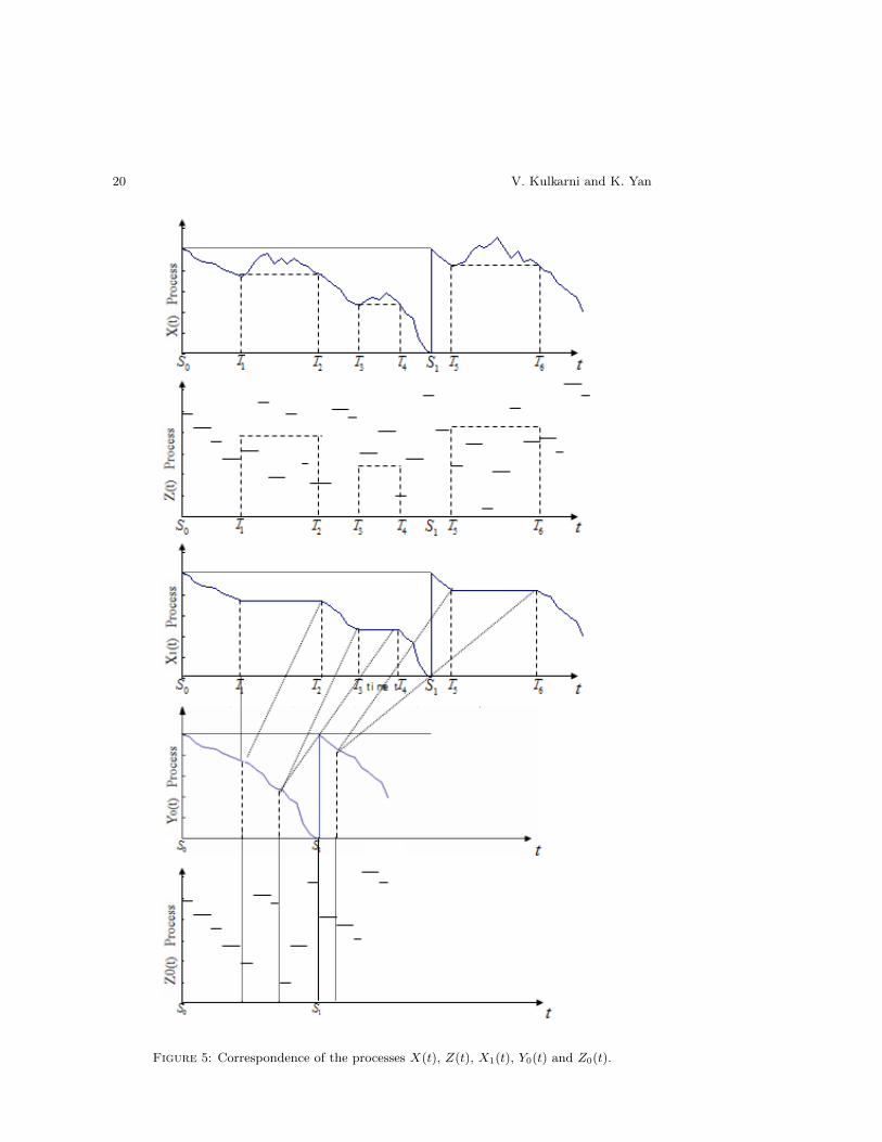
First we construct two new processes {Y0(t), t ≥ 0} and {Z0(t), t ≥ 0} by eliminating
the segments of the sample paths of {X1(t), t ≥ 0} and {Z(t), t ≥ 0} over the time
intervals (T2n+1, T2n+2] for all n ≥ 0. The sample paths of the {Y0(t), t ≥ 0} and
{Z0(t), t ≥ 0} processes corresponding to the sample paths of {X1(t), t ≥ 0} and
{Z(t), t ≥ 0} are shown in Figure 5. From Figure 5 we can see that {Y0, t ≥ 0} can be
thought of as a fluid model modulated by the stochastic process {Z0(t), t ≥ 0} with
state space S−. It can be seen that {Z0(t), t ≥ 0} is a CTMC with generator matrix
Q̂ = [q̂ij ], (i, j ∈ S−) given by
q̂ij = qij +∑
k∈S+
qikηkj , i, j ∈ S−,
where
ηkj = P (Z(T2n+2) = j|Z(T2n+1) = k), k ∈ S+, j ∈ S−.
20 V. Kulkarni and K. Yan
Figure 5: Correspondence of the processes X(t), Z(t), X1(t), Y0(t) and Z0(t).
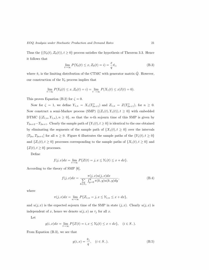
EOQ Analysis under Stochastic Production and Demand Rates 21
Thus the {(Y0(t), Z0(t)), t ≥ 0} process satisfies the hypothesis of Theorem 3.3. Hence
it follows that
limt→∞
P (Y0(t) ≤ x,Z0(t) = i) =x
qπ̂i, (B.3)
where π̂i is the limiting distribution of the CTMC with generator matrix Q̂. However,
our construction of the Y0 process implies that
limt→∞
P (Y0(t) ≤ x,Z0(t) = i) = limt →∞
P (X1(t) ≤ x|I(t) = 0).
This proves Equation (B.2) for ζ = 0.
Now for ζ = 1, we define Y1,n = X1(T+2n+1) and Z1,n = Z(T+
2n+1), for n ≥ 0.
Now construct a semi-Markov process (SMP) {(Z1(t), Y1(t)), t ≥ 0} with embedded
DTMC {(Z1,n, Y1,n), n ≥ 0}, so that the n-th sojourn time of this SMP is given by
T2n+2−T2n+1. Clearly the sample path of {Y1(t), t ≥ 0} is identical to the one obtained
by eliminating the segments of the sample path of {X1(t), t ≥ 0} over the intervals
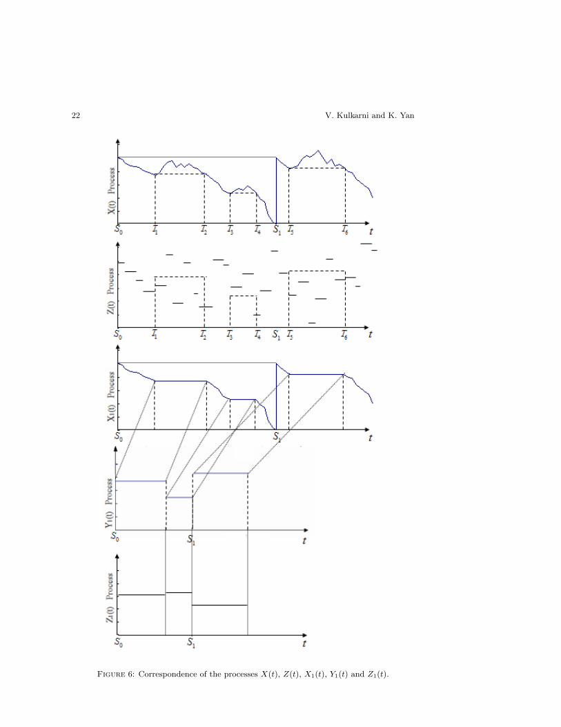
(T2n, T2n+1] for all n ≥ 0. Figure 6 illustrates the sample paths of the {Y1(t), t ≥ 0}
and {Z1(t), t ≥ 0} processes corresponding to the sample paths of {X1(t), t ≥ 0} and
{Z(t), t ≥ 0} processes.
Define
f(j, x)dx = limt→∞
P{Z(t) = j, x ≤ Y1(t) ≤ x + dx}.
According to the theory of SMP [6],
f(j, x)dx =π(j, x)u(j, x)dx∑
k∈S+
∫ q
y=0π(k, y)u(k, y)dy
, (B.4)
where
π(j, x)dx = limn→∞
P{Z1,n = j, x ≤ Y1,n ≤ x + dx},
and u(j, x) is the expected sojourn time of the SMP in state (j, x). Clearly u(j, x) is
independent of x, hence we denote u(j, x) as τj for all x.
Let
g(i, x)dx = limt→∞
P{Z(t) = i, x ≤ Y0(t) ≤ x + dx}, (i ∈ S−).
From Equation (B.3), we see that
g(i, x) =π̂i
q, (i ∈ S−). (B.5)
22 V. Kulkarni and K. Yan
Figure 6: Correspondence of the processes X(t), Z(t), X1(t), Y1(t) and Z1(t).
EOQ Analysis under Stochastic Production and Demand Rates 23
Hence using Equation (B.5),
π(j, x) =∑i∈S−
g(i, x)qij =1q
∑i∈S−
π̂iqij . (B.6)
Substituting Equation (B.6) into (B.4), we have
f(j, x) =
1q
∑i∈S−
π̂iqijτj
∑k∈S+
q∫y=0
1q
∑i∈S−
π̂iqikτkdy
=1q·
∑i∈S−
π̂iqijτj∑k∈S+
∑i∈S−
π̂iqikτk.
Thus the limiting probability density function of {Y1(t), t ≥ 0} process is given by
f(x) =∑
j∈S+
f(j, x) (B.7)
=1q·
∑j∈S+
∑i∈S−
π̂q̂ijτj∑k∈S+
∑i∈S−
π̂q̂ikτk(B.8)
=1q. (B.9)
Equation (B.9) indicates the limiting distribution of {Y1(t), t ≥ 0} is uniform over
[0, q]. This proves Equation (B.2) for j = 1. Hence from (B.1)
limt→∞
P (X1(t) ≤ x) =x
q.
This proves Lemma 5.2.
References
[1] Berman, O. and Perry, D. (2004). An EOQ model with state dependent demand rate. Eur.
J. Operat. Res. In Press.
[2] Berman, O., Stadje, W. and Perry, D. (2005). A Fluid EOQ Model with a Two-State Random
Environment.
[3] Browne, S. and Zipkin, P. (1991). Inventory Models with Continuous Stochastic Demands.
Ann. Appl. Prob. 1, 419–435.
[4] El-Taha, M. (2002). A Sample-Path Condition for the Asymptotic Uniform Distribution of
Clearing Processes. Optimization. 51, 965–975.
24 V. Kulkarni and K. Yan
[5] Kella, O. and Whitt, W. (1992). A storage model with a two state random environment.
Operat. Res. 40, 257–262.
[6] Kulkarni, V. G. (1995). Modeling and Analysis of Stochastic Systems. Chapman and Hall,
London.
[7] Kulkarni, V. G. (1997). Fluid models for single buffer systems, in: J. H. Dshalalow
(Ed.), Frontiers in Queueing, Models and Applications in Science and Engineering, Ed. J.H.
Dshalalow, CRC Press, Boca Raton, FL, 321–338.
[8] Kulkarni, V. G. and Tzenova, E. (2002). Mean first passage times in fluid queues. Operat.
Res. Lett. 30, 308–318.
[9] Mitra, D. (1988). Stochastic theory of a fluid model of producers and consumers coupled by a
buffer. Adv. Appl. Prob. 20, 646–676.
[10] Neuts, M. F. (1981). Matrix Geometric Solutions in Stochastic Models. Johns Hopkins
University Press, Baltimore, MD.
[11] Serfozo, R. and Stidham, S. (1978). Semi-stationary clearing processes. Stoch. Proc. Appl. 6,
165–178.
[12] Whitt, W. (1981). The stationary distribution of a stochastic clearing process. Operat. Res. 29,
294–308.
[13] Zipkin, P. (2000). Foundations of Inventory Management. McGraw-Hill, Boston.


