
EXPORT PRODUCTION DEPTH OF EMILI ANI A HUXLEY/IN THE GULF OF
CALIFORNIA: AN EVALUATION OF THE ALKENONE UK'37 PALEOSST-PROXY
A THESIS SUBMITTED TO THE GRADUATE DIVISION OF THE UNIVERSITY OF HAWAI'IIN PARTIAL FULFILLMENT
OF THE REQUIREMENTS FOR THE DEGREE OF
MASTER OF SCIENCE
IN
OCEANOGRAPHY
DECEMBER 2007
By Amanda S. Pontius
Thesis Committee:
Brian Popp, Chairperson Fred Mackenzie Robert Bldigare

We certify that we have read this thesis and that, in our opinion, it is
satisfactory in scope and quality as a thesis for the degree of Master
of Science in Oceanography.
THESIS COMMITTEE
ii

iii TABLE OF CONTENTS
List of Tables ........................................................................................ iv List of Figures ....................................................................................... v Chapter 1: Introduction ........................................................................... 1 Chapter 2: Samples and Methods ............................................................ 12
Sampling site .............................................................................. 12 Suspended particulate material samples .......................................... 12 Free floating arrays ..................................................................... 13 Sediment trap samples ................................................................. 14 Analytical techniques .................................................................... 14
Chapter 3: Results and Discussion ........................................................... 17 Water column properties ............................................................... 17 Depth of alkenone export .............................................................. 17 Depth of maximum alkenone concentration and production .................. 29 Comparison of UK
'37 and in situ temperatures .................................... 38 Chapter 4: Conclusion ........................................................................... 44 References ......................................................................................... 46

iv LIST OF TABLES
1. Alkenone Temperature Calibrations Compiled from the Literature ........... 3
2. Photosynthetic Active Radiation (PAR) in the Gulf of Califomia ............... 18
3. UK'37 and li37:2 Pattems in the Gulf of Califomia ................................... 22
4. Alkenone Export in the Gulf of Califomia .......................................... 27
5. K:!7:2 Alkenone Concentration in the Gulf of Califomia ......................... 30
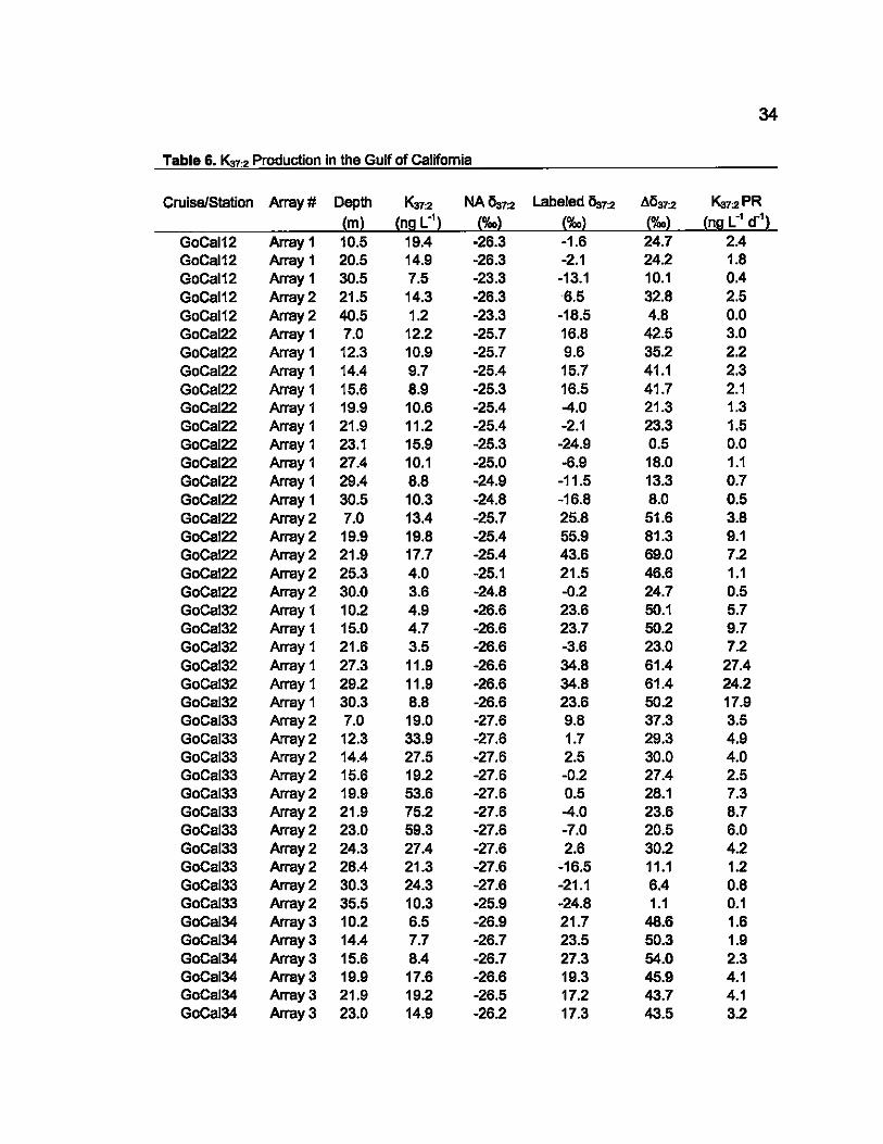
6. K:!7:2 Production in the Gulf of California ........................................... 34
7. A Comparison of Export Depth to the Depths of Maximum Concentration and Production in the Gulf of California ........................ 36
8. Integrated K:!7:2 Concentration and Production in the Gulf of California .................................................................................... 37
9. A Comparison of UK'37 Predicted Temperature with in situ Temperature ............................................................................. .41

v LIST OF FIGURES
Figure
1. Muller et al.. 1998 Core-top Dataset.: .............................................. 3
2. Map ofthe Gulf of Califomia .......................................................... 7
3. Goni et al.. 2001 Time-series Dataset... ........................................... 8
4. Water Column Profiles ................................................................ 19
K' 5. Depth Profiles of U 37 and 5i<37:2 ................................................... 20
6. Depth Profiles of Alkenone i<37:2 Concentration ................................. 32
7. Depth Profiles of i<37:2 Production Rates .......................................... 32
8. UK'37 vs. in situ temperatures ......................................................... 39
9. i<37:2 Photoperiod Growth Rate (P) vs. available light (PAR) ................. 41

CHAPTER 1 INTRODUCTION
1
Since their discovery and identification in sediments collected from Walvis
Ridge off West Africa [Boon et al. 1978] and the Black Sea [deLeeuw et al .•
1980]. alkenones (Car-Cas di-. trio. and tetraunsaturated methyl and ethyl
keytones) have been found to possess many characteristics that lend themselves
to be used as biomarkers. A1kenones in the open ocean are thought to be
produced exclusively by members of the Class Haptophyceae; most notably the
cosmopolitan species Emiliania huxleyi and the closely related Gephyrocapsa
oceanica [Marlow et al .• 1984a. b]. Unlike the majority of biologically synthesized
compounds. the chemical structure of alkenones contains the 'trans' double bond
configuration. which may help to prevent biodegradation in sediments [Rechka
and Maxwell. 1988a. b]. Most importantly for paleoceanographic applications.
the relative abundance of the double bonds in the compound has been found to
vary linearly with growth temperature (gT) of the biosynthesizing algae in
laboratory cultures [Prahl and Wakeham. 1987; Prahl at al.. 1988] and in the field
[Conte and Eglinton. 1993; Temois at al. 1997]. Focusing on the Ca7 alkenones.
Brassel et al. [1986] defined an alkenone unsaturation index (UKa7) that is
calculated from the relative abundances of the C37 methyl alkenones containing
2-4 double bonds.
UK37 = [C37:21-[Ca7:4]I[C37:2 + C37:3 + Ca7:4] (1 )

Because the concentration of the C37:4 alkenone is low in waters >15°C and the
C37:4 alkenone is rarely detected in sediments. Prahl and Wakeham [1987]
simplified UK37 to UK'37
UK' 37 = [C37:2lI[C37:2 + C37:3] (2)
and used the calculated UK' 37 and gT from batch culture experiments
(temperature range 8-25°C) to create a calibration curve that could be used to
quantitatively reconstruct ancient mean annual sea-surface temperature
(maSST) from deep-sea cores.
UK'37 = 0.033T + 0.043 (3)
2
This equation was determined using a specific strain of E. huxlayi (strain 55a or
CCMP 1742). and was later refined by Prahl at al. [1988] (UK'37 = O.034T + 0.039;
R2 =0.994). Further studies have shown that UK' 37 response to temperature can
vary depending on the species and strain of algae used [Temois at a/ .• 1997;
Conte et al.. 1998; Versteegh at al .• 2001]. Such genotypic differences could
decrease the applicability of using alkenones as a paleo-proxy for maSST. To
examine this further. Muller at al. [1998] and more recently Conte et al. [2006]
compiled UK'37 data for alkenones isolated from surficial sediments (core-tops)
collected on cruises throughout the world ocean and compared it to the maSST
for the region (temperatures were determined from the respective archives of the
NOAA World Ocean Atlas 1994 and the COADS archive for Muller at al. [1998]
and from the updated Levitus 2001 compilation for Conte at al. [2006]. see the
respective texts for more details). Remarkably. the calibration curves obtained
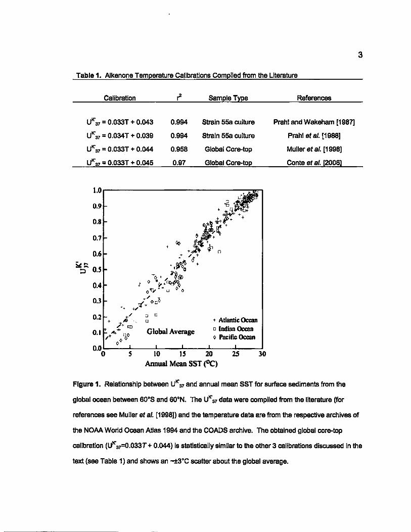
Tabla 1. Alkenone Temperature Calibrations Complied from the Literature
Calibration f Sample TyPe
UK' 37 = O.033T + 0.043 0.994 Strain 55& cultura
UK' 37 = O.034T + 0.039 0.994 Strain 55& cultura
UK' 37 = O.033T + 0.044 0.958 Global Core-top
UK' 37 = O.033T + 0.045 0.97 Global Core-top
1.0
0.9
0.8
0.7
0.6
5OI:::l~ O.S
0.4
0.3
0.2 +
0.1
0.0 0
4+
i~"( ~ +
t() • + ~ n
+ " t + ,;
d.~ t tl" a
~o • " .. ~~ .f ' .~.~
o't"',...~""o 0>0-
+" , .../+ (>0"
<!-. -+,1'''4-
" 0 c +,$ < u ,. '"
....... '/.,0 Global Average
+ Atlantic Ocean o Indian Ocean
0° Q P8l:ific Ocean
5 10 IS 20 2S Annual Mean SST ('Ie)
References
Prahl and Wakeham [1987)
Prahl et aI. [1988)
Muller et al. [1998)
Conte et aI. [2006)
30
Figure 1. Relationship between UK' 37 and annual mean SST for surface sediments from the
global ocean batween 60"S and 60"N. The UK' 37 data were complied from the litereture (for
3
references see Muller et al. [1998)) and the temperature data are from the respective archives of
the NOAA World Ocean Atlas 1994 and the COADS archive. The obtained global core-top
calibration (UK' ~.033T + 0.044) Is statisticelly similar to the other 3 calibrations discussed In the
text (see Table 1) and shows an -±3"C scatter about the global average.

4
from these data sets (UK'37 = 0,033T + 0.044; R2 =0.958 for Muller et aI, [1998]
and UK'37 = 0,033T + 0.045; R2 =0.97 for Conte et al. [2006]) are almost identical
to the Prahl and Wakeham [1987] and Prahl et al. [1988] calibration equations
(Table 1). Muller et al. [1998] concluded that strain 55a is similar enough to the
alkenone producing populations of the open ocean and apparent genotypic
differences seen in some culture experiments are not significant enough to
impede paleo-SST reconstruction. Despite the high statistical significance of
these relationships, considerable scatter is apparent in each of the core-top data
sets (e.g., see Fig. 1), which raises concern for paleo-temperature
reconstructions using the alkenone unsaturation index.
One possible ecological explanation for the scatter in the core-top data
could be that the alkenone producing populations grow and record water
temperatures at depths other than the surface mixed layer (SML). In fact, E.
huxley; is physically capable of migrating to and growing in the deepest parts of
the euphotic zone. Knappertsbusch [1993] found that E. huxley; can form
macroaggregates by secreting a polysaccharide that causes the algal cells to
coagulate. This macroaggregate could sink into the nutricline and allow cells to
continue growing because E. huxley; contains the accessory pigment 19'
hexanolyoxyfucoxanthin which enhances photosynthetic effectiveness in the
spectral range that penetrates deepest in the ocean [Haxo, 1985]. Field
evidence from various study sites such as the temperate northeast Pacific gyre
[Prahl et al., 1993], the Mediterranean Sea [Temois et al., 1997], the central

5
Pacific [Ohkouchi et al.. 1999]. and the Gulf of Maine [Prahl et al .• 2001] suggest
that the depth of alkenone export may be located beneath the SML. within a
deep chlorophyll maxima layer (DCML). at least during some periods of the year.
This ecological explanation could lead to an underestimate of SST for
reconstructions based on UK'37.
Scatter in the UK'3r-temperature relationship might also result from
physiological as opposed to ecological factors. Recent experiments by Epstein
et a/. [1998 and 2001] and Prahl et a/. [2003 and 2006] have shown that
physiological responses to nutrient and light availability can cause shifts in UK' 37
of ±0.13 (translates to approx. ±3°C). It has also recently been shown in field
experiments that algae growing in presumably nutrient limited waters in the
subtropical North Pacific contain alkenones that display a UK'37 index
systematically lower than expected based on any of the above-mentioned UK' 3r
temperature relationships. while algae growing deep in the water column under
lower light conditions contain alkenones that display a UK'37 index systematically
higher than in situ temperatures [Prahl et a/ .• 2005; Popp et a/ .• 2006a]. This
phenomenon may be related to the metabolic role that alkenones fulfill in the cell.
Originally it was believed that alkenones functioned as membrane lipids to
maintain fluidity as sterols do in other species [Brassell et a/ .• 1986]. but batch
culture experiments using 2 strains of E. huxlayi have shown that alkenones are
more likely energy storage molecules [Epstein at a/ .• 2001]. Traditional storage
lipids like triacylglycerols are conspicuously found only in very small quantities in

E. huxleyi, while alkenone concentrations are found in quantities similar to
triacylglycerol concentrations in other marine microalgae [pond and Harris,
6
1996]. As storage molecules, alkenone concentrations increase when the cells
are subjected to nutrient depleting conditions (e.g., at the end of a bloom)
because nitrogen and phosphorus are not available to biosynthesize proteins and
nucleic acids. On the other hand, alkenone concentrations decrease when cells
are subjected to low light levels (e.g., deep in the euphotic zone) because the
algae are burning the energy stored in the alkenones to continue growth with the
available nutrients [Prahl et a/., 2003]. Preferential degradation of the higher
energy C37:3 alkenones during light deprivation, and preferential biosynthesis of
the higher energy C37:3 alkenones during nutrient depletion could explain the
observed UK" 37/gT discrepancy observed in the laboratory [Epstein et a/. 1998;
2001; Prahl et a/. 2003; 2006] and in the field [Prahl et a/. 2005; Popp et al.
2006a].
An understanding of the growth conditions of E. huxleyi, especially in light
of the additional ecological and physiological factors that can affect UK" 37, could
help explain some of the observed variability in the core-top calibrations of Muller
et a/. [1998] and Conte et al. [2006] (Fig. 1) and could ultimately improve the
accuracy of the UK" 37 index as a paleoSST proxy. The study site chosen for this
investigation was in and around the Guaymas Basin, Gulf of California (Fig. 2)
due to its unique physical oceanographic environment that allows for a wide
range of sampling conditions. Because of seasonal changes in wind patterns,

-116" ." "
km -G :Ie 100
Figure 2. Map showing the location in the Gulf of California where the 4 sampling sites are
situated.
surface waters in the Gulf of California are characterized by stratification in the
summer and strong upwelling in the winter. These changes in wind stress result
in large seasonal changes in SST and in nutrient dynamics [Zineri and Thurnell,
2000; Thunell , 1998 and references therein). Surface temperatures can be as
low as 15°C during winter months due to the strong northwesterly winds that
blow down the axis of the Gulf and induce deep mixing of the water column. In
the summer, the wind pattern reverses, causing weak upwelling along the
western Gulf and strong thermal stratification in the eastern and central Gulf.
Sea surface temperatures during summer stratification can exceed 30°C while
nutrient levels drop significantly. Although total primary productivity in the
7

8
Guaymas Basin maximizes during upwelling and minimizes during stratification
[Thunell, 1998], sediment trap time series analysis from January 1996 to
September 1997 provided by Goni et al [2001] showed that alkenone flux
maximized during the summer and minimized in the winter.
A previous study in the Gulf of California [Goni et ai, 2001], which
collected alkenone concentration and UK' 37 values from surficial sediments and a
sediment trap deployed at 500 m from January 1996 to September 1997, found
that although the measured UK'37 values correlated well with SST measured
using Advanced Very High Resolution Radiometry (AVHRR) data for the majority
of the data set, at SST>26°C, values for UK'37 were systematically lower than
0 ., ~ .... • M
~
1 -;---"-'--~ • , !
~ A/ I
ae i • • • ae
07
05 ,. '6 18 ~ ~ ~ ~ ~ ~ ~ ~
AVHRR Tempem1ure (0 C)
Figure 3. Adapted from Gonl et aJ. [2001]. Plot of AVHRR temperature vs. UK' 37 ratios for
sediment trap samples. Line A represents the expression derived by Prahl et al. [1988] and Line
B represents the nonlinear fit to the data using a 31d order polynomial expression described in
Gonl et al. [2001].

9
expected based on the UK'3rtemperature relationship of Prahl et a/. [1988) (Fig.
3). This -3°C deviation from the UK'3rtemperature relationship is reminiscent of
the observed variability in the Muller et a/. [1998) and Conte et al. [2006) core-top
calibrations. Three possible explanations for this discrepancy were offered by
Goni et a/. [2001):
1) The physiological response to gT of the alkenone producing
community present in the Gulf of Califomia might not be the same as
documented for the E. huxleyi strain used to develop the calibration
equation of Prahl and Wakeham [1987). Conte et al. [1998) found
strains of E. huxleyi and G. oceanica, isolated from the Sargasso Sea
and SW Pacific respectively, which show a similar non-linear response
to growth temperature.
2) The community of alkenone producers might vary throughout the year.
Ziveri and Thumell [2000) documented seasonal changes in algal
community in the Gulf of California. Production flux was dominated by
E. huxleyi when SST <27°C, while the dominant flux contributor for
SST>2~C was G. oceanica. Even if both species have a linear
physiological response to gT, the UK'37 calibration equations need to be
statistically the same in order for accurate paleoreconstruction of
maSST from the underlying sediments.
3) The export depth of the alkenone producing community might not be
within the SML throughout the year. When the SST in the Gulf of
10
California is large. strong thermal stratification occurs in the euphotic
zone. UK·37 values that translate to a gT <SST could have resulted from
alkenone production occurring deeper in the water column. within the
thermocline and below the SML.
Taking into consideration the results of Epstein at a/. [1998 and 2001] and Prahl
at a/. [2003 and 2006]. a 4th explanation is now offered:
4) The UK' 37 values synthesized during the warm summer months might
underestimate gT by up to 3·C because of nutrient limitation. Previous
studies in the Gulf of California [Gaxiola-Castro at a/. 1999; White et al.
2007] found that nitrate concentrations are undetectable during the
summer in the SML.
In the present study. alkenone unsaturation patterns (UK'37). alkenone-specific
carbon isotopic variation (lSKa7:2). and seasonal alkenone concentration and
production rate are determined throughout the upper water column (0-40 m) in
the Gulf of California in order to better constrain the depth of alkenone export
production and to identify factors that might cause calculated UK·37 temperatures
to underestimate SST when SST>26°C. Field data were collected during one
wintertime (January - February 2005) and two summertime (July 2004 & July
August 2005) cruises. Alkenone production rates were determined using an in
situ l3C incubation method utilized in a related study in the subtropical
oligotrophic North Pacific [Prahl at a/ .• 2005; Popp at sl .• 2006a]. which was
originally modified after that employed previously in the Sea of Japan [Hamanaka

11
at al., 2000] and the Bering Sea [Shin et a/., 2002]. Alkenone export production
was determined to originate from a depth of -20-30 m, which is well below the
SML during the summer. Exported UK'37 did underestimate SST by up to -3°C,
but this underestimate was not as large as expected based on the temperature
gradient between the SML and the depth of export, and probably resulted from a
concurrent physiological response to growth under light limiting conditions. As a
result, SST estimates made by measuring UK' 37 fall within the ±3°C variability
observed in the core-top calibrations of Muller at a/. [1998] and Conte at al.
[2006], indicating that subsurface alkenone growth could still lead to relatively
accurate SST predictions (Le. within ±3°C). Additionally, the efficiency of
alkenone export production to sediment traps deployed at 100 m is determined to
be -20%. This alkenone export efficiency is the first measurement of this type to
be reported in the literature and implies considerable loss of alkenones probably
due to the effects of grazing.

2.1. Sampling site
CHAPTER 2 SAMPLES AND METHODS
12
Samples were collected and experiments performed in and around the
Guaymas Basin, Gulf of California (27°30'N, 111 °20'W) aboard the 'RV New
Horizon during one wintertime (January - February 2005) and two summertime
(July 2004 & July - August 2005) cruises. GoCal1 (July 7-23,2004) and GoCal2
(January 25 - February 10, 2005) occurred exclusively within Guaymas Basin
(station 2), while GoCal3 (July 23 - August 13, 2005) also visited 3 other stations
(3-4, 1) in the Gulf for comparative stUdies (Fig. 2).
2.2. Suspended particulate material samples
Samples of suspended particulate material (SPM) were collected
throughout the upper water column (-0-80 m in GoCal1, -40 m in GoCal2 and
GoCaI3). Large volume (-80 L) seawater samples for alkenone analysis were
collected approximately every 5 m by closing multiple 10-L PVC sample bottles
on a CTD rosette during dedicated CTD casts. For each depth, water collected
was pressure filtered (-10 psi) through a single precombusted glass-fiber filter
(148 mm or 90 mm dia. Whatman GF/F or Millipore APFF, each 0.7 pm nominal
pore size) and stored frozen (-20°C) until processed for gas chromatographic
analysis of alkenones using both flame ionization detection (GC-FID) and
compound specific stable isotopic analYSis (irmGCMS).
Samples for nutrients (nitrate/nitrite, phosphate, and silicate), total
alkalinity (T A), and total dissolved inorganic carbon (DIC) concentration and

13
isotopic analysis were also obtained from dedicated CTD casts. Samples for DIC
isotopic analysis were collected without aeration in 20m I glass serum vials,
preserved by addition of HgCI2 (5pl of saturated solution), sealed with a butyl
rubber stopper and stored under darkness at room temperature for later
laboratory analysis. Samples for DIC were collected in 300 mL glass bottles with
ground-glass stoppers in a similar manner. Samples for T A analysis were
collected and handled similarly, but without the addition of HgCI2 [Karl et al.,
1990]. Nutrient samples were collected in pre-cleaned polyvials directly from the
PVC sample bottles on the Rosette and stored frozen (-20°C) for later analysis in
the laboratory as well. Light attenuation coefficients for photosynthetic active
radiation (PAR) were obtained using PAR data collected during daytime CTD
casts. Water column profiles of photosynthetic active radiation (PAR) were
calculated as described by Popp et al. [2006a] using SeaWiFS-derived 8-clay
average 27-km surface PAR that coincided with the timing of our in situ
experiments.
2.3. Free floating arrays
Water samples for incubation experiments were collected and handled
following the protocols of Prahl et al. [2005] and Popp et al. [2006a]. Water for
each incubation depth was transferred into polycarbonate carboys and a 13e
labeled bicarbonate solution added. The carboys were then attached to an in
situ array, deployed before dawn, and allowed to drift freely for 24 hours before
recovery. Upon retrieval, samples were taken from each carboy and processed

14
as described for DlC isotopic analysis to confirm the level of isotopic enrichment.
Remaining water volumes were then pressure filtered and processed as
described for SPM material.
2.4. Sediment trap samples
Passively settling particulate matter was collected by attaching twelve
VERTEX-style traps to the free-floating array (-100 m depth) following the
protocol of Knauer et a/. [1979]. Upon retrieval, the particulate matter from one
trap was combined onto a single 25 mm precombusted glass-fiber filter and
processed for analysis of POM and PN as described by White et al. [2007]. The
remaining traps (cross sectional area = 0.0039 m2/trap) were combined for
alkenone analysis and filtered as described above for SPM samples.
2.5. Analytical techniques
At Oregon State University (OSU), alkenone fractions were isolated from
the sediment trap, incubation, and SPM samples using established ultrasonic
solvent extraction and column chromatographic methods [Prahl et al., 1989].
The precision of absolute alkenone concentrations and alkenone unsaturation
(UK'37) values were better than ±10% and ±0.01, respectively. Alkenone fractions
were then saponified [Christie, 1973] and sent to the University of Hawaii for
compound specific carbon isotopic analysis by irmGCMS [Hayes et al., 1990].
Natural abundance (SPM and sediment trap) and isotopically labeled
(incubation) samples were chromatographically purified using a TraceGC

15
equipped with a cool, on-column injector and a J&W Scientific DB-1MS column
(60-m x 0.32-mm x 0.25-pm) that was temperature programmed from 60 to
320°C at 1Q°C min"' prior to on-line isotopic analysis using an MAT 252 isotope
ratio monitoring gas chromatograph mass spectrometer (irmGCMS). Precision of
replicate irmGCMS analyses of natural abundance samples ranged from ±0.04 to
±0.53%o but averaged ±0.27%O, while isotopically labeled sample values ranged
from ±0.01 to ±2.2%O and averaged ±0.66%. For the purpose of error
propagation, conservative values of ±0.5 and ±1.0o/oo were used for the precision
of analysis, respectively.
~'3CDlC values were determined at the University of Hawaii (UH) using a
Gasbench interfaced to a Delta XP mass spectrometer. Typical precision for
replicates was better than 0.2%0. DIC concentrations were determined
coulometerically at UH using a Single-Operator Multi-Metabolic analyzer
(SOMMA) system similar to that described by Johnson et a/. [1993]. Total
alkalinity was determined by the Gran method [Gran, 1952] using computer
controlled titration at UH as well. Precision of replicate samples was better than
±5 jJeq kg"'. Nitrate+nitrite and phosphate concentrations were analyzed at OSU
using the colorimetric techniques of Strickland and Parsons [1972] on an AJpkem
"Flow Solution" Autoanalyzer continuous flow system. Silicate concentrations
were determined according to the method of Armstrong et a/. [1967] as adapted
by Atlas et a/. [1971]. The detection limits (and coefficients of variation) for

nitrate, phosphate. and silicate measurements were 0.1 pmol L-1 (0.2%), 0.2
pmol L-1 (1 %), and 0.3 pmol L-1 (0.5%), respectively.
16
Alkenone production and photoperiod growth rates were calculated from
the change in the 13e atom percent of the alkenones and e02(aq) measured after
incubation as described by Popp at a/. [2006a, b). The 13e at. % of alkenones
was corrected for the 4.2%0 isotope offset between the alkenone and the primary
photosynthate that is associated with biosynthesis and for isotopic fractionation
associate with fixation of e02(aq) [Popp et al., 1998). e02(aq) 13e at. % was used
to calculate production rates instead of the ole 13e at: % which was used in a
previous study [see Hamanaka et al., 2000) because e02(aq) is the primary
inorganic carbon substrate utilized by E. huxley; [Rost et a/., 2003).
e02(aq) 13e at. % was calculated from ~13eDlC values and the relative
abundances of the various carbonate species determined using the e02SYS
program developed by Lewis and Wallace [1998). This program (available at
http://cdiac.oml.gov/oceans/co2rprt.html) calculates the species distribution of
the carbonate system from salinity, temperature, depth, TA, and the
concentrations of Ole, phosphate, and silicate. The dissociation constants for
KS04, B(OHh, and H2e03 used in this calculation were adopted from Dickson
[1990a, 1990b) and Mehrbach et a/. [1973) as refit by Dickson and Millero [1987).
The temperature fractionation relationships used to calculate e02(aQ) 13e at. %
were taken from Deines et al. [1974] and Mock et al. [1974]. Propagated errors
for alkenone production and growth rate calculations were approx. 10% of the
given rate.

CHAPTER 3 RESULTS AND DISCUSSION
3.1. Water column properties
17
Water column profiles of relevant properties are presented for each station
in Figure 4. Conditions in the Gulf of Califomia varied both by season (a-o) and
by location (o-f). The depth of the SML varied from 32-40 m during the winter
cruise (GoCaI22, Fig. 4b) and from <5 m (GoCa131, Fig. 4f) to -16 m (GoCa132
and GoCal34, Fig. 4c and 4e, respectively) in the summer cruises. Dissolved
inorganic nitrogen (NO£ + N03-) was below the detection limit (0.1 pmol L-1) in
surface waters during the summer, but increased rapidly below 40 m. Surface
PAR values ranged from 1139 pEin m-2 S-l (GoCaI32, Fig. 4c) to 1215 pEin m-2 s-
1 (GoCal34, Fig. 4e) in the summer and was approximately 905 pEin m-2 S-l in the
winter. Light attenuation coefficients varied with station and ranged from 0.075
m-1 in the winter to 0.178 m-1 in the summer (Table 2). In general, PAR
decreased exponentially with increasing water depth (Fig. 4) with the greatest
attenuation of light occurring at Station GoCal12 (Fig. 4a).
3.2. Depth of Alkenone Export
Depth of alkenone export in the Gulf of Califomia can be constrained to an
approximate range at each cruise/station by comparing the depth profiles of
alkenone unsaturation (UK•37) values and alkenone-specific carbon isotopic
composition (5Ka7:2) with similar measurements in material collected in the
sediment traps. Systematic variations with depth in the water column of each

Table 2. Photosynthetic_Active Radiation (PAR) In the Gulf of california
Cruise/Station Date Photoperiod k sPAR PAR...ro PARzo2Q PARzo30
(hrs) (m·1) wEin m·2 s·1) wEin m-2 S·1) wEin m·2 S·1) wEin m·2 S·1)
Gocal12 7/1412004 13.72 0.1785 1168.2 196.1 32.9 5.5 GoCaI22 1/3112005 10.87 0.0746 904.6 428.9 203.4 96.4 GoCal32 712912005 13.49 0.0836 1138.7 493.6 213.9 92.7 GoCal33 8/112005 13.58 0.0955 1151.6 443.4 170.7 65.7 GoCaI34 81412005 13.31 0.0982 1214.6 454.9 170.4 63.8 GoCal31 81612005 13.30 0.1025 1196.7 429.3 154.0 55.2
where k is the diffuse light attenuatlon-coefficent, sPAR is PAR at the surface, and PAR. is PAR at that respective depth calculated by the equation: PAR.=sPAR*e.Jcz
..... 00

(a)
o
20
I 40
'" -a 60 ~
C
80
Temperature (DC)
1416182022 24 2628 30 32
. N~N '(~';'O'I k~ -1') ,
o 5 10 15 20 25
• ~ • •
- PAR ---4- N+N
100 1# • Temperature
(d)
20
40
;; g- 60 c
80
100
o 200 400 600 800 1000
PAR (~E i n m-2 s-l )
Temperature (ee )
1214 16 1820 22 24 26 28 30 32
' N~N (~OI 'k9~ 1 ) ' ,
o
•
•
5 10 15 20 25
•
~ -• - • . -
o 200 400 600 800 1000
PAR (J,LEin m·2 5.1)
(b)
o
20
40
I a 60 • c
80
100
(e)
Temperature ('"C)
14 15 16 17 18 19 20
N+~ (~I k~·1 ) o 5 10 15 20 25
- PAR ~ N+N
• Array2 e. . . Array1
o 200 400 600 BOO
PAR ().lEin mo2 s·1)
Temperature ('C)
14 16 1820 22 24 26 28 30 32
20
I 40
'" C. 60 c3
60
100
o
N+N (';"'~ I kg-l) ,
• •
5 10 15 20 25
•
. 1· ...: ••• -• ••
o 200 400 600 800 1000
PAR (~E in m-2 s-l)
(c)
20
80
Temperature (DC)
14 16 18 20 22 24 26 28 30 32
N+N (.mol kg-1)
o 5 10 15 20 25
•
•
. ----100 ..
(I)
o 200 400 600 800 1000
PAR (jlEin m-2 s·1)
Temperature (0C)
16 18 20 22 24 26 28 30 32
N~N (~Ol 'k9:1) ,
-2024681012141618 o •
r 20
I 40
'" C. 60 ~
C
80
lOa ••
• •
•
-• •• ...
o 200 400 600 800 1000
PAR (.ein m-2 s-l )
Figure 4. Water column profiles of available light (PAR), dissolved inorganic nitrogen (NO; +
NO,-) and temperature for GoCal12 (a), GoCal22 (b), GoCal32 (c) , GoCal33 (d), GoCal34 (e),
and GoCal31 (f). The temperature profile in GoCal22 was slightly different for each incubation
experiment.
19

parameter are necessary to constrain the depth of alkenone export. For each
station/cruise in the present study, at least one of the two parameters shows a
sufficient range in values for comparison to the sediment trap values with the
exception of the winter cruise (GoCaI22) (Fig. 5). We assumed that UK'37 and
OK372 values measured in the sediment trap material reflect the depth of
alkenone export production , Additional assumptions are that there are no
changes in these parameters during export and that lateral inputs of alkenones
(a) (b)
0 0 • • '.. 4 . .. · \ · "f . .' • • 20 i' ~, 20 . • ". =.~ • to' ' .. • . ..,' • • • • • • • · . • • • • • • • • .~
I 4<l t • I 40 • • • • £ • ~
Q, 60 • GC22 li 60 Q GC32 Q GoCal32 C C
• GC12 • GoCaI33 80 • 80 • GoCat34
• GoCal31
100 , , .. 100 · . • • 0.5 0 .• 0.7 0.8 0 .• 1.0 0.60 0.85 0.90 0.95 1.00
UK'37 UK'37
(c) (d)
0 0 • • • • • • . - , • • • • • ,
20 • ~. • • 20 • • • .. -: .... • • • • • , . • • · • • • . • • •
I 40 I 40 • • • • £ ~
Q, 60 li 60 0 Q
C C
80 • 80
100 . .. , , 100 • • • • ·28 ·27 ·26 ·25 ·24 ·23 ·22 ·29 ·28 ·27 ·26 ·25 ·24
8K37:2 6K37,2
Figure 5. Depth profiles of alkenone unsaturation patterns (UK'37) for station 2 (a) and cruise 3
(b) and alkenone·specific carbon isotopic patterns (i5K37'2) for station 2 (c) and cruise 3 (d).
Respective UK'37 and i5K37,2 values obtained from the sediment traps are plotted at the 100m
collection depth for comparison to the overlying water column profiles.
20

21
are relatively minor. Grice at a/. (1998) found that there was no alteration in UK' 37
or riK:!7:2 as a function of zooplankton grazing.
Alkenone unsaturation pattems (UK'37) were determined for all SPM,
incubation, and sediment trap samples (Table 3). Depth profiles ofthe UK'37
index for each cruise/station are shown in Figure 5a-b. Values ranged from
0.587 in the winter (Fig. 5a) and reached maximum values of the UK' 37 index of
1.000 in the summer (GoCaI31, Fig. 5b). A UK
'37 index of 1 indicates that the K:!7:3
species was undetectable in the water column. At station 2, the GoCal12 UK'37
depth profile shows considerably more scatter than the GoCal32 profile, but both
show the same general trend of steadily decreasing UK' 37 values with increasing
depth (Fig. 5a). No trend with respect to depth is observed in the GoCal22 UK' 37
data (Fig. 5a), but since the SML extends to -40 m in the winter and
temperatures are relatively constant throughout this range, this result is not
unexpected. With respect to the other stations visited in Cruise 3, the observed
UK' 37 depth profile of GoCal32 is very similar to GoCa133, but GoCal34 and
GoCal31 appear quite different (Fig. 5b). The magnitude of the variation in UK'37
with depth seen in GoCal32 and GoCal33 is significantly reduced at the other 2
stations. From -0-30 m UK' 37 remains relatively constant, and then begins to
decrease at greater depths.
Alkenone-specific carbon isotopic values (riK:!7:2) of the SPM and sediment
trap samples were also determined (Table 3). Natural abundance isotopiC
variation between all cruises/stations ranged from -28.70/00 to -22.4%0. Depth

22
Table 3. Alkenone Unsaturation (UK'37) and Natural Abundance Carbon Isotopic (6:17:2) Pattems in the Gulf of Califomia
Cruise/Station Sample Type Depth UK'37 NA6:l72 (m) %0
GoCal12 CTD Rosette 7.8 0.993 -25.27 GoCal12 CTD Rosette 10.3 0.983 -26.20 GoCal12 CTD Rosette 10.4 0.993 -26.75 GoCal12 In situ Pump 10.4 0.987 -25.97 GoCal12 CTDRosatte 10.4 0.994 -25.87 GoCal12 CTDRosatte 10.4 0.997 -27.11 GoCal12 Array 1 10.5 0.982 GoCal12 CTD Rosette 18.2 0.972 -26.40 GoCal12 Array 1 20.5 0.906 GoCal12 Array 2 21.5 0.915 GoCal12 CTD Rosatte 25.1 0.947 -23.36 GoCal12 In situ Pump 25.4 0.803 -22.97 GoCal12 CTD Rosette 25.5 0.946 -23.51 GoCal12 CTD Rosette 25.6 0.954 -23.72 GoCal12 CTD Rosette 25.7 0.945 -22.75 GoCal12 CTD Rosette 27.3 0.908 -22.65 GoCal12 CTD Rosette 27.5 0.934 -22.44 GoCal12 CTD Rosatte 27.6 0.955 -23.92 GoCal12 CTD Rosatte 28.9 0.905 -23.34 GoCal12 Array 1 30.5 0.850 GoCal12 CTD Rosette 35.7 0.818 -23.04 GoCal12 CTD Rosette 35.7 0.858 -22.59 GoCal12 Array 2 40.5 0.855 GoCal12 CTD Rosette 40.8 0.886 -23.92 GoCal12 CTD Rosatte 41.1 0.859 -23.46 GoCal12 CTD Rosette 51.0 0.829 -23.90 GoCal12 CTD Rosette 80.5 0.897 -23.21 GoCal12 SedIment Trap 100.0 0.957 -25.41 GoCal12 Sediment Trap 100.0 0.943 -25.25 GoCaI22 Array 1 7.0 0.621 GoCaI22 Array 2 7.0 0.657 GoCal22 CTD Rosatte 11.6 0.621 -25.74 GoCaI22 Array 1 12.3 0.657 GoCaI22 Array 1 14.4 0.658 GoCaI22 Array 1 15.6 0.662 GoCaI22 CTD Rosette 16.4 0.587 -25.19 GoCal22 Array 1 19.9 0.655 GoCaI22 Array 2 19.9 0.6n GoCaI22 CTD Rosatte 21.6 0.603 -25.39 GoCal22 Array 1 21.9 0.660 GoCal22 Array 2 21.9 0.674 GoCaI22 Array 1 23.1 0.599 GoCaI22 Array 2 25.3 0.637

23
Table 3. (Continued) Alkenone Unsaturatlon (UI< 37) and Natural Abundance Carbon Isotopic (!5a7:2) Patterns In the Gulf of California
Cruise/Station Sample Type Depth UI<37 NA !5a7:2 (m) %0
GoCeI22 cm Rosette 27.0 0.619 -25.02 GoCal22 Array 1 27.4 0.651 GoCal22 Array 1 29.4 0.636 GoCal22 Array 2 30.0 0.694 GoCeI22 Array 1 30.5 0.644 GoCal22 CTD Rosette 32.0 0.635 -24.71 GoCal22 CTDRosette 36.6 0.639 -24.43 GoCal22 Sedlmant Trap 100.0 0.615 -22.91 GoCal22 Sediment Trap 100.0 0.660 -23.84 GoCel32 cm Rosette 6.3 0.996 -26.56 GoCel32 Array 1 10.2 0.994 GoCal32 CTD Rosette 11.2 0.985 -26.75 GoCel32 Array 1 15.0 0.991 GoCel32 CTD Rosette 16.6 0.976 -26.40 GoCal32 Array 1 21.6 0.962 GoCel32 CTD Rosette 26.5 0.935 -26.50 GoCel32 CTD Rosette 26.5 0.948 -26.45 GoCal32 Array 1 27.3 0.924 GoCel32 Array 1 29.2 0.908 GoCal32 Array 1 30.3 0.946 GoCal32 cm Rosette 31.8 0.937 -26.79 GoCel32 cm Rosette 36.8 0.859 -25.66 GoCal32 cm Rosette 42.8 0.857 -25.61 GoCal32 Sediment Trap 100.0 0.945 -25.72 GoCeI33 cm Rosette 6.0 0.999 -27.61 GoCel33 Array 2 7.0 0.993 GoCeI33 cm Rosette 11.4 0.997 -27.54 GoCeI33 Array 2 12.3 0.995 GoCeI33 Array 2 14.4 0.994 GoCeI33 Array 2 15.6 0.999 GoCeI33 cm Rosette 18.5 0.965 -27.61 GoCel33 Array 2 19.9 0.939 GoCel33 Array 2 21.9 0.936 GoCal33 Array 2 23.0 0.920 GoCel33 CTD Rosette 23.9 0.902 -27.50 GoCel33 Array 2 24.3 0.800 GoCal33 cm Rosette 26.8 0.972 -27.65 GoCel33 Array 2 28.4 0.802 GoCel33 Array 2 30.3 0.845 GoCel33 CTD Rosette 31.4 0.854 -27.56 GoCel33 Array 2 35.5 0.874 GoCal33 cm Rosette 36.7 0.843 -25.68 GoCal33 CTD Rosette 40.4 0.841 -25.08

24
Table 3. (Continued) Alkenone Unseturetion (UK' 37) and Natural Abundance Garbon Isotopic (1537:2) Patterns in the Gulf of California
Cruise/Station Sample Type Depth K' U 37 NA 1!a7:2
(ml 0/00 GoCal33 Sediment Trap 100.0 0.935 -26.52 GoCal34 CTD Rosette 6.8 0.995 -26.99 GoCal34 Array 3 10.2 0.970 GoCal34 CTD Rosatte 11.6 0.981 -25.74 GoCaI34 Array 3 14.4 0.993 GoCaI34 Array 3 15.6 0.992 GoCaI34 CTD Rosette 16.4 0.997 -25.84 GoCaI34 Array 3 19.9 0.998 GoCaI34 Array 3 21.9 0.995 GoCal34 CTD Rosette 22.0 0.998 -26.50 GoCal34 Array 3 23.0 0.992 GoCal34 Array 3 24.3 0.995 GoCaI34 CTD Rosette 24.4 0.997 -25.82 GoCaI34 Array 3 28.4 0.986 GoCal34 Array 3 30.3 0.992 GoCaI34 CTD Rosatte 31.5 0.987 -24.99 GoCaI34 Array 3 35.5 0.914 GoCaI34 CTD Rosette 36.8 0.978 -26.72 GoCal34 CTDRosatte 41.7 0.960 -24.42 GoCaI34 Sediment Trap 100.0 0.961 -25.42 GoCal31 CTD Rosatte 6.2 0.992 -28.69 GoCaI31 Array 4 8.1 0.997 GoCal31 CTDRosatte 11.6 0.994 -28.61 GoCal31 Array 4 12.3 1.000 GoCaI31 Array 4 14.4 0.999 GoCal31 Array 4 15.6 0.999 GoCal31 CTDRosatte 16.8 0.997 -28.46 GoCal31 Array 4 19.9 0.993 GoCal31 CTD Rosette 21.5 0.992 -27.66 GoCal31 Array 4 21.9 0.993 GOCal31 Array 4 23.0 0.995 GoCal31 Array 4 24.3 0.979 GoCal31 CTD Rosatte 26.6 0.984 -26.23 GoCal31 Array 4 28.4 0.981 GoCal31 Array 4 30.3 0.983 GOCal31 CTD Rosatte 31.7 0.989 -25.43 GoCal31 Array 4 35.5 0.983 GoCal31 CTD Rosatte 36.6 0.985 -25.30 GoCal31 CTD Rosatte 41.6 0.973 -24.84 GoCal31 Sediment Trap 100.0 0.972 -25.91

25
profiles of 151<J7:2 for each cruise/station generally increased with increasing depth
(Fig. 5c-d), but showed distinct differences between each cruise/station. Unlike
the observed UK'37 patterns, GoCaI12151<J7:2 differs significantly from GoCal32
15K37:2 (Fig. 5c). The depth profile of 151<J7:2 in GoCal32 remains relatively
constant (--26.6o/OQ) until a depth of 35 m and then increases -1 %.. In contrast,
GoCaI1215~7:2 values above 25 m cluster around -26.3%0 while those below
cluster around -23.3%., a dramatic -3%. shift. This shift is probably not caused
by changes in the alkenone-producing community. During GoCa112, the surface
waters were dominated by G. oceanica, while E. huxley; dominated at depth, but
during GoCa133, E. hux/eyi dominated at the surface and G. ocaanica dominated
at depth [Malinvemo et a/., in prep.1. If the -3%0 shift in the 151<J7:2 observed
during GoCal12 (Fig. 5c) reflects only a change in species distribution where
more negative 151<J7:2 values are attributed to greater abundance of G. ocaanica,
then 151<J7:2 values would be expected to decrease with increasing depth at
GoCa133. The opposite is observed at this station (Fig. 5d) indicating that the
shifts in 151<J7:2 values are not related only to a change in the species of alkenone
producing algae. A more likely cause of the -3%0 shift during GoCal12 (Fig. 5c)
is an effect of light limitation on carbon isotopic fractionation in the alkenone
producing algae. Rost et a/. [20021 documented an isotopic shift of up to 8%0 as
a result of E. hux/eyi grown in dilute batch cultures under conditions of limiting
light. If a similar effect is occurring during the present study, then an increase in
151<J7:2 values with respect to increasing depth might be expected. The fact that

26
isotopic values at the 3 remaining stations (GoCa122, GoCal34, and GoCa131) all
steadily increase with increasing depth with net changes of -1.40/00, 2.60/00, and
3.9%0 respectively (Fig. 5c-d), further support the explanation of Iight-dependent
isotopic fractionation. The lack of systematic variation with respect to depth
during GoCal12 (Fig. 5c) could simply be due to the fact that available light at
GoCal12 diminished more quicker in the water column than at the other
cruise/stations (Fig. 4 and Table 2).
Values of UK' 37 and 15Ka7:2 determined from the sediment trap material are
plotted at the 100 m collection depth in Figure 5 for comparison to the water
column profiles of each parameter. Corresponding depths derived from both
parameters of each cruise/station are presented in Table 4. Depths shown in
bold typeface indicate the parameter that shows the greatest magnitude of
systematic variation with respect to depth in the water column, and are therefore
capable of yielding the most precise estimate of the 2 depth extrapolations for
that given cruise/station. For example, the GoCal12 UK" 37 values (Fig. Sa) span a
wide range and encompasses both UK'37 sediment trap values. Corresponding
water column depths for the trap UK'37 are -26 m. On the other hand, the
GoCal12 15Ka7:2 values consist of 2 distinct clusters (Fig. 5c) that do not show
sufficient systematic variation within each cluster to pinpoint a specific depth of
inferred alkenone export production. Therefore the sediment trap 15Ka7:2 values of
-25.40/00 and -25.30/00 can only constrain the depth of alkenone export production
to the upper 25m of the water column.

Tabla 4. Alkenone Export in the Gulf of California
Cruise/Station Array # uK'arDepth !5:r,:TDepth Export Depth SMLDepth UK'3T"T SML-T UK'37"'T-SML-T ED-T ED-T-SML-T (m) (m) (m) (m) (OC) (OC) (OC) (OC) (OC)
GoCal12 Array 1 25.3 0-25 20-25 15 27.3 29.0 -1.7 23.1 -5.9 GoCaJ12 Array 2 28.5 0-25 20-25 15 26.8 29.0 -2.2 23.1 -5.9 GoCaJ22 Array 1 7-27 60.3 20-30 40 18.4 18.7 -0.3 18.6 -0.1 GoCai22 Array 2 12-22 45.8 20-30 32 17.0 18.7 -1.7 18.6 -0.1 GoCaJ32 Array 1 28.4 36.5 25-30 16 26.9 29.2 -2.3 23.2 -6.0 GoCaJ33 Array 2 21.1 34.3 20-25 6 26.6 29.8 -3.2 22.4 -7.4 GoCaI34 Array 3 41.4 28.8 25-30 16 27.4 29.9 -2.5 27.0 -2.9 GoCal31 Array 4 42.8 28.7 25-30 <5 27.7 30.3 -2.6 26.1 -4.2
Where UK' 3T" T is calculated from the sediment trap-derlved UK' 37 using the calibration of Conte et a/. [2006)
!::i

28
The most likely depth of export for each cruise/station is determined by
taking into consideration the 2 export depth predictions obtained by comparing
sediment trap UK' 37 and li1<J7:2 to the natural variation in the overlying water
column (i.e. 26 m for UK' 37 and 0-25 m for li1<J7:2 in GoCa112) (Table 4). Since the
GoCal12 UK'37 depth extrapolation is better constrained, a depth of alkenone
export production of 20-25 m is a reasonable estimate for this cruise/station (see
Table 4). Using this approach, the estimated depth of alkenone export
production was determined to be 20-25 m for GoCal33 and 25-30 m for GoCal32,
GoCal34, and GoCal31 (Table 4). Export depth for the winter cruise (GoCal22)
is the most difficult to ascertain because of the lack of systematic variation in the
UK' 37 water column profile (Fig. 5c) and because the sediment trap li1<J7:2 values
fall outside the range of values measured in the water column (Fig. 5d). liKs7:2
profile extrapolation leads to very deep export depths (>45 m), while the possible
range indicated by the UK·37 scatter is much shallower (10-30 m) (Table 4). The
cause for this discrepancy is unknown but for the purposes of this investigation, it
is assumed that the export depth in the winter at station 2 is relatively similar to
the summer export depths (Le. 20-30 m).
Using the sediment-based UK·3rtemperature relationship of Conte at a/.
[2006], UK' 37 values of the sediment trap samples can be converted into growth
temperatures (gTs). These predicted temperatures are then compared to the in
situ temperature of the SML (as determined from the CTD downcast data files) in
order to determine how well exported UK" 37 values record SST (Table 4). In all

29
cases, the temperature of the SML (SML-7) is underestimated by the UK' 3r
temperature prediction (indicated by a '-' value in Table 4). The magnitude of
the underestimation was relatively small for the winter cruise (0.3°C for GoCal22
array1), but was as large as 3.2°C for GoCal33 (fable 4). Interestingly, this
magnitude of variation is similar to the magnitude of scatter observed in the
Muller et al. [19981 and Conte et al. [20061 coretop UK' 3rSST relationship. In
other words, sediment trap-derived UK' 37 temperatures in the Gulf of California
systematically underestimates in situ SML temperatures, but the underestimation
falls within the observed variability of the method. This -3°C temperature
underestimate should represent the inherent temperature gradient between the
SML and the depth of alkenone export (-20-30 m) if UK'37 values are solely
regulated by gT (i.e. no genotypic or physiological effects like light and nutrient
limitation). A comparison of the in situ temperature at the depth of export (ED-7)
to the in situ SML temperature (SML-7) (fable 4) shows that there is a
significantly greater temperature difference between the ED-Tand SML-Tthan
the UK' 3r T and SML-T in the summertime. The cause of this discrepancy is
addressed in section 3.4.
3.3. Depth of maximum alkenone concentration and production
In addition to examining the depth of alkenone export, the depth of
maximum alkenone concentration (standing stock) and production rate can give
additional insight into the growth conditions of the alkenone-producing algae in
the Gulf of California. Concentration of Ks7:2 alkenones throughout the water

30
Table 5. Ka7:2 Alkenone Concentration In the Gulf of California
Cruise! Cruise! Station Sample Type Depth Ka7:2 Station Sample Type Depth Ka7:2
m n L·1 m n L·1
GoCal12 CTD rosette 7.8 15.1 GoCal32 Array 30.3 8.8 GoCal12 CTD rosette 10.3 8.9 GoCal32 CTD rosette 31.8 76.4 GoCal12 CTD rosette 10.4 40.5 GoCal32 CTD rosette 36.8 31.0 GoCal12 In situ pump 10.4 17.4 GoCal32 CTD rosette 42.8 13.2 GoCaJ12 CTD rosette 10.4 35.2 GoCaI33 CTD rosette 6.0 20.0 GoCal12 CTD rosette 10.4 34.2 GoCaI33 Array 7.0 19.0 GoCal12 Array 10.5 19.4 GoCal33 CTD rosette 11.4 47.0 GoCal12 CTD rosette 18.2 34.7 GoCal33 Array 12.3 33.9 GoCal12 Array 20.5 14.9 GoCaI33 Array 14.4 27.5 GoCaJ12 Array 21.5 14.3 GoCaJ33 Array 15.6 19.2 GoCaJ12 CTD rosette 25.1 3.1 GoCaI33 CTD rosette 18.5 103.1 GoCal12 In situ pump 25.4 16.9 GOCaI33 Array 19.9 53.6 GoCal12 CTD rosette 25.5 2.6 GoCal33 Array 21.9 75.2 GoCaJ12 CTD rosette 25.6 8.9 GoCal33 Array 23.0 59.3 GoCal12 CTD rosette 25.7 3.7 GoCal33 CTD rosette 23.9 78.1 GoCal12 CTD rosette 27.3 9.4 GoCal33 Array 24.3 27.4 GoCal12 CTD rosette 27.5 9.1 GoCal33 CTD rosette 26.8 75.7 GoCal12 CTD rosette 27.6 21.1 GoCal33 Array 28.4 21.3 GoCal12 CTD rosette 28.9 12.7 GoCaJ33 Array 30.3 24.3 GoCal12 CTD rosette 30.3 10.7 GoCaJ33 CTD rosette 31.4 117.7 GoCal12 Array 30.5 7.5 GoCaJ33 Array 35.5 10.3 GoCal12 CTD rosette 35.7 36.1 GoCal33 CTD rosette 36.7 37.9 GoCaJ12 CTD rosette 35.7 3.5 GoCaJ33 CTD rosette 40.4 16.8 GoCal12 Array 40.5 1.2 GoCal34 CTD rosette 6.8 10.7 GoCal12 CTD rosette 40.8 4.9 GoCal34 Array 7.6 7.3 GoCaJ12 CTD rosette 41.1 4.1 GoCaJ34 CTD rosette 11.6 10.3 GoCal12 CTD rosette 51.0 1.8 GoCal34 Array 11.8 5.6 GoCal12 CTD rosette 80.5 0.6 GoCaJ34 Array 14.4 7.7 GoCal22 Array 7.0 12.2 GoCal34 Array 15.6 8.4 GoCaI22 Array 7.0 13.4 GoCal34 CTD rosette 16.4 2.8 G0CaJ22 CTD rosette 11.6 24.1 GoCaJ34 Array 19.9 17.6 GoCaI22 Array 12.3 10.9 GoCal34 Array 21.9 19.2 GoCaI22 Array 14.4 9.7 GoCal34 CTD rosette 22.0 20.6 GoCaJ22 Array 15.6 8.9 GoCal34 Array 23.0 14.9 GoCaI22 CTD rosette 16.4 13.1 GoCal34 Array 24.3 29.9 GoCal22 Array 19.9 10.6 GoCaJ34 CTD rosette 24.4 33.4 GoCal22 Array 19.9 19.8 GoCal34 Array 28.4 37.8 GoCaI22 CTD rosette 21.6 12.6 GoCaJ34 Array 30.3 23.6 GoCaI22 Array 21.9 17.7 GoCal34 CTD rosette 31.5 37.0 GoCaJ22 Array 21.9 11.2 GoCal34 Array 35.5 14.2 GoCaI22 Array 23.1 15.9 GoCal34 CTD rosette 36.8 54.5 GoCaI22 Array 23.1 4.4 GoCal34 CTD rosette 41.7 17.1 GoCaI22 CTD rosette 27.0 16.6 GoCal31 CTD rosette 6.2 27.5

31
TableS.
Cruisel Cruise! Station Sample Type Depth 1<07:2 Station Sample Type Depth 1<07:2
m n L" m n L"
Gocal22 Array 27.4 10.1 GoC8131 Array 8.1 56.3 Gocal22 Array 27.4 3.6 GoCal31 CTD rosette 11.5 24.7 GoCal22 Array 29.4 8.8 GoCal31 CTD rosette 11.6 61.5 Gocal22 Array 29.4 6.2 GoCal31 Array 12.3 49.3 Gocal22 Array 30.5 10.3 GoCal31 Array 14.4 53.1 Gocal22 Array 30.5 1.1 Gocal31 Array 15.6 44.2 GoCal22 CTD rosette 32.0 13.5 GoCal31 CTD rosette 16.8 32.4 GoCal22 CTD rosette 36.6 18.8 GoCal31 Array 19.9 33.0 GoCal32 CTD rosette 6.3 12.9 Gocal31 CTD rosette 21.5 62.7 Gocal32 Array 8.1 4.9 Gocal31 CTD rosette 21.7 19.1 GoCal32 CTD rosette 11.2 10.5 GoCal31 Array 21.9 31.1 GoCal32 Array 12.3 4.9 GoCal31 Array 23.0 30.5 GoCal32 Array 14.4 5.4 Gocal31 Array 24.3 32.1 Gocal32 Array 15.6 3.9 Gocal31 CTD rosette 26.6 57.0 GoCal32 CTD rosette 16.6 38.3 Gocal31 Array 28.4 27.8 Gocal32 Array 19.9 3.4 GoCal31 Array 30.3 20.8 Gocal32 Array 21.9 3.3 GoCal31 CTD rosette 31.6 26.5 GoC8132 Array 23.0 3.8 GoCal31 CTD rosette 31.7 23.0 Gocal32 CTD rosette 26.5 70.1 Gocal31 Array 35.5 12.7 GoCal32 CTD rosette 26.5 85.5 GoCal31 CTD rosette 36.6 39.7 GoCal32 Array 27.3 11.9 GoCal31 CTD rosette 36.8 16.3 GoCal32 Arra 29.2 11.9 GoCal31 CTD rosette 41.6 15.4
column varied between cruise/station with a total range of -0.5 ng L'1 (80 m.
GoCa112) to 118 ng L'1 (31 m. GoCa133) (Table 5). Water column profiles of
standing stock at each indMdual cruise/station (Fig. 6) show that Ka7:2 alkenone
concentrations follow a specific pattern in the water column during the
summertime (Fig. 6a.c-f). but not in the winter (Fig. 6b). The variation in the
concentration of Ka7:2 seen in the results from the winter cruise (GoCal22. Fig.
6b) is reminiscent of the variability observed in the GoCal22 UK'37 values (Fig. 5a)
and could be attributed to the same cause (Le. all of the concentration samples
taken in GoCal22 were within the relatively deep SML. and systematic variation

(a)
0,--------------------------,
• • , , .. , 20
, - . " .. , , ,
I 40 · -~ ,!l 60
80 • SPM Sample Water • Incubation Water
100 ~--------__ ----__ ----__ --~
o 10 20 30 40 50
K37:2 Concentration (ng L·1)
(e)
0,------------------------,
, 10 • •
" !: 20 •
~ ,!l
(e)
30
40
o
\ . , . , • ,
•
20 40 60 80 100
K37:2 Concentration (ng L-1)
0,------------------------,
10
•
40
o
, ' • •
"
10
• , .. . , ,
• ,
•
20 30 40 50 60
K37:2 Concentration (ng L -1)
32 (b)
0 ,---------------------------,
10
I 20 £ co C
(d)
30
40
• ,
o 5
• • ,
.' • • • , . , • , ,
•
10 15 20 25 30
K37:2 Concentration (n9 l-1)
0 ,----------------------------,
, 10 •
• • • • • • • •
• • • • • •
40 •
o 20 40 60 80 100 120 140
K37:2 Concentration (ng L -1)
0,------------------------,
10
:e: - 20
'" 15. o c
30
40
o 10
• • • • •
• , •
• • ,
• • , . • • •
20 30 40 50 60 70
K37:2 Concentration (ng L -1)
Figure 6. Depth profiles of alkenone K37,2 concentration for GoCal12 (a), GoCal22 (b), GoCal32
(c), GoCal33 (d), GoCal34 (e), and GoCal31 (f). Concentrations in the water collected for
incubation experiments generally matched the concentrations found in the SPM samples with the
notable exception of GoCal32 (c) where concentrations in the incubation experiments were
significantly lower than in the SPM samples.

33
in standing stock due temperature differences would not occur). During the
summer of 2004 (GoCal12, Fig. 6a), the concentration of K37:2 was greatest at
the surface and decreased with increasing depth, but during the following
summer (GoCa13), K37:2 concentrations at all stations were relatively low at the
surface and maximized deeper in the water column between 20-30 m (compare
Figs. 6a and 6c-f).
K37:2 production rate was calculated from the uptake of t3C labeled
inorganic carbon during in situ incubation experiments and ranged from -0 ng L-t
d-t (40m, GoCa112) to 27.4 ng L-t d-t ( 27 m, GoCa132) (Table 6). Variation in
production rate with depth was observed at each cruise/station (Fig. 7) and
generally maximized between 20-30 m (the 2 arrays in GoCal12 and GoCal22
were combined to produce a more complete profile for each respective
cruise/station). Maximum production rates with respect to depth at each
(a) (b)
Or-----------------------~ 0
GoC8122 - GoCal32
~--~ ~.~~ 10
I 20
" C. ~ C
30
---- GoCal33 - GoCal34 -+- GoCal31
40 40
o 5 to t5 20 25 30 0 5 10 15 20 25 30
K37:2 Production Rate (~g L-t dot) Production Rate (~g L-t dot)
Figure 7. Depth profiles of K,72 production rates for station 2 (a) and cruise 3 (b) where
production was calculated from the change in the 13C atom percent of the alkenones and CO2(oq)
measured after incubation as described by Popp et a/. [2006a, b].
34
Table 6. Ka7:2 Production in the Gulf of Califomia
Cruise/Station Array # Depth Ka7:2 NA~7:2 Labeled ~7:2 ~!537:2 Ka7:2 PR
(m) (nlil L") (%0) (%0) (%0) (nlil L" a') GoCal12 Array 1 10.5 19.4 -26.3 -1.6 24.7 2.4 GoCal12 Array 1 20.5 14.9 -26.3 -2.1 24.2 1.8 GoCal12 Array 1 30.5 7.5 -23.3 -13.1 10.1 0.4 GoCal12 Array 2 21.5 14.3 -26.3 6.5 32.8 2.5 GoCal12 Array 2 40.5 1.2 -23.3 -18.5 4.8 0.0 GoCaI22 Array 1 7.0 12.2 -25.7 16.8 42.5 3.0 GoCal22 Array 1 12.3 10.9 -25.7 9.6 35.2 2.2 GoCal22 Array 1 14.4 9.7 -25.4 15.7 41.1 2.3 GoCal22 Array 1 15.6 8.9 -25.3 16.5 41.7 2.1 GoCal22 Array 1 19.9 10.6 -25.4 -4.0 21.3 1.3 GoCaI22 Array 1 21.9 11.2 -25.4 -2.1 23.3 1.5 GoCal22 Array 1 23.1 15.9 -25.3 -24.9 0.5 0.0 GoCal22 Array 1 27.4 10.1 -25.0 -6.9 18.0 1.1 GoCaI22 Array 1 29.4 8.8 -24.9 -11.5 13.3 0.7 GoCaI22 Array 1 30.5 10.3 -24.8 -16.8 8.0 0.5 GoCal22 Array 2 7.0 13.4 -25.7 25.8 51.6 3.8 GoCaI22 Array 2 19.9 19.8 -25.4 55.9 81.3 9.1 GoCal22 Array 2 21.9 17.7 -25.4 43.6 69.0 7.2 GoCal22 Array 2 25.3 4.0 -25.1 21.5 46.6 1.1 GoCaI22 Array 2 30.0 3.6 -24.8 -0.2 24.7 0.5 GoCal32 Array 1 10.2 4.9 -26.6 23.6 50.1 5.7 GoCal32 Array 1 15.0 4.7 -26.6 23.7 50.2 9.7 GoCal32 Array 1 21.6 3.5 -26.6 -3.6 23.0 7.2 GoCal32 Array 1 27.3 11.9 -26.6 34.8 61.4 27.4 GoCal32 Array 1 29.2 11.9 -26.6 34.8 61.4 24.2 GoCal32 Array 1 30.3 8.8 -26.6 23.6 50.2 17.9 GoCaI33 Array 2 7.0 19.0 -27.6 9.8 37.3 3.5 GoCal33 Array 2 12.3 33.9 -27.6 1.7 29.3 4.9 GoCal33 Array 2 14.4 27.5 -27.6 2.5 30.0 4.0 GoCal33 Array 2 15.6 19.2 -27.6 -0.2 27.4 2.5 GoCal33 Array 2 19.9 53.6 -27.6 0.5 28.1 7.3 GoCal33 Array 2 21.9 75.2 -27.6 -4.0 23.6 8.7 GoCal33 Array 2 23.0 59.3 -27.6 -7.0 20.5 6.0 GoCaI33 Array 2 24.3 27.4 -27.6 2.6 30.2 4.2 GoCal33 Array 2 28.4 21.3 -27.6 -16.5 11.1 1.2 GoCal33 Array 2 30.3 24.3 -27.6 -21.1 6.4 0.8 GoCal33 Array 2 35.5 10.3 -25.9 -24.8 1.1 0.1 GoCal34 Array 3 10.2 6.5 -26.9 21.7 48.6 1.6 GoCal34 Array 3 14.4 7.7 -26.7 23.5 50.3 1.9 GoCal34 Array 3 15.6 8.4 -26.7 27.3 54.0 2.3 GoCaI34 Array 3 19.9 17.6 -26.6 19.3 45.9 4.1 GoCal34 Array 3 21.9 19.2 -26.5 17.2 43.7 4.1 GoCaI34 Array 3 23.0 14.9 -26.2 17.3 43.5 3.2

35
Table 6. (Continued) 1<07:2 Production in the Gulf of California
Cruise/Station Array # Depth 1<07:2 NA !Sa7:2 Labeled /j37:2 Al!ar:2 Kar:2 PR
(m) (ne LO') (%0) (%0) (%0) (ne L
O' dO')
GoCal34 Array 3 24.3 29.9 -25.8 36.6 62.5 9.5 GoCal34 Array 3 28.4 37.8 -25.4 45.9 71.3 14.1 GoCal34 Array 3 30.3 23.6 -25.1 42.2 67.3 8.2 GoCal34 Array 3 35.5 14.2 -24.8 37.9 62.6 4.6 GoCal31 Array 4 8.1 56.3 -28.7 11.4 40.1 11.1 GoCal31 Array 4 12.3 49.3 -28.6 6.6 35.2 8.5 GoCal31 Array 4 14.4 53.1 -28.6 6.1 34.6 9.0 GoCal31 Array 4 15.6 44.2 -28.5 5.5 34.0 7.4 GoCal31 Array 4 19.9 33.0 -28.0 7.2 352 5.8 GoCal31 Array 4 21.9 31.1 -27.6 2.5 30.0 4.6 GoCal31 Array 4 23.0 30.5 -27.3 -1.9 25.3 3.9 GoCal31 Array 4 24.3 32.1 -26.9 69.7 96.6 15.8 GoCal31 Array 4 28.4 27.8 -25.9 49.3 75.2 10.8 GoCal31 Array 4 30.3 20.8 -25.6 24.7 50.3 5.3 GoCai31 Array 4 35.5 12.7 -25.3 -7.9 17.4 1.1
where NA /j37:2 is the smoothed neturel abundance alkenone-specific carbon isotopic pattern determined from the water column profiles (Figure 5). A!Sa7:2 Is the difference between the Naturel Abundance profile and the isotopically labeled profile from the incubation experiments. and Kar:2 PR is the Production Rate of the 1<07'2 alkenones
cruise/station were greatest during cruise 3 (Fig. 7b). and lowest during cruises 1
and 2 (Fig. 7a). Given the results of the Goni et a/. [20011 sediment-trap time
series that found alkenone flux maximizing in the summe~ and minimizing in the
winter, low production rates during the winter cruis, (GoCaI22) are to be
expected. The cause of the low observed production rates during the summer of
2004 (GoCa112, Fig. 7a) is much less straightforward. Sampling resolution
during GoCal12 was reduced with respect to the other cruise/stations, and the
maximum production peak could have been missed (e.g. compare GoCal32 to
GoCal12 from 20-30 m in Fig. 7a). Physical differences in the water column
between the two summers could also explain a reduced production rate in 2004.
Maximum standing stock concentrations in GoCal12 were approximately 50% of

the maximum standing stock observed in GoCal32 (Fig. 6a,c). Concentration
also maximized at the surface during GoCal12 (Fig. 6a), while subsurface
36
maxima was seen in all concentration depth profiles during the following summer
(cruise 3, Fig. 6c-f). This difference could be related to the availability of light.
With respect to depth, PAR diminished much quicker in GoCal12 than in
GoCal32 (Fig. 4a,c) due to the higher attenuation of light. If the availability of
light were limiting production during GoCal12, favorable growth conditions would
be found closer to the surface, and could explain the observed concentration and
production discrepancies.
The depths of maximum Ka7:2 concentration and production rate appear to
coincide with previously determined depths of alkenone export production (Table
7). All depths of maximum Ka7:2 concentration and production rate are within
-5m of the inferred depth of alkenone export production. These results suggest
that alkenones preserved in sediments would likely record the gT of water at 20-
30 m, which during the summer, is well below the SML and is therefore not
indicative of SST at that time.
Table 7. A Comparison of Export Depth to the Depths of Maximum Concentration and Production in the Gulf of California
Cruise/Station Export Depth 1<:.7:2 Maxima PRMaxima
(m) (m) (m)
GoCal12 20-25 10.4 21.5
GoCal22 20-30 11.6-36.6 21.9
GoCal32 25-30 26.5 27.3
GoCal33 20-25 18.5-31.4 21.9
GoCal34 25-30 28.4-36.8 28.4
GoCal31 25-30 21.5 24.3

37
Depth integrated alkenone concentration and production rates were
determined for each station (Table 8). The inventory of K37:2 in the upper water
column (0-40 m) was greatest when a subsurface maximum was present (Cruise
3) and lowest when absent (Cruises 1 and 2) (Table 8). Integrated KJ7:2
production rates for the upper water column (0-35 m) varied with respect to
cruise/station and differed in relative magnitude to the integrated concentrations.
Highest integrated concentration was seen in GoCal33, while highest integrated
production rate was seen in GoCal32 (Table 8). Integrated concentration and
production rate were equal and low during GoCal12 and GoCa122.
Concurrent measurements of integrated KJ7:2 production and sediment
trap accumulation rate allow calculation of the efficiency of alkenone export
production. Using the surface area of the collection cups and the duration of
deployment, alkenone concentrations collected with the sediment trap are used
to calculate flux and compared to integrated production measured in the
overlying water column (Table 8). Trapping efficiencies ranged from 9-34% with
an average efficiency of -20%, indicating that -80% of the alkenones produced
Table 8. Int rated Ka7:2 Concentration and Production in the Gulf of califomia
CrulsefStetion Array # IC IP IP Trap lKa7:i1 % Eff. 119 m·2 11 m·2 cr' 119 d·' 11 cr'
GoCal12 1+2 533.9 63.4 2.72 0.79 29.1 GoCal22 1+2 524.0 82.6 3.54 1.21 34.2 GoCal32 1 1763.7 321.3 13.78 1.30 9.4 GoCal33 2 2182.9 127.1 5.45 o.n 14.0 GoCal34 3 768.1 163.3 7.00 1.13 16.1 GoCal31 4 1459.4 301.4 12.93 3.32 25.7
where IC and IP are the Integrated concentration and production of the upper 4Om, and Trap lKa7:2l is the flux of Ka7:2 alkenones to the sediment traps

38
in the euphotic zone are not represented by the material collected with the
sediment traps. Previous studies on the trapping efficiencies of this type of
sediment trap deployed at four different locations (BATS, HOT, Dabob Bay, and
the Baltic Sea) ranged from 44-69% [Buesseler at al., 2007 and references
therein] indicating that a significant fraction of the lost alkenone export can be
attributed to the limitations of sediment trap measurements (Le. alkenones
degrading within the collection cup or failing to remain in the collection cup due to
turbulence at the sediment cup-water interface [Buesseler et al., 2007]).
Assuming that the collection efficiency of the sediment traps deployed in the
present study is similar to those discussed in Buesseler et al. [2007] (i.e. -50%),
then the -20% collected with the sediment traps represents export of -40% of
the total production. This leaves -60% of the alkenones produced in the
euphotic zone unaccounted for. Possible factors contributing to this loss include
alkenones being recycled in the upper water column, .subjected to lateral
transport, or degraded during export. Additionally, because of the significant
fraction of alkenone production that is not exported, it appears unlikely that
accurate estimates of paleoproduction could be determined by measuring
alkenone concentrations or accumulation rates in sediments.
3.4. Comparison of If37 and in situ temperatures
UK'37 measured in the SPM collected throughout the water column is
compared to in situ temperatures in order to determine how well the most recent,
sediment-based, UK' 37"temperature relationship of Conte et al. [2006] predicts gT

39
in the Gulf of California (Fig. 8). Results shown in Figure 8 appear qualitatively
similar to the corresponding plot of Goni et a/. [2001] (Fig. 2) in that both
relationships are relatively linear until in situ temperatures reach -26°C. The
reduction in slope at temperature extremes has been documented for other water
column samples [Conte et a/. [2006], and references therein] and has been
attributed to the cell 's alkenone-based adaptation to temperature limitation at the
extremes of its growth temperature range [Conte et al. 1998]. However, when
the Conte et al. [2006] UK'3rSST relationship is superimposed onto Figure 8,
1.0 ,---------------:._~,.._e4 ... ~t_--__, " .. -., I 0.9 •
0 0.8 :;::
'" a:: ... M
;.e ::::> 0.7
0.6
• • ..... •• • •
• •
- Conte et al. [2006] • BelowSML .... SML
0.5 +----,----.----r---.----.----.----.----,----.---~
14 16 18 20 22 24 26 28 30 32 34
in situ Temperature (eC)
Figure 8. Relationsh ip between UK'3, and in situ temperatures of the SPM samples. The solid
line represents the calibration derived by Conte et al. [2006] , and coincided with the SPM
samples collected in the SML (within ±3"C). Generally, samples collected below the SML
deviated from the calibration. The source of th is deviation is addressed in the text.

40
there is good agreement only for samples collected from the SML (Fig. 8). Points
representing UK·37 values from samples collected below the SML fall
systematically to the left of the Conte et al. [2006] relationship. Since the present
study has determined that the alkenone producing algae in the Gulf of Califomia
are exporting from depths below the SML, this deviation from the temperature
calibration needs to be investigated.
Recent laboratory [Epstein et al. Prahl at a/. 2003] and field [Prahl at al.
2005] and Popp at al. 2006a] observations suggest UK·37 values can be affected
by growth under conditions of nutrient and light limitation. Therefore, an
assessment of the growth conditions for the alkenone-producing algae in the Gulf
of Califomia is needed. Photoperiod growth rates (P) for each incubation
experiment were determined and compared to the level of available
photosynthetic active radiation (PAR) (Fig. 9). Although Significant scatter is
apparent, J1 appears to be limited by light at PAR levels below 150±25 pEin m-2 s-
1. This level of irradiance falls within the range of saturating light intensities
typically rep'orted for E. Huxleyi of -50-300 pEin m-2 S-l [popp at a/. 2006b and
references therein]. Assuming growth of alkneone-producing algae is Iight
limited below 150±25 pEin m-2 S-l, the depth in the water column at which light
limitation occurred for each cruise/station was determined and compared to the
predicted range of export depths (Table 9). Using this assumption, alkenone
export occurred from depths where light limited the growth rate of the alkenone
producing algae for all summertime cruises and stations. Light levels above

41
1.6
• • GoCal12
• GoCal22 ~ • GoCal32 ~
Q) 1.2 -ro • GoCal33
• GoCal34 Il:: ~
~ 0 ~
(!) 0.8
-0 0
• • GoCal31
• • • • • • • . '1. • • ·c Q) C-o -0 ~ c.. 0.4
• • • • • • • • • •• • • • • • • • • N
'" M ~
s+ • • • • • •• • • •• • 0.0 •
o 100 200 300 400 500 600 700
Figure 9. Plot of K:.702 Photoperiod Growth Rate {jJ} vs. available light (PAR). The reduction of
the slope at - 150±25IlEin m·2 s·, ind icates that the algae are growing under light limitation below
this level of PAR.
Table 9. A Comparison of UK'37 Pred icted Temperature with in situ Temperature
Cruise/Station LL-Depth Export Depth K' ST. U 37-T Ave. in situ-T l!. T (m) (m) (0C) (0C) (0C)
GoCal12 11 20-25 270 23.1 3.9 GoCal22 24 20-30 17.7 18.6 -0 .9 GoCal32 24 25-30 26.9 23.2 3.7 GoCal33 21 20-25 26.6 22.4 4.2 GoCal34 21 25-30 27.4 27.0 0.4 GoCal31 20 25-30 27.7 26.1 1.6
where LL-Depth is the depth where light begins to limit growth of the algae, ST . UK'37- T
is the temperature derived from the Conte et a/. [2006] calibration for the sediment trap material, Ave. in situ-T is the average in situ temperature at the depth of export, and l!. T is defined as the difference between ST . UK
'3], T and Ave. in situ- T

42
150±25 pEin m"2 s"' fell within the depth range of alkenone export production only
during the winter cruise. A comparison of the sediment trap-derived UK"3T"Twith
the average in situ temperature at the depth of export shows that in situ
temperatures are indeed overestimated by UK·37 temperature predictions when
light is limiting growth (Table 9).
The magnitude at which UK" 3rderived growth temperatures overestimate
in situ temperatures during the summer cruises varies with respect to location
(-4°C at stations 2 and 3 and -1°C at stations 4&1) and is probably influenced by
the depth of the nutricline at that given station. Dissolved inorganic nitrogen
concentrations were below detection limits throughout the range of incubation
experiment depth (0-40 m) for GoCal34 and GoCal31 (see Fig. 4e-f). Assuming
that the alkenone-producing algae growing at these two stations are being
affected by nutrient limitation as well as light limitation, the overestimating effect
of light limitation is partially canceled out due to the underestimating effect of
nutrient limitation, resulting in a relatively small overestimate of in situ
temperature (-1°C). Dissolved inorganic nitrogen concentrations are low, but
detectable in GoCal12, GoCal32, and GoCal33 and therefore growth of the
alkenone-producing algae was not likely nutrient-limited, resulting in a relatively
large overestimate of in situ temperature (-3°C).
This overestimate of in situ temperature explains why UK·3T" Tfrom the
sediment traps did not underestimate SML-T as severely as predicted based on
the temperature difference between the SML and the depth of export (Section
43
3.2). The magnitude of the SML-T underestimate was reduced because light
limitation caused the UK' 3r T to overestimate in situ growth temperature. Since
favorable conditions for alkenone growth are often found below the SML
throughout the world ocean [Prahl et aI., 1993 and 2001; Temois et a/., 1997;
Ohkouchi et aI., 1999], the effects we document here may extend to other sites in
the worlds ocean.

CHAPTER 4 CONCLUSION
44
The depth of alkenone export production in the Gulf of California was
constrained to -20-30 m, which is well below the SML during the summer. As a
consequence, SST is systematically underestimated by UK' 37 collected in shallow
sediment traps. The magnitude of the underestimate falls within the range of
variability observed in most UK' 3r T relationships based on core-top samples
[Muller et a/. 1998; Conte et a/. 2006]. However, the discrepancy between UK'3r
temperature recorded in sediment trap material and SST was smaller than
expected based on the temperature gradient through the upper water column
and the depth of alkenone export production. It appears that the physiological
effect of growth under light limitation and its affect on UK' 37 values helped to
minimize the difference between UK'3rtemperature recorded in sediment trap
material and SST. Therefore, relatively accurate SST estimates can be obtained
from UK'37 measurements, even when the alkenone producing algae are
exporting from depths below the SML (within -±3°C). On the other hand,
recognition of the depth of export in ancient record could substantially improve
paleotemperature estimates using the alkenone unsaturation index.
Concurrent measurements of integrated production in the water column
and flux to shallow sediment traps allow for an estimate of the efficiency of
alkenone export production. Efficiencies ranged from 9-34% and averaged
-20%. Assuming an -50% loss due to limitations in the sediment trap collection
method, it is estimated that the remaining -60% of the alkenone production is

45
recycled through grazing or lost during transport (presumably to degradation or
lateral transport). Unfortunately. the relatively large fraction of production that is
not exported indicates that accurate estimates of paleoproduction could not be
made by measuring alkenone accumulation rates in sediments.

46 REFERENCES
1. Armstrong, F. A., Steams, J.R., and Strickland, J.H., 1976. The measurement of upwelling and subsequent biological processes by means of the Technicon AutoAnalyzer™ and associated equipment, Deep Sea Research 114: 381-389.
2. Atlas, E.L., Hager, S.W., Gordon, LI., and Park, P.K., 1971. A practical manual for the use of the Technicon AutoAnalyzer™ in seawater nutrient analysis: Revised, Tech Rep. 215 Ref. 71-22,48 pp., Dep. Of Oceanogr., Oregon State Univ., Corvallis.
3. Boon, J.J., Meer, F.W.V.D., Schuyl, P.J.W., deleeuw, J.W., and Schenck, P.A.,1978. Organic geochemical analysis of core samples from site 362 Walvis Ridge, DSDP leg 40. In Initial reports of the deep sea drilling project, Vol. 40, Bolli, H.M, et a/., editors, US Government Printing Office, Washington, pp. 627-637.
4. Brassell, S. C., Eglinton, G., Marlowe, I. T., Pflaumann, U., and Samthein, M., 1986. Molecular stratigraphy: a new tool for climatic assessment, Nature 320:129-133.
5. Buesseler et aI., 2007. An assessment of the use of sedimet traps for estimating upper ocean particle fluxes, Joumal of Marine Research 65:345-416.
6. Christie, W.W., 1973. Upid Analysis: Isolation, Separation. Identification. and structural Analysis of Upids, Elsevier, New York.
7. Conte, M.H. and Eglinton, G., 1993. Alkenone and alkenoate distributions within the euphotic zone of the eastern North Atlantic: correlation with production temperature, Deep Sea Research 140: 1935-1961.
8. Conte, M. H., Thompson, A., lesley, D., and Harris, R., 1998. Genetic and physiological influences on the alkenoneJalkenoate versus growth temperature relationship in Emiliania huxleyi and Gephyrocapsa oceanica, Geochim. Cosmochim. Acta, 62:51-68.
9. Conte, M.H., Sicre, M., Ruhlemann, C., Weber, J.C., Schulte, S., Schulz-Bull, D., Blanz, T., 2006. Global temperature calibration of the alkenone unsaturation index (UK'37) in surface waters and comparison with surface sediments, G3 vol. 7 no. 2. doi: 10.1 02912005GC001 054
10.Deines, P., langmuir, D., and Harmon, R., 1974. Stable carbon isotope ratios and the existence of a gas phase in the evolution carbonate ground waters, Geochim. Cosmochim. Acta. 38:1147-1164.
11.deleeuw, J.W., Meer, F.W.V.D., Rijpstra, W.I.C., and Schenk, P.A., 1980. On the occurrence and structural identification of long chain unsaturated alkenones and hydrocarbons in sediments. In: Advances in organic geochemistry 1979, Douglas, A.G. and Maxwell, J.R., editors, Pergamon Press, Oxford, pp. 211-217.
12. Dickson, A. G., and Millero. F. J., 1987. A comparison of the equilibrium constants for the dissociation of carbonic acid in seawater media, DeepSea Research 34:1733-1743.

47
13. Dickson, A.G., 1990a. Standard potential of the reaction: AgClis) + 1.2H2(g) = Ag(s) + 11 CI(aq), and the standard acidity constants of the ion HSO-4 in synthetic seawater 273.15 to 318.15°K, J. Chem. Thermodyn.22:113-127.
14. Dickson, A.G., 1990b. Thermodynamics of the dissociation of boric acid in synthetic seawater 273.15 to 318.15°K, Deep Sea Research, Part A 37:755-766.
15. Epstein, B. L., d'Hondt, S., and Hargraves, P. E., 2001. The possible metabolic role of C37 alkenones in Emiliania hux/eyi, Org. Geochem. 32:867-875.
16. Epstein, B. L., d'Hondt, S., Quinn, J. G., Zhang, J., and Hargraves, P. E., 1998. An effect of dissolved nutrient concentrations on alkenone-based temperature estimates, Paleoceanography 13:122-126.
17. Gaxiola-Castro, G., Alvarez-Borrego, S. A., Lavin, M. F., Zirino, A., and Najera-Martinez, S., 1999. Spatial variability of the photosynthetic parameters and biomass of the Gulf of California phytoplankton, Jouma/of Plankton Research 21:231-245.
18. Grice, K. et a/., 1998. Effects of zooplankton herbivory on biomarker proxy records, Paleoceanography 13:686-693.
19.Goni, M. A., Hartz, D. M., Thunell, R. C., and Tappa, E., 2001. Oceanographic considerations for the application of the alkenone-based paleotemperature UK" 37 index in the Gulf of California, Geochim. Cosmochim. Acta 65:545-557.
20.Gran, G., 1952. Determination of the equlivance point in potentiometric titrations, II. Analyst 77:661-671.
21.Hama, T., Hama, J., and Handa, N., 1993. 13C tracer methodology in microbial ecology with special reference to primary production processes in aquatic environments. In Advances in Microbial Ecology (ed. J. GWYNFRYN), pp. 39-83. Plenum Press.
22. Hamanaka, J., Sawada, K., and Tanoue, E., 2000. Production rates of C37 aiken ones determined by 13C-labeling technique in the euphotic zone of Sagami Bay, Japan, Organic GeochemistI}' 31:1095-1102.
23. Haxo, F. T., 1985. Photosynthetic action spectrum of the coccolithiophorid, Emiliania huxleyi (Haptophyceae): 19'-hexanolyoxyfucoxanthin as antenna pigment, Joumal of Phycology 21 :282-287.
24. Hayes, J. M., Freeman, K. H., Popp, B. N., and Hoham, C. H., 1990. Compound-specific isotopic analyses: a novel tool for reconstruction of ancient biogeochemical processes, Organic GeochemistI}' 16:1115-1128.
25.Johnson, K.M., Willis, K.D., Butler, WK, Johnson, WK, and Wong, C.S., 1993. Colulometric total carbon dioxide analysis for marine studies: maximizing the performance of an automated gas extraction system and coulometric detector, Mar. Chem.44:167-188.

48
26. Karl, D.M., Winn, C.D., Hebel, D.V.W., and Letelier, R, 1990. Hawaii Ocean Time- series Program Field and Laboratory Protocols, September 1990. School of Ocean and Earth Science and Technology, Univ. of Hawaii, Honolulu, HI, 72 pp.
27. Knappertsbusch, M., 1993. Geographic distribution of living and Holocene coccolithiophores in the Mediterranean Sea, Marine Micropa/entology 21:219-247.
28. Knauer, GA, Martin, J.H., and Bruland, K., 1979. Fluxes of particulate carbon, nitrogen, and phosphorous in the upper water column of the Northeast Pacific Ocean, Deep-Sea Research 26:97-108.
29.Kroopnick, P., 1985. The distribution of l3C in rC02 in the world oceans, Deep Sea Research 132:57-84.
30.Laws, EA, Popp, B.N., Bidigare, RR, Kennicutt, M.C., Macko, SA, 1995. Dependence of phytoplankton carbon isotopic composition on growth rate and [C02]aq: Theoretical considerations and experimental results, Geochim. Cosmochim. Acta. 59:1131-1138.
31.Lewis, E., and Wallace, D., 1998. Program Developed for C02 System Calculations. ORNUCDIAC-105. Carbon Dioxide Information Analysis Center, Oak Ridge National Laboratory, U.S. Department of Energy, Oak Ridge, Tennessee.
32. Malinvemo, E., Prahl, F.G., Popp, B.N., Ziveri, P., in prep. Alkenone abundance and its relationship to the coccolithiophore in Gulf of California surface waters.
33. Marlowe, I. T., Brassell, S. C., G. Eglinton, G., and Green, J. C., 1984a. Long chain unsaturated ketones and esters in living algae and marine sediments, in Advances in Organic Geochemistry 1983 (P. A. Schenck, J. W. de Leeuw, and G. M. W. Lijmbach, eds.), Organic Geochemistry, 6:135-141.
34.Marlowe, I. T., Green, J. C., Neal, A. C., Brassell S. C., Eglinton, G., and Course, P. A., 1984b. Long chain (n-C3rC39) alkenones in the Primnesiophyceae. Distribution of alkenones and other lipids and their taxonomic significance, Br. Phyco/. J., 19:203-216.
35. Mehrbach, C., C. H. Culberson, J. E. Hawley, and R M. Pytkowicz, . Measurement of the apparent dissociation constants of carbonic acid in seawater at atmospheriC pressure, Limnology and Oceanography 18, 897-907 (1973).
36. Mook, W.G., Bommerson, J.C., Staberman, W.H., 1974. Carbon isotopic fractionation between dissolved bicarbonate and gaseous carbon dioxide, Earth Planet Sci. Lett., 22: 169-176.
37.Muller, P. J., Kirst, G., Ruhland, G., von Storch, I., and Rosell-Mele, A., 1998. Calibration of the alkenone paleotemperature index UK' 37 based on coretops from the eastern South Atlantic and the global ocean (600N-600S), Geochim. Cosmochim. Acta 62:1757-1772.

49
38.0hkouchi, N., Kawamura, K., Kawahata, H., Okada, H., 1999. Depth ranges of alkenone production in the central Pacific Ocean. Global Biogeochemical Cycles 13:695-704.
39. Pond, D. W., Harris, R P., 1996. The lipid composition of the coccolithophore Emiliania huxleyi and its possible ecophysiological significance. Joumal of the Marine Biological Association of the United Kingdom 76:579-594.
40.Popp, B. N., Prahl, F. G., Wallsgrove, R. J., and Tanimoto, J., 2006a. Seasonal patterns of alkenone production in the subtropical oligotrophic North Pacific, Paleoceanography, 21:P Al 004, doi: I 0.1029/200SP A00116S.
41. Popp, B.N. et a/., 2006b. A new method for estimating growth rates of alkenone-producing haptophytes, Umnologyand Oceanography: Methods 4:xx-xx.
42.Popp, B.N., Kenig, F., Wakeham, S.G., Laws, E.A., and Bidigare, R.R, 1998. Does growth rate affect ketone unsaturation and intracellular carbon isotopic variability in Emiliania hux/eyn Paleoceanography 13:35-41.
43. Prahl F. G., Pilskaln C. H., and Sparrow M. A., 2001. Seasonal record for alkenones in sedimentary particles from the Gulf of Maine, Deep-sea Res. 48:515-528.
44. Prahl, F. G., and Wakeham, S. G., 1987. Calibration of unsaturation patterns in long-chain ketone compositions for palaeotemperature assessment, Nature 330:367-369.
45. Prahl, F. G., Popp, B. N., Karl, D. M., and Sparrow, M. A., 2005. Ecology and biogeochemistry of alkenone production at subtropical North Pacific Station ALOHA, Deep-Sea Research 152:699-719
46. Prahl, F. G., Wolfe, G. V., Sparrow, M. A., 2003. Physiological Impacts on Alkenone Paleothermometry, Paleooceanography 18:1025-1032.
47. Prahl, F.G., Collier, RB., Dymond, J., Lyle, M., Sparrow, M.A., 1993. A biomarker perspective on prymnesiophyte productivity in the northeast Pacific Ocean, Deep-Sea Research 140:2061-2076.
48. Prahl, F.G., Muehlhausen, L.A., Lyle, M., 1989. An organic geochemical assessment of oceanographic conditions at MANOP Site C over the past 26,000 years, Paleoceanography 4:495-51 O.
49. Prahl, F.G., Rontani, J., Volkman, J.K., Sparrow, M.A., Royer, I.M., 2006. Unusual C35 and C36 alkenones in a paleoceanographic benchmark strain of Emiliania huxleyi, Geochimica et Cosmochimica Acta 70:2856-2867.
50. Rechka, J. A., and Maxwell, J. R, 1988a. Characterization of alkenone temperature indicators in sediments and organisms, in Advances in Organic Geochemistry 1987 (L. Mattavelle and L. Novelli, ads.) Organic Geochemistry 13:727-734.
51. Rechka, J. A., and Maxwell, J. R, 1988b. Unusual long chain keytones of algal origin, Tetrahedron Letters, 29:2599-2600.

52. Rost, B., Riebsell, U., Burkhardt, S., and Sultemeyer, D., 2003. Carbon acquisition of bloom-forming marine phytoplankton, Umno/. Oceanogr. 48:55-67.
50
53. Rost, B., Zondervan, I., Riebesell, U., 2002. Light-dependent carbon isotopic fractionation in the coccolithophorid Emiliania huxleyi, Umno/. Oceanogr. 47:120-128.
54.Schlenk, H., and Gellerman, J., 1960. Esterfication offatty acids with diazomethane on a small scale, Anal. Chem., 32:1412-1414.
55. Shin, K.-H., Tanaka, N., Harada, N., and Marty, J.-C., 2002. Production and turnover rates of C37 alkenones in the eastern Bearing Sea: Implications for the mechanism of a long duration of Emiliania huxleyi bloom, Prog. Oceanogr.55:113-129.
56. Strickland, J. and Parsons, T., 1972. A Practical Handbook of Seawater Analysis, 2nd ed., bull. 167,310 pp., Fish. Res. Board of Can., Ottawa, Ont.
57. Temois, Y., Sicre, M.-A., Boireau, A., Conte, M.H., Eglinton, G., 1997. Evaluation of long-chain alkenones as paleotemperature indicators in the Mediterranean Sea, Deep-Sea Research 144:271-286.
58. Thumell, R.C., 1998. Seasonal and annual variability in particle fluxes in the Gulf of California: A response to climate forcing, Deep Sea Research I 45:2059-2083.
59. Versteegh, G., Riegman, R., de Leeuw, J., Jansen, J., 2001. UK'37 values for Isochrysis galbana as a function of culture temperature, light intensity, and nutrient concentrations, Organic Geochemistry 32:785-794.
60.Ziveri, P., and Thurnell, R., 2000. Coccolithiophore export production in Guaymas Basin, Gulf of California: Response to climate forcing, DeepSea Research 1147:2073-2100.


