Flight dynamics and stability of a tethered
inflatable Kiteplane
E.J. Terink∗, J. Breukels†, R. Schmehl‡, and W.J. Ockels§
Delft University of Technology, Delft, The Netherlands
The combination of lightweight flexible membrane design and favorable control char-
acteristics renders tethered inflatable airplanes an attractive option for high-altitude
wind power systems. This paper presents an analysis of the flight dynamics and sta-
bility of such a Kiteplane operated on a single-line tether with a two-line bridle. The
equations of motion of the rigid body model are derived by Lagrange’s equation, which
implicitly accounts for the kinematic constraints due to the bridle. The tether and bri-
dle are approximated by straight line elements. The aerodynamic force distribution is
represented by 4 discrete force vectors according to the major structural elements of
the Kiteplane. A case study comprising analytical analysis and numerical simulation
reveals, that for the specific kite design investigated, the amount and distribution of
lateral aerodynamic surface area is decisive for flight dynamic stability. Depending
on the combination of wing dihedral angle and vertical tail plane size, the pendulum
motion shows either diverging oscillation, stable oscillation, converging oscillation, ape-
riodic convergence, or aperiodic divergence. It is concluded that dynamical stability
requires a small vertical tail plane and a large dihedral angle to allow for sufficient
sideslip and a strong sideslip response.
∗ Researcher, ASSET Institute, Kluyverweg 1, 2629HS, Delft, The Netherlands.† Ph.D. Candidate, ASSET Institute, Kluyverweg 1, 2629HS, Delft, The Netherlands.‡ Associate Professor, ASSET Institute, Kluyverweg 1, 2629HS, Delft, The Netherlands.§ Professor, chair holder, and director of ASSET, ASSET Institute, Kluyverweg 1, 2629HS, Delft, The Netherlands.
1

NOMENCLATURE
A = aspect ratio
c = mean aerodynamic cord, m
CD = aerodynamic drag coefficient
CL = aerodynamic lift coefficient
Cmac= pitch moment coefficient
CX = aerodynamic force coefficient in X
CY = aerodynamic force coefficient in Y
D = aerodynamic drag, N
d = tether damping constant, Ns/m
e = Oswald factor
Fa = aerodynamic force vector, N
FB = bridle force, N
FGS = ground station force, N
FZ = gravitational force, N
g = gravitational acceleration vector, m/s2
I = inertia matrix, kgm2
i = angle of incidence, deg
k = tether spring constant, N/m
L = aerodynamic lift, N
l = length, m
Ma = aerodynamic moment vector, Nm
mg = kite mass excluding confined air, kg
mk = kite mass, kg
Mwac= wing pitching moment, Nm
Q = generalized force, N
q = genralized generalized coordinate
r = position vector, m
S = surface area, m2
2
T = kinetic energy, J
TBA = transformation matrix for frame A to B
V = potential energy, J
v = velocity, m/s
v = velocity vector, m/s
X = aerodynamic force in X direction, N
X,Y, Z = Cartesian axis system
x, y, z = Cartesian coordinates, m
Y = aerodynamic force in Y direction, N
y = spanwise MAC location, m
yb = bridle separation, m
α = angle of attack, deg
β = sideslip angle, deg
Γ = dihedral angle, deg
δ = bridle geometry angle, deg
ε = downwash angle, deg
θ = pitch angle, deg
θT = pendulum mode angle, deg
Λ = sweep angle, deg
λ = wing taper ratio
ζ = aerodynamic element orientation angle, deg
ρ = air density, kg/m3
φ = zenith angle, deg
χ = bridle angle, deg
ψ = azimuth angle, deg
ω = angular velocity vector, rad/s
3
Subscripts
ac = aerodynamic center
app = apparent
cg = center of gravity
f = vertical tail fin
HT = horizontal tail
l = local
LE = leading edge
lw = left wing
rw = right wing
T = tether
t = tail
V T = vertical tail
W = wind
w = wing
Superscripts
a = aerodynamic reference frame
B = body reference frame
E = Earth reference frame
T = tether reference frame
I. Introduction
Kites are among the earliest man-made flying objects in history and have been used for a
wide variety of purposes [1]. Especially from 1860 to 1910, kites emerged as an important
technology for scientific and technical applications such as in meteorology, aeronautics, wireless
communication and aerial photography. Although the airplane has subsequently taken over these
application areas, kites have made a comeback as major recreational device devices. The increasing
shift toward sustainable energy generation and propulsion has triggered a renewed interest in kites
4
for industrial applications, a major driver being the potential of the technology to efficiently exploit
the abundant wind at higher altitudes [2, 3]. Using kites for power generation has first been proposed
and systematically analyzed by Loyd in 1980 [4], however, subsequent research and development
activities were low before the presentation of the ‘Laddermill’ concept, by Ockels in 1996 [5, 6].
Since then, the number of institutions actively involved in kite power has increased rapidly, with
several multi-million dollar projects [7–9].
Various concepts and ideas have been proposed to exploit the wind currents at higher altitudes
[10, 11]. One of the concepts is the pumping kite concept [12, 13], where the tether, pulled by
lifting bodies, drives a drum that is connected to a generator to produce electricity. By alternating
between a high power producing upstroke and a low power consuming downstroke, net energy is
generated. The main advantages of such a system over conventional wind turbines are the higher
operational flexibility and the ability to exploit the stronger and steadier wind at higher altitudes.
However, the high degree of freedom in the design and operation of kite power systems also leads
to control challenges. Compared to an airplane, the flight dynamics of a kite are constrained by
the tether and bridle system. However, this does not mean that kites are more stable and easier to
control. Research indicates that the presence of a tether may raise stability issues [14–16].
A successful pumping kite power system requires a kite that is not only agile and aerodynam-
ically efficient to maximize the power output, but also stable to minimize the control effort. In
addition, a low lift mode - in kite terminology called depower - is necessary to implement a swift
low power consuming downstroke. Some kite types are naturally stable on a single-line, such as box
kites, sled kites, delta kites and some ram-air kites, but neither meets the full set of requirements.
The Kiteplane developed at the ASSET chair of Delft University of Technology and displayed in
Fig. 1, is specifically designed to operate in a pumping kite concept [17–19]. The Kiteplane is
an airplane shaped kite constructed with inflatable beams and canopy surfaces. It features a bri-
dled wing, efficient aerodynamics for a kite, and easy angle of attack control. However, flight tests
have indicated that the prototype of 2009 suffers from a pendulum instability, which is an unstable
oscillation in the crosswind plane.
This paper presents a rigid body model of a single-line bridled Kiteplane to investigate the
5
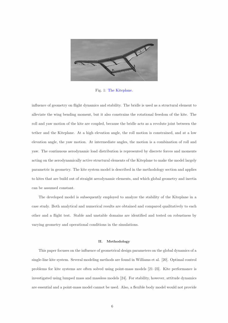
Fig. 1: The Kiteplane.
influence of geometry on flight dynamics and stability. The bridle is used as a structural element to
alleviate the wing bending moment, but it also constrains the rotational freedom of the kite. The
roll and yaw motion of the kite are coupled, because the bridle acts as a revolute joint between the
tether and the Kiteplane. At a high elevation angle, the roll motion is constrained, and at a low
elevation angle, the yaw motion. At intermediate angles, the motion is a combination of roll and
yaw. The continuous aerodynamic load distribution is represented by discrete forces and moments
acting on the aerodynamically active structural elements of the Kiteplane to make the model largely
parametric in geometry. The kite system model is described in the methodology section and applies
to kites that are build out of straight aerodynamic elements, and which global geometry and inertia
can be assumed constant.
The developed model is subsequently employed to analyze the stability of the Kiteplane in a
case study. Both analytical and numerical results are obtained and compared qualitatively to each
other and a flight test. Stable and unstable domains are identified and tested on robustness by
varying geometry and operational conditions in the simulations.
II. Methodology
This paper focuses on the influence of geometrical design parameters on the global dynamics of a
single-line kite system. Several modeling methods are found in Williams et al. [20]. Optimal control
problems for kite systems are often solved using point-mass models [21–23]. Kite performance is
investigated using lumped mass and massless models [24]. For stability, however, attitude dynamics
are essential and a point-mass model cannot be used. Also, a flexible body model would not provide
6
pure geometry-stability relations. Given this scope and the philosophy that the best model is the
smallest model that describes the behavior of interest, a rigid body approach is selected to model
the kite.
Moreover, to investigate the impact of geometry changes on stability, a parametric approach is
required for the aerodynamic forces. To this end, an aerodynamic element discretization is developed
similar to Meijaard et al. [25].
The equations of motion are derived using Lagrange’s equation of the second kind [26], a method
used frequently for the constrained kite systems [27–29].
A. Kite system definition
The kite system consists of a ground station, a tether and a kite. The ground station is
represented by a point object that acts as a forced sink and source of tether length, where the
tether is modeled as a one-dimensional massless rigid rod element that is free to rotate about its
longitudinal axis. As stated before, the kite is modeled as a rigid body.
The 5 Degrees of Freedom (DOF) of the kite system result from the spherical joint between the
ground station and the tether providing 3 rotational DOF, the variable length of the tether and
the revolute joint between the tether and the kite. The bridle connection between the tether and
the kite constrains the freedom of the kite with respect to the tether and couples the roll and yaw
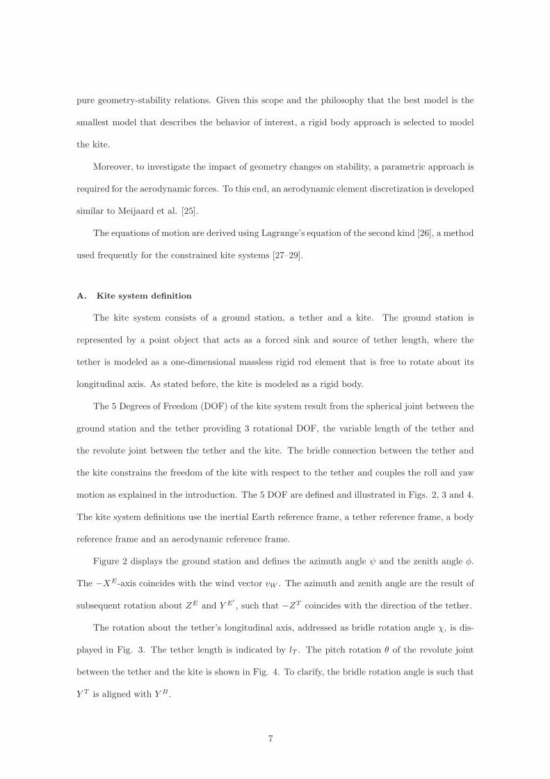
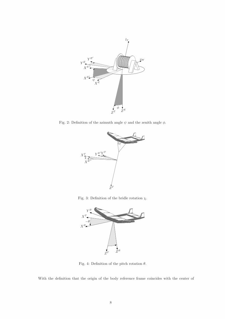
motion as explained in the introduction. The 5 DOF are defined and illustrated in Figs. 2, 3 and 4.
The kite system definitions use the inertial Earth reference frame, a tether reference frame, a body
reference frame and an aerodynamic reference frame.
Figure 2 displays the ground station and defines the azimuth angle ψ and the zenith angle φ.
The −XE-axis coincides with the wind vector vW . The azimuth and zenith angle are the result of
subsequent rotation about ZE and Y E′
, such that −ZT coincides with the direction of the tether.
The rotation about the tether’s longitudinal axis, addressed as bridle rotation angle χ, is dis-
played in Fig. 3. The tether length is indicated by lT . The pitch rotation θ of the revolute joint
between the tether and the kite is shown in Fig. 4. To clarify, the bridle rotation angle is such that
Y T is aligned with Y B.
7
vW
lT
ψ
φ
XE
Y E
ZE
ZT
XE′
XE′′
Y E′
Fig. 2: Definition of the azimuth angle ψ and the zenith angle φ.
lT
χ
XE′′
Y E′
XT Y T
ZT
Fig. 3: Definition of the bridle rotation χ.
XT
ZT
XB
Y B
ZB
−θ
Fig. 4: Definition of the pitch rotation θ.
With the definition that the origin of the body reference frame coincides with the center of
8

gravity (cg), the location of the cg in the Earth reference frame can be expressed as:
rEcg = TET
[
0 0 −lT
]T
+ TEB
[
−xT 0 −zT
]T
. (1)
The coordinates xT and zT represent the location of the bridle hinge line with respect to the
cg, thus to go from the bridle hinge line to the cg they must be subtracted. Expressions for the
rotation matrices TET and TEB are constructed from the angle definitions in Figs. 2, 3 and 4.
The aerodynamic reference frame in Fig. 5 is established from the definition that Xa coincides
with the apparent velocity vector of the kite through subsequent rotations α about Y B and β about
Za. The magnitude of the apparent velocity vector vapp, the angle of attack α, the sideslip angle
β, and the body angular velocity ωcg together determine the aerodynamic forces and moments on
the kite.
vapp
β
αXa
Y a
Za
XB
XB′
Y B
ZB
Fig. 5: Definition of the aerodynamic reference frame.
B. Equations of motion
Lagrange’s equation of the second kind, Eq. (2), is used to derive five second order differential
equations that describe the motion of the kite system.
d
dt
∂T
∂qi−∂T
∂qi+∂V
∂qi= Qi, i = 1, . . . , 5 (2)
The five DOF are represented by the generalized coordinates qi. To evaluate Eq. (2), expressions
need to be found for the kinetic energy T , the potential energy V , and the generalized forces Qi.
9
The kinetic energy is obtained from Eq. (3) by substituting Eq. (4) for vcg and Eq. (6) for ωcg.
T =1
2mkvcg · vcg +
1
2ω
Tcg · I · ωcg (3)
Equation (4) is found by differentiating rcg with respect to time and Eqs. (5) and (6) are
constructed from the definitions in Section IIA.
vTcg =
[
0 0 ˙−lT
]T
+ ωTET
×
[
0 0 −lT
]T
+TTB · ωBEB
×
[
−xT 0 −zT
]T
(4)
ωTET
=
0
0
χ
+ TTE′′
0
φ
0
+ TTE′
0
0
ψ
(5)
ωBEB
=
0
θ
0
+ TBT
0
0
χ
+ TBE′′
0
φ
0
+ TBE′
0
0
ψ
(6)
The potential energy is given by Eq. (7), where mg represents the kite mass excluding the
confined air. To avoid inclusion of buoyancy forces, the confined air mass is subtracted from mk
assuming that the centers of mass coincide.
V = mgg · rcg (7)
Since the kite system is subjected to nonconservative forces such as aerodynamic and ground
station loads, expressions for these forces are required in the form of generalized forces. For a rigid
body, the resulting aerodynamic loads can be expressed as a force vector and a moment vector that
act on the kite cg. In the body reference frame, these two vectors are denoted by respectively FBa
and MBa . The force of the ground station acting on the tether is represented by FTGS in the tether
reference frame.
10

With the nonconservative forces specified, the generalized force Qi for generalized coordinate
qi can be derived using the principle of virtual work in Eq. (8).
Qi =∂r
∂qi·F+
∂ω
∂qi·M, i = 1, . . . , 5 (8)
The results of applying Eqs. (8) to the generalized coordinates in the kite system are displayed
in Eqs. (9) through (13). Note that the nonconservative forces are transformed to the reference
frames corresponding to the generalized coordinates.
Qθ =∂
∂θ
MBa ·
0
θ
0
+ FBa ·
0
θ
0
×
−xT
0
−zT
(9)
Qχ =∂
∂χ
MTa ·
0
0
χ
+ FTa ·
0
0
χ
×
−xT
0
−zT
(10)
QlT =∂
∂lT
(
FTa + FTGS)
·
0
0
−lT
(11)
Qφ =∂
∂φ
ME′′
a ·
0
φ
0
+ FE′′
a ·
0
φ
0
× rE′′
cg
(12)
Qψ =∂
∂ψ
ME′
a ·
0
0
ψ
+ FE′
a ·
0
0
ψ
× rE′
cg
(13)
C. Aerodynamic model
In the generalized forces, the aerodynamics are incorporated through the force vector Fa and
moment vector Ma. However, an expression for these vectors is yet to be found. For this purpose,
11
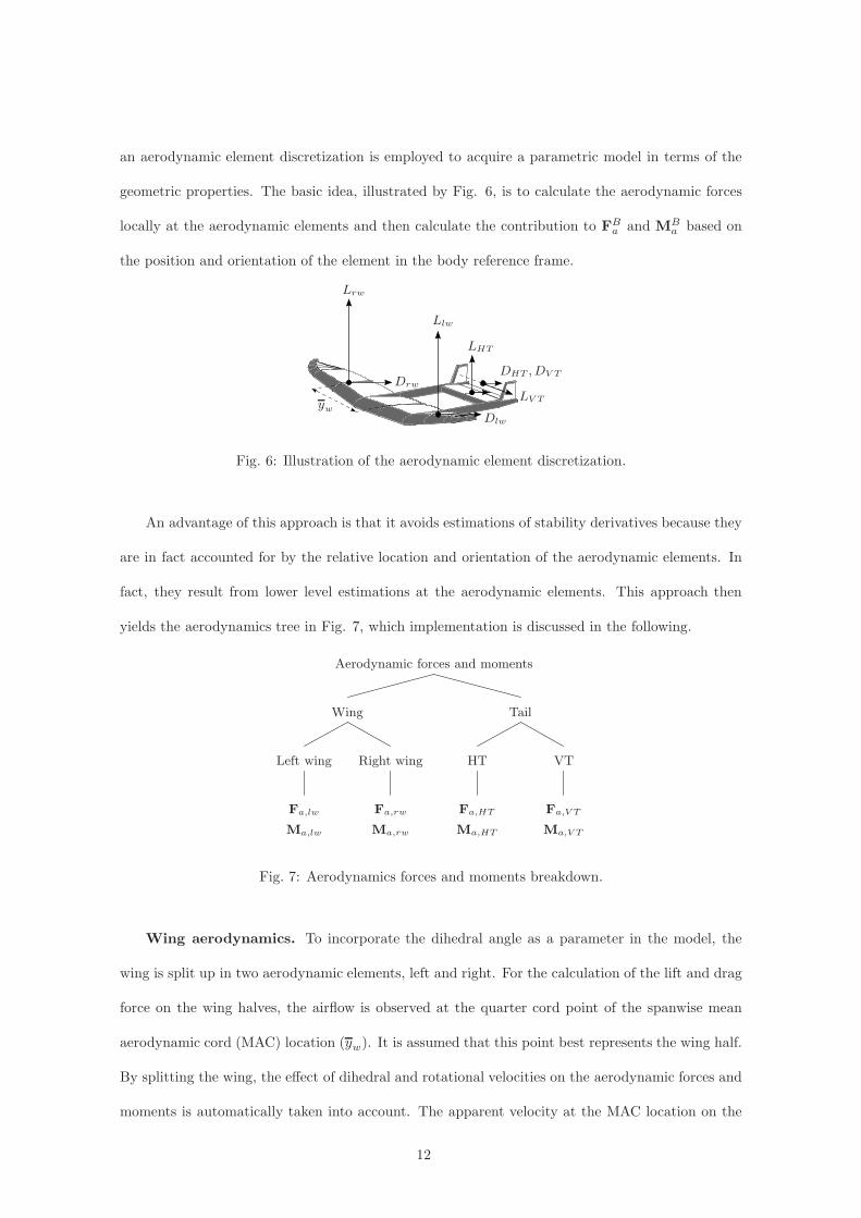
an aerodynamic element discretization is employed to acquire a parametric model in terms of the
geometric properties. The basic idea, illustrated by Fig. 6, is to calculate the aerodynamic forces
locally at the aerodynamic elements and then calculate the contribution to FBa and MBa based on
the position and orientation of the element in the body reference frame.
LHT
LV T
DHT , DV TDrw
Dlw
yw
Llw
Lrw
Fig. 6: Illustration of the aerodynamic element discretization.
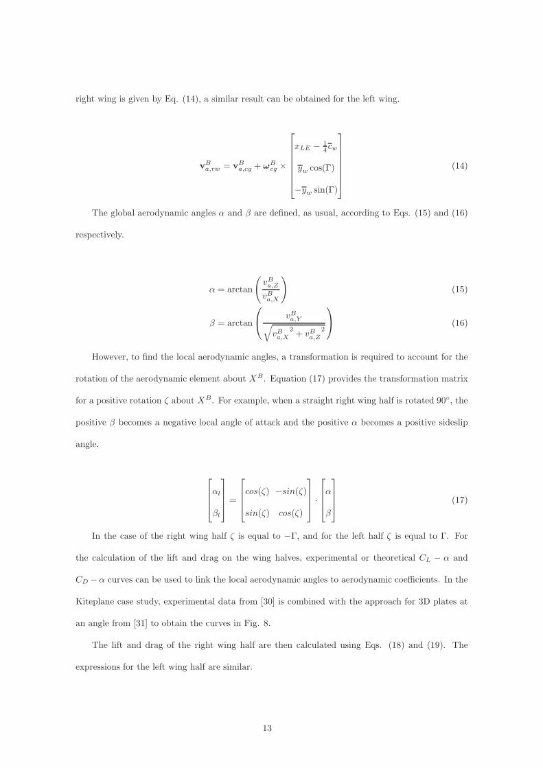
An advantage of this approach is that it avoids estimations of stability derivatives because they
are in fact accounted for by the relative location and orientation of the aerodynamic elements. In
fact, they result from lower level estimations at the aerodynamic elements. This approach then
yields the aerodynamics tree in Fig. 7, which implementation is discussed in the following.
Aerodynamic forces and moments
Wing Tail
Left wing Right wing HT VT
Fa,lw
Ma,lw
Fa,rw
Ma,rw
Fa,HT
Ma,HT
Fa,V T
Ma,V T
Fig. 7: Aerodynamics forces and moments breakdown.
Wing aerodynamics. To incorporate the dihedral angle as a parameter in the model, the
wing is split up in two aerodynamic elements, left and right. For the calculation of the lift and drag
force on the wing halves, the airflow is observed at the quarter cord point of the spanwise mean
aerodynamic cord (MAC) location (yw). It is assumed that this point best represents the wing half.
By splitting the wing, the effect of dihedral and rotational velocities on the aerodynamic forces and
moments is automatically taken into account. The apparent velocity at the MAC location on the
12
right wing is given by Eq. (14), a similar result can be obtained for the left wing.
vBa,rw = vBa,cg + ωBcg ×
xLE −1
4cw
yw cos(Γ)
−yw sin(Γ)
(14)
The global aerodynamic angles α and β are defined, as usual, according to Eqs. (15) and (16)
respectively.
α = arctan
(
vBa,ZvBa,X
)
(15)
β = arctan
vBa,Y√
vBa,X2+ vBa,Z
2
(16)
However, to find the local aerodynamic angles, a transformation is required to account for the
rotation of the aerodynamic element about XB. Equation (17) provides the transformation matrix
for a positive rotation ζ about XB. For example, when a straight right wing half is rotated 90◦, the
positive β becomes a negative local angle of attack and the positive α becomes a positive sideslip
angle.
αl
βl
=
cos(ζ) −sin(ζ)
sin(ζ) cos(ζ)
·
α
β
(17)
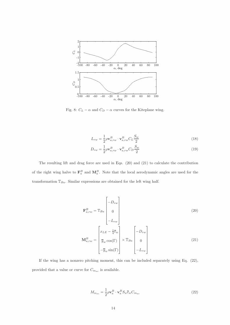
In the case of the right wing half ζ is equal to −Γ, and for the left half ζ is equal to Γ. For
the calculation of the lift and drag on the wing halves, experimental or theoretical CL − α and
CD −α curves can be used to link the local aerodynamic angles to aerodynamic coefficients. In the
Kiteplane case study, experimental data from [30] is combined with the approach for 3D plates at
an angle from [31] to obtain the curves in Fig. 8.
The lift and drag of the right wing half are then calculated using Eqs. (18) and (19). The
expressions for the left wing half are similar.
13
CL
α, deg
CD
α, deg-100 -80 -60 -40 -20 0 20 40 60 80 100
-100 -80 -60 -40 -20 0 20 40 60 80 100
0
0.5
1
1.5
-2
-1
0
1
2
Fig. 8: CL − α and CD − α curves for the Kiteplane wing.
Lrw =1
2ρvBa,rw · vBa,rwCL
Sw2
(18)
Drw =1
2ρvBa,rw · vBa,rwCD
Sw2
(19)
The resulting lift and drag force are used in Eqs. (20) and (21) to calculate the contribution
of the right wing halve to FBa and MBa . Note that the local aerodynamic angles are used for the
transformation TBa. Similar expressions are obtained for the left wing half.
FBa,rw = TBa
−Drw
0
−Lrw
(20)
MBa,rw =
xLE − 1
4cw
yw cos(Γ)
−yw sin(Γ)
× TBa
−Drw
0
−Lrw
(21)
If the wing has a nonzero pitching moment, this can be included separately using Eq. (22),
provided that a value or curve for Cmacis available.
Mwac=
1
2ρvBa · vBa SwcwCmac
(22)
14
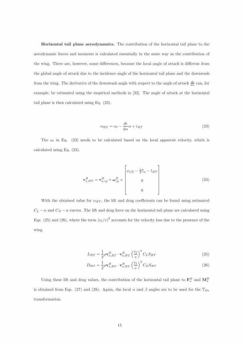
Horizontal tail plane aerodynamics. The contribution of the horizontal tail plane to the
aerodynamic forces and moments is calculated essentially in the same way as the contribution of
the wing. There are, however, some differences, because the local angle of attack is different from
the global angle of attack due to the incidence angle of the horizontal tail plane and the downwash
from the wing. The derivative of the downwash angle with respect to the angle of attack dεdα
can, for
example, be estimated using the empirical methods in [32]. The angle of attack at the horizontal
tail plane is then calculated using Eq. (23).
αHT = αl −dε
dαα+ iHT (23)
The αl in Eq. (23) needs to be calculated based on the local apparent velocity, which is
calculated using Eq. (24).
vBa,HT = vBa,cg + ωBcg ×
xLE −1
4cw − lHT
0
0
(24)
With the obtained value for αHT , the lift and drag coefficients can be found using estimated
CL−α and CD −α curves. The lift and drag force on the horizontal tail plane are calculated using
Eqs. (25) and (26), where the term (vt/v)2 accounts for the velocity loss due to the presence of the
wing.
LHT =1
2ρvBa,HT · vBa,HT
(vtv
)2
CLSHT (25)
DHT =1
2ρvBa,HT · vBa,HT
(vtv
)2
CDSHT (26)
Using these lift and drag values, the contribution of the horizontal tail plane to FBa and MBa
is obtained from Eqs. (27) and (28). Again, the local α and β angles are to be used for the TBa
transformation.
15

FBa,HT = TBa
−DHT
0
−LHT
(27)
MBa,HT =
xLE − 1
4cw − lHT
0
0
× TBa
−DHT
0
−LHT
(28)
Vertical tail plane aerodynamics. As with the other elements, a single resultant force is
calculated at the quarter cord point of the spanwise MAC location. In the Kiteplane case study
there are in fact two vertical fins, which are approximated by a single element using the fins original
MAC location and aerodynamics properties, but taking into account twice the size. Due to the
simplifications in the model, this is equal to including both fins separately when the small effect of
the lateral position of the fins on the distance to the equivalent vertical tail plane is neglected. The
local velocity at the vertical tail plane is given by Eq. (29).
vBa,V T = vBa,cg + ωBcg ×
xLE −1
4cV T − lV T
0
zLE − zV T
(29)
Since the vertical tail plane element is rotated -90◦ about the XB-axis, the angle of attack for
the vertical tail plane is equal to the sideslip angle resulting from Eq. (16).
With αV T determined, the lift and drag coefficients can again be obtained from estimated CL−α
and CD − α curves. The lift and drag force on the vertical tail plane are calculated with equations
similar to Eqs. (25) and (26), and inserted in Eqs. (30) and (31) to find the contribution to FBa
and MBa .
16

FBa,V T = TBa
−DV T
−LV T
0
(30)
MBa,V T =
xLE − 1
4cw − lV T
0
zLE − zV T
× TBa
−DHT
−LHT
0
(31)
D. Ground station force
Since the tether is modeled as a massless rigid one-dimensional rod, the ground station accounts
for the spring damper dynamics. This approach combines the tether dynamics and ground station
dynamics in a single force. The ground station force that represents the spring damper dynamics of
a fixed length tether is given by Eq. (32), where k represents the spring constant and d the damping
constant. Both properties depend on the tether material, thickness and length.
FGS =
k (lT − lT0) + dlT , lT ≥ lT0
0, lT < lT0
(32)
III. Results of the Kiteplane case study
With the described methodology, analytical as well as numerical results can be obtained for
various aircraft shaped kites. In this paper a case study is preformed on a specific kite, the Kiteplane,
to investigate whether the developed model can describe its dominating behavior. The Kiteplane,
displayed in previous figures, features an approximate elliptic wing with positive dihedral from the
tail boom section to the tips and is in size comparable to a small surfkite. The twin tail booms
support the horizontal tail plane that is located in between and the two vertical tail planes on
top. The main geometrical properties are listed in Table 1, where the MAC and its location are
calculated using the definitions from [33].
The inertia of the Kiteplane consists of three parts: the pressurized beam structure, the canopy
surfaces, and the air confined in the tubes and airfoils. The contribution of displaced air is assumed
17

Table 1: Geometric properties of the Kiteplane.
Component Parameter Symbol Value Unit
Wing Surface area Sw 5.67 m2
Aspect ratio Aw 5.65
Taper ratio λ 0.66
Dihedral angle1 Γ 14 Deg
MAC cw 1.08 m
MAC location yw 1.21 m
Airframe Total length l 3.08 m
HT distance lHT 2.24 m
VT distance lV T 2.56 m
HT Surface area SHT 1.28 m2
Aspect ratio AHT 2.2
MAC cHT 0.76 m
VT 2 × surface area SV T 0.33 m2
Aspect ratio AV T 1.2
Taper ratio λV T 0.59
LE sweep ΛLE,V T 23 Deg
MAC cV T 0.38 m
MAC location yV T 0.20 m
1 Of the outer wing.
to be negligible, because the Kiteplane is still about five times heavier than air. Estimations based
on the CAD model give the following properties:
18
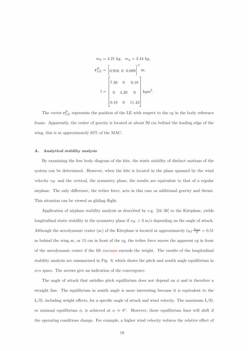
mk = 4.21 kg, mg = 3.44 kg,
rBLE =
[
0.916 0 0.089
]T
m,
I =
7.38 0 0.18
0 4.20 0
0.18 0 11.43
kgm2.
The vector rBLE represents the position of the LE with respect to the cg in the body reference
frame. Apparently, the center of gravity is located at about 92 cm behind the leading edge of the
wing, this is at approximately 85% of the MAC.
A. Analytical stability analysis
By examining the free body diagram of the kite, the static stability of distinct motions of the
system can be determined. However, when the kite is located in the plane spanned by the wind
velocity vW and the vertical, the symmetry plane, the results are equivalent to that of a regular
airplane. The only difference, the tether force, acts in this case as additional gravity and thrust.
This situation can be viewed as gliding flight.
Application of airplane stability analysis as described by e.g. [34–36] to the Kiteplane, yields
longitudinal static stability in the symmetry plane if vW > 3 m/s depending on the angle of attack.
Although the aerodynamic center (ac) of the Kiteplane is located at approximately lHTSHT
S= 0.51
m behind the wing ac, or 15 cm in front of the cg, the tether force moves the apparent cg in front
of the aerodynamic center if the lift excesses exceeds the weight. The results of the longitudinal
stability analysis are summarized in Fig. 9, which shows the pitch and zenith angle equilibrium in
φ-α space. The arrows give an indication of the convergence.
The angle of attack that satisfies pitch equilibrium does not depend on φ and is therefore a
straight line. The equilibrium in zenith angle is more interesting because it is equivalent to the
L/D, including weight effects, for a specific angle of attack and wind velocity. The maximum L/D,
or minimal equilibrium φ, is achieved at α ≈ 8◦. However, these equilibrium lines will shift if
the operating conditions change. For example, a higher wind velocity reduces the relative effect of
19
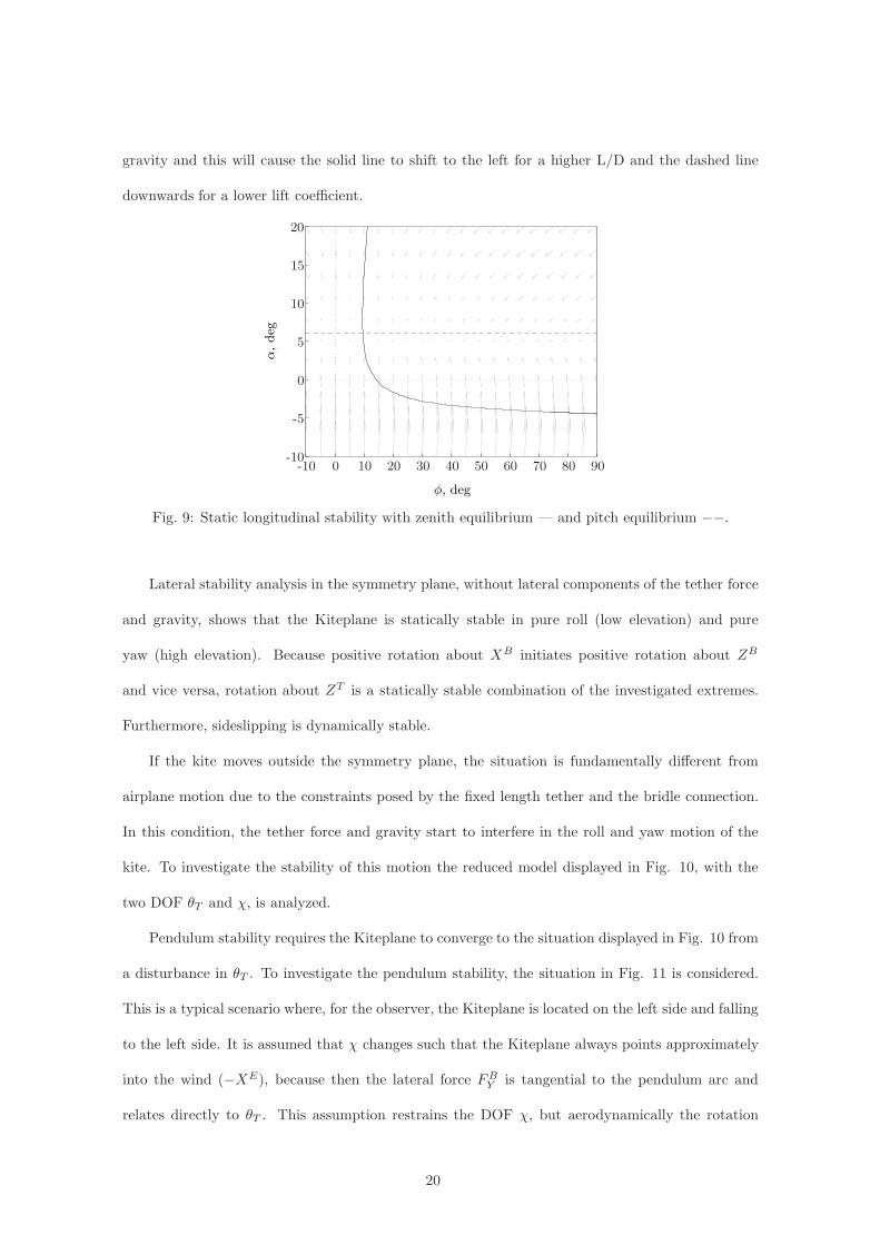
gravity and this will cause the solid line to shift to the left for a higher L/D and the dashed line
downwards for a lower lift coefficient.
φ, deg
α,deg
-10 0 10 20 30 40 50 60 70 80 90-10
-5
0
5
10
15
20
Fig. 9: Static longitudinal stability with zenith equilibrium — and pitch equilibrium −−.
Lateral stability analysis in the symmetry plane, without lateral components of the tether force
and gravity, shows that the Kiteplane is statically stable in pure roll (low elevation) and pure
yaw (high elevation). Because positive rotation about XB initiates positive rotation about ZB
and vice versa, rotation about ZT is a statically stable combination of the investigated extremes.
Furthermore, sideslipping is dynamically stable.
If the kite moves outside the symmetry plane, the situation is fundamentally different from
airplane motion due to the constraints posed by the fixed length tether and the bridle connection.
In this condition, the tether force and gravity start to interfere in the roll and yaw motion of the
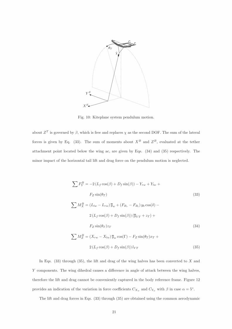
kite. To investigate the stability of this motion the reduced model displayed in Fig. 10, with the
two DOF θT and χ, is analyzed.
Pendulum stability requires the Kiteplane to converge to the situation displayed in Fig. 10 from
a disturbance in θT . To investigate the pendulum stability, the situation in Fig. 11 is considered.
This is a typical scenario where, for the observer, the Kiteplane is located on the left side and falling
to the left side. It is assumed that χ changes such that the Kiteplane always points approximately
into the wind (−XE), because then the lateral force FBY is tangential to the pendulum arc and
relates directly to θT . This assumption restrains the DOF χ, but aerodynamically the rotation
20
χ
θT
XE
Y E
Fig. 10: Kiteplane system pendulum motion.
about ZT is governed by β, which is free and replaces χ as the second DOF. The sum of the lateral
forces is given by Eq. (33). The sum of moments about XB and ZB, evaluated at the tether
attachment point located below the wing ac, are given by Eqs. (34) and (35) respectively. The
minor impact of the horizontal tail lift and drag force on the pendulum motion is neglected.
∑
FBY = −2 (Lf cos(β) +Df sin(β))− Yrw + Ylw +
FZ sin(θT ) (33)
∑
MBX = (Llw − Lrw) yw + (FBr
− FBl) yb cos(δ)−
2 (Lf cos(β) +Df sin(β)) (yV T + zT ) +
FZ sin(θT )zT (34)
∑
MBZ = (Xrw −Xlw) yw cos(Γ)− FZ sin(θT )xT +
2 (Lf cos(β) +Df sin(β)) lV T (35)
In Eqs. (33) through (35), the lift and drag of the wing halves has been converted to X and
Y components. The wing dihedral causes a difference in angle of attack between the wing halves,
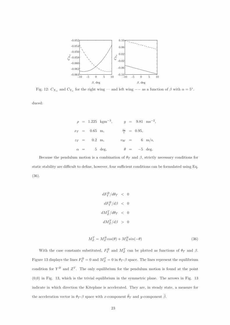
therefore the lift and drag cannot be conveniently captured in the body reference frame. Figure 12
provides an indication of the variation in force coefficients CXwand CYw
with β in case α = 5◦.
The lift and drag forces in Eqs. (33) through (35) are obtained using the common aerodynamic
21

vapp
δ
FZ
β
θT
XE
Y E
XlwXrw
Ylw Yrw
Llw
Lrw
LfLf
DfDf
FBlFBr
Fig. 11: Front and top view of the Kiteplane in pendulum motion.
relations in Section II C. The forces like Xrw are calculated similarly, but now the drag coefficient
is for example replaced by CXrw. Note that these forces are simply transformations of lift and drag.
The gravitational force FZ is found by multiplying mg with the gravitational acceleration.
To find quantitative results for the pendulum stability, the following case constants are intro-
22
β, deg
CX
w
β, deg
CYw
-10 -5 0 5 10-10 -5 0 5 10-0.10
-0.06
-0.02
0.02
0.06
0.10
-0.064
-0.062
-0.060
-0.058
-0.056
-0.054
-0.052
Fig. 12: CXwand CYw
for the right wing — and left wing −− as a function of β with α = 5◦.
duced:
ρ = 1.225 kgm−3, g = 9.81 ms−2,
xT = 0.65 m, vtv
= 0.95,
zT = 0.2 m, vW = 6 m/s,
α = 5 deg, θ = −5 deg.
Because the pendulum motion is a combination of θT and β, strictly necessary conditions for
static stability are difficult to define, however, four sufficient conditions can be formulated using Eq.
(36).
dFBY /dθT < 0
dFBY /dβ < 0
dMTZ /dθT < 0
dMTZ /dβ > 0
MTZ =MB
Z cos(θ) +MBXsin(−θ) (36)
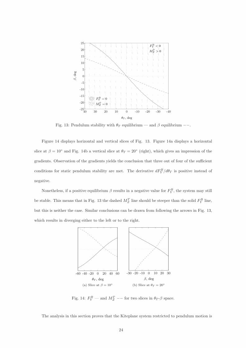
With the case constants substituted, FBY and MTZ can be plotted as functions of θT and β.
Figure 13 displays the lines FBY = 0 and MTZ = 0 in θT -β space. The lines represent the equilibrium
condition for Y B and ZT . The only equilibrium for the pendulum motion is found at the point
(0,0) in Fig. 13, which is the trivial equilibrium in the symmetric plane. The arrows in Fig. 13
indicate in which direction the Kiteplane is accelerated. They are, in steady state, a measure for
the acceleration vector in θT -β space with x-component θT and y-component β.
23
θT , deg
β,deg
FBY < 0
MTZ > 0
FBY = 0
MTZ = 0
-40-30-20-10010203040-25
-20
-15
-10
-5
0
5
10
15
20
25
Fig. 13: Pendulum stability with θT equilibrium — and β equilibrium −−.
Figure 14 displays horizontal and vertical slices of Fig. 13. Figure 14a displays a horizontal
slice at β = 10◦ and Fig. 14b a vertical slice at θT = 20◦ (right), which gives an impression of the
gradients. Observation of the gradients yields the conclusion that three out of four of the sufficient
conditions for static pendulum stability are met. The derivative dFBY /dθT is positive instead of
negative.
Nonetheless, if a positive equilibrium β results in a negative value for FBY , the system may still
be stable. This means that in Fig. 13 the dashed MTZ line should be steeper than the solid FBY line,
but this is neither the case. Similar conclusions can be drawn from following the arrows in Fig. 13,
which results in diverging either to the left or to the right.
θT , deg
-60 -40 -20 0 20 40 60
(a) Slice at β = 10◦
β, deg
-30 -20 -10 0 10 20 30
(b) Slice at θT = 20◦
Fig. 14: FBY — and MTZ −− for two slices in θT -β space.
The analysis in this section proves that the Kiteplane system restricted to pendulum motion is
24
unstable. This cannot be guaranteed for the unrestricted Kiteplane system, but it is nevertheless
likely that it exhibits some of this unstable behavior. The investigation of this pendulum motion is
continued trough numerical simulation.
B. Numerical simulation results
To study the motion of the Kiteplane, numerical simulations are produced with a MAT-
LAB/Simulink model that is constructed from the derived equations of motion. The model is
used to solve initial value problems, which results can subsequently be compared to other simula-
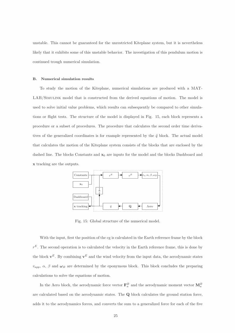
tions or flight tests. The structure of the model is displayed in Fig. 15, each block represents a
procedure or a subset of procedures. The procedure that calculates the second order time deriva-
tives of the generalized coordinates is for example represented by the q block. The actual model
that calculates the motion of the Kiteplane system consists of the blocks that are enclosed by the
dashed line. The blocks Constants and x0 are inputs for the model and the blocks Dashboard and
x tracking are the outputs.
Constants
Aerox tracking
Dashboard
rE vE va, α, β, ωB
1
s
x0
Fig. 15: Global structure of the numerical model.
With the input, first the position of the cg is calculated in the Earth reference frame by the block
rE . The second operation is to calculated the velocity in the Earth reference frame, this is done by
the block vE . By combining vE and the wind velocity from the input data, the aerodynamic states
vapp, α, β and ωB are determined by the eponymous block. This block concludes the preparing
calculations to solve the equations of motion.
In the Aero block, the aerodynamic force vector FBa and the aerodynamic moment vector MBa
are calculated based on the aerodynamic states. The Q block calculates the ground station force,
adds it to the aerodynamics forces, and converts the sum to a generalized force for each of the five
25
generalized coordinates. The second derivatives of the generalized coordinates are calculated by the
q block. The 1
sblock concludes the time step by integrating the state vector derivative to find the
new state. After this, the whole procedure is repeated until the time reaches the predefined end
time of the simulation.
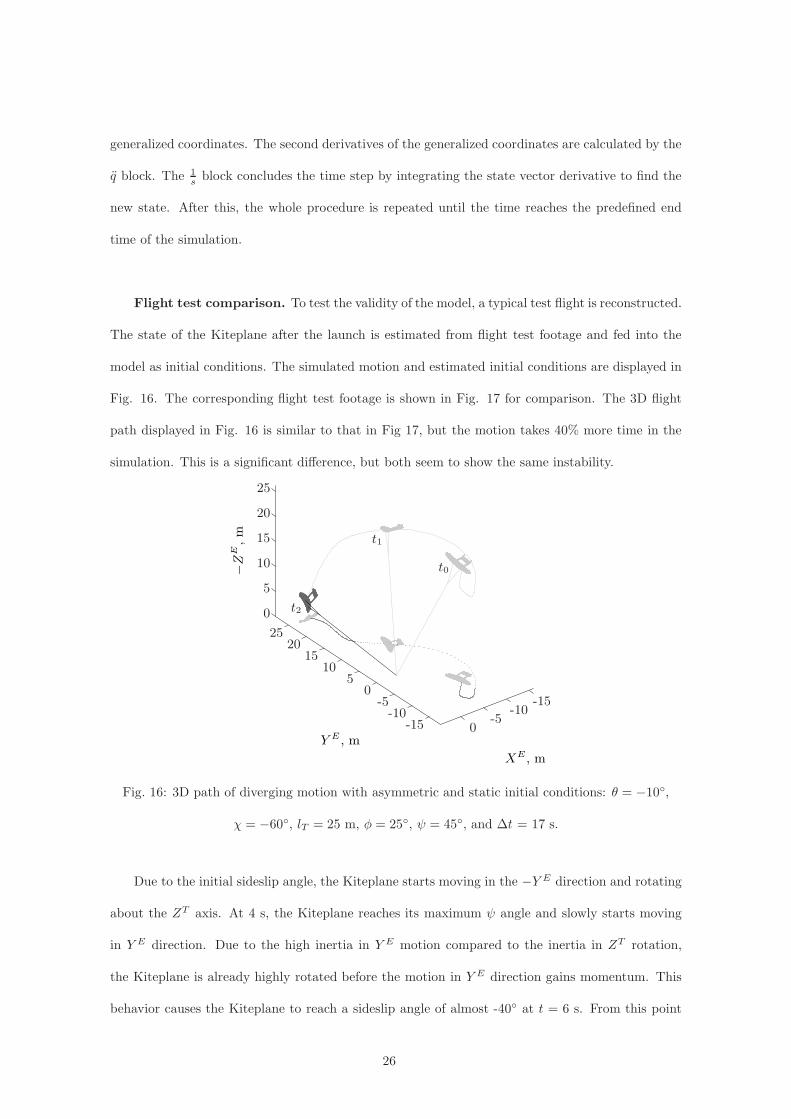
Flight test comparison. To test the validity of the model, a typical test flight is reconstructed.
The state of the Kiteplane after the launch is estimated from flight test footage and fed into the
model as initial conditions. The simulated motion and estimated initial conditions are displayed in
Fig. 16. The corresponding flight test footage is shown in Fig. 17 for comparison. The 3D flight
path displayed in Fig. 16 is similar to that in Fig 17, but the motion takes 40% more time in the
simulation. This is a significant difference, but both seem to show the same instability.
XE , m
Y E , m
−Z
E,m
t0
t1
t2
-15-10
-50-15
-10-5
05
1015
2025
0
5
10
15
20
25
Fig. 16: 3D path of diverging motion with asymmetric and static initial conditions: θ = −10◦,
χ = −60◦, lT = 25 m, φ = 25◦, ψ = 45◦, and ∆t = 17 s.
Due to the initial sideslip angle, the Kiteplane starts moving in the −Y E direction and rotating
about the ZT axis. At 4 s, the Kiteplane reaches its maximum ψ angle and slowly starts moving
in Y E direction. Due to the high inertia in Y E motion compared to the inertia in ZT rotation,
the Kiteplane is already highly rotated before the motion in Y E direction gains momentum. This
behavior causes the Kiteplane to reach a sideslip angle of almost -40◦ at t = 6 s. From this point
26

Fig. 17: Composite photo constructed from flight test footage with vW ≈ 6 ms−1, the flight time
captured in this figure is approximately 12 s.
on, the Kiteplane starts accelerating in Y E direction with increasing α, increasing vapp and quickly
reducing β. At the passing of −XE, the same inertia that initially kept the Kiteplane from returning
to ψ = 0 is now causing a major overshoot in ψ. At about 11 s, the Kiteplane is pushed toward a
point of no return and falls to the ground. The increase in β at this point is insufficient to generate
a large enough aerodynamic force in −Y B direction to overcome the gravity component in Y B
direction.
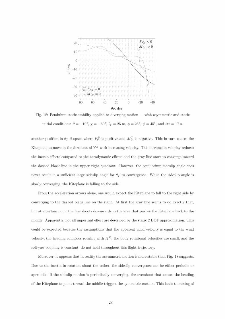
The pendulum motion that was studied analytically in the previous section seems dominant
in this flight and it appears that the analytical approach as well as the simulation agree on the
instability that is observed in reality. A comparison of the simulation and the analytical pendulum
analysis is displayed in Fig. 18. The simulated trajectory in θT -β space is indicated by the gray
line, with the circle mark as starting point and the cross mark as final state.
As explained previously, a position above and to the right of the solid and dashed black lines
yields respectively a negative force in Y B and a positive moment about ZT . Similarly, a position
below and to the left of the solid and dashed black lines yields respectively a positive force in Y B
and a negative moment about ZT . The magnitude of the force and moment increases with distance
from the equilibrium lines. The arrows show approximately the local acceleration vector in θT -β
space and are therefore the most intuitive means to determine the expected direction of motion.
Thus, in the starting condition, FBY is negative and MTZ is positive. This is in correspondence
with the motion displayed in Fig. 16. Subsequently, this motion causes the Kiteplane to move to
27
θT , deg
β,deg
FYB< 0
MZT> 0
FYB= 0
MZT= 0
-40-20020406080
-40
-30
-20
-10
0
10
20
Fig. 18: Pendulum static stability applied to diverging motion — with asymmetric and static
initial conditions: θ = −10◦, χ = −60◦, lT = 25 m, φ = 25◦, ψ = 45◦, and ∆t = 17 s.
another position in θT -β space where FBY is positive and MTZ is negative. This in turn causes the
Kiteplane to move in the direction of Y E with increasing velocity. This increase in velocity reduces
the inertia effects compared to the aerodynamic effects and the gray line start to converge toward
the dashed black line in the upper right quadrant. However, the equilibrium sideslip angle does
never result in a sufficient large sideslip angle for θT to convergence. While the sideslip angle is
slowly converging, the Kiteplane is falling to the side.
From the acceleration arrows alone, one would expect the Kiteplane to fall to the right side by
converging to the dashed black line on the right. At first the gray line seems to do exactly that,
but at a certain point the line shoots downwards in the area that pushes the Kiteplane back to the
middle. Apparently, not all important effect are described by the static 2 DOF approximation. This
could be expected because the assumptions that the apparent wind velocity is equal to the wind
velocity, the heading coincides roughly with XE, the body rotational velocities are small, and the
roll-yaw coupling is constant, do not hold throughout this flight trajectory.
Moreover, it appears that in reality the asymmetric motion is more stable than Fig. 18 suggests.
Due to the inertia in rotation about the tether, the sideslip convergence can be either periodic or
aperiodic. If the sideslip motion is periodically converging, the overshoot that causes the heading
of the Kiteplane to point toward the middle triggers the symmetric motion. This leads to mixing of
28

the unstable asymmetric motion with the stable symmetric motion, which increases the apparent
lateral stability.
If the dashed line in Fig. 18 is relatively steep, i.e. sideslip equilibrium is achieved at high
sideslip angles, the Kiteplane tends to rotate more, and this induces the mixing of symmetric and
asymmetric motion. A relatively flat solid line, which it is not in this case, allows more time for
rotation and hence increases apparent lateral stability. In fact, the Kiteplane system can be stable
even when the solid line is slightly steeper than the dashed line.
To summarize, the validity of the static 2 DOF analysis is limited, but it does provide useful
insights in the cause of the instability. It seems essential to have a small enough vertical tail plane
to achieve a large enough equilibrium sideslip angle, and a large enough lateral area to generate a
strong enough lateral force. To test this hypothesis, simulations are run with various vertical tail
plane sizes and dihedral angles.
Impact of design variations on stability. Inspection of Table 1 yields many geometrical
parameters to investigate, but only the ones with the largest impact on the stability are really
interesting for the scope of this paper. The main parameters for longitudinal stability are SHT
Sw
and lHT
c. Since this case study is on the Kiteplane, the wing dimensions are kept constant for
convenience and varying SHT and lHT is therefore equivalent to varying the ratios.
Figure 19 shows the effect of reducing the tail boom length on longitudinal stability. The
trajectory indicated by the gray lines is the launch motion, where the dashed line represents that
for the original size. The effect of reducing SHT by 20% yields similar results. Apparently, the
horizontal tail plane contribution can be reduced without jeopardizing stability, the 20% reduction
even decreases the overshoot in φ significantly.
For the lateral stability, the interesting parameters are SV T , lV T and Γ. Next to these param-
eters, the inclusion of an additional lateral surface on top or below the wing is regarded interesting
as well. The main effect of such a surface can be achieved with dihedral as well, but secondary
effects are inherently different. The most noticeable difference is the effect of dihedral on the yaw
moment, which is absent for a single vertical surface in the middle of the Kiteplane.
29

φ, deg
α,deg
0 20 40 60 80-10
0
10
20
Fig. 19: Effect of 20% reduction in tail boom length on longitudinal stability during launch,
original length −− and reduced length —.
Nevertheless, the parameters SV T and Γ are selected for the lateral stability investigation.
Keeping the tail boom length constant avoids side effects on longitudinal stability and adjusting Γ
is simply found more elegant than the addition of a vertical surface. The impact of variations in
SV T and Γ on the inertia is neglected to keep the results depending on geometry only. The effects
due to changing inertia are investigated at a later stage.
The stability is assessed based on simulation results in the range −10◦ < Γ < 40◦ and 0 <
SV T
SV T0
< 8 for two different wind velocities. The arrangements of the stability domains are displayed
in Fig. 20. Basically, small vertical tail planes cause diverging oscillations and low dihedral angles
cause aperiodic divergence. Stability requires a large dihedral angle and a vertical tail plane of
about 1 to 3 times the original size. Furthermore, the stable domain increases with increasing wind
velocity.
For low dihedral angles and low wind velocities, increasing the vertical tail size leads from
unstable oscillations to aperiodic divergence. If the dihedral angle and wind velocity are large
enough, a stable regime emerges in between. The stable regime itself consists of three domains. The
first, for a small vertical tail plane, is the stable oscillation. The second, for a medium sized vertical
tail plane, is the converging oscillation. For large vertical tail planes and low dihedral angles,
a domain of aperiodic convergence exists. For higher wind velocities the aperiodic convergence
domain increases in size at the cost of the converging oscillation domain.
30

SV T
SV T0
Γ,deg
0 0.1 0.2 0.3 0.4 0.5 0.6 0.7 0.8 0.9 1-10
-5
0
5
10
15
20
25
30
35
40
(a) vW = 6 m/s
SV T
SV T0
Γ,deg
0 0.1 0.2 0.3 0.4 0.5 0.6 0.7 0.8 0.9 1-10
-5
0
5
10
15
20
25
30
35
40
(b) vW = 10 m/s
SV T
SV T0
Γ,deg
0 1 2 3 4 5 6 7 8-10
-5
0
5
10
15
20
25
30
35
40
(c) vW = 6 m/s
SV T
SV T0
Γ,deg
0 1 2 3 4 5 6 7 8-10
-5
0
5
10
15
20
25
30
35
40
(d) vW = 10 m/s
Diverging oscillation
Stable oscillation Converging oscillation
Aperiodic convergence Aperiodic divergence
Fig. 20: Stability chart depending on SV T
SV T0
and Γ for two wind speeds.
At the boundary of diverging oscillation and stable oscillation something peculiar occurs, which
is visible in Figs. 20a and 20b. At a vertical tail plane size slightly too small for stable oscillation,
there seems to be a small band of Γ values that still yield a semi-stable oscillation. When the
vertical tail plane area is reduced sightly from stable oscillation, the stable figure-eight pattern
starts to oscillate itself. This behavior can be compared with the precession of the rotation axis of
a spinning top. For most cases, the crossing of the figure-eight starts to move in Y E direction, one
circle becomes larger than the other and eventually the Kiteplane crashes into the ground.
Another feature that is invisible in Figs. 20c and 20d are the roots of the different stable
domains. These figures reveal that there is always a converging oscillation domain below the stable
oscillation domain, and that the arrangement of the aperiodic convergence domain is depending a
31

lot on wind velocity.
The pendulum stability according to the five stability domains with a sample flight trajectory
are displayed in Fig. 21. The equilibrium lines in Fig. 21 are calibrated to the average conditions
during the trajectory.
θT , deg
β,deg
-40-2002040
-20
-10
0
10
20
(a) Diverging oscillation
θT , deg
β,deg
-40-2002040
-20
-10
0
10
20
(b) Stable oscillation
θT , deg
β,deg
-40-2002040
-20
-10
0
10
20
(c) Converging oscillationθT , deg
β,deg
-40-2002040
-20
-10
0
10
20
(d) Aperiodic convergence
θT , deg
β,deg
-40-2002040
-20
-10
0
10
20
(e) Aperiodic divergence
Fig. 21: Pendulum stability with θT equilibrium — and β equilibrium −− according to the five
different stability domains, including sample trajectories starting at the circle mark.
The first thing to notice is that the differences between the equilibrium lines is small compared to
32
the resulting trajectory. While the behavior and geometry in both unstable domains is significantly
different, the equilibrium lines have a similar slope difference. It appears that, in general, if the
difference between the slope of the solid and dashed line becomes too large, the system becomes
unstable.
The stable oscillation domain displayed in Fig. 21b is the desired stability space according
to the pendulum stability analysis in Section IIIA. The dashed line is steeper than the solid
line, which means that the Kiteplane converges to a sideslip angle that generates a resultant force
toward θT = 0. However, this configuration lacks damping configuration’s lack of damping results
in continued oscillations.
At the border of stable oscillation and converging oscillation, the dashed line is on top of the
solid line. From the 2 DOF pendulum motion point of view, this is the border to unstable behavior.
However, the longitudinal stability improves lateral stability and is in fact crucial in the entire
converging domain.
If the solid line is only slightly steeper than the dashed line, the motion is still oscillatory. If the
difference in slope becomes larger, the oscillations disappear. This is the domain of aperiodic con-
vergence and illustrates the improved apparent lateral stability very clearly, because the acceleration
arrows indicate divergence.
Nevertheless, if the lateral instability becomes too large for the longitudinal stabilization, the
motion diverges as displayed in Fig. 21e. The absolute slope difference in Figs. 21d and 21e are
about equal, but the relative difference is larger because the slopes in Fig. 21e are shallower.
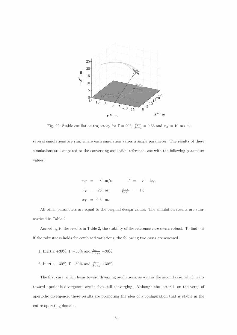
As an additional illustration of the motion of the Kiteplane system, a sample trajectory of stable
oscillation is displayed in Fig. 22. The trajectory starts with a launch from a slight asymmetric
initial condition: χ = −10◦ and ψ = 10◦.
Impact of operating conditions on stability. During kite flight, various operational con-
ditions occur. Also, the presented model is a simplification of reality based on assumptions that
have an impact on accuracy. For these reasons, it is important that stability holds for both varying
conditions and small design variations. To determine the impact of these variations on stability
33
XE , mY E , m
−Z
E,m
-25-20
-15-10
-50-15-10-5051015
0
5
10
15
20
25
Fig. 22: Stable oscillation trajectory for Γ = 20◦, SV T
SV T0
= 0.63 and vW = 10 ms−1.
several simulations are run, where each simulation varies a single parameter. The results of these
simulations are compared to the converging oscillation reference case with the following parameter
values:
vW = 8 m/s, Γ = 20 deg,
lT = 25 m, SV T
SV T0
= 1.5,
xT = 0.3 m.
All other parameters are equal to the original design values. The simulation results are sum-
marized in Table 2.
According to the results in Table 2, the stability of the reference case seems robust. To find out
if the robustness holds for combined variations, the following two cases are assessed.
1. Inertia +30%, Γ +30% and SV T
SV T0
−30%
2. Inertia −30%, Γ −30% and SV T
SV T0
+30%
The first case, which leans toward diverging oscillations, as well as the second case, which leans
toward aperiodic divergence, are in fact still converging. Although the latter is on the verge of
aperiodic divergence, these results are promoting the idea of a configuration that is stable in the
entire operating domain.
34

Table 2: Impact of operating conditions on stability.
Parameter variation Asymmetric initial conditions Lateral step gust of 0.5vW
Reference Converging oscillation Converging oscillation
Inertia−30% More damped oscillation More damped oscillation
+30% Less damped oscillation Less damped oscillation
Γ−30% Aperiodic convergence Aperiodic convergence
+30% Less damped oscillation Less damped oscillation
SV T
SV T0
−30% Less damped oscillation Less damped oscillation
+30% More damped oscillation More damped oscillation
xT
0.0 m More damped oscillation More damped oscillation1
0.55 m Aperiodic convergence Aperiodic convergence
0.6 m Aperiodic divergence Aperiodic divergence
lT
10 m More damped oscillation More damped oscillation
100 m Equal damping, longer period Equal damping, longer period and
lower amplitude
vW
4 ms−1 Less damped oscillation1 Less damped oscillation1
16 ms−1 More damped oscillation1 More damped oscillation1
1 Requires new trim setting for proper longitudinal equilibrium in α.
IV. Conclusions
The geometric requirements for stable flight dynamics of a Kiteplane are different from these
of regular airplanes. Similarities are found in the longitudinal motion, but the constraints resulting
from the tether and the bridle connection give rise to instabilities in the lateral motion outside the
symmetry plane. The pendulum motion in particular poses additional requirements for stability.
With the developed rigid body model, an explanation is found for the pendulum instability of
the Kiteplane design considered in the case study. The analytical analysis yields the hypothesis
that a large wing dihedral angle combined with a small vertical tail plane area provides pendulum
stability. The small vertical tail plane causes the equilibrium sideslip angle to be large enough for
the effective lateral area to generate an aerodynamic force that opposes and overcomes the lateral
component of gravity.
35

Numerical simulations of the derived equations of motion confirm the hypothesis, but the criteria
on the geometry appear to be less strict. Due to the mixing of longitudinal and lateral motion,
stability is achieved with a larger vertical tail plane area than predicted by the analytical results. In
addition, it is found that reducing the horizontal tail plane area by 25 % improves the convergence
of the longitudinal motion.
The numerical simulations are only partially successful in reconstructing the presented test
flight, but this may be improved when more and accurate data becomes available for calibration of
the model.
The results indicate that the stability of the Kiteplane is highly depending on lateral area
parameters. More precisely, the simulation results show that the 2D Kiteplane design space spanned
by dihedral angle and vertical tail plane area consists of the five different stability domains listed
below.
• Unstable oscillation for a dihedral angle > 5◦ and a vertical tail < 3% wing area.
• Stable oscillation for a dihedral angle ∼ 25◦ and a vertical tail ∼ 4.5% wing area.
• Converging oscillation for a dihedral angle ∼ 25◦ and a vertical tail ∼ 9% wing area.
• Aperiodic convergence for a dihedral angle ∼ 25◦ and a vertical tail ∼ 25% wing area.
• Aperiodic divergence for a dihedral angle < 10◦ and a vertical tail > 25% wing area.
In respect to these stability domains, the investigated Kiteplane design features a too small
lateral area that is distributed too far to the back. A geometry change that moves the design to
the converging oscillation domain is, according to the simulation results, stable for a solid range in
design inaccuracies and operational conditions.
ACKNOWLEDGMENTS
The authors are grateful for the financial support provided by the Rotterdam Climate Initiative
and the province of Friesland. They appreciate the cooperation of Lam Sails Ltd. in the production
and the engagement of R. Verheul of the ASSET Institute of Delft University of Technology in the
design, construction and testing of the Kiteplane prototype.
36
REFERENCES
[1] Breukels, J. and Ockels, W. J., “Past, present and future of kites and energy generation,” Power and
Energy Systems Conference 2007 , Clearwater, FL, USA, 3-5 Jan. 2007.
[2] Archer, C. and Caldeira, K., “Global Assessment of High-AltitudeWind Power,”Energies, Vol. 2, No. 2,
2009, pp. 307-319.
doi: 10.3390/en20200307
[3] Rogner, H-H. et al., World Energy Assessment: Energy and the challenge of sustainability , Chapter 5:
Energy Resources, United Nations Development Programme, New York, NY, USA, 2000.
[4] Loyd, L., “Crosswind Kite Power,” Journal of Energy , Vol. 4, No. 3, 1980.
doi: 10.2514/3.48021
[5] Ockels, W. J., “Wind energy converter using kites,” European Patent EP084480, Dutch Patent
NL1004508, Spanish Patent SP2175268, US Patent US6072245, filed Nov. 1996.
[6] Ockels, W. J., “Laddermill, a novel concept to exploit the energy in the airspace,” Journal of Aircraft
Design, Vol. 4, 2001, pp. 81-97.
doi: 10.1016/S1369-8869(01)00002-7
[7] Harvey, M., “The quest to find alternative sources of renewable energy is taking to the skies,” Times
Online, URL: http://business.timesonline.co.uk/ [cited 19 May 2010].
[8] “KitVes Project Funding,” URL: http://www.kitves.com/funding.aspx [cited 19 May 2010].
[9] Botter, M., “Rotterdam ondersteunt Ockels’ project ‘Laddermillship’ met e1 miljoen,” URL:
http://www.obr.rotterdam.nl/smartsite2138537.dws [cited 19 May 2010].
[10] Vance, E., “Wind power: High hopes,”Nature, Vol. 460, 2009, pp. 564-566.
doi: 10.1038/460564a
[11] Canale, M., Fagiano, L., and Milanese, M., “KiteGen: A revolution in wind energy generation,”Energy ,
Vol. 34, 2009, pp. 355-361.
doi: 10.1016/j.energy.2008.10.003
[12] Lansdorp, B. and Ockels, W. J., “Comparison of concepts for high-altitude wind energy generation
with ground based generator,” 2nd China International Renewable Energy Equipment & Technology
Exhibition and Conference, Beijing, China, 25-27 May 2005.
[13] Lansdorp, B. and Ockels, W. J., “Design of a 100 MW laddermill for wind energy generation from 5 km
altitude,” 7th World Congress on Recovery, Recycling and Reintegration, Beijing, China, 25-29 Sept.
2005.
[14] Bryant, L. W., Brown, W. S., and Sweeting, N. E., “Collected Researches on the Stability of Kites and
37
Towed Gliders,” Tech. Rep. 2303, Ministry of Supply, Aeronautical Research Council, London, UK,
1942.
[15] Etkin, B., “Stability of a Towed Body,” Journal of Aircraft , Vol. 35, No. 2, 1998, pp. 197-205.
doi: 10.2514/2.2308
[16] Lambert, C. and Nahon, M., “Stability Analysis of a Tethered Aerostat,” Journal of Aircraft , Vol. 40,
No. 4, 2003, pp. 705-715.
doi: 10.2514/2.3149
[17] Breukels, J., “KitEye,” Faculty of Aerospace Engineering, Delft University of Technology, Delft, The
Netherlands, 2005.
[18] Breukels, J. and Ockels, W. J., “Design of a Large Inflatable Kiteplane,” No. AIAA 2007-2246, 48th
AIAA/ASME/ASCE/AHS/AHC Structures, Structural Dynamics, and Materials Conference, Hon-
olulu, HI, USA, April 2007.
[19] Breukels, J. and Ockels, W. J., “Tethered “kiteplane” design for the Laddermill project,” 4th World
Wind Energy Conference & Renewable Energy Exhibition 2005 , Melbourne, Australia, 2-5 Nov. 2005.
[20] Williams, P., Lansdorp, B., Ruiterkamp, R., and Ockels, W. J., “Modeling, Simulation, and Testing of
Surf Kites for Power Generation,” No. AIAA 2008-6693, AIAA Modeling and Simulation Technologies
Conference and Exhibit , Honolulu, Hi, USA, 18-21 Aug. 2008.
[21] Williams, P., Lansdorp, B., and Ockels, W. J., “Optimal Crosswind Towing and Power Generation with
Tethered Kites,”AIAA Journal of Guidance, Control and Dynamics, Vol. 31, No. 1, 2008, pp. 81-93.
doi: 10.2514/1.30089
[22] Fagiano, L., Control of Tethered Airfoils for High-Altitude Wind Energy Generation, Ph.D. Dissertation,
Royal Turin Polytechnic, Turin, Italy, 2009.
[23] Houska, B. and Diehl, M., “Optimal Control of Towing Kites,” No. ThA10.3, Proceedings of the 45th
IEEE Conference on Decision & Control , San Diego, CA, USA, 13-15 Dec. 2006.
[24] Dadd, G. M., Hudson, D. A., and Shenoi, R. A., “Comparison of Two Kite Force Models with Experi-
ment,” Journal of Aircraft , Vol. 47, No. 1, 2010, pp. 212-224.
doi: 10.2514/1.44738
[25] Meijaard, J. P., Ockels, W. J., and Schwab, A. L., “Modelling of the Dynamic Behaviour of a Laddermill,
A Novel Concept to Exploit Wind Energy,” Proceedings of the 3rd International Symposium on Cable
Dynamics, Trondheim, Norway, 16-18 Aug. 1999, pp. 229-234.
[26] Zatzkis, H., Fundamental formulas of physics, Vol. 1, Section 1.4, Courier Dover, 2nd ed., 1960.
[27] Williams, P., Lansdorp, B., and Ockels, W. J., “Optimal Trajectories for Tethered Kite Mounted
38
on a Vertical Axis Generator,” No. AIAA 2007-6706, AIAA Modeling and Simulation Technologies
Conference and Exhibit , Hilton Head, SC, USA, 20-23 Aug. 2007.
[28] Williams, P., Lansdorp, B., and Ockels, W. J., “Modeling of Optimal Power Generation using Multiple
Kites,” No. AIAA 2008-6691, AIAA Modeling and Simulation Technologies Conference and Exhibit ,
Honolulu, HI, 18-21 Aug. 2008.
[29] Williams, P., Lansdorp, B., and Ockels, W. J., “Flexible Tethered Kite with Moveable Attachment
Points, Part I: Dynamics and Control,” No. AIAA 2007-6628, AIAA Atmospheric Flight Mechanics
Conference and Exhibit , Hilton Head, SC, USA, 20-23 Aug. 2007.
[30] Fink, M. P., “Full-Scale investigation of the aerodynamic characteristics of a sailwing of aspect ra-
tio 5.9,” Tech. Rep. NASA TN D-5047, Langley Research Center, National Aeronautics and Space
Administration, Langley Station, Hampton, VA, USA, 1969.
[31] Hoerner, S. F., Fluid-Dynamic Drag , Hoerner Fluid Dynamics, Vancouver, Canada, 1965.
[32] Hoak, D. E. and Finck, R. D., “The USAF Stability and Control DATCOM,” Tech. Rep. TR-83-3048,
Section 4.4.1, Air Force Wright Aeronautical Laboratories, Wright-Patterson Air Force Base, Fairborn,
OH, USA, 1960.
[33] Torenbeek, E., Synthesis of Subsonic Airplane Design, Appendix A-3.3, Delft University Press, Delft,
The Netherlands, 1982.
[34] Etkin, B., Dynamics of Atmospheric Flight , John Wiley & Sons, Inc, New York, NY, USA, 1972.
[35] Roskam, J., Airplane Flight Dynamics and Automatic Flight Controls, DARcorporation, Lawrence, KS,
USA, 2001.
[36] Mulder, J. A., van Staveren, W. H. J. J., van der Vaart, J. C., and de Weerdt, E., Flight Dynamics,
Delft University of Technology, Delft, The Netherlands, 2006.
39


