
Universitat Stuttgart - Institut fur Wasser- undUmweltsystemmodellierung
Lehrstuhl fur Hydromechanik und HydrosystemmodellierungProf. Dr.-Ing. Rainer Helmig
Master’s Thesis
Implementation of advanced algebraic
turbulence models on a staggered grid
Submitted by
Priyam Samantray
Stuttgart, July 20, 2014
Examiners: Prof. Dr.-Ing. Rainer Helmig
Supervisor: Thomas Fetzer
Christoph Gruninger

I hereby certify that I have prepared this thesis independently, and that only those
sources, aids and advisors that are duly noted herein have been used and/or consulted.
Stuttgart, July 29
Priyam Samantray

Acknowledgements
I express profound sense of gratitude to Thomas Fetzer for providing me indispensable
assistance throughout the course of my thesis work. With his support, the project
was approached in a systematic manner which lead to better understanding of the
work. Also, I am highly indebted to Christoph Gruninger for his mature and critical
comments at every stage of work.

Abstract
In natural science as well as in a lot of technical applications, turbulence is a phenomena
which strongly influences flow and transport behavior. In contrast to laminar flow, the
simulation of turbulent flow requires advanced numerical techniques. Even for small
problems, a direct numerical simulation with the Navier-Stokes equations would be
computationally too expensive. This can be solved by time averaging these equations,
but then new equations for the eddy viscosity are required. The simplest solution
is to calculate the eddy viscosity by algebraic relations. Additionally, using schemes
like the vertex or cell centered finite volumes may lead to non-physical oscillations in
the pressure field. Triggered by these facts, a different discretization scheme, called
staggered-grid has been implemented in DuMux(www.dumux.org). In the scope of
the proposed Master thesis, turbulence models, like the Baldwin-Lomax (Baldwin and
Lomax [1978]), Cebeci-Smith model (Cebeci and Smith [1974]) and modifications of
the Prandtl mixing length model are implemented into the DuMux framework. Then
the implementation is tested against suitable numerical or physical experiments like
Laufer [1954] and interpreted in relation to the old discretization technique.


Contents
1 Introduction 1
1.1 Motivation . . . . . . . . . . . . . . . . . . . . . . . . . . . . . . . . . . 1
1.2 Contents of Thesis . . . . . . . . . . . . . . . . . . . . . . . . . . . . . 3
2 Basics Of Fluids 4
2.1 Fluid Definition . . . . . . . . . . . . . . . . . . . . . . . . . . . . . . . 4
2.2 Types Of Flows . . . . . . . . . . . . . . . . . . . . . . . . . . . . . . . 5
2.3 Relevant Flow Properties In Turbulence . . . . . . . . . . . . . . . . . 7
2.4 Boundary Layer . . . . . . . . . . . . . . . . . . . . . . . . . . . . . . . 8
2.5 Measure Of Turbulence . . . . . . . . . . . . . . . . . . . . . . . . . . . 10
2.6 Law Of Wall And Turbulent Flow . . . . . . . . . . . . . . . . . . . . . 12
3 Modelling The Turbulence 14
3.1 Equations . . . . . . . . . . . . . . . . . . . . . . . . . . . . . . . . . . 14
3.2 Approaches . . . . . . . . . . . . . . . . . . . . . . . . . . . . . . . . . 15
3.3 The Eddy Viscosity/Diffusivity Concept . . . . . . . . . . . . . . . . . 17
3.4 Zero Equation Models . . . . . . . . . . . . . . . . . . . . . . . . . . . 18
3.5 Numerical Model . . . . . . . . . . . . . . . . . . . . . . . . . . . . . . 21
3.6 Notes on Implementation . . . . . . . . . . . . . . . . . . . . . . . . . . 24
4 Results and Discussion 30
4.1 Model Description . . . . . . . . . . . . . . . . . . . . . . . . . . . . . 30
4.2 Individual Analysis . . . . . . . . . . . . . . . . . . . . . . . . . . . . . 31
4.3 Comparative Analysis . . . . . . . . . . . . . . . . . . . . . . . . . . . 45
5 Summary And Outlook 52
III

List of Figures
2.1 Deformation of fluid under shear force, from [12]. . . . . . . . . . . . . 4
2.2 Laminar and turbulent flow of water from a faucet from [12] . . . . . . 5
2.3 Velocity profiles of laminar and turbulent flows, from [5]. . . . . . . . . 6
2.4 Flow between two parallel plates from [12] . . . . . . . . . . . . . . . . 7
2.5 Velocity fluctuations in turbulent flow, from [14]. . . . . . . . . . . . . 8
2.6 Boundary layer thickness, from [13]. . . . . . . . . . . . . . . . . . . . . 9
2.7 Reynolds experiment from [12] . . . . . . . . . . . . . . . . . . . . . . . 11
2.8 Transition to turbulence in spatially-evolving flow, from [12]. . . . . . . 11
2.9 Velocity profile for a turbulent boundary layer, from [26]. . . . . . . . . 12
3.1 A checker-board pressure field, from [17]. . . . . . . . . . . . . . . . . . 23
3.2 A staggered grid arrangement, from [17]. . . . . . . . . . . . . . . . . . 23
3.3 Wall elements in a domain. . . . . . . . . . . . . . . . . . . . . . . . . . 25
3.4 Implementation of three modifications of Prandtl Mixing Length model. 27
3.5 Implementation of the Cebeci-Smith Model. . . . . . . . . . . . . . . . 28
3.6 Implementation of the Baldwin-Lomax Model. . . . . . . . . . . . . . . 29
4.1 Velocity profile in the Van Driest modification. . . . . . . . . . . . . . . 31
4.2 Graded mesh discretization in y axis in pipe. . . . . . . . . . . . . . . . 32
4.3 Van Driest plot with a graded mesh . . . . . . . . . . . . . . . . . . . . 33
4.4 Plot of eddy viscosity by Van Driest model. . . . . . . . . . . . . . . . 33
4.5 Plot of mixing length vs pipe height in Escudier model . . . . . . . . . 34
4.6 Velocity profiles by Prandtl and Escudier models. . . . . . . . . . . . . 35
4.7 Plot of Klebanoff function in Corrsin and Kistler model . . . . . . . . . 36
4.8 Velocity profile by Corrsin and Kistler and Klebanoff modification. . . . 36
4.9 Viscosities for High Reynolds number in Cebeci-Smith model . . . . . . 38
4.10 Plot for High Reynolds number in Cebeci-Smith model. . . . . . . . . . 38
4.11 Plot for High Reynolds number in Cebeci-Smith model . . . . . . . . . 40
4.12 Plot of Kinematic eddy viscosity in Cebeci-Smith model . . . . . . . . 40
4.13 Logarthmic law for velocity at 19m. . . . . . . . . . . . . . . . . . . . . 41
4.14 Velocity profile for high Reynolds number. . . . . . . . . . . . . . . . . 41
4.15 Viscosities for High Reynolds number in Baldwin-Lomax model . . . . 42
4.16 Plots for High Reynolds number in Baldwin-Lomax model . . . . . . . 43
IV

LIST OF FIGURES V
4.17 Viscosities for High Reynolds number in Baldwin-Lomax model . . . . 44
4.18 Velocity profiles in Baldwin-Lomax model . . . . . . . . . . . . . . . . 44
4.19 Velocity profiles for high Reynolds number . . . . . . . . . . . . . . . . 45
4.20 Velocity profiles for low Reynolds number . . . . . . . . . . . . . . . . . 46
4.21 Logarithmic velocity profiles. . . . . . . . . . . . . . . . . . . . . . . . . 48
4.22 Velocity profiles of staggered Grid and Box method for Van Driest model. 48
4.23 Velocity profiles with staggered Grid and Box method for Baldwin-Lomax. 49
4.24 Plot of Pressure with Pipe length for box method. . . . . . . . . . . . . 50
4.25 Plot of Pressure with Pipe length for Staggered Grid. . . . . . . . . . . 50

Nomenclature
Latin letters
A area [m2]
A coefficient matrix
A+ model constant [-]
CCP model constant [-]
CKleb model constant [-]
Fwake model constant [-]
D Diffusion coefficient [m2/s]
g gravity constant
F,f function
Lk Kolmogorov microscale [m]
l length [m]
le entrance length [kg/(s·m3)]
m mass [kg]
N number [-]
Pr Prandtl [-]
p pressure [kg/m.s2]
q source/sink term [m/s]
Re Reynolds number [-]
t time [s]
u main flow velocity component [m/s]
ym wall distance of the switching point [-]
y wall distance [m]
ut friction velocity [m/s]
VI

LIST OF FIGURES VII
Greek letters
α phase index
∆ difference
δ boundary layer thickness [m]
κ Karman constant [-]
µ dynamic viscosity [kg/m.s]
µt dynamic eddy viscosity [kg/m.s]
µtinner , µtouter dynamic eddy viscosities of Cebecci-Smith and
Baldwin-Lomax model
[kg/m.s]
ν kinematic viscosity [m2/s]
νt kinematic eddy viscosity [m2/s]
τw wall shear stress [Pa]
ρ density [kg/m3]
τ shear stress [kg/m.s2]
ω vorticity [1/s]
δv velocity thickness [m]
Subscripts and superscripts
d related to diameter
max maximum value
min minimum value
α phase index
Others
a vector
A tensor
a temporal average
a′
quantity fluctuation
∆ Laplace operator
∇ nabla operator
Abbreviations
CFD Computational fluid dynamics
DNS direct numerical simulation
DuMux DUNE for Multi-{Phase, -physics, -component, -scale,
...} flow in Porous Media
DUNE Distributed and Unified Numerics Environment
RANS Reynolds-averaged Navier-Stokes equation
PDE partial differential equation
Chapter 1
Introduction
I am an old man now, and when I die and go to heaven there are two matters on
which I hope for enlightenment. One is quantum electrodynamics, and the other is the
turbulent motion of fluids. And about the former I am rather optimistic.
- Horace Lamb -
1.1 Motivation
In physical problems, turbulence influences the transport and flow behavior. Turbu-
lence in sedimentation processes has chief importance in human environment. These
include problems concerning sediment transport and sedimentation like uncontrolled
sand transport in rivers, unwanted dust in living areas and dust in electronic devices
[19]. The sediment transport behavior is based on simple and empirical formulas which
are applicable only for simple and very specific cases. With these approaches, the error
can reach dozens or hundreds of percentages. Therefore, advanced models of turbu-
lence are necessary for achieving solution pertaining to sediment transport in short
time with a higher accuracy. In contrast to laminar flow, the simulation of turbulent
flow requires advanced numerical techniques. For example, the simulation of blood flow
in the aorta is complicated owing to occurrence of both laminar and turbulent flows in
it [15]. During the cardiac cycle, the normal laminar flow of the aortic blood flow can
become unstable and undergo transition to turbulence, at least in pathological cases
such as coarctation of the aorta where the vessel is locally narrowed. The coarctation
results in formation of a jet with high velocity, which creates a transition to turbulent
flow. Turbulence requires advanced mathematical model in order to resolve the flow
features.
Even for small problems a direct numerical simulation with the Navier-Stokes equa-
tions would be computationally too expensive. Turbulence causes formation of eddies
of many different length scales. Majority of the energy is contained in large-scale
structure. The energy cascades from these large scale structure to smaller scale by an
inertial and essentially inviscid mechanism. This process continues, creating smaller

1.1 Motivation 2
and smaller structures which produce a hierarchy of eddies. Eventually this process
creates large number of small structures so that viscous dissipation occurs. The scale
corresponding to this phenomena is named as Kolmogorov length scale(η). The Kol-
mogorov length scale is given by
η = (ν3/ε) , where ε is rate at which larger eddies supply energy.
Also, for high Reynolds turbulence, k which represents the kinetic energy per unit mass
of fluctuating turbulent velocity can be expressed as
ε ∼ k3/2
l
A particular case is considered to highlight the computational effort that will be re-
quired in solving the problem by direct numerical simulation of Navier-Stokes equation.
In order to solve all scales, the grid spacing in terms of number of nodes in x-direction
has to be
nx =l
η=
l
ν3/ε1/4∼ l(k3/2/l)1/4
ν3/4∼ Re
3/4T 3D−→ ntot = 1015nodes, ReT =
k1/2l
ν
A commonly used dimensionless term relating inertia and laminar forces as a ratio is
termed as Reynolds number which gives an indication of the turbulence. The term
ReT is the turbulence Reynolds number[26]. In order to illustrate the computational
effort in direct numerical simulation, Re3/4T is assumed a value of 105. The number of
nodes in x-direction is equivalent to the turbulence Reynolds number as can be seen
in the above expression. Hence, the total number of nodes in three dimensions will be
equal to (Re3/4T )3 which equals 1015 nodes.
ntot = 1015nodes
⇓
1015nodes · 4var/node · 8Byte/var = 32 · 106 GB
Each node will have four variables to be solved. Each variable further requires 8
bytes of memory. Therefore, the total memory required to solve a problem by direct
method is very large with a value of 32GB. Hence, the computational effort increases
significantly in direct simulation of the Navier-Stokes equation.
Most of what can be done theoretically has already been done and experiments are
generally difficult and expensive. As computing costs have continued to decrease, CFD
has moved to the forefront in engineering analysis of fluid flow. To lower the compu-
tational effort, a classical technique used is the application of an averaging or filtering
procedure to the Navier-Stokes equations yielding new equations for a variable that is

1.2 Contents of Thesis 3
smoother than the original solution. This is due to the procedure of averaging which
removes the small scales or high frequencies of the solution [18]. Being smoother, the
smallest scales are less than the Kolmogorov scale but comparable to cutoff length
scale. Hence, the computational effort and complexities are lowered. The higher fre-
quencies are not included in the computation but their influence is considered via the
use of a statistical model. The new variable to be calculated is the eddy viscosity.
The simplest solution is to calculate the eddy viscosity by algebraic relations. For
this purpose, two algebraic models namely Baldwin-Lomax model and Cebeci-Smith
models are implemented in this thesis. However, these models are implemented using
staggered grid discretization scheme because it provides a strong coupling between the
velocities and pressure, which helps to avoid convergence problems and oscillations in
the pressure and velocity fields.
1.2 Contents of Thesis
The thesis which involves implementation of the algebraic turbulence models is detailed
in five chapters. The chapter 2 describes the physics pertaining to the flow of fluids.
In the chapter 3, the mathematical equations, discretization schemes and physical
assumptions are discussed in detail. In the chapter 4, the results of simulation of the
three modifications of Prandtl mixing length models alongwith the models i.e. Cebeci-
Smith and Baldwin-Lomax using a staggered grid are analyzed and conclusions are
drawn. Finally, in the last chapter, a brief description of conclusions and scope for
future research works are discussed.

Chapter 2
Basics Of Fluids
Theory is the essence of facts. Without theory, scientific knowledge would be only
worthy of the madhouse.
- Oliver Heaviside -
The chapter 2 describes the physics pertaining to the fluid flow and turbulence.
2.1 Fluid Definition
A fluid is any substance that deforms continuously when subjected to a shear stress, no
matter how small. For example, if one imposes a shear stress on a solid block of steel
as depicted in fig. 2.1(a), the block would not begin to change shape until an extreme
amount of stress has been applied. But if we apply a shear stress to a fluid element,
for example of water, we observe that no matter how small the stress, the fluid element
deforms, as shown in fig. 2.1(b)[12].
Figure 2.1: Deformation of fluid under shear force, from [12].

2.2 Types Of Flows 5
Figure 2.2: Laminar and turbulent flow of water from a faucet: (a) Steady laminar,(b) Periodic, wavy laminar, (c) turbulent, from [12].
2.2 Types Of Flows
Let us first define what a flow is: a flow is the continuous movement of a fluid, i.e.
either a liquid or gas, from one place to another. Basically there exist two types of
flows, namely laminar flows and turbulent flows as shown in fig. 2.2. In simple words,
laminar flow can be stated as a simple flow while turbulent flow is a complicated flow.
2.2.1 Laminar Flow
Laminar flow, sometimes known as streamline flow, occurs when a fluid flows in parallel
layers, with no disruption between the layers. Laminar flow occurs when the fluid is
moving at a low velocity. The layers slide past one another but there is no lateral
mixing. The motion of particles in fluid is very orderly with all particles moving in
straight lines parallel to the pipe walls as can be seen in the fig. 2.3. It is characterized
by a low momentum advection and diffusion of the transported components but a high
momentum diffusion.
2.2.2 Turbulent Flow
In 1975, Hinze defined turbulence as an irregular condition of flow in which the various
quantities show a random variation with respect to time and space coordinates as shown
in fig. 2.3, so that statistically distinct average values can be discerned. The problem
with this definition is the fact that non-turbulent flow can be described as irregular. The
instantaneous properties in a turbulent flow are extremely sensitive to initial conditions
but the statistical averages of instantaneous properties are not sensitive. However, in
1974, Bradshaw pointed that the time and length scales of turbulence are represented
by frequencies and wavelengths. Some of the chief characteristics of the turbulent flows
are briefly described in the following sections.

2.2 Types Of Flows 6
Figure 2.3: Velocity profiles of laminar and turbulent flows, from [5].
Instability The instability that develops in a laminar flow transforms into turbu-
lence. Its occurrence can be attributed to the interaction between inertial terms and
viscous terms.
Statistical aspects Since, turbulence is characterized by random fluctuations, it
becomes necessary to use the statistical methods to analyze it. The time history of
turbulent flow is stored and the required flow properties are integrated over the time
to obtain the time averages.
Continuum phenomena of turbulence The smallest scales of turbulence are ex-
tremely small which are many orders of magnitude smaller than largest scales of turbu-
lence. The ratio of smallest to largest scales decreases as Reynolds number increases.
Turbulence scales and cascade Turbulent flows comprises a continuous spectrum
of scales ranging from largest to smallest. It can be visualized with eddies which
can be described as a local swirling motion whose characteristic dimension is defined
by the local turbulence scale. The eddies are loosely defined as coherent patterns of
velocity, vorticity and pressure. The energy cascades from large scales to small scales
by an inertial and inviscid mechanism. In this process, smaller eddies are created
producing a hierarchy of the eddies. The larger eddies contain the smaller ones. Based
on the length scales mentioned below, the eddies can be divided into three categories:
a) Integral length scale: These are largest scales in energy spectrum. These eddies
obtain energy from mean flow and also from each other. These eddies contain
most of the energy.

2.3 Relevant Flow Properties In Turbulence 7
b) Kolmogorov length scales: Smallest scales in the spectrum that form the viscous
sublayer range. They possess high frequency and cause the turbulence to be
homogenous.
c) Taylor microscale: The intermediate scales between the largest and the smallest
scales which make the inertial sub-range. These scales pass down the energy from
largest to smallest eddies without dissipation [25].
In the energy cascade process, the kinetic energy transfer occurs from larger eddies to
smaller eddies as the turbulence decays. The heat is dissipated by the smaller eddies
through the action of viscosity. Therefore, the turbulent flows can be concluded as
dissipative [26].
2.3 Relevant Flow Properties In Turbulence
2.3.1 Viscosity
Viscosity is the amount of internal friction or resistance of a fluid to flow. Water, for
instance, is less viscous than honey, which explains why water flows more easily than
honey. We consider flow between two horizontal parallel flat plates spaced at a distance
’h’ apart, as depicted in fig. 2.4. A tangential force F is applied to the upper plate
sufficient to move it at constant velocity U in the x direction, and study the resulting
fluid motion between the plates.
Figure 2.4: Flow between two horizontal, parallel plates with upper one moving atvelocity U, from [12].

2.4 Boundary Layer 8
Experiments show that the force needed to produce motion of the upper plate with
constant speed U is proportional to the area of this plate, and to the speed U. Further-
more, it is inversely proportional to the spacing between the plates, h. Thus, according
to Newton’s law of viscosity: For a given rate of angular deformation of a fluid, shear
stress is directly proportional to viscosity.
F = µAU
h(2.1)
Whether a flow is laminar or turbulent depends of the relative importance of fluid
friction (viscosity) and flow inertia. The point at which laminar flow evolves into
turbulent flow depends on other factors besides the velocity of the layers. A material’s
viscosity and specific gravity as well as the geometry of the Viscometer spindle and
sample container all influence the point at which this transition occurs [1].
2.3.2 Velocity
It is worthwhile to note that an increase in velocity leads to a higher Reynolds number.
And when the Reynolds number crosses a particular limit, the flow becomes turbulent.
Moreover, for a turbulent flow the velocity components and other variables at a point
fluctuate with time in an apparently random fashion. So, the velocity is considered as
sum of an average value u(t) and random fluctuation u′(t) as shown in fig. 2.5. This
is known as Reynolds decomposition. Similarly, there is fluctuation in other variables
like pressure and density.
Figure 2.5: Velocity fluctuations in turbulent flow, from [14].
2.4 Boundary Layer
As the fluid passes around the object, molecules next to the surface stick to it. The
speed of the molecules just above the surface gets reduced due to their collision with

2.4 Boundary Layer 9
the molecules sticking to the surface. The molecules just above the surface also slow
down the flow that is just above them. However, as one moves away from the surface
the reduction in speed of the molecules decreases. This creates a thin layer of fluid near
the surface in which the velocity changes from zero at the surface to the free stream
value away from the surface. This layer is called as boundary layer because it occurs
on the boundary of fluid [8]. The aerodynamic boundary layer was first defined by
Ludwig Prandtl(1904). The equations of fluid flow are simplified by dividing flow field
into two areas i.e. one inside boundary layer where the viscosity dominates and the
other outside the boundary layer with negligible viscosity effects. Hence, a closed form
solution is obtained with simplification of the Navier-Stokes equations.
2.4.1 Laminar And Turbulent Boundary Layers
In a laminar boundary layer, any exchange of mass or momentum takes place only
between adjacent layers on a microscopic scale. Consequently, the viscosity µ is able
to predict the shear stress associated. Laminar boundary layers are found only when
the Reynolds numbers are small. However, a turbulent boundary layer is marked by
mixing across several layers of it on a macroscopic scale. Packets of fluid may be seen
moving across. Thus there is an exchange of mass, momentum and energy on a much
bigger scale compared to a laminar boundary layer.
A turbulent boundary layer is formed at only larger Reynolds numbers. The boundary
layer thickness δ grows with distance from the leading edge. After some distance, from
the leading edge, it reaches a constant thickness. This is termed as fully developed
boundary layer.
Figure 2.6: Boundary layer thickness, from [13].
Additionally, the boundary layer is divided into two layers namely turbulent boundary
layer and viscous sublayer respectively after the flow becomes turbulent as noticed in
fig. 2.6. It is worthwhile to note that the flow remains laminar in the viscous sublayer

2.5 Measure Of Turbulence 10
as the viscous forces dominate in the region and near the wall which reduces the
Reynolds number, even if the main flow is turbulent[23].
For laminar flows, the boundary layer thickness δ is small. For a flat plate, it is denoted
as
δ
x=
5.0
Re0.5x(2.2)
For turbulent flows, it is denoted as
δ
x=
0.385
Re0.2x(2.3)
2.4.2 Some Terminology Of Boundary Layers
Thickness Of Velocity Boundary Layer It is defined as the distance from the
solid body at which the viscous flow velocity is 99 % of the freestream velocity.
Displacement Thickness It is an alternative definition stating that the boundary
layer represents a deficit in mass flow compared to inviscid flow with slip at the wall.
Displacement thickness is defined as the distance by which the wall would have to be
displaced in the inviscid case to give the same total mass flow as in viscous case [5].
2.4.3 Boundary Layer Transition
As the flow develops, the boundary layer thickens and becomes less stable and eventu-
ally becomes turbulent. This process is termed as boundary layer transition. When a
fluid flows at high velocities, the boundary layer becomes turbulent and the gradient
of the wall becomes smaller [16].
2.5 Measure Of Turbulence
A fluid makes a transition in its flow regime from laminar to turbulent as the inertial
forces become more dominant than the viscous forces.
In the fig. 2.7, the Reynolds experiment is displayed which indicates the transition
to turbulence of flow in a pipe as the flow speed is increased. As mentioned earlier,
the magnitude of Reynolds number can give an indication regarding the turbulent or
laminar regime of the fluid in consideration.
When the Reynolds number is small, the non-linearities are small, and we can solve
the equation. In the fig. 2.8, it is observed that as the flow moves from left to right, we
see the path of the dye streak generating more complicated patterns as the transition

2.5 Measure Of Turbulence 11
Figure 2.7: Reynolds’ experiment using water in a pipe to study transition to turbu-lence; (a) low speed (b) higher-speed flow, from [12].
begins. Finally, the flow becomes turbulent in the extreme right region of pipe. In the
turbulent flows, the non-linearities become more important. Eddies and vortices form
and spin and dissolve without much obvious pattern, and develop their own eddies [12].
Figure 2.8: Transition to turbulence in spatially-evolving flow, from [12].
The flow in a pipe is laminar, transitional or turbulent provided the Reynolds number
is small enough, intermediate or large enough. For general engineering purposes, the
flow in a round pipe is laminar if the Reynolds number is less than approximately
2100. The flow in a round pipe is turbulent if the Reynolds number is greater than
approximately 4000. For Reynolds number between these two limits, the flow may
switch between laminar and turbulent conditions in random manner [10].

2.6 Law Of Wall And Turbulent Flow 12
2.6 Law Of Wall And Turbulent Flow
According to the law of wall as mentioned by Theodore Von Karman, the average
turbulent velocity at a particular point is proportional to the logarithm of the distance
of the point under consideration from the wall. It is applicable to parts of the flow that
are close to the wall (< 20% of the height of the flow). Dimensional analysis can be
used to prove the logarithmic variation. A velocity scale ut is defined which is derived
from the surface shear stress τw. The velocity scale is expressed as
ut =
√τwρ
(2.4)
The quantity ut is also known as friction velocity which is a velocity scale representative
of velocities close to a solid boundary.
Figure 2.9: Velocity profile for a turbulent boundary layer, from [26].
The law of wall can be expressed as
U
ut=
1
κlnuty
ν+ C (2.5)
Here κ is Karman constant, C is dimensionless integration constant, ν is kinematic
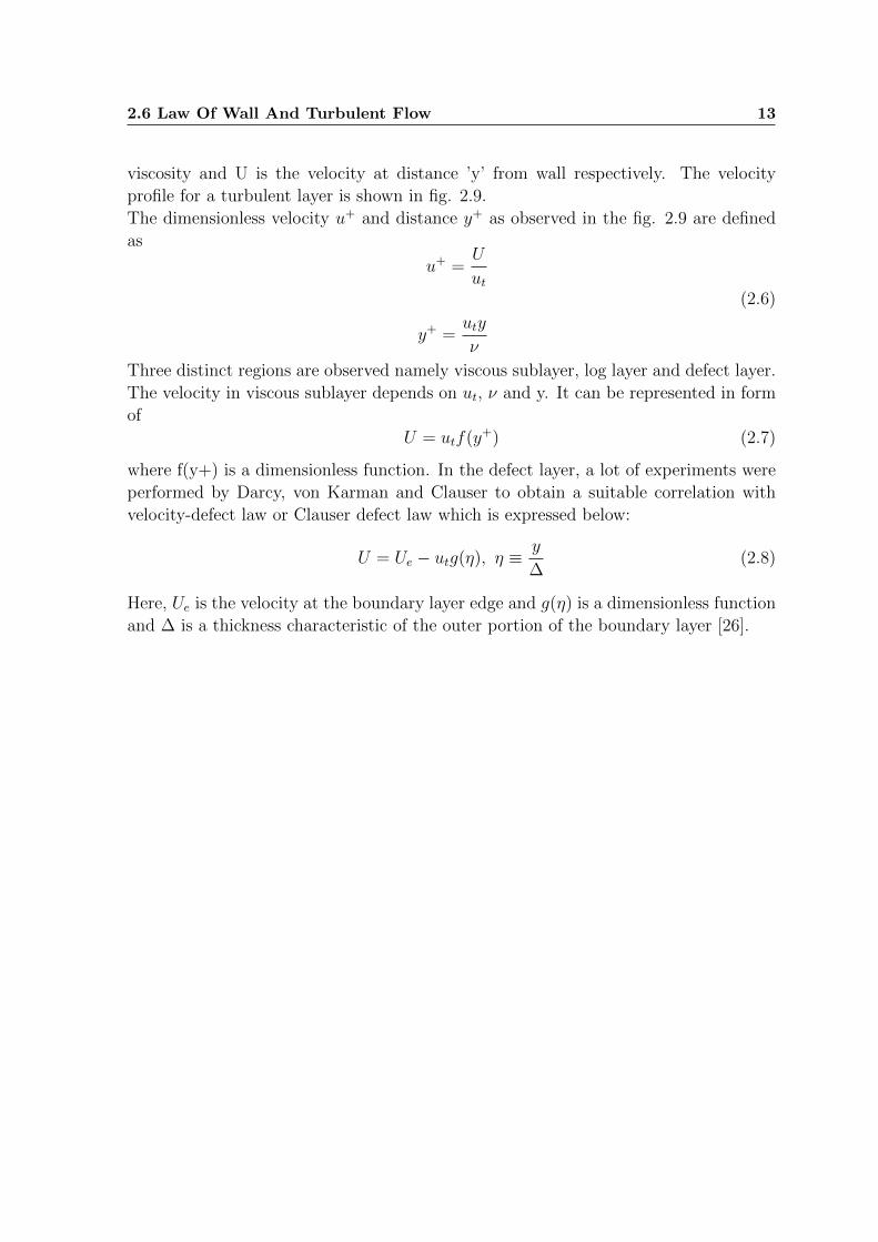
2.6 Law Of Wall And Turbulent Flow 13
viscosity and U is the velocity at distance ’y’ from wall respectively. The velocity
profile for a turbulent layer is shown in fig. 2.9.
The dimensionless velocity u+ and distance y+ as observed in the fig. 2.9 are defined
as
u+ =U
ut
y+ =uty
ν
(2.6)
Three distinct regions are observed namely viscous sublayer, log layer and defect layer.
The velocity in viscous sublayer depends on ut, ν and y. It can be represented in form
of
U = utf(y+) (2.7)
where f(y+) is a dimensionless function. In the defect layer, a lot of experiments were
performed by Darcy, von Karman and Clauser to obtain a suitable correlation with
velocity-defect law or Clauser defect law which is expressed below:
U = Ue − utg(η), η ≡ y
∆(2.8)
Here, Ue is the velocity at the boundary layer edge and g(η) is a dimensionless function
and ∆ is a thickness characteristic of the outer portion of the boundary layer [26].

Chapter 3
Modelling The Turbulence
All models are approximations. Essentially, all models are wrong, but some are useful.
However, the approximate nature of the model must always be borne in mind.
- George Edward Pelham Box -
In this chapter, the theory behind solving the turbulent flows and the relevant physi-
cal equations concerning fluids are discussed. Thereafter, the algebraic zero equation
models for turbulence are described in detail. Furthermore, a brief outline about the
numerical model implementing the staggered grid is discussed. Finally, the concepts
involved in implementation of the models and structure of the program are explained
briefly.
3.1 Equations
The mathematical basis for a comprehensive general purpose model of fluid flow is
formulated from the basic principle of conservation of mass, momentum and energy.
In the conservation laws, the fluid is regarded as a continuum. In the formulation
of equation for mass, momentum and energy, it is assumed that fluid is a continuous
medium contained in a three dimensional space such that every parcel of the fluid, no
matter how small in comparison with the whole body, can be viewed as a continuous
material. For analysis of fluid flows at macroscopic length scales, the molecular struc-
ture of matter and the motions are ignored. The behavior of fluid is described in terms
of macroscopic properties such as velocity, pressure, density and temperature and their
space and time derivatives.
3.1.1 Mass Conservation
The mass conservation equation is derived with an assumption that the rate of increase
of the mass in the fluid element is equal to net rate of flow of mass into fluid element.
In the compact vector notation, it is denoted as

3.2 Approaches 15
∂ρ
∂t=∂(ρui)
∂xi(3.1)
3.1.2 Momentum Conservation
It is derived from the Newton’s second law which states that the rate of change of
momentum of a fluid particles equals the sum of all forces acting on the particle [17].
The equation of momentum conservation is stated as
∂ui∂t
+ uj∂ui∂xj
= fi −1
ρ
∂p
∂xi+ ν
∂2ui∂xj∂xj
(3.2)
where the vector fi represents external forces.
3.2 Approaches
Turbulence simulation, in its purest form can be performed by Direct Numerical Sim-
ulation which is an entirely expensive approach requiring a millions of CPU hours for
relevant Reynolds numbers as described earlier. However, another method known as
Large Eddy simulation can be used. It models the effects of small eddies and resolves
the large, most energetic eddies, the smallest resolved size being of order 102 of the
appropriate dimension of the flow. Another way for resolving the time and space evo-
lution of turbulence within a turbulent flow is achieved by a statistical approach which
is followed in the current study. In this approach, integration of governing equations of
flow in time and derivation of equations for time-averaged flow properties is performed
so as to obtain the Reynolds-Averaged Navier-Stokes equations [9].
3.2.1 Reynolds Averaging
Three types of averaging are most relevant in turbulence modeling namely time average,
spatial average and ensemble average. Time averaging is useful in turbulence which is
stationary in nature i.e. the mean values does not vary with time. Let f(x,t) be an
instantaneous flow variable. Its time average FT (x) is defined as
FT (x) = limT→∞
1
T
∫ t+T
t
f(x, t)dx
Spatial averaging is used in turbulent flow that is uniform in all direction. The spatial
coordinates are averaged. The average is denoted by Fv
FV (t) = limV→∞
1
V
∫V
f(x, t)dV

3.2 Approaches 16
Finally, the ensemble averaging used in turbulent modeling is most general type of
Reynolds averaging suitable for flows that decay in time.
3.2.2 Reynolds -Averaged Navier-Stokes Equations (RANS)
As discussed earlier, the statistical approach is used for solving turbulent flows as
there are often random fluctuations in the flow regime. In order to derive the Reynolds
-Averaged Navier-Stokes Equations from the instantaneous Navier-Stokes equations,
Reynolds decomposition is required. Reynolds decomposition refers to splitting of the
flow variable (like velocity) into a mean component u(x) and fluctuating component
u′.
u(x, t) = u(x) + u′(x, t) (3.3)
Some of the assumptions in derivation of Reynolds -Averaged Navier-Stokes Equations
are as follows:
a) Constant viscosity
b) Density does not depend on pressure
c) The fluid in consideration is Newtonian
d) The fluid is incompressible
e) The mean values of turbulence does not vary with time
Assuming the fluid to be incompressible, the mass conservation equation reduces to
∂ui∂xi
= 0 (3.4)
and the momentum equation is
∂ui∂t
+ uj∂ui∂xj
= fi −1
ρ
∂p
∂xi+ ν
∂2ui∂xj∂xj
(3.5)
Now, each of the instantaneous quantity is split into time-averaged and fluctuating
components. The resulting equations are time-averaged yielding
∂ui∂xi
= 0 (3.6)
∂ui∂t
+ uj∂ui∂xj
+ u′j
∂u′i
∂xj= f i −
1
ρ
∂p
∂xi+ ν
∂2ui∂xj∂xj
(3.7)
The momentum equation can be written as
∂ui∂t
+ uj∂ui∂xj
= f i −1
ρ
∂p
∂xi+ ν
∂2ui∂xj∂xj
−∂u′iu′j
∂xj(3.8)

3.3 The Eddy Viscosity/Diffusivity Concept 17
Upon manipulating further, we obtain
ρ∂ui∂t
+ ρuj∂ui∂xj
= ρf i −∂
∂xj
[−pδij + 2µSij − ρu
′iu′j
](3.9)
Here, µ is viscosity and the mean strain rate tensor sij is given by
sij =1
2
(∂ui∂xj
+∂uj∂xi
)(3.10)
Thus, the above equation represents the Reynolds averaged Navier-Stokes equa-
tion(RANS). The quantity -ρu′ju′i is known as Reynolds stress tensor which is sym-
metric and has six unknown quantities. Thus, we have ten unknown variables in total
i.e. one pressure and three velocity apart from the stress tensor. The total number of
equations are four i.e. one mass conservation and three components of RANS. Hence,
our system is not closed [26].
3.3 The Eddy Viscosity/Diffusivity Concept
The main idea behind Boussinesq’s eddy-viscosity concept, which assumes that, in
analogy to the viscous stresses in laminar flows, the turbulent stresses are proportional
to the mean velocity gradient. So, the Boussinesq’s hypothesis is used to model the
Reynolds stress term. The Reynolds stress tensor is computed as a product of eddy
viscosity and mean strain rate tensor [6].
ρu′ju′i = µt
(∂ui∂xj− ∂uj∂xi
)− 2
3
(K + νt
∂uk∂xk
)δij (3.11)
The above expression can be further written as
ρu′ju′i = 2νtSij −
K
δij(3.12)
where Sij is the mean rate of strain tensor, νt is the turbulence eddy viscosity,
K = 1/2*ρu′ju′i and δij is the Kronecker delta [22].
However, to perform simple computations, the eddy viscosity is often computed in
terms of mixing length which is analogous to the mean free path in a gas. The eddy
viscosity depends on the flow of fluid. Therefore, the eddy viscosity and mixing length
must be specified by an algebraic relation between eddy viscosity and length scales of
the mean flow. The models comprising of algebraic relation are known as zero equation
models i.e. Prandtl mixing length, Baldwin-Lomax and Cebeci-Smith are described in
the corresponding sections [24].

3.4 Zero Equation Models 18
3.4 Zero Equation Models
As mentioned earlier, the zero equation turbulence models implemented in the thesis
work are the models which by definition do not require the solution of any additional
equations and are calculated directly from the flow variables. These models are simple
to use and helpful for simpler geometry. In 1925, Prandtl proposed the mixing length
model for describing the momentum transfer by turbulent Reynolds stresses. There-
after, three modifications of mixing length model was proposed by Van Driest (1956),
Escudier (1966) and Corrsin and Kistler(1954) respectively.
Further, the concept of eddy-viscosity was even more developed by Cebeci and Smith
(1967). Later, Baldwin and Lomax(1978) proposed an alternative algebraic model to
eliminate some of the difficulty in defining a turbulence length scales from the shear
layer thickness apart from incorporating the eddy-viscosity concept of Cebeci-Smith
model. These models are discussed in the following sections.
3.4.1 Prandtl Mixing Length Model
In 1925, Prandtl proposed a mixing length hypothesis. The mixing length conceptually
means that a fluid parcel will conserve its properties for a characteristic length, before
mixing with the surrounding fluid. According to Prandtl, mixing length may be con-
sidered as the diameter of the masses of fluid moving as a whole in each individual case;
or again, as the distance traversed by a mass of this type before it becomes blended
with the neighboring masses [21]. He postulated the shear stress as
τxy = νt
∣∣∣∣∂u∂y∣∣∣∣ (3.13)
where the eddy viscosity, νt is given by
νt = l2mix
∣∣∣∣∂u∂y∣∣∣∣ (3.14)
The mixing length, l = κy with the Karman constant κ=0.40 or 0.41 and the distance
from the wall y. This equation is valid only for wall bounded flows, additionally it
is restricted to smooth surfaces. However, the model fails to provide close agreement
with the measured skin friction for boundary layers. The mixing length relation is not
expected to be constant throughout the boundary layer. Thus, several modifications
to the equation have evolved which are described in the sections below [21].
3.4.2 Van Driest
Van Driest proposed the first modification of the Prandtl mixing length by multiplying
the mixing length with a damping function. The expression for mixing length was an
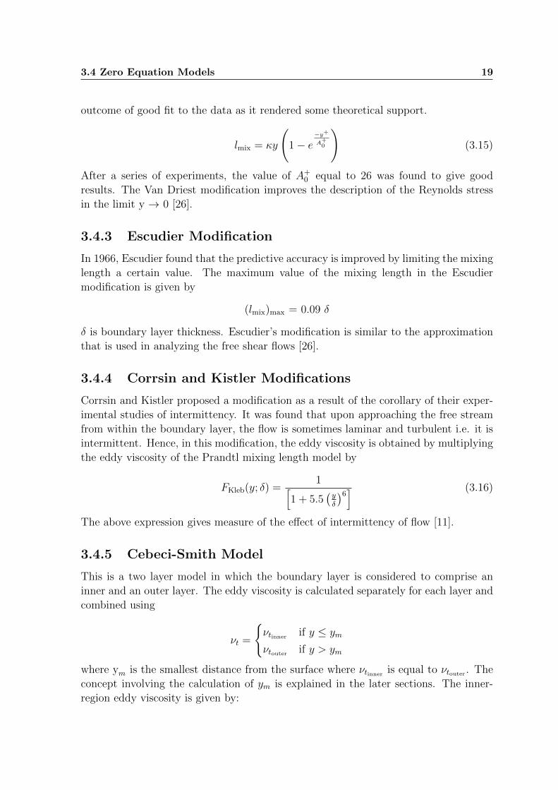
3.4 Zero Equation Models 19
outcome of good fit to the data as it rendered some theoretical support.
lmix = κy
(1− e
−y+
A+0
)(3.15)
After a series of experiments, the value of A+0 equal to 26 was found to give good
results. The Van Driest modification improves the description of the Reynolds stress
in the limit y → 0 [26].
3.4.3 Escudier Modification
In 1966, Escudier found that the predictive accuracy is improved by limiting the mixing
length a certain value. The maximum value of the mixing length in the Escudier
modification is given by
(lmix)max = 0.09 δ
δ is boundary layer thickness. Escudier’s modification is similar to the approximation
that is used in analyzing the free shear flows [26].
3.4.4 Corrsin and Kistler Modifications
Corrsin and Kistler proposed a modification as a result of the corollary of their exper-
imental studies of intermittency. It was found that upon approaching the free stream
from within the boundary layer, the flow is sometimes laminar and turbulent i.e. it is
intermittent. Hence, in this modification, the eddy viscosity is obtained by multiplying
the eddy viscosity of the Prandtl mixing length model by
FKleb(y; δ) =1[
1 + 5.5(yδ
)6] (3.16)
The above expression gives measure of the effect of intermittency of flow [11].
3.4.5 Cebeci-Smith Model
This is a two layer model in which the boundary layer is considered to comprise an
inner and an outer layer. The eddy viscosity is calculated separately for each layer and
combined using
νt =
{νtinner if y ≤ ym
νtouter if y > ym
where ym is the smallest distance from the surface where νtinner is equal to νtouter . The
concept involving the calculation of ym is explained in the later sections. The inner-
region eddy viscosity is given by:

3.4 Zero Equation Models 20
νtinner = ρl2mix
√√√√[(∂U∂y
)2
+
(∂V
∂x
)2]
(3.17)
lmix = κy
(1− e
−y+
A+
)(3.18)
A+ =26√(
1 + ydPdx
ρu2τ
) (3.19)
The coefficient A+ is different than the Van Driest value for an improvement of predic-
tive accuracy in boundary layers with nonzero pressure gradient. The eddy viscosity
in the outer region is given by:
νtouter = αρUeδ∗vFKleb (3.20)
where, α=0.0168, Ue is the boundary layer edge velocity and δ∗v is the velocity thickness
given by
δ∗v =
∫ δ
0
(1− U
Ue
)dy (3.21)
For incompressible flows, it can be noted that velocity thickness is identical to displace-
ment thickness [20]. The FKleb is the Klebanoff intermittency function given by
FKleb(y; δ) =1[
1 + 5.5(yδ
)6] (3.22)
The model is suitable for high-speed flows with thin attached boundary-layers, typically
present in aerospace applications.
3.4.6 Baldwin-Lomax Model
In 1978, Baldwin and Lomax formulated a two layer algebraic equation model. It is
used in applications where the parameters like boundary layer thickness δ, velocity
thickness δ∗v cannot be easily determined. Similar to the Cebeci-Smith, this model
uses inner and outer layer eddy viscosity [6]. The inner and outer viscosity are selected
in a similar criteria like the Cebeci-Smith model.
Here, again ym is defined as the smallest distance from the surface where νtinner is equal
to νtouter . Similar concept is adopted in calculation of the value of ym which is discussed
in the later sections. The inner viscosity is given by
νtinner = (lmix)2|ω|

3.5 Numerical Model 21
where , ω = magnitude of the vorticity vector in three dimensions. The vorticity pa-
rameter is used instead of the velocity gradient for determination of the eddy viscosity.
The mixing length is calculated by Van driest equation
lmix = κy[1− e−y+/A
+0
](3.23)
The outer viscosity is given by
νtouter = ραCcpFWakeFKleb(y; ymax/CKleb) (3.24)
where, Fwake = min (ymaxFmax; CwkymaxU2dif/Fmax)
Fmax = 1κ
(max(lmix|ω|))
where, Fmax is maximum value of lmix|ω| and ymax is the distance at which this
maximum occurs for a given x-position. Here, α=0.0168, Ccp= 1.6, CKleb=0.3, Cwk=1,
κ =0.40 and A+0 =26 respectively.
In this model there is no need to locate the boundary layer edge by calculating the outer
layer length scale in terms of the vorticity instead of the displacement. By replacing
Ueδ∗v in the Cebeci-Smith model by CcpFWake, we have
A) If FWake = ymaxFmax then δ∗v = y2maxωUe
B) If FWake =CwkymaxU2
dif
Fmaxthen δ =
Udif|ω|
An important observation for pipe and channel flow is that subtle difference in a model’s
prediction for Reynolds stress can lead to much larger differences in velocity profile
predictions. This is a common accuracy dilemma with many turbulence models. Both
Cebeci-Smith and Baldwin-Lomax models have been fine-tuned for boundary layer flow
and therefore provide good agreement with experimental data for reasonable pressure
gradients and mild adverse pressure gradients.
3.5 Numerical Model
After the derivation of the relevant mathematical equations mentioned earlier, a nu-
merical model is implemented to solve the developed equations. This is because the
equations are coupled and non-linear partial differential equations. These can be solved
by using the discretization schemes in space and time in a numerical model. Therefore,
a numerical simulator named as DuMux is used in the thesis to solve the equations and
obtain the results [4].

3.5 Numerical Model 22
3.5.1 DuMux
DuMux is a generic framework which is used for simulation of multiphase fluid flow
and transport processes in porous media by the application of continuum mechanical
approaches. DuMux models the concepts, constitutive relations, discretizations and
solvers. Its objective includes delivering top computational performance, high flexibil-
ity, ability to run on single processor systems and highly parallel supercomputers. It
has C++ as its implementation language.
DuMux provides a framework for easy implementation of problems concerning porous
media flow problems with a variety of selection of spatial discretization schemes,
temporal discretization schemes and nonlinear solvers along with the concepts of
model coupling.
DuMux is a module of DUNE (the Distributed and Unified Numerics Environment).
DUNE provides an interface to many existing grid management libraries. It also pro-
vides set of finite element functions and routines for solving partial differential equations
[7].
3.5.2 Box method
In a previous study, the box method of discretization was used to model the turbulent
flows. In this method, the model domain is discretized with a finite element mesh
of nodes and elements. Thereafter, a secondary mesh is created by connecting the
midpoints and barycenteres of the elements surrounding the node to form a box around
it. The finite element mesh divides the box into subcontrol volumes. The finite volume
method is applied to each box so as to obtain the fluxes across the interfaces at the
integration points from the finite element approach.
This method uses the benefit of finite element method which can be used with un-
structured mesh and of finite volume method which is mass conservative. In the later
section of study, the results of box method are compared with the staggered grid to
draw some conclusions.
3.5.3 Discretization In Space Using Staggered Grid
In the current study, a staggered grid discretization method is adopted in the problem
so as to prevent the occurrence of pressure oscillations. In this step, the problem
geometry is split into finite number of volumes. In the cell centered finite volume
method, the pressure and velocities are defined at the nodes of an ordinary control
volume.
∂p
∂x=pe − pwδx
=
(pE+pW
2
)−(pP+pW
2
)δx
=pE − pW
2δx(3.25)

3.5 Numerical Model 23
Figure 3.1: A checker-board pressure field, from [17].
In the fig. 3.1, it is found that the discretized pressure gradients in equation 3.24
have a zero value at all the nodal points in spite of the pressure field exhibiting
spatial oscillations in both directions. This would render zero momentum source in
the discretized equations. This behavior is absolutely unphysical. Moreover, if the
velocities are also represented in grid nodes, the effect of pressure is not evident in
momentum equations. In order to solve the existing problem, a staggered grid is used.
For a staggered grid, the cell centered finite volume method is used for discretization
of the pressure at the center of control volume. The control volume is formed by the
elements of the grid. However, the velocities are defined at the cell faces in between
the nodes i.e. shifted by half the value of a cell and are indicated by arrows.
Figure 3.2: A staggered grid arrangement, from [17].
In the staggered grid arrangement shown in fig. 3.2, the pressure nodes coincide with

3.6 Notes on Implementation 24
the cell faces of u-control volume. The pressure gradient term is given by
∂p
∂x=pP − pWδxu
(3.26)
The checker board field with staggered grid arrangement is considered again and the
appropriate nodal pressure values are subsituted in the (3.25). This yields non-zero
values of pressure in x-direction.
Thus, the staggering of the velocity components prevents an unrealistic behavior of
the discretized momentum equation due to oscillating pressure values. Moreover, the
velocities are obtained at exactly the locations where they are required for the scalar
transport [17].
3.5.4 Discretization in time
In the thesis, an implicit time stepping scheme is used for time discretization. The
equations are solved for primary variables at new time level ti+1. The current time
level is represented as ti [2]. The storage term of each balance equation is given by
∂u
∂t≈ ui+1 − ui
ti+1 − ti= Ai+1ui+1 (3.27)
Here, the vector u contains the unknowns and the A is the coefficient matrix. The
implicit method is adopted as it is unconditionally stable [3].
3.6 Notes on Implementation
In the implementation of some of algebraic models, the knowledge of certain properties
among all the elements in a particular column is required.
3.6.1 General Notes
In the program, at the beginning of a time step, the maximum velocity is evaluated
among all elements of each column. The wall element in the discretized domain is
shown in the fig. 3.3. The value of maximum velocity is stored at the upper or lower
wall element in each column. It depends on the closeness of the element to the wall in
that column. If the element containing maximum velocity is close to the bottom wall
as compared to the upper wall, then the maximum velocity will be stored in bottom
wall and vice-versa. Since, the problem under consideration is symmetric in nature,
the same values of maximum velocities are obtained for the same column.

3.6 Notes on Implementation 25
Figure 3.3: Wall elements in a domain.
The maximum velocity so obtained is essential to calculate the boundary layer thick-
ness and Reynolds number which are required in implementation of the 2nd and 3rd
modification of the Prandtl mixing length models, Cebeci-Smith and Baldwin-Lomax
models.
3.6.2 Concept in Implementation of the Cebeci-Smith and
Baldwin-Lomax Model
In the Cebeci-Smith model, it is required to obtain the values of ym so as to assign
the eddy viscosity a value equal to the inner or outer viscosity as discussed earlier.
ym is defined as the distance from the wall where the inner viscosity is equal to
outer viscosity. So, the value can be determined by equating these viscosities and
solving for ym. However, solving in this manner is not easy due to complex nature
of the expressions for the viscosities. Therefore, another approach is adopted for
computation of ym. In this approach, the difference between both the viscosities are
determined for each element in the column. If the viscosities are equal, their difference
will be zero. Therefore, the aim is to search for elements in the column having lowest
value of this difference. However, it may be difficult to get a zero value. Therefore,
even the lowest absolute value of difference is also considered.
∆ν = min(νtouter − νtinner) (3.28)
In the program, the difference between both viscosities is named as compi. If the

3.6 Notes on Implementation 26
value of compi for the next element in the same column is less than current least
value, then compi is assigned this lesser value. The least value of compi among all
elements in each discretized column is stored in the wall element of the corresponding
column. Finally after evaluating all the elements, the wall distance of the element
having least value of compi in each column is assigned as ym for the corresponding col-
umn of elements. Thereafter, the eddy viscosity is determined for further computations.
Similar approach is adopted in the computation of ym for Baldwin-Lomax Model.
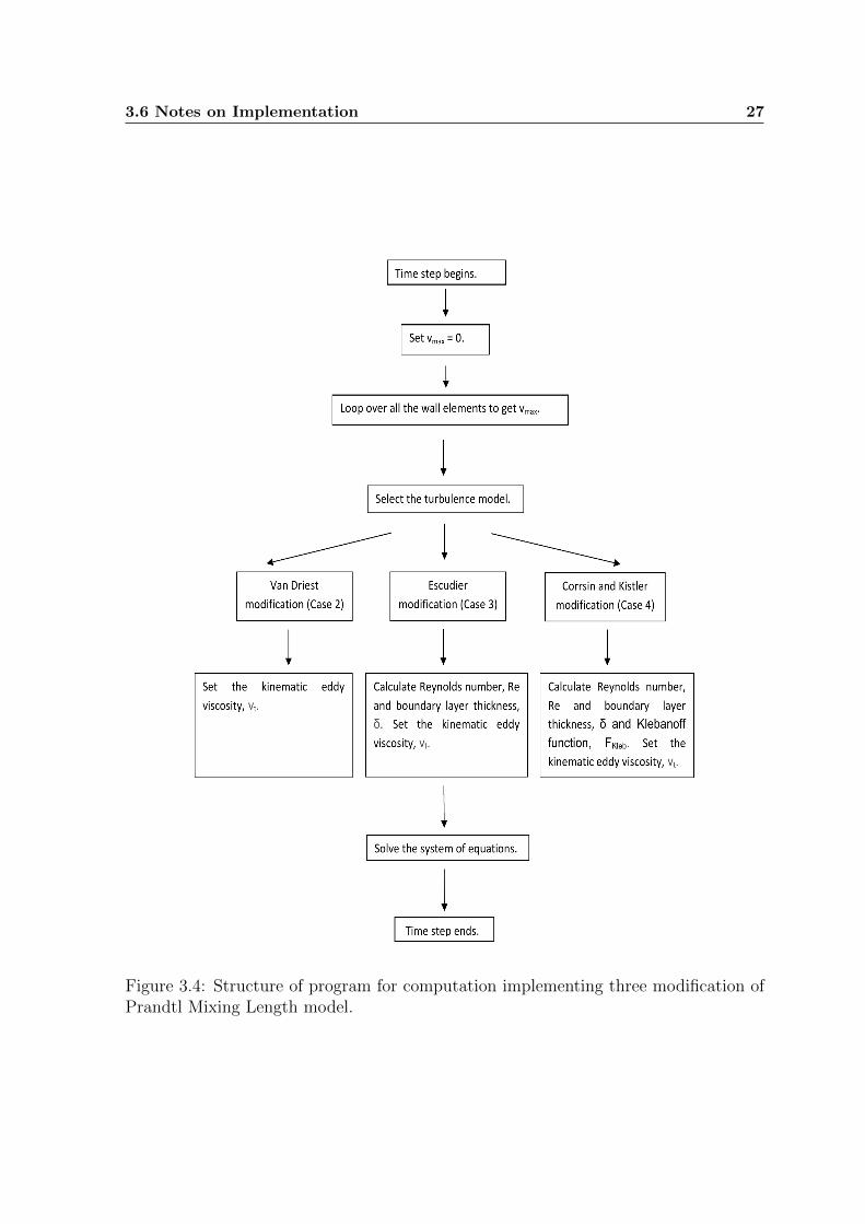
3.6.3 Structure of the Program
The program is created implementing the algorithm for the three modifications of the
Prandtl mixing length model, the Cebeci-Smith and Baldwin-Lomax model. The struc-
ture of the programs are explained in a convenient manner through a schematic rep-
resentation i.e. for the three modifications, Cebeci-Smith Model and Baldwin-Lomax
model.
3.6 Notes on Implementation 27
Figure 3.4: Structure of program for computation implementing three modification ofPrandtl Mixing Length model.

3.6 Notes on Implementation 28
Figure 3.5: Implementation of the Cebeci-Smith Model.

3.6 Notes on Implementation 29
Figure 3.6: Implementation of the Baldwin-Lomax Model.

Chapter 4
Results and Discussion
We must trust to nothing but facts: These are presented to us by Nature, and cannot
deceive. We ought, in every instance, to submit our reasoning to the test of experiment,
and never to search for truth but by the natural road of experiment and observation.
- Antoine Lavoisier, Elements of Chemistry -
In this chapter, the results are computed for a set of input parameters. Thereafter,
the results are obtained and analyzed for different cases. The analysis is performed in
two ways i.e. Analysis of each model Individually and Comparative analysis of all the
models. Finally, conclusions are derived based on the results.
4.1 Model Description
In the current work, the pipe is modeled in a two dimensional domain. The com-
putation of the zero equation models were performed using standard values of the
parameters as depicted below in the table.
Length Thickness Low veloc-
ity
Density Kinematic
viscosity
Time step
10m 0.2469m 2.5m/s 1.21kg/cm3 10−6m2/s 0.1s
End time Pressure Low Re High Re High ve-
locity
7s 105Pa 50 000 500 000 25m/s
The discretized cells that are considered range from values 16 to 64 in each direction
for the problem. The inflow and initial velocity is constant over height, but set to zero
at the upper and lower boundaries, which is called no slip condition. This ensures the
momentum balance. On the right side of pipe, an outflow condition is also chosen for
momentum balance. On the right boundary and outflow of the pipe, the pressure is
set as Dirichlet condition so as to maintain mass balance.

4.2 Individual Analysis 31
4.2 Individual Analysis
In this section, an effort is made to understand the fundamental characteristics of each
model through their outputs. The input values discussed earlier are used in performing
computations for all the models in this section.
4.2.1 Van Driest Modification
The Prandtl mixing length model does not approximate the viscous sub layer properly
especially at the wall. It considers the eddy viscosity in the viscous sublayer uniformly.
The eddy viscosity becomes zero only at the wall where y+ = 0. However, Van Driest
makes the eddy viscosity decrease exponentially as one nears the wall through the
damping function instead of switching it on in the turbulent and sublayer regions
respectively.
Figure 4.1: Velocity profile in the Van Driest modification.
In the fig. 4.1, it can be noticed that the dimensionless velocities attain a higher
value with a coarse discretization of 32 elements compared to a fine discretization of
64 elements for the same value of Reynolds number. The friction velocity which is a
scale representative of velocities close to the solid boundary determines the value of
u+. The friction velocity significantly depends on the discretization of the mesh. This
might be a possible reason for such behavior.

4.2 Individual Analysis 32
The velocity profiles with same discretization and Reynolds number but at different
lengths i.e. 0.3125m and 8.75m are found to be nearly similar.
However, the viscous region in the velocity profile of turbulent layer can not be
noticed. This is because the viscous layer region occurs for y+ less than 10. In the fig.
4.1, we do not obtain values of y+ less than 10 i.e. near the wall. This is because of
the uniform mesh of 32 elements used to discretize the flow in space has less elements
near the wall. In order to obtain less values of dimensionless wall distance, we need to
have more elements near the wall. But an increase in elements will lead to an increase
of computational cost. Therefore, to solve the problem a graded mesh is used.
In the graded mesh, the number of elements is not uniformly distributed along the
vertical direction of discretization in space. A total number of 32 elements in both
directions and a ratio of 1.7 in vertical direction is considered. It has more number
of elements near the wall and the height of each element is 1.7 times the height of
element exactly below it as shown in the fig. 4.2 below.
Figure 4.2: Graded mesh discretization in y axis in pipe.
With a graded mesh, we obtain the curves with less values of dimensionless wall distance
at different lengths of the pipe as shown in fig. 4.3. In this mesh, more number of
elements are located near the wall. Therefore, the wall distance of these elements are
less. The formula of dimensionless wall distance is given by:
y+ =uty
ν(4.1)
Hence, there is a decrease in the value of y+ with lesser values of y and the three
layers in turbulent flow become visible namely viscous sublayer, log layer and defect
layer in fig 4.3.
With higher Reynolds number, the velocities are higher which results in greater values
of dimensionless velocities. Therefore, the curves with higher Reynolds number are

4.2 Individual Analysis 33
Figure 4.3: Plot obtained by Van Driest modification with the graded mesh of 32elements and ratio of 1.7.
placed above the curves with low Reynolds number.
Figure 4.4: Plot of eddy viscosity obtained by Van Driest modification for an uniformmesh of 64 elements.
4.2 Individual Analysis 34
From the fig. 4.4, it is found that the eddy viscosity follows exponential law and
decreases as the wall is approached. However, it increases till a certain point and then
decreases till it reaches the mid thickness of the pipe. This behavior can be attributed to
the fact that eddy viscosity is dependent on the mixing length and velocity gradient.
The velocity gradient initially increases as one moves away from the wall and then
decreases as one approaches the center of pipe. Therefore, the eddy viscosity also
follows a similar pattern.
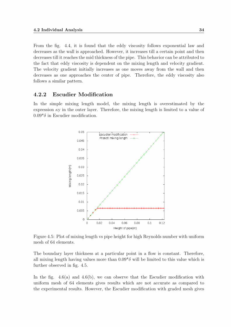
4.2.2 Escudier Modification
In the simple mixing length model, the mixing length is overestimated by the
expression κy in the outer layer. Therefore, the mixing length is limited to a value of
0.09*δ in Escudier modification.
Figure 4.5: Plot of mixing length vs pipe height for high Reynolds number with uniformmesh of 64 elements.
The boundary layer thickness at a particular point in a flow is constant. Therefore,
all mixing length having values more than 0.09*δ will be limited to this value which is
further observed in fig. 4.5.
In the fig. 4.6(a) and 4.6(b), we can observe that the Escudier modification with
uniform mesh of 64 elements gives results which are not accurate as compared to
the experimental results. However, the Escudier modification with graded mesh gives

4.2 Individual Analysis 35
(a) Low Reynolds number (b) High Reynolds number
Figure 4.6: Comparison of velocity profiles by Prandtl simple and Escudier modifica-tion.
more accurate solution as compared to uniform mesh. This is because of more number
of elements in the graded mesh near the wall which improves the results near the
wall region. The same behavior is also observed in the Prandtl mixing length model
with uniform mesh and graded mesh respectively. Also, it can be observed that the
Prandtl mixing length gives better results as compared to Escudier modification for
the experimental setup in consideration.
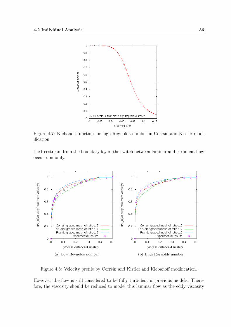
4.2.3 Corrsin and Kistler and Klebanoff Modification
It was observed through experiments by Corrsin and Kistler that the flow approaching
freestream is not fully turbulent in nature. It switches between laminar flow and
turbulent flow at irregular intervals. In order to counter the problem, an intermittency
function was introduced by Klebanoff. This function reduces the eddy viscosity to
model this effect.
From the fig. 4.7, it can observed that Klebanoff function has value of one at the
wall. This implies that the eddy viscosity has the same value and does not decrease in
value. This is justified as the flow is fully laminar near the walls until the freestream is
reached. Therefore, the Klebanoff function does not reduce the eddy viscosity in fully
turbulent flows.
According to Corrsin and Kistler, as the flow moves away from wall and approaches
4.2 Individual Analysis 36
Figure 4.7: Klebanoff function for high Reynolds number in Corrsin and Kistler mod-ification.
the freestream from the boundary layer, the switch between laminar and turbulent flow
occur randomly.
(a) Low Reynolds number (b) High Reynolds number
Figure 4.8: Velocity profile by Corrsin and Kistler and Klebanoff modification.
However, the flow is still considered to be fully turbulent in previous models. There-
fore, the viscosity should be reduced to model this laminar flow as the eddy viscosity
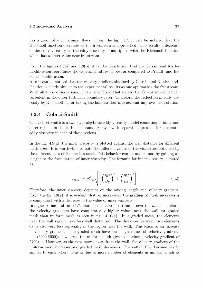
4.2 Individual Analysis 37
has a zero value in laminar flows. From the fig. 4.7, it can be noticed that the
Klebanoff function decreases as the freestream is approached. This results a decrease
of the eddy viscosity as the eddy viscosity is multiplied with the Klebanoff function
which has a lower value near freestream.
From the figures 4.8(a) and 4.8(b), it can be clearly seen that the Corrsin and Kistler
modification reproduces the experimental result best as compared to Prandtl and Es-
cudier modification.
Also it can be noticed that the velocity gradient obtained by Corrsin and Kistler mod-
ification is nearly similar to the experimental results as one approaches the freestream.
With all these observations, it can be inferred that indeed the flow is intermittently
turbulent in the outer turbulent boundary layer. Therefore, the reduction in eddy vis-
cosity by Klebanoff factor taking the laminar flow into account improves the solution.
4.2.4 Cebeci-Smith
The Cebeci-Smith is a two layer algebraic eddy viscosity model consisting of inner and
outer regions in the turbulent boundary layer with separate expression for kinematic
eddy viscosity in each of these regions.
In the fig. 4.9(a), the inner viscosity is plotted against the wall distance for different
mesh sizes. It is worthwhile to note the different values of the viscosities obtained by
the different sizes of the meshes used. This behavior can be understood by gaining an
insight to the formulation of inner viscosity. The formula for inner viscosity is stated
as.
νtinner = ρl2mix
√√√√[(∂U∂y
)2
+
(∂V
∂x
)2]
(4.2)
Therefore, the inner viscosity depends on the mixing length and velocity gradient.
From the fig 4.9(a), it is evident that an increase in the grading of mesh increases is
accompanied with a decrease in the value of inner viscosity.
In a graded mesh of ratio 1.7, more elements are distributed near the wall. Therefore,
the velocity gradients have comparatively higher values near the wall for graded
mesh than uniform mesh as seen in fig. 4.10(a). In a graded mesh, the elements
near the wall region have less wall distances. The distances between two elements
dy is also very less especially in the region near the wall. This leads to an increase
in velocity gradient. The graded mesh have have high values of velocity gradients
i.e. (6000-8000)s−1 whereas the uniform mesh gives a maximum velocity gradient of
2700s−1. However, as the flow moves away from the wall, the velocity gradient of the
uniform mesh increases and graded mesh decreases. Thereafter, they become nearly
similar to each other. This is due to more number of elements in uniform mesh as

4.2 Individual Analysis 38
(a) Inner viscosity plot (b) Outer viscosity plot
.
Figure 4.9: Viscosities for High Reynolds number in Cebeci-Smith model
(a) Wall Distance vs velocity gradient (b) Mixing length vs inner viscosity
Figure 4.10: Plot for High Reynolds number in Cebeci-Smith model.
compared to graded mesh in the region considerably away from wall. These reasons
may form the basis for decrease of inner viscosity with an increase in grading of mesh
in Cebeci-Smith model.

4.2 Individual Analysis 39
Also, from the fig. 4.10(b), it is interesting to note the resemblance in behavior of
the inner viscosity with wall distance and inner viscosity with mixing length for the
different mesh considered. This can be explained on the fact that the mixing length
is predominantly a function of the velocity gradient and the velocity gradient further
determines the behavior of the inner viscosity. So, this might be a possible explanation
for obtaining similar curves are obtained in these cases.
In the fig. 4.9(b), the outer viscosity is plotted against the wall distance for different
size of meshes at 38.125m. The formula of outer viscosity is stated below.
νtouter = αρUeδ∗vFKleb
It is observed that the outer viscosity decreases with an increase in the wall distance.
This behavior can be attributed to the fact that the outer viscosity depends on the
Klebanoff function. In the fig. 4.11(a), it can be clearly seen that the Klebanoff function
follows a pattern similar to the outer viscosity when plotted against wall distance.
Also, it is observed that the values of outer viscosity increases with an increase in
the grading of the mesh. The results obtained with graded mesh differ a lot from the
results obtained with uniform mesh until the free stream is approached. This can
be explained on the fact that outer viscosity is directly proportional to the velocity
thickness and other parameters. In the fig. 4.11(b), it can be observed that velocity
thickness increases with an increase in grading of the mesh. Therefore, the outer
viscosity with a uniform mesh has a lower value due to lower value of the velocity
thickness. Therefore, these reasons might form the basis for such behavior of the outer
viscosity.
In the fig. 4.12, the eddy viscosity is plotted against the wall distance. Initially, the
eddy viscosity adopts the values of inner viscosity. The point at which the inner
viscosity becomes equal to the outer viscosity, the eddy viscosity switches to outer
viscosity. Upon comparison of the curves for inner viscosity and outer viscosity, it can
be found that the eddy viscosity takes the value of outer viscosity as compared to
inner viscosity after a certain wall distance.
In the fig. 4.13(a) and 4.13(b), the dimensionless wall distance is plotted against the
dimensionless velocity. There occurs a deviation near the end of the boundary layer as
can be seen from the plot. This is because, such a defect from the log-law in the outer
region of the boundary layer is also observed in various experimental results. Thus,
this region is named as ’defect layer’. As its name implies, the logarithmic profile, so
that there is a defect.
Also, as mentioned earlier, with an increase in grading of the mesh, the region of curve
near the wall is obtained. Furthermore, it is noticed that the curves of higher Reynolds
number are placed above the curves with lower Reynolds number.

4.2 Individual Analysis 40
(a) Klebanoff funciton (b) Velocity thickness at 38.125m length of pipe
Figure 4.11: Plot for High Reynolds number in Cebeci-Smith model
Figure 4.12: Kinematic eddy viscosity plot with high Reynolds number in Cebeci-Smithmodel.

4.2 Individual Analysis 41
(a) Low Reynolds number (b) High Reynolds number
Figure 4.13: Logarthmic law for velocity at 19m.
Figure 4.14: Velocity profile for high Reynolds number.
This can be attributed to the higher values of dimensionless velocity with higher
Reynolds number as compared to lower Reynolds number at the same wall distances.
In the fig. 4.14, it can be observed that the Cebeci-Smith model produces more accurate

4.2 Individual Analysis 42
results as compared to the simple Prandtl mixing length model. This is because it uses
inner viscosity and outer viscosity which causes better reproduction of velocities with
the exact solution. However, the results obtained by Cebeci-Smith model assume more
similarity with the experimental results after grading the mesh by a factor of 1.2.
4.2.5 Baldwin-Lomax
In this section, some of the properties of the model are highlighted to explain certain
behavior of the outputs. The input values as discussed earlier are considered for
producing outputs by the Baldwin-Lomax model.
In the fig. 4.15(a), it can be observed that the inner viscosity follows a pattern similar
to the Cebeci-Smith model i.e. it decreases upon increasing the grading of mesh.
(a) Inner viscosity plot (b) Outer viscosity plot
Figure 4.15: Viscosities for High Reynolds number in Baldwin-Lomax model
This can explained on the basis that inner viscosity in both the models have same
formulation. The reason for the similar behavior of the inner viscosity explained in
the Cebeci-Smith also holds true in this case too.
In the fig. 4.15(b), it is noticed that the outer viscosity decreases upon increasing
the grading in mesh. In other words, an increase in number of elements near the
wall produces relatively low values of outer viscosity. This can be better understood
better by following the process of computation in the Baldwin-Lomax model. With
higher grading, the elements and the corresponding wall distances are of small size in

4.2 Individual Analysis 43
the region near the wall. Therefore, the product of mixing length and vorticity which
determines the value of Fmax attains lesser values.
Fmax = 1κ
(max(lmix|ω|))
This might be a possible explanation for the decrease in value of lmix|ω| with an increase
in grading of the mesh as noticed in fig. 4.16(a). But, the ymax being the wall distance
at which the Fmax attains maximum value remains constant in all the cases.
(a) lmix|ω| plot (b) Fwake plot
Figure 4.16: Plots for High Reynolds number in Baldwin-Lomax model
Fwake = min (ymaxFmax; CwkymaxU2dif/Fmax)
νtouter = ραCcpFWakeFKleb(y; ymax/CKleb)
Now, the Fwake further depends on the value of Fmax.
So, it is again noticed that the value of the Fwake decreases as the grading of the mesh
increases in the fig. 4.14(b). Finally, the outer viscosity being proportional to Fwake
also follows the similar pattern.
In the fig. 4.17(a), the eddy viscosities are plotted against the wall distances. The
eddy viscosity changes adopting values from inner viscosity to outer viscosity at the
distance ym where both the viscosities attain similar values as mentioned earlier.
The ym can be determined graphically by superimposition of the outer viscosity curve
on the inner viscosity curve as shown in fig. 4.17(b). Thereafter, ym can be computed
as the distance of point where the curve changes its shape significantly from the wall.

4.2 Individual Analysis 44
(a) Plot of Kinematic eddy viscosity (b) Superimposed plot of inner and outer viscos-ity
Figure 4.17: Viscosities for High Reynolds number in Baldwin-Lomax model
(a) Low Reynolds number (b) High Reynolds number
Figure 4.18: Velocity profiles in Baldwin-Lomax model
Moreover, the curve of eddy viscosity obtained in current case is in total agreement
with the curve of Baldwin-Lomax model.

4.3 Comparative Analysis 45
In the fig. 4.18(a) and fig. 4.18(b), it can be seen that the velocity profile improves
more towards the experimental results as the grading of mesh is increased.
With a high grading, more elements are located near the wall. Therefore, the velocity
profile with graded mesh near the wall are more accurate as compared to the uni-
form mesh. Also, the overall velocity profile tends to have more similarity with the
experimental results.
Also, it is necessary to note that the Cebeci-Smith model as discussed earlier renders
accurate velocity profiles with a grading of 1.2 as compared to Baldwin-Lomax with a
grading of 1.7.
4.3 Comparative Analysis
The objective of this section is to draw conclusions by making a comparison of the
results obtained by all the models.
4.3.1 All Models
The velocity profile of all the five models considered in the current study are analyzed.
The details of the input considered are similar to that discussed earlier.
(a) Uniform mesh of 64 elements (b) Graded mesh of ratio 1.7
Figure 4.19: Velocity profiles for high Reynolds number
In the plot 4.19(a),the velocity profiles obtained by all the method are compared for
high Reynolds number using an uniform mesh of elements. It is observed that the Van
Driest and Cebeci-Smith render results that are close to the experimental solution as

4.3 Comparative Analysis 46
compared to other methods. As discussed earlier, the results obtained by Escudier
and Baldwin Lomax differ a lot from experimental solution for the uniform mesh.
However, the Corrsin and Kistler modification gives better result as compared to the
Escudier and Baldwin-Lomax. This is due to the inclusion of intermittency factor in
the model which improves the result.
On a broader scale, the results obtained with uniform mesh by all the methods do
not produce accurate solution. The deviation from the experimental solution begins
as the flow begins to move away from the wall. This is because of less concentration
of elements near the wall. With high Reynolds number, there is development of the
turbulent boundary layer in addition to laminar boundary layer near the wall.
The turbulent boundary layer consists of regions marked with irrotational flows and
vortices. These vortices pump the low momentum fluid near the wall in upward
direction. This upwelling generates Reynolds shear stresses. Moreover, there is
occurrence of intermittent characteristics in the upper portion of the turbulent
boundary layer. Therefore, more number of elements are required near the wall to
simulate these behaviors and obtain relatively better results.
(a) Uniform mesh of 64 elements (b) Graded mesh of ratio 1.7
Figure 4.20: Velocity profiles for low Reynolds number
In the fig. 4.19(b), a graded mesh with ratio of 1.7 is used for comparison of the
velocity profiles for all the models under consideration with high Reynolds number.
This mesh has more number of elements distributed near the wall. From the fig.
4.19(b), it can observed that the results obtained by the graded mesh for all the models

4.3 Comparative Analysis 47
are comparatively better than the previous case. Baldwin-Lomax and Corrsin-Kistler
render the best results among all the models for graded mesh.
In the fig. 4.20(a), an uniform mesh is used to plot the velocity profiles for the
models with low Reynolds number. The results obtained by Cebeci-Smith and Van
Driest modification are more close to the experimental solution as compared to other
methods. The velocity profile of Escudier modification has a lot of deviation from
the experimental solution. This might be attributed to the fact that it is the simple
mixing length model with the mixing length limited to a value of 0.09δ. It does not
include the intermittency property of flow as it approaches the free stream, inner and
outer viscosities for turbulent behavior. The results produced by Baldwin-Lomax are
more accurate in the region near the wall and freestream. However, the solution by
Corrsin and Kistler modification are more close to the experimental solution near the
freestream.
In the fig. 4.20(b), a graded mesh with a ratio of 1.7 is used for the same low Reynolds
number. With a higher concentration of elements near the wall in the mesh, the velocity
profile is nearly similar to the experimental values near the wall for all the models
except the Van Driest and Cebeci-Smith model. Therefore, the results obtained by
graded mesh are comparatively better than the uniform mesh. Again, the Baldwin-
Lomax and Corrsin-Kistler render the best results among all the models.
4.3.2 Logarithmic Velocity profile
In this section, the logarithmic law of wall is obtained and analyzed for all the models
under consideration. In the fig. 4.21(a) and 4.21(b), the logarithmic velocity profile
of all the models in current study are plotted. It can be observed that the curves of
Baldwin-Lomax, Van Driest and Cebeci-Smith are nearly identical till the outer layer
of the log layer. Similar behavior is also observed for the Escudier modification and
Corrsin and Kistler modification.
Also, it is worthwhile to note that dimensionless velocities obtained by the Cebeci-
Smith, Van Driest and Baldwin-Lomax model are more than Escudier modification
and Corrsin and Kistler modifications.
4.3.3 Staggered and Regular Grid
In this section, comparison are made between staggered grid and Box method for the
Van Driest modification and the Baldwin-Lomax model.
In the fig 4.22(a) and 4.22(b), the velocity profiles are compared between box method
and staggered grid for the Van Driest modification. In an uniform mesh, with a low
Reynolds number, it can be observed that the velocity profile with a staggered grid is
more accurate than the box method upon comparison with the experimental results.

4.3 Comparative Analysis 48
(a) Low Reynolds number (b) High Reynolds number
Figure 4.21: Logarithmic velocity profiles.
(a) Low Reynolds number (b) High Reynolds number
Figure 4.22: Velocity profiles comparison between staggered Grid and Box method forVan Driest modification.

4.3 Comparative Analysis 49
(a) Low Reynolds number (b) High Reynolds number
Figure 4.23: Velocity profiles comparison between staggered Grid and Box method forBaldwin-Lomax model.
Even, with a uniform mesh and high Reynolds number, the velocity profile obtained by
staggered grid is better than box method especially near the wall. However, the veloc-
ity profile obtained with graded mesh are similar for the staggered grid and box method.
In the fig. 4.23(a) and 4.23(b), the velocity profiles are analyzed between box method
and staggered grid for the Baldwin-Lomax model. In an uniform mesh, with low and
high Reynolds number, the velocity profile with staggered grid renders result that is
more close to the experimental results as compared to box method. But again, with
a graded mesh, the results obtained for staggered grid and box method are nearly
identical.
The advantage of staggered grids are more accurate pressure gradient and prevention
of the pressure oscillations. In the regular grid of box method, the pressure gradient is
approximated with two alternate grid points when a central difference scheme is used.
Therefore, a wavy pressure field is felt like a uniform pressure field by the momentum
equation. However, in a staggered grid, the pressure gradient is approximated by
the difference of pressures between two adjacent grid points. So, the pressure having
oscillatory behavior does not become an uniform pressure field and could not become
a possible solution. The discretized continuity equation given by:
un+1i+1/2,j − u
n+1i−1/2,j
∆x+vn+1i,j+1/2 − v
n+1i,j−1/2
∆y= 0; (4.3)

4.3 Comparative Analysis 50
(a) Low Reynolds number (b) High Reynolds number
Figure 4.24: Plot of Pressure with Pipe length for box method.
(a) Low Reynolds number (b) High Reynolds number
Figure 4.25: Plot of Pressure with Pipe length for Staggered grid.
contains differences of the adjacent velocity components which prevents a wavy velocity
field from the satisfying the continuity equation. Therefore, the accuracy of the solution
increases with the use of a staggered grid.
In the fig. 4.24(a) and 4.24(b), it can be seen that the pressure oscillations occur in
the box method for both Van driest and Baldwin-Lomax model respectively. However,
in fig. 4.25(a) and 4.25(b), it is observed that there is no pressure oscillations with

4.3 Comparative Analysis 51
the staggered grid.
The staggered grid is known to prevent any occurrence of pressure oscillations. Stag-
gered grid automatically couples the grid scale to pressure to the remainder of the
solution. Therefore, it does not suffer from the problem of pressure oscillation. The
truncation error for (4.3) is O (∆x2, ∆y2). So, the pressure gradient evaluated at the
cell faces is second order accurate. The pressure gradient evaluated at the cell faces
are second order accurate. So, the staggered grid is more accurate.

Chapter 5
Summary And Outlook
The trouble with research is that it tells you what people were thinking about yesterday,
not tomorrow. It’s like driving a car using a rear view mirror.
- Bernard Loomis -
The prime objective of the current study is related to the modeling of turbulence
in free flowing gas phase. In this regard, five different models of turbulence were
implemented through the framework of DuMux and using a staggered grid.
Initially, the analysis was performed for each of the models individually. The
characteristic features of the models were highlighted in the analysis. It included
behavior of the parameters like mixing length, inner viscosity, outer viscosity and
Klebanoff function. Also, there was an improvement in the accuracy of the results
was noticed upon progressing from Van Driest modification to Baldwin-Lomax model.
Firstly, in the Van Driest model, the exponential law of eddy viscosity was put into
practice. Secondly, in the Escudier modification, the restriction on the mixing length
was employed. This lead to an enhancement in the result as compared to simple
mixing length model. Thirdly, in the Corrsin and Kistler and Klebanoff modification,
the intermittency of turbulent flow as it approaches free stream was applied through
the Klebanoff function. This also resulted in more accurate results upon comparing
with the experimental values. Fourthly, the Cebeci-Smith model was also executed
with the inner and outer viscosities. Finally, the Baldwin-Lomax model consisting of
additional parameters was also realized.
Furthermore, all the models were analyzed in a combined manner. The models like
Baldwin-Lomax and Corrsin and Kistler modification performed the best among all
the models under consideration. Moreover, the logarithmic velocity profile of all the
models were analyzed too. Finally, a comparison was made between staggered grid
and the box method especially for the Van Driest modification and Baldwin-Lomax
models. As expected, the accuracy achieved by the staggered grid was better than the
box method. Also, it was found that the pressure oscillations observed in box method

53
were absent in the staggered grid. Additionally, it was found that the results obtained
by all the models for low Reynolds number were relatively more accurate than the
ones obtained with high Reynolds number. More importantly, all the analysis were
carried out with different grading of the mesh and an attempt was made to understand
the observed behaviors.
On a general note, it can be inferred that the algebraic models give good results for
simple flows. The algebraic models are fast and robust in computation. They require
information pertaining to the boundary layer properties.
A possible field of research will be devising and implementing a method to model
separated flows by Cebeci-Smith and Baldwin-Lomax models. As the boundary layer
separates, it is necessary to solve the full Reynolds-averaged Navier-Stokes equation.
Several schemes like MacCormack schemes which are second order accurate in space
and time can be used for this purpose. This scheme involves a predictor step and
a corrector step. Other schemes like Jameson and Mavriplis can be used. It is a
symmetrical scheme in which discretization is performed by a Runge-Kutta method
having five stages. Therefore, the implemented method should be able to model all the
separated regions successfully.
Another approach that can be used to calculate flows with separation region is by a
combination of the Baldwin-Lomax and Smagorinsky turbulence models. The Baldwin-
Lomax model can be used near the wall as it gives good result near the walls. Then,
from the end of inner layer to the core flow region, a mix of Baldwin-Lomax and
Smagorinsky model can be used for modeling of the flow.
With these implementations, it would be important to study different fields like
modeling the water hammer and flow over airfoil.
Lastly, all the findings were only for the particular experimental setup as mentioned
earlier. Another possibility of future work can be computations of results for different
experimental setup i.e. varying the pipe height, length, inlet velocity, pressure and
boundary conditions. The results so obtained can be compared with the experimental
results for similar experimental setup.

Bibliography
[1] http://www.brookfieldengineering.com/education/what-is-viscosity.asp.
[2] http://www.cfm.brown.edu/people/gk/chap6/node15.html.
[3] http://www.mathematik.uni-dortmund.de/ kuzmin/cfdintro/lecture8.pdf.
[4] Dumux homepage. http://www.dumux.org/.
[5] Aerospace Mechanical and Mechatronic Engineering. Aerodynamics for students.
University of Sydney, 2005.
[6] Celik, I. B. Introductory turbulence modeling. West Virginia university , Me-
chanical & Aerospace Engineering Department, P.O. Box 6106, Morgantown, WV
26506-6106, December 1999.
[7] Department of hydromechanics and hydrosystems modelling, Stuttgart. Dumux
handbook. http://dumux.org.
[8] Glenn research center, National Aeronautics and Space Adminstration, USA.
Boundary layer.
[9] Imperial College London. Research: Turbulent flow modelling and simulation.
http://www3.imperial.ac.uk/tfms/turbulentflowmodelling.
[10] Kenryk Kudela. Viscous flow in pipe.
[11] Knopp, T. Boundary layer flows, the logarithmic law of the wall ,mixing length
model for turbulent viscosity. DLR Gottingen, November 2008.
[12] McDonough, J. Lectures in elementary fluid dynamics: Physics, mathematics and
application. Deaprtment of Mechanical Engineering and Mathematics, University
of kentucky, Lexington, KY 40506-0503, S. 163, 2009.
[13] National Programme on Technology Enhanced Learning. Fluid mechanics tutorial
no. 3. Ministry of HRD, Government of India.
[14] National Programme on Technology Enhanced learning, Ministry of HRD, Gov-
ernment of India. Lecture -1: Fundamental aspects, viscous incompressible flow.
54

BIBLIOGRAPHY 55
[15] Tu, Jiyuan, and Inthavong, Kiao, and Ahmadi, Goodarz. Computational fluid and
particle dynamics in the human respiratory system. Springer Dordrecht, 2013.
[16] Veldman, A. Boundary layers in fluid Dynamics. Faculty of mathematics and
natural sciences, 2011-2012.
[17] Versteeg, H. and Malalasekera, W. An Introduction to Computational Fluid Dy-
namics: The Finite Volume Method. Pearson Education Limited, 2007.
[18] Wagner, H. and Sagaut. Large-Eddy Simulation for Acoustics. Cambridge Uni-
versity Press.
[19] Widera, P. Study of sediment transport processess using reynolds avergaed navier-
stokes and large eddy simulation. PhD Thesis, Faculty of Engineering, Vrije
Universiteit Brussel, S. 205, 2011.
[20] Wikipedia. Cebecismith model, December 2013.
[21] Wikipedia. Mixing length model. Wikipedia, November 2013.
[22] Wikipedia. Turbulence modeling. 2013.
[23] Wikipedia. Boundary layer. February 2014.
[24] Wikipedia. Reynolds-averaged navierstokes equations, March 2014.
[25] Wikipedia. Turbulence, May 2014.
[26] Wilcox, D. Turbulence Modeling for CFD: Text. Turbulence Modeling for CFD.
DCW Industries, Incorporated, 2006.


