
MBELLA, KINGE KEKA, Ph.D. Data Collection Design for Equivalent Groups Equating: Using a Matrix Stratification Framework for Mixed-Format Assessment. (2012) Directed by Drs. Richard M. Luecht and Micheline Chalhoub-Deville. 177 pp.
Mixed-format assessments are increasingly being used in large scale standardized
assessments to measure a continuum of skills ranging from basic recall to higher order
thinking skills. These assessments are usually comprised of a combination of (a)
multiple-choice items which can be efficiently scored, have stable psychometric
properties, and measure a broader range of concepts; and (b) constructed-response items
that measure higher order thinking skills, but are associated with lower psychometric
qualities and higher cost of test administration and scoring. The combination of such
item types in a single test form complicates the use of psychometric procedures,
particularly test equating which is a vital component in standardized assessment.
Currently there is very little research that examines the robustness of current
equating methodologies for tests that employ a mixed format. The purpose of this
dissertation was twofold. The first goal of this research was to present evidence on the
use of a predictive stratification framework based on an already available covariate to
create equivalent groups. The second goal was to present supporting evidence on an
appropriate data collection designs for mixed-format test equating.
AP data from an AP Chemistry test and an AP Spanish Language test were
obtained, covering a three year period. Two categorical covariates were created based on
average AP score and school size from previous years. A 5 X 5 crosstab stratified cluster
sampling matrix was created from the two new categorical variables and used to evaluate

the accuracy and precision of mixed-format observed-score equipercentile equating. Six
research conditions were investigated using a re-sampling framework as follows: (a) two
random stratified cluster groups equating designs, (b) two test form conditions, (c) four
sampling rates, (d) two AP test subjects, (e) two sampling frame conditions, and (f) three
equating designs.
There were two major findings summarized from the 500 bootstrap replications in
each design condition. Firsts, the random stratified cluster group equating design had the
most conditions with total equating error less than .1 standard deviation unit of the raw
score scale. Second, Model 1, in which the equating function was estimated using a
smaller sample and the larger sampling frame, was more accurate than Model 2 where the
equating function was based on two equivalent samples from the stratified matrix.
An unanticipated but interesting finding was that equating estimates from AP
Spanish was more accurate compared to those from AP Chemistry despite the fact that
the dis-attenuated correlation coefficient between the multiple-choice and constructed-
response section was higher (unity) in AP Chemistry than in AP Spanish.

DATA COLLECTION DESIGN FOR EQUIVALENT GROUPS EQUATING:
USING A MATRIX STRATIFICATION FRAMEWORK
FOR MIXED-FORMAT ASSESSMENT
by
Kinge Keka Mbella
A Dissertation Submitted to the Faculty of The Graduate School at
The University of North Carolina at Greensboro in Partial Fulfillment
of the Requirements for the Degree Doctor of Philosophy
Greensboro 2012
Approved by Committee Co-Chair Committee Co-Chair

ii
APPROVAL PAGE
This dissertation has been approved by the following committee of the Faculty of
The Graduate School at The University of North Carolina at Greensboro.
Committee Co-Chair Committee Co-Chair Committee Members ____________________________ Date of Acceptance by Committee ____________________________ Date of Final Oral Examination

iii
ACKNOWLEDGMENTS
The successful completion of this personal and professional achievement was
only possible with the support and encouragements I received from my entire family,
friends, professors in graduate school and professional colleagues during this six year
journey.
I would like to specially acknowledge the support and contributions I received
from the following individuals: The members of my dissertation committee, Co-chairs,
Dr. Richard Luecht (for keeping me focused) and Dr. Micheline Chalhoub-Deville (for
being a great advocate and advisor during my tenure at UNCG). Committee members,
Dr. Rick Morgan (who always made time to meet and redirect me), Dr. Terry Ackerman
(for all the encouragements), and Dr. Ourania Rotou (for giving me the inspiration and
support in designing this dissertation).
Also, I want to thank Dr. Wayne Camara and all his staff at College Board for
allowing me to use and preparing the AP datasets used in this dissertation.
Finally none of this would have been possible without the full support of my
beloved wife, Valerie Mbella, and my patient boys, Keka Mbella and Luby Mbella.
iv
TABLE OF CONTENTS
Page LIST OF TABLES ............................................................................................................. vi LIST OF FIGURES ........................................................................................................... ix LIST OF ACRONYMS AND ABBREVIATIONS .......................................................... xi CHAPTER I. INTRODUCTION ................................................................................................1
1.1. Background ...........................................................................................1 1.2. Rationale for Research ..........................................................................3 1.3. Purpose and Research Questions ..........................................................8 1.4. Overview of Dissertation ....................................................................11
II. LITERATURE REVIEW ...................................................................................14
2.1. Overview of Equating .........................................................................15 2.2. Review of Data Collection Designs ....................................................18 2.3. Equivalence of MC and CR Formats ..................................................22 2.4. Research on Mixed-Format Equating .................................................36 2.5. Sampling Designs and Variance Estimation .......................................48
III. METHODOLOGY .............................................................................................63
3.1. Study Methodology .............................................................................65 3.2. Operational Dataset Transformation ...................................................67 3.3. Experimental Test Forms ....................................................................73 3.4. Equating Procedures ...........................................................................82 3.5. Evaluation Criteria and Data Analyses ...............................................88 3.6. Re-sampling Study ..............................................................................98
IV. RESULTS .........................................................................................................105
4.1. Criterion Equating Analysis ..............................................................105 4.2. Results—Research Question 1 ..........................................................115 4.3. Results—Research Question 2 ..........................................................132 4.4. Results—Research Question 3 ..........................................................145

v
V. DISCUSSION ...................................................................................................148
5.1. Overview of Methodology ................................................................148 5.2. Summary of Major Findings .............................................................150 5.3. Practical Implications of Results ......................................................156 5.4. Limitations of Research and Future Direction ..................................158
REFERENCES ................................................................................................................164 APPENDIX A. OPERATIONAL TEST FORM ..........................................................170 APPENDIX B. CLASSIFICATION CONSISTENCY ................................................172

vi
LIST OF TABLES
Page
Table 2.1. Summary of Traub’s Meta-analysis on Construct Equivalence ...................32 Table 3.1. Population and Sampling Frame for AP Chemistry .....................................72 Table 3.2. Population and Sampling Frame for AP Spanish Language .........................73 Table 3.3. Standardized Effect Size for Alternate Experimental Mixed- Format Pairs ..............................................................................................77 Table 3.4. AP Chemistry 2009 Operational and Experimental Test Forms Statistics ...................................................................................................78 Table 3.5. AP Spanish 2009 Operational and Experimental Test Forms Statistics ...................................................................................................79 Table 3.6. AP Spanish 2010 Operational and Experimental Test Forms Statistics ...................................................................................................80 Table 3.7. AP Chemistry 2010 Operational and Experimental Test Forms Statistics ........................................................................................81 Table 3.8. Operational and Experimental Cutoff Scores for Mixed- Format AP Grades....................................................................................90 Table 3.9. Equating Design Conditions .........................................................................92 Table 3.10. Summary of Effective Sample Sizes for Chemistry .....................................93 Table 3.11. Summary of Effective Sample Sizes for Spanish .........................................94 Table 3.12. Summary for NEAT Design Experimental Populations Chemistry ................................................................................................102 Table 3.13. Summary for NEAT Design Experimental Populations Spanish ...................................................................................................103 Table 4.1. Equipercentile SG Equated Moments Chemistry EE_HH 2009.................106 Table 4.2. Equipercentile SG Equated Moments Chemistry EH_HE 2009.................106

vii
Table 4.3. Equipercentile SG Equated Moments Chemistry EE_HH 2010.................106 Table 4.4. Equipercentile SG Equated Moments Chemistry EH_HE 2010.................107 Table 4.5. Equipercentile SG Equated Moments Spanish EE_HH 2009 .....................107 Table 4.6. Equipercentile SG Equated Moments Spanish EH_HE 2009 .....................107 Table 4.7. Equipercentile SG Equated Moments Spanish EE_HH 2010 .....................108 Table 4.8. Equipercentile SG Equated Moments Spanish EH_HE 2010 .....................108 Table 4.9. Weighted Averages by Sampling Condition and Design for Chemistry EE_HH (ES = 0.15) .............................................................126 Table 4.10. Weighted Averages by Sampling Condition and Design for Chemistry 2009 EH_HE (ES = 0.03) ....................................................127 Table 4.11. Weighted Averages by Sampling Condition and Design for Spanish 2009 EE_HH (ES = 0.24) ........................................................128 Table 4.12. Weighted Averages by Sampling Condition and Design for Spanish 2009 EH_HE (ES = 0.15) ........................................................129 Table 4.13. Weighted Averages by Sampling Condition and Design— Chemistry 2010 .....................................................................................146 Table 4.14. Weighted Averages by Sampling Condition and Design— Spanish 2010 .........................................................................................146 Table A.1. Descriptive Statistics for AP Operational Test Form: Spanish Language ................................................................................................170 Table A.2. Descriptive Statistics for AP Operational Test Form: Chemistry ...............................................................................................171 Table B.1. AP Grade Classification Consistency 2009 for Chemistry EE_HH ...................................................................................................172 Table B.2. AP Grade Classification Consistency 2009 for Chemistry EH_HE ...................................................................................................173

viii
Table B.3. AP Grade Classification Consistency 2009 for Spanish EE_HH ...................................................................................................174 Table B.4. AP Grade Classification Consistency 2009 for Spanish EH_HE ...................................................................................................175 Table B.5. AP Grade Classification Consistency Chemistry 2010 ..............................176 Table B.6. AP Grade Classification Consistency Spanish ...........................................177

ix
LIST OF FIGURES
Page Figure 3.1. Sampling Plan for Model 1 and Model 2 ....................................................67 Figure 3.2. Experimental Test Form Schematic ............................................................75 Figure 3.3. Equating Design for RSCG Experimental Forms. ......................................75 Figure 3.4. Equating Design for NEAT Experimental Forms .......................................76 Figure 3.5. 2x2x4 Experimental Design for Research Question 1 ................................96 Figure 3.6. 5x4x2 Experimental Design for Research Question 2 ................................97 Figure 3.7. 5x5 Sampling Stratification Grid for RSMOD1 and RSMOD2 ..............................................................................................100 Figure 4.1. SG Criterion Equated Difference for Chemistry 2009 EE_HH (ES = .15) .............................................................................................109 Figure 4.2. SG Criterion Equated Difference for Chemistry 2009 EH_HE (ES = .03) .............................................................................................109 Figure 4.3. SG Criterion Equated Difference for Chemistry 2010 EE_HH (ES = .21) .............................................................................................110 Figure 4.4. SG Criterion Equated Difference for Chemistry 2010 EH_HE (ES = .06) .............................................................................................110 Figure 4.5. SG Criterion Equated Difference for Spanish 2009 EE_HH (ES = .24) .............................................................................................111 Figure 4.6. SG Criterion Equated Difference for Spanish 2009 EH_HE (ES = .15) .............................................................................................111 Figure 4.7. SG Criterion Equated Difference for Spanish 2010 EE_HH (ES = .19) .............................................................................................112 Figure 4.8. SG Criterion Equated Difference for Spanish 2010 EH_HE (ES = .11) .............................................................................................112

x
Figure 4.9. CSE for Chemistry by RSCG Model and Test Condition .......................116 Figure 4.10. CSE for Spanish by RSCG Model and Test Condition ...........................116 Figure 4.11. Bias for Chemistry by RSCG Model and Test Condition ........................119 Figure 4.12. Bias for Spanish by RSCG Model and Test Condition ............................120 Figure 4.13. RMSE for Chemistry by RSCG Model and Test Condition ...................121 Figure 4.14. RMSE for Spanish by RSCG Model and Test Condition .......................122 Figure 4.15. Probability of Classification Inconsistency at the 2/3 AP Cut Chemistry ..............................................................................................124 Figure 4.16. Probability of Classification Inconsistency at the 2/3 AP Cut Spanish .................................................................................................125 Figure 4.17. Summary of wARMSE for Chemistry 2009 EE_HH ...............................130 Figure 4.18. Summary of wARMSE for Chemistry 2009 EH_HE ...............................130 Figure 4.19. Summary of wARMSE for Spanish 2009 EE_HH ...................................131 Figure 4.20. Summary of wARMSE for Spanish 2009 EH_HE ...................................131 Figure 4.21. CSE for RSCG vs. RCNEAT—Chemistry ...............................................134 Figure 4.22. Bias for RSCG vs. RCNEAT—Chemistry ................................................134 Figure 4.23. CSE for RSCG vs. RCNEAT—Spanish ...................................................137 Figure 4.24. Bias for RSCG vs. RCNEAT—Spanish ....................................................138 Figure 4.25. CSE for RSCG vs. RC—Chemistry ..........................................................139 Figure 4.26. Bias for RSCG vs. RC—Chemistry ..........................................................139 Figure 4.27. CSE for RSCG vs. RC—Spanish ..............................................................140 Figure 4.28. Bias for RSCG vs. RC—Spanish ..............................................................140

xi
LIST OF ACRONYMS AND ABBREVIATIONS
AP Advance Placement®
COMP Weight AP composite score for MC and CR
CR Constructed Response
CSE Conditional standard error of equating
DTM Difference that matter statistics
EE Equipercentile frequency equating procedure for random groups design
EE_HH Alternate mixed-format test condition 1 (easy MC&CR/hard MC&CR)
EH_HE Alternate mixed-format test condition 2 (easy MC & hard CR)
EPEF Estimated population equated function
ES Standardized mean effect size difference between alternate forms
FE Equipercentile frequency equating procedure for NEAT design
Fpc Finite population correction
MC Multiple-choice
MC_CI Multiple-choice common items
NEAT Nonequivalent groups with anchor test design
OSE Observed Score Equating
Population Finite sample of examinees with valid AP score in each year by subject
PPS Probability proportionate to size
RCMOD1 Random cluster model 1
RCMOD2 Random cluster model 2
xii
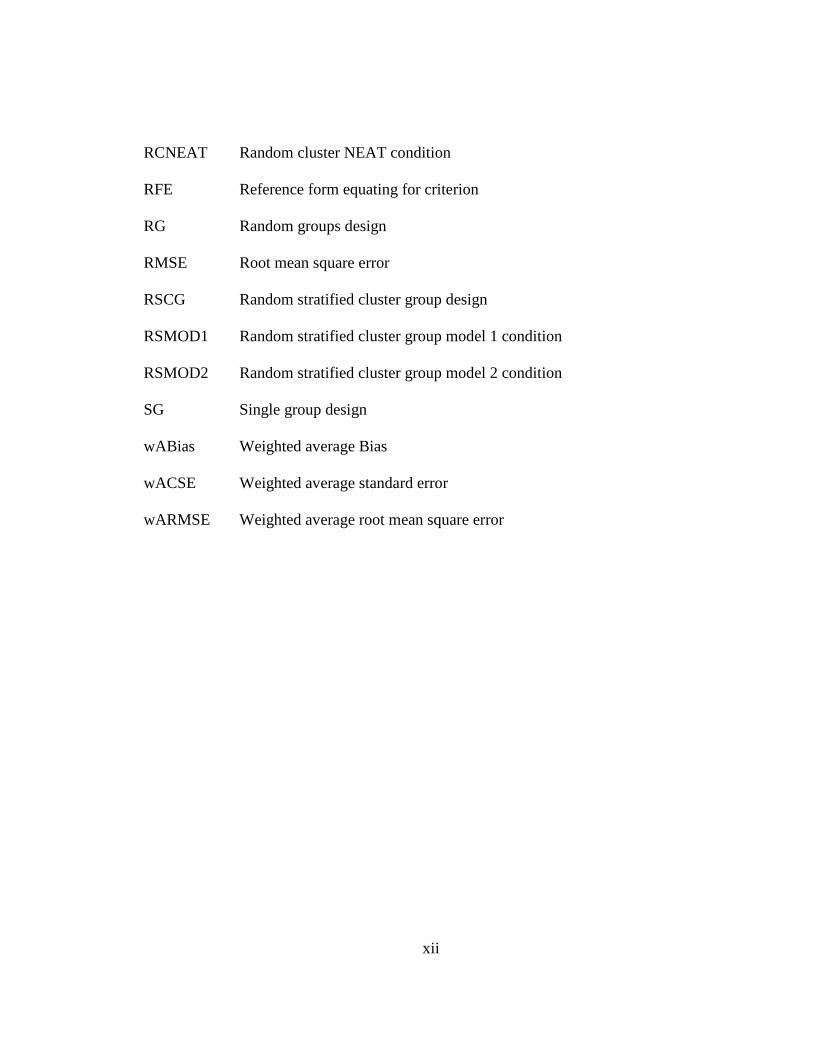
RCNEAT Random cluster NEAT condition
RFE Reference form equating for criterion
RG Random groups design
RMSE Root mean square error
RSCG Random stratified cluster group design
RSMOD1 Random stratified cluster group model 1 condition
RSMOD2 Random stratified cluster group model 2 condition
SG Single group design
wABias Weighted average Bias
wACSE Weighted average standard error
wARMSE Weighted average root mean square error

1
CHAPTER I
INTRODUCTION
1.1. Background
In large scale educational and psychological measurement, test equating and
linking methods are necessary components in testing program that continually produces
new test forms and for which the uses of these tests requires the meaning of the score
scale to be maintained over time (Kane, 2006). A vital objective of large scale
standardized testing is to provide accurate and consistent scales with which examinees’
performance can be compared on different test forms either within the same year, or
across years. These statistical procedures used to place scores of test forms constructed
with the same explicit content and statistical specifications onto common scales are
known as test equating (AERA, APA, NCME, 1999).
The origin of standardized testing and test equating in the USA can be traced back
to the early 1900s from the practical and large scale success of the Army Alpha battery of
assessments. From that point onwards, standardized testing has been established as the
most dominant form of evaluating and improving education particularly in this era of
accountability. Shepard (2006) asserts, “national, state and district-level assessments are
used to collect data to answer the questions of policymakers at some distance from the
classroom” (p. 639). The important meaning of what constitutes standardized assessment
is continuously being redefined by each generation. In the first edition of Educational
2
Measurement published in 1951, the term standardized assessment was entirely
synonymous to objective assessment: Multiple-choice (Brennan, 2006; Lindquist, 1951).
Over the decades, the dominance of multiple-choice (MC) only items in standardized
assessment is steadily dwindling with other item formats such as performance assessment
and process focused assessments gaining prominence. In the most recent publication of
Educational Measurement (Brennan, 2006), several topics are dedicated to item formats
other than multiple-choice. It is once more safe to associate constructed-response item
formats with standardized assessment in this post Thorndike and Lindquist era.
A browse through the literature defines objective items, or MC, as item types in
which the test taker is given a stem followed by possible answer choices from which they
have to choose the one best answer. CR items on the other hand have been identified as
items that require the examinees to generate either part or all of their responses.
The framework adopted from Mctighe and Ferrara (1998) by Ferrara and DeMauro
(2006) has been adopted for this study to define and illustrate the different types of
assessment formats referred to in this study. This framework organizes assessment
approaches in three broad categories of selected responses, which include MC, True-
False, and Matching items:
1. Constructed responses (CR): which is further sub-classified into short
constructed response items—fill in the blanks, short answers, show work,
visual displays (tables and graphs) and performance based tasks—essays,
stories, oral presentations, debates, science lab demonstrations, musical
performances.

3
2. Examiner observes examinee behavior: process focused assessment—
examples include oral questioning, interviews, observation, think-aloud
(Ferrara & DeMauro, 2006).
For the purpose and scope of this study, the term mixed-format tests will be used
to refer to test forms with (a) MC items and (b) CR items consistent with Mctighe and
Ferrara’s (1998) framework. Some examples of large scale standardized assessments that
have adopted mixed-format exams include Advanced Placement (AP) examinations, the
National Assessment of Educational Progress (NAEP), and the Test of English as a
Foreign Language (TOEFL).
The challenge to psychometricians when equating mixed-format test is to
determine how robust current equating methodologies are for both statistical and design
procedures. Currently, there has been very little attention given to this topic in the
equating literature by the standard texts of test equating. The focus of this research is on
the data collection design challenges in equating mixed-format tests. Particularly this
study will experiment with a sampling data collection design under equivalent groups and
will also investigate the effect of dimensionality1 on sampling accuracy.
1.2. Rationale for Research
When multiple forms of the same mixed-format test are used in standardized
assessment with conventional equating designs, the effectiveness to ensure accurate
equating transformation becomes complex.
1 In this dissertation mixed-format dimensionality was not fully evaluated. Instead a dis-attenuated correlation coefficient of less than 1 between the MC and CR sections was used as an indicator of plausible mixed-format dimensionality.

4
1.2.1. Comparability and Equating
After equating, it ought to be a matter of indifference to students, teachers,
administrators and policy makers as to which form of the same test or which items each
examinee sees. Scores for examinees at the same level of proficiency are interchangeable
because there are on a common scale. However, when forms are of mixed-format
construct contamination on composite scores is a likely source of what Luecht and
Camara (2011) referred to as nuisance dimensionality. The use of conventional equating
designs with mixed-format test is likely to result to potential treats of comparability of
scores.
First, in an anchor equating design, the nuisance dimensionality variance on the
composite score greatly impact the effectiveness of the anchor set to adjust for score
differences between groups. Thus the notion of indifference of form administered to
different groups of examinees becomes questionable. Additionally, it is more difficult to
guarantee the stability of the statistical properties of the anchor items between
administrations. The correlation between the anchor and total test varies depending on
which item formats are included in the anchor. Three measurement and practical
limitations associated with the inclusion of CR items in the anchor set are summarized
below.
1. The statistical properties of most CR items are likely to change across forms
as these items may not behave the same for all groups. The reasons could be
attributed to the fact that CR items sample only limited portions of the
construct domain; examinees that were exposed to the topics will perform

5
well and as a result the item statistics will suggest an easy item. Those who
were not exposed to the topics will score poorly and the item statistics will
suggest a very difficult item. The consequence is that the anchor will increase
bias and reduce the overall accuracy of equating.
2. The potentials for differential rater contamination on form difficulty are
greater. The grading of some CR items is associated with considerable degree
of rater subjectivity. Raters in different years are likely to rate the same CR
anchor item differently altering its item statistics in the two groups. Even
within the same test administration rater severity tends to vary. This generally
has an adverse effect on reliability of the anchor set. However, recent
evidence seems to suggest a steady improvement in inter-rater reliability of
CR items as a result of improved rater training. Morgan and Maneckshana
(1996) concluded from empirical evidence that reliability estimates of CR
items have improved from around 0.68 to upper the 0.80. “In 40 years of
constructed response testing, AP has learned much. The current exams are
more reliable than their predecessors. Reader reliability estimates show
continuing improvement at the readings” (p. 18). They attributed the increase
of CR reliability to improved rater training and supervision.
3. The nature of most CR items makes recall and eventual item exposure very
easy. Test security issues of this magnitude threaten the integrity of the entire
assessment and subsequent decisions based on examinee test scores. When
anchor items become exposed, the real differences in ability between the two

6
examinee groups are masked resulting in biased adjustment of scores by the
equating function.
A conventional solution to handle mixed-format test in the NEAT design has been
to use only MC items in the anchor set. The anchor becomes a part-anchor in that only
information from the MC is used to quantify the differences between groups. This
further weakens the effectiveness of the anchor to remove bias in test scores between
groups caused by form difference.
Second, in a random groups design two potential treat of test score comparability
when equating mixed-format test are presented below:
1. When possible, random spiraling of forms does not always guarantee EG in
observational studies. The examinee populations are systematically arranged
into classrooms within schools. Examinees in a classroom are more likely to
be homogenous and not representative of the population. Also it is possible
that examinees differ in their proficiency of different mixed-format
components in a non-random pattern specially when there is evidence of
multi-dimensionality. Thus difference in performance on alternate mixed-
format forms may be due to difference in ability/ proficiency or item
difficulty, with no way to isolated the particular sources of variation.
2. It requires great diligence to assure effective spiraling of test forms especially
in paper administered exams. Test spiraling is most effective with single-
format, MC only tests administered over the computer. Mixed-format test
presents additional challenges to spiraling of forms especially with CR item

7
types such as lab exercises, oral presentations, and listening components (AP
Spanish, TOEFL). Even when effective spiraling can be guaranteed, there is
the security risk of over exposure of all test forms to a small segment of the
population.
In summary, when test are of mixed-format creating an anchor set that is both
content and statistically representative of the whole test has appeared to be a challenging
task. Adding CR items to the anchor set may result in a longer and less representative
sample of the construct domain. This will adversely influence the effectiveness of the
anchor and may also lead to higher cost of test administration and scoring. Also, the
format of some CR items makes them very easy to memorize and a viable candidate for
test-wiseness and item exposure.
On the other hand, the use of MC only items in the anchor set for equating mixed-
format test is not a sustainable solution. Not only does the anchor set become less
representative of the total test forms, it also increases equating bias. Morgan and
Maneckshana (1996) on the equating of mixed-format test with MC only anchor items
affirmed that:
Because the construct measured by the equating items are not representative of all the constructs tested by the exam, the equating error and the potential for scale drift is higher for AP than for testing programs in which equating items and total test measure the same constructs. (p. 18) Finally, in an equivalent groups design framework for mixed-format test, random
spiraling of test forms within classroom is not always feasible given the nature of most
CR tasks. Even in instances where the CR item type allows for random spiraling, this

8
procedure does not always guarantee equivalent samples of examinees are administered
alternate forms.
1.3. Purpose and Research Questions
The purpose of this empirical study is to design and evaluate two predictive
sampling methodologies which will be used to collect data to equate mixed-format tests
under the EG design. Randomization of subjects to treatment conditions [test form] is
most often used to create EG for equating. Unfortunately, ethical and practical
constraints may restrict the use of randomization in most educational studies.
When enough covariates that are highly correlated with the outcome variable
exist, the propensity score through its dimension reduction property provides an efficient
technique to create equivalent groups in observational studies. Haviland, Nagin, and
Rosenbaum (2007) stated that “the propensity score serves to stochastically balance
observed covariates as random assignment of treatments” (p. 248).
In the proposed framework, school performance from previous years is the only
available highly correlated covariate with the outcome measure. Thus the use of
propensity score given the data available is not applicable. The goal of this research is to
create equivalent groups of schools through a sampling framework for equating. The
current design proposes to use previous years’ school performance to create a sampling
matrix of equivalent strata of schools from which random clusters of schools will be
drawn to conduct EG design equating. A second variable of interest in the design is
school size. Although school size is independent of the outcome variable, controlling it

9
in the sampling design is important to ensure comparable sample sizes are drawn within
each stratum.
The premise of the design is that schools that are classified in the same strata
based on the covariate are assumed to be equal in terms of examinee performance. Thus
a random stratified cluster of schools from such frame will result in a good approximation
of randomly equivalent samples of examinees from the population. This modified RG
design will be henceforth referred to as random stratified cluster groups (RSCG) design.
Two experimental sampling models will be analyzed. For the first model (Study
1), a small proportionate sample will be drawn from stratified grid based on previous year
data. Then the subsequent year equipercentile equating relationship between two forms
will be estimated using the RSCG sample and the larger frame. The rationale of this
design is to limit the exposure of one form so it could be reused in the future.
In the second model (Study 2), two random samples of approximately equal sizes
will be drawn from the stratified grid. These two equivalent samples will be used to
estimate the population equating function from two alternate forms administered in the
subsequent year. The rationale is that the two samples are equal to each other and
representative of the larger population from which the sample frame is based. This
model is practical for situations in which scores have to be reported before all test data is
available or to address test malpractice at certain centers.
1.3.1. Research Questions
1. How efficient is a sampling grid stratification design based on previous year
average AP school performance and school size to predict random clusters of

10
school for equating two alternate mixed-format test forms administered during
a subsequent year?
a. Are there differences between model 1 and model 2 in terms of:
i. Conditional equating precision measured by sampling variability of
equated scores?
ii. Conditional equating Bias?
iii. Overall equating precision and accuracy?
b. What are the minimum sample requirements for each model to ensure
acceptable levels of equating precision and accuracy?
2. How does the random stratified cluster group (RSCG) design models compare
to:
a. Random cluster NEAT design with MC only common items?
b. Simple random cluster design?
c. Are there significant differences as measured by equating bias?
d. What is the design effect between the RSCG and NEAT design, and RG
and RSCG design?
e. What is the impact of form difficulty combination in mixed-format test
3. How much precision and accuracy is gained when the stratification framework
is based on more than one year of school aggregated data to predict current
year equivalent cluster of schools?
a. What is the amount of increase in accuracy of predicting equivalent school
strata?

11
b. What is the amount of increase in overall equating error between the two
models?
c. Are these effects consistent across the different AP subjects?
1.4. Overview of Dissertation
Chapter I presents a general introduction of the context and concepts surrounding
this study. Section 1.1 gives a brief background on the need of equating in standardized
assessment. Section 1.2 outlines the most important rationales guiding this research. In
section 1.3 the purpose of this dissertation with detailed research questions are formally
articulated. Finally Section 1.4 presents the road map through this dissertation.
Chapter II presents analyses of existing literature on the theoretical construct and
empirical evidence pertaining to this research. Discussions in this chapter are arranged
under six main sections. Section 2.1 outlines a generic overview of equating designs and
procedures. Section 2.2 provides a summary of data collection designs used in equating.
Section 2.3 provides analyses of the debate on construct equivalence of MC and CR
items. Section 2.4 presents a review of empirical and theoretical literature on equating
mixed-format test. This section if further divided into two sub section: sub section ‘a’
focuses on equating methods in the NEAT design and sub section ‘b’ focuses on aspects
of EG design. Section 2.5 presents an overview of sampling theory as relevant to this
study. The emphasis is to provide basic understanding of the terms used and theoretical
rationale of sampling methods. Section 2.6 reviews various sampling designs with
associated estimation procedures.

12
Chapter III provides a detailed explanation of the methodology used to conduct
this research particularly in addressing the specific research questions. This chapter is
divided into 6 main sections. Section 3.1 presents summary description of the study
methodology. Section 3.2 describes and discusses the rationales used for selecting the
operational AP datasets considered to evaluate the research hypotheses. In Section 3.3,
detailed procedures applied to the operational datasets to create experimental test forms
for equating in a hypothetical situation are explained. Section 3.4 presents a review of
observed score equating procedures used in this research. Section 3.5 presents statistical
evaluation criteria used to summarize equated scores from the various designs and
equating procedures. This section also discusses the various rationales used to establish
the hypothetical equating criteria relationship for the various finite populations. Finally
section 3.6 describes the general procedures and tools adopted to carry out the re-
sampling study.
Chapter IV present overall results for the dissertation. This chapter is organized
into four main sections. Section 4.1 presents summary results of the criterion equating
based on a single group design and equipercentile equating procedure. Section 4.2
presents results for Research Question 1on the differences between RSMOD1 and
RSMOD2. Section 4.3 presents results for Research Question 2 comparing RSMOD1
and RSMOD2 with RCNEAT, RCMOD1, and RCMOD2. Section 4.4 presents results
for Research Question 3 on the effect of equating accuracy when covariates are
aggregating over a two-year period.

13
Chapter V offers discussions and implications of findings presented in Chapter
IV. The discussions in Chapter V are organized in the following order: Section 5.1
presents an overview of the methodology adopted in this research; Section 5.2 presents
the major findings for each research problem; Section 5.3 provides a discussion of the
practical implications of the results; Section 5.4 outlines the limitations of the research
design; and lastly, Section 5.5 offers directions for future research

14
CHAPTER II
LITERATURE REVIEW
In Chapter I, a general summary regarding the rationale and current practices of
test equating was outlined. Arguments were presented to show the limitations of using
the NEAT design to collect data for mixed-format test equating. The most critical of
these limitations were stated as: the difficulty to create a representative and stable anchor
set across forms, issues of differential rater severity on anchor set, and test security issues
with CR anchor sets items. An alternative proposal to use only MC items in the anchor
set was also shown to have enormous practical and theoretical flaws.
The purpose of this study is to explore and evaluate a predictive data collection
model to equate mixed-format test under the EG design. The main goal is to investigate
if the covariates of average school AP score and school size can be used to create an
equivalent group stratification sampling frame. The research hypothesis is that random
cluster samples from a stratified grid can be used to precisely and accurately estimate the
population equating function.
This chapter presents a review of the literature on previous research and theories
surrounding mixed-format equating. A search through the literature on equating reveals
that the issue of mixed-format equating has been scarcely discussed in any of the recent
standard texts (Holland & Dorans, 2006; Kolen & Brennan, 2004; von Davier, 2010; von
Davier, Holland, & Thayer, 2004). However, there are a series of published and

15
unpublished research that has addressed separate aspects of mixed-format test equating.
A review of the most relevant of these studies highlighting their purpose, findings and
limitations are discussed in this chapter. The goal is to identify gaps and weaknesses of
existing research and practices to justify the innovative methodology presented in this
study.
The chapter consists of six main sections. Section 2.1 outlines a generic overview
of equating designs and procedures. Section 2.2 provides a summary of the data
collection designs used in equating. Section 2.3 provides an overview of the fundamental
conceptual issues of construct equivalence in mixed-format test. Section 2.4 reviews key
research on mixed-format test equating. The section is organized into two parts. Part ‘a’
presents research findings of studies on mixed-format test equating under the NEAT
design. Part ‘b’ focuses on the theoretical and methodological rationales to create
equivalent groups in observational studies. Section 2.5 presents an overview of sampling
theory as relevant to this study. The emphasis is to provide basic understanding of the
terms used and theoretical rationale of sampling methods. Section 2.6 reviews various
sampling designs with associated estimation procedures.
2.1. Overview of Equating
Although the exact origin of equating test forms is tenuous, the need for equating
is well documented in the early days of standardized testing in USA. Yoakum and
Yerkes (1920) indicated that the Army Alpha test had five different forms and to avoid
the risk of coaching, several duplicate forms of this examination were made available
(Holland & Dorans, 2006). About two decades later with the development of linear and

16
equipercentile scaling methods, two forms of the College Board’s SAT test were
administered in 1941 and the scores equated (Donlon & Angoff, 1971; Dorans, 2002;
Holland & Dorans, 2006).
Thus, in more technical terms, test equating can be viewed as the process of
controlling statistically for the confounding variable “test form” in the measurement
process (von Davier, 2010). Two other terms which are often associated with equating
are linking and scaling. Dorans and Holland (2000) outlined five requirements for a
scaling or linking study to qualify as an equating: (a) equal construct, (b) equal reliability,
(c) symmetry of the equating function, (d) equity of forms, and (e) population invariance
of the equating function. These requirements are what distinguish equating from weaker
forms of linking and scaling.
In practice, to design an equating study to fulfill all five requirements is very rare.
The combinations of these requirements have been criticized as being too rigid. For
example, Dorans and Holland (2000) followed their outline of the five requirements with
indications of how they “. . . can be criticized as being vague, irrelevant, impractical,
trivial or hopelessly stringent” (p. 283). Livingston (2004) argued the requirements of
equity of forms, and (d) population invariance (e) where unattainable in practice, while
Lord (1980) regarded equity of forms as the most fundamental (Holland & Dorans,
2006). In conclusion, Holland and Dorans (2006) concluded that “regardless of these
differences of opinions, we regard these five requirements as having heuristic value for
addressing the question of whether or not two tests can be, or have been successfully
equated” (p. 194).
17
There are several statistical procedures designed to carry out test equating.
Comprehensive discussions and research on the theoretical guidelines and practical issues
on these equating and linking procedures have been well documented in the literature.
For in depth discussion on equating refer to Lord (1950), Angoff (1971), Petersen et al.
(1989), Dorans and Holland (2000), Von Davier et al. (2004), and Kolen and Brennan
(2004). Holland and Dorans (2006) outlined three factors when attempting to develop
taxonomy of equating methods: common-population versus common-item data collection
designs, observed versus true-score procedures, and linear versus nonlinear methods.
The categorization of observed versus true-score procedures offers a generic way
to classify statistical equating procedures. Under observed score equating (OSE)
methods, the equating transformations are done directly on the raw scores. OSE methods
can be further classified into linear and nonlinear methods. Linear methods map a linear
relationship between scores on the new and reference form. Scores that are of equal
distance from their means in standard deviation units are set equal. Nonlinear methods
on the other hand allow the relationship to be curved. This variation in the slope makes it
possible for the equating relationship to be different for weaker and stronger examinees.
OSE assumes very little about the scores to be equated. These methods do not
directly consider scores of unobservable attributes and as a result they are very appealing
and easy to implement. These practical ease is sometimes viewed by some expert as a
major weakness of OSE. As Braun and Holland (1982) noted
OSE are completely a-theoretical in the sense that they are totally free of any conception (or misconception) of the subject matter of the two tests X and Y . . . we are only preventing from equating a verbal test with a mathematical test by

18
common sense. This is an inherent problem with observed-score equating. (von Davier, 2010, p. 4)
Equipercentile equating is an example of a nonlinear OSE method and is the equating
method used in this research. A detailed description of the equipercentile procedure has
been presented in Chapter III—Methodology.
On the other hand, with true-score equating methods the equating transformations
are done on an estimate of examinees latent ability. There are two main psychometric
models used to estimate examinees true score: classical test theory (CTT) and item
response theory (IRT). True score equating methods were not considered in this study.
The main reasons were to try and replicate operational procedures and also to keep the
scope of the research focused on the data collection design. For detailed descriptions
about true score equating methods and the various psychometric models, see any of the
references on test equating cited earlier.
2.2. Review of Data Collection Designs
A necessary assumption of the statistical procedures for equating is commonality
either among the examinees or the test items. Every equating study begins with a data
collection design. The goal of any data collection design in equating is to create
comparable groups either items or population with which the confounding variance from
test forms can be isolated and adjusted. The equating function adjusts for differences in
test difficulty at the group level. As a result, a key requirement for accurate and fair
equating is that the group of examinees included in the equating study should be
reasonably representative of the examinee population. The implication is that a more

19
representative equating sample will ensure stable equating functions with minimal
sampling error variance for estimating the population parameter.
Unfortunately, the decision and procedures of data collection designs are more
involved as there are practical and statistical specifications guiding most large scale
assessment programs. There are two main approaches to data collection design in
practice. These are the common-population versus common-item categorization in
Holland and Dorans (2006).
The first facet, common-population, has two design options: single groups (SG)
and randomly equivalent groups (RG). Under the SG design, the same sample of
examinees are administered both forms of the test at different time intervals. A
modification of this design to eliminate order effect is called single group with
counterbalancing. An advantage of the SG design is that it requires the smallest sample
size for any given level of precision compared to other designs.
With EG, random or equivalent samples of examinees from the same population
are administered different forms of the test. This can be accomplished through random
spiraling of forms among examinees in the population. When done effectively, test forms
are assigned to randomly equivalent groups of examinees. This design is more practical
than the SG, but does require the largest sample sizes for acceptable error variances
compared to other designs.
A proposed alternative to random spiraling of test forms within classrooms when
mixed-format test are used under the EG design is to create homogenous strata of schools
match on relevant covariates. Then stratify random samples of schools can be drawn

20
from the population stratified frame to estimate the population relationship of mixed-
format alternate forms. This is the framework proposed and evaluated in this research
study.
The second facet of the common-population versus common-item taxonomy
propositions is that the test forms to be equated have to share items in common. The
common-item facet of data collection is referred in the equating literature as either
common item nonequivalent group design (CINEG) Kolen and Brennan (2004) or
nonequivalent groups with anchor test (NEAT) von Davier et al. (2004). This design
relaxes the assumption of same population and allows for test forms administered to
examinees from potentially two different populations to be equated through the anchor-
items. The NEAT design is more flexible than any of the common-population
approaches as it requires only one test form to be administered in each sample and the
two samples could come from different populations (Dorans, Moses, & Eignor, 2010;
Holland & Dorans, 2006).
A key feature in this design is the creation of the anchor set. There are ample
research based recommendations on how to create an anchor set. The most notable is
Angoff’s (1968) guidelines for constructing an anchor set for use in the NEAT design.
Angoff prescribed that the anchor should be a mini version of the test forms being
equated. In addition, others have highlighted that the statistical role of the anchor is to
remove bias rather than to increase precision since it is shorter and less reliable (Dorans
et al., 2010; Holland & Dorans, 2006).

21
The flexibility of equating through the anchor set comes with some assumptions
about missing data and modeling. First, a series of untestable assumptions are made
about examinees performance on items not administered in their group. Second, data for
the NEAT design must be collected and analyzed with great care. Psychometricians have
to continuously evaluate the anchor items to ensure that their statistical properties are the
same in both forms. The correlation between the total test and anchor is also an
important measure of the effectiveness of the anchor in the NEAT design. Because the
NEAT allows the two samples to come from different populations, Holland and Dorans
(2006) cautioned that the information provided by the anchor test becomes even more
critical when the two samples are very different in ability.
Due to the difficulties associated with the creation and maintenance of effective
anchor items, several proposals have been suggested of ways to supplement the
information provided by the anchor test. Wright and Dorans (1993) suggested replacing
the anchor test with a propensity score (Rosenbaum & Rubin, 1983) that includes both
the anchor test and other examinee data. Liou et al. (2001) used a missing data model to
include other variables along with the anchor test score to adjust for sample differences
before equating. Mislevy, Sheehan, and Wingersky (1993) advocated using collateral
information in the absence of anchor test data (Holland & Dorans, 2006).
As highlighted in the various data collection designs, commonality is the vital
component in any equating study. The fundamental difference among various designs is
that the EG design places emphasis on the commonality of examinees, whereas, the
common item design stresses the importance for items to be in common. Rosenbaum
22
(1995) best summed the difference between the common-population versus common-
item designs. He compared it to the difference between experimental designs and
observational studies. The EG design is like a randomize comparison with two treatment
groups. In contrast, the NEAT design is like an observational study with two
nonrandomized study groups that are possibly subject to varying amounts of self-
selection (Dorans et al., 2010).
2.3. Equivalence of MC and CR Formats
MC items have been the most dominant item type in standardized assessment
programs since the practical and large scale success of the Army Alpha test in the early
1900s. The justification for its dominance has been attributed to MC items being
relatively easy to administer, able cover vast content areas, very inexpensive to score, and
efficient to evaluate for psychometric qualities (Bennett, 1993; Wainer & Thissen, 1993).
On the other hand, opponents of large scale standardized assessment claim that MC items
engender “multiple-choice teaching.” Ferrara and Demauro (2006) assert that “MC items
narrow the curriculum objectives that teachers cover and limit approaches to learning and
opportunities to develop skills and thinking that other items encourages” (p. 597).
However, in recent decades, the dominance of MC test has come under scrutiny
particularly from some disciplines where the role of context for some complex
knowledge domain has greater importance than psychometric efficiency. Even during the
early days of “objective testing,” Wood (1923) stated, MC test measure “mere facts or
bits of information” instead of “reasoning capacity, organizing ability” lower order
thinking (Shepard, 2006). On a different note, Bennett (1993) approached the debate
23
between MC versus CR from a unifying platform. He relied on an organizational
framework to represent MC and CR items on a continuum. “This organizational
framework reflects a hypothetical gradation in the constraint exerted on the nature and
extent of the response (but not necessarily on the complexity of the problem-solving
underlying it)” (p. 3). His depiction is that even though MC and CR represent opposite
ends of a continuum, the high degree constraint in MC does not necessarily preclude
construction nor does it eliminate complex problem solving.
Some psychometricians and cognitive experts have adopted a more stringent
approach towards the debate. Robinson (1993) argued that
MC items depend upon recall or recognition of isolated bits of information, rather than requiring the examinee to demonstrate the ability to use information for extended analysis or problem solving. By contrast, CR items permit the examinee to develop an answer that illustrates the knowledge required for an acceptable response. (p. 314)
However, proponents of CR items are not oblivious to the psychometric and economic
cost associated with measuring constructs using these item types.
Lower reliability will make measurements of new construct relatively inaccurate, limiting the ability to generalize performance beyond the administered task and the specific raters grading them. Underlying this low reliability is the larger constellation of skills that these tasks appear to assess. (Bennett, 1993, p. 8) One of the most fundamental requirements of equating is equal constructs. In
order for scores from two tests to be interpreted interchangeably, the test forms have to
measure the same construct. This core equating requirement can be easily assessed when
the test forms are of singular item formats by conducting a dimensionality analysis. With

24
mixed-format test, the evaluation of dimensionality is slightly complicated; the first step
is to be able to disentangle the confounding variance between construct measured and
item format. Theoretical and empirical research evidence on construct equivalence for
mixed-format test is equivocal. Theory appears to be the driving factor in the debate. An
apparent remark in the MC and CR debate is that format affects the meaning of test
scores by restricting the nature of the content and processes that can be measured
(Bennett, 1993; Frederiksen, 1984). But the ‘how’ and ‘when’ are fuzzy in the literature.
Messick (1989) suggested that CR versus MC construct equivalence debate can
be evaluated on both theoretical and empirical grounds. From a theoretical perspective,
critics argue that MC formats: (a) presumes complex skills can be decomposed and
isolated from their applied contexts (Resnick & Resnick, 1990), (b) encourage posing a
limited range of well-structured, algorithmic problems (Gitomer, 1993) and (c) has
engendered a scoring scheme based on a view of learning in which skills and knowledge
are incrementally added (Masters & Mislevy, 1991). “These characterization conflict
with current cognitive theory. Learning is conceptualized as a constructive process in
which new knowledge is not simply added but is integrated into existing structures or
causes those structures to be reconfigured” (Bennett 1993, p. 6). He also noted the above
views are not universally accepted by all cognitive theorists. Some are of the opinion that
MC items can be used to measure the entire domain. Another area of contention among
cognitive theorist is the theoretical role of context in learning and assessment.
So far, empirical research has offered only equivocal evidence regarding the
assertions by cognitive theorist about the equivalence of construct measured by MC and
25
CR items. There are generally two main approaches to research on construct equivalence
for mixed-format test. The first approach is studies that employ stem-equivalents in both
item formats. That is the CR items differ from the MC items only by response format.
These groups of studies suffer from Frederiksen’s (1984, 1990) criticism that “In such
cases, the constructed-responses will measure the same limited skills as the multiple-
choice items” (as cited in Bennett, 1991, p. 77). The second approach is studies that
employ content-equivalent items with independent stems. Rodriguez (2007) further
identified a third approach which he defined as studies that “employs CR items that are
qualitatively different than MC items; they were explicitly written to tap a different
aspect of the content domain or cognitive ability” (p. 164).
Using the stem equivalent approach, Ackerman and Smith (1988) investigated the
similarities between the information provided by direct writing (CR) and indirect writing
(MC). Their rationale was based on theory which suggested that indirect writing and
direct measures of writing ability may in fact be measuring different types of abilities.
The purpose of the study was to provide empirical information regarding the unique skills
and/or abilities measured by each approach. Their methodology was based on a cognitive
model of writing behavior proposed by Hayes and Flower (1980). Hayes and Flower’s
(1980) model provided a loose framework with which writing processes can be
examined. Their mode presupposes that MC items require only the editing and reading
skills (i.e., primarily declarative knowledge) to select an appropriate solution. CR tasks,
on the other hand, demands the procedures of setting goals, generating information,
organizing this information, imposing a grammatical framework, and then reviewing it
26
for possible errors in meaning or structure; thus the task requires both declarative and
procedural knowledge.
Ackerman and Smith (1988) used confirmatory factor analysis (CFA) to analyze
the covariance structure of the various factors associated with different writing models.
Using a sample of 219 10th graders, three instruments were used to collect data for the
study. The first instrument was a MC test that measured six writing abilities—spelling,
capitalization, correct expression, usage, paragraph development and paragraph structure.
The second instrument was a stem-equivalent CR version of the MC items. The third
was an essay in which students were asked to give their opinion on a topic. Reported
reliabilities for the MC test ranged from 0.31 to 0.60 and for the CR the range was .71 to
.88. The generalizability coefficient for the essay score based on six readers ranged from
0.26 to 0.83.
Results from this study suggest that in the area of writing assessment the construct
being measured is a function of the format of the test. Scores from direct and indirect
methods of assessment provided different information. Results also suggest that MC
format can be modified to measure some of the procedural components contained in CR
task without sacrificing the advantage of faster and easier scoring. Evidence from the
CFA showed that the variance structure of the essay score was heavily dominated by
higher-order generation components such as paragraph development and paragraph
structure. Their final recommendation was that both item types may be necessary in
order to reliably measure all the aspects of writing continuum.

27
Bennett, Rock, and Wang (1991) used a design that employs content-equivalent
items with independent stems to assess the construct equivalence between MC and CR
items in College Board Advanced Placement Computer Science (APCS). For their
analyses, two samples each of 1,000 high schools students were randomly drawn from
the 1988 APCS administration. The test consisted of a 50-item MC section and a 5-item
CR section. The MC section was divided into parcels of 10 items each measuring a
separate variable. Each CR item was treated as a separate variable. Confirmatory factor
analysis was used to examine the fit of the covariance structure of two models: a one-
factor and a two-factor model. Factor loadings for both models in all samples were
significant. The loadings for the MC factor were consistently higher than those for the
CR factor. Bennett et al. (1991) concluded that the higher loadings of the MC factor
were possibly due to higher reliability and the fact that the MC items were constructed to
be parallel, causing them to share more variance.
Results from Bennett et al.’s (1991) study suggest that a covariance structure with
just one factor provided the most parsimonious fit of the matrices of correlation
coefficients for the MC and CR variables. The reported factor correlation between the
MC and CR factors was 0.97 for sample 1 and 0.93 for sample 2. They concluded that
“In sum, the evidence presented offers little support for the stereotype of multiple-choice
and free-response formats as measuring substantially different construct” (p. 89). In spite
of their evidential rationale, they cautioned that “there are sound educational reasons for
employing the less efficient format [mixed-format] as some large-scale testing programs,
such as AP have chosen to do” (p. 89).

28
Other measurement experts have not been so subtle when presenting their
arguments based on research evidence. Wainer and Thissen (1993) conducted an
empirical study about the issues with combining scores from MC and CR sections of a
test. They analyzed a number of College Board AP subjects—AP Chemistry, Math,
Music, Biology, European History, and French Language in an empirical research. These
AP subjects used MC and CR items but report a single score. Their hypothesis was that
“The use of a single summary score carries the clear implication that both parts of the
test—multiple-choice and constructed-response—are presumed to measure a single
dimension” (p. 104). They found that the CR section routinely exhibit lower reliability
than the MC section. This was consistent with results based on other AP subjects
(Lukhele et al., 1993; Thissen et al., 1993; Wainer & Thissen, 1993).
Wainer and Thissen (1993) concluded that though there may be evidence of a CR
factor, this factor is so highly correlated with the MC factor that it may be more
efficiently measured using MC items only. As they affirmed, “the contribution to total
error associated with the statistical bias caused by measuring the wrong thing is smaller
than the contribution to error from the unreliability of the constructed-response items” (p.
114). Wainer and Thissen (1993) recommended that before using both item formats the
question must be asked: “What is it that the constructed-response questions are testing
that is not tested by the multiple-choice portion?” (p. 115).
Inspired by motives other than psychometrics, Kennedy and Walstad (1997)
investigated the issue of construct equivalence from what they refer to as an ‘economist
view.’ They wanted to know how many students will be possibly misclassified if the AP
29
CR section in economics was replaced by adding more MC items which are generally
considered economical to administer, score and also more reliable. They conducted a
simulation study with examinee data from the 1991 AP microeconomics and
macroeconomics. They treated the MC and CR sections as if they were independent and
generated two sets of AP scale scores (1-5) from each examinee data.
They evaluated two main hypotheses in the first step of the study. The first
hypothesis was to investigate if there was a significant number of students whose AP
classification based on the MC section of the test were significantly different from their
AP classification based on the CR section. The second hypothesis was related to the first
and further investigated whether preference caused the jump in the number of
classification changes when moving from MC test to the composite test results. Their
initial null hypothesis was the view advocated by Wainer and Thissen’s (1993) about the
actual differences we would expect if the composite scale was from a unidimensional
test. Specifically, the null stated that the CR section measures essentially the same
construct as the MC thus they would expect no difference in the two classifications based
on the separate scores. In their view, acceptance of this null hypothesis would constitute
additional evidence in favor of Wainer and Thissen’s (1993) notion that the use of CR
items in AP exams should be abandoned.
Results from step one, after 1,000 replications, led Wainer and Thissen to
abandon their null hypothesis. They concluded that AP classification based on CR was
significantly different than those based on MC scores. In microeconomics, 8.2% of the
students (329 of 3,996) and in macroeconomics, 7.5% of the students (350 of 4,678) did

30
better on one form of the test than the other. The next step of the simulation was to
examine the number of classification changes in moving from MC score to composite
score for students who had preference on one test format. Kennedy and Walstad (1997)
paid special interest to two new features: the difference between classification errors in
the upward and downward directions and the number of classification changes that
crossed the threshold between category 3 and 4 which most universities used to
determine college credits.
Based on additional manipulation of the data, they concluded that by using both
CR and MC items, misclassification was avoided for 1.2% of the total number of students
in microeconomics and 2.5% of students in macroeconomics. Their conclusion was that
preference does cause misclassification, but of negligible magnitude. For students who
were indifferent of test format, the effect of replacing the CR section with additional MC
questions was modest but statistical significant misclassification at the .01 alpha level.
For their final analyses, Kennedy and Walstad (1997) did a cost benefit analysis
and reported a per misclassification prevention cost of $909 by using CR items. Thus a
total cost of $150,000 for 165 misclassifications caused by using an all MC test. In
response to Wainer and Thissen’s (1993) plea for counterevidence regarding their view
that the CR section of AP test should be replaced by an all MC, Kennedy and Walstad
concluded
. . . admit all the empirical evidence of small misclassification, not everyone agrees these numbers are so small as to justify the abandonment of the CR section. We leave to the reader the task of forming his or her own subjective judgment on this issue. (p. 374)

31
In general, research conclusions on the central issue of construct equivalence
between MC and CR is somewhat divided. Two meta-analyses conducted a decade apart
by Traub (1993) and Rodriguez (2003) has attempted to present comprehensive synthesis
and meaning of research studies that investigated the phenomena of construct equivalent.
The goal of both authors was an attempt to gather relevant evidence from viable studies
addressing the issue of construct equivalence and present a binding argument.
Traub’s (1993) basic premise was that if MC test do not measure precisely the
same characteristics as CR items, then comparisons of difficulty and reliability are
meaningless. In other words, any equating or scaling study will be meaningless as there
will be very little validity evidence to justify score interpretations made from such scale
conversions. In an attempt to address the issue of construct equivalence, Traub searched
the literature for studies that satisfied two requirements—the investigators conducted the
study in such a way that it was possible to assess whether or not the effects on
performance, if any, were consistent with the hypothesis that different abilities are tapped
by MC as opposed to CR items. The research provided information as to the nature of
the observed ability differences, if any. “Few studies satisfy the first of these
requirements and fewer still satisfy both” (p. 30).
Nonetheless, Traub identified and analyzed nine studies. He used a more
restrictive hypothesis of unity of attenuated correlation coefficient between MC and CR
constructs as criterion for evaluation. Traub stated “if a corrected [correlation]
coefficient is not different from unity then we cannot reject the hypothesis that the tests
measure equivalent characteristics” (p. 30). The nine studies selected were classified into
32
two broad categories. The first category was a language task and associated abilities.
This language category was further sub-classified into writing, word knowledge and
reading comprehension. The second category was labeled quantitative task and
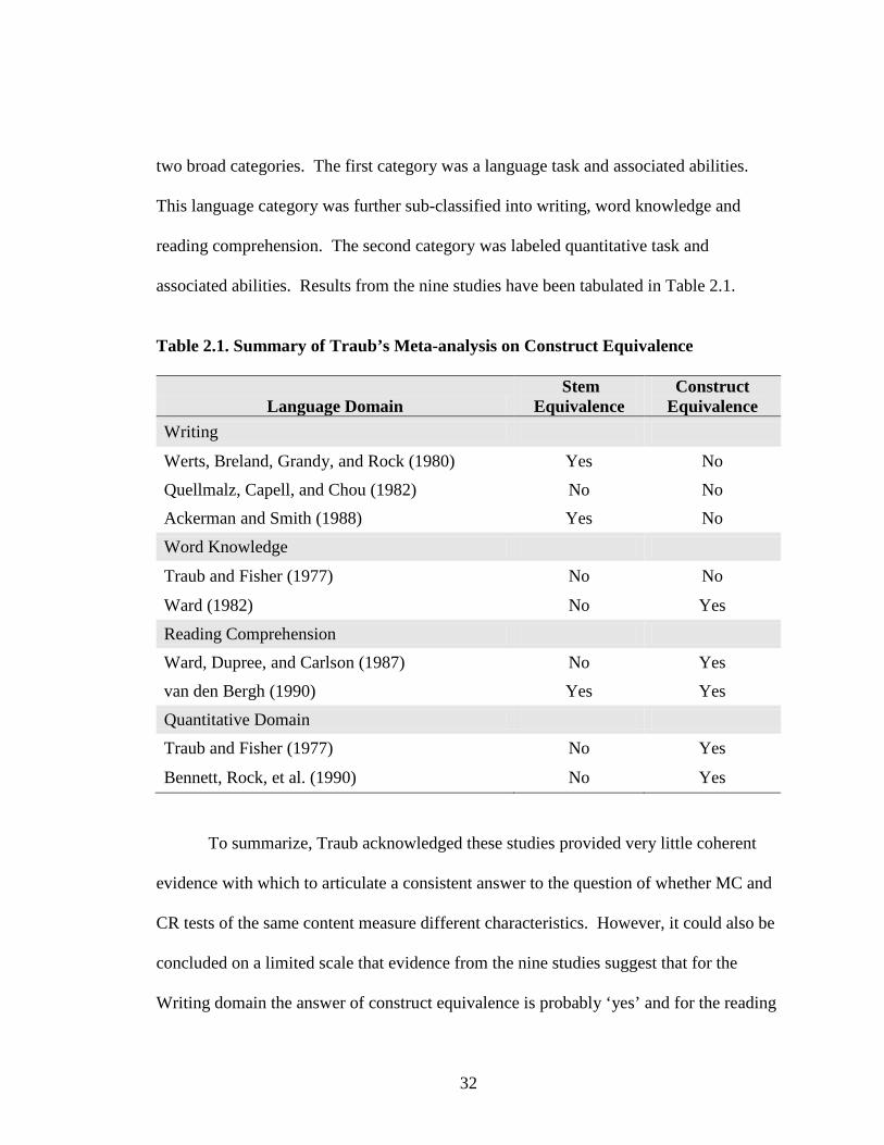
associated abilities. Results from the nine studies have been tabulated in Table 2.1.
Table 2.1. Summary of Traub’s Meta-analysis on Construct Equivalence
Language Domain Stem
Equivalence Construct
Equivalence Writing
Werts, Breland, Grandy, and Rock (1980) Yes No
Quellmalz, Capell, and Chou (1982) No No Ackerman and Smith (1988) Yes No
Word Knowledge
Traub and Fisher (1977) No No
Ward (1982) No Yes
Reading Comprehension Ward, Dupree, and Carlson (1987) No Yes
van den Bergh (1990) Yes Yes
Quantitative Domain Traub and Fisher (1977) No Yes
Bennett, Rock, et al. (1990) No Yes
To summarize, Traub acknowledged these studies provided very little coherent
evidence with which to articulate a consistent answer to the question of whether MC and
CR tests of the same content measure different characteristics. However, it could also be
concluded on a limited scale that evidence from the nine studies suggest that for the
Writing domain the answer of construct equivalence is probably ‘yes’ and for the reading
33
comprehension and quantitative domain the answer is probably ‘no.’ Results from the
word knowledge domain provided contradictory evidence. “An unsurprising corollary
conclusion is that there is no good answer to the question of what it is that is different, if
anything, about the characteristics measured by MC and CR items” (Traub, 1993, p. 38).
Following a similar methodology, Rodriguez (2003) conducted another meta-
analysis on the same central issue of MC and CR construct equivalence. His initial
research question was whether or not the average correlation based on these studies is at
unity. Rodriguez noted that in order to report and interprets a common correlation with a
fair amount of certainty, “we must ask: Are the correlations homogenous across studies?”
(p. 165). Dependent on the outcome of the test of homogeneity of the correlation
coefficient, the next step of the research was to determine whether a random effects
model or a fixed effects model with few explanatory variables was tenable to explain the
differences in correlations across the different studies.
Rodriguez (2003) identified 67 empirical studies between 1925 and 1998 which
addressed the issue of MC and CR construct equivalence. The methodologies employed
in these studies varied—correlational (29), factor analysis and structural equation
modeling (9), analysis of variance models (5), evaluation of item and test statistics (4),
item response theory, and evaluation of overall performance. All 67 studies were
retained for the analysis and correlations were computed or imputed for those studies
which did not report a correlation coefficient or provided information to compute one.
Additionally, all correlations were corrected for attenuation due to measurement error. A
random and fixed effect models were analyzed and results interpreted. Rodriguez’s

34
justification was that random effect model allowed for results to be generalized to
specific tests whose characteristics have not been explicitly studied to date.
Results from a fix effect model confirmed that the average correlation was not
significant across studies; there is substantial heterogeneity in reported correlations.
Rodriguez also found a significant effect on correlation due to design of test items. The
average correlation between MC and CR for stem equivalent item design was 0.92 and
for non-stem equivalent item design the average correlation was 0.85. Item design
characteristics accounted for 23% of the variance in the model whereas there was no
effect due to age of examinees. Even after accounting for these variables in the fixed
effect model, there still remained a significant amount of heterogeneity among study
correlations. In concordance with these results, Rodriguez concluded that a fixed effects
model was untenable at this point.
On the other hand, results from the random effect models offered comparable but
slightly higher estimates of correlation between MC and CR. The average corrected
correlation between MC and CR was estimated at 0.90 with a 95% confidence interval of
(0.86, 0.93). Although this estimate is higher than that of the fixed effect model, the
interval still did not include the restrictive criterion of unity. Other results also indicated
similar patterns of the effect of test design. The average corrected correlation for stem
equivalent forms was 0.94 (CI95%: 0.91, 0.97). Whereas the average corrected correlations
estimates for non-stem equivalent forms were significantly lower at 0.86 (CI95%: 0.81, 0.89).
Amid all this evidence with regard to construct equivalence of item formats,
Rodriguez (2003) concluded that:

35
if we subscribe to the classical definition of trait equivalence described recently by Traub (1993), where true score correlations of unity suggest trait equivalence, such a result was not found. However by accounting for one study-level characteristic, method of item design appears to moderate the level of correlation between the two formats. (p. 179)
2.3.1. Summary
Conclusions from cognitive theorists and empirical research evidences from the
literature on the question of construct equivalence between MC and CR are equivocal.
Majority of the studies reviewed relied on the covariance structure between the two
formats to build an argument for or against construct equivalence. Even with studies that
used factor analysis, the composite factor was not explicitly defined a priori. Messick
(1993) reinforced that what is purported in these studies as evidence of construct variance
is merely what Loevinger (1957) and Campbell and Fiske (1959) had defined as method
variance. Messick (1993) reaffirmed,
Thus every measure basically consists of a construct-method unit. As a consequence, we need to distinguish, at least conceptually, those aspects of performance that are reflective of the construct from those that are responsive to the method—or in the present context from those that are differently responsive to different method. (p. 66) Lessons learnt from the literature are that the debate on construct equivalence of
mixed-format test is mostly philosophical. Psychometricians ought to first define the
intended construct to be measured, then design items using appropriate formats to
measure all aspects of the construct. Rodriguez (2003) also noted, “. . . the choice of
item formats are informed by these results but also depends on cost as well as political
and other considerations” (p. 180). Item format does not inherently measure different

36
constructs. Pos-hoc exploratory psychometric analyses on dimensionality as
demonstrated in some of the studies reviewed only adds to the inconsistencies.
2.4. Research on Mixed-Format Equating
Measurement experts are continuously evaluating new options in search of the
best practices for handling mixed-format test equating. Mixed-format tests are unique in
that there is a continuum of item types (see Chapter I) that can be combined to create a
mixed-format test. Each of these combinations adds distinctive challenges into the
measurement cycle. Thus a best practice approach for all types of mixed-format test is
impractical. Comprehensive review of research evidence on mixed-format test is
somewhat specialized to particular programs and associated item types. The scope of
research evidence reviewed in this section will focus primarily on the data collection
design of the equating process. Specific issues dealing with relationships among item
types such as dimensionality concerns, accuracy of different equating procedures are not
the focus of this review.
Relevant empirical studies which have looked into issues of mixed-format
equating are organized into two broad categories based on the data collection design
methodology—NEAT and RG. Contributions provided by these studies will be presented
and their implications highlighted. The review of the current literature will expose the
need for the proposed research. It will also provide theoretical evidence for the
innovative methodology proposed for mixed-format equating.

37
2.4.1. Mixed-Format Equating—NEAT Design
The NEAT design is the most dominant data collection design in large scale
testing programs where equating is an integral component of the testing process. The
NEAT design has been stated to offer a flexible data collection plan for equating test
forms with an incomplete data collection plan using the anchor set as the link. Myriads
of research evidence are available in the literature about the appropriateness of using
NEAT designs in equating test forms with predominantly MC items. When test forms
are composed of all MC items, a representative anchor—statistical and content—is
created to match the whole test as prescribed by Angoff (1968). Additionally, Dorans et
al. (2010) outlined that the most important properties of the anchor tests are its stability
over occasions when it is used and its high correlation with the scores on the two tests
being equated. When the anchor test meets these three properties, research has confirmed
that it can be used with efficacy to equate test forms with minimal bias under the NEAT
design.
However, when the test forms to be equated are of mixed-format, meeting these
properties for good anchor sets becomes very difficult. Tate (1999, 2000, 2003)
conducted a series a simulation studies in which among other issues investigated
problems associated with using the NEAT design for linking mixed-format tests using
IRT. Tate’s basic premise was that most of the traditional linking methodologies were
developed to link test with MC items. Thus the applications of these same linking
procedures to test containing CR items would not be appropriate under certain
circumstances.

38
In particular, when the item “responses” are ratings from one or more judges and the severity of the rating team may change from year to year, the common item/rating team parameter from the calibrations for the two years may be different for two reasons: a year to year change in student ability and a change in the rating team severity. (Tate, 2000, p. 330)
He argued, in such scenarios, the anchor test which is supposed to adjust for differences
in ability between the two groups will be contaminated by the changes in rater severity
and or item difficulty and as a result lead to bias linking.
In order to minimize bias caused by differential rater severity, Tate (1999)
proposed an additional linking study where a random selection of previous year
examinees CR section are rescored by the current year raters. This procedure is widely
referred in the equating literature as trend scoring. Using simulation studies he
investigated the performance of two proposed modification to traditional equating
methods: extended mean and sigma approach, and the graded response model extension
of the Stocking and Lord Procedure.
Based on results from these studies, Tate (1999, 2000, 2003) concluded that the
modified IRT linking methods demonstrated an increase in precision over traditional
methods for test with mixed-format. Results also suggested that the use of MC only
items as anchors for mixed-format test will lead to serious linking bias especially when
there are evidences of multidimensionality across item types.
Regarding the issue of changes in rater severity across years, Fitzpatrick, Ercikan,
Yen, and Ferrara (1998) also conducted a study to assess the consistency of raters over
three years in: reading, writing, language usage, mathematics, science, and social science.
One purpose of the Fitzpatrick et al. (1998) study was to provide evidence on the
39
consistency of scores obtained from raters on the same students in different test years.
They also examined the consistency across grade levels. Their methodology consisted of
trend scored CR items in which a random sample of examinees responses were
systematically scored by trained raters in two different test years. This study was part of
the general operational equating plan.
Using evaluation criteria of absolute standardized mean difference, standard
deviation ratio and percentage agreement they reached several findings. First, overall
consistency between two groups of raters was higher when rater training and rubric was
consistent. Second, there was noticeable trend in rater consistency across the different
content areas and grade levels. Rater consistency was highest for mathematics content
area and language arts demonstrated the least consistency. In terms of grade level, grade
8 scores tended to be the most consistent with grade 3 scores being the least consistent.
Analyses from their research lead them to conclude that raters used in different
test years will demonstrate inconsistency in their ratings by an average of one-tenth to
two tenth standard deviation. The implication based on their scenario was that 9% of
fifth graders would have been inaccurately classified into proficiency categories had
these scores not been adjusted for rater severity. Based on knowledge gain from
experience and from the study, Fitzpatrick et al. (1998) recommended that:
Raters are likely to become more consistent when they are using scoring rules that refer to observable qualities in students’ responses than when they are using rules requiring that abstract qualities be inferred from students’ response. (p. 207)
40
The implication of the Tate (1999, 2000, 2003) and Fitzpatrick et al. (1998)
studies are that the transition of the NEAT design from test with MC items to mixed-
format test requires additional steps in order for test scores to be comparable. In addition
to untestable assumptions regarding missing data in the NEAT design there is another
main measurement concern. The statistical power of the anchor for mixed-format test to
accurately quantify the ability differences between the two groups is further weaken by
the apparent confounding variance caused by using different raters. The interaction
between rater and item difficulty needs to be isolated and addressed. Trend scoring has
been proposed to alleviate some of this confounding variance. Although research
evidence on the success of trend scoring is promising, more research evidence is still
required. And as Fitzpatrick et al. (1998) showed, the accuracy of trend scoring vary
across different content areas.
On the practical side, the planning and implementation of a trend study adds to
the complexity of the data collection design. If CR items have changed in difficulty or
removed from the anchor set, accounting for such inconsistencies in a trend study when
training raters and administering new test forms could prove to be very challenging.
In the context of classical equating, Kim, Walker, and McHale (2010) compared
four data collection models under the NEAT and EG designs to determine the most
effective procedure for equating mixed-format test. The three equating designs
investigated under the NEAT design were: MC only anchor, MC and CR anchor, and MC
and trend scored CR anchor item. The fourth design was EG in which the two forms had
no anchor items and were randomly spiraled to examinees. Their research focused on

41
two main questions: (a) Which equating design is the most effective for linking CR
items? and (b) What anchor test composition works best?
To address these questions the authors used a re-sampling methodology in which
two forms of an operational test were used to create two experimental test forms with
anchor items. Evaluation criteria of standard error and bias were used to assess the
effectiveness of the various designs. Summary results from the study suggested that EG
design provided the most effective metric with which to equate mixed-format test. The
second best design was MC and trend scored CR anchor item.
Kim et al. (2010) concluded that their results were consistent with other studies
which showed that the use of MC anchors only or MC and CR anchor with no trend
scoring for equating mixed-format test using the NEAT design would result to large
equating bias. Also, the difference as measured by bias between the EG design and MC
with trend scored CR anchor was not significant. Their final recommendation was that it
is up to practitioners to weigh the strength against the limitations of each design then
decide which is appropriate for their program.
In a similar context, Rotou, Walker, and Dorans (2011) investigated the effect of
the structure of anchor sets for mixed-format test under the NEAT design. They
articulated their research goal as an attempt to fully understand how the equating
conversion will be affected when the anchor set does not fully meet the content, statistical
and dimensionality properties of mixed-format test forms. They studied five anchor set
conditions: (a) The anchor was comprised of a set of representative MC items only; (b)
The anchor set was comprised of CR items only; (c) The anchor was comprised of a set

42
of representative MC items and one CR item; (d) The anchor set was comprised of CR
items and two CR items; and (e) The anchor set was comprised of CR items and all CR
items.
Rotou et al. (2011) used data from an operational test in two content areas. Using
evidence from the correlation coefficient between the MC and CR section they
categorized each of the two operational tests as either one-dimensional or
multidimensional. A simulation study was designed in which the operational test data
was used to create two sets of experimental sample test forms. In the first set, two EG
samples of 5,000 examinees were selected and conditioned to have a standardized group
difference of 0.0 based on composite score. For the second set, the standardized group
difference was set to 0.10 to create a NEAT design. Levine observed score equating was
used to equate the test scores from each set: EG with anchor items, and NEAT. The
identity equating function was set as the criterion to estimate conditional bias, and
precision was assessed using standard error.
Analyses from their study with respect to the structure of the anchor set led them
to conclude that content and statistical representativeness of anchor set does affect the
amount of equating accuracy as measured by bias. The amount of improvement in terms
of bias reduction from an anchor set with MC only to a set that included one CR items
was much more noticeable for the multidimensional condition than for the one-
dimensional condition. Overall, for all conditions with MC anchor, when more CR items
were added to the anchor set the quality of equating accuracy and precision improved.
They attributed this improvement in equating quality to the fact that the addition of more

43
CR items resulted in more content coverage by the anchor set which in turn improved the
correlation between the anchor and total test score.
Similar research studies by Hagge and Kolen (2011), unpublished dissertations by
Hagge (2010) and Cao (2008) also arrived at similar findings with regard to the
representativeness of common items for mixed-format equating. Hagge and Kolen
(2011), in a paper presentated at the NCME annual conference, among other factors were
interested to understand how the characteristics of mixed-format test might adversely
impact equating under the NEAT design. Examinee test data from a single
administration of AP Spanish was used in a resampling study to provide answers to these
specific questions:
1. What is the impact on equated scores when examinees on one mixed-format
test form are higher in proficiency than examinees on the other mixed-format
test form?
2. When one type of item format (i.e., MC or CR) is relatively more difficult for
examinees taking one form as compared to examinees taking another form,
how are the resulting equated scores impacted?
3. How much do equated scores vary across equating methods?
4. How does the composition of the common items impact equated scores?
Summary results from Hagge and Kolen (2011) showed an inverse relation
between the proficiency gap of the two groups and accuracy of equating mixed-format
test using the NEAT design. For Research Question (II) their conclusions are in
agreement with findings previously discussed. There was evidence of increased bias

44
when examinees of the two groups perform differentially on the MC and CR section and
only MC items were used as common items. With regard to Research Question (IV) they
too found mixed result regarding the reduction in bias. When the correlation between
MC and CR section was high the amount of bias introduced by using only MC common
item was negligible. However, when the correlation was low, including CR items to the
anchor set helped to significantly reduce bias and improved the accuracy of the equating
conversion.
2.4.2. Summary Implications
Research evidence highlighted from studies reviewed all point to several general
conclusions regarding the effectiveness of equating mixed-format test using the NEAT
design.
First, with regard to the contention of whether we can use MC only anchor items
to equate mixed-format test, research evidence recommends shying away from such
practice. Evidence from studies reviewed showed that when the anchor set was made up
of only MC items, equating bias was highest. However, Rotou et al. (2011) found
evidence of lower bias when the dis-attenuated correlation between the MC and CR
scales was close to unity and the anchor set was made up of only MC items.
Second, research evidence showed that simply including the appropriate
combination of MC and CR items in the anchor set is not enough to guarantee accurate
equating conversions. Adjustment must be made regarding rater severity from one test
administration to the next. The success of the NEAT design depends to a greater extent
on the successfully implementation of the common item CR trend scored linking.

45
Finally, it can be deduced from this handful of studies that the NEAT design does
not seem to offer the best avenue for equating mixed-format test. There are several
uncertainties such as the effect of different types of CR items on the anchor set. A
parsimonious EG data collection design that involved the spiraling of test forms to
random sample of examinees produced comparable estimates of bias as the complex
NEAT design with MC and trend scored CR items. The unexploited potentials of using
EG design to equate mixed-format test, thereby, negating the need for an anchor set is
what this study aims to exploit.
2.4.3. Propensity Score and RG Design
A potential drawback of research presented this far on mixed-format equating is
the over reliance on the NEAT design as the de facto data collection model for equating.
An underlying assumption in these studies is that the NEAT design can be used to
demonstrate acceptable levels of accuracy for equating mixed-format test forms provided
the correct adjustments are made to the anchor set. The reality is that unlike in MC test
were the main factors considered when selecting the anchor set are item difficulty and
content representativeness; the list is longer for mixed-format test. In addition to
difficulty and content specifications, test developers have to take into consideration the
types of CR items included in the test, the correlation between the various item formats,
dimensionality assessments of the various item formats, scoring procedures and rater
effects.
A viable alternative around the intricate process of assembling anchor sets for
mixed-format test can be accomplished by creating equivalent groups of examinees with
46
which the confounding effect of test form can be adequately addressed without the need
for an anchor set. This is what a RG data collection design accomplishes.
),|1()( iiii xXWprxe === (2.1)
where e(xi) is the conditional binary probability, W is a dichotomous variable indicating
group membership and Xi is a vector of observed covariates.
Guo and Fraser (2010), in their in depth analysis of propensity score clearly
articulated the counterfactual frameworks and assumptions which guide the estimation of
treatment effects. They showed that counterfactuals have been established in science as
the main framework to investigate causality.
Counterfactual is a potential outcome . . . Thus for a participant in the treatment condition, a counterfactual is the potential outcome under the condition of control; for a participant in the control condition, a counterfactual is the potential outcome under the condition of treatment. Which means the counterfactual is not observed in real data. Indeed it is a missing value. (p. 24) Thus in scientific studies randomization is used to balance the treatment and
control groups so that the counterfactual can be estimated by comparing the average
outcome between treatment and control participants. The key factor in the estimate of
treatment effect is the effectiveness of randomization to balance the groups on all other
covariates. Following this logic, Rubin (1974) extended the counterfactual framework to
observational studies in what is referred to as the Neyman-Rubin framework. Guo and
Fraser (2010) pointed that:

47
The Neyman-Rubin counterfactual framework is mainly a useful tool for the statistical exploration of causal effects. However, by no means does this framework exclude the importance of using substantive theories to guide causal inferences. Identifying an appropriate set of covariates and choosing an appropriate model for data analysis are primarily tasks of developing theories based on prior studies in the substantive area. (p. 30)
Test equating can also be viewed as solving a counterfactual with two steps. In
step one; the goal is to determine the potential outcome had the each group been
administered both test forms. Step two then balances for the confoundedness caused by
test forms in both groups. When randomization is applied to an observational study, the
critical assumption of ignorable treatment assignment is wholly violated and as a result
the treatment and control groups varied systematically introducing bias in the average
treatment effect. Rosenbaum and Rubin (1983) argue that in such circumstances
comparison of treatment effect is at best speculative.
Rosenbaum and Rubin (1983) demonstrated that in order for the assumption of
ignorable treatment assignment to hold in observational studies, assignment to either
treatment or control group has to be independent of the potential outcomes if observable
covariates are held constant. Using Dawid’s (1976) notation, Rosenbaum and Rubin
(1983) expressed this assumption as:
),(| xbzx ⊥ (2.2)
where X are the observed covariate, Z is group assignment and b(x) is a balancing score.
Guo and Fraser (2010) further explained that the delineation of the ignorable treatment
assignment in the propensity model implies
48
Therefore, for observations with the same propensity score, the distribution of covariates should be the same across the treated and control groups. Further, this property means that, conditional on the propensity score, each participant has the same probability of assignment to treatment, as in randomized experiment. (p. 133)
In summary, the use of propensity score offers a series of flexible but measurable
metric to create equivalent groups in non-experimental study conditions. This
methodology can be extended to address the confounds associated with test equating
without the need for anchor set or requiring examinees to take both test forms. As
Rosenbaum and Rubin (1983) demonstrated, if the ‘right’ covariates exist, then
propensity scores will produce equivalent samples. The unbiased treatment effect
(different test forms and raters) can then be estimated as the difference in performance
between the two groups.
The greatest practical limitation of propensity scores methodology in
observational studies as highlighted by Peikes, Moreno, and Orzol (2008) is the
identification of the right covariates. Misuses of propensity scores are common when
researchers have attempted to create EG using a series of demographic or limited number
of covariates that have very little effect on the outcome variable—test score. This
generally has resulted in a rash conclusion that propensity scores cannot be used to
produce unbiased estimates of the average treatment effect in observational studies.
2.5. Sampling Designs and Variance Estimation
This section presents a general overview of sample design as applicable to this
research. The interdisciplinary field of sample design can be operationalized as focusing
on two main aspects: a selection process and an estimation process. The review

49
presented in this section has two main purposes. First, is to provide understanding of key
concepts of sample design and provide theoretical rationale of their applicability to
observational studies. The second purpose is to familiarize the reader with relevant
sample design terminologies and procedures that will be used in this study. This section
is organized into a systematic classification of the main components associated with
sampling: overview of sampling theory, and definition of technical terms.
2.5.1. Overview of Sampling Theory
Sampling theory provides a framework with which researchers can effectively
extrapolate particular aspects about the entire population from data collected on a small
representative group. Jaeger (1984) identified two types of generalizations involved with
sampling—statistical and substantive generalization. Statistical generalizations are
generally prone to two types of errors: ‘bias error’ and ‘standard error.’ Kish (1965)
defined bias error as systematic errors that affect any sample taken under a specified
survey design with the same constant error. Bias errors are estimated directly by taking
the difference between the average sample estimate and the ‘true’ population value. The
concept of ‘true’ population value is generally tenuous as the concept population is very
relative. For unbiased samples bias error is very close to zero. The general tendency is
that for well-designed samples bias error tends to diminish with increasing sample size
(Kish, 1965).
Standard errors, on the other hand, provide a measure of the average random
fluctuation of the estimated sample statistics for replicated samples. Different sampling
designs would result in different standard error estimates, and choosing the design with

50
the smallest error is the principal aim of sampling designs (Kish, 1965). A widely
accepted model in sampling theory combines bias error and standard error into ‘Total
Error’ or in sampling terminology root mean square error (RMSE) or mean square error
(MSE):
RMSE = 22var Bias+ (2.3) MSE = Var2 + Bias2 (2.4)
Though the concept of total error is routinely used to evaluate sample estimates,
some statisticians argue that bias errors are not a sampling problem and as such should be
separated from sampling error. The terms precision and accuracy are used in the
literature to separate the effects of error variance and bias. Kish (1965) asserts these
arguments are analogous to those between the concepts of reliability and validity. A
precise sample estimate has low error variance (high reliability). An accurate estimate
has low bias (validity). The concepts of precision and accuracy of sample estimates are
equally important considerations. Precision of sample estimate is measureable and can
be quantified using statistical models. On the other hand, the evaluation of accuracy of
sample estimates like the concept of validity involves attributes that go beyond statistical
models. A balanced approach is always ideal.
Substantive generalization of results from a sample to the population has been
described by Jaeger (1984) to be even more difficult. It involves a series of assumptions
ranging from validity issues to accuracy of data collection techniques and instruments.
51
The goal of an effective sampling study is to minimize the errors associated with
statistical generalization so that substantive generalization can be feasible.
2.5.2. Definition of Technical Terms
Definitions of selected technical terms are provided below to enhance
understanding of the sampling designs discussed in this study. There is an exhaustive list
of sampling jargon, but only terms that directly apply to this research are defined. The
definitions and notations presented below have been adapted from Kish’s (1965) Survey
Sampling.
2.5.2.1. Population. The population is the aggregate of the elements, and the
elements are the basic units that comprise and define the population. Kish suggested the
population must be defined in terms of: content, units, extent, and time. Kish also
cautions that universe is not necessarily synonymous to population. “A universe denotes
a hypothetical infinite set of elements generated by a theoretical model” (p. 7). In certain
designs to improve selection, the population is divided into subpopulations called strata
with homogenous characteristics.
2.5.2.2. Sampling frame. Sampling frame is the actual totality of elements in the
target population that have a greater than zero probability of being selected into a sample.
For example, if the population is identified as high schools in North Carolina; the
sampling frame is the list of high school names from which the selection is done. In most
sampling studies the sampling frame is different from the population. Groves et al.
(2004) referred to this difference as coverage error. They identified two types of
coverage errors: undercoverage and overcoverage. ‘Undercoverage error’ occurs when
52
the sampling frame does not include all the elements from the population. ‘Overcoverage
error’ occurs when the sampling frame includes elements not defined in the population.
2.5.2.3. Elements. Elements are units for which information is sought; they are
the individuals, the elementary units comprising the population about which inferences
are to be drawn. These are the units of analysis. Sample units vary by selection methods.
For simple random sampling these are individual observation such as students. In cluster
sampling units could be classroom, schools or even school districts depending on the
population.
2.5.2.4. Probability sampling. Through probability sampling, every element in
the sampling frame has a known nonzero probability of being selected. This is usually
done through some mechanical operation of randomization. The use of a randomized
mechanism allows statisticians to make inference about the population from a sample
entirely through statistical methods without any assumption about population distribution.
Kish (1965) emphasized that “Probability samples are usually designed to be measurable;
that is, designed that statistical inferences to population values can be based on measures
of variability usually standard errors computed from the sample data” (p. 20). Equal
probability selection method (epsem) is the idealized probability approach. Other
probability selection methods are deviations from epsem caused by peculiar properties in
the sampling frame.
2.5.2.5. Finite population correction (fpc). Finite population correction (fpc) is
a statistical adjustment included in the error variance estimation procedure when samples
53
are selected without replacement from a fixed frame. Computationally, fpc is expressed
as:
fpc = 1- f, (2.5)
where f = n/N the fraction of units selected into sample of size (n) from all the elements
in the frame (N).
The fpc is used as a multiplier to the variance estimate from the sample. For
larger samples, fpc is significantly less than 1 and tend to decrease the sampling variance
term.
2.5.3. Variance Estimation
The basic structure of a sampling design has two main components. The first is
the selection procedure which defines the rules by which data are collected. The second
component is an estimation procedure for computing standard error of sample statistics.
The selection procedure is normally done either with replacement or without
replacement. For sampling with replacement, each population element can be selected in
the sample more than once. When the sample is selected without replacement, an
element can only be selected once from the frame population. Given the scope of the
research, three sampling designs are discussed in this section: simple random (SRS),
cluster sampling (CS) and stratified cluster sampling (SCS). The selection and variance
estimation procedures for each of these sampling designs are discussed in greater
detailed.

54
2.5.3.1. Simple random sampling. SRS is the process by which ‘n’ elements are
selected from a random set of N units (frame population) where each of the ‘n’ elements
has an equal probability of being selected from the N units. In SRS, the unit of selection
is individual elements. Kish (1965) suggested that the term SRS be applied only when
sampling is without replacement and unrestricted sampling when the sampling is done
with replacement. Kish also highlighted that SRS is a special type of epsem because
elements have the same fixed selection probability of n/N. SRS is the standard sampling
design with generally highest level of precision for a given sample size compared to other
designs.
Even though SRS possesses tremendous theoretical and statistical advantages, it is
hardly used in practical educational and social sciences studies in its purest form. An
obvious reason is that most sampling frames have irregular properties such as
disproportionate allocation of key variables. In spite of its practical shortcomings, Kish
(1965) outlined four important reasons for the importance of SRS in sampling theory.
First, because of its simple mathematical properties most statistical theories assume
simple random selection of elements. Second, all probability selection may be viewed as
a restriction on SRS. Third, the relatively simple SRS computations are often used on
data obtained by more complex selection. Fourth, SRS computations are often used as a
convenient base, and then adjusted for the design effect of the sample design actually
used.
The estimation procedure of sampling error for the SRS follows standard
notations of variance and standard error. Assuming replicated samples are selected using

55
SRS (sampling without replacement) from a fixed population the expected estimate for
variable yi over all samples is obtained by
,1∑=n
iii y
ny
(2.6)
where yi is the ith item score, n is the number of replications.
The variance of the mean estimate for SRS is obtained by
,)1()var(
2
nsfyi −=
(2.7)
where
−
−= ∑ ∑n
i
ii n
yy
ns
222 )(
11 and
Nnf = and )var()( ii yyse = (2.8)
As illustrated by equations 2.6–2.8, the standard error for SRS is inversely related to the
sample size. Larger ‘n’ leads to smaller standard error estimates and these translate to a
narrower confidence band for the estimated statistics.
Obtaining equivalent groups for equating can be theoretically accomplished
through SRS. Unfortunately, SRS of individual elements as the primary selection unit is
not suitable for most test designs and content area where elements exist in predefined
systematic clusters and share common characteristics. Classrooms are likely to be
comprised of homogenous units thereby, random selection of examinees or random

56
spiraling of test forms does not necessarily guarantee EG. These and other practical
issues can be addressed through alternative sampling designs.
2.5.3.2. Cluster sampling. Cluster sampling provides a convenient and more
practical alternative to sampling when the sample elements already exist in clusters such
as classrooms. Kish (1965) defines cluster sampling as a method of selection in which
the sampling unit, unit of selection contains more than one population element. A key
rule regarding cluster membership is that each element of the population can only be in
one unit. EPSEM can be used to select clusters. If clusters are of equal size, the planning
and implementation of cluster sampling is straight forward—accurate sample sizes,
number of clusters needed and cost involved can be predicted.
However, the reality is that clusters are often of unequal sizes. This makes
planning and variance estimation procedures even more complicated. Kish (1965)
outlined three problems with selecting unequal clusters. First, the size of the sample
becomes a random variable, depending on the chance of selection of larger or smaller
clusters. Second, ratio means are used in place of simple mean and though it provides
practical estimates, it is not an unbiased estimate of population mean. Third practical
variance formulas are not unbiased estimates of the true variance.
The estimation of ratio mean for any number of unequal clusters is denoted by:
α
α
α yax
xax
yra
∑==1
, and ,α
αα x
yy = (2.9)

57
where r represents the ratio mean of the two random variables y (test scores) and x
(school size), α represent a cluster total and x/a is the average cluster size. In the above
notation, the means are weighted with their relative sizes.
The variance estimation involves the sum of three separate variance terms.
]2[1)var( 222
2 yxxy rssrsax
fr −+−
= (2.10)
This can be expanded as
−−
−+
−
−−
= ∑∑∑ ayxxyr
axxr
ayy
aa
xfr αααα 2
11)var(
222
22
2
(2.11)
Kish (1965) proved the terms (y2 + r2x2 -2ryx=0) because r= y/x for cluster
samples and the variance formula simplifies to
∑∑ −
−−
= ]2[1
1)var( 22 ααα xyry
aa
xfr
(2.12)
Like the variance for SRS which has just one variance component and a factor of
sample size, the variance for cluster samples have three additional sources of variations—
within cluster, between cluster variance, plus the covariance of the random measurement
outcome variable and sample size. Low within cluster variance (high degree of
homogeneity) is likely to result to higher between cluster variance and this will have a
magnifying effect on the overall variance estimates. The effect of clustering has been
reported to almost triple the variance term compared to SRS (Groves et al., 2004). Jaeger
58
(1984) alluded that the simplicity and savings benefits of cluster sampling carry huge
measurement cost.
Student compositions within schools are often systematically based on a
combination of socio-economic variables and previous performance. Between schools
homogeneity can also be attributed to teacher effect effects, educational leadership,
school climate and a myriad of other factors that might be related to aggregate
performance with each school. High homogeneity within schools implies that more
clusters are needed for small gain in precision. Kish (1965) recommended that to control
the effect of homogeneity of clusters, a valuable rule of thumb is to be sure the standard
error of cluster size is less than 0.20. Larger homogenous clusters tend to magnify
overall variance estimate.
2.5.3.3. Stratified cluster sampling. Stratified sampling is generally
recommended when sampling clusters to reduce overall variance estimates. This is
accomplished by grouping clusters with similar characteristics into non-overlapping
stratum. Jaeger (1984) asserted that “the primary benefit afforded by stratified sampling
is increased statistical efficiency” (p. 67). He also added that wise stratification before
sampling avoids selection of undesirable samples that might be selected through other
procedures. Sampling stratified clusters leads to two general benefits when appropriately
implemented. The first advantage of stratified cluster sampling is that cost of sampling is
reduced by sampling clusters when the per unit cost of sampling individual elements is
greater. Second, efficiency of the estimation is improved by the use of appropriate
stratifying variables. The goal is to use classification variables which lead to

59
homogenous grouping of clusters based on the measurement variable. Hansen et al.
(1953, p. 229) suggested the use of classification variables that are highly correlated with
the sampling variable:
The most effective variable on which to stratify would be the characteristic to be measured; and since in practice this is not feasible, stratification on the most highly correlated data available will lead to the greatest reduction in variance. (as cited in Jaeger, 1984, p. 91) Additionally, Kish asserted that cluster samples are generally selected with
stratification because stratification has more advantages for clustering than for element
samples. He also recommended that one way to control for total sample size when
sampling unequal clusters is to stratify on cluster size. Kish (1965) reported that “if the
distribution of cluster sizes is rectangular, creating H strata can reduce the standard
deviation of cluster sizes within strata by the factor H” (p. 218). A recurring dilemma
with stratification involves deciding on the optimal number of strata required to see
significant benefits in variance reduction. Kish’s (1965) view is that the coefficient of
variation in the primary variables of interest should be used to determine the efficacy of
the number of strata used.
The views of other statisticians such as Cochran (1961) and Groves et al. (2004)
are based on empirical evidence on the real gains in variance reduction. In a simulation
study conducted by Cochran (1961) it was concluded that the most efficient stratification
gains are obtained when six or fewer strata are used. Any gains from adding additional
strata suffer from diminishing return. The estimation of the ratio mean for stratified
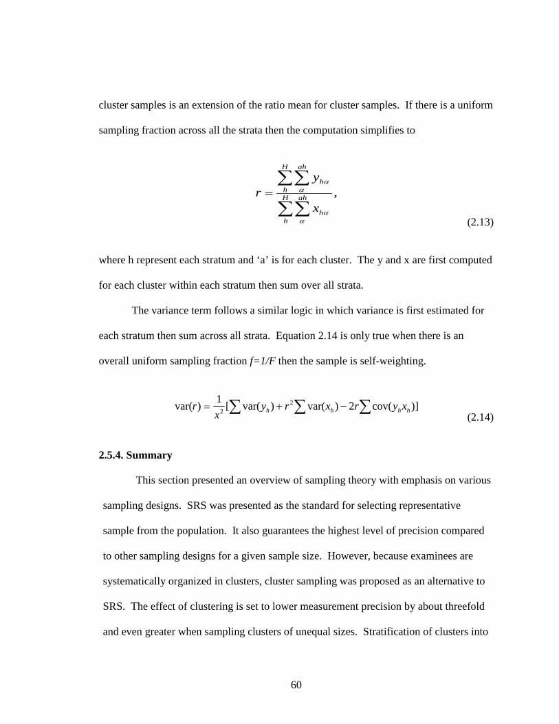
60
cluster samples is an extension of the ratio mean for cluster samples. If there is a uniform
sampling fraction across all the strata then the computation simplifies to
,∑∑
∑∑= H
h
ah
h
H
h
ah
h
x
yr
αα
αα
(2.13)
where h represent each stratum and ‘a’ is for each cluster. The y and x are first computed
for each cluster within each stratum then sum over all strata.
The variance term follows a similar logic in which variance is first estimated for
each stratum then sum across all strata. Equation 2.14 is only true when there is an
overall uniform sampling fraction f=1/F then the sample is self-weighting.
∑ ∑ ∑−+= ])cov(2)var()var([1)var( 2
2 hhhh xyrxryx
r (2.14)
2.5.4. Summary
This section presented an overview of sampling theory with emphasis on various
sampling designs. SRS was presented as the standard for selecting representative
sample from the population. It also guarantees the highest level of precision compared
to other sampling designs for a given sample size. However, because examinees are
systematically organized in clusters, cluster sampling was proposed as an alternative to
SRS. The effect of clustering is set to lower measurement precision by about threefold
and even greater when sampling clusters of unequal sizes. Stratification of clusters into

61
homogenous strata using the ‘right variables’ has been shown to significantly improve
measurement precision.
In relation to the overall research objective to create equivalent groups for
equating the following conclusions are deduced from the sampling literature to justify
the methodology adopted. First, sample selection and variance estimation can be viewed
as two separate processes. Stratified cluster sample selection mechanism will be used to
build the equating groups. To estimate the precision of the equating function a
nonparametric bootstrap technique will be used. The justification for not using the
variance estimation shown in equation 2.14 is that the equating function is estimated for
the entire sample as a unit as oppose to each cluster within a stratum separately. Two
main reasons why sampling error and equating precision are not estimated for individual
strata are: first, it will lead to bias equating caused by restriction of range in the equating
variable since strata are based on AP score attribute from previous years. And second,
estimating the equating function on individual strata might result to small sample
equating. This will produce disproportional error variances across strata.
This section provided theoretical and research evidence to support the use of
school means and school size as ‘right’ classification variables. Hansen et al. (1953)
suggested that stratifying on a measure of the outcome variable will lead to the greatest
reduction in variance. Kish recommended that an effective technique to adjust for
sample size and its associated variance when dealing with unequal clusters is to stratify
on cluster size. Thus the sample frame has been divided into a 5x5 stratification grid
based on these two variables.

62
A final deduction is that stratification or matching on a vector of relevant
covariates will ultimately accomplish the same goal as stratifying on the propensity
score. Rosenbaum and Rubin (1983) illustrated that the major difficulty with
stratification on a vector of p covariate is that even with binary covariates the number of
matches increase by a factor of 2p. In the present design were each stratification variable
has five levels the result is a stratification grid made up of 25 strata.
63
CHAPTER III
METHODOLOGY
Chapter III summarizes the design of an equating study that uses large-scale,
operational examinee test data from three successive years for two College Board
Advanced Placement ® (AP®) examination titles: AP Chemistry and AP Spanish
Language. The overall purpose of this study is to investigate the precision and accuracy
of equating mixed-format test based on a random stratified cluster group (RSCG) data
collection design.
This chapter is divided into 6 main sections. Section 3.1 presents summary
description of the study design methodology. Section 3.2 describes and discusses the
rationales used for selecting the operational AP datasets considered to evaluate the
research hypotheses. Data preparations applied on the master datasets to create
operational datasets are also discussed in this section. In Section 3.3, detailed procedures
applied to the operational datasets to create experimental test forms for equating in a
hypothetical situation are explained. Section 3.4 presents a review of the observed-score
equating procedures used in this research. Section 3.5 presents statistical evaluation
criteria used to summarize equated scores from the various designs and equating
procedures. This section also discusses the various rationales used to establish the
hypothetical equating criteria relationship for the various finite populations. Finally
section 3.6 describes the general procedures and tools adopted to carry out the re-

64
sampling study. The research questions from Chapter I are repeated here for convenient
reference since they help guide the research design:
1. How efficient is a sampling grid stratification design based on previous year
average AP school performance and school size to predict stratified random
clusters of school for equating two alternate mixed-format test forms
administered during a subsequent year?
a. Are there differences between Model 1 and Model 2 in terms of:
i. Conditional equating precision measured by sampling variability of
equated scores?
ii. Conditional equating Bias?
iii. Overall equating precision and accuracy?
b. What are the minimum sample requirements for each model to ensure
acceptable levels of equating precision and accuracy?
2. How does the random stratified cluster group (RSCG) design model compare
to Random cluster NEAT design with MC only common items? To simple
random cluster design?
a. Are there significant differences as measured by equating bias?
b. What is the design effect between the RSCG and NEAT design, and RG
and RSCG design?
c. What is the impact of form difficulty combination of mixed-format test on
equating accuracy

65
3. How much precision and accuracy is gained when the stratification framework
is based on more than one year of school aggregated data to predict current
year equivalent cluster of schools?
a. What is the amount of increase in accuracy of predicting equivalent school
strata?
b. What is the amount of increase in overall equating error between the two
models?
c. Are these effects consistent across the different AP subjects?
3.1. Study Methodology
3.1.1. Overview
The goal of this research is to evaluate the accuracy and precision to estimate an
equating function using a random stratified cluster group (RSCG) data collection design.
The main configuration of the stratified clusters is based on two stratifying variables—
average school performance and school size from previous year(s) test data. A sample of
examinees from these randomly stratified schools will then be used to estimate the
equating function for two or more alternate mixed-format test forms administered in the
subsequent year. The main hypothesis is that stratification on average AP school
performance from previous years will ensure that randomly equivalent samples of
schools are selected to estimate the equating function along the entire score scale.
The effect of clustering has been shown to increase overall sampling variance as
within school variance is generally smaller than between school variance. Students from
the same school are exposed to joint influences and as a result tend to be more similar. In

66
order to improve the accuracy of sample estimates when sampling from clusters,
stratifying on relevant covariates will generally increase within cluster homogeneity
which in turn will increase the overall sample heterogeneity. Studies by Henson,
Hurwitz, and Madow (1953) and Cochran (1963) confirm that rate of homogeneity within
clusters tends to decrease for larger clusters (i.e., large clusters tend to be more
heterogeneous). Thus by applying a probability proportionate to size selection method
on average AP school performance and school size, the proposed framework has the
necessary parameters in place to sample equivalent clusters of schools that are
representative of the population.
Two experimental sampling models using probability proportionate to size (PPS)
selection method were used to investigate the efficacy of equating mixed-format test
under the RSCG designs. Illustrations of Models 1 and 2 are shown in Figure 3.1. In the
first model (Model 1), a small proportionate sample will be drawn from the population
stratified frame. Then the estimated population equating relationship (EPEF) between the
forms will be estimated using the sample and the larger frame. The rationale of this
design is to limit the exposure of items on the form administered to the smaller sample so
it could be reused in the future.
In the second model (Model 2), two random samples of approximately equal sizes
will be drawn from the population stratified frame. These two random samples will be
used to estimate the EPEF of alternate mixed-format forms. The rationale is that the two
samples are equal and representative of the population. This model is practical for

67
situations in which scores have to be reported before all test data is available or to address
test malpractice at certain centers.
Figure 3.1. Sampling Plan for Model 1 and Model 2
3.2. Operational Dataset Transformation
Datasets used for this dissertation were from the College Board’s Advanced
Placement® (AP®) program. The AP® program consists of 30 exams covering about 22
content areas administered in high schools across USA and overseas. The goal of AP ®
is to provide high school students with the opportunity to take and earn credits in college
level courses. The AP exams test students’ ability to perform at a college level.
Currently all AP ® exams are of mixed-format with majority having the conventional
MC and CR item formats. The CR sections on these exams range from short responses to
open essay questions. A few of the AP exams however include other combinations of

68
item types. Examples of subjects with item types other than CR are AP Studio Arts
which has a portfolio assessment and AP World Languages which in addition to MC and
CR sections also has a speaking section.
In May 2010, 1.8 million students representing more than 17,000 schools around
the world, both public and nonpublic, took 3.2 million College Board AP ®
examinations worldwide. AP final grades are reported using a five point scale (1-5).
The American Council on Education recommends that colleges and universities grant
credit and/or placement into higher-level courses to entrants with AP Exam grade of 3 or
higher.
Two AP tests, AP Chemistry and AP Spanish Language, were selected for this
research study. Examinee level data from these tests were aggregated and manipulated
to create fixed “experimental” conditions which allowed the researcher to address the
research questions posed earlier. It should be noted that the examinee performance data
generated for this study do not reflect actual AP scores or score distributions reported by
College Board. Therefore, no attempts should be made to compare the aggregate results
presented in this study with published College Board AP data.
Four main factors guided the choice of the two College Board AP test titles
chosen for this research: (a) both examinations were mixed-format; (b) neither exam had
undergone major content or format changes over the three-year period investigated; (c)
the two test titles presented a representative range of covariance (correlational) patterns
between the MC and CR item-specific scales, with Chemistry tending to have higher and

69
more stable covariance patterns than Spanish; and (d) both had large sample sizes per
test administration.
The criterion that the subject examinations be mixed format should be obvious,
since the purpose of this dissertation is to investigate the potential value of a new data-
collection (i.e., sampling) design for equating mixed-format test. Summary descriptions
of the various AP tests used were obtained from the College Board website on AP
Exams. AP Chemistry exam is mixed-format with MC and CR item types. The exam is
divided into two sections. Section one is made up of 75 MC items that cover a broad
range of topics. Section two consists of six CR questions: three multipart quantitative
questions, one question on writing balanced chemical equations and answering a short
question for three different sets of reactants, and two multipart questions that are
essentially non quantitative. Both sections are also equally weighted towards the final
composite score.
AP Spanish Language exam is also of mixed-format, with a broader range of CR
item formats. In addition to traditional written CR items, AP Spanish also includes
speaking and listening prompts. AP Spanish evaluates students’ levels of performance in
the use of the language, both in understanding written and spoken Spanish. It measures
the students’ ability to write and speak with ease in correct and idiomatic Spanish in
interpersonal and presentational modes. The exam is divided into two main sections.
Section one is made up of 70 MC items with focus on two skills: reading and listening.
Section two focuses on writing and speaking: the writing skill section is made up of two
written prompts and the speaking section has 7 speaking prompts ranging from

70
conversational speaking to oral presentation. The relative weight of each skill in
calculating the final AP score is as follows: listening, 20%; reading, 30%; writing, 30%;
and speaking, 20%.
The second factor considered for selection of the three AP tests was that the actual
exam format had not undergone any major changes during the three year period. This
was a very important consideration as it allowed the research design to treat form
differences across year as a random variable. This also allowed the researcher to justify
the use of test scores from previous years to design a sampling plan for the subsequent
year.
The third factor considered was that the tests selected were representative of the
range of differential covariance structures observed across all the different 22 AP content
areas. An attempt was made to select AP subjects that will cover the range of MC and
CR correlation reported in the literature. Two AP subjects (Chemistry and Spanish
Language) a science and an arts were selected for this dissertation. This will ensure a
representative sample of AP tests with mixed-format characteristics. A noticeable trend
from the literature is that the correlation between MC and CR in AP science tests is
highest and in most cases almost unity after correction for measurement error is allowed.
Whereas, the Arts and languages tend to show the lowest correlation coefficient between
MC and CR formats. The observed correlation coefficient (see Appendix A) from the
operational test scores confirms this pattern.
The fourth and final factor considered for selection was that the sample size for
each test was large enough to assure reasonable standard error estimates in a replicated

71
sampling design without replacement. Sample sizes and sampling error are inversely
related; a larger sampling frame is always desirable in a sampling study. The selected
tests are administered to more than 90,000 examinees each year. Another important
consideration was total number of high schools since unit of selection is based on a
cluster of examines from the same high school. The total number of high schools range
from 7236 (Chemistry 2010) to 6343 (Spanish Language 2009). Table A.1 and Table
A.2 in Appendix A show the complete descriptive summary for each test across three
years. The tables include complete descriptive s of the various AP test by item type,
school size, classical test univariate, and bivariate statistics.
3.2.1. Data Preparation
The MC section of the AP exams used in this study was formula scored. AP no
longer uses formula scoring in its MC section. With formula scoring, for a MC item with
four response options, selecting an incorrect response option amounts to a fractional
penalty scoring function (sometimes referred to as the “K-factor” or “guessing penalty”),
where K is deducted from the total score for each incorrectly answered item. Omitted
items, in contrast, are replaced with a score of zero. The examinees are therefore reward
for omitting rather than incorrectly guessing items about which they are unsure as to the
correct answer. The K-factor for AP Chemistry was -0.25 and for AP Spanish it was—
0.332. The effect is an incomplete examinee response matrix as a result of examinees
skipping items to avoid the penalty. For all analyses in this research formula scoring
2 In 2012, The College Board AP Program implemented an empirically informed policy decision to abandon the “guessing penalty” and to move to rights-only scoring—including making corresponding changes in the instructions to the examinees.

72
protocol were maintained. The rationale was to avoid introducing new sources of bias by
implementing a missing data imputation algorithm. In the final dataset, examinees with a
negative total score were assigned a score of zero.
Another modification made to the master datasets was to remove schools with less
than 15 examinees from the equating frame. This was done to overcome the effect of
extreme school means for smaller schools that may have skewed the sampling results
within strata. Finally, schools were matched across all three years (2008, 2009 and 2010)
and only schools with more than 15 examinees in all three years were used in the
sampling frame. The total number of schools and examinees maintained in the
experimental finite population frame from operational datasets are shown in Table 3.1
and Table 3.2. The tables also show the corresponding sampling frame for each AP
subject.
Table 3.1. Population and Sampling Frame for AP Chemistry
Item
AP Chemistry
Year 2008 2009 2010 Population N (High Schools) 2,353 2,440 2,717
N (Students) 66,624 70,198 79,523
Frame n (High Schools) 1,403 (60) 1,403 (58) 1,403 (52)
n (Students) 46,868 (70) 48,311 (69) 50,115 (63) Note. ( ) indicates percentage from population
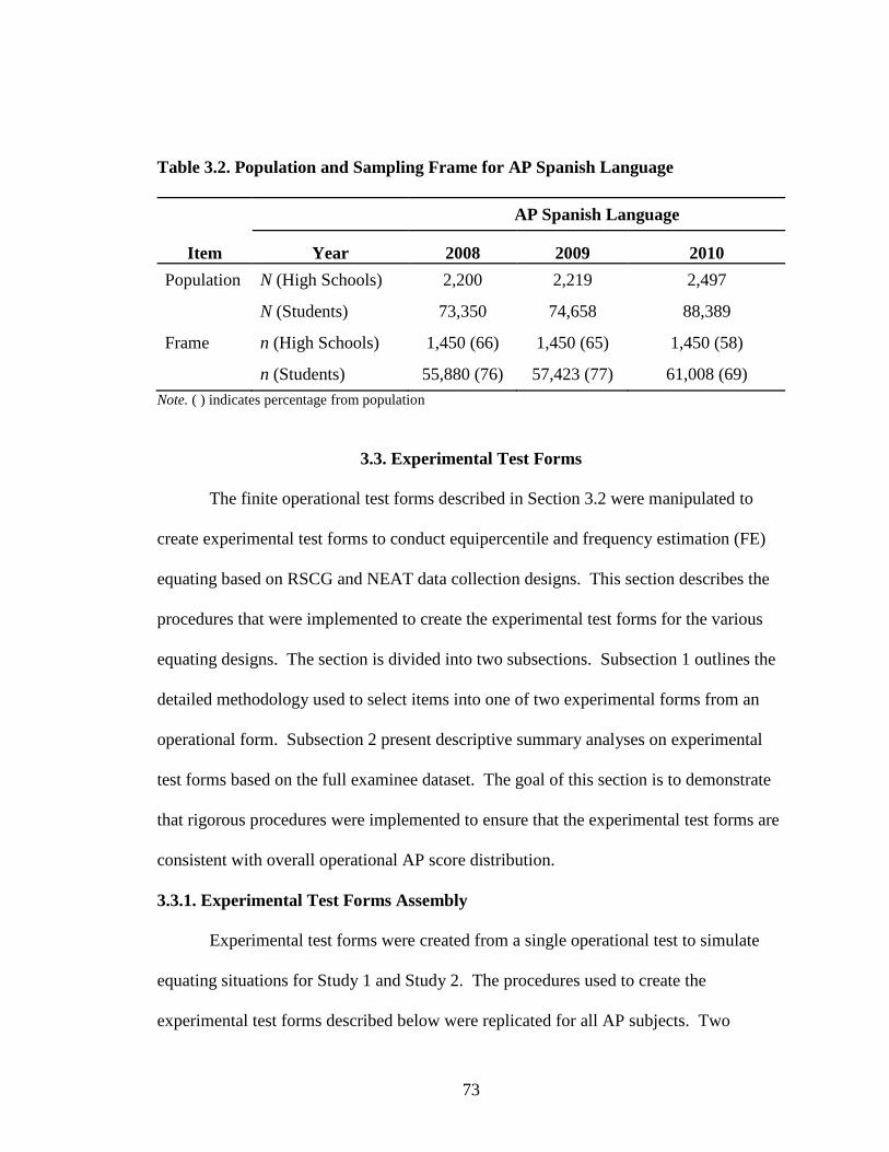
73
Table 3.2. Population and Sampling Frame for AP Spanish Language
Item
AP Spanish Language
Year 2008 2009 2010 Population N (High Schools) 2,200 2,219 2,497
N (Students) 73,350 74,658 88,389
Frame n (High Schools) 1,450 (66) 1,450 (65) 1,450 (58)
n (Students) 55,880 (76) 57,423 (77) 61,008 (69) Note. ( ) indicates percentage from population
3.3. Experimental Test Forms
The finite operational test forms described in Section 3.2 were manipulated to
create experimental test forms to conduct equipercentile and frequency estimation (FE)
equating based on RSCG and NEAT data collection designs. This section describes the
procedures that were implemented to create the experimental test forms for the various
equating designs. The section is divided into two subsections. Subsection 1 outlines the
detailed methodology used to select items into one of two experimental forms from an
operational form. Subsection 2 present descriptive summary analyses on experimental
test forms based on the full examinee dataset. The goal of this section is to demonstrate
that rigorous procedures were implemented to ensure that the experimental test forms are
consistent with overall operational AP score distribution.
3.3.1. Experimental Test Forms Assembly
Experimental test forms were created from a single operational test to simulate
equating situations for Study 1 and Study 2. The procedures used to create the
experimental test forms described below were replicated for all AP subjects. Two

74
separate pairs of experimental test forms were created from the 2009 and 2010
operational tests in Chemistry and Spanish.
Figure 3.2 shows the general framework used to create experimental forms. This
figure uses AP Chemistry 2009 operational test to illustrate the steps described below on
how each operational test form was manipulated to create two alternate mixed-format
experimental test forms. Similar procedures were replicated for 2010 and for AP Spanish
Language by modifying the appropriate number of items for each test year and subject.
Step 1 The joint examinee response matrix for the mixed-format test was
separated into two subgroups based on item format—CR (N x CR Items)
and MC (N x MC Items).
Step 2a The CR item response matrix was divided into two parallel groups
matched to satisfy a pre-defined standardized mean difficulty based on
observed scores. When possible both sets of CR forms were matched on
item specification type.
Step 2b For the MC items, first a set of anchor items (24 for AP Chemistry 2009)
were extracted from the 74 MC item response matrix. Then delta statistics
were used to build two alternate test forms constrained to satisfy a
predetermined standardized mean difference difficulty.
Step 3a RG For the RSCG design, the 24 anchor items were added to each parallel CR
and MC half and treated as non-common items. For example,
experimental test form 1 comprised of the sections as shown in Figure 3.3.

75
Figure 3.2. Experimental Test Form Schematic
Figure 3.3. Equating Design for RSCG Experimental Forms

76
Step3b For the NEAT design, the experimental forms were created as in step 3a
above but this time the MC_CI items were treated as traditional anchor.
That is the data collection design was setup to reflect a truly NEAT
condition with MC only anchor items. Figure 3.4 outlines the basic
structure of the data collection designs with experimental test forms for
the NEAT design.
Figure 3.4. Equating Design for NEAT Experimental Forms
The rationale for using the same item design template to create the RSCG and
NEAT experimental test form is to allow direct comparison of results between the two
data collection designs. Also, anchor items made up about 50% of total MC items on
each form. The reason is to ensure that any differences between designs are not
confounded by low reliability of anchor items. Thus results will indicate a conservative
estimate of actual expected differences.
3.3.2. Descriptive Summaries of Experimental Test Forms
Based on the framework presented, a total of 16 experimental test forms
constituting 8 pair of alternate forms were created from 4 operational AP exams in 2
subjects—Chemistry and Spanish Language. Table 3.3 shows the complete 2 x 2 x 2

77
experimental test forms design created for the entire study. Two conditional sets of
experimental test forms were created from each operational test using the 2009 and 2010
datasets.
Table 3.3. Standardized Effect Size for Alternate Experimental Mixed-Format Pairs
Form Condition
Chemistry Spanish
2009 2010 2009 2010 EE_HH .15* .21 .24 .19
EH_HE .03 .06 .15 .11 * Effect Size (ES) =
)2/)(( 21
21
sdsd +− χχ
The first condition labeled EE_HH represent a mixed-format experimental test
pair in which relatively easy MC and CR sections were combined to create one form.
The second alternate form was a combination of on average, more difficult CR and MC
items. Whereas, for the EH_HE pair condition, one form was a combination of on
average easier MC items but harder CR items. The alternate form was made up of harder
MC items and easier CR items. Measure of form difficulty was based on observed
proportion correct. The values in the table represent the average observed standardized
effect size differences (ES) between alternate forms in each condition. Complete
descriptive summaries on each pair of experimental test forms by AP subject are
presented in Tables 3.4 through 3.7. For all equating scenarios, experimental test form
labeled Exp_F2 was set as the base form. Scores from the alternate form Exp_F1 were
equated onto the scale of the base form (Exp_F2).

78
Table 3.4. AP Chemistry 2009 Operational and Experimental Test Forms Statistics
COMP1 is the weighted total of CR weighted scores and MC weighted scores. 2 The ( ) shows the Pearson correlation coefficient corrected for attenuation.
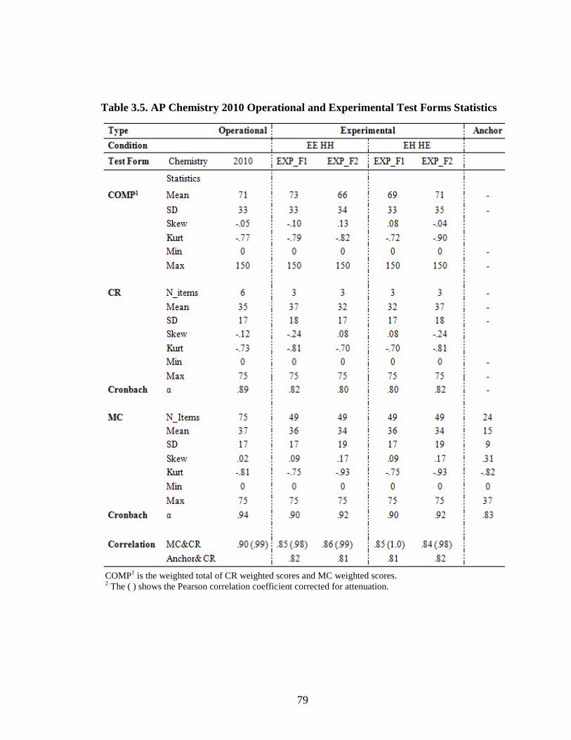
79
Table 3.5. AP Chemistry 2010 Operational and Experimental Test Forms Statistics
COMP1 is the weighted total of CR weighted scores and MC weighted scores. 2 The ( ) shows the Pearson correlation coefficient corrected for attenuation.

80
Table 3.6. AP Spanish 2009 Operational and Experimental Test Forms Statistics
COMP1 is the weighted total of CR weighted scores and MC weighted scores. 2 The ( ) shows the Pearson correlation coefficient corrected for attenuation.

81
Table 3.7. AP Spanish 2010 Operational and Experimental Test Forms Statistics
1COMP is the weighted total of CR weighted scores and MC weighted scores. 2 The ( ) shows the Pearson correlation coefficient corrected for attenuation.
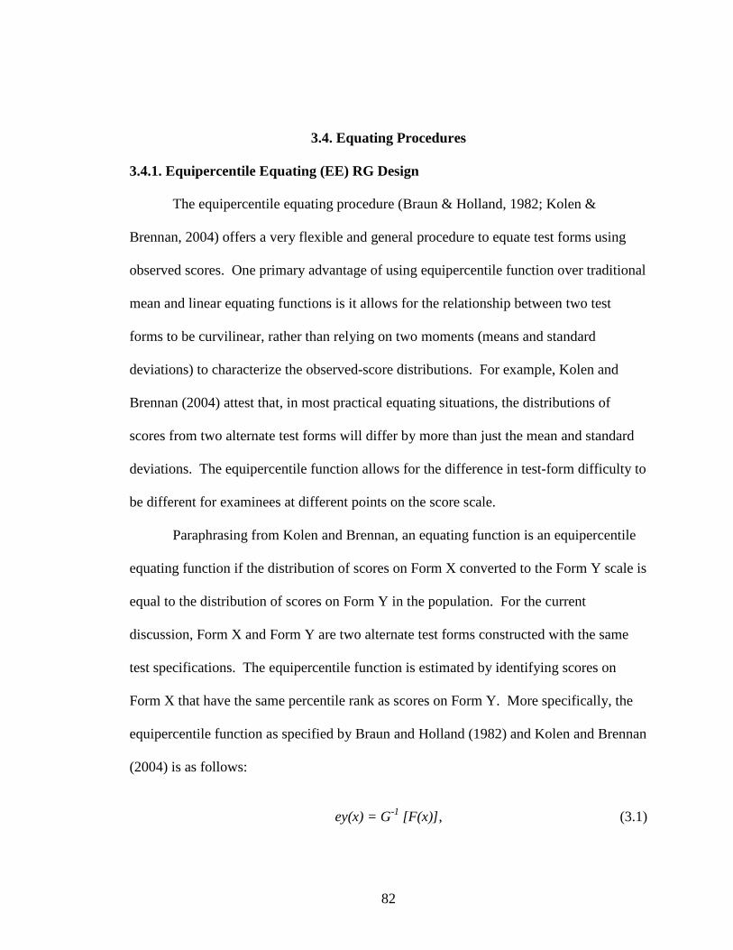
82
3.4. Equating Procedures
3.4.1. Equipercentile Equating (EE) RG Design
The equipercentile equating procedure (Braun & Holland, 1982; Kolen &
Brennan, 2004) offers a very flexible and general procedure to equate test forms using
observed scores. One primary advantage of using equipercentile function over traditional
mean and linear equating functions is it allows for the relationship between two test
forms to be curvilinear, rather than relying on two moments (means and standard
deviations) to characterize the observed-score distributions. For example, Kolen and
Brennan (2004) attest that, in most practical equating situations, the distributions of
scores from two alternate test forms will differ by more than just the mean and standard
deviations. The equipercentile function allows for the difference in test-form difficulty to
be different for examinees at different points on the score scale.
Paraphrasing from Kolen and Brennan, an equating function is an equipercentile
equating function if the distribution of scores on Form X converted to the Form Y scale is
equal to the distribution of scores on Form Y in the population. For the current
discussion, Form X and Form Y are two alternate test forms constructed with the same
test specifications. The equipercentile function is estimated by identifying scores on
Form X that have the same percentile rank as scores on Form Y. More specifically, the
equipercentile function as specified by Braun and Holland (1982) and Kolen and Brennan
(2004) is as follows:
ey(x) = G-1 [F(x)], (3.1)

83
where ey(x) is the equated Form X score on Form Y scale, G-1 is the inverse of the
cumulative distribution function of Form Y and F(x) is the cumulative distribution
function of Form X. Kolen and Brennan (2004) also expressed the symmetry property of
the equipercentile function in a similar manner:
ex(y) = F-1 [G(y)], (3.2)
where equation 3.2 is the symmetric function of equation 3.1 for equating Form Y on
Form X scale.
The estimation process of equipercentile function depends on first obtaining the
percentile rank for each score along the entire score scale. When the score scale
distribution is continuous, and there are enough examinees at each score point then
percentile ranks are directly computed from the observed score distribution. The reality
is that the score scale in most educational and psychological test are discrete. Holland
and Thayer (1989) outlined a statistical method using percentiles and percentile ranks
with continuization of the discrete score distributions, using the lower- and upper-real
limits. Their technique involves merely adding a uniform random variable over the range
of -0.5 to +0.5 to each discrete score point to create a continuous distribution.
To find a Form X score (xi) equipercentile equivalent for a Form Y percentile
rank the inverse to the percentile rank function is calculated as shown in equation 3.3
(Kolen & Brennan, 2004, p. 45):
),5.(
)()1()(100/
][ ***
**1 ++
−+−
=−L
LL
L xxFxF
xFppp
(3.3)

84
where *Lx represent the continuation of score xi and 0 < p* ≤ 100.
A potential drawback when percentile and percentile ranks are used to estimate
the equipercentile function is that the equating function is not sufficiently precise. This is
because the distribution of the equipercentile relationship appears irregular. Smoothing
methods have been developed to smooth the score distribution while maintaining the
central moments of the distribution. Kolen and Brennan (2004) described two broad
types of smoothing procedures: presmoothing and postsmoothing.
With presmoothing the raw score distribution are smoothed before equating using
either a polynomial log-linear method developed by Darroch and Ratcliff (1972),
Haberman (1972a, 1972b), Rosenbaum and Thayer (1987), or a strong true-score method
developed by Lord (1965). Postsmoothing on the other hand, is performed on the
equated equipercentile transformed scores. This is usually accomplished by fitting a
curve to the equipercentile scores using the cubic spline method developed by Reinsch
(1967). In-depth presentations of various smoothing methods have been presented by
Kolen and Brennan (2004).
Smoothing methods are designed to produce smooth functions which contain less random error than that for unsmoothed equipercentile equating. However, smoothing methods can introduce systematic error. The intent in using a smoothing method is for the increase in systematic error to be more than offset by the decrease in random error. (Kolen & Brennan, 2004, p. 70) There are no definite standard procedures in selecting between pre-smoothing
strategies and post-smoothing strategies, nor is there much research about technical
properties of the various statistical smoothers typically used in equating (e.g. choices of

85
bandwidth, kernel functions and the smoothing functions, themselves). Kolen and
Brennan recommend that the decision and choice about pre- versus post-smoothing
should be empirically evaluated. It is also clear that more research involving pre- and
post-smoothing methods for equating applications should be conducted in the future. For
the current research study a decision was made to evaluate only the unsmoothed
equipercentile conversion. Given that reasonably large samples were used in equating,
the expected difference between the smooth conversions and raw conversion are
negligible.
3.4.2. Frequency Estimation (FE) NEAT Design
In a NEAT design, examinees from potentially two different populations are
administered two different forms of a test. Form X is administered to a sample of
examinees from Population 1 and Form Y is administered to a sample of examinees from
Population 2. Both forms have some items in common generally referred to as anchor
items. The challenge in equating using the NEAT design is that examinees from
Population 1 where not administered Form Y and examinees from Population 2 where
not administered Form X.
The FE for NEAT design is an extension of the equipercentile method illustrated
above for the RG design. In the NEAT design, the score distributions of the anchor items
are used to express the synthetic distribution for Population 1 on Form Y and Population
2 on Form X. Kolen and Brennan (2004) expressed that these Form X and Form Y
distribution of the synthetic populations are a weighted combination of the distribution
for each population.

86
)()()( 2211 xfwxfwxf s += (3.4)
and
),()()( 2211 ygwygwyg s += (3.5)
where the subscript s refers to the synthetic population, 1 refers to the population
administered Form X and 2 the population administered Form Y, f and g are the
cumulative distribution of Form X and Y respectively and w1 and w2 (w1 + w2 = 1) are
used to weight the populations.
From equations 3.4 and 3.5, f2(x) and g1(y) are not directly observed from data
collected using the NEAT design. Estimating these distributions from available data
requires making the statistical assumption that for both Form X and Form Y, the
conditional distribution of total score given each anchor score (v), is the same in both
populations. Equation 3.6, adopted from Kolen and Brennan (2004), expresses this
assumption using quantities for which direct estimates are available from data collected.
f2(x,v) = f1(x/v) h2 (v) and g1(y,v) = g2 (y/v) h1 (v) (3.6)
In Population 2, f2(x,v) represent the joint distribution of total scores and anchor item
scores, h2 represent the distribution of scores on the common items. Similar
interpretation is made for Population 1.
Thus, substituting equation 3.6 into equations 3.4 and 3.5, respectively, provides
the following expressions for estimating the synthetic distribution in both populations:

87
)()|()()( 21211 vhvxfwxfwxf
vs ∑+=
(3.7)
and
),()()|()( 22121 ygwvhvygwyg
vs += ∑
(3.8)
where f1(x) is the probability of earning a score of x in population 1, f1(x|v) is the
conditional probability of a score of x in Form X for examinees with a particular score on
the anchor item in population 1 and h2(v) is the probability of having an anchor score v
in Population 2. The weighted products of these two probabilities are sum over all
anchor scores (v). The cumulative distribution gs(y) is similarly derived.
Kolen and Brennan then demonstrated using numerical examples that the FE
function for the NEAT design can be derived from the synthetic distributions from
equation 3.9, which is analogous to the equipercentile relationship for the RG design
presented in equation 3.2.
eys (x) = Q-1 [Ps (x)] (3.9)
The unsmoothed FE equating function was analyzed for all conditions in this research
study. Under the NEAT design the weights were fixed at one for the synthetic population
for the group taking the old test form.
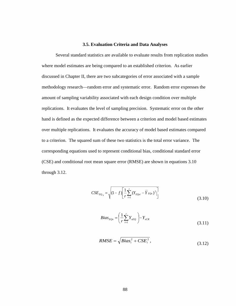
88
3.5. Evaluation Criteria and Data Analyses
Several standard statistics are available to evaluate results from replication studies
where model estimates are being compared to an established criterion. As earlier
discussed in Chapter II, there are two subcategories of error associated with a sample
methodology research—random error and systematic error. Random error expresses the
amount of sampling variability associated with each design condition over multiple
replications. It evaluates the level of sampling precision. Systematic error on the other
hand is defined as the expected difference between a criterion and model based estimates
over multiple replications. It evaluates the accuracy of model based estimates compared
to a criterion. The squared sum of these two statistics is the total error variance. The
corresponding equations used to represent conditional bias, conditional standard error
(CSE) and conditional root mean square error (RMSE) are shown in equations 3.10
through 3.12.
−−= ∑
=
r
iEQxEQxixEQ YY
rfCSE
1
2)(1)1( (3.10)
xCR
r
ixEQEQx YY
rBias −
= ∑
=1
1
(3.11)
,22ii CSEBiasRMSE += (3.12)
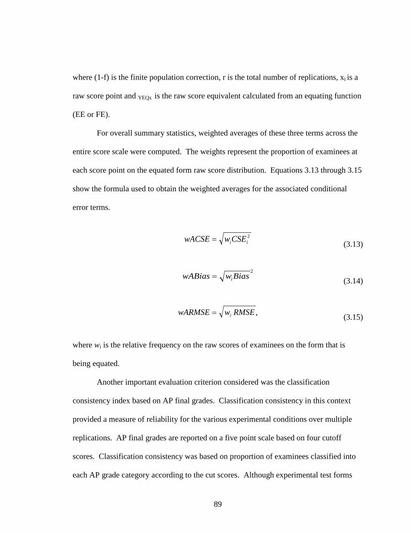
89
where (1-f) is the finite population correction, r is the total number of replications, xi is a
raw score point and YEQx is the raw score equivalent calculated from an equating function
(EE or FE).
For overall summary statistics, weighted averages of these three terms across the
entire score scale were computed. The weights represent the proportion of examinees at
each score point on the equated form raw score distribution. Equations 3.13 through 3.15
show the formula used to obtain the weighted averages for the associated conditional
error terms.
2iiCSEwwACSE = (3.13)
2
BiaswwABias i= (3.14)
,RMSEwwARMSE i= (3.15)
where wi is the relative frequency on the raw scores of examinees on the form that is
being equated.
Another important evaluation criterion considered was the classification
consistency index based on AP final grades. Classification consistency in this context
provided a measure of reliability for the various experimental conditions over multiple
replications. AP final grades are reported on a five point scale based on four cutoff
scores. Classification consistency was based on proportion of examinees classified into
each AP grade category according to the cut scores. Although experimental test forms
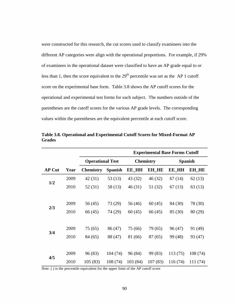
90
were constructed for this research, the cut scores used to classify examinees into the
different AP categories were align with the operational proportions. For example, if 29%
of examinees in the operational dataset were classified to have an AP grade equal to or
less than 1, then the score equivalent to the 29th percentile was set as the AP 1 cutoff
score on the experimental base form. Table 3.8 shows the AP cutoff scores for the
operational and experimental test forms for each subject. The numbers outside of the
parentheses are the cutoff scores for the various AP grade levels. The corresponding
values within the parentheses are the equivalent percentile at each cutoff score.
Table 3.8. Operational and Experimental Cutoff Scores for Mixed-Format AP Grades
Experimental Base Forms Cutoff
Operational Test Chemistry Spanish
AP Cut Year Chemistry Spanish EE_HH EH_HE EE_HH EH_HE
1/2 2009 42 (31) 53 (13) 43 (32) 46 (32) 67 (14) 62 (13)
2010 52 (31) 58 (13) 46 (31) 51 (32) 67 (13) 63 (13)
2/3 2009 56 (45) 73 (29) 56 (46) 60 (45) 84 (30) 78 (30)
2010 66 (45) 74 (29) 60 (45) 66 (45) 85 (30) 80 (29)
3/4 2009 75 (65) 86 (47) 75 (66) 79 (65) 96 (47) 91 (49)
2010 84 (65) 88 (47) 81 (66) 87 (65) 99 (48) 93 (47)
4/5 2009 96 (83) 104 (74) 96 (84) 99 (83) 113 (75) 108 (74)
2010 105 (83) 108 (74) 103 (84) 107 (83) 116 (74) 111 (74) Note. ( ) is the percentile equivalent for the upper limit of the AP cutoff score

91
The classification consistency indices were computed as the percentage of
instances that the same decision was reached based on result from the EPEF and the SG
criterion. This is the sum of proportions on the diagonal of a 5x5 contingency table of
model and criterion based proportion of examinees at each AP grade level.
5544332211 ppppppi ++++= (3.16)
The expected classification index is taken over 500 replications for each condition.
Higher indices of this proportion signify reliability of results over multiple replications.
Summary plots and tables comparing results based on these evaluation criteria are
presented in Chapter IV for each condition in the research design.
3.5.1. Equating Criterion
The hypothetical test design described above facilitated the establishment of
criteria for evaluating the various design conditions shown in Table 3.9. In reality, since
each alternate experimental Form 1 and Form 2 was created from a single test form (2009
or 2010), every examinee had observed scores on both forms. Therefore, Form 1 and
Form 2 can be directly equated using the single group design (SG). In hypothetical
research studies, the SG design has been shown to be the most efficient equating designs
in terms of accuracy and precision because examinees act as their own controls, with the
autocorrelation serving to reduce the equating error variance. It also has the advantage
that it requires the smallest sample size for any given level of precision compared to other
designs (Dorans et al., 2010; Kolen & Brennan, 2004).

92
Table 3.9. Equating Design Conditions
Condition Data Collection Test
Format Anchor Equating Method
RSCG1 Random Stratified Cluster Group MC+CR - EE2
RC1 Random Cluster MC+CR - EE
RCNEAT Random Cluster NEAT MC+CR MC FE3
1 Condition is replicated for model 1 and model 2. 2 Is the equipercentile estimation procedure for random groups design defined in Section 3.4 3 Frequency estimation procedure for NEAT design with anchor items define in Section 3.4
Livingston (1993) first proposed this approach to derive a plausible criterion
equating function for the total test under the observed equating framework.3 The direct
SG equipercentile conversion of raw scores between each pair of test forms serves as a
reliable estimate of the criterion for each hypothetical population and test design. With
an average of about 60,000 observations in each AP population frame, I am confident that
the criterion function is very stable and represent a reasonable measure of truth. These
SG equating functions based on all examinees are referred to hereafter as the reference
form equating (RFE) and will be established as the criterion to evaluate overall equating
error for the various models and equating designs.
3.5.2. Research Design
For each study and AP subject complete crossing of 2 pairs of mixed-format test
form conditions (Table 3.3), 5 equating design conditions (Table 3.9), and 4 sampling
rates (Table 3.10 and Table 3.11) produced a 40 (5x4x2) design resulting in a total of
20,000 equating after 500 replications.
3 This criterion does not reflect “truth” in any absolute sense. At best, it reflects higher or lower consistency in the results.
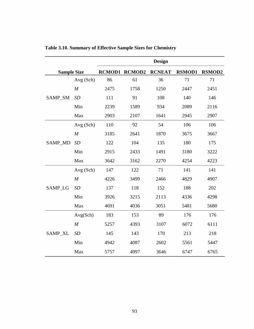
93
Table 3.10. Summary of Effective Sample Sizes for Chemistry
Sample Size
Design
RCMOD1 RCMOD2 RCNEAT RSMOD1 RSMOD2
SAMP_SM
Avg (Sch) 86 61 36 71 71
M 2475 1758 1250 2447 2451
SD 111 91 108 140 146
Min 2239 1589 934 2089 2116
Max 2903 2107 1641 2945 2907
SAMP_MD
Avg (Sch) 110 92 54 106 106
M 3185 2641 1870 3675 3667
SD 122 104 135 180 175
Min 2915 2433 1491 3180 3222
Max 3642 3162 2270 4254 4223
SAMP_LG
Avg (Sch) 147 122 71 141 141
M 4226 3499 2466 4829 4907
SD 137 118 152 188 202
Min 3926 3215 2113 4336 4298
Max 4691 4036 3051 5481 5680
SAMP_XL
Avg(Sch) 183 153 89 176 176
M 5257 4393 3107 6072 6111
SD 145 143 170 213 218
Min 4942 4087 2602 5561 5447
Max 5757 4997 3646 6747 6765
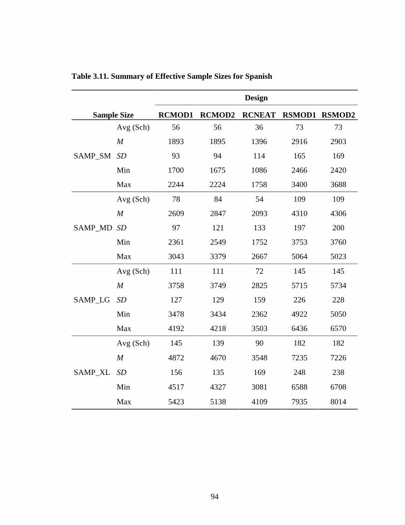
94
Table 3.11. Summary of Effective Sample Sizes for Spanish
Sample Size
Design
RCMOD1 RCMOD2 RCNEAT RSMOD1 RSMOD2
SAMP_SM
Avg (Sch) 56 56 36 73 73
M 1893 1895 1396 2916 2903
SD 93 94 114 165 169
Min 1700 1675 1086 2466 2420
Max 2244 2224 1758 3400 3688
SAMP_MD
Avg (Sch) 78 84 54 109 109
M 2609 2847 2093 4310 4306
SD 97 121 133 197 200
Min 2361 2549 1752 3753 3760
Max 3043 3379 2667 5064 5023
SAMP_LG
Avg (Sch) 111 111 72 145 145
M 3758 3749 2825 5715 5734
SD 127 129 159 226 228
Min 3478 3434 2362 4922 5050
Max 4192 4218 3503 6436 6570
SAMP_XL
Avg (Sch) 145 139 90 182 182
M 4872 4670 3548 7235 7226
SD 156 135 169 248 238
Min 4517 4327 3081 6588 6708
Max 5423 5138 4109 7935 8014

95
Sampling rates were preferred over exact sample sizes because when sampling
cluster of unequal sizes, sample size is a random variable. Two criteria influenced the
selection of effective sampling sizes. First, for RSMOD1 and RSMOD2, the exact
sampling rates were used to ensure that the same proportions of examinees were selected
from each population. Second, for the RCMOD1, RCMOD2 and RCNEAT designs,
variable sampling rates were used depending on the population frame. The justification
was to attempt to match the effective sample sizes selected in RSMOD1 and RSMOD2.
For each design it was imperative that the range of samples selected across the various
conditions (SAMP_SM, SAMP_MD, SAMP_LG and SAMP_XL) satisfies the minimum
sample size requirement of 1500 for equipercentile equating.
3.5.3. Data Analyses
Data analyses were organized in 3 main phases. For each model and AP subject
combination, sampling precision, equating accuracy, total error variance and
classification consistency for all 32 cells were analyzed accordingly by research
questions. In all, 48,000 equating functions were analyzed in this dissertation to generate
findings to address the following problems:
Problem 1: How efficient is a sampling grid stratification design based on previous year
average AP school performance and school size to predict random clusters of school for
equating two alternate mixed-format test forms administered during a subsequent year?
For Problem 1, a 2x2x4 research design shown in Figure 3.5 for each subject was
used to collect data using a bootstrap resampling framework. Observed score
equipercentile equating procedure was used to estimate the equating function for each

96
design condition. For each cell in the complete cross matrix 500 bootstrap replications
were conducted based on the experimental test forms created from the 2009 operational
sets in AP Chemistry and Spanish Language. Deviance statistics (Bias, CSE, and RMSE)
were computed and used to evaluate results between RSMOD1 and RSMOD2. Visual
inspection of plots and summary tables in conjunction with various evaluation criteria
averaged over the entire score range were used to inform the discussions and conclusions
in Chapter V. Tables of classification consistency for each model were also analyzed.
In addition both models were compared across the various sampling rate to
determine the minimum sample size requirements. Kolen and Brennan (2004)
recommended that appropriate sample sizes for equating are such that the SEE would be
less than .1 standard deviation unit on the raw score scale between z-score of -2 and +2.
Exam
SM MD LG XL SM MD LG XL
RSMOD1 √ √ √ √ √ √ √ √
RSMOD2 √ √ √ √ √ √ √ √
RSMOD1 √ √ √ √ √ √ √ √
RSMOD2 √ √ √ √ √ √ √ √
MTD n
Chem
istr
ySp
anis
h
ConditionTest Form Difficulty
EE_HH EH_HE
Figure 3.5. 2x2x4 Experimental Design for Research Question 1

97
Problem 2: How does the random stratified cluster groups (RSCG) design compare to a
NEAT design with MC only anchor items and a random cluster design?
For Problem 2 the design frame was expanded to a 5 data collection designs by 4
sampling rates by test form conditions for each subject (5x4x2) displayed in Figure 3.6.
Results and analyses were based on comparing equating results from all 5 equating
conditions. In addition to comparison plots of bias SEE, RMSE and classification
consistency, two new evaluation criteria were used to summarize findings.
First, a conservative criterion of the difference that matters or DTM (Dorans &
Feigenbaum, 1994) was used to evaluate the different equating relationships based on the
unsmoothed estimated equating functions. The DTM was defined as any difference that
is equal to or greater than 0.5 of the raw score. Based on this criterion, any difference
less than 0.5 is probably ignorable as it may not result in any practical difference in
examinees’ reported scores.
MTD n SM MD LG XL SM MD LG XL
RSMOD1 √ √ √ √ √ √ √ √RSMOD2 √ √ √ √ √ √ √ √RCNEAT √ √ √ √ √ √ √ √RCMOD1 √ √ √ √ √ √ √ √RCMOD2 √ √ √ √ √ √ √ √RSMOD1 √ √ √ √ √ √ √ √RSMOD2 √ √ √ √ √ √ √ √RCNEAT √ √ √ √ √ √ √ √RCMOD1 √ √ √ √ √ √ √ √RCMOD2 √ √ √ √ √ √ √ √
Che
mis
try
Span
ish
Exam ConditionTest Form Difficulty
EE_HH EH_HE
Figure 3.6. 5x4x2 Experimental Design for Research Question 2

98
The second criterion evaluated was the design effect. The design effect measures
the amount of error associated with RSCG sampling design over traditional random
sampling design. Design effect was defined as the ratio between the variance terms of
the RSCG and RC in each design condition.
Problem 3: How much precision and accuracy is gained when the stratification
framework is based on more than one year of school aggregated data to predict
subsequent year equivalent stratified cluster of schools.
A similar 2x2x4 research design present for Problem 1 (Figure 3.5) was used.
The major differences were that the experimental test form created from the 2010
operational data set was used in the equating. The sampling frame for the RSCG models
was based on an aggregate of the covariates from 2008 and 2009 data. Bootstrap
summary indices of accuracy, precision and classification consistency from the complete
design were compared using plots and tables. Difference between these indices and those
from 2009 were also analyzed to measure the amount of improvement by aggregating
covariates across more than one year. These estimates were also compared across the
two AP subjects to show whether these effects were consistent across the board.
3.6. Re-sampling Study
3.6.1. Data Collection Procedure
The following procedures were used to collect data for Study 1 and Study 2 from
already available examinee data. Two procedural variations have been outlined below.
The first set of procedures describes steps implemented for Study 1 and Study 2 under the
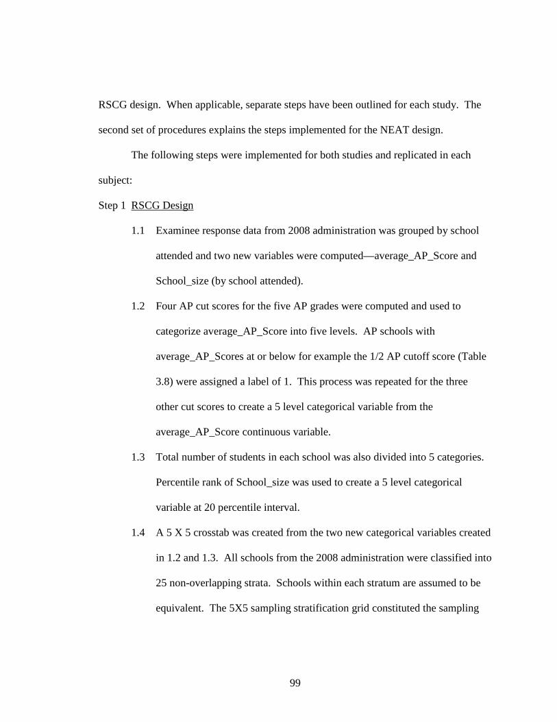
99
RSCG design. When applicable, separate steps have been outlined for each study. The
second set of procedures explains the steps implemented for the NEAT design.
The following steps were implemented for both studies and replicated in each
subject:
Step 1 RSCG Design
1.1 Examinee response data from 2008 administration was grouped by school
attended and two new variables were computed—average_AP_Score and
School_size (by school attended).
1.2 Four AP cut scores for the five AP grades were computed and used to
categorize average_AP_Score into five levels. AP schools with
average_AP_Scores at or below for example the 1/2 AP cutoff score (Table
3.8) were assigned a label of 1. This process was repeated for the three
other cut scores to create a 5 level categorical variable from the
average_AP_Score continuous variable.
1.3 Total number of students in each school was also divided into 5 categories.
Percentile rank of School_size was used to create a 5 level categorical
variable at 20 percentile interval.
1.4 A 5 X 5 crosstab was created from the two new categorical variables created
in 1.2 and 1.3. All schools from the 2008 administration were classified into
25 non-overlapping strata. Schools within each stratum are assumed to be
equivalent. The 5X5 sampling stratification grid constituted the sampling
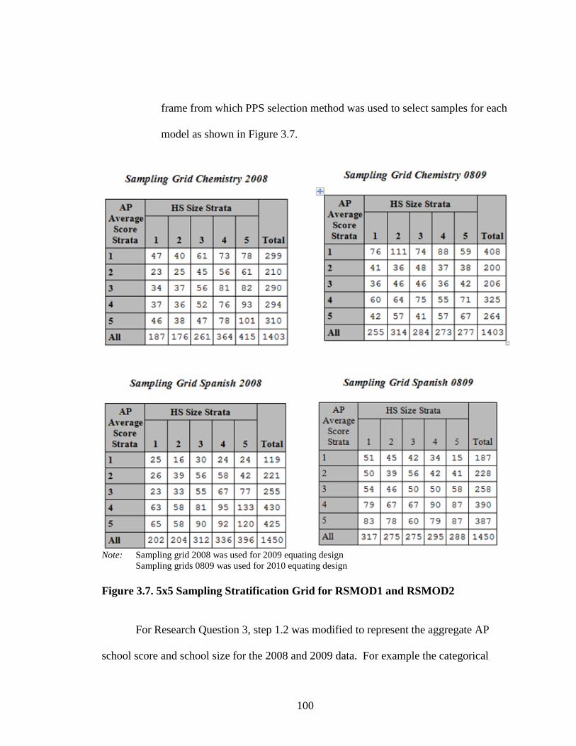
100
frame from which PPS selection method was used to select samples for each
model as shown in Figure 3.7.
Note: Sampling grid 2008 was used for 2009 equating design Sampling grids 0809 was used for 2010 equating design Figure 3.7. 5x5 Sampling Stratification Grid for RSMOD1 and RSMOD2
For Research Question 3, step 1.2 was modified to represent the aggregate AP
school score and school size for the 2008 and 2009 data. For example the categorical

101
variable of Average_AP_Score was the average AP classification between 2008 and 2009
classifications. The new categorical School_size variable was also derived in a similar
way. Figure 3.7 shows the sampling frames created for RSMOD1 and RSMOD2
conditions for each AP subject.
Step 2 NEAT Design
Once the RSCG sampling frames were established, the following modifications
were implemented to create two nonequivalent groups from the population and sampling
frame created in Step 1.
2.1 The total observed score based on the operational form was used as a
measure of ability to create two nonequivalent groups of schools. A SAS
conditional macro was written to split the population into two nonequivalent
groups. The average standardized effect size difference in ability between
the populations was set to range from 0.15 and 0.2.
2.2 The grouping variable created in 2.1 was used to split the sampling frame
created in step 1 into two nonequivalent groups. Table 3.12 and Table 3.13
show descriptive summary for NEAT groups sampling frame.
3.6.2. Replication Study
The entire replication study was conducted in SAS. SAS macros were written to
manipulate raw scores from operational test forms as discussed above. Realization of the
study for following conditions: 2 test difficulty conditions, 4 sample size conditions, 2
equating procedures, 3 data collection designs, 2 AP subjects and a pair of experimental
forms for two years was done as follows: First, using SAS proc survey select PPS
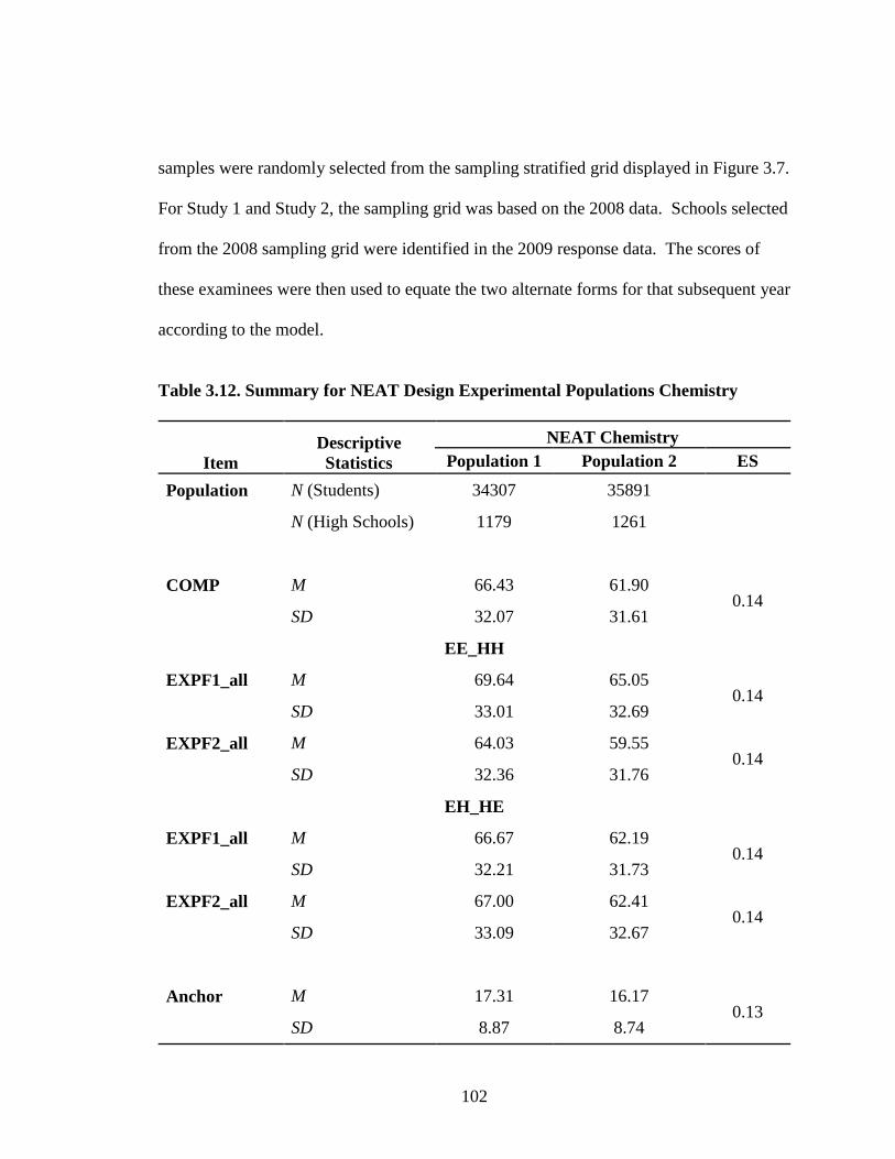
102
samples were randomly selected from the sampling stratified grid displayed in Figure 3.7.
For Study 1 and Study 2, the sampling grid was based on the 2008 data. Schools selected
from the 2008 sampling grid were identified in the 2009 response data. The scores of
these examinees were then used to equate the two alternate forms for that subsequent year
according to the model.
Table 3.12. Summary for NEAT Design Experimental Populations Chemistry
Item Descriptive Statistics
NEAT Chemistry Population 1 Population 2 ES
Population N (Students) 34307 35891
N (High Schools) 1179 1261
COMP M 66.43 61.90 0.14
SD 32.07 31.61
EE_HH
EXPF1_all M 69.64 65.05 0.14
SD 33.01 32.69
EXPF2_all M 64.03 59.55 0.14
SD 32.36 31.76
EH_HE
EXPF1_all M 66.67 62.19 0.14
SD 32.21 31.73
EXPF2_all M 67.00 62.41 0.14
SD 33.09 32.67
Anchor M 17.31 16.17 0.13
SD 8.87 8.74

103
Table 3.13. Summary for NEAT Design Experimental Populations Spanish
Item Descriptive Statistics
NEAT Spanish Population 1 Population 2 ES
Population N (Students) 36796 37862
N (High Schools) 1115 1104
COMP M 89.05 86.18 0.12
SD 24.44 24.84
EE_HH
EXPF1_all M 91.76 88.96 0.11
SD 25.35 25.85
EXPF2_all M 97.17 94.43 0.11
SD 24.12 24.75
EH_HE
EXPF1_all M 96.49 62.19 0.11
SD 25.21 25.86
EXPF2_all M 92.45 89.70 0.11
SD 24.55 25.08
Anchor M 21.76 21.04
0.1 SD 7.09 7.35
Second, for each combination of study conditions, observed-score equipercentile
(EE) and frequency estimation (FE) were used to equate each pair of alternate mixed-
format test forms. The computer program RAGE-RGEQUATE and CIPE (Kolen &
Brennan, 2004) was incorporated into SAS environment and used to perform EE and FE
equating procedures. Results from the Rage-RGEQUATE and CIPE programs were

104
validated using independent SAS macros written to perform EE and FE for RG and
NEAT designs.
Third, these procedures described above were replicated 500 times for each cell in
the design frame. The sampling distributions of equated scores at each score point over
500 replications were summarized using the evaluation criteria presented in Section 3.5.
Chapter IV presents results from these procedures for each research question.

105
CHAPTER IV
RESULTS
Chapter IV provides results for the three research questions presented in Chapter I
based on the methodology outlined in Chapter III. These results are presented using
summary tables and graphic illustrations computed from the evaluation criteria of CSE,
Bias, RMSE, wACSE, wABias wARMSE and classification consistency. This chapter is
organized into four main sections. Section 4.1 shows summary results of the criterion
equating based on a single group design and the equipercentile equating procedure.
Section 4.2 presents results for Research Question 1 based upon the differences between
RSMOD1 and RSMOD2. Section 4.3 presents results for Research Question 2 that
compares RSMOD1 and RSMOD2 with RCNEAT, RCMOD1 and RCMOD2. Section
4.4 presents results for Research Question 3 on the effect of equating accuracy when
covariates are aggregated over a period of two years.
4.1. Criterion Equating Analysis
Single group (SG) data collection design with equipercentile equating was used to
establish an empirical, baseline equating criteria. A total of eight criterion SG
equipercentile functions were estimated using all of the examinee data to approximate the
experimental population criterion equating functions for all eight pairs of test forms in the
2x2x2 design shown in Table 3.3. For all conditions, experimental form 2 (ExpF2) was
established as the base form and scores from form 1 (ExpF1) were equated onto the scale

106
of Form 2. Table 4.1 through Table 4.8 show the first four moments of ExpF1
equipercentile equated raw scores on the base form scale. The tables also include the
corresponding base form moments and the ExpF1 raw score moments.
Table 4.1. Equipercentile SG Equated Moments Chemistry EE_HH 2009
Moments Equ_F1_EE ExpF1_Raw ExpF2_Base
Mean 61.74 67.29 61.74
STD 32.13 32.93 32.13
Skew 0.17 -0.02 0.17
Kurt -0.76 -0.82 -0.76
Table 4.2. Equipercentile SG Equated Moments Chemistry EH_HE 2009
Moments Equ_F1_EH ExpF1_Raw ExpF2_Base
Mean 64.65 64.38 64.65
STD 32.95 32.05 32.95
Skew 0.04 0.10 0.04
Kurt -0.82 -0.77 -0.82
Table 4.3. Equipercentile SG Equated Moments Chemistry EE_HH 2010
Moments Equ_F1_EE ExpF1_Raw ExpF2_Base
Mean 66.33 73.03 66.33
STD 34.28 33.49 34.28
Skew 0.13 -0.10 0.13
Kurt -0.82 -0.79 -0.82
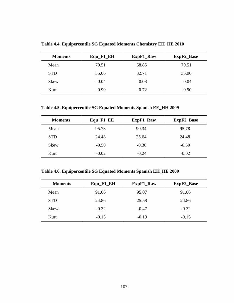
107
Table 4.4. Equipercentile SG Equated Moments Chemistry EH_HE 2010
Moments Equ_F1_EH ExpF1_Raw ExpF2_Base
Mean 70.51 68.85 70.51
STD 35.06 32.71 35.06
Skew -0.04 0.08 -0.04
Kurt -0.90 -0.72 -0.90
Table 4.5. Equipercentile SG Equated Moments Spanish EE_HH 2009
Moments Equ_F1_EE ExpF1_Raw ExpF2_Base
Mean 95.78 90.34 95.78
STD 24.48 25.64 24.48
Skew -0.50 -0.30 -0.50
Kurt -0.02 -0.24 -0.02
Table 4.6. Equipercentile SG Equated Moments Spanish EH_HE 2009
Moments Equ_F1_EH ExpF1_Raw ExpF2_Base
Mean 91.06 95.07 91.06
STD 24.86 25.58 24.86
Skew -0.32 -0.47 -0.32
Kurt -0.15 -0.19 -0.15

108
Table 4.7. Equipercentile SG Equated Moments Spanish EE_HH 2010
Moments Equ_F1_EE ExpF1_Raw ExpF2_Base
Mean 97.45 92.08 97.45
STD 26.16 25.72 26.16
Skew -0.62 -0.39 -0.62
Kurt 0.16 -0.19 0.16
Table 4.8. Equipercentile SG Equated Moments Spanish EH_HE 2010
Moments Equ_F1_EH ExpF1_Raw ExpF2_Base
Mean 93.17 96.36 93.17
STD 25.42 26.53 25.42
Skew -0.42 -0.58 -0.42
Kurt -0.10 0.02 -0.10
The equated summary of AP Chemistry test conditions shows that the SG
unsmoothed equipercentile function successfully preserved the first four moments on the
base form. Corresponding unsmoothed and smoothed conditional difference functions
with conditional 68% error bands for each criterion equating functions are displayed in
Figure 4.1 through Figure 4.8. The difference function is based on the difference between
the equipercentile function and an identity function at each raw score point. For example,
Figure 4.1 for condition EE_HH is made up of four plots with overlay difference
functions of unsmoothed and post-smooth equipercentile functions at four levels of
smoothing (.01, .05, .1, .2).

109
Eq
uat
ed E
xpF
1 M
inu
s E
xpF
1 R
aw
-9
-8
-7
-6
-5
-4
-3
-2
-1
0
1
Raw Score ExpF10 15 30 45 60 75 90 105 120 135 150
Eq
uat
ed E
xpF
1 M
inu
s E
xpF
1 R
aw
-9
-8
-7
-6
-5
-4
-3
-2
-1
0
1
Raw Score ExpF10 15 30 45 60 75 90 105 120 135 150
Eq
uat
ed E
xpF
1 M
inu
s E
xpF
1 R
aw
-9
-8
-7
-6
-5
-4
-3
-2
-1
0
1
Raw Score ExpF10 15 30 45 60 75 90 105 120 135 150
Eq
uat
ed E
xpF
1 M
inu
s E
xpF
1 R
aw
-9
-8
-7
-6
-5
-4
-3
-2
-1
0
1
Raw Score ExpF10 15 30 45 60 75 90 105 120 135 150
Equipercentile Raw-to Raw Score for Post-Smoothing, S = 0.01
SmoothedUnsmoothed+1 S.E.-1 S.E.
Equipercentile Raw-to Raw Score for Post-Smoothing, S = 0.05
SmoothedUnsmoothed+1 S.E.-1 S.E.
Equipercentile Raw-to Raw Score for Post-Smoothing, S = 0.1
SmoothedUnsmoothed+1 S.E.-1 S.E.
Equipercentile Raw-to Raw Score for Post-Smoothing, S = 0.2
SmoothedUnsmoothed+1 S.E.-1 S.E.
Figure 4.1. SG Criterion Equated Difference for Chemistry 2009 EE_HH (ES = .15)
Eq
uat
ed E
xpF
1 M
inu
s E
xpF
1 R
aw
-3
-2
-1
0
1
2
3
Raw Score ExpF1_EH0 15 30 45 60 75 90 105 120 135 150
Eq
uat
ed E
xpF
1 M
inu
s E
xpF
1 R
aw
-3
-2
-1
0
1
2
3
Raw Score ExpF1_EH0 15 30 45 60 75 90 105 120 135 150
Eq
uat
ed E
xpF
1 M
inu
s E
xpF
1 R
aw
-3
-2
-1
0
1
2
3
Raw Score ExpF1_EH0 15 30 45 60 75 90 105 120 135 150
Eq
uat
ed E
xpF
1 M
inu
s E
xpF
1 R
aw
-3
-2
-1
0
1
2
3
Raw Score ExpF1_EH0 15 30 45 60 75 90 105 120 135 150
Equipercentile Raw-to Raw Score for Post-Smoothing, S = 0.01
SmoothedUnsmoothed+1 S.E.-1 S.E.
Equipercentile Raw-to Raw Score for Post-Smoothing, S = 0.05
SmoothedUnsmoothed+1 S.E.-1 S.E.
Equipercentile Raw-to Raw Score for Post-Smoothing, S = 0.1
SmoothedUnsmoothed+1 S.E.-1 S.E.
Equipercentile Raw-to Raw Score for Post-Smoothing, S = 0.2
SmoothedUnsmoothed+1 S.E.-1 S.E.
Figure 4.2. SG Criterion Equated Difference for Chemistry 2009 EH_HE (ES = .03)

110
Eq
uat
ed E
xpF
1 M
inu
s E
xpF
1 R
aw
-10-9
-8-7
-6-5
-4-3-2
-10
1
Raw Score ExpF10 15 30 45 60 75 90 105 120 135 150
Eq
uat
ed E
xpF
1 M
inu
s E
xpF
1 R
aw
-10-9
-8-7
-6-5
-4-3-2
-10
1
Raw Score ExpF10 15 30 45 60 75 90 105 120 135 150
Eq
uat
ed E
xpF
1 M
inu
s E
xpF
1 R
aw
-10
-9-8
-7-6
-5-4
-3-2
-10
1
Raw Score ExpF10 15 30 45 60 75 90 105 120 135 150
Eq
uat
ed E
xpF
1 M
inu
s E
xpF
1 R
aw
-10
-9-8
-7-6
-5-4
-3-2
-10
1
Raw Score ExpF10 15 30 45 60 75 90 105 120 135 150
Equipercentile Raw-to Raw Score for Post-Smoothing, S = 0.01
SmoothedUnsmoothed+1 S.E.-1 S.E.
Equipercentile Raw-to Raw Score for Post-Smoothing, S = 0.05
SmoothedUnsmoothed+1 S.E.-1 S.E.
Equipercentile Raw-to Raw Score for Post-Smoothing, S = 0.1
SmoothedUnsmoothed+1 S.E.-1 S.E.
Equipercentile Raw-to Raw Score for Post-Smoothing, S = 0.2
SmoothedUnsmoothed+1 S.E.-1 S.E.
Figure 4.3. SG Criterion Equated Difference for Chemistry 2010 EE_HH (ES = .21)
Eq
uat
ed E
xpF
1 M
inu
s E
xpF
1 R
aw
-4
-3
-2
-1
0
1
2
3
4
5
6
Raw Score ExpF1_EH0 15 30 45 60 75 90 105 120 135 150
Eq
uat
ed E
xpF
1 M
inu
s E
xpF
1 R
aw
-4
-3
-2
-1
0
1
2
3
4
5
6
Raw Score ExpF1_EH0 15 30 45 60 75 90 105 120 135 150
Eq
uat
ed E
xpF
1 M
inu
s E
xpF
1 R
aw
-4
-3
-2
-1
0
1
2
3
4
5
6
Raw Score ExpF1_EH0 15 30 45 60 75 90 105 120 135 150
Eq
uat
ed E
xpF
1 M
inu
s E
xpF
1 R
aw
-4
-3
-2
-1
0
1
2
3
4
5
6
Raw Score ExpF1_EH0 15 30 45 60 75 90 105 120 135 150
Equipercentile Raw-to Raw Score for Post-Smoothing, S = 0.01
SmoothedUnsmoothed+1 S.E.-1 S.E.
Equipercentile Raw-to Raw Score for Post-Smoothing, S = 0.05
SmoothedUnsmoothed+1 S.E.-1 S.E.
Equipercentile Raw-to Raw Score for Post-Smoothing, S = 0.1
SmoothedUnsmoothed+1 S.E.-1 S.E.
Equipercentile Raw-to Raw Score for Post-Smoothing, S = 0.2
SmoothedUnsmoothed+1 S.E.-1 S.E.
Figure 4.4. SG Criterion Equated Difference for Chemistry 2010 EH_HE (ES = .06)

111
Eq
uat
ed E
xpF
1 M
inu
s E
xpF
1 R
aw
-7-6-5-4-3-2-10123456789
10
Raw Score ExpF10 15 30 45 60 75 90 105 120 135 150
Eq
uat
ed E
xpF
1 M
inu
s E
xpF
1 R
aw
-7-6-5-4-3-2-10123456789
10
Raw Score ExpF10 15 30 45 60 75 90 105 120 135 150
Eq
uat
ed E
xpF
1 M
inu
s E
xpF
1 R
aw
-7-6-5-4-3-2-10123456789
10
Raw Score ExpF10 15 30 45 60 75 90 105 120 135 150
Eq
uat
ed E
xpF
1 M
inu
s E
xpF
1 R
aw
-7-6-5-4-3-2-10123456789
10
Raw Score ExpF10 15 30 45 60 75 90 105 120 135 150
Equipercentile Raw-to Raw Score for Post-Smoothing, S = 0.01
SmoothedUnsmoothed+1 S.E.-1 S.E.
Equipercentile Raw-to Raw Score for Post-Smoothing, S = 0.05
SmoothedUnsmoothed+1 S.E.-1 S.E.
Equipercentile Raw-to Raw Score for Post-Smoothing, S = 0.1
SmoothedUnsmoothed+1 S.E.-1 S.E.
Equipercentile Raw-to Raw Score for Post-Smoothing, S = 0.2
SmoothedUnsmoothed+1 S.E.-1 S.E.
Figure 4.5. SG Criterion Equated Difference for Spanish 2009 EE_HH (ES = .24)
Eq
uat
ed E
xpF
1 M
inu
s E
xpF
1 R
aw
-6
-5
-4
-3
-2
-1
0
Raw Score ExpF1_EH0 15 30 45 60 75 90 105 120 135 150
Eq
uat
ed E
xpF
1 M
inu
s E
xpF
1 R
aw
-6
-5
-4
-3
-2
-1
0
Raw Score ExpF1_EH0 15 30 45 60 75 90 105 120 135 150
Eq
uat
ed E
xpF
1 M
inu
s E
xpF
1 R
aw
-6
-5
-4
-3
-2
-1
0
Raw Score ExpF1_EH0 15 30 45 60 75 90 105 120 135 150
Eq
uat
ed E
xpF
1 M
inu
s E
xpF
1 R
aw
-6
-5
-4
-3
-2
-1
0
Raw Score ExpF1_EH0 15 30 45 60 75 90 105 120 135 150
Equipercentile Raw-to Raw Score for Post-Smoothing, S = 0.01
SmoothedUnsmoothed+1 S.E.-1 S.E.
Equipercentile Raw-to Raw Score for Post-Smoothing, S = 0.05
SmoothedUnsmoothed+1 S.E.-1 S.E.
Equipercentile Raw-to Raw Score for Post-Smoothing, S = 0.1
SmoothedUnsmoothed+1 S.E.-1 S.E.
Equipercentile Raw-to Raw Score for Post-Smoothing, S = 0.2
SmoothedUnsmoothed+1 S.E.-1 S.E.
Figure 4.6. SG Criterion Equated Difference for Spanish 2009 EH_HE (ES = .15)

112
Eq
uat
ed E
xpF
1 M
inu
s E
xpF
1 R
aw
-6-5-4-3-2-101234567
Raw Score ExpF10 15 30 45 60 75 90 105 120 135 150
Eq
uat
ed E
xpF
1 M
inu
s E
xpF
1 R
aw
-6-5-4-3-2-101234567
Raw Score ExpF10 15 30 45 60 75 90 105 120 135 150
Eq
uat
ed E
xpF
1 M
inu
s E
xpF
1 R
aw
-6-5-4-3-2-101234567
Raw Score ExpF10 15 30 45 60 75 90 105 120 135 150
Eq
uat
ed E
xpF
1 M
inu
s E
xpF
1 R
aw
-6-5-4-3-2-101234567
Raw Score ExpF10 15 30 45 60 75 90 105 120 135 150
Equipercentile Raw-to Raw Score for Post-Smoothing, S = 0.01
SmoothedUnsmoothed+1 S.E.-1 S.E.
Equipercentile Raw-to Raw Score for Post-Smoothing, S = 0.05
SmoothedUnsmoothed+1 S.E.-1 S.E.
Equipercentile Raw-to Raw Score for Post-Smoothing, S = 0.1
SmoothedUnsmoothed+1 S.E.-1 S.E.
Equipercentile Raw-to Raw Score for Post-Smoothing, S = 0.2
SmoothedUnsmoothed+1 S.E.-1 S.E.
Figure 4.7. SG Criterion Equated Difference for Spanish 2010 EE_HH (ES = .19)
Eq
uat
ed E
xpF
1 M
inu
s E
xpF
1 R
aw
-5-4-3-2-1012345678
Raw Score ExpF1_EH0 15 30 45 60 75 90 105 120 135 150
Eq
uat
ed E
xpF
1 M
inu
s E
xpF
1 R
aw
-5-4-3-2-1012345678
Raw Score ExpF1_EH0 15 30 45 60 75 90 105 120 135 150
Eq
uat
ed E
xpF
1 M
inu
s E
xpF
1 R
aw
-5-4-3-2-1012345678
Raw Score ExpF1_EH0 15 30 45 60 75 90 105 120 135 150
Eq
uat
ed E
xpF
1 M
inu
s E
xpF
1 R
aw
-5-4-3-2-1012345678
Raw Score ExpF1_EH0 15 30 45 60 75 90 105 120 135 150
Equipercentile Raw-to Raw Score for Post-Smoothing, S = 0.01
SmoothedUnsmoothed+1 S.E.-1 S.E.
Equipercentile Raw-to Raw Score for Post-Smoothing, S = 0.05
SmoothedUnsmoothed+1 S.E.-1 S.E.
Equipercentile Raw-to Raw Score for Post-Smoothing, S = 0.1
SmoothedUnsmoothed+1 S.E.-1 S.E.
Equipercentile Raw-to Raw Score for Post-Smoothing, S = 0.2
SmoothedUnsmoothed+1 S.E.-1 S.E.
Figure 4.8. SG Criterion Equated Difference for Spanish 2010 EH_HE (ES = .11)

113
For condition EE_HH the difference function is entirely below the identity line
that reflects that the base form was harder. The shape is convex with the greatest
adjustment of form differences for scores around the mean. For the EH_HE condition the
relationship between the forms were different for examinees at different points on the
score scale. The base form was more difficult for examinees with scores below the 30th
percentile. Their equated scores were lower than their observed raw score on ExpF1.
For examinees with scores above the 30th percentile range, they received a positive
adjustment on their ExpF1 equated scores indicating that the base form was easier. In
both conditions the unsmoothed and smoothed equipercentile functions lie predominantly
within a narrow ±1 standard error band of equating.
In AP Spanish, the base forms for the EE_HH condition were the easier of the two
forms. The SG criterion equipercentile difference functions shown in Figure 4.5 and
Figure 4.8 have a concave shape indicating that equated ExpF1 scores were positively
adjusted to account for the easier base form. Conditional standard errors show that
except for scores at the lower 10th percentile, the unsmoothed and smoothed
equipercentile functions lie within the narrow ±1 standard error band.
For EH_HE conditions in AP Spanish the SG equipercentile difference function
for 2009 and 2010 show major differences. For 2009, the distinctive irregular shape of
the difference function below the identity line of zero (Figure 4.6) indicate that the base
form is differentially harder for examinees at different points along the score scale. For
scores below the 40th percentile the ±1 standard error bands are wider with differences
between the unsmoothed and smoothed functions. The greatest adjustments of scores

114
between the forms occur for scores between the 60th and 80th percentile. On the other
hand, the SG criterion equipercentile difference function for 2010 (Figure 4.6) indicate
that the base form was easier for examinees who scored in the lower 30th percentile. The
equating function is also associated with wider ±1 standard error bands. This is
indicative of the fact that there were relatively fewer examinees with scores in this range.
For scores above the 30th percentile, the shape is convex and below the identity line
indicating that the base form was the more difficult form and scores are adjusted
downwards. The estimated unsmoothed and smoothed equipercentile function is
associated with very small equating error as indicated by the narrow ±1 standard error
band.
These SG equipercentile functions for each condition were therefore used as the
primary criteria (baseline results) to evaluate the various equating designs investigated in
this dissertation. Compared to a model-based simulation study where absolute truth is
actually known because all of the data are generated by the researcher, most real-data re-
sampling studies rely on a relative definition of truth. A major limitation of using a
relative criterion was summarized by Harris and Crouse (1993) that “. . . the results are
meaningful only to the extent that examinee groups are formed in a manner that is similar
to how groups occur in practice . . . no definitive criterion for evaluating equating exist”
(as cited in Kolen & Brennan, 2004).

115
4.2. Results—Research Question 1
Problem 1: How efficient is a sampling grid stratification design based on previous year
average AP school performance and school size to predict random clusters of school to
equate two alternate mixed-format test forms administered during a subsequent year?
The central hypothesis of Research Question 1 is to provide empirical evidence
with which to compare two alternate models for equating the mixed-format test forms
based on the RSCG design described in Chapter III. The null hypothesis is that both
RSMOD1 and RSMOD2 would lead to a precise and accurate equating function for the
two alternate mixed-format tests constructed under the same statistical and content
specification. In RSMOD1, the equating relationship between two alternate mixed-
format tests was estimated using a sample and the larger sampling frame. For RSMOD2,
two equivalent samples drawn from the sampling frame were used to estimate the
equating function. Results are organized following the various evaluation criteria
discussed in Chapter III.
Are there differences between RSMOD1 and RSMOD2 in terms of equating precision
(CSE)?
Equating precision for each model was measured using the conditional standard
error (CSE) computed as the standard deviation of the equated score at each score point
based on 500 bootstrap replications. Results of CSE for both models based on a 2x2x2x4
(Figure 3.5) research design are displayed in Figure 4.9 and Figure 4.10. Each figure
contains four plots arrange in a 2x2 matrix. Row 1 in each figure contains CSE for test
form condition EE_HH and Row 2 displays the results for EH_HE condition. The first
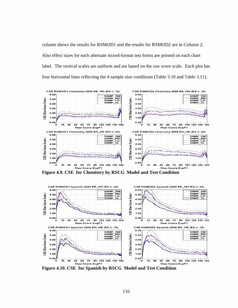
116
column shows the results for RSMOD1 and the results for RSMOD2 are in Column 2.
Also effect sizes for each alternate mixed-format test forms are printed on each chart
label. The vertical scales are uniform and are based on the raw score scale. Each plot has
four horizontal lines reflecting the 4 sample size conditions (Table 3.10 and Table 3.11).
Figure 4.9. CSE for Chemistry by RSCG Model and Test Condition
Figure 4.10. CSE for Spanish by RSCG Model and Test Condition
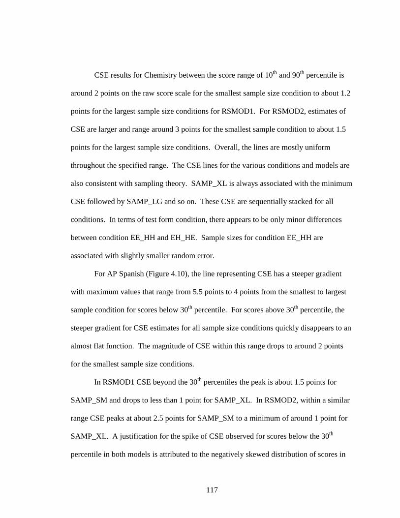
117
CSE results for Chemistry between the score range of 10th and 90th percentile is
around 2 points on the raw score scale for the smallest sample size condition to about 1.2
points for the largest sample size conditions for RSMOD1. For RSMOD2, estimates of
CSE are larger and range around 3 points for the smallest sample condition to about 1.5
points for the largest sample size conditions. Overall, the lines are mostly uniform
throughout the specified range. The CSE lines for the various conditions and models are
also consistent with sampling theory. SAMP_XL is always associated with the minimum
CSE followed by SAMP_LG and so on. These CSE are sequentially stacked for all
conditions. In terms of test form condition, there appears to be only minor differences
between condition EE_HH and EH_HE. Sample sizes for condition EE_HH are
associated with slightly smaller random error.
For AP Spanish (Figure 4.10), the line representing CSE has a steeper gradient
with maximum values that range from 5.5 points to 4 points from the smallest to largest
sample condition for scores below 30th percentile. For scores above 30th percentile, the
steeper gradient for CSE estimates for all sample size conditions quickly disappears to an
almost flat function. The magnitude of CSE within this range drops to around 2 points
for the smallest sample size conditions.
In RSMOD1 CSE beyond the 30th percentiles the peak is about 1.5 points for
SAMP_SM and drops to less than 1 point for SAMP_XL. In RSMOD2, within a similar
range CSE peaks at about 2.5 points for SAMP_SM to a minimum of around 1 point for
SAMP_XL. A justification for the spike of CSE observed for scores below the 30th
percentile in both models is attributed to the negatively skewed distribution of scores in

118
AP Spanish that resulted in sparse data at the lower score range. In terms of the EE_HH
and EH_HE conditions there appears to be no noticeable difference between RSMOD1
and RSMOD2 as illustrated by the CSE plots.
Plausible conclusions based on visual inspections of CSE between RSMOD1 and
RSMOD2 are that the equating functions based on RSMOD1 were associated with less
random variation at similar sample sizes compared to equating functions for RSMOD2.
This conclusion was consistent for both AP Chemistry and AP Spanish. Another
conclusion is that there are no differences in CSE between EE_HH and EH_HE within
each model.
Are there differences between RSMOD1 and RSMOD2 in terms of conditional equating
bias?
Results of equating accuracy measured using bias for RSMOD1 and RSMOD2
are displayed in Figure 4.11 and Figure 4.12. These figures are arranged using the same
outline described for CSE. For the bias plots the additional feature on each plot are two
horizontal lines on the vertical scale at .5 and -.5 that represent the criterion of difference
that matter (DTM).
For Chemistry, aggregated results of the bias estimates comparing RSMOD1
(Column 1) and RSMOD2 (Column 2) across the various samples for condition EE_HH
appeared to favor RSMOD1 as being less biased. That is bias functions in RSMOD1 are
closer together and predominantly lie within the DTM criterion boundary for scores
between the 10th and 90th percentiles. On the other hand, the lines representing bias
estimates for RSMOD2 also predominantly lie within the DTM range with the exception

119
of SAMP_MD condition. For the EH_HE condition, the lines representing bias estimate
for both RSMOD1 and RSMOD2 showed a slight inflection beyond the upper limits of
the DTM indicating a plausible overestimation of the equating function along the middle
of the score scales.
Figure 4.11. Bias for Chemistry by RSCG Model and Test Condition
In Spanish (Figure 4.12), estimates of bias in RSMOD1 for both EE_HH and
EH_HE are completely clustered together with the exception of the SAMP_SM
condition. The bias functions for these conditions lies entirely within the DTM boundary
for scores beyond the 30th percentile. Conversely, for RSMOD2, the trend lines for bias
are distinctive for the most part and predominantly lie within the DTM boundary for
scores beyond the 30th percentile. Conditions EE_HH and EH_HE yielded similar
results. A plausible explanation for the similarity in terms of bias between the EE_HH
and EH_HE conditions in Spanish is that the effect sizes of mixed-format difficulty in
120
both conditions were of similar range .24 and .15 for EE_HH and EH_HE respectively.
This compared to .15 and .03 for EE_HH and EH_HE in Chemistry.
Figure 4.12. Bias for Spanish by RSCG Model and Test Condition
Visual comparison of bias for the RSMOD1 and RSMOD2 shows that equating
functions from RSMOD1 were slightly less biased when compared to the equating
functions from RSMOD2. In terms of test form conditions, conclusions are different
across the two subjects. In AP Chemistry, EE_HH in both models are associated with
less bias compared to EH_HE. For AP Spanish, there appeared to be no detectable visual
difference in the aggregate bias estimates between RSMOD1 and RSMOD2.
Are there differences between model 1 and model 2 in terms of overall precision and
accuracy (RMSE)?
Overall equating precision and accuracy was estimated as the sum of the squared
bias and CSE variance. Conditional estimates of RMSE are presented in Figure 4.13 and

121
Figure 4.14. Each plot in the figures shows the conditional estimates of the RMSE for
each of the sampling conditions and score points. The labels on the RMSE lines
represent the four AP cut scores used to report final AP grades. The RMSE results for
Chemistry indicated that RSMOD1 across all sample size conditions are associated with
lower total equating error compared to RSMOD2 at similar levels of sample size. For the
condition EE_HH the range of RMSE in RSMOD1 varies from about 2 points for the
smallest sample size to about 1.2 points for the largest sample size condition. In
RSMOD2 these estimates ranged from around 3 to 2 points for the smallest to largest size
condition, respectively. The estimates for the EH_HE conditions were slightly higher but
consistent with the pattern described for EE_HH condition.
Figure 4.13. RMSE for Chemistry by RSCG Model and Test Condition
The RMSE results for Spanish (Figure 4.14) were also consistent with the
findings reported for Chemistry. RSMOD1was more accurate, the estimated RMSE

122
values ranging from 1.2 to .8 points for scores at the 30th percentile and above. In
RSMOD2 the estimated RMSE values ranged from 2 to 1 point for scores at the 30th
percentile and above. There appeared to be a trivial difference between condition
EE_HH and EH_HE with EE_HH being slightly more accurate.
Figure 4.14. RMSE for Spanish by RSCG Model and Test Condition
A general conclusion based on final estimate of RMSE for all conditions across
the two subjects showed that more than 95% of total equating error was associated with
random error. RSMOD1 was associated with less total error compared to RSMOD2 for
all conditions.
What are the minimum sample requirements for each model to ensure acceptable levels
of equating precision and accuracy?
Results from classification consistency at the five AP grade levels and the
probability of classification inconsistency at the critical 2/3 cutoff score were analyzed to
123
provide empirical recommendations in terms of adequate sample sizes in RSMOD1 and
RSMOD2. Table B.1 through Table B.6 of Appendix B show the proportion of
classification consistency by sample size condition. Only the last two columns of these
tables (RSMOD1 and RSMOD2) were interpreted relative to Research Question 1.
Proportions of classification consistency (as described in Chapter III) provide us
with empirical estimates of relative decision accuracy for each model across the five AP
grades. For example in Table B.1, where Row 1 in RSMOD1 is interpreted as an average
based on 500 bootstrap replications, examinees were classified into the same grade as did
their classification from the SG criterion 94% of the time. For RSMOD2 the rate of
consistency was slightly lower at 91%. An important statistic in these tables is the
minimum rate of agreement from 500 bootstrap replications of the data and analysis
under each model. For RSMOD1 the worst rate of agreement for condition EE_HH
ranged from 78% for SAMP_SM to 81% for SAMP_XL in RSMOD1 compared to 67%
and 75% for the SAMP_SM and the SAMP_XL conditions respectively in RSMOD2.
To address the issue of minimum sample size, the operational question was “What
is the probability to observe a given rate of classification inconsistency at the 2/34 cut?”
That is, what is the probability that a single sample that is selected for equating will
erroneously classify examinees as having an equated AP grade of 3 instead of a 2 and 2
instead of 3. Results of the empirical probability of classification inconsistency are
shown in Figure 4.15 and Figure 4.16. Each figure has the same format as those for CSE.
4 2/3 cut was selected as the critical decision point following the recommendation by the American Council on Education that colleges and universities grant credit and/or placement into higher-level courses to entrants with AP Exam grade of 3 or higher

124
The vertical axis scale represents the cumulative probability and the horizontal axis scale
is the proportion of classification inconsistency. The vertical line on the horizontal axis
indicates the 5% classification inconsistency marker at the 2/3 cut. The two horizontal
lines on the vertical axis show the 95th and 99th percentile markers respectively.
Figure 4.15. Probability of Classification Inconsistency at the 2/3 AP Cut Chemistry
Results in Chemistry for condition EE_HH show that there is a less than 1%
chance out of 500 bootstrap samples to select a sample that will result in a 5% or greater
rate of classification inconsistency in any sample size condition in RSMOD1. In
RSMOD2, the probability of selecting a sample that would result in 5% or more
classification inconsistency at the 2/3 cut is slightly greater than 1% for SAMP_LG and
SAMP_XL. This probability increased to about 6% for SAMP_MD and SAMP_SM.

125
Figure 4.16. Probability of Classification Inconsistency at the 2/3 AP Cut Spanish
Results for AP Spanish indicated the probability of selecting a sample that would
result in classification inconsistency of 5% or greater is less than 1% in RSMOD1 for
condition EE_HH. In RSMOD2 the probability was slightly higher than 1% for
SAMP_XL and SAMP_LG and between 5 and 6% for SAMP_MD and SAMP_SM.
Results for the condition EH_HE were consistent with those reported for the EE_HH
condition across both models.
4.2.1. Overall Summary
Overall summary results of RSMOD1 and RSMOD2 were compared using
weighted averages of CSE, bias and RMSE and classification inconsistency. This
provided a single summary statistic with which to concisely compare the two models.
Table 4.9 through Table 4.12 and Figure 4.17 through Figure 4.20 contain the complete
summary of weighted averages for the three evaluation criteria on all equating designs.
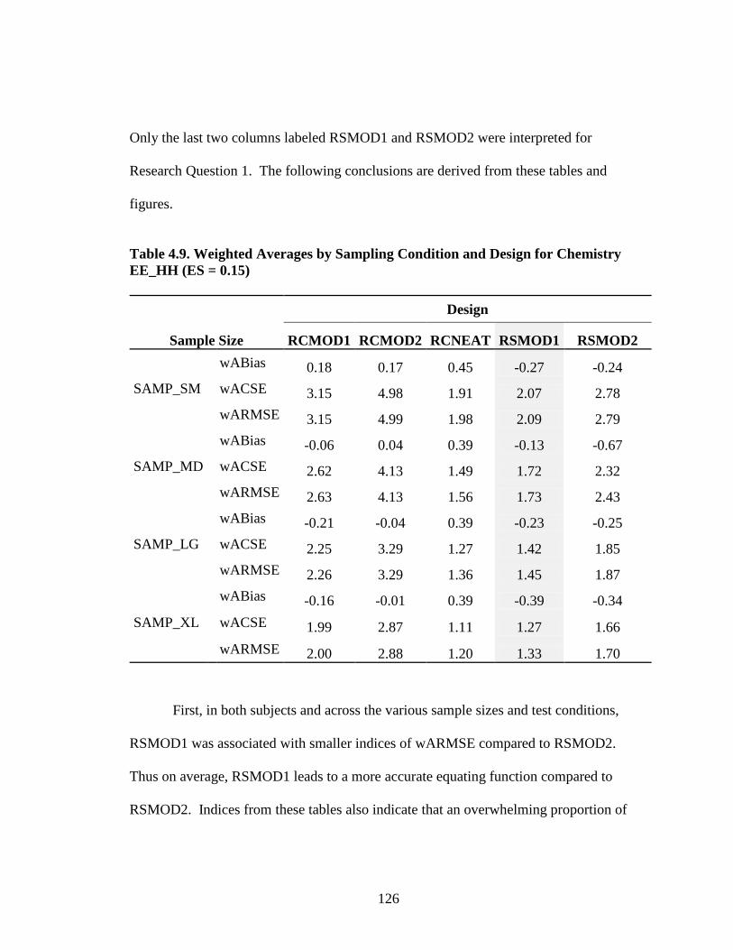
126
Only the last two columns labeled RSMOD1 and RSMOD2 were interpreted for
Research Question 1. The following conclusions are derived from these tables and
figures.
Table 4.9. Weighted Averages by Sampling Condition and Design for Chemistry EE_HH (ES = 0.15)
Sample Size
Design
RCMOD1 RCMOD2 RCNEAT RSMOD1 RSMOD2
SAMP_SM
wABias 0.18 0.17 0.45 -0.27 -0.24 wACSE 3.15 4.98 1.91 2.07 2.78 wARMSE 3.15 4.99 1.98 2.09 2.79
SAMP_MD
wABias -0.06 0.04 0.39 -0.13 -0.67 wACSE 2.62 4.13 1.49 1.72 2.32 wARMSE 2.63 4.13 1.56 1.73 2.43
SAMP_LG
wABias -0.21 -0.04 0.39 -0.23 -0.25 wACSE 2.25 3.29 1.27 1.42 1.85 wARMSE 2.26 3.29 1.36 1.45 1.87
SAMP_XL
wABias -0.16 -0.01 0.39 -0.39 -0.34 wACSE 1.99 2.87 1.11 1.27 1.66 wARMSE 2.00 2.88 1.20 1.33 1.70
First, in both subjects and across the various sample sizes and test conditions,
RSMOD1 was associated with smaller indices of wARMSE compared to RSMOD2.
Thus on average, RSMOD1 leads to a more accurate equating function compared to
RSMOD2. Indices from these tables also indicate that an overwhelming proportion of

127
total equating error form both models was made up of random equating error measured
by CSE.
Table 4.10. Weighted Averages by Sampling Condition and Design for Chemistry 2009 EH_HE (ES = 0.03)
Sample Size
Design
RCMOD1 RCMOD2 RCNEAT RSMOD1 RSMOD2
SAMP_SM
wABias 0.15 0.17 1.23 0.54 0.54 wACSE 3.28 5.09 1.99 2.16 2.84 wARMSE 3.28 5.10 2.36 2.25 2.90
SAMP_MD
wABias -0.04 0.01 1.20 0.67 0.07 wACSE 2.72 4.25 1.56 1.79 2.36 wARMSE 2.73 4.26 1.99 1.93 2.36
SAMP_LG
wABias -0.17 -0.02 1.25 0.55 0.53 wACSE 2.35 3.39 1.33 1.48 1.90 wARMSE 2.36 3.39 1.85 1.59 1.99
SAMP_XL
wABias -0.17 0.03 1.20 0.38 0.46 wACSE 2.05 2.98 1.16 1.31 1.68 wARMSE 2.06 2.98 1.69 1.37 1.75
Second, comparative analyses within each test subject (Chemistry and Spanish)
revealed some nominal differences with regard to the average bias between conditions
EE_HH and EH_HE in each subject. In AP Chemistry, wABias for both EE_HH and
EH_HE were about the same in both models. For AP Spanish, on average, RSMOD2
was associated with less bias than RSMOD1. Again these differences were trivial
compared to the differences observed between the models for wACSE.
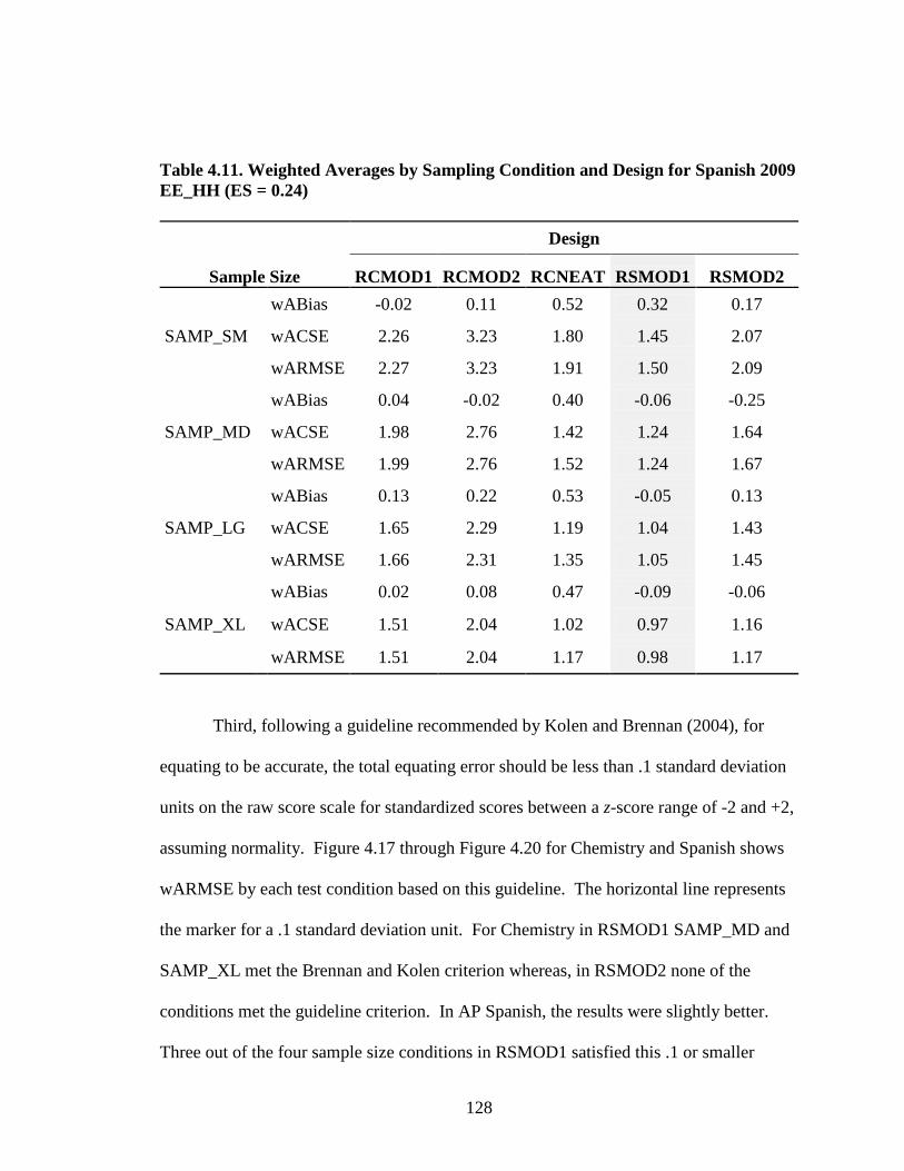
128
Table 4.11. Weighted Averages by Sampling Condition and Design for Spanish 2009 EE_HH (ES = 0.24)
Sample Size
Design
RCMOD1 RCMOD2 RCNEAT RSMOD1 RSMOD2
SAMP_SM
wABias -0.02 0.11 0.52 0.32 0.17 wACSE 2.26 3.23 1.80 1.45 2.07 wARMSE 2.27 3.23 1.91 1.50 2.09
SAMP_MD
wABias 0.04 -0.02 0.40 -0.06 -0.25 wACSE 1.98 2.76 1.42 1.24 1.64 wARMSE 1.99 2.76 1.52 1.24 1.67
SAMP_LG
wABias 0.13 0.22 0.53 -0.05 0.13 wACSE 1.65 2.29 1.19 1.04 1.43 wARMSE 1.66 2.31 1.35 1.05 1.45
SAMP_XL
wABias 0.02 0.08 0.47 -0.09 -0.06 wACSE 1.51 2.04 1.02 0.97 1.16 wARMSE 1.51 2.04 1.17 0.98 1.17
Third, following a guideline recommended by Kolen and Brennan (2004), for
equating to be accurate, the total equating error should be less than .1 standard deviation
units on the raw score scale for standardized scores between a z-score range of -2 and +2,
assuming normality. Figure 4.17 through Figure 4.20 for Chemistry and Spanish shows
wARMSE by each test condition based on this guideline. The horizontal line represents
the marker for a .1 standard deviation unit. For Chemistry in RSMOD1 SAMP_MD and
SAMP_XL met the Brennan and Kolen criterion whereas, in RSMOD2 none of the
conditions met the guideline criterion. In AP Spanish, the results were slightly better.
Three out of the four sample size conditions in RSMOD1 satisfied this .1 or smaller

129
criterion. The one exception was SAMP_SM in RSMOD1. In RSMOD2 only
SAMP_XL met this requirement.
Table 4.12. Weighted Averages by Sampling Condition and Design for Spanish 2009 EH_HE (ES = 0.15)
Sample Size
Design
RCMOD1 RCMOD2 RCNEAT RSMOD1 RSMOD2
SAMP_SM
wABias -0.04 0.16 0.89 0.65 0.45 wACSE 2.49 3.26 2.02 1.60 2.13 wARMSE 2.49 3.26 2.24 1.74 2.19
SAMP_MD
wABias 0.03 -0.01 0.80 0.24 0.06 wACSE 2.13 2.82 1.62 1.35 1.71 wARMSE 2.13 2.82 1.85 1.38 1.72
SAMP_LG
wABias 0.16 0.24 0.95 0.25 0.40 wACSE 1.81 2.34 1.39 1.14 1.46 wARMSE 1.82 2.35 1.72 1.17 1.53
SAMP_XL
wABias 0.04 0.04 0.89 0.21 0.24 wACSE 1.60 2.08 1.20 1.04 1.21 wARMSE 1.60 2.08 1.53 1.06 1.24
Finally, empirical evidence presented so far supported the alternate hypothesis
that RSMOD1 would lead to more accurate equating compared to RSMOD2 for mixed-
format test. Results from AP Chemistry and AP Spanish each independently supported
this claim. Conclusion with regard to conditions EE_HH and EH_HE showed that in
both subjects condition EE_HH was associated with less equating error compared to
EH_HE. The magnitude of the differences between the two conditions was directly

130
related to sample size. The differences were most evident for SAMP_SM and trivial for
SAMP_XL.
Figure 4.17. Summary of wARMSE for Chemistry 2009 EE_HH
Figure 4.18. Summary of wARMSE for Chemistry 2009 EH_HE
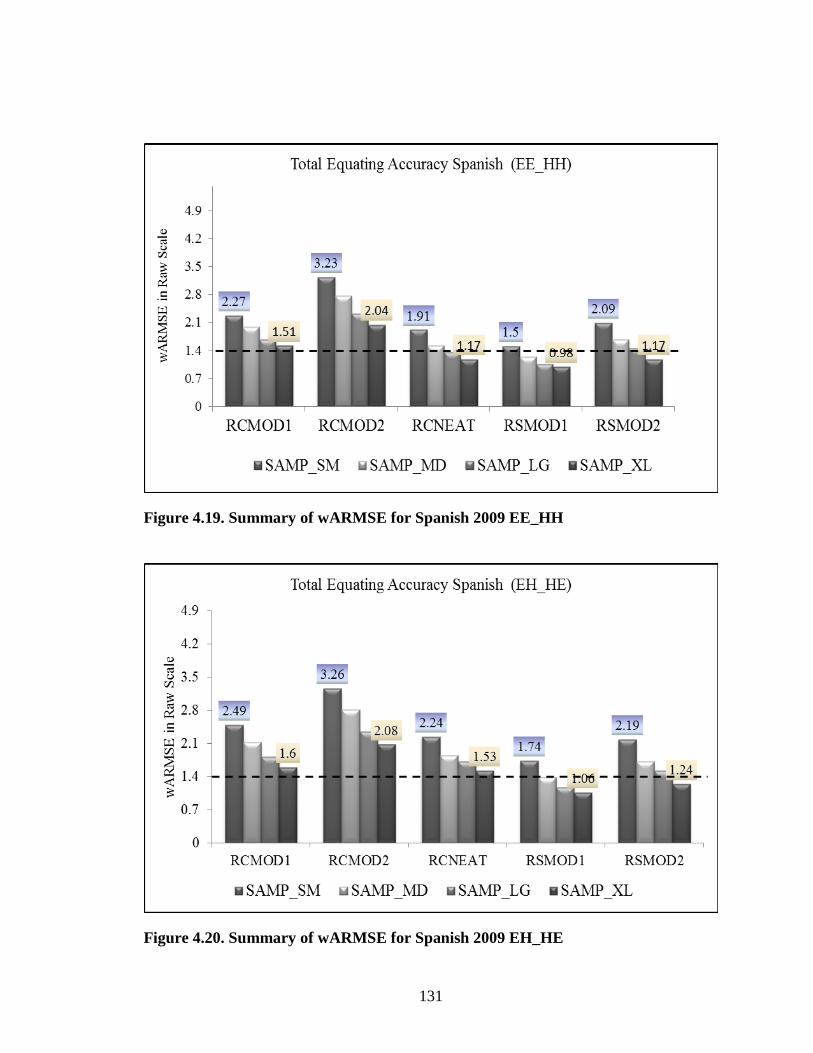
131
Figure 4.19. Summary of wARMSE for Spanish 2009 EE_HH
Figure 4.20. Summary of wARMSE for Spanish 2009 EH_HE
132
4.3. Results—Research Question 2
Problem 2: How does the random stratified cluster groups (RSCG) design compare to a
NEAT design with MC only anchor items and a random cluster design?
Research Question 2 addressed two relevant issues. The first issue was to
compare equating accuracy of mixed-format test between RSCG designs and a NEAT
design with MC only common items. The obvious limitation of this methodology is that
a NEAT design with MC only items completely ignores the fundamental components of
mixed-format test dimensionality. Thus, results presented for the NEAT design should
be interpreted cautiously. The second issue addressed in Research Question 2 was to
provide empirical evidence whether stratification on a covariate leads to any additional
benefits over simple random cluster sampling.
Results described in this section were based on the research design shown in
Figure 3.6. The hypothetical population in both AP subjects was modified to
accommodate each data collection design. In the NEAT design, the 500 bootstrap
replications were done by sampling from two nonequivalent populations created from the
examinee data from 2009. In the case of the random cluster (RC) designs, 500 bootstrap
replications were sampled directly from the 2009 examinee dataset to mimic Model 1 and
Model 2 described for RSCG. For each design the sampling rates were modified to
reflect the respective sampling frames. The main evaluation criteria of CSE, bias and
RMSE in addition with classification consistency were used to summarize results.
Results from RSMOD1 in the RSCG design are highlighted in the comparisons following
133
the conclusions from Research Question 1 where it was established that RSMOD1 was
more accurate compared to RSMOD2.
4.3.1. Equating Accuracy—RSCG vs. RCNEAT—Chemistry
Summary results comparing the RSCG designs with the RCNEAT design are
shown in Figure 4.21 and Figure 4.22. Results for RSCG design are displayed in Column
1 of the 2x2 figure. Comparative results for RCNEAT are displayed in Column 2. Row
1 show results for EE_HH condition and results for EH_HE condition are shown in Row
2. Results of CSE for RSCG in both designs ranges from 2 points for the smallest sample
condition to just greater than1 point for the largest sample conditions along the entire
score range. CSE in RCNEAT show a slight deep in the function for scores around the
mean. CSE is slightly below 2 for the largest sample condition to slightly below 1for the
largest sample size condition. These results were consistent across the two test
conditions. A summary of weighted CSE statistics are shown in Table 4.9 and Table
4.10.
With regard to conditional bias estimates, results displayed in Figure 4.22 shows
that for condition EE_HH, the bias statistics for the RCNEAT design on all sample size
conditions were identical but irregular along the score scale. These bias functions lie
predominantly within the DTM criterion boundary. In RSMOD1, bias functions for all
conditions form a series of straight lines that are not completely clustered together.
However, all of the bias trends lie entirely within the DTM criterion for most of the scale
scores.

134
Figure 4.21. CSE for RSCG vs. RCNEAT—Chemistry
Figure 4.22. Bias for RSCG vs. RCNEAT—Chemistry

135
Summary results of wABias shown in Table 4.9 and Table 4.10 indicated that on
average, the NEAT design overestimated the baseline equating functions by .45 points for
the smallest sample size condition to .39 for the largest sample size. On the other hand,
RSMOD1 was shown to underestimate the bias function by an average of -.27 for the
smallest sample size condition to -.39 for the largest sample size condition.
For condition EH_HE equating functions based on RCNEAT were associated
with significant rates of bias based on the DTM criterion. The bias functions were
distinctively irregular and entirely outside of the DTM boundary. Overall wABias
estimates from Table 4.9 and Table 4.10 confirm that on average the equating functions
were overestimated using the NEAT design by as much as 1.23 points for the smallest
sample condition to 1.16 points for the largest sample conditions. In RSMOD1, average
bias overestimation of the equating function ranged from .54 to .38 for SAMP_SM to
SAMP_XL respectively.
A comparison of empirical results of total equating accuracy for RSMOD1 and
RCNEAT in Chemistry produced mixed findings across the two test form conditions.
Results of wARMSE for condition EE_HH suggested that RCNEAT was on average
more accurate when compared to RSMOD1. For the largest sample size conditions,
wARMSE were 1.20 and 1.33 for NEAT and RSMOD1 respectively.
For condition EH_HE on the other hand, wARMSE estimates showed that
RSMOD1 on average was more accurate compared to RCNEAT designs. The average
estimates for SAMP_XL were 1.37 in RSMOD1 and 1.69 in RCNEAT. A direct cause of
these differences in the conclusion was attributed to the wider disparity of bias between
136
the two test conditions in the RCNEAT design. For example results of wABias estimates
for SAMP_XL increased from .39 for condition EE_HH to 1.20 for condition EH_HE. A
plausible explanation for the spike in bias in condition EH_HE could be related to the
fact that the NEAT design with MC only anchor items failed to model the difference in
test form difficulty attributed to changes in the covariance structure between MC and CR
items when easier MC items were paired with more difficult CR items to create the
composite form.
4.3.2. Equating Accuracy—RSCG vs. RCNEAT—Spanish
Results of CSE, bias and RMSE for AP Spanish are shown in Figure 4.23 and
Figure 4.24. For scores above the 30th percentile, CSE estimates in RSMOD1 were
slightly lower than those for RCNEAT design. This trend was consistent for condition
EE_HH and EH_HE. Summary estimates of wACSE from Table 4.11 for condition
EE_HH shows the average wACSE in RSMOD1 ranged from 1.45 for SAMP_SM to .97
for SAMP_XL compared to 1.80 and 1.02 for SAMP_SM to SAMPXL in RCNEAT.
Results for EH_HE condition (Table 4.12) shows wACSE ranged from 1.60 for
SAMP_SM to 1.04 for SAMP_XL in RSMOD1 and 2.02 for SAMP_SM to 1.20 for
SAMP_XL in RCNEAT design. Thus, for Spanish RCNEAT was associated with more
random error compared to RSMOD1.
Conditional bias estimates from both designs (Figure 4.24) shows marked
differences in conditional bias between the two designs and across test form conditions.
Conditional bias functions for condition EE_HH in RSMOD1 across all sample
conditions except for SAMP_SM were clustered together in one smooth function for

137
scores above the 30th percentile. These bias functions lied entirely within the DTM
boundary.
Figure 4.23. CSE for RSCG vs. RCNEAT—Spanish
The same was evident for condition EH_HE. In RCNEAT design, conditional
bias functions were stacked together in an irregular pattern that fluctuated in and out of
the DTM boundary. For EH_HE condition, the fluctuations were more pronounced with
most of the functions lying outside of the DTM boundaries. The minor exceptions were
for scores between 75 and 95 in which their bias was on the upper boundary of the DTM.
Comparison results of total equating accuracy presented in Table 4.11 for Spanish
confirms that RSMOD1 was more accurate compared to RCNEAT design. These
findings were consistent across the two test conditions. For condition EE_HH, equating
functions based on RSMOD1 were on average 21% to 16% more accurate when
compared to RCNEAT for SAMP_SM and SAMP_XL respectively. In condition
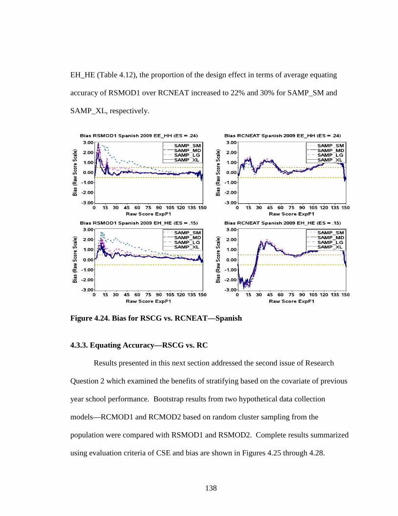
138
EH_HE (Table 4.12), the proportion of the design effect in terms of average equating
accuracy of RSMOD1 over RCNEAT increased to 22% and 30% for SAMP_SM and
SAMP_XL, respectively.
Figure 4.24. Bias for RSCG vs. RCNEAT—Spanish
4.3.3. Equating Accuracy—RSCG vs. RC
Results presented in this next section addressed the second issue of Research
Question 2 which examined the benefits of stratifying based on the covariate of previous
year school performance. Bootstrap results from two hypothetical data collection
models—RCMOD1 and RCMOD2 based on random cluster sampling from the
population were compared with RSMOD1 and RSMOD2. Complete results summarized
using evaluation criteria of CSE and bias are shown in Figures 4.25 through 4.28.

139
Figure 4.25. CSE for RSCG vs. RC—Chemistry
Figure 4.26. Bias for RSCG vs. RC—Chemistry

140
Figure 4.27. CSE for RSCG vs. RC—Spanish
Figure 4.28. Bias for RSCG vs. RC—Spanish

141
These 2x2 figures show the results for RSCG in Column 1 and RC in Column 2.
Again Row 1 presents the results for condition EE_HH and Row 2 for condition EH_HE.
Discussions of results were dominated by comparisons between RSMOD1 and RCMOD1
because they were associated with smaller amounts of equating error in each design.
4.3.4. Equating Accuracy—RSCG vs. RC—Chemistry
CSE estimates between RSMOD1 and RCMOD1 show obvious differences in the
magnitude of random error (Figure 4.25). The gradient of CSE for RSMOD1 for
condition EE_HH were flat for most of the score scale and ranged from 2 points for
SAMP_SM to about 1 point for SAMP_XL. CSEs for condition EH_HE had a similar
shape though the random errors were slightly larger. In RCMOD1 for condition EH_HE
conditional random error functions produced a curved shape with maximum estimates
around the median scores. The range of CSE is from 3 points to 2 points for SAMP_SM
and SAMP_XL. Similar interpretations were drawn from condition EH_HE in
RCMOD1.
Results of conditional bias displayed in Figure 4.25 indicated an almost straight
line representing bias for RCMOD1 that were entirely within the DTM boundary in both
EE_HH and EH_HE conditions. Conditional bias functions for RSMOD1were not
entirely as smooth compared to those in RCMOD1 but were predominantly at the lower
bound of the DTM criterion for condition EE_HH. Conditional bias functions for
condition EH_HE in RSMOD1 showed a slight concavity for most of the scale and lie
predominantly along the upper bound of the DTM criterion. A reasonable explanation of
the almost zero bias in the RCMOD1 was due to a larger design effect in which the

142
sampling frame for RCMOD1 was equal to the population when compared to RSMOD1
in which the sampling frame only captured 58% of the population elements.
Summary findings of equating accuracy suggested that RSMOD1 was on average
more accurate when compared to RCMOD1 for both test conditions EE_HH and
HEH_HE (Table 4.9 and Table 4.10). The gain in equating accuracy by sampling from
the stratified matrix based on average school AP grade as opposed to simple random
cluster is about 34%. In condition EE_HH the average RMSE in RSMOD1 for
SAMP_SM is 2.09 and 1.33 for SAMP_XL. For the same condition in RCMOD1 the
average estimates were 3.15 and 2.00 for SAMP_SM to SAMP_XL. Average estimates
for condition EH_HE were slightly higher ranging from 2.25 and 1.37 for SAMP_SM
and SAMP_XL in RSMOD1 and from3.28 to 2.06 for SAMP_SM and SAMP_XL in
RCMOD1.
4.3.5. Equating Accuracy—RSCG vs. RC—Spanish
Results in Spanish comparing RSMOD1 and RCMOD1 in terms of CSE and bias
were consistent with those reported for Chemistry. Figure 4.27 and Figure 4.28 display
the conditional summaries based on these evaluation criteria. Most noticeable were the
differences in CSE between RSMOD1 and RCMOD1 in both conditions.
In terms of conditional Bias, despite the sampling advantage of RCMOD1 over
RSMOD1, the differences in the bias term were at best marginal in favor of RCMOD1.
Results in Figure 4.28 showed no apparent differences between condition EE_HH and
EH_HE.

143
Total equating accuracy also confirmed the findings reported for Chemistry
(Table 4.11 and Table 4.12). For condition EE_HH in Spanish, RSMOD1 resulted in on
average 34% more accurate equating conversions compared to RCMOD1. In condition
EH_HE, the estimated benefits of RSMOD1 dropped slightly to 32%. Total equating
error in RSMOD1 estimated using wARMSE, for SAMP_SM was 1.5 and .98 for
SAMP_XL. In RCMOD1 the average values were 2.27 and 1.51 for SAMP_SM to
SAMP_XL. The wARMSE estimates for condition EH_HE were slightly higher in both
designs.
4.3.6. Summary for Research Question 2
Empirical results presented provide clear conclusions on the two main issues
addressed by Research Question 2. First, results from AP Chemistry and AP Spanish
both suggested that RSCG design was associated with less equating error for mixed-
format test compared to a RCNEAT design with MC only common items. The
magnitude of design effect between RSCG and RCNEAT varied across the two test
conditions evaluated in this research. For condition EE_HH in Chemistry, RCNEAT
design appeared to be on average more accurate when compared to the RSCG design.
This result is not necessarily an endorsement of the NEAT design with MC only anchor
items over RSCG design for mixed-format test. A major weakness of the NEAT design
with MC only anchor item was that the anchor was a part anchor not a mini version of the
two full-length test forms. In addition, technical dimensionality aspects of mixed-format
test (e.g. differential covariance patterns over time) in such instances are essentially
ignored.

144
For test form condition EH_HE, results in both Chemistry and Spanish support
the alternate hypothesis that the RSCG design was more accurate compared to RCNEAT
design with MC only anchor items. Figures 4.17 through 4.20 present summary results
of overall equating accuracy based on Kolen and Brennan’s recommendation on equating
precision.5 The horizontal line is the marker at 0.1 standard error of equating. Results
show that RSMOD1 has the most sampling conditions with total equating error less than
0.1. The one exception in which the RCNEAT design seems to outperform RSMOD1 is
in Chemistry EE_HH. Plausible implications of this finding will be discussed in Chapter
V.
The second conclusion derived from these results was that stratification on
previous year AP school performance provided an improvement in terms of overall
equating accuracy over the simple random cluster sampling in the EG design. The two
models from the RSCG design consistently outperformed the two models based on RC.
Equating functions from RSMOD1 were associated with the least amount of equating
error (Figure 4.17 through Figure 4.20).
Finally, classification consistency indices (see Appendix B) confirm these results
were associated with higher rates of consistency within each condition. Rates of
consistency varied by designs and sample size across all test conditions. For a majority
of the conditions results from RSMOD1 were the most consistent with average
5 For random groups design under normality assumption the standard error of equating between z-score of -2 and +2 was shown to be less than .1 when sample size was over 1500 per form for equipercentile equating (Kolen & Brennan, 2004, p. 288).

145
consistency rates in the range of 92% to 94% for SAMP_SM to SAMP_XL. Results
from RCMOD2 were the least consistent with average rates ranging from 83% to 91%.
4.4. Results—Research Question 3
How much precision and accuracy is gained when the stratification variable is based on
more than one year of school aggregated data to predict subsequent year equivalent
stratified cluster of schools?
In Research Question 3, the goal was to evaluate the gains in overall equating
accuracy for the RSCG designs when the covariate of average school performance was
based on two previous years (e.g. 2008 and 2009) to create the equivalent groups
sampling frame for a subsequent (2010) equating. Experimental test forms created from
the 2010 data were used to equate the alternate mixed-format test forms.
Bootstrap summaries of CSE, bias and RMSE did not show any improvements in
overall equating accuracy for both subjects. Actual results of weighted averages
presented in Table 4.13 and Table 4.14, contrary to anticipated findings showed that the
stratification frame based on 2008 and 2009, data on average, did worse than results
based on 2008 stratification. In Chemistry for condition EE_HH wARMSE ranges from
2.42 SAMP_SM to 1.45 SAMP_XL in RSMOD1 for 2010 compared to 2.09 SAMP_SM
to 1.33 SAMP_XL in RSMOD1 for 2009. In Spanish, the differences in wARMSE
between the stratification frameworks for condition EE_HH ranges from 1.78 SAMP_SM
to 1.13 SAMP_XL in RSMOD1 for 2010 compared to 1.5 SAMP_SM to .98 SAMP_XL
in RSMOD1 for 2009.
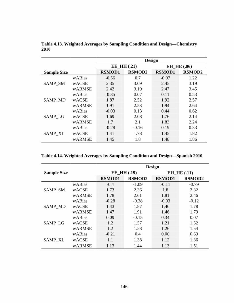
146
Table 4.13. Weighted Averages by Sampling Condition and Design—Chemistry 2010
Sample Size
Design EE_HH (.21) EH_HE (.06)
RSMOD1 RSMOD2 RSMOD1 RSMOD2
SAMP_SM wABias -0.56 0.7 -0.07 1.22 wACSE 2.35 3.09 2.45 3.19 wARMSE 2.42 3.19 2.47 3.45
SAMP_MD wABias -0.35 0.07 0.11 0.53 wACSE 1.87 2.52 1.92 2.57 wARMSE 1.91 2.53 1.94 2.64
SAMP_LG wABias -0.03 0.13 0.44 0.62 wACSE 1.69 2.08 1.76 2.14 wARMSE 1.7 2.1 1.83 2.24
SAMP_XL wABias -0.28 -0.16 0.19 0.33 wACSE 1.41 1.78 1.45 1.82 wARMSE 1.45 1.8 1.48 1.86
Table 4.14. Weighted Averages by Sampling Condition and Design—Spanish 2010
Sample Size Design EE_HH (.19) EH_HE (.11) RSMOD1 RSMOD2 RSMOD1 RSMOD2
SAMP_SM wABias -0.4 -1.09 -0.11 -0.79 wACSE 1.73 2.36 1.8 2.32 wARMSE 1.78 2.61 1.81 2.46
SAMP_MD wABias -0.28 -0.38 -0.03 -0.12 wACSE 1.43 1.87 1.46 1.78 wARMSE 1.47 1.91 1.46 1.79
SAMP_LG wABias 0.09 -0.15 0.34 0.07 wACSE 1.2 1.57 1.21 1.52 wARMSE 1.2 1.58 1.26 1.54
SAMP_XL wABias -0.21 0.4 0.06 0.63 wACSE 1.1 1.38 1.12 1.36 wARMSE 1.13 1.44 1.13 1.51

147
Post-hoc re-evaluation of the research design and data used in the study were
conducted and discussed in Chapter V in an attempt to provide justifications of the results
observed for Research Question 3.
148
CHAPTER V
DISCUSSION
The purpose of this dissertation is to investigate a practical equating issue
involving mixed-format test, using a stratification strategy to mimic a randomly
equivalent groups design. Specific focus of this dissertation was twofold. The first goal
was to present evidence on the use of a predictive stratification framework based on an
already available covariate to create equivalent groups. The second goal was to present
supporting evidence on an appropriate data collection design for mixed-format test
equating. This chapter provides summary discussions of the results presented in Chapter
IV. The discussions in Chapter V are organized in the following order. Section 5.1
presents an overview of the methodology adopted in this research. Section 5.2 presents
the major findings of each research problem. Section 5.3 provides discussion and
practical implications of the results. Section 5.4 outlines the limitations of the research
design and directions for future research.
5.1. Overview of Methodology
The purpose of this empirical study was to design and evaluate two predictive
sampling methodologies to collect data to equate mixed-format tests under the EG design
using observed score equating procedure. AP data in Chemistry and Spanish Language
were obtained covering a three year period. Resampling of the secondary data was then
used to evaluate the research questions described in Chapters I and III. The main

149
configuration of the stratified cluster sampling framework was based on two stratifying
variables—average school performance and school size from previous year(s) test data.
Examinee level test data from previous year was averaged within schools to create
a school level covariate. AP cutoff scores were then used to classify schools into five
distinct categories corresponding to the five AP grade levels. This constituted the main
covariate used to stratify schools into equivalent stratum. The second conditioning
variable was created by splitting the total number of examinees from each school into
five categories based on quintiles. These two variables were used to organize schools
into a 5x5 stratified sampling grid. The premise was that schools within a cell are
equivalent in terms of AP performance.
Probabilities proportionate to sample size were used to randomly select schools
into equating blocks based on two models. For RSMOD1, a single relatively small
sample of schools was selected from the equivalent stratified sampling frame. Examinees
from this sample were administered one of the alternate test forms and the other form was
administered to the larger population. Observed score equipercentile equating was then
used to equate scores from these two forms using examinees from the sample and those
left in the sampling frame.
In the second model, RSMOD2, two equivalent samples were selected from the
sampling frame and each administered one of the two alternate mixed-format test forms.
The population equating function of the alternate forms was then estimated using these
two random stratified equivalent samples. In addition to the RSCG data collection
designs, a random cluster NEAT (RCNEAT) design and two random clusters EG designs

150
(RCMOD1 and RCMOD2) similar to RSMOD1 and RSMOD2 were also evaluated.
Two other factors investigated other than the data collection designs were: two test
configurations in terms of relative difficulty of MC and CR items in a mixed-format test
and equating accuracy for different sample sizes.
To simulate the equating scenarios, experimental mixed-format test forms were
created by splitting a single test form into two alternate mixed-format tests based on
specified experimental conditions. Equating precision and accuracy were then evaluated
using a bootstrap re-sampling design. The criterion equating was based on a single group
equipercentile equating function using all examinees in the population. Results based on
500 bootstrap equating functions were summarized using three main summary indices—
CSE, bias, and RMSE. Also as a measure of reliability of the findings, classification
consistency index over the 500 replications was also estimated.
5.2. Summary of Major Findings
This section on summary of major findings is divided into 3 subsections following
the three main research questions. The research questions corresponding to each result
have been restated at the start of each new subsection. This research represents one of
the first attempts to investigate the accuracy of equating using a stratified sampling
methodology based on previous year school level covariates. Most research conducted
on mixed-format test under the EG relied on a random spiraling design at the student
level. Thus, findings from this research should not be directly compared with previous
findings from other mixed-format studies due to the difference in the methodology.
151
5.2.1. Research Question 1
Problem 1: How efficient is a sampling grid stratification design based on previous year
average AP school performance and school size to predict random clusters of school to
equate two alternate mixed-format test forms administered during a subsequent year?
1. Are there differences between model 1 and model 2 in terms of
a. Conditional equating precision measured by sampling variability of
equated scores?
b. Conditional equating Bias?
c. Overall equating precision and accuracy?
2. What are the minimum sample requirements for each model to ensure
acceptable levels of equating precision and accuracy?
First, for the sampling rate and test condition, RSMOD1 was associated with a
smaller amount of equating error compared to RSMOD2. Independent results in both
Chemistry and Spanish confirm this pattern. Empirical probabilities of incorrectly
classifying examinees at the 2/3 cut show that there was a less than 1% chance to
incorrectly classify 5% or more examinees in RSMOD1. With RSMOD2, the probability
to erroneously classify examinees at the 2/3 cut ranges from 1% to about 6%. Therefore,
empirical evidence from this dissertation suggests that RSMOD1 can be used with great
precision and accuracy to equate mixed-format test in AP exams.
The second major conclusion from this research is that a minimum sampling rate
of 7.5% (an average of 3675 examinees for Chemistry and 4310 examinees for Spanish)
was required in RSMOD1 to produce accurate estimated equated function for two

152
alternate mixed-format test using equipercentile equating. In RSMOD2, the minimum
sample rate required to achieve the same recommended amount of equating accuracy was
12.5% (an average of 6072 examinees for Chemistry and 7226 examinees for Spanish).
Third, results suggested a slight differential rate of equating accuracy in favor of
the EE_HH test condition in both subjects. The EE_HH condition was a combination of
relatively easier MC and CR items equated to a base form made of more difficult MC and
CR items or vice versa. The EH_HE condition was a combination of easier MC and
more difficult CR items on one form and more difficult MC with easier CR comprising
the second form. A plausible explanation of these differences in equating accuracy
between the two conditions could be attributed to the differential effect of the covariance
structure which was evident by the slight change in the correlation (Table 3.4 through
Table 3.7) between MC and CR items.
Fourth, an unanticipated conclusion from summaries of CSE, bias and RMSE
show that the estimated equated function for AP Spanish was associated with less
equating error compared to results from AP Chemistry. A probable explanation of these
findings was attributed to the effect of test difficulty on equating accuracy. Overall,
descriptive statistics from the two subjects showed the mean score in AP Chemistry was
substantially lower (61) compared to that of AP Spanish (85). Scores in AP Chemistry
were also associated with a higher standard deviation (33) compared to scores in Spanish
(25). Preliminary interpretation based on the data suggests that form difficulty of mixed-
format test in conjunction with higher variability of scores appeared to have a greater

153
effect on equating accuracy than the potential dimensionality differences between the two
subjects.
5.2.2. Research Question 2
1. How does the random stratified cluster group (RSCG) design model compare
to:
a. Random cluster NEAT design with MC only common items?
b. Simple random cluster design?
2. Are there significant differences as measured by equating bias?
3. What is the design effect between the RSCG and NEAT design, and RG and
RSCG design?
4. What is the impact of form difficulty combination of mixed-format test on
equating accuracy?
Research Question 2 compared RSCG designs against the NEAT design and a
random cluster design. The goal was to present justifiable evidence that RSCG design
would lead to a more accurate equating for mixed-format test and also that stratification
on a relevant covariate was an improvement over simple cluster sampling. Summary
findings on these two issues are discussed below.
RSMOD1 was associated with the smallest amount of equating error compared to
RCNEAT designs for all conditions except in Chemistry EE_HH where RCNEAT seem
to show slightly lower equating error estimates than RSMOD1. For condition EH_HE in
both subjects RSMOD1 outperformed RCNEAT design. The differences between
RSMOD1 and RCNEAT were substantially greater in Spanish where three out of the four

154
sampling rates had average standard equating error less than 0.1 compared to none of the
size condition in RCNEAT. These results are aligned with recent findings of research on
mixed-format equating by Rotou et al. (2011), Hagge and Kolen (2011), and unpulished
dissertations by Hagge (2010) and Cao (2008). Results from these studies concluded that
equating bias estimates were greater when a NEAT design with MC only anchor was
used to equate mixed-format test. The rate of bias was also shown to vary across content
areas as the correlation between MC and CR items changed.
With regard to the benefits of stratification, results comparing RSMOD1 with
RCMOD1 showed that for all conditions analyzed in this dissertation, equating functions
from RSMOD1 design were more accurate. None of the sampling conditions in the RC
models met the less than 0.1 standard error of equating requirement. Equating functions
estimated from RSMOD1 were on average 34% more accurate than their counterparts
obtained using RCMOD1. This gain in efficiency was directly attributed to design effect
of stratifying on previous year school AP rankings. These findings were consistent with
the benefits of sampling stratified cluster over simple random cluster reported in the
literature and discussed in Chapter II. Jaeger (1984) asserted that “The primary benefit
afforded by stratified sampling is increased statistical efficiency” (p. 67).
5.2.3. Research Question 3
Problem: How much precision and accuracy is gained when the stratification variable is
based on more than one year of school aggregated data to predict subsequent year
equivalent stratified cluster of schools.

155
1. What is the amount of increase in accuracy of predicting equivalent school
strata?
2. What is the amount of increase in overall equating error between the two
models?
3. Are these effects consistent across the different AP subjects?
Research Question 3 in which the stratified sampling grid was based on
aggregated data from two previous years (2008 and 2009) to create covariates to sample
equivalent schools for 2010 equating produced unexpected results. Overall weighted
averages of equating accuracy and precision from 2010 were higher than estimated errors
from 2009. These findings suggested that the RSCG model did worse when the sampling
grid was based on covariates from two previous years of data than when it was based on
data from a previous year. As a result of these unexpected findings, no definite
conclusions were made in this dissertation about Research Question 3. Probable
conclusions at this time are that these results might have been influenced by the particular
design or specific to AP exams. In an attempt to gain further insights as to the reason no
gains in equating accuracy and precision were noticed, three probable explanations are
offered below.
First, the proportion of sampling frame to population elements decreased from
58% in the 2009 sampling matrix to 52% in the 2010 sampling frame in Chemistry. This
increased the under-coverage error rate of the RSCG to predict equivalent schools for
2010 equating. For Chemistry the bias coverage error of average school AP raw score
was .22 in standard deviation units on the raw score scale. This translated to an average

156
error of 7 points for estimated school means. In Spanish, the average bias coverage error
was slightly lower at .15 in standard deviation units. The consequence was a
stratification framework based on a bias estimate of population covariate to classify
schools into equivalent strata.
A second plausible explanation is that averaging on two measurement occasions
might not provide a consistent estimate of each school’s actual classification. This,
coupled with the fact that each individual sampling frame was associated with significant
under-coverage error, made prediction of equivalent schools for 2010 equating more
difficult.
Finally, these findings might be a hint to an important empirical dilemma of how
far back is previous school data relevant to create a predictive stratified framework for
EG designs equating. Examinees and other school variables such as teachers, socio-
economic status of school and district are constantly changing and as such our stratified
framework might be more accurate with data from a single year out.
5.3. Practical Implications of Results
The framework of this dissertation was designed to address two main practical
issues. The first issue was to provide empirical evidence on the plausibility to accurately
equate mixed-format test constructed with the same content and statistical specifications
using an EG design with no common item. The second goal was to recommend a
preferred model and sample size for conducting EG equating. Practical implications of
this dissertation are presented following these two main goals.

157
5.3.1. Equating Mixed-Format Test Using EG Design
Results presented in this dissertation provide preliminary evidence to practitioners
of an alternative framework to equate mixed-format test that treats the confounding
dimensionality characteristics as a random variable. Overall results in Chemistry and
Spanish in RSCG design suggested that form difficulty had a greater impact on total
equating accuracy than potential dimensionality structure between the MC and CR items.
At this point, any attempts to generalize these results to other testing programs should be
done cautiously. Results also indicated that the use of MC only anchor items to equate
mixed-format test will lead to bias equating and is associated with significant validation
violations. This conclusion has been echoed in all studies on mixed-format equating
(Hagge & Kolen, 2011; Kim, Walker, & McHale, 2010; Rotou et al., 2011).
These findings even though localized to AP programs offer needed empirical
confirmatory evidence of a parsimonious but efficient alternative to equate mixed-format
test. This design is also associated with two cost saving features: (a) the covariates are
based on already existing data, and (b) the design makes use of the per cost savings
associated with sampling already existing clusters.
However, practitioners should interpret these results with caution as this is still
the early phase of building a validation argument for the RSCG design. More replication
studies in other large scale programs are required to build consistent evidence that could
be used to justify policy decisions.

158
5.3.2. Recommendation of Model and Sample Size
Results of total equating error in both AP subjects recommended a sampling rate
of at least 7.5% at the school level in RSMOD1 for equating errors less than 0.1 standard
deviation units. Some of the immediate practical implications associated with RSMOD1
are:
1. This model enables multiple forms of mixed-format test to be administered
during a test cycle without the risk of item exposure associated with a random
spiraling design or a NEAT design with trend scoring. In this multi-media era
where most human transactions involve a computer, the practice of offering
just a single test form is becoming obsolete. Thus RSMOD1 seems to have
the potentials to administer and accurately equate multiple mixed-format test
forms within a single year.
2. The framework of RSCG is fairly easy to implement and explain to
stakeholders. Unlike other complex data collection design such as trend
scoring, this model can be easily adopted and effectively implemented with
minimum personnel and financial resources.
5.4. Limitations of Research and Future Direction
This study represents the first experimentation in building a data collection
framework for equating mixed-format test under the RG design in an observational study.
The goal was to provide empirical evidence on two main issues: (a) accuracy of equating
mixed-format test using a stratification framework in an EG design, and (b) to make
recommendation of a model and sample size. The focus of this study was limited to these
159
two central issues. Interpretation of results and conclusions made from this dissertation
were bounded with the following limitations.
5.4.1. Potential Confounding Dimensionality of Mixed-Format Test
The issue of mixed-format dimensionality were not directly addressed in the
research design and results discussed. Research evidence and conclusions on mixed-
format dimensionality presented in Chapter II were equivocal. Messick (1993) reinforced
that what is purported in these studies as evidence of construct variance is merely what
Loevinger (1957) and Campbell and Fiske (1959) had defined as method variance. In
spite of the broader theoretical disagreements on how and what are the dimensions
represented in mixed-format test, there is no denying of a confounding dimensionality
aspect associated with mixed-format test. In a NEAT design these dimensionality
confounds are completely ignored especially when the anchor is made up of only MC
items. Regarding the effectiveness of equating using the NEAT design, Luecht and
Camara (2011) concluded that:
Even if the two CR traits were demonstrated to be invariant across years, the relationship between each CR trait and MC trait would need to be virtually identical for a composite of MC and CR traits to have any chance of holding up under any equating paradigm based only on MC items. . . . The method of equating/ calibration is not the issue. Rather, it is about the confounding of the dimensionality of the scales over time and the potential inability of the item or task linkages to maintain a consistent composite scale. (p. 12) In the RSCG design the relationship between the MC and CR in the population
was treated as a source of random variation in the equating design. No claim is made at

160
this time about the effect of variations in their relationship over time on the accuracy of
the RSCG model.
5.4.2. AP Data
Data used for this dissertation were from the AP exams in Chemistry and Spanish.
These two subjects are not representative of the entire range of AP content areas. AP
subjects are associated with specific characteristics in terms of the relative weights of
different item formats towards the composite score, number and type of CR items and
correlation between MC and CR. As a result, these variations in AP test characteristics
interpretation of results presented may not be readily generalized to other AP subjects.
The MC sections for all the data used in this dissertation were formula scored.
AP exams are no longer formula scored and therefore it is uncertain if these results will
directly translate to AP Chemistry and Spanish in which the MC section is right only
scored. The potential impact if any of formula scoring and differential weighting were
not investigated in this research.
5.4.3. Re-sampling Design
The main criticism of a re-sampling design framework in an equating study is that
the notion of truth is not tangible. A single group equipercentile relationship in the
population was established as the criterion with which sample estimates were compared.
Although this methodology has support in the literature (Harris & Crouse, 1993; Kolen &
Brennan, 2004; Livingston et al., 1990), its main limitation is that selection of a different
criterion is likely to produce somewhat different results. Harris and Crouse (1993) also
161
pointed that results based on such design are meaningful only to the extent that the
examinee groups are formed in a manner that is similar to how groups occur in practice.
5.4.4. Experimental Test Forms Design
Experimental alternate mixed-format test used in the hypothetical equating
scenarios were created from a single test form. The number of items that could go into
either form was restricted by the total items on the single form. The requirements of
same statistical and content specification for alternate mixed-format test were not fully
met. For AP Spanish the desired standardized effect size for EH_HE condition of a range
from 0 to .09 was not achievable given the fixed item pool. Thus, conclusions made on
the effect of test form difficulty and comparison of equating accuracy across the two AP
subjects are associated with wide variations in test form difficulty of the various
experimental mixed-format tests.
5.4.5. Future Research
There are many tangential issues associated with developing a framework for
equating mixed-format test. The scope of this dissertation did not nor could it address all
of the potential contentious issues. An important feature in mixed-format test is the fact
that the relationship between the items in the mixed-format test is often unpredictable
(i.e., not stable over time) and highly dependent on the type of items included in the
assessment and interactions between tasks and examinee characteristics. For this
research, the mixed-format item types were limited to MC and CR items. Other item
types are bound to be associated with different types of measurement requirements and
expectations. Therefore, there is a diverse but rich array of possibilities of future research
162
areas on this subject. The recommendations for future research listed below are direct
implications from this dissertation and they include:
1. Replication of results using generated data in other subject areas
2. Investigate the effect of differential correlation within mixed-format test on
equating accuracy.
3. Effect of mixed-format test form difficulty on equating accuracy.
4. Effect of mixed-format equating relationship invariance across different sub-
groups and over time.
5. Replication of this study using a multidimensional item response theory
framework. This will provide empirical evidence on the influence of test
dimensionality on the accuracy of mixed-format equating under the RSCG
designs.
5.4.6. Conclusion
Overall, results from this dissertation suggest that with large enough sample sizes,
the RSCG design based on a single covariate can be used to accurately equate mixed-
format test forms administered within the same testing cycle. Empirical evidence
endorses RSMOD1 as the viable choice that will result in accurate and precise equating
functions. Results also showed that the composition of mixed-format test forms in terms
of item difficulty combination have an effect on equating accuracy. The equating
function tended to be more accurate when item difficulties of the various sections were
similar and less accurate when the difficulty combinations of the sections were mixed.
163
A couple of unexpected findings from the dissertation occurred. First, equating
functions from Spanish were more accurate compared to those from Chemistry. The
implications of these results suggest that overall mixed-format difficulty had a greater
impact on equating accuracy than the covariance structure between the MC and CR
sections. Second, RSCG model was less accurate when the stratification frame was
based on aggregated data from two previous years compared to a single year. This
finding could be dependent on the particular choice of design factors and data. Or, more
importantly it could be an indication of how far back is historical data a relevant predictor
of current school configurations.

164
REFERENCES
American Educational Research Association, American Psychological Association, &
National Council on Measurement in Education. (1999). Standards for
educational and psychological tests. Washington, DC: American Educational
Research Association.
Ackerman, T. A., & Smith, P. L. (1988). A comparison of information provided by essay,
multiple-choice, and free-response writing tests. Applied Psychological
Measurement, 12(2), 117–128.
Bennett, R. E. (1993). On the meaning of constructed response. In R. E. Bennett & W. C.
Ward (Eds.), Construction versus choice in cognitive measurement (pp. 1–27).
Hillsdale, NJ: Lawrence Erlbaum.
Bennett, R. E., Rock, D. A., & Wang, M. (1991). Equivalence of free response and
multiple-choice items. Journal of Educational Measurement, 28(1), 77–92.
Braun, H. I., & Holland, P. W. (1982). Observed-score test equating: A mathematical
analysis of some ETS equating procedures. In P. W. Holland & D. B. Rubin
(Eds.), Test equating (pp. 9-49). New York, NY: Academic.
Cao, Y. (2008). Mixed-format test equating: Effects of test dimensionality and common
item sets. Unpublished doctoral dissertation, University of Maryland.

165
Dorans, N. J., & Holland, P. W. (2000). Population invariance and the equatability of
tests: Basic theory and the linear case. Journal of Educational Measurement, 37,
281–306.
Dorans, N. J., Moses, T. P., & Eignor, D. R. (2010). Equating test scores: Toward best
practices. In A. Von Davier (Ed.), Statistical models for test equating, scaling,
and linking (pp. 21-42). New York, NY: Springer.
Duncan, A. (2009). ED.GOV. Retrieved June 22, 2011, from US. Department of
Education: http://www2.ed.gov/news/speeches/2009/06/06142009.html
Ferrara, S., & DeMauro, G. E. (2006). Standardized assessment of individual
achievement in K-12. In R. L. Brennan (Ed.), Educational measurement (4th ed.,
pp. 579–622). Westport, CT: Praeger.
Fitzpatrick, A. R., Ercikan, K., Yen, W. M., & Ferrara, S. (1998). The consistency
between raters scoring in different test years. Applied Measurement in Education,
11(2), 195–208.
Groves, R. M., Fowler Jr., F. J., Couper, M. P., Lepkowski, J. M., Singer, E., &
Tourangeau, R. (2004). Survey methodology. Hoboken, NJ: John Wiley and Sons.
Guo, S., & Fraser, M. W. (2010). Propensity score analysis. Thousand Oaks, CA:
Sage.
Hagge, S. L. (2010). The impact of equating method and format representation of
common items on the adequacy of mixed-format test equating using nonequivalent
groups. Unpublished doctoral study, University of Iowa.
166
Hagge, S. L., & Kolen, M. J. (2011). The Impact of Equating Method and Format
Representation of Common Items on the. National Council on Measurement in
Education, (pp. 1–57). New Orleans, LA.
Haviland, A., Nagin, D. S., & Rosenbaum, P. R. (2007). Combining propensity score
matching and group-based trajectory. Psychological Methods, 12(3), 247–267.
Holland, P. W., & Dorans, N. J. (2006). Linking and equating. In R. L. Brennan (Ed.),
Educational Measurement (4th ed., pp. 187–220). Westport, CT: Praeger.
Jaeger, R. M. (1984). Sampling in education and the social sciences. New York, NY:
Longman.
Kane, M. J. (2006). Validation. In R. L. Brennan (Ed.), Educational Measurement (4th
ed., pp. 17–64). Westport, CT: Praeger.
Kennedy, P., & Walstad, W. (1997). Combining multiple-choice and constructed-
response test scores: An economist’s view. Applied Measurement in Education,
10(4), 359–375.
Kim, S., Walker, E. M., & McHale, F. (2010a). Comparisons among designs for equating
mixed-format tests in large-scale assessments. Journal of Educational
Measurement, 47, 36–53.
Kim, S., Walker, M. E., & McHale, F. (2010b). Investigating the effectiveness of
equating designs for constructed-response tests in large-scale assessments. Journal
of Educational Measurement, 47, 186–201.
Kish, L. (1965). Survey sampling. New York, NY: John Wiley & Sons.

167
Kolen, M. J., & Brennan, R. L. (2004). Test Equating Scaling, and Linking. New York,
NY: Springer-Verlag.
Livingston, S. A. (1993). Small-sample equating with log-linear smoothing. Journal of
Educational Measurement, 23–39.
Luecht, R. M., & Camara, W. J. (2011). Evidence and Design Implications Required to
Support Comparability Claims. Washington: PARC.
Mislevy, R. J. (1993). A framework for studying differences between multiple-choice and
free-response test items. In R. E. Bennett & W. C. Ward (Eds.), Construction versus
choice in cognitive measurement (pp. 75-106). Hillsdale, NJ: Lawrence Erlbaum.
Morgan, R., & Maneckshana, B. (1996). The psychometric perspective: Meeting four
decades of challenges. National Council on Measurement in Education (pp. 1–19).
New York.
Peikes, D. N., Moreno, L., & Orzol, S. M. (2008). Propensity score matching: A note of
caution. The American Statistician, 62(3), 222–231.
Robinson, S. P. (1993). The Politics of Multiple-Choice Versus Free-Response
Assessment. In R. E. Bennett, & W. C. Ward (Eds.), Construction versus choice in
cognitive measurement (pp. 313–324). Hillsdale, NJ: Lawrence Erlbaum
Associates, Publishers.
Rodriguez, M. C. (2003). Construct equivalence of multiple-choice and constructed-
response items: a random effects synthesis of correlations. Journal of Education
Measurement, 40(2), 163–184.

168
Rosenbaum, P. R., & Rubin, D. B. (1983). The central role of the propensity score in
observational studies for causal effects. Biometrica, 70(1), 41–55.
Rotou, O., Walker, M., & Dorans, N. (2011). The impact of non-representative anchor
tests on the comparability of test scores for mixed-format exams. National Council
on Measurement in Education (NCME) (pp. 1–27). New Orleans, LA: Unpublished
Work Copyright © 2011 by Educational Testing Service.
Shepard, L. A. (2006). Classroom Assessment. In R. L. Brennan (Ed.), Educational
Measurement (4th ed., pp. 623–646). Westport: Praeger Publishers.
Tate, R. (1999). A cautionary note on IRT-based linking of tests with polytomous items.
Journal of Educational Measurement, 336–346.
Tate, R. (2000). Performance of a proposed method for linking of mixed format tests with
constructed response and multiple choice items. Journal of Educational
Measurement, 37(4), 329–346.
Traub, R. E. (1993). On the equivalence of the traits assessed by multiple-choice and
constructed-response tests. In R. E. Bennett & W. C. Ward (Eds.), Construction
versus choice in cognitive measurement (pp. 29–44). Hillsdale, NJ: Lawrence
Erlbaum.
Von Davier, A. (2010). A statistical perspective on equating test scores. In A. Von Davier
(Ed.), Statistical models for test equating, scaling, and linking (pp. 1–17). New
York, NY: Springer.
von Davier, A. A., Holland, P. W., & Thayer, D. T. (2004). The Kernel Method of test
equating. New York, NY: Springer-Verlag.

169
Wainer, H., & Thissen, D. (1993). Combining multiple-choice and constructed-response
test scores: Toward a Marxist theory of test construction. Applied Measurement in
Education, 6(2), 103–118.

170
APPENDIX A
OPERATIONAL TEST FORM
Table A.1. Descriptive Statistics for AP Operational Test Form: Spanish Language
Item Descriptive Statistics Spanish Language
Year 2008 2009 2010 Frame N (Students) 97345 98658 112654
N (High Schools) 6343 6268 6622
COMP1 N (Items) (70 MC & 4 CR)
Mean 89.49 85.71 88.96
SD 85.94 25.52 26.86
Min 0 0 0
Max 149 150 150
CR N (Items) (4) (4) (4)
Mean 48.6 46.92 47.92
SD 12.95 11.99 12.53
Min 0 0 0
Max 75 75 75 Cronbach α 0.83 0.84 0.84
MC N (Items) (70) (70) (70)
Mean 40.83 39.02 41.04
SD 16.6 15.5 16.55
Min 0 0 0
Max 75 75 75 Cronbach α 0.92 0.91 0.91
MC&CR Correlation 0.72(0.83 )2 0.71(0.81 ) 0.70(0.80 ) 1 COMP is the weighted total of CR weighted scores and MC weighted scores. 2 The ( ) shows the Pearson correlation coefficient corrected for attenuation.

171
Table A.2. Descriptive Statistics for AP Operational Test Form: Chemistry
Item Descriptive Statistics Chemistry
Year 2008 2009 2010 Frame N (Students) 96295 100637 110280
N (High Schools) 6808 6951 7236
COMP1 N (Items) (75 & 6) (75 & 6) (75 & 6)
Mean 61.63 61.48 68.69
SD 33.15 32.19 33.59
Min 0 0 0
Max 146 149 150
CR* N (Items) (75 ) (75 ) (75 )
Mean 30.26 31.04 33.28
SD 17.08 16.36 17.09
Min 0 0 0
Max 75 75 75
Cronbach α 0.87 0.88 0.89
MC* N (Items) (6) (6) (6)
Mean 31.37 30.43 35.41
SD 17.06 16.6 17.34
Min 0 0 0
Max 75 75 75
Cronbach α 0.93 0.93 0.94
MC&CR Correlation 0.88(0.98) 2 0.89(98) 0.90(0.99)
1 COMP is the weighted total of CR weighted scores and MC weighted scores. 2 The ( ) shows the Pearson correlation coefficient corrected for attenuation.

172
APPENDIX B
CLASSIFICATION CONSISTENCY
Table B.1. AP Grade Classification Consistency 2009 for Chemistry EE_HH
Sample Size
Design
RCMOD1 RCMOD2 RCNEAT RSMOD1 RSMOD2 SAMP_SM M 89.61 83.27 94.15 93.52 91.40
SE 7.14 10.80 3.20 4.14 5.82
Min 64.23 45.09 80.34 78.17 66.55
Max 99.16 100.00 100.00 100.00 100.00
SAMP_MD M 91.42 86.04 95.40 94.52 91.85
SE 5.98 9.52 2.50 3.62 5.49
Min 65.58 48.47 83.97 78.07 68.22
Max 100.00 99.16 100.00 100.00 100.00
SAMP_LG M 92.44 88.72 95.85 95.36 93.69
SE 5.23 7.76 2.16 2.98 4.06
Min 73.67 56.12 88.40 82.23 77.33
Max 100.00 99.15 100.00 100.00 100.00
SAMP_XL M 93.29 90.27 96.30 95.74 93.97
SE 4.57 6.80 1.97 2.93 3.77
Min 74.64 56.96 88.74 81.04 74.56
Max 100.00 100.00 100.00 100.00 100.00

173
Table B.2. AP Grade Classification Consistency 2009 for Chemistry EH_HE
Sample Size
Design
RCMOD1 RCMOD2 RCNEAT RSMOD1 RSMOD2
SAMP_SM
M 89.26 83.20 92.93 92.86 90.99
SE 7.19 10.80 3.87 4.45 5.78
Min 63.25 45.15 79.89 72.09 69.79
Max 100.00 100.00 100.00 100.00 99.33
SAMP_MD
M 91.08 85.94 93.78 93.74 92.16
SE 5.84 9.70 3.32 4.01 5.16
Min 68.42 46.66 82.71 75.10 73.30
Max 100.00 100.00 100.00 100.00 100.00
SAMP_LG
M 92.15 88.63 93.88 94.75 93.26
SE 5.21 7.77 3.13 3.38 4.20
Min 74.48 58.90 83.02 81.74 78.04
Max 100.00 100.00 100.00 100.00 100.00
SAMP_XL
M 93.14 90.00 94.43 95.38 93.76
SE 4.48 6.93 2.77 2.94 3.88
Min 76.00 58.33 85.05 84.34 76.66
Max 100.00 100.00 100.00 100.00 100.00

174
Table B.3. AP Grade Classification Consistency 2009 for Spanish EE_HH
Sample Size
Design
RCMOD1 RCMOD2 RCNEAT RSMOD1 RSMOD2
SAMP_SM
MEAN 91.02 87.25 93.05 94.30 91.56
SE 5.74 8.45 4.00 3.32 4.94
Min 63.08 49.55 74.18 79.92 68.78
Max 100.00 99.27 100.00 100.00 100.00
SAMP_MD
MEAN 92.26 88.72 94.48 95.02 93.05
SE 5.06 7.35 3.08 3.10 4.01
Min 69.85 54.41 77.30 79.62 77.36
Max 100.00 100.00 100.00 100.00 100.00
SAMP_LG
MEAN 93.42 90.64 95.21 95.66 93.85
SE 4.32 6.11 2.74 2.39 3.64
Min 74.18 70.92 83.75 87.63 79.03
Max 100.00 100.00 100.00 100.00 100.00
SAMP_XL
MEAN 93.93 91.53 95.99 95.97 94.72
SE 3.94 5.58 2.48 2.54 2.94
Min 77.30 65.91 86.75 85.88 83.00
Max 100.00 100.00 100.00 100.00 100.00
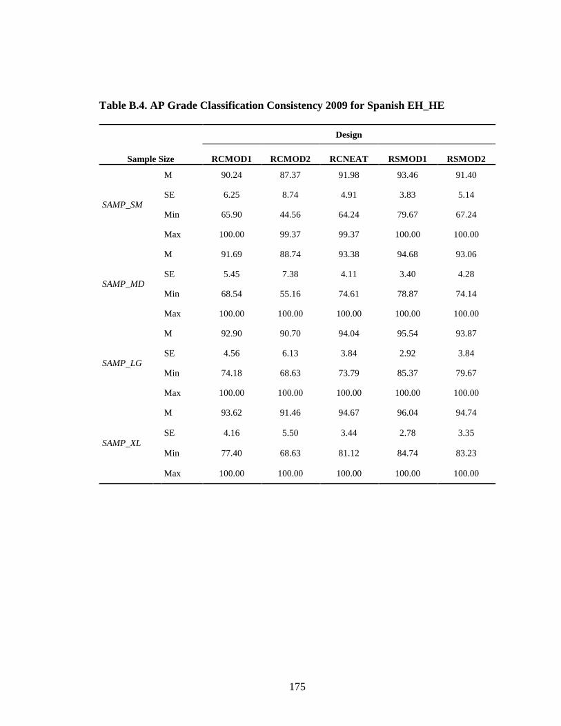
175
Table B.4. AP Grade Classification Consistency 2009 for Spanish EH_HE
Sample Size
Design
RCMOD1 RCMOD2 RCNEAT RSMOD1 RSMOD2
SAMP_SM
M 90.24 87.37 91.98 93.46 91.40
SE 6.25 8.74 4.91 3.83 5.14
Min 65.90 44.56 64.24 79.67 67.24
Max 100.00 99.37 99.37 100.00 100.00
SAMP_MD
M 91.69 88.74 93.38 94.68 93.06
SE 5.45 7.38 4.11 3.40 4.28
Min 68.54 55.16 74.61 78.87 74.14
Max 100.00 100.00 100.00 100.00 100.00
SAMP_LG
M 92.90 90.70 94.04 95.54 93.87
SE 4.56 6.13 3.84 2.92 3.84
Min 74.18 68.63 73.79 85.37 79.67
Max 100.00 100.00 100.00 100.00 100.00
SAMP_XL
M 93.62 91.46 94.67 96.04 94.74
SE 4.16 5.50 3.44 2.78 3.35
Min 77.40 68.63 81.12 84.74 83.23
Max 100.00 100.00 100.00 100.00 100.00
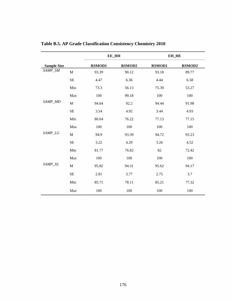
176
Table B.5. AP Grade Classification Consistency Chemistry 2010
Sample Size
EE_HH EH_HE
RSMOD1 RSMOD2 RSMOD1 RSMOD2 SAMP_SM M 93.39 90.12 93.18 89.77
SE 4.47 6.36 4.44 6.58
Min 73.3 56.13 75.39 53.27
Max 100 99.18 100 100 SAMP_MD M 94.64 92.2 94.44 91.98
SE 3.54 4.92 3.44 4.93
Min 80.04 76.22 77.13 77.15
Max 100 100 100 100 SAMP_LG M 94.9 93.39 94.72 93.23
SE 3.22 4.29 3.26 4.52
Min 81.77 76.82 82 72.42
Max 100 100 100 100 SAMP_XL M 95.82 94.31 95.62 94.17
SE 2.81 3.77 2.75 3.7
Min 85.71 78.11 85.21 77.32
Max 100 100 100 100
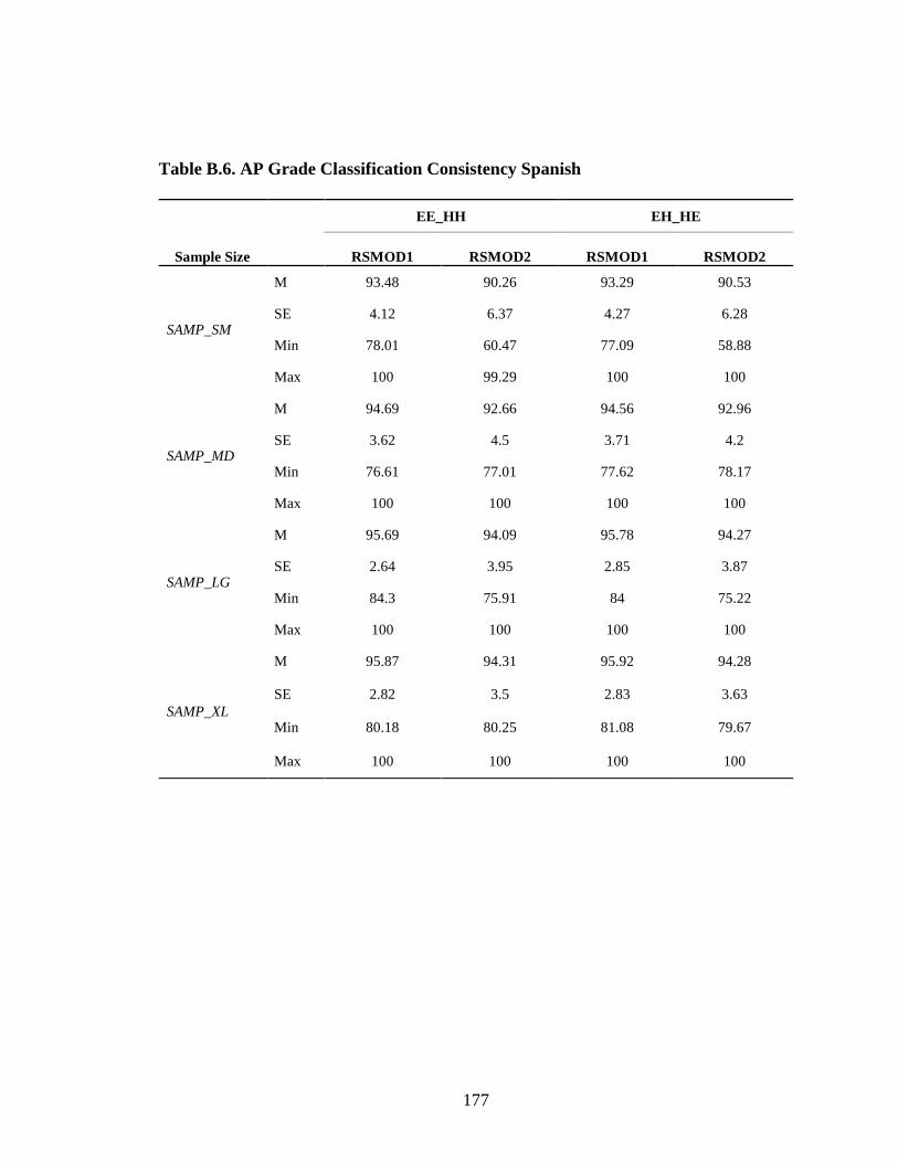
177
Table B.6. AP Grade Classification Consistency Spanish
Sample Size
EE_HH EH_HE
RSMOD1 RSMOD2 RSMOD1 RSMOD2
SAMP_SM
M 93.48 90.26 93.29 90.53
SE 4.12 6.37 4.27 6.28
Min 78.01 60.47 77.09 58.88
Max 100 99.29 100 100
SAMP_MD
M 94.69 92.66 94.56 92.96
SE 3.62 4.5 3.71 4.2
Min 76.61 77.01 77.62 78.17
Max 100 100 100 100
SAMP_LG
M 95.69 94.09 95.78 94.27
SE 2.64 3.95 2.85 3.87
Min 84.3 75.91 84 75.22
Max 100 100 100 100
SAMP_XL
M 95.87 94.31 95.92 94.28
SE 2.82 3.5 2.83 3.63
Min 80.18 80.25 81.08 79.67
Max 100 100 100 100


