Contents of talk
● Introduction to self-similar analysis● Self-similar solution with full account of charge separation● Ion energy spectrum & comparison with experiment ● Maximum ion energy● Application to Coulomb explosion
Plasma expansion into vacuum and ion accelerationproblem in terms of self-similar solution
M. MurakamiInstitute of Laser Engineering, Osaka University, Japan
Introduction to self-similar analysis
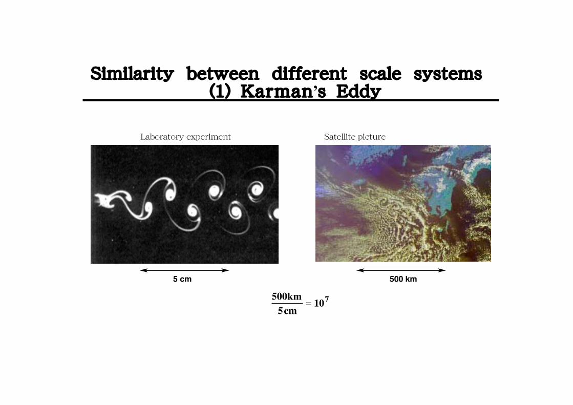
Similarity between different scale systems (1) Karman’s Eddy
500km5cm
= 107
Satellite pictureLaboratory experiment
500 km5 cm

Similarity between different scale systems (2) Blast Wave
Laboratory laser exp. Atomic explosion Nova explosion
1 cm 1 pc(3光年)100 m
100m1cm
= 104 3pc100m
= 1015
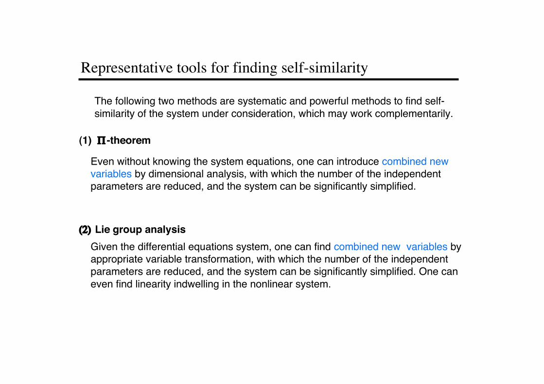
(1) Π -theorem
Even without knowing the system equations, one can introduce combined newvariables by dimensional analysis, with which the number of the independentparameters are reduced, and the system can be significantly simplified.
(2) Lie group analysisGiven the differential equations system, one can find combined new variables byappropriate variable transformation, with which the number of the independentparameters are reduced, and the system can be significantly simplified. One caneven find linearity indwelling in the nonlinear system.
Representative tools for finding self-similarity
The following two methods are systematic and powerful methods to find self-similarity of the system under consideration, which may work complementarily.

Dimensional analysis - spherical pig problem -
If a pig is assumed to be spherical,Then the only parameter is the radius.
M ∝ R3
V ∝ R 3
S ∝ R 2
Mass
Volume
Area
R≈
Try to simplify the system as much as possible, but be careful not to loose the essence.
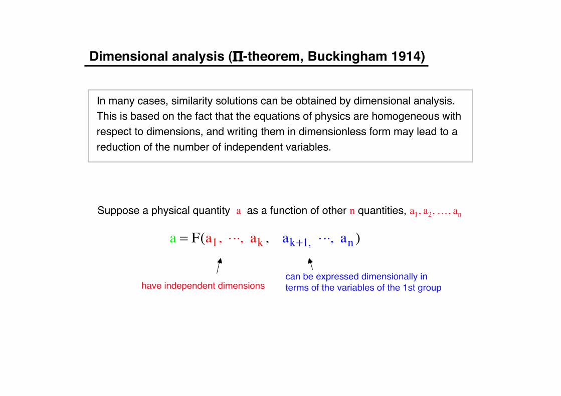
Dimensional analysis (Π-theorem, Buckingham 1914)
In many cases, similarity solutions can be obtained by dimensional analysis.This is based on the fact that the equations of physics are homogeneous withrespect to dimensions, and writing them in dimensionless form may lead to areduction of the number of independent variables.
Suppose a physical quantity a as a function of other n quantities, a1, a2, …, an
have independent dimensionscan be expressed dimensionally in terms of the variables of the 1st group
a = F(a1, ⋅ ⋅⋅, ak , ak+1, ⋅ ⋅⋅, an )
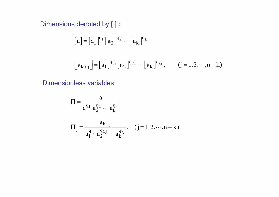
a[ ] = a1[ ]q1 a2[ ]q2 ⋅ ⋅ ⋅ ak[ ]qkDimensions denoted by [ ] :
Dimensionless variables:
Π = aa1q1 a2
q2 ⋅ ⋅ ⋅akqk
Π j =ak+ j
a1q1j a2
q2 j ⋅ ⋅ ⋅akqkj, ( j= 1,2,⋅ ⋅ ⋅,n − k)
ak+ j⎡⎣ ⎤⎦ = a1[ ]q1j a2[ ]q2 j ⋅ ⋅ ⋅ ak[ ]qkj , ( j= 1,2,⋅ ⋅ ⋅, n − k)

Substitution for and for :a ak+ j
Here the right-hand-side must not depend onwith independent dimensions, because the left-hand-sidedoes not. Otherwise, invariance with respect to system ofunits would be violated. Therefore:
Π =F a1,⋅ ⋅ ⋅,ak , Π1a1
q11 ⋅ ⋅ ⋅akqk1 ,⋅ ⋅ ⋅,Πn+ka1
q1,n+k ⋅ ⋅ ⋅akqk,n+k( )
a1q1 ⋅ ⋅ ⋅ak
qk
Π Π j
Π = Φ(Π1,Π2,⋅ ⋅ ⋅,Πn−k ) (Π-theorem)
⇒ for k = n −1, Π = Φ(Π1) similarity solution⇒ for k = n, Π = Φ0

A typical example of Π-theorem
(cm) : (sec) :
(g/cm3) :
(erg) :
ρ0[ ] = ML−3
E[ ] = ML2T−2
r[ ] = Lt[ ] = T
The number of dimensions of the system:T, M, L ( k = 3)
The number of nondimensional parameters :
Π-Theorem
The number of parameters that characterize the system: n = 4
RadiusTimeDensityEnergy
n − k = 1
Π1 =ρ0E
⎛⎝⎜
⎞⎠⎟1/5 rt2/5
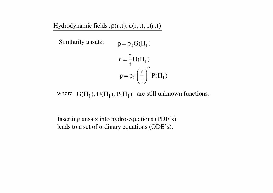
Hydrodynamic fields :ρ(r, t), u(r, t), p(r, t)
ρ = ρ0G(Π1)
u = rtU(Π1)
p = ρ0rt
⎛⎝⎜
⎞⎠⎟2P(Π1)
Similarity ansatz:
Inserting ansatz into hydro-equations (PDE’s)leads to a set of ordinary equations (ODE’s).
where G(Π1), U(Π1), P(Π1) are still unknown functions.

Taylor-Sedov (-Von Neumann) Blast Wave
rf (m)
t (sec)

Lie Group Analysis - symmetry of differential equations -
Marius Sophus LieNorwegian mathematicianEnd of 19th century
Discovery of the symmetry
Introduction of a new combined variable
Partial differential system Ordinary differential system
Higher order system Lower order system
Nonlinear system Linear system
⇩
Finding of self-similar solution
⇩
⇩
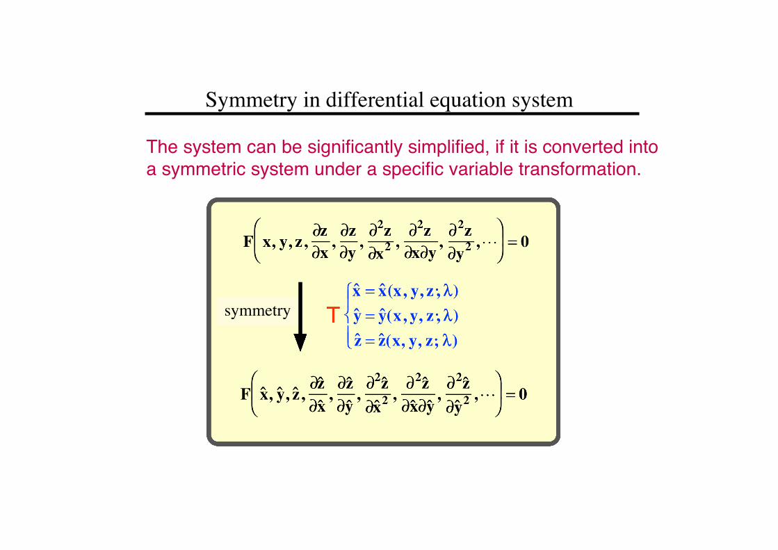
Symmetry in differential equation system
The system can be significantly simplified, if it is converted intoa symmetric system under a specific variable transformation.
symmetry
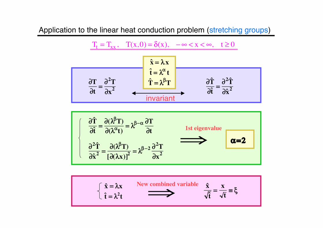
Application to the linear heat conduction problem (stretching groups)
∂T∂t
=∂2T∂x2
∂ ˆ T ∂ˆ t
=∂2 ˆ T ∂ˆ x 2
ˆ x = λxˆ t = λα tˆ T = λβT
invariant
∂ ˆ T ∂ˆ t
=∂(λβT)∂(λαt)
= λβ−α∂T∂t
∂2 ˆ T ∂ˆ x 2
=∂(λβT)
[∂(λx)]2= λβ−2 ∂2T
∂x2
⇒1st eigenvalue
α = 2
⇒ˆ x = λxˆ t = λ2t
New combined variable ˆ x ˆ t =
xt≡ ξ
Tt = Txx, T(x,0) = δ(x), −∞ < x < ∞, t ≥ 0
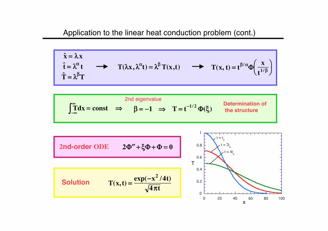
Application to the linear heat conduction problem (cont.)
0
0.2
0.4
0.6
0.8
1
0 20 40 60 80 100x
T
t = t0
t = 4t0
t = 2t0
ˆ x = λxˆ t = λα tˆ T = λβT
T(λx, λαt) = λβT(x,t) T(x, t) = tβ /αΦ x
t1/β⎛ ⎝
⎞ ⎠
β = −1 ⇒ T = t−1/ 2Φ(ξ)Determination of the structure⇒Tdx =
−∞
∞
∫ const
2 ′ ′ Φ + ξΦ + Φ = 02nd-order ODE
T(x, t) = exp(−x2 /4t)
4πtSolution
2nd eigenvalue
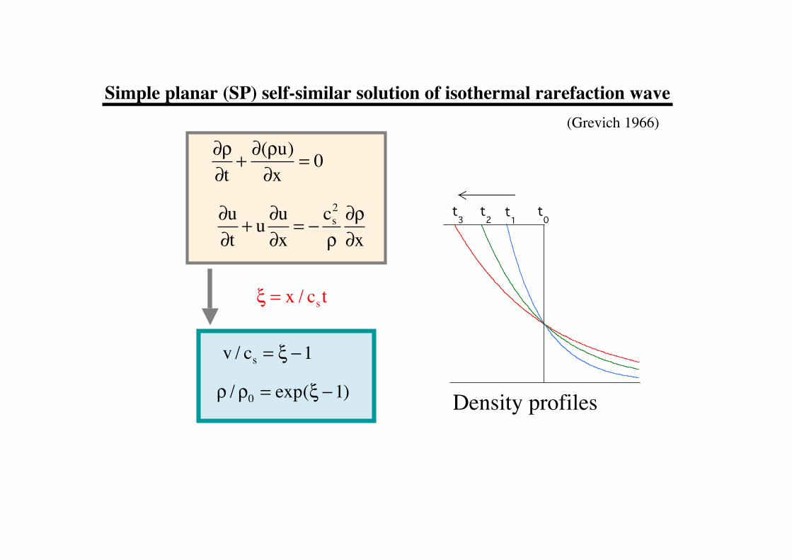
Simple planar (SP) self-similar solution of isothermal rarefaction wave
t0
t3t2t1
∂ρ∂t
+ ∂(ρu)∂x
= 0
∂u∂t
+ u ∂u∂x
= − cs2
ρ∂ρ∂x
ξ = x / cst
v / cs = ξ −1
Density profilesρ /ρ0 = exp(ξ −1)
(Grevich 1966)

Comparison between the present model and the semi-infinite model
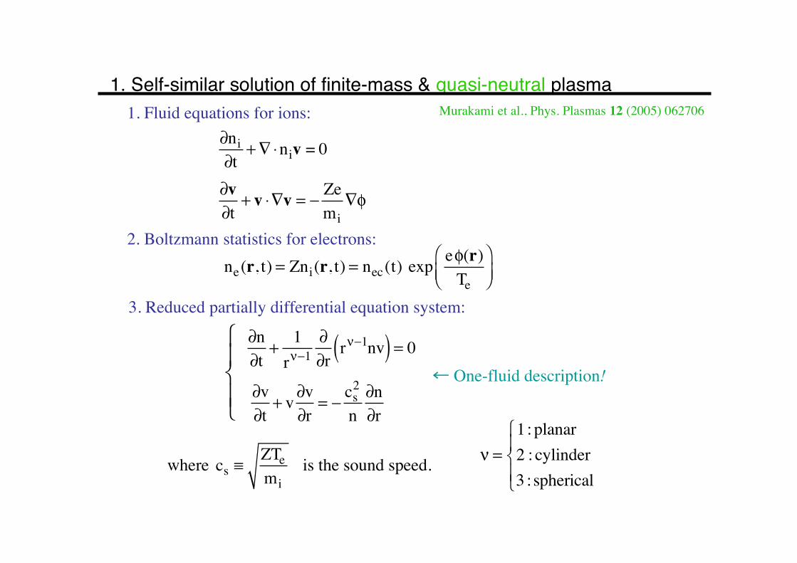
1. Self-similar solution of finite-mass & quasi-neutral plasma
∂ni∂t
+∇⋅niv = 0
∂v∂t
+ v ⋅∇v = − Zemi
∇φ
ne(r, t) = Zni(r, t) = nec(t) expeφ(r)Te
⎛⎝⎜
⎞⎠⎟
cs ≡ZTemi
1. Fluid equations for ions:
2. Boltzmann statistics for electrons:
∂v∂t
+ v ∂v∂r
= − cs2
n∂n∂r
3. Reduced partially differential equation system:
where is the sound speed.
⎧⎨⎪
⎩⎪← One-fluid description!
ν =1:planar2 : cylinder3 :spherical
⎧⎨⎪
⎩⎪
∂n∂t
+ 1rν−1
∂∂rrν−1nv( ) = 0
Murakami et al., Phys. Plasmas 12 (2005) 062706
Self-similar solution of finite-mass & quasi-neutral plasma (cont’d)
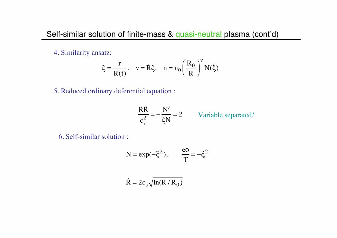
4. Similarity ansatz:
ξ = r
R(t), v = Rξ, n = n0
R0R
⎛⎝⎜
⎞⎠⎟νN(ξ)
5. Reduced ordinary deferential equation :
RRcs2 = − ′N
ξN= 2 Variable separated!
6. Self-similar solution :
N = exp(−ξ2 ), eφT
= −ξ2
R = 2cs ln(R / R0 )
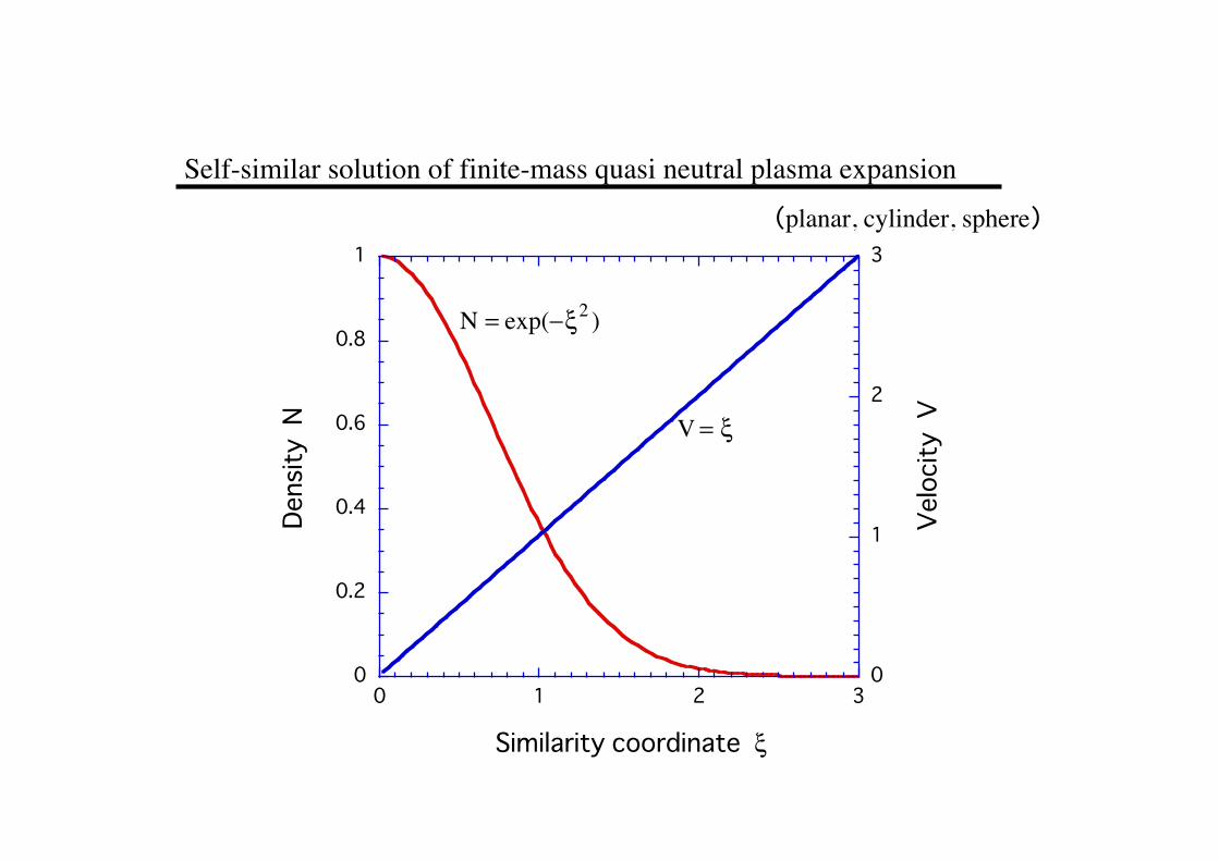
Self-similar solution of finite-mass quasi neutral plasma expansion
0
0.2
0.4
0.6
0.8
1
0
1
2
3
0 1 2 3
Density N
Velocity V
Similarity coordinate ξ
N = exp(−ξ2 )
V = ξ
(planar, cylinder, sphere)

100
101
102
103
104
105
106
10-1 100 101 102 103 104 105
ν = 1, 2, 3: 等温膨張 R(t)
R(t)/R0
cst/R0
Temporal evolution of the system characteristic scale
R ∝ t
Isothermal case

(a) Finite mass
(1) Isothermal expansion
(3) others (a) Maxwellian
Ion energy spectra obtained from quasi-neutral model
dNdε
∝ ε(ν−2)/2 exp(−ε) =exp(−ε) ε (ν = 1)exp(−ε) (ν = 2)exp(−ε) ε (ν = 3)
⎧
⎨⎪
⎩⎪
(a) Finite mass
(b)half-infinitely- stretched plane
dNdε
∝ exp(− ε ) ε
(2) Adiabatic expansion(planar/initially isentropic distribution)
PlaneCylinderSphere
dNdε
∝ 1− γ −12( ε −1)⎛
⎝⎜⎞⎠⎟2/(γ −1)
ε
dNdε
∝ (1− ε)1/(γ −1) ε
dNdε
∝ exp(−ε) ε
(b)half-infinitely- stretched plane

The analytical model excellently reproduces the experimental results on ion kinetic energy spectrum (planar geometry)
10-6
10-5
10-4
10-3
10-2
10-1
100
0.1 1 10Ion kinetic energy ε (keV)
Experiment
(α =1, ε0=1.7 keV)
Norm
alize
d sp
ectru
m d
N/dε
Present model
1Maximum ion energy predicted by the present analytical model
Murakami et al., Phys. Plasmas 12 (2005) 062706
Sn solid plane
Laser

The analytical model excellently reproduces the experimental results on ion kinetic energy spectrum (spherical geometry)
Murakami et al., Phys. Plasmas 12 (2005) 062706
10-4
10-3
10-2
10-1
100
0.1 1 10
Normalized spectrum dN/d
ε
Ion kinetic energy ε (keV)
Experiment
Present model
1
(α =3, ε0= 3.0 keV)
Maximum ion energy predicted by the present analytical model
Xe liquid jet
Laser
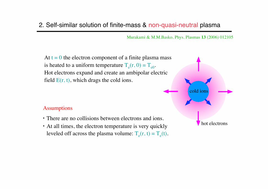
hot electrons
cold ions
At t = 0 the electron component of a finite plasma massis heated to a uniform temperature Te(r, 0) = Te0.Hot electrons expand and create an ambipolar electricfield E(r, t), which drags the cold ions.
・There are no collisions between electrons and ions.・At all times, the electron temperature is very quickly leveled off across the plasma volume: Te(r, t) = Te(t).
Assumptions
2. Self-similar solution of finite-mass & non-quasi-neutral plasmaMurakami & M.M.Basko, Phys. Plasmas 13 (2006) 012105
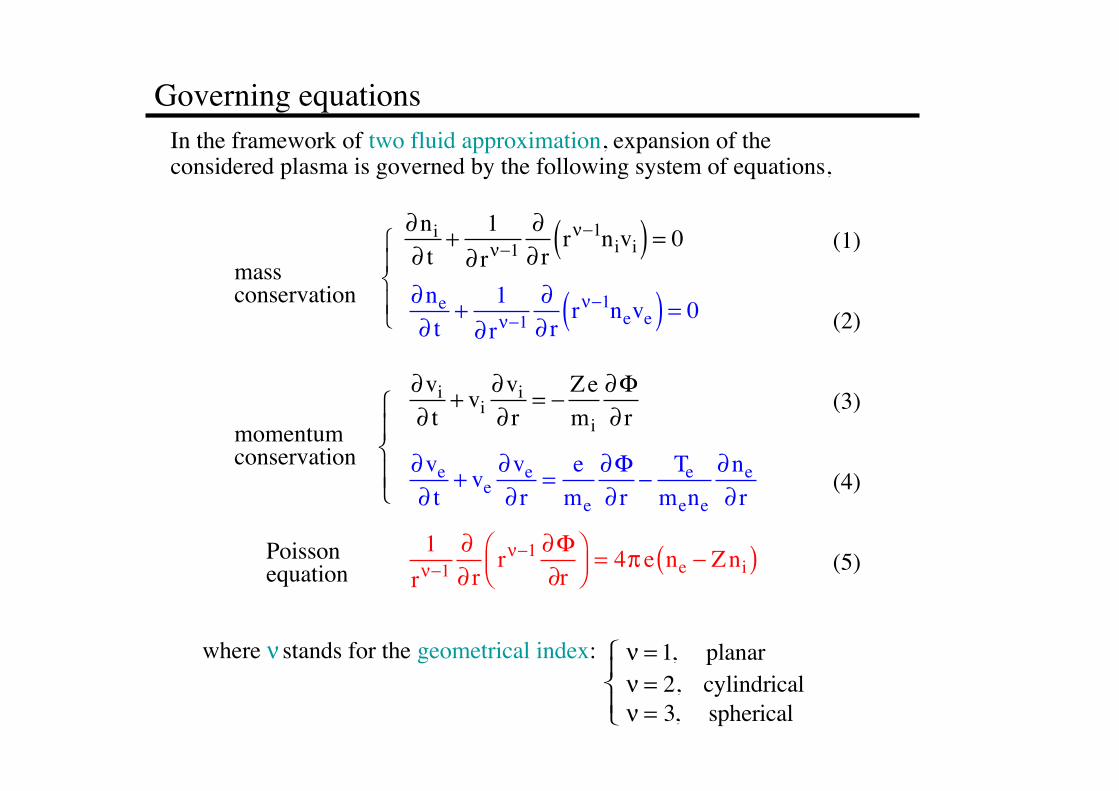
Governing equations
where ν stands for the geometrical index: ν = 1, planarν = 2, cylindricalν = 3, spherical
⎧⎨⎪
⎩⎪
In the framework of two fluid approximation, expansion of theconsidered plasma is governed by the following system of equations,
∂ni∂ t
+ 1∂ rν−1
∂∂ r
rν−1nivi( ) = 0∂ne∂ t
+ 1∂ rν−1
∂∂ r
rν−1neve( ) = 0⎧⎨⎪
⎩⎪massconservation
∂vi∂ t
+ vi∂vi∂ r
= − Zemi
∂Φ∂ r
∂ve∂ t
+ ve∂ve∂ r
= eme
∂Φ∂ r
− Temene
∂ne∂ r
⎧⎨⎪
⎩⎪
momentumconservation
1rν−1
∂∂ r
rν−1 ∂Φ∂r
⎛⎝⎜
⎞⎠⎟ = 4π e ne − Zni( )Poisson
equation
(1)
(2)
(3)
(4)
(5)

Similarity ansatzThe key assumption is that the velocity, v(r, t), is linear in radius. This isalways correct for the asymptotic stage of free expansion of a finite mass.
ve(r, t) = vi(r, t) = Rξ
ξ = r
R(t), R ≡ dR
dt
ne(r, t) = ne0R0R(t)
⎛⎝⎜
⎞⎠⎟ν
Ne(ξ), Ne(0) = 1
Zni(r, t) = ni0R0R(t)
⎛⎝⎜
⎞⎠⎟ν
Ni(ξ), Ni(0) ≠ 1
(6)
(7)
(8)
(9)
NiNe
ξf
Cold ions preserve a sharp edge at ξ = ξf(still unknown).
Functions, vi and Ni, are then definedonly for 0 ≤ ξ ≤ ξf
●
●
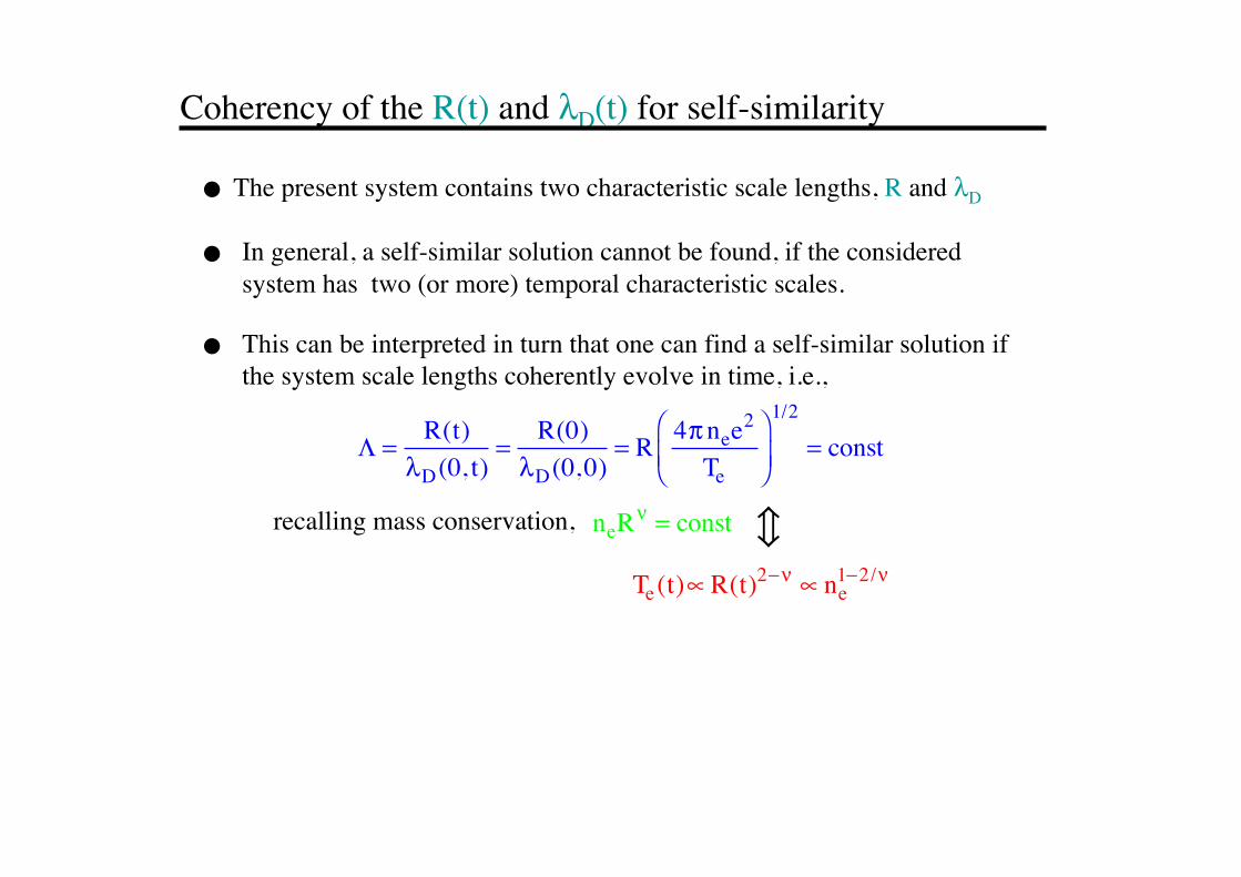
Coherency of the R(t) and λD(t) for self-similarity
The present system contains two characteristic scale lengths, R and λD
In general, a self-similar solution cannot be found, if the consideredsystem has two (or more) temporal characteristic scales.
●
●
This can be interpreted in turn that one can find a self-similar solution ifthe system scale lengths coherently evolve in time, i.e.,
●
Λ = R(t)λD(0, t)
= R(0)λD(0,0)
= R 4πnee2
Te
⎛
⎝⎜⎞
⎠⎟
1/2
= const
neRν = constrecalling mass conservation,
Te(t)∝R(t)2−ν ∝ ne
1−2/ν
Self-similar solution
Continuity equations (1) and (2) are automatically satisfied for any R(t), Ne(ξ) and Ni(ξ). The electron equation of motion (4) yields
This is the well-known Boltzmann relation generalized to the case of .
Ne = exp(φ − µeξ2 )
µe > 0
The ion equation of motion (3) yields
for 0 < ξ < ∞
φ(ξ) = −ξ2 for ξ < ξfSpatial profile
Temporal evolution
R(t) =
2cs02 t / R0, ν = 1
2cs0 ln R(t) / R0( ), ν = 22cs0 1−R0 / R(t), ν = 3
⎧
⎨⎪⎪
⎩⎪⎪
cs0 =ZTe0mi
⎛
⎝⎜⎞
⎠⎟
whereφ = eΦ / Te
µe = Zme /mi
⎧⎨⎩
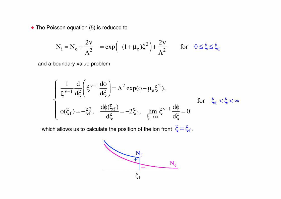
The Poisson equation (5) is reduced to
Ni = Ne +2νΛ2
= exp −(1+ µe )ξ2( ) + 2ν
Λ2for 0 ≤ ξ ≤ ξf
and a boundary-value problem
1ξν−1
ddξ
ξν−1 dφdξ
⎛⎝⎜
⎞⎠⎟= Λ2 exp(φ − µeξ
2 ),
φ(ξf ) = −ξf2 , dφ(ξf )
dξ= −2ξf , lim
ξ→∞ξν−1 dφ
dξ= 0
which allows us to calculate the position of the ion front
for ξf < ξ < ∞
⎧⎨⎪
⎩⎪
ξ = ξf .
NiNe
ξf

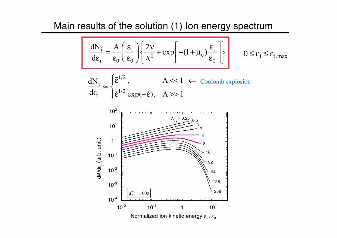
Main results of the solution (1) Ion energy spectrum
dNi
dεi= Aε0
εi
ε0
⎛⎝⎜
⎞⎠⎟2νΛ2
+ exp −(1+ µe )εi
ε0
⎡
⎣⎢
⎤
⎦⎥
⎧⎨⎩
⎫⎬⎭
dNi
dεi∝ε1/2 , Λ <<1ε1/2 exp(− ε), Λ >>1
⎧⎨⎪
⎩⎪
Coulomb explosion⇐
10-4
10-3
10-2
10-1
100
101
102
10-2 10-1 100 101
0.5Λss
= 0.251
24
8
16
32
64
128
256
d Ni/dε i (
arb.
uni
t)
1
1
Normalized ion kinetic energy ε i / ε0
µe−1 = 1000
0 ≤ εi ≤ εi,max
ξf2 =
W π1/3Λ4/3 / 2µe( ) / 2, Λ <<1
W(Λ2 / 2), Λ >>1
⎧⎨⎪
⎩⎪
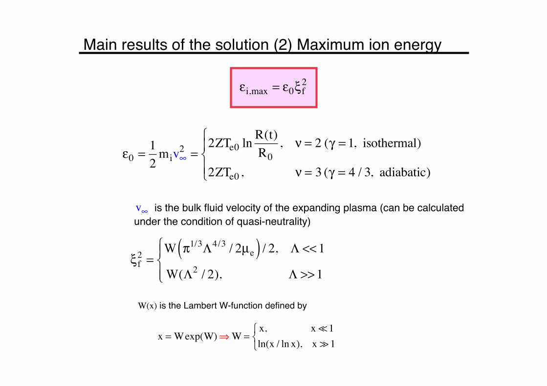
Main results of the solution (2) Maximum ion energy
εi,max = ε0ξf2
is the bulk fluid velocity of the expanding plasma (can be calculatedunder the condition of quasi-neutrality)v∞
ε0 =12miv∞
2 =2ZTe0 ln
R(t)R0
, ν = 2 (γ = 1, isothermal)
2ZTe0 , ν = 3 (γ = 4 / 3, adiabatic)
⎧⎨⎪
⎩⎪
W(x) is the Lambert W-function defined by
x =Wexp(W)⇒W =
x, x1ln(x / ln x), x1
⎧⎨⎩
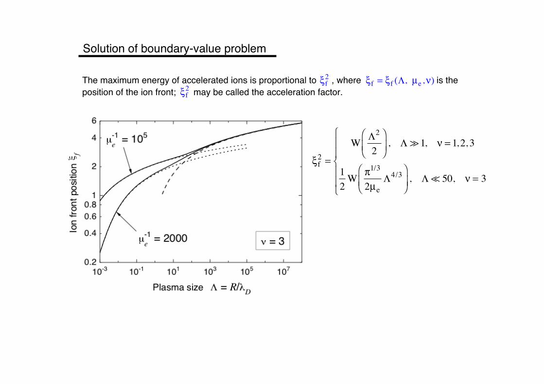
ξf2 =
W Λ2
2⎛
⎝⎜⎞
⎠⎟, Λ1, ν = 1,2, 3
12W π1/3
2µeΛ4/3
⎛
⎝⎜⎞
⎠⎟, Λ 50, ν = 3
⎧
⎨
⎪⎪
⎩
⎪⎪
The maximum energy of accelerated ions is proportional to , where is theposition of the ion front; may be called the acceleration factor.
ξf2 ξf = ξf (Λ, µe ,ν)
ξf2
Solution of boundary-value problem

Generalization of the main resultWe believe our result for to be more general than the self-similar solution itself. εi,max
Poisson equation:
Boltzmann distibution:
Energy balance:Zni
ne
+
−
∂2φ∂x2
= 4πene
ne = ne0 expeφTe
⎛⎝⎜
⎞⎠⎟
⎫
⎬⎪⎪
⎭⎪⎪
⇒ ∂2φ∂x2
= 4πene0 expeφT
⎛⎝⎜
⎞⎠⎟
Argument: For µe<<1 and Λ>>1 one can integrate the Poisson equation over the electronsheath to obtain the electric field at the ion front and the maximum ion energy:
12Ef2 = 4πnefTe
Ef = 8πnefTe ∝ nef ∝ ref−γν/2 εi,max = Ze Efdrf
rf 0
∞
∫ ∝ rf−γν/2drf
rf 0
∞
∫⇒
The integral converges whenever γ ν > 2, which means that all the acceleration occursDuring the initial phase of expansion.

Time
等温膨張領域
Isothermal Expansion
断熱膨張領域
Adiabatic Expansion
Laser On
エネルギースペクトル
の構造はここで決まる!
Laser Off
エネルギースペクトル
の構造は殆ど変化しない
εi,max ≈ ε0W(Λ02 / 2)
where ε0 =12miv∞
2 =2ZTe0 ln
R(t)R0
, γ = 1 (isothermal)
2ZTe0 / ν(γ −1), γ >1 (adiabatic)
⎧⎨⎪
⎩⎪
where is measured at the onset of the asymptotic phase of expansion.
Λ0 = Λ(t0 )
Te0
Te(t)
Time t
ne(t, 0)
t0
Generalized form of the maximum ion energyFor any , the maximum ion energy in cylindrically and sphericallyexpanding plasmas is given by
γ ≥1

• Self-similar solution exists only in the framework ofthe quasi-neutral hydrodynamics.
P.Mora (PRL, 2003) obtained an accurate numericalsolution for µe = 0.
In the limit of the ions at the front are acceleratedto the infinite energy.
•
•
εi,max = 2ZTe0 ln cstλD
⎛⎝⎜
⎞⎠⎟
2
= 2ZTe0 lncstλD
⋅ ln cstλD
12mivbulk
2⇓
The simple planar solution is the plane-parallel isothermal expansion of a plasma, initially occupying a half-space.
Comparison with the SP solution (P. Mora, 2003)
t→∞
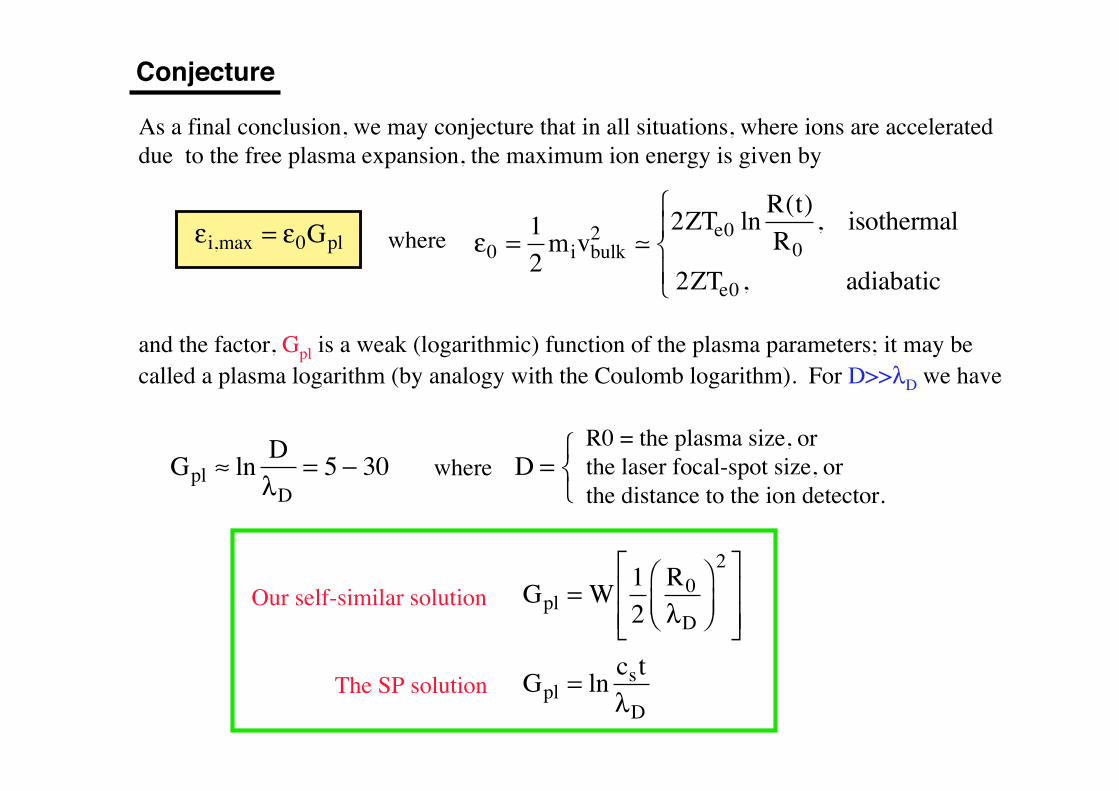
Conjecture
As a final conclusion, we may conjecture that in all situations, where ions are accelerated due to the free plasma expansion, the maximum ion energy is given by
εi,max = ε0Gpl where
and the factor, Gpl is a weak (logarithmic) function of the plasma parameters; it may becalled a plasma logarithm (by analogy with the Coulomb logarithm). For D>>λD we have
Gpl ≈ lnDλD
= 5 − 30 whereR0 = the plasma size, or the laser focal-spot size, orthe distance to the ion detector.
D =⎧⎨⎩
Our self-similar solution Gpl =W12R0λD
⎛⎝⎜
⎞⎠⎟
2⎡
⎣⎢⎢
⎤
⎦⎥⎥
The SP solution Gpl = lncstλD
ε0 =12mivbulk
2 2ZTe0 ln
R(t)R0
, isothermal
2ZTe0 , adiabatic
⎧⎨⎪
⎩⎪
Application to Coulomb explosion

10-4
10-3
10-2
10-1
100
101
0
2
4
6
8
10
0 1 2 3 4 5 6
Norm
alize
d de
nsiti
es N
e, Ni
Elec
tric
field
E
Self-similar coordinate ξ
Ni
Ne
E
1 µe−1 = 2000
ν = 3 Λss = 2
The self-similar solution can described plasma expansions of any size
Λ ~ 1 Λ ~ 106

0
0.2
0.4
0.6
0.8
1
1.2
0.1 1 10 100
Ener
gy tr
ansf
er ra
tio η
tra
Initial plasma size Λuni
Simulation
Theory
4.5
450
1400
4.5
45
450
4500Te0 = 4500eV
Rf0 = 10nm
Rf0 = 2.2 nm
ne0 = 1021cm−3
ne0 = 1023cm−3
45
(µe−1 = 100)
µe−1 = 100
µe−1 = 1000
Energy transfer efficiency from electrons to ions
Summary
• A new self-similar solution is found to describe the plasma expansion intovacuum with full account of the charge separation.
• The experimental results have turned out to be excellently reproduced by thepresent solution.
• The maximum ion energy has been also obtained in a simple analytical form,for example for spherical geometry, εi,max = 2ZTe0 ln(Λ
2 / 2)
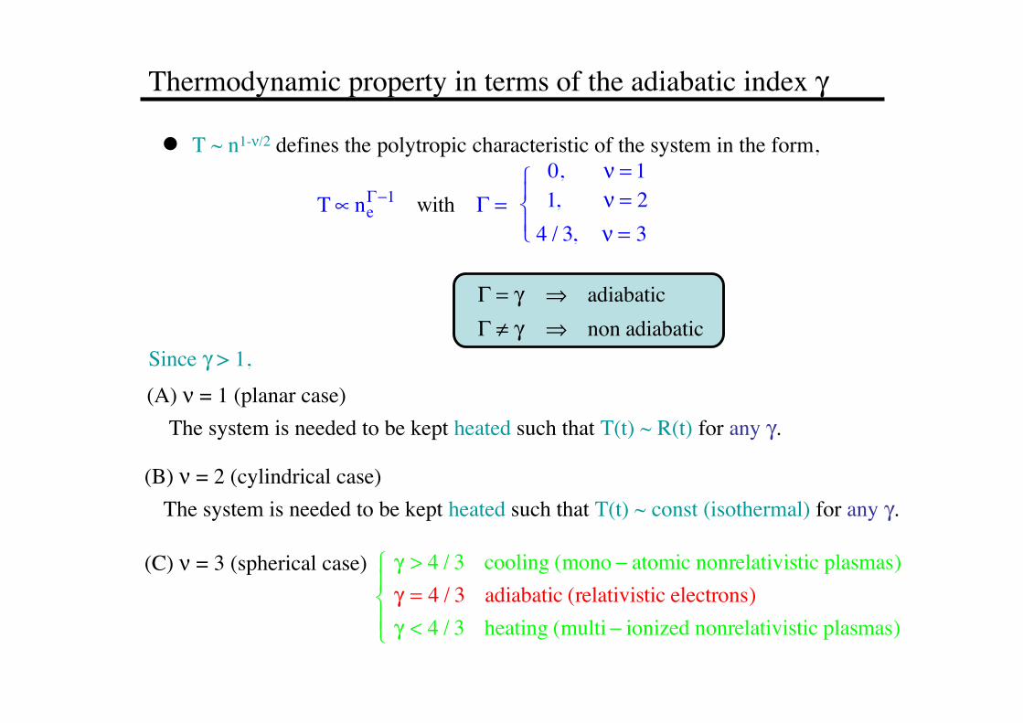
Thermodynamic property in terms of the adiabatic index γ
T ~ n1-ν/2 defines the polytropic characteristic of the system in the form,●
T∝ neΓ−1 with Γ =
⎧⎨⎪
⎩⎪
0, ν = 1
4 / 3, ν = 31, ν = 2
Γ = γ ⇒ adiabaticΓ ≠ γ ⇒ non adiabatic
(A) ν = 1 (planar case)The system is needed to be kept heated such that T(t) ~ R(t) for any γ.
(B) ν = 2 (cylindrical case)The system is needed to be kept heated such that T(t) ~ const (isothermal) for any γ.
(C) ν = 3 (spherical case)
Since γ > 1,
⎧⎨⎪
⎩⎪
γ > 4 / 3 cooling (mono − atomic nonrelativistic plasmas)γ = 4 / 3 adiabatic (relativistic electrons)γ < 4 / 3 heating (multi− ionized nonrelativistic plasmas)


