
The government budget constraint and the scope for fiscal policy
École des Hautes Études Commerciales (HÉC)January 2001

The public sector accounts
The primary balance and the debt service
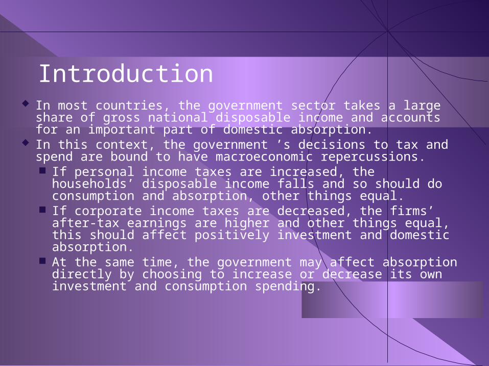
Introduction In most countries, the government sector takes a large share of
gross national disposable income and accounts for an important part of domestic absorption.
In this context, the government ’s decisions to tax and spend are bound to have macroeconomic repercussions. If personal income taxes are increased, the households’
disposable income falls and so should do consumption and absorption, other things equal.
If corporate income taxes are decreased, the firms’ after-tax earnings are higher and other things equal, this should affect positively investment and domestic absorption.
At the same time, the government may affect absorption directly by choosing to increase or decrease its own investment and consumption spending.

The government’s budget balance Before examining the macroeconomic repercussions of
these decisions, it is useful to look at the basics of government budget accounting.
The government ’s overall budgetary balance (BB) is equal to the difference between total revenues (TR) and total expenditures (TE): BB = TR - TE
However, the government has little (if any) control over the debt service in the short-run. This is why we usually distinguish between program spending (PS) and debt service (DS): BB = (TR - PS) - DS
The difference between total revenues and program spending (TR-BS) is called the primary balance (PB), so we write: BB = PB -DS

The main items of the government budget
Total revenues (R) Tax revenue
> Direct taxes (household and corporate income taxes)
> Indirect taxes (VAT, import taxes, etc.)
Other revenue
> Dividends paid by the state-owned enterprises
> Investment income (ex.: interest on the foreign reserve assets)
Total expenditures (TE)
Program Spending (PS)
> Goods and services (G
and IG)
> Transfers and subsidies
Debt service (DS)
> Interest paid to the
holders of government
debt (treasury bills,
bonds and other
government debt
instruments)

Surpluses and deficits Interpretation:
The government budgetary balance would be equal to the primary balance if the government had no debt.
The government budgetary balance is positive (and there is a budget surplus)
when the primary balance is positive and higher than the debt service (PB DS).
The government budgetary balance is negative (and there is a budget deficit)
when the primary balance is negative or when the primary balance is positive but smaller than the
debt service (PB DS).
A primer on fiscal policy
Keynesian fiscal policy

A primer on fiscal policy
In the short-run, only the primary balance can be affected by government decisions.
In principle, the primary balance could be an intermediate target by which the government aims to influence aggregate demand and the macroeconomic equilibrium of the economy (final target).
The instruments would be government spending and taxes: If the government wants to stimulate aggregate
demand, it may reduce taxes and/or increase spending (G and IG).
PB deteriorates and AD is higher, other things equal. If the government wants to slow aggregate demand, it
may increase taxes and/or decrease spending (G and IG).
PB improves and AD is lower, other things equal

AD(PB down)
P+
Y+
AD0
P
AD = AS = Y
AS
Y0
P0
AD(PB up)
Y-
P-

A primer on fiscal policy
The idea that we might use the primary balance as an intermediate target for macroeconomic stabilization is at the heart of what is called keynesian fiscal policy.
The keynesian idea was that the government should be prepared to run a primary deficit in times of recession and should revert to a primary surplus in better times.
This way, the primary balance would be zero on average and there would be no growth in the public debt over the economic cycle.
The problem has been that many governments have for too long applied only the first half of the keynesian recipe and their debt has grown at an unsustainable pace.

Keynesian fiscal policy
Primary surplus
Primary deficit
Booming times
Recessive times
0

Irresponsible fiscal policy
Primary surplus
Primary deficit
Booming times
Recessive times
0

The government budget constraint
What is sustainable and what is not

The government budget constraint When PB < DS, the government budgetary balance is
negative, there is a budget deficit and this deficit must be financed somehow.
Aside from monetary financing (we’ll see that later), there are three basic sources of government deficit financing: The government may borrow from the domestic
residents and its domestic debt will increase (D > 0) The government may borrow from the foreign residents
and its foreign debt will increase (D* > 0) The government may sell its assets.
Deficit = D + D* - Assets

The government budget constraintLet ’s define the total net debt (D + D* - Assets) as B. Since the budget deficit is equal to DS - PB, we can write:
B = DS - PB Suppose there is a constant average interest rate i on the
net public debt. Then the debt service DS will be equal to i B and we write:
B = i B - PB ,which in discrete time can be written as Bt - B t-1 = i B t-1 - PBt ,or Bt = (1+ i ) B t-1 - PBt

The government budget constraint However, the size of the debt B tells us very little unless
we know the size of the economy. Since the debt is in nominal terms, we have to compare it
to nominal GDP (YN). Let ’s define B/YN as b, PB/YN as pb and the growth rate of nominal GDP as ng. Then we have:
YNt
bt = (1+ i ) B t-1 - pbt
(1+ng)
bt = (1+ i ) b t-1 - pbt
Which can be simplified to

The government budget constraint We could (but will not) show that this relationship is also
true in real terms (using r instead of i and rg - the growth rate of real GDP - instead of gn:
(1 + rg)
bt = (1+ r ) b t-1 - pbt
Conclusion: When the real rate of interest is higher than the real growth rate of the economy, the debt to GDP ratio grows exponentially unless the government runs a sufficiently high primary balance surplus.

An exemple of explosive debt dynamics
Canadian public finances in the middle of the 1990 ’s

At the beginning of the 1990 ’s
The government ’s financial situation was rapidly
deteriorating.
The deficit and the public debt were rising to an extent
such that raised the question of the government ’s financial
credibility.
The government ’s budgetary balance had become
extremely vulnerable to a rise in the level of interest rates.
Financial markets were getting nervous.
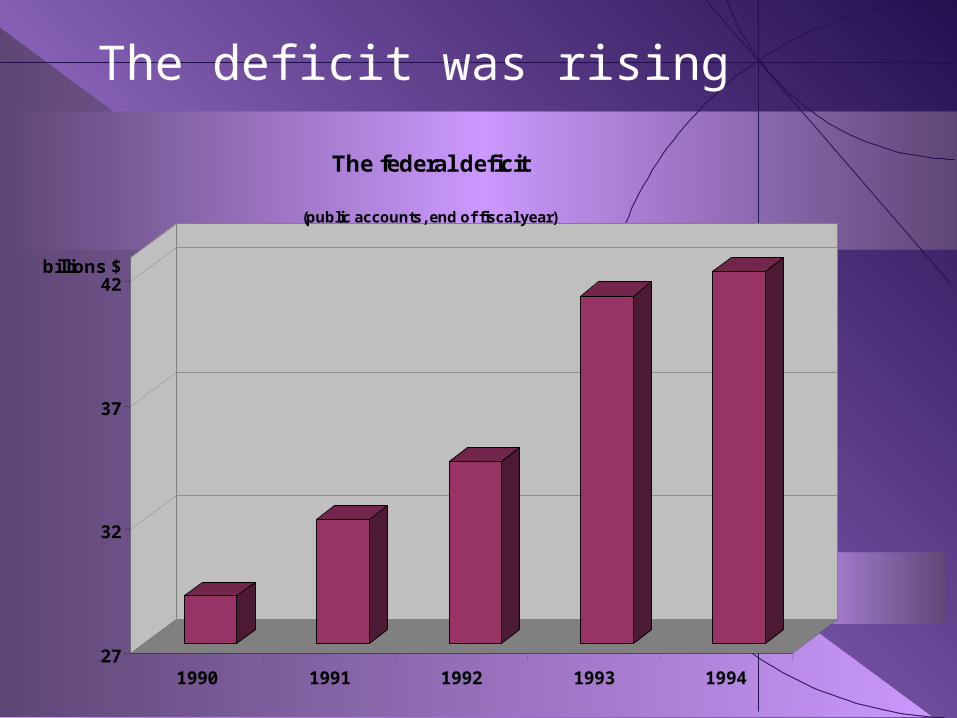
The deficit was rising
27
32
37
42billions $
1990 1991 1992 1993 1994
The federal deficit
(public accounts, end of fiscal year)

The net public debt was exploding
35
40
45
50
55
60
65
70% of GDP
1988 1989 1990 1991 1992 1993 1994 1995Year
Public administrations net debt(national accounts)
Canada USA

Debt service(% of tax revenues)
65%
36%Debt service
Program spending
Debt service was taking a large share of total tax revenues leaving little to program spending

The origin of the problem
For two decades, the government ’s net debt (ND) had increased more rapidly than nominal GDP, that is, more rapidly than the government ’s tax base.
Consequently, debt service had come to take a large share of total tax revenues.
The situation was clearly unsustainable in the long run (debt service cannot absorb 100 % of total tax revenues - nothing would then be left for program spending -) but in the meanwhile, the government was keeping on borrowing.
The goodwill of financial markets had become critical but this had some limits.

Public debt and interest rates
The analytical model

1/r
Nominal value
D = Demand
Supply = B = outstanding stock of government bonds
1/r0
r = rate of return on government bonds

1/r
Nominal value
D = f (Sp, ra, a, )
Supply = B = Public debt
With BB <0With BB>0
1/r0
Note: Sp = private savings (depends on GDP), ra = expected rate of return on alternative assets, a= expected rate of inflation (depends on monetary policy and other things), = other factors , r = rate of return.

Nominal value
1/r0
1/r
D
B
1/r1
B’
Other things equal, an increase in the stock of government bonds (from B to B’)cause an increase in their rate of return (1/r falls)

1/r
Nominal value
D
B
1/r0
1/r1
B’
Other things equal, a fall in the stock of government bonds (from B to B’) reduces their rate of return (1/r increases).

In normal times, nominal GDP grows every year
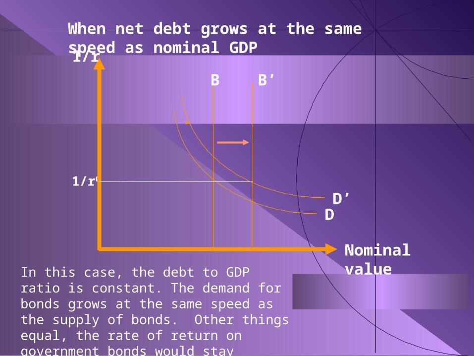
If nominal GDP grows at the same speed as net debt
(e.g. growth rates are the same), the debt to GDP
ratio is constant.
If nominal GDP grows at a higher speed than net
debt, the debt to GDP ratio declines.
If nominal GDP grows at a lower speed than net debt,
the debt to GDP ratio increases.

The growth in nominal GDP feeds into a higher demand for government bonds
When nominal GDP grows, so do aggregate
revenues and savings.
For a constant saving rate, savings and GDP
would grow at the same percentage rate.
With an increase in savings, the demand for all
financial assets is stimulated.
If there are no change in the way people diversify
their portfolio between bonds, stocks and other
assets, the demand for government bonds should
grow at the same speed as savings and thus at
the same speed as GDP.
Nominal value
1/r0
1/r
D
B
In this case, the debt to GDP ratio is constant. The demand for bonds grows at the same speed as the supply of bonds. Other things equal, the rate of return on government bonds would stay constant.
When net debt grows at the same speed as nominal GDP
B’
D’

Nominal value
1/r0
1/r
D
B
What about if net debt grows more rapidly than nominal GDP ?
B’
In this case, the debt to GDP ratio increases. The demand for bonds increases by less than the supply of bonds. The rate of return on government bonds must go up to clear the market.
1/r1D’

Nominal value
1/r0
1/r
D
B
And if net debt grows less rapidly than nominal GDP ?
B’
In this case, the debt to GDP ratio decreases. The demand for bonds increases by more than the supply of bonds. The rate of return on government bonds must go down to clear the market.
1/r1
D’

Eliminating the deficit
How can this be achieved ?

The equation The budgetary balance(BB) is
equal to the difference between
the primary balance (PB) and
the debt service (DS):
For the deficit to be eliminated
(BB<0), the primary balance
(PB) must thus become equal to
or higher than the debt service
(DS).

-10
0
10
20
30
40
50
1993-1994 1994-1995 1995-1996 1996-1997 1997-1998
Debt service
Primary balance
Billions $

Predict and decide In order to reach a budgetary target, the
government must thus reach a target for the primary balance..
Of course, budget decisions will have an impact on the trajectory of the debt.
They can even influence the level of interest rates.
However, these two variables will affect debt service payments only over time.
Predicting how much will be spent on debt service is very important but then, decisions have to be taken (given the predicted growth rate of nominal GDP) so as to reach the primary balance target.

Predict and decide
Since the primary balance is equal to the difference between total budget revenues (TR) and program spending (PS):
For the primary balance to be positive, total revenues have to be higher than program spending.
Given the predicted growth rate of nominal GDP, the government has no other choice than raising tax rates and reducing program spending, if it wants to eliminate the deficit.

Paul Martin’s strategy
A strategy emphasizing reductions in spending
12,0
13,0
14,0
15,0
16,0
17,0
18,0
1993-1994 1994-1995 1995-1996 1996-1997 1997-1998
Revenues
Program spending
% of GDP

The fiscal dividend
Where it comes from? What can be done with it ?
The fiscal dividend
When the government is running a budget surplus (BB>0), net debt (B) falls and other things equal, the debt to GDP ratio declines.
In nominal GDP increases, the ratio declines even more rapidly.
Debt service (DS) can be approximated by the following expression: DSt = it • Bt-1
where i represents the average interest rate paid on the net debt

The fiscal dividend
Other things equal then, when the debt to GDP ratio goes down so does the debts service to GDP ratio
Since BB/YN = PB/YN - DS/YN: The primary balance (in % of GDP)
required to reach a given budgetary target (in % of GDP) declines.
This means that the same budgetary balance can be maintained while relaxing the pressure on the primary balance. In other words, tax rates can be reduced and/or program spending (in % of GDP) can be increased.
Of course, the same primary balance (in % of GDP) could be maintained but then, the budgetary balance would keep on growing in percentage of GDP.

Choosing among three alternatives Three ways of allocating the fiscal dividend are
thus possible. The government can choose to: reduce tax rates increase program spending accelerate debt reduction through a growing
budget surplus Each one has its set of advantages and its
opportunity costs. By reducing taxes and increasing program
spending, the government can reach a number of objectives in the present but at the expense of a lower fiscal dividend in the future.
By accelerating debt reduction, the government can reach more ambitious goals in the future but at the expense of current objectives.

Choosing among three alternatives The allocation of the fiscal dividend responds to
a choice between spending (reducing taxes and/or increasing program spending) and saving (increasing the budget surplus).
Choosing among the three alternatives is choosing between the present and the future trading off between short term and long term objectives. Do we want to stimulate the economy in the
short run ? Do we want to provide more funding to
programs ranking very high in the list of priorities ?
Do we want to reach particular taxation objectives ? How quickly do we want to reach these targets ?
Do we want to set up a cushion in the anticipation of future spending or simply because the future is uncertain ?
These are some of the questions raised by the existence of a fiscal dividend.

The government budget constraint and the scope for fiscal policy
École des Hautes Études Commerciales (HÉC)January 2001


