
PROFESSIONAL PAPER
A REVIEW OF THE VALIDITY OF CURRENT PROJECT PERFORMANCE REPORTS
AND THE IDENTIFICATION OF AREAS NEEDING IMPROVEMENT
Submitted by: Christopher B. Stimpson
Senior Project Management Consultant & Implementation Consultant
Catalyst, Inc.
Submitted to EarnedSchedule.com: 15 November 2007
Questions, Comments, and Feedback should be directed to Christopher B. Stimpson at

Table of Contents Table of Contents ........................................................................................................................... i List of Tables and Figures............................................................................................................ ii Abstract......................................................................................................................................... iii Introduction................................................................................................................................... 1
Overview of Problem.................................................................................................................. 2 Reference Methodology.......................................................................................................... 5
Review of Prior Research ......................................................................................................... 10 Earned Value Management................................................................................................... 11 Critical Path Analysis ........................................................................................................... 28 Earned Schedule.................................................................................................................... 32
Purpose...................................................................................................................................... 37 Methodology ................................................................................................................................ 38
Earned Value Methodology and Earned Schedule ................................................................... 38 Analysis ........................................................................................................................................ 40
Selected Project Schedules ....................................................................................................... 42 Earned Value Management....................................................................................................... 43 Earned Schedule........................................................................................................................ 48
Findings and Interpretation....................................................................................................... 52 Earned Value Management....................................................................................................... 52
Critical Ratio......................................................................................................................... 53 PMI’s TCPI Measurement .................................................................................................... 53
Earned Schedule........................................................................................................................ 55 Summary...................................................................................................................................... 57
Reports ...................................................................................................................................... 58 Discussion of Potential Hypotheses.......................................................................................... 65
1 – EVM technique is misapplied......................................................................................... 65 2 – Reported values are incorrectly describing project progress. ......................................... 65 3 – Forecasting methods are inadequate. .............................................................................. 65 4 – There are better means of measuring project health and forecasting.............................. 66
EVM and ES Advancement Opportunity ................................................................................. 66 References.................................................................................................................................... 68 Appendix A – Sample Dashboard Reports for Project One ................................................... 71 Glossary of Terms....................................................................................................................... 78
© Christopher B. Stimpson i

List of Tables and Figures Figure 1: Cumulative curve of BCWS. ........................................................................................ 13 Figure 2: Cumulative curves of BCWS, BCWP, and ACWP. ..................................................... 14 Figure 3: Cumulative curves of BCWS, BCWP, ACWP, and EAC. ........................................... 16 Figure 4: Schedule variance and cost variance............................................................................. 17 Figure 5: Chang’s Ranges and Scores for C/SPIs ........................................................................ 28 Figure 6: Values of SPI and SV. .................................................................................................. 34 Figure 7: ES representation of SV(t) ............................................................................................. 35 Figure 16: Project Four comparison of EVM formulae variances from actual............................ 44 Figure 17: Project One comparison of EVM formulae variances from actual............................. 45 Figure 18: Project Four scatter plot of EAC trends...................................................................... 47 Figure 19: Project Two comparison of EAC(t) formulae variance from actual. ........................... 49 Figure 20: Project Three comparison of EAC(t) formulae variances from actual. ...................... 50 Figure 21: Project Four comparison of TCPI to other indices. .................................................... 54 Figure 22: Project One comparison of TCPI to other indices. ..................................................... 55 Figure 23: Project One performance indices. ............................................................................... 62 Figure 24: Project One cumulative CPI/SPI matrix. .................................................................... 63 Figure 25: Project One period CPI/SPI matrix............................................................................. 64 Table 1: EVM formulae for EAC based on certain assumptions.................................................. 26 Table 2: Summary of ES and EVM indicators. ............................................................................ 36 Table 6: EVM formulae for EAC descriptive statistics. ............................................................... 47 Table 7: EAC(t) formulae descriptive statistics. ............................................................................ 51 Table 8: Project results of EAC(1) ............................................................................................... 52 Table 9: Project results for EAC(t4) ............................................................................................... 56 Table 10: Project One key performance indicators....................................................................... 60
© Christopher B. Stimpson ii

Abstract
In a changing environment, companies have changed their contracting and planning methods.
However, little has changed in the reports produced from the schedules. Business needs of
companies are heavily involved in the planning effort and the content of the planning tools.
Some of the business needs are oftentimes poorly addressed. Earned value management and
earned schedule were explored for potential benefits and enrichment of the current reporting
regimen. It was found that Earned value management has some inherent weaknesses that may
lend to poor reporting if not carefully monitored. Earned schedule, an emerging practice, showed
tremendous promise and opportunity for managing time. A suggested set of dashboard reports is
presented.
© Christopher B. Stimpson iii
Introduction
Owners, designers, engineers, contractors, subcontractors, vendors, and many other parties
contribute to large industrial facilities as a project or program team. These entities participate in
the final product of an operating facility with their limited scope. Oftentimes an owner or a prime
consultant/contractor will oversee the design, procurement, construction, and startup of these
facilities. Currently the North American industrial construction industry is planning to start work
on approximately $382 Billion in owner investments during 2008 according to Industrial Info
Resources (Industrial Info Resources, 2007)
Owners are progressively changing their business models to realize the benefits they need on
their industrial projects. These benefits range from quality to time, cost and risk management.
Some owners expect turn-key delivery while others will become actively involved in their
projects by procuring major equipment while orchestrating design and construction by different
firms. One thing is certain, owners are purchasing their industrial projects in a wide variety of
ways and more owners are becoming more involved in their projects.
All industrial projects have an individual or collection of individuals who perform project
controls responsibilities. For the purposes of this paper, these individuals will be referred to as
the project controls group (PCG). They are responsible for ensuring proper controls are exercised
on a project in the realms of time and cost. Scope is typically managed by a project manager or
construction manager. Through these individuals the triple-constraint of project management will
be balanced.
© Christopher B. Stimpson 1
Overview of Problem
As the business models and contracting methods of owners and contractors have changed
rapidly, so too have the project controls methodologies. It is not clear that the generally accepted
methodology employs correct mechanisms for reporting project progress. There is no clear
empirical evidence to support whether or not the current mechanisms yield correct reporting
values. To be used in management decisions.
An owner is in the business of building assets for its parent company that manufactures goods or
services. Consequently, the owner must perform the construction of its facilities in a manner that
is consistent and acceptable to their parent company. Owners have many needs of their different
groups to ensure success in the design, procurement and construction of all projects. According
to the Senior Vice President of construction and engineering at Calpine Construction
Management Company, Inc., an owner’s needs of project controls typically include the following
(D. Kieta, personal communication, September 20, 2005):
• Development of integrated schedules at project inception, and monitoring of same to
guide project execution.
• Development of alternates for work-around plans when projects get off track due to
external events - delivery slippages, poor contractor performance, etc.
• Support of agreements by development of Level 1 schedules that indicate how market-
driven commercial operation date (COD) requirements can be met.
• Compilation of performance data to support schedule development assumptions.
© Christopher B. Stimpson 2

• Coordination/education of subcontractor scheduling personnel to improve the veracity of
subcontractor detailed work plans and progress updates.
• Verification of subcontractor periodic progress reports.
• Preparation of project cash flow curves to support agreement efforts.
• Identification of critical path issues from project inception to project completion, starting
with the agreement activities, so that management is aware of the timing of key decisions
that are required to keep a project on track (pre-ordering of critical high alloy materials,
longer lead fabrication requirements, etc.).
• Analysis of subcontractor delay and impact claims to minimize additional owner expense.
• Maintenance of daily report file to support defense of subcontractor delay claims.
• Consolidation of cost and schedule data from multiple contractors as well as owner’s
activities and cost, to provide comprehensive summary data.
• Independent verification and analysis of data provided by contractors.
• Reinforcement of the importance of achieving cost and schedule goals, as well as safety
and quality.
• Early warning system for problems, maximizing the opportunity to influence contractors
in their performance.
• Improved understanding of schedule, especially commissioning, turnover, startup and
operations activities.
• Improved change control, providing greater opportunity to avoid or respond to claims.
© Christopher B. Stimpson 3

Independent Project Analysis (IPA) conducted a study in 2000 on best practices related to project
controls (Floyd, Caddell, and Wisniewski II, 2003). IPA discovered that owners that include
project controls best practices in their projects experienced a number of benefits, including:
• Lower cost growth on cost-reimbursable contracts.
• Lower total cost to execute a project compared to similar construction efforts.
• Less schedule slippage from the project’s original plan.
• Less total time to execute a project compared to similar construction efforts.
• Actual cost and schedule results are captured, which can be used for future planning and
benchmarking.
While owners may not realize all of these benefits every time a project is executed, there is
presumably some room for improvement and opportunity to save the company more money and
help project managers make better decisions.
Focus will be concentrated on the project schedule and its products. It is believed that the project
scheduling methodology and reporting, while greatly improved over past years, could receive
additional guidance and direction. Some individuals regard the project schedule as an accounting
tool or public relations tool while others consider it to be the lifeline of a project. The author
believes the roots of this variation of opinion can be found in the varying content, quality, and
presentation of the schedule products. Schedule products account for many of the needs
mentioned above. If further research in other areas is needed, that research should fall under a
different cover with limited scope to manage the quality of the findings.
© Christopher B. Stimpson 4

Reference Methodology
For purposes of setting the stage for this research, a reference methodology is presented as the
foundation of the author’s experience while working for a large industrial owner who procured
all of their own major equipment and long-lead specialty items. It is this stage that will provide
the basis of judgment for the reader as to whether or not this research applies to them specifically
or if the research is valid.
A contract exhibit is typically employed to provide rigorous control of the scheduling
mechanisms used. This contract exhibit is referred to as Exhibit I. Exhibit I outlines the planning
methodology and defines the mechanics therein. Exhibit I is specific in responsibility definition,
interface conditions between responsible parties, conditions of performance, and content of
reporting.
Schedules. PCG uses the precedence diagramming method (PDM) with critical path method
(CPM) calculations for all scheduling needs. When a project is started little is known about the
detailed activities, resulting in a high-level work plan. As more detail is discovered, it is added to
the schedule. This is called rolling wave planning (Goodpasture, 2004).
Three levels of scheduling detail are employed through rolling wave planning. The levels
specifically being a Level One schedule, a Level Two schedule, and a Level Three schedule.
These three levels of detail provide the management team members with a tool to manage the
project while the contractors are brought onboard to perform their part of the work.
© Christopher B. Stimpson 5

Level One refers to the overall program objectives with financial milestones, commercial
commitments, agency milestones, and general workflow items such as access to the site. Level
Two focuses on the general interrelationships between parties. Detail is provided on the
relationships where one party has the ability to directly influence another party. Level Three is
the level where all activity detail, relationships, resource loading and etc. is contained. By
contract the Level Two and Level Three activities cannot be longer than 20 days in duration with
exceptions provided for level of effort tasks (Exhibit I, 2003).
A Level One schedule is created when a project is recommended for development approval. This
Level One schedule is also used in any request for proposal (RFP) for engineering, construction
or procurement. The owner is responsible for providing the Level One schedule to all interfacing
parties and agencies.
When a project is approved and accepted for development the Level One schedule begins to have
Level Two activities added. Level Two schedule activities are created as each external party is
awarded a contract to provide services and goods to the project. The owner is responsible to
provide all Level Two activities. All activities in the Level Two schedule are consistent with the
contract exhibits and contract terms for commercial performance. It is these Level Two schedule
activities that the contractor, engineer, vendor or any other party to the contract must adhere to in
general performance of their scope of work.
© Christopher B. Stimpson 6

When an engineer or a contractor are brought on board to perform work, they develop a Level
Three schedule, in compliance with Level Two activity boundaries, for the owner to include in
the master schedule of the project. All activities are defined with durations, resources, proper
relationships and supporting data in compliance with Level Two constraints in respects to time
and influencing interrelationships. Procurement activities are also required to allow the owner to
monitor procurement status. It is these Level Three activities that support detailed reporting at
the lowest level on a project.
Integration. The owner holds the master schedule at all times. All authoritative schedule data
comes from the master schedule. As each external party is brought on board they are required to
submit their schedules in a certain format and all activity data is to be provided according to the
definitions and format provided in Exhibit I. This stringent requirement allows the owner to
seamlessly integrate all activities for the entire project into one master schedule. One can
appreciate a seamlessly integrated schedule when interrelationships between parties are
frequently a source of project strain. Integrated master schedules also allow for a more realistic
view of project health in the reports produced.
Reporting. A standard set of reports expected is usually established by the owner. They are the
product of independent resource quantity tracking and the integrated master schedule during each
update cycle. All Level Three activities are to be rolled up to Level Two to support monthly
contractor payments. Level Two activities are to be set up in a one-to-one relationship to the
schedule of values (SOV) for payment validation.
© Christopher B. Stimpson 7

Six primary reports are produced to convey project health. First is the summary schedule that
contains all project milestones and all tasks with their associated milestones rolled up to a
specific grouping as deemed necessary by the project team. Included data in this report are
original duration, early start, early finish, percent complete and total float. The bars are shaded
based on percent complete.
Second is the longest path report that contains just the activities on the longest path. Included
data in this report are activity ID, activity description, original duration, early start, early finish,
percent complete, and total float. The bars are shaded based on the date of the latest schedule
computation, also called the data date.
Third is commissioning report that has all of the commissioning activities following the same
format as the longest path report. Fourth is the integrated schedule. It contains all of the activities
in the entire project and can be quite large.
Fifth is the three-week look ahead report. It contains all tasks that are in the three-week window
after the data date. The same data included in the longest path report are included in the three-
week look ahead report. The bars are shaded based on the data date.
The sixth report is the earned value curve. Historically, this report has faced criticism in many
places of the company. Yet, its basic use to report earned value persists. Minimally, earned value
is reported on direct man-hours, craft man-hours, and commodity units. A curve is generated for
the baseline early dates and the baseline late dates. As the project progresses a curve is generated
© Christopher B. Stimpson 8

for earned values, forecast early dates and forecast late dates. A percentage of project completion
is presented with each curve set.
Mechanisms. Only the key mechanisms will be highlighted here. There are many mechanisms
employed through the use of this methodology that are redundant and typical of any
methodology employed. The use of Primavera Project Planner version 3.x (P3) is a contractual
requirement for all parties involved in a project with the owner. Each external party is required to
use P3 and the schedule files given to them to maintain integrity in file structure for integration
procedures. Deviation from the file structures will cause problems in the integration procedure.
Each external entity is assigned a subproject within the master project files. The integration
procedure will not be discussed because it is irrelevant to the topic of research.
Progress curves, based on the earned value management (EVM) principle, are generated from
comma separated value (CSV) files exported from P3. The CSV files are organized by resource
and subtotaled by week. Each curve set is generated from the cumulated value over the time span
of the project. To establish the baseline curves, an early dates CSV file and a late dates CSV file
are exported before the start of any work on that subproject. These CSV files are then imported
into a MS Excel workbook that generates the curve reports.
The initial exported CSV file contains early dates by default. A global change is run to make all
early dates equal to late dates. No filters are rerun and no reorganizing or recalculating takes
place. The second CSV file is then generated and contains the late dates. As activities are
completed CSV files are exported the very same way as mentioned above and imported into the
© Christopher B. Stimpson 9

workbook. The earned values are assumed to be the same as the values before the data date in the
CSV file containing the early dates. The forecast curves are assumed to be the values after the
data date in both CSV files. No variances or indices are calculated or presented. All values are
quantity values, not cost values.
Critical path analysis (CPA) is left up to the individual project teams. Typically a CPA will
include a review of the first longest path when the schedule is integrated with all subproject
inputs from all external parties. A dialogue will take place between affected parties to correct
false logic. If, in fact, there is a direct influence between parties another dialogue begins to
rectify the influence. Otherwise, any real analysis and interpretation of the longest path is
subjective and left to each individual project team.
Additionally, labor productivity analyses may take place between project controls staff and
management persons in different areas of the company. The primary measure of labor
productivity is the number of units per man-hour (units/mh). The assumption is that performance
can be gauged globally as to whether or not satisfactory progress is being achieved through the
rate commodities are being placed with their associated man-hours.
Review of Prior Research
Literature from the body of knowledge related to scheduling in general was reviewed. Industry
sectors included general business, facilities management, turn-around management, construction
and manufacturing. The reasoning behind the broad cross-section of industries for scheduling
© Christopher B. Stimpson 10

literature is to facilitate the integration of new ideas or proven methods that may be applicable to
construction projects. It is hoped that other industries may lend insight to methods that work or
show promise.
Earned Value Management
A brief and informative history of the origins of EVM is provided by Quentin Fleming and Joel
Koppelman, in their book Earned Value Project Management, Second Edition (Fleming and
Koppelman 2000). EVM was formalized in 1962 at the Department of Defense (DoD) as an
extension to the predominant scheduling methodology called Program Evaluation and Review
Technique (PERT). In 1967 EVM became its own methodology as it was integrated in the DoD
systems acquisition instructions. This methodology is called Cost/Schedule Control Systems
Criteria (C/SCSC) (Fleming and Koppelman 2000). Many industry practitioners and several
industry organizations such as the Project Management Institute (PMI) use the term “earned
value management” to describe the C/SCSC methodology.
Alan Webb further describes EVM’s beginnings as a result of the National Aeronautics and
Space Administration’s (NASA) and DoD’s concerns about spending control (Webb 2003).
NASA and DoD were the largest initiators of high-risk, long-duration projects and they were
largely performed on a unit-rate basis. Contractors were delivering significantly large projects at
high cost and schedule overruns. Consequently, C/SCSC was initiated to manage costs through a
schedule of budgeted costs and actual costs. A comparison of the two costs would show whether
the work was being completed at a cost that was greater than or less than originally planned
(Webb 2003). Another way of saying this is, “Are we spending as much as we planned?” One
© Christopher B. Stimpson 11

can safely assume that C/SCSC is more of a cash flow management tool than a schedule
management tool.
EVM is traditionally performed with cost values while in some organizations cost values are not
used. Instead of cost values quantities may be used such as man-hours and commodities.
However, when using quantity values a degree of sensitivity is lost because cost is the composite
value of unit-rate and quantity (Lewis, 2002). Using quantities instead of costs will not indicate
cost overruns or underruns. However, simplicity is introduced by allowing the user of the
information to manage what can be controlled, the quantity of units. There are tradeoffs in both
ways of quantifying EVM depending on the project needs. A deduction can be safely made that
if EVM is traditionally based on scheduled cost spending rates, then the use of quantities instead
of costs can complicate the intended utility of EVM.
It is important to note that C/SCSC was never expected to eliminate cost overruns or schedule
slippages. C/SCSC was, however, provided as a tool to the procuring agencies to help them
determine total cost and total duration of future and existing projects. Through the criteria in
C/SCSC the buying agencies would be better equipped to make decisions about which programs
they could afford to proceed with (Fleming, 1992).
Methodology. Much of the literature on EVM methods can be traced back to two main sources,
the original works by Quentin Fleming and Joel Koppelman. The literature is consistent in the
principles presented here. Quentin Fleming’s book Cost/Schedule Control Systems Criteria and
the book Earned Value: Project Management by Quentin Fleming and Joel Koppelman are the
© Christopher B. Stimpson 12

foundation of all material presented in this section on EVM methodology (Fleming, 1992)
(Fleming and Koppelman, 2000).
A project budget is assembled to reflect all costs associated with a project. A project schedule is
created to reflect the work plan of a project. All of the costs associated with the project are
placed in appropriate activities on the schedule. The costs are then tallied across all activities in
the schedule and laid into a cumulative curve to represent the budgeted cost of work scheduled
(BCWS). The budget at completion (BAC) is the original total budget of BCWS as seen in
Figure 1.
0
5
10
15
20
25
1 2 3 4 5 6 7
TIME
CO
STS
BCWS
BAC
Figure 1: Cumulative curve of BCWS.
As the project is executed two more curves are generated over top of the baseline curve. One
curve is the actual cost of work performed (ACWP). As scheduled tasks are executed the costs
are recorded for each time period. ACWP may or may not be the same as BCWS throughout the
execution of the project. The other curve is the budgeted cost of work performed (BCWP). As
© Christopher B. Stimpson 13

the schedule tasks are completed the budgeted amount of costs for those completed tasks are
recorded for each time period. Figure 2 shows that these two curves are also cumulated over
time.
0
5
10
15
20
25
1 2 3 4 5 6 7
TIME
CO
STS
BCWS BCWP ACWP
BAC
Figure 2: Cumulative curves of BCWS, BCWP, and ACWP.
Earned value. Earned value is the basis of the BCWP curve. While numerous government
publications exist regarding C/SCSC, Fleming noted in 1992 that none of them gave clues as to
how to calculate earned value (Fleming, 1992). The government left this entirely up to private
contractors. Presently, there are a number of techniques used to determine earned value. The
three most common methods are percent complete, equivalent units, or earned standards. Each
has its merits and is applicable in various situations.
The percent complete technique allows the manager to make an estimate of what is complete.
Typically this approach is subjective in nature. Yet, some firms have rules in place to assist
managers in determining how much value to allocate to percent complete as activities progress.
© Christopher B. Stimpson 14

Industry use of this method is widespread and is not considered inherently wrong. However, its
use must be limited to short duration activities to maintain some degree of objectivity. An
example of this would be something like this, “It appears that 35% of our underground gas pipe
is installed.”
Equivalent units can be used to determine percent complete if the basis is consistent. This
method places a given value on each unit completed. The value can be dollars, fractional
equivalents or even multiple hours per unit. In the case EVM is based on quantities as opposed to
cost, equivalent units will typically place percentage complete based on the number of units
completed in a one-to-one fashion. An example would be for every foot of pipe installed, one
foot of pipe is earned.
A more complex means of determining percent complete is the earned standards method. This
method is the most sophisticated and requires the most discipline. It requires a pre-set standard of
performance to be measured against the tasks being executed. Typically historical data is used to
aid in this effort. An example would be for every foot of pipe installed 15% is earned when the
pipe is placed in the trench, 15% is earned when it is fitted, 35% is earned when it is welded,
25% is earned when it passes x-ray tests, 10% is earned when it is protected and backfilled.
Estimate at completion. A somewhat subjective value, though of great importance is the estimate
at completion (EAC). Some organizations require EAC as part of the standard reporting. EAC
requires sound judgment in its application. Nevertheless, there is a mathematical derivation of
© Christopher B. Stimpson 15

EAC also called the “optimistic EAC.” The remaining balance of work completed to date
(BCWP) is subtracted from the total budget (BAC) and adding the actual costs to date (ACWP).
• EAC = BAC – BCWP + ACWP
0
5
10
15
20
25
30
1 2 3 4 5 6 7
TIME
CO
STS
BCWS BCWP ACWP EAC
BAC
Figure 3: Cumulative curves of BCWS, BCWP, ACWP, and EAC.
This method of determining EAC will display poor performance, but assumes that the original
detailed estimates are still valid and the project will be completed within the budget parameters.
EAC can be represented graphically as shown in Figure 3 (Fleming, 1992).
Variances. Variances between these three curves provide the basis of EVM analysis as shown in
Figure 4. It goes without saying that the output is only as good as the input. Usually the phrase
goes like this, “garbage in, garbage out.” The opposite would be true too, “precise effort yields
precise results.” Variance values are heavily relied upon in the industry today. However,
reliability of raw variance values as indicators is not statistically reliable. Indices are used to
© Christopher B. Stimpson 16

introduce statistical reliability to variance values. Three primary variances include cost, schedule
and estimate at completion.
1. Cost Variance (CV) = ACWPBCWP−
2. Schedule Variance (SV) = BCWSBCWP−
3. Estimate at Completion Variance (EACV) = BAC – EAC
0
5
10
15
20
25
30
1 2 3 4 5 6 7
TIME
CO
STS
BCWS BCWP ACWP EAC
BAC
Cost Variance (CV) Schedule
Variance (SV)
Figure 4: Schedule variance and cost variance.
These variances may also be represented as a percentage of the whole as follows.
1. CV% = 100*BCWP
ACWPBCWP −
© Christopher B. Stimpson 17

2. SV% = 100*BCWS
BCWSBCWP −
3. EACV% = 100*BAC
EACBAC −
It should be remembered that the value of the variance by itself is subjected to independent
review for the real meaning. It should also be noted that the representation of a variance as a
percentage is equally subjective. If an organization has variance thresholds in place that are
proven to be reliable the subjectivity of a variance value begins to diminish.
Indices. Because variances by themselves only show the actual value of deviation, its magnitude
is unknown. Indices show the magnitude of deviation when reviewing a variance value. Indices
can take form as an inverse to show efficiency or performance. It is important to note that careful
reading of the indices is warranted to prevent confusion. An index will isolate performance and
efficiency as a percentage value of BCWS. Efficiency indices describe the effectiveness of effort
expended to complete the work.
Cost performance index (CPI) can be derived in the two forms as follows:
• Cost Performance Index (efficiency) = CPI(e)
o CPI(e) = ACWPBCWP = % actual cost efficiency.
• Cost Performance Index (performance) = CPI(p)
o CPI(p) = BCWPACWP = % actual costs for each dollar of work performed.
© Christopher B. Stimpson 18

Schedule performance index (SPI) can be derived in the two forms as follows:
• Schedule Performance Index (efficiency) = SPI(e)
o SPI(e) =BCWSBCWP = % actual schedule efficiency.
• Schedule Performance Index (performance) = SPI(p)
o SPI(p) = BCWPBCWS = % actual duration for each time period worked.
The critical ratio (CR) is the product of CPI and SPI (Anbari, 2001). It is also called the cost-
schedule index. It attempts to combine cost and schedule indicators into one overall project
health indicator. A CR of 1.00 indicates that overall project performance is on target while a
lower number indicates less than targeted performance. CR is derived as follows:
• Critical Ratio = CR
o CR = CPI x SPI
Critique of EVM as Presented. Contractors who work for DoD procuring agencies may not
have a choice in using EVM through the C/SCSC standards. However, private industry receives
EVM with mixed reviews. Even Fleming and Koppelman readily admit that one of the primary
reasons private industry doesn’t adopt EVM is the demand of exercising the technique in its full-
fledged form (Fleming and Koppelman, 2003). While that point may be well taken, it does not
© Christopher B. Stimpson 19
concern the outcome of this paper. This paper is primarily concerned with the merits of the
current implementation of EVM as related to technical concerns of the technique.
Accuracy. Construction is inherently dynamic in nature. Furthermore, in accelerated projects or
projects without complete definition before execution the dynamics and uncertainty increase.
Because of this flux in certainty some writers on EVM credibility state accuracy is vital to
success of EVM. If cost and schedule durations are not estimated correctly, it results in grossly
inaccurate schedule baselines and budgets. Hence, if the basis of measurements in EVM is
inaccurate, the effectiveness of EVM measurement is restrained (Fleming and Koppelman,
2003).
Effective EVM in construction is easier than in software development, but more challenging than
engineering. Yet, EVM in construction is far less effective than in manufacturing (Prentice,
2003). Prentice further states that the major causes for lack of effectiveness in construction
include, a) number of parties required to provide relevant information at a given time, b) lack of
integration across several platforms, c) the use of subjective progress measures, d) inability of
SOV to represent discrete progress components in the schedule, e) desire from some parties to
maximize profits, f) desire by some parties to maximize cash flow (Prentice, 2003).
While some owners strive to overcome some of the above concerns mentioned by Prentice, SOV
integration into the schedule, and external motivations regarding profits and cash flow are of
concern. Cash flow maximization can be achieved with the over and/or understating of resources
required to complete a task. If this occurs, then the EVM results are skewed in pursuit of cash
© Christopher B. Stimpson 20

flow optimization. External influences regarding profits and cash flow are difficult to mitigate,
but focus on SOV integration may yield some fruit.
Many projects are executed using unit values for labor and commodities. An example might be a
ten-day duct bank activity that has budgeted 200 carpenter man-hours, 320 electrician man-
hours, 1200 feet of conduit, and 25 cubic yards of concrete for its completion. In traditional
EVM the quantities would be assigned to an activity much like this, but costs would be assigned
through unit prices as well.
An example of this same duct bank activity with costs would be carpenters costs $35 per hour,
electricians costs $42 per hour, conduit costs $1.25 per foot, and concrete costs $75 per cubic
yard. The labor costs would include costs for labor burden, tool allowance and any other costs
associated with performing the labor. Simple calculations yield a total cost of $23,815 to perform
this activity over ten days.
When 50% of the duct bank work is completed the contractor has earned half of the budgeted
amount on that activity, which is $11,907.50. While this would be ideal for progress payment
processing and validation, it is far from reality. Contractors are reluctant to give out such specific
cost information to owners. Hence, the usage of unit values prevails instead of cost values.
Lewis argues that the use of unit values introduces the loss of sensitivity as evidenced above.
The trade-off would be that the project manager could see and utilize data that is controllable,
© Christopher B. Stimpson 21
namely man-hours and commodities (Lewis, 2002). Caution should be exercised in the case
budgeted amounts are modified on any specific activity.
If an activity to move a steam turbine section from the rail siding had two operating engineers
and five general laborers assigned for three ten-hour days, the total budgeted hours would be 210
man-hours. If the management team decided that the same work could be done in three days with
six operating engineers and no general laborers the total budgeted hours would now be 180 man-
hours. A thirty-hour savings may look good, but cost-wise this may be bad.
To calculate cost effects, a general laborer costs $16 per hour while an operating engineer costs
$29 per hour. In the first budget of two operating engineers and five general laborers the total
cost is $4140. In the second budget of just six operating engineers the total budget is $5220. This
is where the sensitivity is lost in only using unit values in the project schedule. Forecasted EVM
values become subject to more variability in this instance.
Fleming and Koppelman’s assertion that EVM forecasts are empirically proven to be accurate
within ±10% when a project is 25% complete is founded upon the costs of activities and not
quantities of man-hours or commodities (Fleming and Koppelman, 2003). This assertion is not
extended to projects that use unit values because of the variability of influence and
disproportionate cost values of each budgeted resource. Some may argue that labor productivity
rates may help validate the forecast values and provide additional support to such forecast
numbers.
© Christopher B. Stimpson 22

Labor productivity is frequently used to measure workforce effectiveness. The literature is
lacking on empirical arguments in favor of or against labor productivity measurements. One
study performed in the UK showed that labor productivity has inherent complex variability that
cannot be modeled through statistical diagnostics (Radosavljević and Horner, 2002). The
argument is that factors such as weather, design, management practices, material differences and
more can influence productivity. Consequently, productivity is not normally distributed and the
undefined variance causes a failure in the central limit theorem making labor productivity
measures misleading and inapplicable (Radosavljević and Horner, 2002).
Radosavljević and Horner propose that labor productivity measures show similarity to volatility
studies in econometrics and have surprising similarity with Pareto distributions, which can model
undefined or infinite variance. Such distributions are characteristic of chaotic systems and further
research should be focused on studying the applicability of chaos theory to construction labor
productivity (Radosavljević and Horner, 2002).
A crystal ball? Empirical evidence shows that EVM can be used to predict total cost and overall
duration within ±10% when a project is 20% complete even despite outstanding efforts by
project teams to manage the project (Fleming and Koppelman, 2003). This is possible because
80% to 85% of the original degrees of freedom or “decision space” are no longer available by the
time a project is 15% to 20% complete (Ruskin, 2004). This may be true for projects that are
planned on a unit-rate contract or whose scope is clearly defined and accurately quantified early
in execution.
© Christopher B. Stimpson 23
Howes acknowledges that forecasted values are based on past performance and may not be
correct, because future work may be executed differently or be unrelated to previously executed
work (Howes, 2000). It would seem appropriate to make the assumption that it is incorrect to
assume that future performance will be the same as the past in every case, or even most cases. In
industrial construction there are some basic phases that generally take place in the life of a
project. They may contain sub-grade, structural, piping, equipment, electrical and
instrumentation, and commissioning. While all phases may be interdependent, it is not practical
to say that the performance on sub-grade tasks will be the same as piping tasks or even electrical
tasks.
Anbari, and Howes further the dispute of EVM applicability to forecast project completion time
and cost by stating that when assumptions underlying the original estimate change and there is
potential for further change, the existing EVM model is no longer valid (Anbari, 2003) (Howes,
2000). The basis for this argument is that when a measurement or metric is based on a specific
set of criteria the measurement is no longer stable when change is introduced in the work plan or
scope of a project. Along similar lines, West and McElroy agree that EVM is an adequate tool
for reporting on work that is completed and not as a managerial tool to forecast a project (West
and McElroy, 2001).
To further complicate forecasting issues, EAC is not defined by C/SCSC. Yet, the Project
Management Institute (PMI) defines EAC for time and cost through its new publication on EVM
standards (PMI, 2005). PMI defines EAC as follows:
© Christopher B. Stimpson 24

• Estimate At Completion (time) = EACt
• Original Duration = OD
o EACt = )/()/(
ODBACSPIBAC
• Estimate At Completion (cost) = EAC
o EAC = CPIBAC
The literature is full of many ways to calculate EAC. Writers on EAC formulae and assumptions
agree that EAC is dependent upon performance patterns and trends as well as future assumptions
(Evensmo and Karlsen, 2004) (Anbari, 2003) (PMI, 2005). Several of the many ways to calculate
EAC are compiled in PMI’s EVM standard. It is important to note that the EAC formulae are not
fixed and can be modified. However, modification of the formulae requires a strict and complete
understanding of the CPI and SPI properties and their effects on resulting values when used in
other formulae.
Table 1 is the table of the assumptions and associated formulae as presented by PMI’s EVM
standard. It seems that PMI saw it fit to change the common terminology and acronyms. Those
changes will be excluded for harmony with all other content in this paper (PMI, 2005).
© Christopher B. Stimpson 25

Table 1: EVM formulae for EAC based on certain assumptions. Assumption Example Formula
Future cost performance will be the same as all past cost performance. EAC = ACWP +
CPIBCWPBAC − =
CPIBAC
Future cost performance will be the same as the last three measured periods (i, j, k).
EAC = ACWP +
⎟⎟⎠
⎞⎜⎜⎝
⎛
++
++−
kji
kji
ACWPACWPACWPBCWPBCWPBCWP
BCWPBAC
Future cost performance will be influenced additionally by past schedule performance. EAC = ACWP +
SPICPIEVBAC
*−
Future cost performance will be influenced jointly in some predefined proportion by both indices.
EAC = ACWP + SPICPI
BCWPBAC2.08.0 +
−
Interestingly, PMI offers three more measurements as part of its EVM standard (PMI, 2005).
These are specifically related to cost. The to-complete performance index (TCPI) seeks to
describe how efficiently remaining resources must be used to complete the project successfully.
TCPI is defined as follows:
• To-Complete Performance Index = TCPI
o TCPI = ACWPBACBCWPBAC
−−
The estimate to complete (ETC) seeks to capture performance to date and extrapolate it into the
future to describe what the remaining work will or may cost. ETC is defined as follows:
• Estimate To Complete = ETC
© Christopher B. Stimpson 26
o ETC = CPI
BCWPBAC −
The variance at completion (VAC) seeks to quantify how much over or under budget the project
will be at completion. VAC is defined as follows:
• Variance at Completion = VAC
o VAC = BAC – EAC
• Percent Variance at Completion = VAC%
o VAC% = 100*BACVAC
In regards to the CR, Evensmo and Karlsen presented a review on the assumptions behind
performance indices. In this review they compared situations where CPI and SPI would vary and
their effect on the CR. The use of CR was concluded to not be based on firm theory and should
not be used generally. However, when special circumstances are included in the assumptions
behind the CR, then it should be made evident to the project management team (Evensmo and
Karlsen, 2004).
With much of the consensus being that EVM is better suited for reporting progress-to-date and
not to forecasting, the question arises to what ranges are acceptable for these indices employed in
EVM? Chang undertook a study to mathematically determine what ranges would be
appropriately indicative of the degrees of performance. In his study he combined three scales to
enhance communication of what the indices mean. The scale is called the Five Performance
© Christopher B. Stimpson 27

Ranges and is the basis of his argument of what a “reasonable person’s” viewpoint would be of
satisfactory progress in the court of law (Chang, 2001).
This scale was developed using California Department of Transportation (CalTrans) engineering
projects as a basis. After developing the scale and testing it for correlation, it was validated as a
reasonable scale. Since the original application was for state engineering projects, a similar idea
could be applied in construction. Figure 5 shows the scale Chang developed (Chang, 2001).
0.8 0.88 0.92
0.95 1.0 1.05
1.10
0.85 0.90.75
0.60
Ratio:
Unsatisfactory
1st Level
Average
3rd Level
Above Average
4th Level
Excellent
5th Level
Improvement Needed
2nd Level
76543210 8 9 10
Five Performance Ranges
Ten Scores
Figure 5: Chang’s Ranges and Scores for C/SPIs
Webb presents a final concern with predictive formulae. The math used to perform predictive
calculations makes sense and seem sound and logical. Yet, there is a hidden pitfall. Cost and
time cannot be treated the same way. When work stops, costs stand still. The same cannot be said
about time, which never stops. The fact is that EVM is an accounting principle and not a
managerial process at all (Webb, 2003).
Critical Path Analysis
For practical purposes of this paper, the reader is assumed to know the basics of CPM scheduling
practices. For clarity, the Program Evaluation and Review Technique (PERT) method of
© Christopher B. Stimpson 28

scheduling is different from CPM. While PERT and CPM are different, they do share some
common traits. Hence, the confusion by some writers and practitioners that PERT and CPM are
one and the same or almost the same.
In professional and academic journals much of the literature on CPA is limited to statistical
analysis and applications of mathematical theory. While much of it seems interesting and
intriguing, the practical application of such concepts hardly seems feasible for busy project
management teams. There is, however, a fair amount of information in the textbook literature
that does examine the basic functions and assumptions of CPA.
CPA is an exercise that is performed on the network of activities in the precedence diagram. An
activity that has no float will fall on the critical path while all other activities have float and are
not on the critical path. In other words, all CPM schedules have two essential elements used in
analysis – the critical path and total float. If any activity does not have any float calculation
performed on it, the magnitude of the relationship of that activity to another is harder to perceive.
Consequently, with the capability of float showing an order of magnitude for any relationship
between activities, float becomes a strong component of any schedule analysis regimen.
There are well-documented influences that contribute to the difficulty of analyzing CPM
schedules and their related critical paths. These influences include the use of multiple calendars,
the excessive use of constraints, the improper use of constraints, use of lags in relationships, out-
of-sequence progressing, misleading output from CPM scheduling software, and poorly
constructed schedules. Blame cannot be placed in one place or another for this difficulty. Even
© Christopher B. Stimpson 29
the experienced and well-seasoned planner can have difficulty analyzing a CPM schedule
(McDonald Jr., 2002).
The main criticism of the CPM technique is that it ignores the influence of uncertainty in non-
critical tasks (Gong and Rowings Jr., 1995) (Street, 2000). What appears critical during an
update cycle may be evaluated for certainty and corrected until the “true” critical path shows.
After which the planner may or may not review non-critical activities for certainty. The high
influence of non-critical activities with uncertainty is well documented. Perhaps, this is the
reason critical paths frequently change throughout the life of a project.
The critical path identified in the baseline schedule only remains critical so long as things
proceed exactly as planned, which is unlikely due to unforeseen events and inherent uncertainty
in a schedule (Street, 2000). Experienced project managers know that the schedule can and will
change. A non-critical activity can become a near-critical activity through the increased use of
float. Likewise, a near-critical activity can become a critical activity through the increased use of
float (Gong and Rowings Jr., 1995). Consequently, it could be safely assumed that, in general,
the baseline schedule’s critical path is an optimistic plan that depends on no disruption for timely
execution.
PMI in their Project Management Body of Knowledge (PMBOK) states that the CPM calculates
theoretical early start and finish dates, and late start and finish dates, for all schedule activities
without any regard for resource loading (PMI, 2004). It is commonly assumed that through the
normal execution of a project resources will be evaluated and monitored for threshold
© Christopher B. Stimpson 30
compliance in one fashion or another. Yet, the notion that resource management will not affect
activity durations and schedule logic is false.
Merge points in a schedule network pose greater risks that a project schedule will have
disruptions. A merge point is an activity or milestone that has two or more predecessors with the
same exact finish dates (Goodpasture, 2004). Merge points are not avoidable and are inherent to
the nature of construction scheduling. Merge points are indicative of parallel activity strings that
may or may not contain similar resource requirements. If such parallelism does exist,
competition for the same resources could occur, thus introducing increasingly higher probability
for schedule disruption (Goodpasture, 2004).
In traditional CPA the project manager relies on a manual process of evaluating activity
durations, relationships, resource allocation and so on. Frequently what is not realized is the
potential of a near-critical activity to influence the critical path. Such influence could drastically
change the critical path to completely different activities or only a small portion. Whatever the
case, the critical path changed because of a loss of float in near-critical activities.
That loss of float could be directly attributed to inadequate resources, weather delays, labor
strikes, accident, or any other host of disruption, which cannot be completely foreseen or
controlled. Such incidents are called uncertainties and increase the overall uncertainty of a
schedule (Gong and Rowings, 1995). Schedule uncertainty cannot be avoided. Experienced
project planners know that schedules can grow or shrink in duration based on uncertainties in
any project.
© Christopher B. Stimpson 31

Earned Schedule
Traditionally, projects are managed with EVM indicators which are used to manage cost while
CPA is used for managing schedule performance. These two methods are used separately and
independently. Logically, schedule performance and project costs are interrelated. Yet, there is
no widely accepted means for treating schedule performance and project costs together as
interdependent entities. Therefore, the practice continues to treat cost and schedule separately.
A new technique called Earned Schedule (ES) is emerging and is not yet found in the body of
literature as a peer-reviewed topic. However, PMI does refer to this emerging technique in its
new EVM standard released in 2005. Grassroots efforts for the ES technique come from within
the PMI College of Performance Management. Lipke pioneered this technique in the defense
software industry and both he and Henderson have shown its potential (Lipke, 2005)
(Henderson, 2004). However, no real application of this technique has been found in industrial
construction.
Lipke, a retired deputy chief for a software group in the US Air Force, praises EVM’s capability
to provide a more scientific way to manage projects. Though the advancements are significant,
Lipke states that EVM has three major deficiencies:
1. The performance indicators are not directly connected to project output. For example,
milestone completion or delivery of products may not meet the customer's expectation,
yet EVM indicator values show acceptable results.
© Christopher B. Stimpson 32

2. The schedule indicators are flawed. For projects completing late, the indicators always
show perfect schedule performance.
3. The performance indicators are not explicitly connected to appropriate management
action. Even with EVM data, the project manager remains reliant upon his intuition as to
whether any action is needed or not.
Lipke further asserts that the first two deficiencies are why EVM is generally regarded as a cost
management tool and that the information relating to schedule performance is generally
inadequate. Furthermore, project managers need the ability to generate a reasonable estimate of
duration without enduring the exhausting evaluation of remaining tasks. The project manager
needs a tool that can manage the schedule as equally well as costs, and provide reliable analysis
of both (Lipke, 2005).
They hypotheses behind ES is that lack of adherence to the execution of the project is the
primary cause for declining performance in cost and schedule as the project moves toward
completion. A project manager, trying to keep work flowing may shift workers to alternate tasks
and risk not having all required inputs to complete those tasks. If all inputs are not present to
complete the alternate tasks, the project manager may knowingly or unknowingly create rework
or additional delay. Rework causes the CPI to worsen while BCWP increases. When rework
begins, a potential ripple effect can cascade to more rework or delays causing schedule
performance to suffer (Lipke, 2005).
© Christopher B. Stimpson 33

Lipke further deduces that activities must have interrelationships between each other. Otherwise,
there would be no critical path and all activities can be performed in whatever order desired.
Therefore, a means must be created to understand schedule performance in a way that is directly
connected to the EVM data. The first two of the three mentioned deficiencies are addressed in
this manner (Lipke, 2005).
To more accurately demonstrate the need for ES, recall that all projects will eventually earn their
full budgeted amount at completion. This is true and will always be true, even if the project is
late in completion. Under traditional EVM measurements the SPI will always improve and end
up at 1.00, thus showing that the project was completed on time and with progress that
eventually concluded on good terms. Furthermore, the SV will always end up at $0 showing that
there was no variance in scheduled spending (Lipke, 2005). Hence, SV and SPI are indicators of
work volume, not time. These numbers come from the top right of the earned value curve set,
seen in Figure 6, where the different curves join at the end of a project.
0
5
10
15
20
25
30
1 2 3 4 5 6 7 8
TIME
CO
STS
BCWS BCWP ACWP EAC
CV = -4 CPI = 0.85
SV = 0 SPI = 1.0
Figure 6: Values of SPI and SV.
© Christopher B. Stimpson 34

Because of the tendency for SPI and SV to eventually “improve” toward completion their
reliability as predictive measures is weak. They lose their predictive ability over the last third of
the project (Henderson and Lipke, 2005).
Conceptually, ES projects the BCWP value onto the BCWS curve to determine the variance in
time between the two points on each curve where BCWS equals BCWP, as shown in Figure 7.
0
5
10
15
20
25
Jan Feb Mar Apr May Jun Jul Aug Sep
TIME
CO
STS
BCWS BCWP
SV(t)
ES AT
Figure 7: ES representation of SV(t)
To determine schedule variance related to time, all that is needed is the period end date, the
BCWS curve, and the BCWP curve. Schedule variance is derived as follows:
• Schedule Variance (time) = SV(t)
SV(t) = Earned Schedule (ES) – Actual Time (AT)
SV(t) = ES - AT
© Christopher B. Stimpson 35

AT and ES are quantified in terms of periods. The project team needs to decide on what a period
consists of. A period can be every four weeks, each week, each day, or from the last Friday of
the month to the next. If there is a portion of a period being analyzed, ES calculations will
include the complete periods plus the fraction of the incomplete period (Henderson and Lipke,
2003).
ES is intended to behave in an analogous way to the EVM measurements of CV and CPI. In
EVM the SPI is constrained by the BCWS, which produces undesirable and unreliable results.
ES derives the schedule performance index as follows:
• Schedule Performance Index (time) = SPI(t)
SPI(t) = ATES
Henderson and Lipke provide a summary of the EVM vs. ES indicators as follows:
Table 2: Summary of ES and EVM indicators. Earned Schedule Earned Value
SV(t) and SPI(t) valid for entire project, including early and late finish
SV($) and SPI($) validity limited to early finish projects
Duration based predictive capability analogous to EVMs cost indicators
Limited prediction capability, no predictive capability after planned completion date exceeded
Facilitates Cost – Schedule Management (using EVM and ES)
EVM management focused on Cost
© Christopher B. Stimpson 36

Yet, Henderson and Lipke are ready to admit that more research is needed to validate their
claims. They suggest a side-by-side comparison of all EVM and ES indicators and testing for
correlation (Henderson and Lipke, 2003).
Vandevoorde and Dr. Vanhoucke have done a study to determine how ES compares to two other
emerging techniques. Planned value rate and earned duration are two other emerging techniques
that also try to combat the SV constraint. During the late project stage it was found that planned
value rate is useless and meaningless while earned duration tends to underestimate the final
duration because of the way the calculations figure the SPI with a non-linear BCWS. It was
concluded that ES produces the most reliable forecast results (Vandevoorde and Vanhoucke,
2005).
Purpose
Quantifiable benefits in terms of costs cannot be readily assessed in this research. Such
quantifications would consist of overall project savings, reduced effort by planners, cost benefits
related to schedule redirection and many other things. Since the scope of the research is limited,
only qualitative benefits can be realized in the immediate future. The qualitative benefits of this
research will help bring uniformity to communication and interpretation of schedule products.
Communications in the company about scheduling products appear to have a varied tone. There
is a range of opinions and definitions that need some sort of reconciliation. This research will
delve into the body of literature to find the academic and professional definitions in these areas
© Christopher B. Stimpson 37

that need improved communication. Project managers, project planners and senior officers will
be able to communicate on the same level with such definition being laid out clearly for them.
Many individuals from different departments, functional areas, and organizations outside of the
owner’s company scrutinize the schedule products. All of these individuals have their own
interpretations based on personal perspectives. While, individual perspectives cannot be
changed, the interpretations can be clarified by clearly stating the assumptions and guiding
principles established by the owner. When interpretations are clarified, unity in vision occurs.
Such unity is crucial in today’s financial environment within the owner’s company.
Methodology
Microsoft’s Excel spreadsheet application and SPSS’s statistical analysis package will be used to
compile results and perform tests on the mechanisms discussed in this paper. A sampling of
completed projects will be retrospectively analyzed with side-by-side comparisons of the
different methods. Statistical tests, where appropriate will be performed on the results. Each
mechanism will have a specific procedure for creating results to use in the analysis. These
procedures are described in their respective sections.
Earned Value Methodology and Earned Schedule
Ideally, EVM and ES would be performed with cost information. Since cost information is not
available for use, man-hour data will be used. The source data for the EVM and ES calculations
© Christopher B. Stimpson 38

will be the same, so that the results will be correct for each method. It is recognized that resource
budgets may change throughout the life of a project. It is further recognized that certain
resources can be exchanged for other resources, thus increasing or decreasing the overall cost.
Nonetheless, quantities are the primary focus of many owners EVM strategy.
There is some concern that the final project file data will be inconsistent with per-period project
file data. The values that are reported to management are from the per-period file data. Exhibit I
prohibits the progressing of activities and resources independently to overcome this concern.
Yet, there may be some projects that did not follow this requirement (Exhibit I, 2003). An
evaluation of a sample project that is known to not follow this procedure will determine if it is a
concern.
It is believed that using the final project file will not significantly affect the predictive nature of
the indices because had the requirement been followed, the correct values would have been
reported in each period. Values will be noted for each update period and any variances in
subsequent updates will also be noted to help validate this concern. If this concern is validated
then final project data will be used to perform the analysis.
A side-by-side comparison of the variances, performance indices, and predictors will be
evaluated. The potential of estimated duration to complete will be evaluated as well. EVM cost
variances, cost performance indices, and cost predictors will be reviewed for potential
application to man-hours and commodities. EVM and ES measures presented in the literature
review will be used.
© Christopher B. Stimpson 39

ES, as presented by Lipke, does not include any estimating calculations for predicting project
duration. It seems logical to extrapolate the EAC formulae to the ES methods to determine
estimate at completion for time (EAC(t)) values. EAC formulae will be extrapolated and tested
for statistical stability.
It is recognized that the data used for EVM and ES is not linear and is set in time series. Time
series statistics and predictive statistics, though applicable in similar circumstances, do not
qualify for use on the datasets used for project analysis. The number of periods presented in the
study is too small to validate the use of trend-seeking arithmetic in time series and predictive
statistics. Such endeavors are quite complicated regardless of simplicity in the datasets.
Traditional formulae used for EVM and ES are linear in approach. Recognizing that formulae are
linear while datasets are non-linear poses a challenge in result integrity. Results will be examined
to determine which of the formulae result in the least variance from actual project durations and
man-hour quantities. It is believed that this analysis will yield the best applicable measures with
a reasonable degree of certainty across most projects.
Analysis
The Project Four construction team was known to have violated the Exhibit I requirement that,
“Resources (labor and commodities) shall not be progressed independently of the associated
schedule task” (Exhibit I, 2003). Impacts were few and minor due to the diligent participation
and monitoring by on-site management and construction planners. The generally observed trend
© Christopher B. Stimpson 40

is that each period was corrected in the next period’s update. This late correction essentially
produces a delay in correct status, which could be misleading in currently reported periods.
Therefore, per-period data is considered flawed when the stated Exhibit I requirement is violated.
Another complication found in the Project Four project files is the violation of another Exhibit I
requirement that states, all task in the schedule shall have, “Durations of 20 working days, or less
(exceptions being made only for Level of Effort tasks)” (Exhibit I, 2003). This presented
additional problems with activity progressing when resources and duration were independently
progressed. Activity durations would be appropriately progressed, but resource units were not
progressed accordingly and vice versa.
Without going into detail of the scheduling arithmetic and procedures, the conflict resides
squarely in the assumption that resources are linearly earned during the duration of the task.
When resources are not linearly progressed (or independently progressed) while the duration is
linearly progressed, a “gap” of sorts occurs to sway the final reporting results in a direction that
is intended or not. This “gap” occurs over the location of the data date in the schedule, thus
interrupting the natural flow of arithmetic involved.
A graphical overlay of manpower curves for all periods was produced. The overlay revealed a
trend of correction in prior periods to make the majority of period-to-period data consistent with
what really happened. The current reporting data revealed in the monthly reports presented to the
owner were flawed and corrected in subsequent periods. Evidence of this conflict was made
© Christopher B. Stimpson 41

readily apparent when activity durations were increasingly greater than 20 working days and
spanned across the data date.
With this observation of period correction, it is safe to assume that as long as Exhibit I is
followed in terms of progressing and duration of resource-loaded activities, then final project
data will be sufficient to reliably evaluate the EVM and ES measures.
Selected Project Schedules
Six projects were selected to represent a wide variety of project outcomes with varying
influencing factors through their life cycles. In reviewing the project data for completeness and
integrity, it was found that not all projects had readily available data on actual quantities of work
performed. Project One and Project Four had actual quantities available for use. Project Five was
found to have rebaselined its work plan after commencing execution. It was not possible to find
and include the correct rebaselined data for proper calculations.
Project Six experienced a contractor change and the new contractor did not maintain project
schedules in a reliable manner. Therefore Project Six’s data is unreliable and drastically different
from the initial baseline. Consequently, Project Five and Project Six are not included in the
observation and analysis procedure while Project Two and Project Three will have some
limitations due to lack of actual quantities data.
Project baseline curves were developed from CSV files generated by P3’s resource loading
tabular reports in project baseline schedules. Final project schedules or latest project schedules
© Christopher B. Stimpson 42

were used to generate CSV files of earned project data. CSV files were granulated to weekly
time periods to enhance ES calculations.
Earned Value Management
The standard EVM calculations were performed and graphed accordingly. From these
calculations variances were derived and graphed. Recognizing that variances are project
dependent and cannot be compared to other projects, an index was developed to make
comparison easier.
Variance comparisons were facilitated through indices that determined the slope between the
period value and the budgeted project value or actual project value. For instance, a variance was
calculated between EAC for the period and the BAC for the project. The index, also called slope,
was calculated as follows:
• Slope = BACEAC
By converting all nominal measures into slope, statistical descriptions of datasets can be easily
compared.
Three key EAC formulae were utilized. For refreshment, they are as follows:
• EAC(1) = ACWP + CPI
BCWPBAC − = CPIBAC
© Christopher B. Stimpson 43

• EAC(2) = ACWP +
⎟⎟⎠
⎞⎜⎜⎝
⎛
++
++−
kji
kji
ACWPACWPACWPBCWPBCWPBCWP
BCWPBAC
• EAC(3) = ACWP + SPICPIEVBAC
*−
EAC variance data was plotted with all EAC formulae together to determine trends and
influences. It was found that the variances narrowed toward completion of the project. There are
definitely some influences that can influence the degree of variation in the variance calculations
as evidenced in Figures 16 and 17.
Project FourVariance from Actual
-2,000,000
-1,500,000
-1,000,000
-500,000
0
500,000
1,000,000
Sep
-02
Oct
-02
Dec
-02
Dec
-02
Feb-
03
Mar
-03
Mar
-03
Apr
-03
Jun-
03
Jun-
03
Jul-0
3
Sep
-03
Sep
-03
Nov
-03
Dec
-03
Jan-
04
Feb-
04
Mar
-04
Man
-hou
rs
EAC(1) EAC(2) EAC(3)
Figure 8: Project Four comparison of EVM formulae variances from actual.
© Christopher B. Stimpson 44

Project OneVariance from Actual
-600
-500
-400
-300
-200
-100
0
100
200
300
400Ja
n-02
Mar
-02
May
-02
Jul-0
2
Sep
-02
Nov
-02
Jan-
03
Mar
-03
May
-03
Jul-0
3
Sep
-03
Nov
-03
Jan-
04
Mar
-04
May
-04
Jul-0
4
Sep
-04
Nov
-04
Jan-
05
Mar
-05
Man
-hou
rs (x
1,0
00)
EAC(1) EAC(2) EAC(3)
Figure 9: Project One comparison of EVM formulae variances from actual
EAC(1) had the least variation due to the simple nature of its calculation. However, all EAC
formulae showed wide variation in the first part of execution. EAC(3) proved to be a troubling
measure with unpredictable results.
Project One was a difficult job, politically and with its neighbors. It was to be built using labor
from a large construction company under the direction of the owner. Mid-stream, the
arrangement was cancelled and the owner intended to execute their own subcontracts. This
changed the work plan for the project, thus making all project data to date equal to the new
baseline. This is evidenced in the variances that equal zero.
Shortly after the project was rebaselined, work continued at a painstakingly slow rate with little
work budgeted to be completed. The SPI($) under this arrangement looked terrible because of the
© Christopher B. Stimpson 45

initially small values being calculated. This distorted the EAC(3) results, which used the CR($) in
its formula. The CR($) is the product of SPI($) and CPI($), making EAC(3) an invalid measure
when a valid rebaseline takes place..
To determine the relationship to man-hour quantities a scatter plot was created. The scatter plot
took the slope of the variance values and plotted them according to the man-hours per period as a
percentage of total man-hours for the project. It was found that when a reporting period had less
than five percent of the total project man-hours the variance was apt to be unreliable in the
beginning of the project.
The scatter plot in Figure 18 shows the data points for the beginning and end of the project at the
left. That is because the manpower profile is shaped like a bell and the tail ends have a smaller
percentage of total man-hours being performed in those periods. Note also, that the plot points
that are most variant are those from the beginning of the project while those that are least variant
are through the middle and end of the project. This trend was confirmed in all projects. It is
concluded that the low magnitude of the values used to calculate EAC is a direct contributor to
this phenomenon.
© Christopher B. Stimpson 46

Project FourEAC Trend Plot
-3
-2
-2
-1
-1
0
1
1
2
0% 1% 2% 3% 4% 5% 6% 7% 8% 9% 10%
11%
12%
13%
14%
15%
Percent of Total Man-hours in Reporting Period
Slop
e of
Var
ianc
e to
Act
ual
EAC(1) EAC(2) EAC(3)
Figure 10: Project Four scatter plot of EAC trends.
Descriptive statistics were performed on the datasets for each project to show the following:
Table 3: EVM formulae for EAC descriptive statistics. EAC(1)
N Minimum Maximum Mean Std. Deviation Variance Skewness Kurtosis
Statistic Statistic Statistic Std. Error Statistic Statistic Statistic Std. Error Statistic Std. Error
Project One 29 -0.01 0.31 0.15 0.02 0.12 0.02 -0.27 0.43 -1.48 0.85
Project Two
Project Three
Project Four 18 -1.10 -0.13 -0.44 0.08 0.32 0.11 -0.86 0.54 -0.85 1.04
EAC(2)
Project One 29 -0.01 0.30 0.13 0.02 0.12 0.01 -0.04 0.43 -1.62 0.85
Project Two
Project Three
Project Four 17 -2.22 -0.14 -0.56 0.13 0.55 0.30 -1.99 0.55 4.44 1.06
EAC(3)
Project One 29 -0.50 0.29 -0.02 0.04 0.24 0.06 -0.31 0.43 -1.23 0.85
Project Two
Project Three
Project Four 18 -2.09 -0.14 -0.63 0.15 0.62 0.39 -1.33 0.54 0.58 1.04
© Christopher B. Stimpson 47
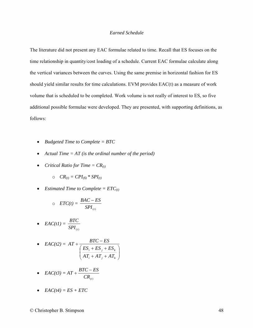
Earned Schedule
The literature did not present any EAC formulae related to time. Recall that ES focuses on the
time relationship in quantity/cost loading of a schedule. Current EAC formulae calculate along
the vertical variances between the curves. Using the same premise in horizontal fashion for ES
should yield similar results for time calculations. EVM provides EAC(t) as a measure of work
volume that is scheduled to be completed. Work volume is not really of interest to ES, so five
additional possible formulae were developed. They are presented, with supporting definitions, as
follows:
• Budgeted Time to Complete = BTC
• Actual Time = AT (is the ordinal number of the period)
• Critical Ratio for Time = CR(t)
o CR(t) = CPI($) * SPI(t)
• Estimated Time to Complete = ETC(t)
o ETC(t) = )(tSPIESBAC −
• EAC(t1) = )(tSPI
BTC
• EAC(t2) =
⎟⎟⎠
⎞⎜⎜⎝
⎛
++
++−
+
kji
kji
ATATATESESES
ESBTCAT
• EAC(t3) =)(tCRESBTCAT −
+
• EAC(t4) = ES + ETC
© Christopher B. Stimpson 48

• EAC(t5) =
⎟⎟⎠
⎞⎜⎜⎝
⎛
++
+++
kji
kji
ATATATESESES
ETCES
Following the same procedures utilized in EVM calculations, ES formulae and the EVM EAC(t)
formula were calculated and variances were derived accordingly. Slope values were then
calculated and graphed in the same fashion as the EVM calculations. As seen previously in EVM
measures, the ES measures also showed a tendency to decrease in variability as the project
progressed. Again, the values were greatly influenced by the smaller budget values at the
beginning of the project as evidenced in Figure 19.
Project TwoVariance from Actual
-60
-50
-40
-30
-20
-10
0
Apr
-00
Apr
-00
May
-00
Jun-
00
Jul-0
0
Aug
-00
Sep
-00
Oct
-00
Nov
-00
Dec
-00
Jan-
01
Feb-
01
Mar
-01
Apr
-01
May
-01
Jun-
01
Jul-0
1
Aug
-01
Sep
-01
Oct
-01
Nov
-01
Dec
-01
Jan-
02
Feb-
02
Mar
-02
Wee
ks (t
)
EAC(t1) EAC(t2) EAC(t4) EAC(t5)
Figure 11: Project Two comparison of EAC(t) formulae variance from actual.
Project Three had a flatter manpower profile than any other project. Presumably, this would lend
to greater reliability in linear calculations on non-linear data. Yet, it didn’t appear that way at
© Christopher B. Stimpson 49

first observation of the results. It seems that the earlier logic of initially smaller duration values,
influencing the EAC values, at the beginning of the job did not hold for Project Three. The
opposite is true. The logic does hold as evidenced in the scatter plot, but some values had greater
variability due to a significant negative shift of the entire manpower profile throughout its
execution.
Project ThreeVariance from Actual
-40
-30
-20
-10
0
10
20
30
40
50
60
Jul-0
0
Aug
-00
Sep
-00
Oct
-00
Nov
-00
Dec
-00
Jan-
01
Feb-
01
Mar
-01
Apr
-01
May
-01
Jun-
01
Jul-0
1
Aug
-01
Sep
-01
Oct
-01
Nov
-01
Dec
-01
Jan-
02
Feb-
02
Mar
-02
Apr
-02
May
-02
Jun-
02
Wee
ks (t
)
EAC(t1) EAC(t2) EAC(t4) EAC(t5)
Figure 12: Project Three comparison of EAC(t) formulae variances from actual.
Amazingly, EAC(t4) consistently showed its ability to more accurately predict project duration
as seen in Figure 20. In Project Three’s case, the remaining amount of work completed in the
later periods was not decreased until the very end, thus confirming the effectiveness of EAC(t4).
Recall that EAC(t) and EAC(t3) both relied on actual quantity data and the CPI($) in CR(t).
Therefore, those projects without actual period quantity data could not utilize EAC(t) and
EAC(t3) measures.
© Christopher B. Stimpson 50

Descriptive statistics were performed on all EAC(t) formulae provided by EVM and ES. They
are presented as follows:
Table 4: EAC(t) formulae descriptive statistics. EAC(t)(EVM)
N Minimum Maximum Mean Std. Deviation Variance Skewness Kurtosis
Statistic Statistic Statistic Std. Error Statistic Statistic Statistic Std. Error Statistic Std. Error
Project One 28 -0.02 0.35 0.18 0.03 0.14 0.02 -0.36 0.44 -1.38 0.86
Project Two
Project Three
Project Four 18 -0.59 0.05 -0.09 0.04 0.19 0.04 -1.99 0.54 3.00 1.04
EAC(t1)
Project One 28 -0.44 -0.03 -0.22 0.02 0.09 0.01 -0.59 0.44 1.04 0.86
Project Two 23 -0.55 -0.03 -0.08 0.02 0.10 0.01 -4.49 0.48 20.97 0.93
Project Three 23 -0.21 0.55 -0.05 0.04 0.20 0.04 1.60 0.48 2.29 0.93
Project Four 18 -0.13 0.04 -0.02 0.01 0.06 0.00 -0.61 0.54 -1.09 1.04
EAC(t2)
Project One 28 -0.39 -0.04 -0.22 0.02 0.08 0.01 -0.01 0.44 0.00 0.86
Project Two 21 -0.37 -0.04 -0.09 0.02 0.07 0.01 -3.35 0.50 12.23 0.97
Project Three 21 -0.21 0.32 -0.06 0.04 0.17 0.03 1.14 0.50 -0.13 0.97
Project Four 17 -0.92 0.03 -0.09 0.05 0.23 0.05 -3.51 0.55 13.15 1.06
EAC(t3)
Project One 28 -0.45 -0.02 -0.15 0.02 0.11 0.01 -1.18 0.44 0.69 0.86
Project Two
Project Three
Project Four 18 -0.86 -0.05 -0.32 0.08 0.32 0.10 -0.92 0.54 -1.03 1.04
EAC(t4)
Project One 28 -0.34 -0.14 -0.20 0.01 0.05 0.00 -1.52 0.44 2.11 0.86
Project Two 23 -0.54 -0.03 -0.07 0.02 0.10 0.01 -4.62 0.48 21.78 0.93
Project Three 23 -0.09 0.50 0.02 0.03 0.14 0.02 2.24 0.48 5.93 0.93
Project Four 18 -0.09 0.04 0.01 0.01 0.04 0.00 -1.61 0.54 1.62 1.04
EAC(t5)
Project One 28 -0.58 -0.11 -0.28 0.02 0.12 0.01 -0.80 0.44 0.05 0.86
Project Two 21 -0.43 -0.04 -0.10 0.02 0.09 0.01 -3.28 0.50 12.17 0.97
Project Three 21 -0.32 0.47 -0.09 0.06 0.26 0.07 1.14 0.50 -0.08 0.97
Project Four 17 -1.20 0.03 -0.14 0.07 0.30 0.09 -3.20 0.55 11.17 1.06
© Christopher B. Stimpson 51

Findings and Interpretation
Earned Value Management
It is desired to have the EAC formula with the lowest standard deviation to overcome the
difficulty faced with non-linear data. As seen in Table 6 the clear choice for use on projects for
many owners is EAC(1).
The target of EAC is the actual number of man-hours performed on a project. It is desired to be
as close as possible to this number. EAC(1) demonstrated this in the plots created. To summarize
the values, consult Table 6. The values observed were chosen from the first period to have five
percent of the total man-hours budgeted for execution.
The upper value is the largest period variance from the actual man-hours. The lower value is the
variance of the last period’s EAC from the actual man-hours. While the variances shown are
quite large by financial standards, it cannot be fully quantified whether it is sufficient for
quantities or if unit prices are needed to make EAC(1) a more viable measure. It is suggested to
explore its use when unit prices are available for use.
Table 5: Project results of EAC(1) . EAC(1)
Project Budget Actual Difference Upper Lower Project One 1,081,886 964,018 117,868 34.5% 13.4% Project Two
Project Three Project Four 705,990 824,765 -118,775 48.1% 16.5%
From first 5% month to end of project.
© Christopher B. Stimpson 52

EAC(1) does not show tremendous promise with these results. It must be remembered that it was
tested on only two projects that had actual quantity data and that it was not used with costs, as
EVM originally intended. The standard calculations accompanying EAC(1) would be used under
normal circumstances. These are described in the literature review on EVM methods.
Critical Ratio
It was observed that the formulae which relied on the CR, in their respective elements, were
unreliable and showed greater variation in the results. This appears to support Evensmo and
Karlsen’s conclusion that the CR is not based on firm theory (Evensmo and Karlsen, 2004). The
roots of variation in the CR calculated in the analysis were elusive and difficult to trace. No
conclusion of factors that influence the CR and its effects on EVM and ES formulae could be
reached. Therefore, its use should be refrained on many projects.
PMI’s TCPI Measurement
PMI presented TCPI as a potential measurement for determining how well the project must
perform through the remainder of the project. Though well intended, this measure was not
reliable and produced very misleading results. One major flaw with the formula is that it does not
take into account what will happen to the index when the BAC value is exceeded by the actual
value at that point in time. Project Four showed this flaw very clearly in Figure 21.
© Christopher B. Stimpson 53

Project FourPerformance Indices
-20
-15
-10
-5
0
5
Jul-0
2Ju
l-02
Sep
-02
Sep
-02
Oct
-02
Dec
-02
Dec
-02
Feb-
03M
ar-0
3M
ar-0
3A
pr-0
3Ju
n-03
Jun-
03Ju
l-03
Sep
-03
Sep
-03
Nov
-03
Dec
-03
Jan-
04Fe
b-04
Mar
-04
Mar
-04
May
-M
ay-
CPI(e) SPI(e) SPI(t) TCPI
Figure 13: Project Four comparison of TCPI to other indices.
To further illustrate TCPI’s inherent weaknesses, consider the initial and concluding values in
Figure 22, which are one and zero, respectively. Initial values of one are always true, as the
project has not conducted any work and remaining work must proceed at an efficiency of 1.0 to
succeed accordingly. The concluding values of zero are always true also, as the project has
completed all work and cannot proceed any longer.
© Christopher B. Stimpson 54

Project OnePerformance Indices
0
0.2
0.4
0.6
0.8
1
1.2
1.4
1.6
Jan-
02
Mar
-02
May
-02
Jul-0
2
Sep
-02
Nov
-02
Jan-
03
Mar
-03
May
-03
Jul-0
3
Sep
-03
Nov
-03
Jan-
04
Mar
-04
May
-04
Jul-0
4
Sep
-04
Nov
-04
Jan-
05
Mar
-05
May
-05
CPI(e) SPI(e) SPI(t) TCPI
Figure 14: Project One comparison of TCPI to other indices.
Yet, the concern arises when the trend shows itself to allow ever decreasing efficiency as the
schedule nears completion. Again, TCPI is bound to finite values as SV($) is. The TCPI values
will always start and end in the same place of every project, regardless of how early it is
completed and will immediately become invalid if the actual quantity exceeds the BAC. It is
concluded that TCPI not be used on many projects.
Earned Schedule
Again, it is desired to have the lowest possible standard deviation to overcome non-linear dataset
influences. According to Table 7 EAC(t)(EVM) had the highest standard deviation, largely due
to its nature of calculating only on quantities and volume of work scheduled to be completed. Of
© Christopher B. Stimpson 55

all of the EAC(t) measures, EAC(t4) had the lowest standard deviation values With Project Two
showing slight resistance to this trend.
The target of EAC(t) is the actual number of periods on a project. It is desired to be as close as
possible to this number. EAC(t4) demonstrated this in the plots created. To summarize the
values, consult Table 9. The values observed were chosen from the first period to have 5% of the
total man-hours budgeted for execution.
The upper value is the largest period variance from the actual number of periods. The lower
value is the variance of the last period’s EAC from the actual number of periods. While the
variances shown for Project One are quite large, the remaining projects have very low variances
over the middle and end of the projects.
Table 6: Project results for EAC(t4)
EAC(t4)Project Budget Actual Difference Upper Lower
Project One 196 170 26 22.4% 14.6% Project Two 93 90 3 8.0% 3.7%
Project Three 96 98 -2 8.8% 0.03% Project Four 104 108 -4 3.0% 0.50%
From first 5% month to end of project.
Project One has a large variance because of the nature of the project execution cycle and is not
the result of the EAC(t4) formula. It is concluded that EAC(t4) with it’s related variance and
index is a reliable and beneficial measure that can and ought to be used on future projects. One
strong advantage to this measure is that it does not require actual quantity data used in the EVM
formulae.
© Christopher B. Stimpson 56

Summary
It is widely recognized that different individuals prefer different levels of detail in project
metrics. This study addressed only those that can be and are produced from the project schedule.
Various metrics were found to be less than acceptable while others were found to be of great
value. EVM metrics tend to portray confusing messages because schedule progress is measured
in terms of budget – which is difficult to understand for average project managers.
Average project managers prefer to know the key performance indicators that mean something to
them. Typically the project manager can control two things in a project – time and labor. Savings
on equipment and materials typically don’t have significant impact on the bottom line.
They want to know metrics about what they can control. Fortunately, some owners use quantities
to make EVM metrics more understandable and friendly for the project manager to use.
EVM has significant limitations which were described throughout the paper. Not all is lost. The
quantity and cost variances in EVM can be converted to quantity variances that describe two
things, efficiency of actual labor versus earned labor and variance between budgeted labor versus
earned labor. These metrics can provide the project manager with great insight to how the labor
force is performing on a cumulative basis and period-to-period.
The CPI and EAC formulae will also work for labor quantities, enhancing insight to labor force
performance. But, it must be recognized that no degree of reliability of the metrics was not
present on periods with less than five percent of the BAC in the first part of the project.
© Christopher B. Stimpson 57

Reliability of the measures will increase after the first five-percent period and will decrease
slightly after the last five-percent period. During the first part of the project, diligence will be
vital as EVM metrics will not accurately describe project progress or outcome. Forecasted values
should not be used as a firm estimate in any circumstance when schedule resources are based on
quantities. Further exploration on cost loaded schedules is warranted to validate these claims.
ES is an emerging technique of measuring progress. It was explored and experimented with great
anticipation. It was found to be a viable and more accurate in time metrics than EVM. In fact, ES
will still perform well without actual manpower data. Only budgeted and earned manpower data
is necessary for ES metrics to be calculated, which is an added plus for those projects where
politics prevents reliable actual manpower data.
As was the case with EVM metrics, ES metrics are not readily reliable in the first part of the
project and increases in reliability after the first five-percent period. ES metrics do not lose
reliability as rapidly at the end of a project as evidenced in EVM metrics. Nonetheless, it must be
remembered that ES metrics are inherently influenced by project decisions to put off non-critical
tasks until later in the project. This may lead to the “growing grass” indicating that the project
will not be complete until much later than planned when, in fact, COD will be reached and the
plant will be essentially completed.
Reports
As mentioned earlier, some individuals desire to have more metrics and others desire to have
fewer metrics for reviewing project health. The balance between too much and not enough is
© Christopher B. Stimpson 58

difficult to strike. Consideration has been given to a means of presenting concise metrics that are
sufficient for everyone’s needs and do not take up a lot of space, like a dashboard of sorts. The
core components of the recommended dashboard are the key performance indicators (KPIs).
The KPIs collect and present the metrics in two categories of time and manpower. As seen in
Table 10, the key data used to calculate the metrics and the metrics themselves are placed in
logical order and side-by-side to facilitate easier review. The cells with the key metrics are
conditionally formatted to change color based on the stoplight approach to reduce the need for
individual calculation by the reviewer. The conditional formatting can be set according to a
range of acceptable thresholds much like Chang’s scale.
© Christopher B. Stimpson 59

Table 7: Project One key performance indicators.
196 weeks 1,081,886 MH118 weeks 378,385 MH
109.6 weeks 297,517 MH-8.4 weeks -80,868 MH93% 211,738 MH
141%
5 weeks 45,738 MH6.8 weeks 60,364 MH
135% 14,626 MH35,640 MH169%
203 weeks 769,961 MH93 weeks 558,223 MH
58% 27%60%
Project OneKey Performance Indicators
Schedule ManpowerCumulative Cumulative
Planned Duration Budgeted Manpower (Total)Actual Time to Date Budgeted Manpower to DateEarned Time to Date Earned Manpower to DateSchedule Variance Variance of Earned ManpowerSchedule Performance Index Spent Manpower to Date
Quantity Performance IndexPeriod Period
Time in Period Budgeted Manpower in PeriodEarned Time in Period Earned Manpower in PeriodSchedule Performance Index Variance of Earned Manpower
Actual Manpower in PeriodQuantity Performance Index
Estimate EstimateEstimated Duration Estimated ManpowerEstimate to Complete Estimate to Complete
Percent Complete Percent Complete
Estimated DurationBudgeted Duration Budgeted Manpower
Several charts were created to help formulate a modified reporting regimen to incorporate the
metrics in this study. These charts are available in Appendix A. The typical progress curves were
found to be of value for future use. But, it may be debatable to retain the forecasted early curve
and forecasted late curve. The indices tend to indicate trends of performance that can be
reasonably extrapolated within the ranges of the forecast curves, thus making them redundant.
Nonetheless, the late budgeted manpower curve was retained because of its significance as the
“lower threshold” of the project.
The traditional s-curve charts are challenging to read. They do not reveal the period-to-period
differences and only reveal cumulative progress. To facilitate review of period metrics in
comparison to other periods, a bar chart of the manpower profile was created. Now, each period
can be reviewed for budgeted, earned and actual amounts with easy comparisons to prior periods
© Christopher B. Stimpson 60

and future periods. The data that supports the bars is placed in a data table to allow access to
those who desire the data. An example of this chart is in Appendix A.
Currently some owners do not use any sort of scoring system of sorts for indicating performance.
Any scoring that takes place is limited to the s-curves and individual calculations of the
supporting data sets. Various individuals calculate their “metrics” using their own formulae and
communication roadblocks may occur. This is an area that needs improvement, which is outside
the scope of this research.
Chang’s ranges and scores for C/SPIs, as seen in Figure 5, were not applied in this research
because of its original application to engineering functions for CalTrans projects. That is not to
say that such a scale cannot be developed for an owner’s projects. If such a scale is developed, it
is important to make a scale for engineering, and one for construction and so forth. One scale
will not work for all disciplines due to the differing nature of the work in different disciplines.
This effort should take place under a separate cover from this research.
In the interim, to avert future communication roadblocks, two types of charts were developed.
Figure 23 shows a performance indices chart of the indices to date. With standard scoring
through indices project performance can be discussed using the same language and
visualizations. Anything less than one is undesirable and anything over one is desirable. The
values can also be thought of as percentages as explained in the literature review.
© Christopher B. Stimpson 61

Project OnePerformance Indices
00.20.40.60.8
11.21.41.6
Jan-
02Fe
b-02
Mar
-02
Apr
-02
May
-02
Jun-
02Ju
l-02
Aug
-02
Sep
-02
Oct
-02
Nov
-02
Dec
-02
Jan-
03Fe
b-03
Mar
-03
Apr
-03
May
-03
Jun-
03Ju
l-03
Aug
-03
Sep
-03
Oct
-03
Nov
-03
Dec
-03
Jan-
04Fe
b-04
Mar
-04
Apr
-04
Inde
x
CPI(q) SPI(t)
Figure 15: Project One performance indices.
Oftentimes managers want a one-stop measurement of performance. This is very difficult to do
with time and cost. Often the percentages of time progress and cost progress are weighted or
averaged with a certain weighting and other various ways. This leads to miscommunication and a
dangerous value that can be misleading as evidenced in the discussion about CR. To avert this
difficulty and facilitate meaningful communication with a one-stop measurement, a CPI/SPI
matrix was developed.
Figure 24 shows that Project One, at the time of reporting, was slightly late and using its labor
force efficiently to complete the earned schedule tasks to date. The quadrants are identified with
labels to help the reviewer understand what is meant when the bubble is in that quadrant. The
bubble is colored according to caution level, like the labels.
© Christopher B. Stimpson 62

Figure 16: Project One cumulative CPI/SPI matrix.
Figure 25 shows the same information for Project One’s period performance in the same
reporting period. Clearly, this indicates that sole observation of the s-curve is insufficient. The
matrix charts can supplement the manpower profile chart.
© Christopher B. Stimpson 63

Figure 17: Project One period CPI/SPI matrix.
It is believed that the use of EVM using quantities, ES metrics, and these reports will further
enhance the way owners do business. Managers will be better informed and not inundated with
countless metrics or none at all. Furthermore, consultants for lenders may be better informed
about project performance to further facilitate financing for future projects. The benefits of this
research are not quantifiable, but clearly communication can be facilitated and enhanced using
these methods for the continued success of many owners.
© Christopher B. Stimpson 64

Discussion of Potential Hypotheses
1 – EVM technique is misapplied.
In reviewing the EVM technique and its formulae, the EVM method was not really utilized by
the owner in its intended way. There were several attempts to use it and do some sort of analysis
with the data along the lines of EVM. But, none of it really came to fruition. It cannot be safely
said that it was misapplied, but maybe it could be said that it was misunderstood or under
applied.
2 – Reported values are incorrectly describing project progress.
The typically reported project progress value is the percent of manpower earned. In other cases
the percent complete is measured as a weighted formula, such as in the construction management
cost accounting (CMCA) reports. There is inconsistency in reporting percent complete. It is
difficult and faulty to make such an assumption based on time and manpower together. Percent
complete of time and manpower should be treated separately. Depending on the document and
the formulae being applied for percent complete, reported values may or may not be correct.
3 – Forecasting methods are inadequate.
Forecasting is currently done by plotting a forecast early curve and a forecast late curve that ends
up on budget and on time until the project is late. After the project is late, current forecasting
methods are considered obsolete. Currently, there are no real estimated values provided for what
the manpower will be at the end of the project or how long it will take. All that is provided for
© Christopher B. Stimpson 65

others to review is a graphical representation of work volume that is scheduled to be completed
with no respect toward SPI or CPI. Therefore, current forecasting methods are inadequate.
4 – There are better means of measuring project health and forecasting.
Testing on various projects has revealed that a more thorough use of certain EVM formulae and
the use of ES formulae yield better results for measuring project health. Furthermore, the
forecasting is more reliable than current means. While EVM forecasts are more accounting than
managerially oriented, ES forecasts are quite solid within tolerable ranges. The metrics gathered
from EVM and ES do provide a solid foundation for better reporting. Yet, the integration of SOV
values into the schedule may be of significance toward overcoming the limitations of EVM
forecasting.
EVM and ES Advancement Opportunity
In discussion with Jim zumBrunnen, Associate Director of the Statistical Laboratory at Colorado
State University, it was discovered that there may be some benefit to exploring the formulae
from a different angle. While the formulae traditionally follow the basis of original budget as
part of the calculations, it may be of value to modify the formulae to account for performance to
date and residual work using some sort of distributed weighting model. Such exploration may
increase the precision of EAC values for future use without being inhibited by the inability to use
time-series calculations (J. zumBrunnen, personal communication, October 10, 2005).
In reviewing the results of the study, zumBrunnen is in agreement that reliability of EVM and ES
formulae results is highly dependent upon completion of the first period to have 5% or more of
© Christopher B. Stimpson 66

the BAC. Furthermore, there is agreement that as the project completes, there should be more
reliable results. Yet, when there is significant interruption or shift from the baseline plans, the
results lose their credibility. It is unknown what the threshold of such shifts is and could be
explored for the benefit of being able to determine if a change in strategy is necessary for project
completion on troubled projects (J. zumBrunnen, personal communication, October 10, 2005).
EAC($) can be and is extrapolated over the remaining periods to generate an EAC($) curve.
Typically these curves are generated across the remaining periods of the BTC and not across the
remaining periods of the new ETC. If ETC is longer in duration than BTC then EAC($) will not
be extrapolated across the excess number of periods. It would seem logical to have the EAC($)
extrapolated across ETC. There is no literature to discuss this as ES is an emerging technique
that is gaining momentum, but still has not matured. Further exploration of methods to rectify
this condition is warranted.
© Christopher B. Stimpson 67

References
Anbari, F. T., PhD. (2003). Earned Value Project Management Method and Extensions. Project
Management Journal, 34(4), 12-23.
Calpine Construction Management Company, Inc. (2003). [Exhibit I – Standard Progress and
Schedule Management System]. Unpublished contract exhibit.
Chang, A.-T., PE. (2001). Defining Cost/Schedule Performance Indices and Their Ranges for
Design Projects. Journal of Management in Engineering, 17(2), 122-130.
Evensmo, J., & Karlsen, J. T., PhD. (2004). Reviewing the Assumptions behind Performance
Indices. In Transactions of AACE International: Vol. 2004. CSC.14 (pp. 1-7).
Fleming, Q. W. (1992). Cost/Schedule Control System Criteria (2nd ed.). Chicago, Illinois:
Probus Publishing Company. (Original work published 1988)
Fleming, Q. W., & Koppelman, J. M. (2000). Earned Value Project Management (2nd ed.).
Newton Square, Pennsylvania: Project Management Institute, Inc. (Original work
published 1996)
Fleming, Q. W., & Koppelman, J. M. (2003, September). What's Your Project's Real Price Tag.
Harvard Business Review, 81(9), 20-22.
Floyd, L. A., CCC, Caddell, C. P., PE, & Wisniewski, D. E., II. (2003). Application of
Appropriate Project Control Tools. In Transactions of AACE International: Vol. 2003.
CSC.04 (pp. 1-11).
Gong, D., & Rowings, J. E., Jr. (1995). Calculation of Safe Float Use in Risk-Analysis-Oriented
Network Scheduling. International Journal of Project Management, 13(3), 187-194.
Goodpasture, J. C., PMP. (2004). Quantitative Methods in Project Management. Boca Raton,
Florida: J. Ross Publishing. (Original work published 2004)
© Christopher B. Stimpson 68

Howes, R. (2000). Improving the Performance of Earned Value Analysis as a Construction
Project Management Tool. Engineering, Construction and Architectural Management,
7(4), 399-411.
Industrial Info Research (2007). Total Value of Active North American Industrial Projects
Increases 21%. Retrieved October 31, 2007, from
http://www.industrialinfo.com/showNews.jsp?newsitemID=122804
Lewis, J. P. (2002). Fundamentals of Project Management (2nd ed.). New York, New York:
AMACOM. (Original work published 2001)
Lipke, W. (2005). Connecting Earned Value to the Schedule. CrossTalk – The Journal of
Defense Software Engineering. Retrieved September 20, 2005, from US Air Force
Software Technology Support Center:
http://www.stsc.hill.af.mil/crosstalk/2005/06/0506Lipke.html
Lipke, W.,& Hendersen, K. (2005,May). Earned Schedule – an Extension to EVM Theory.
Presentation at EVA-10 Conference, London UK. Retrieved September 20, 2005, from
Project Management Institute, Sydney, Australia Chapter: http://sydney.pmichapters-
australia.org.au/programs/customer/v-filedown.asp?P=31&FID=434979427&FRF=n&
McDonald, D. F., Jr., PE CCE. (2002). Tripping Hazards in Schedules. In Transactions of AACE
International: Vol. 2003. CDR.10 (pp. 1-6).
Newell, M. W., PMP, & Grashina, M. N., PMP. (2004). The Project Management Question and
Answer Book (2nd ed.). New York, New York: AMACOM. (Original work published
2003)
Prentice, J.-P., CCE. (2003). Earned Value in the Construction and Facilities Maintenance
Environments. In Transactions of AACE International: Vol. 2003. CSC.17 (pp. 1-4).
© Christopher B. Stimpson 69

© Christopher B. Stimpson 70
Project Management Institute, Inc. (2004). A Guide to the Project Management Body of
Knowledge (PMBOK® Guide) (3rd ed.). Newton Square, Pennsylvania: Project
Management Institute, Inc. (Original work published 1996)
Project Management Institute, Inc. (2005). Practice Standard for Earned Value Management.
Newton Square, Pennsylvania: Project Management Institute, Inc.
Radosavljevic, M., & Horner, R. W. (2002). The Evidence of Complex Variability in
Construction Labour Productivity. Construction Management and Economics, 20(1), 3-
12.
Ruskin, A. M., PE. (2004). Two Issues Concerning the Use of Earned Value Measurements.
Engineering Management Journal, 16(3), 26-30.
Street, I. A., CCC. (2000). The Pitfalls of CPM Scheduling on Construction Projects. Cost
Engineering, 42(8), 35-37.
Vargas, R. V. (2003). Earned Value Analysis in the Control of Projects: Success or Failure? In
Transactions of AACE International: Vol. 2003. CSC.21 (pp. 1-4).
Webb, A. (2003). Using Earned Value. Burlington, Vermont: Gower Publishing Company.

Appendix A – Sample Dashboard Reports for Project One
196 weeks 1,081,886 MH118 weeks 378,385 MH
109.6 weeks 297,517 MH-8.4 weeks -80,868 MH93% 211,738 MH
141%
5 weeks 45,738 MH6.8 weeks 60,364 MH
135% 14,626 MH35,640 MH169%
203 weeks 769,961 MH93 weeks 558,223 MH
58% 27%60%Estimated Duration
Percent Complete Percent CompleteBudgeted Duration Budgeted Manpower
Estimated Duration Estimated ManpowerEstimate to Complete Estimate to Complete
Actual Manpower in PeriodQuantity Performance Index
Estimate Estimate
Earned Time in Period Earned Manpower in PeriodSchedule Performance Index Variance of Earned Manpower
Quantity Performance IndexPeriod Period
Time in Period Budgeted Manpower in Period
Schedule Variance Variance of Earned ManpowerSchedule Performance Index Spent Manpower to Date
Actual Time to Date Budgeted Manpower to DateEarned Time to Date Earned Manpower to Date
Cumulative CumulativePlanned Duration Budgeted Manpower (Total)
Project OneKey Performance Indicators
Schedule Manpower
© Christopher B. Stimpson 71

Project OneManpower Curves
0100200300400500600700800900
100011001200
Jan-
02Fe
b-02
Mar
-02
Apr-
02M
ay-0
2Ju
n-02
Jul-0
2Au
g-02
Sep-
02O
ct-0
2N
ov-0
2D
ec-0
2Ja
n-03
Feb-
03M
ar-0
3Ap
r-03
May
-03
Jun-
03Ju
l-03
Aug-
03Se
p-03
Oct
-03
Nov
-03
Dec
-03
Jan-
04Fe
b-04
Mar
-04
Apr-
04M
ay-0
4Ju
n-04
Jul-0
4Au
g-04
Sep-
04O
ct-0
4N
ov-0
4D
ec-0
4Ja
n-05
Feb-
05M
ar-0
5Ap
r-05
May
-05
Jun-
05Ju
l-05
Aug-
05Se
p-05
Oct
-05
Perio
d M
an-h
ours
x10
00
BQWS Cum. Lower Threshold BQWP Cum. AQWP Cum.
© Christopher B. Stimpson 72

Project OneManpower Profiles
0
20
40
60
80
100
120Pe
riod
Man
-hou
rs x
1000
BQWS Profile BQWP Profile AQWP Profile
BQWS Profile 2 3 2 3 2 2 3 2 2 3 3 7 6 7 8 14 8 5 6 7 46 33 32 57 28 42 46 42 56 98 95 93 91 61 59 30 20 13 6 5 6 10 6 7 5
BQWP Profile 2 3 2 3 2 2 3 2 2 3 3 6 4 3 3 8 4 1 0 10 24 19 19 28 35 43 60
AQWP Profile 2 3 2 3 2 2 3 2 2 3 3 6 4 4 4 8 4 1 0 2 14 16 17 21 17 29 36
J-02
F-02
M-02
A-02
M-02
J-02
J-02
A-02
S-02
O-02
N-02
D-02
J-03
F-03
M-03
A-03
M-03
J-03
J-03
A-03
S-03
O-03
N-03
D-03
J-04
F-04
M-04
A-04
M-04
J-04
J-04
A-04
S-04
O-04
N-04
D-04
J-05
F-05
M-05
A-05
M-05
J-05
J-05
A-05
S-05
O-05
© Christopher B. Stimpson 73

Project OnePerformance Indices
00.20.40.60.8
11.21.41.6
Jan-
02Fe
b-02
Mar
-02
Apr
-02
May
-02
Jun-
02Ju
l-02
Aug
-02
Sep
-02
Oct
-02
Nov
-02
Dec
-02
Jan-
03Fe
b-03
Mar
-03
Apr
-03
May
-03
Jun-
03Ju
l-03
Aug
-03
Sep
-03
Oct
-03
Nov
-03
Dec
-03
Jan-
04Fe
b-04
Mar
-04
Apr
-04
Inde
x
CPI(q) SPI(t)
© Christopher B. Stimpson 74

© Christopher B. Stimpson 75
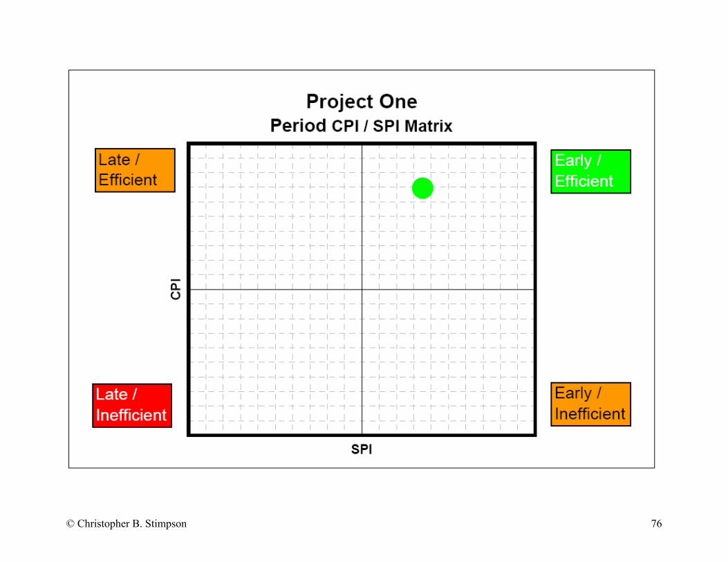
© Christopher B. Stimpson 76

© Christopher B. Stimpson 77

Glossary of Terms
Activity:
Activities are the fundamental work elements of a project. They are the lowest level of a
work breakdown structure (WBS) and, as such, are the smallest subdivision of a project.
Activity Relationship:
A relationship defines how an activity relates to the start or finish of another activity or
assignment.
Activity String:
A user-selected portion of the activity network that contains activities and their
relationships.
Actual Cost of Work Performed (ACWP):
Actual Cost is the actual total cost incurred on the activity as of the project data date.
Actual Variance:
The difference between the earned value and the actual value in EVM and ES techniques.
Backward Pass:
The set of calculations in CPM or PERT that works backwards from the ending activity
to the beginning activity to determine the late start, late finish, and float values for each
activity.
Baseline Schedule:
The schedule that is established as the target or original work plan as determined by the
project team before the work is executed.
Bell Curve:
A curve that takes the shape of a bell as typically seen in a manpower profile.
© Christopher B. Stimpson 78

Budget at Completion (BAC):
Budget At Completion is the budgeted total cost through activity completion.
Budgeted Cost of Work Performed (BCWP):
Budgeted Cost of Work Performed is the portion of the budgeted total cost of the activity
that is actually completed as of the project data date.
Budgeted Cost of Work Scheduled (BCWS):
Budgeted Cost of Work Scheduled is the portion of the budgeted total cost of the activity
that is scheduled to be completed as of the project data date.
CalTrans:
The short name given to the California Department of Transportation.
Central Limit Theorem:
One of many statistics theorems which is much applied in sampling and which states that
the distribution of a mean of a sample from a population with finite variance is
approximated by the normal distribution as the number in the sample becomes large.
Chaotic System:
A collection of non-linear data that shows no readily apparent pattern or outcome without
sophisticated mathematical analysis.
Chaos Theory:
A theory that uses non-linear data to predict complex behavior through a mathematical
algorithm.
College of Performance Management:
A separate membership organization within PMI focusing on developing tools,
techniques, and practices in the area of earned value management.
© Christopher B. Stimpson 79

Comma Separated Value File (CSV):
A text file that uses a comma to separate each and every value for importing into
spreadsheet programs or other applications.
Commercial Operation Date (COD):
The date a manufacturing facility is available for immediate production.
Commissioning:
Testing and check-out of systems for completeness and readiness for startup.
Commodities:
Non-labor resources that are utilized or consumed on a project such as a pipe, concrete,
cable and etc.
Constraints:
Constraints are network modifications that override the natural flow of network
calculations to show the desired project situation.
Construction Management:
A project delivery system that uses a construction manager to facilitate the design and
construction of a project by organizing and directing men, materials, and equipment to
accomplish the purpose of the designer. A professional service that applies effective
management techniques to the planning, design, and construction of a project from
inception to completion for the purpose of controlling time, cost and quality, as defined
by the Construction Management Association of America (CMAA).
Construction Manager (CM):
© Christopher B. Stimpson 80

A firm or business organization with the expertise and resources to manage the design,
contracting, and construction aspects of project delivery. Individuals who work for a CM
Firm are also referred to as Construction Managers.
Converge:
To come together to one activity or one path.
Cost Performance Index (CPI):
The index that describes the performance of a project in terms of cost.
Cost Variance (CV):
The difference in cost values between work performed and actual costs. This indicates
low or high efficiency.
Cost/Schedule Control Systems Criteria (C/SCSC):
The DoD standard for measuring project progress in terms of cost. It is a standard that is
included in the Acquisition Rules at the DoD.
CPI/SPI Matrix:
A matrix that shows the relationship of CPI to SPI at any point in time.
Critical Path:
The critical path is a series of activities that determines a project's completion time.
Project management software allows the user to define what rules to follow for
determining the critical path.
Critical Path Analysis (CPA):
A method of analyzing the critical path for validity and identification of issues or
opportunities.
Critical Path Method (CPM):
© Christopher B. Stimpson 81

A calculation method that is applied to a network diagram for the purpose of determining
activity start and finish dates among other desired data. This method differs from PERT
but uses the same network diagramming principles.
Critical Ratio (CR):
The product of CPI and SPI that attempts to describe the success of a project at any point
in time with one value.
Critical Task:
An activity that is on the critical path according to rules established by the project
management software and user settings.
Custom Data Item:
User-defined fields that enable the addition of custom fields and values to the project
database in P3.
Dashboard:
A simple and uncluttered place for management to retrieve essential project or portfolio
information that pertains to their area of focus.
Degrees of Freedom:
The number of project variables that are free to vary while all other project variables are
not free to vary without impacting the desired outcome of a project.
Department of Defense (DoD):
An administration in the US government whose primary objective is to defend the US
through development, acquisition, maintenance, and use of military forces.
Distribution:
The position, arrangement, or frequency of occurrence over time.
© Christopher B. Stimpson 82

Diverge:
To separate into many paths or activities from one path or activity.
Early Finish:
The earliest date an activity can complete.
Early Start:
The earliest date an activity can begin after its predecessors have completed.
Earned Duration:
A technique of measuring variance in schedule values over time as opposed to cost or
quantity.
Earned Schedule (ES):
A technique of measuring variance in schedule values over time as opposed to cost or
quantity.
Earned Standards Method:
A technique of measuring activity completion through a system of standard components
and weighting for the components.
Earned Value Management (EVM):
The technique of measuring variance in schedule values over cost or quantity as opposed
to time.
Efficiency:
The relationship between budgeted work performed and actual work performed. This
indicates the effectiveness of effort expended to complete tasks.
Effort:
TPM defines effort as the total man-hours required to complete a task.
© Christopher B. Stimpson 83

Equivalent Units:
A technique of measuring activity completion through one-to-one relationship of resource
units.
Estimate at Completion (EAC):
The estimated cost or duration of the project at completion.
Estimate at Completion Variance (EACV):
The difference between the BAC and the EAC.
Estimate to Complete (ETC):
The estimated cost or duration to complete a project.
Ex Post Facto:
After the fact. Ex post facto also describes the condition under which the data is being
studied.
Exhibit I:
An attachment to construction agreements that outline project control guidelines.
Float:
The number of days an activity or activity string can be delayed without impacting the
project completion date.
Forecasted Early Curve:
The s-curve that represents the earliest the remaining project activities can complete.
Forecasted Late Curve:
The s-curve that represents the latest the remaining project activities can complete
without impacting the project completion date.
Forward Pass:
© Christopher B. Stimpson 84

The set of calculations in CPM or PERT that works forwards from the beginning activity
to the ending activity to determine the early start, early finish, and float values for each
activity.
General Contractor (GC):
A properly licensed individual or company having "primary" responsibility for the work.
A GC can perform work with its own contractors or can perform the project work as an
independent contractor, providing services to owners through the use of subcontractors
when using the general contracting system.
Global Change:
A P3 feature that enables a user to change selected project data or the entire database
using if/then/else logic.
Industrial Construction:
Construction that deals with the design, improvement, and installation of integrated
systems in industry.
Inputs:
PMI defines inputs as requirements for a process to provide an output.
Key Performance Indicator (KPI):
The most important and relevant metrics that identify performance of a project.
Labor Productivity:
The rate at which commodity units are being expended by the associated man-hours.
Late Budgeted Manpower Curve:
The s-curve that represents the latest all project activities can complete without impacting
the project completion date.
© Christopher B. Stimpson 85
Late Finish:
The latest date an activity can finish without impacting the project completion date.
Late Start:
The latest date an activity can begin after its predecessors have completed.
Level One Schedule:
Exhibit I defines a Level One schedule as one which represents the overall general
requirements of the project, outlining the general flow of work activities - delineating the
major project milestones and commercial contract commitments.
Level Two Schedule:
Exhibit I defines a Level Two schedule as one which includes sufficient detail to
represent those relationships where the impact of execution for a given contractor or
party has a direct influence on other parties represented in the Project.
Level Three Schedule:
Exhibit I defines a Level Three schedule as one which incorporates the additional detail
beyond level two, required to manage the expenditure of significant quantities of labor
and commodities.
Longest Path:
A rule in project management software that determines how to derive the critical path
through a project.
Lump Sum Agreement:
A written agreement in which a specific amount is set forth as the total payment for
completing the contract.
Man-hour (mh):
© Christopher B. Stimpson 86

A unit of measure that describes effort of a worker to time. One worker will execute one
hour of work for each man-hour.
Manpower:
The collective effort of all workers.
Manpower Profile:
The graphical representation of manpower as related to time.
Merge Point:
An activity or milestone in a schedule network that has two or more predecessors that can
influence its finish date.
Microsoft Project:
A project management software package that is developed, marketed, and supported by
Microsoft Inc.
Milestone:
A zero duration activity that indicates completion of a desired activity string, phase, or
otherwise important segment of a project.
National Aeronautics and Space Administration (NASA):
An administration within the US government that concerns itself with the realms of
outer-space and technology advancement in communications, weather, and intergalactic
research.
Near-critical Float:
Float that a near-critical activity has.
Near-critical Path:
The path of activities that has potential of becoming critical.
© Christopher B. Stimpson 87

Near-critical Task:
A task that is not on the critical path, but has potential of becoming critical and entering
the critical path.
Non-critical Task:
A task that is not on the critical path.
Normal Curve:
A graphical representation of the normal distribution.
Normal Distribution:
A probability density function that approximates the distribution of many random
variables.
Out-of-sequence Logic:
Activity relationships that are no longer valid because of out-of-sequence progress.
Out-of-sequence Progress:
When an activity starts or completes before its predecessors are completed.
Path:
A collection of activities that are linked together with relationships. A path can take any
direction through the schedule and is not limited to specific parameters other than having
immediate relationships between activities.
Pareto Distribution:
Pareto distribution is a power law probability distribution found in a large number of real-
world situations. This distribution is also known, mostly outside economics, as the
Bradford distribution. This idea is sometimes expressed more simply as the Pareto
© Christopher B. Stimpson 88

principle or the "80-20 rule" which says that 20% of the population owns 80% of the
wealth.
Planned Value Rate:
A technique of measuring variance in schedule values over time as opposed to cost or
quantity.
Planner:
An individual who devises or projects the realization or achievement of a plan or a
program.
Population:
An entire set of objects, observations, values, or scores that have something in common.
Precedence Diagramming Method (PDM):
Also known as the activity-on-node method. This method uses a node (geometric shape)
to represent activities with connecting lines to show the logic or sequence of activities.
Predecessor:
An activity that precedes another.
Primavera:
The short name for Primavera Systems, Inc. who develops, markets, and supports project
management software.
Primavera Project Planner (P3):
A planning software package for project management that is designed, marketed and
supported by Primavera Systems, Inc. P3 has been succeeded with Primavera 6.0 (P6)
which provides substantially greater capability than P3.
Probability Calculation:
© Christopher B. Stimpson 89

A calculation to determine the probability of an occurrence.
Program Evaluation and Review Technique (PERT):
A calculation method that is applied to a network diagram for the purpose of determining
activity start and finish dates among other desired data. This method differs from CPM in
that it uses three-point estimation, but uses the same network diagramming principles.
Progress:
The act of recording actual dates and resource values as the project progresses toward
completion.
Project Controls Group (PCG):
A group of planning and control specialist that plan and monitor construction projects.
Project Management Institute (PMI):
A non-profit organization dedicated to the advancement and development of project
management as a best practice in all industries.
Rebaseline:
To make a new baseline plan when the original baseline plan is no longer valid due to
scope change or any other significant event after the project has begun execution.
Reporting Period:
A predetermined period of time that defines the beginning and end of data collection for
reporting.
Resource:
A source of materials or manpower needed to complete a project.
Resource Loading:
The assignment of resources to activities.
© Christopher B. Stimpson 90

Rework:
To work again or execute again. Rework is the product of incorrectly performed work
that must be corrected.
Rolling Wave Planning:
Rolling wave planning is a phased iterative approach to project planning. As a project
begins there may be a lack of detailed information. As the detail is received, it is added to
the project plan in waves.
S-curve:
The curve that represents cumulative values of a resource over time.
Sample:
A subset of a population that adequately represents the whole population.
Schedule Network:
The visual representation of PDM. It contains activities defined in a shape while they are
linked by lines to show relationships.
Schedule of Values (SOV):
(1) The breakdown of a lump sum price into sub-items and sub-costs for identifiable
construction elements, which can be evaluated by examination for contractor progress
payment purposes. (2) A statement furnished by the contractor to the architect or engineer
reflecting the portions of the contract sum allotted for the various parts of the work and
used as the basis for reviewing the contractor's applications for progress payments.
Schedule Performance Index (SPI):
A value that indicates the rate at which work is being completed.
Schedule Variance (SV):
© Christopher B. Stimpson 91
The difference between the work performed and the work budgeted to be completed. This
is an indicator of early or late completion.
Sensitivity:
Sensitivity is a measure of the correlation between the plan cost/duration and a task
cost/duration. The correlation is calculated using Spearman's rank order correlation
factor.
Skew:
An indication that the distribution is shifted right or left of the middle of a normal
distribution.
SPSS:
Predictive analytics software developed, marketed, and supported by SPSS Inc.
Standard Deviation:
How a much a variable deviates from the mean. Assumes the distribution is normal and
not skewed. It is calculated as the square root of the variance.
Startup:
The actual starting of equipment and systems in combined operations.
Successor:
An activity that succeeds another.
Tabular Report:
A report produced from P3 that is tabular in nature.
Task:
Also an activity.
Time Series:
© Christopher B. Stimpson 92

A sequence of observations which are ordered in time or space.
To-complete Performance Index (TCPI):
TCPI helps determine the efficiency that must be achieved on the remaining work for a
project to complete on time and within budget.
Turnkey:
Supplied, installed, or built in a condition ready for immediate use, occupation, or
operation.
Turnover:
The formal transfer of responsibility for a system from the construction phase to the
commissioning phase.
Variance:
A measure of how much the distribution is spread from the mean. A high variance
indicates results are spread out. It is the average of the squared distance of all generated
values from their mean.
Variance at Completion (VAC):
The difference between the actual cost or time and the budgeted cost or time. This
indicates overrun or underrun.
Work Volume: The quantity of work as related to time.
© Christopher B. Stimpson 93


