
The Treatment-Effect Estimation:
A Case Study of The 2008 Economic Stimulus Package of China
Min Ouyang∗
School of Economics and ManagementTsinghua University, Beijing, 100084 China
Yulei PengDepartment of Economics, University of Arkansas
Fayetteville, Arkansas 72701-1201 US
December 2013
Abstract
In 2008, the Chinese government put forth an economic stimulus package of 586 billion USD to
minimize the impact of the global financial crisis. This is considered as one of the most important
macroeconomic policy interventions in the past decade. This paper employs this policy intervention
as a case study to address the challenge of evaluating the treatment effects under time-varying latent
factors. In particular, we return to the framework of Hsiao, Ching, and Wan (2012), relax their
linear conditional mean assumption, and extend it to a semi-parametric setting. The asymptotic
distribution properties of the average treatment effect estimator is derived and studied. Both the
linear model and the semi-parametric model are applied to study the treatment effect of the 2008
stimulus package on China’s macroeconomy. The estimation results show the stimulus package had
raised the annual real GDP growth in China by about 3.2%, but only temporarily. These results
are robust to linear setting, semiparametric setting, and various control group selections. The
temporary boost in macroeconomic outcome is also evident in the estimation of other economic
indicators such as real investment, real consumption, real export, and real import.
JEL codes: C10, H73, H22.
Key words: treatment effects, stationary data, 2008 economic stimulus plan of China, parametric
estimation, semi-parametric estimation
∗The corresponding author: Min Ouyang. Email: [email protected]. We thank Qi Li and Cheng Hsiao forhelpful comments and ChongEn Bai for insightful discussions. Zhe Lu, Matthew Kidder, and Meng Li provided excellentresearch assistance. Some of the data is provided by Bing Li. Errors are ours.
1
1 Introduction
Researchers usually face the challenge of estimating the counterfactuals when evaluating the conse-
quences of policy interventions. As a case study, consider one of the most significant macroeconomic
policy interventions in the past decade: China’s 2008 economic stimulus package. Starting from the
end of 2008, the central Chinese government put forth an economic stimulus package of four trillion
RMB – equivalent to 586 billion USD, about three times size of the U.S. stimulus package at the
time– as an attempt to minimize the impact of the global financial crisis. The influence of this policy
intervention has been much debated among policy makers; therefore, estimating its treatment effect
on China’s macroeconomy would provide intriguing evidence for future policy discussions. However,
in evaluating this policy, simply comparing China’s macroeconomic outcome before and after the end
of 2008 would not be sufficient, because the post-treatment outcome is under the influence of many
factors other than China’s stimulus package. Such factors can be, for example, weather, trade devel-
opment, population growth, technological advancements, or other governments’ policy interventions.
All these factors vary before and after the end of 2008 and, most importantly, their variations are ei-
ther unobservable, unmeasurable, or very difficult to control for. Therefore, the counterfactuals – the
hypothetical macroeconomic outcome of China in the absence of the 2008 stimulus package – become
the key element in estimating the treatment effects of this policy intervention.
There are several ways to construct the counterfactuals with time-varying latent factors. One can
estimate a latent factor model as suggested by Bai and Ng (2002). Unfortunately, this method applies
only when both the cross-section and the time-series dimensions are sufficiently big, which is rarely
the case when evaluating macro policies. Or, one can perform a time-series prediction by estimating
a VAR model. But a VAR prediction cannot incorporate any post-treatment shocks as its prediction
is out of the sample. Alternatively, one can use data changes in a group of regions not under the
policy intervention to control for the time-varying latent factors. This is the conventional difference-
in-difference (hereafter DID) approach (Card and Krueger, 1994). However, the DID is subject to
quite a few restrictive assumptions: first, the treatment assignment must be random (no selection
bias); second, the treatment and control regions must share the same latent factors; third, common
latent factors must have the same quantitative influence on each group so that taking differences
removes the effects. These assumptions are hard to maintain in applied work because, in reality,
policy makers’ choice of the treatment region is never random. Most importantly, regions differ in
terms of demographics, culture, and economic and political institutions, so that most latent factors as
well as their influences do vary cross-section. Failure to incorporate such cross-section heterogeneity
can severely bias the estimates. One can also use the synthetic control method proposed by Abadie
2
and Gardeazabal (2003) and Abadie, Dimond, and Hainmueller (2010) to estimate averae treatment
effects. The synthetic control method relaxes the equal weight restriction of the DID method. However,
when the treated unit and the control units exhibit different trending behaviors (in the absent of
treatment), the synthetic control method may result in poor in-sample-fit, in such cases the synthetic
control method should not be used (Abadie, Dimond, and Hainmueller 2010, page 495).
Hsiao, Ching, and Wan (hereafter HCW) (2012) initiate an approach that offers more flexibilities
than the DID and the synthetic control methods. They propose to estimate the correlations between
the treatment and control regions based on the pre-treatment data. In this way, regions that display
strong correlations should share common latent factors with the treatment region. More importantly,
estimating the correlations rather than taking simple differences allows the influence of common latent
factors to vary cross-section. This makes the approach much more applicable to reality. Bai, Li, and
Ouyang (2014) extend the HCW approach to the case with non-stationary data and prove that, as long
as the data follows I(1), the OLS estimator of the correlation coefficient is the unique and consistent
estimator that can uncover the post-treatment counterfactuals using the post-treatment observations
of the control regions.
In this paper, as a first step we return to the original framework of HCW (2012). HCW (2012)
method relies on a key assumption that the conditional mean of the error term is a linear function of the
latent factors (Assumption 6); otherwise the consistency of the OLS estimator cannot be established.
We relax this assumption by allowing the conditional mean to have a semi-parametric setting. We
show that, under quite general conditions as those in Robinson (1988) and Fan and Li (1999), one can
consistently estimate the counterfactuals and can therefore uncover the true treatment effects.
Accordingly, we adopt the HCW framework to estimate the conterfactual macroeconomic outcome
of China in the absence of the 2008 stimulus package. In selecting control economies, we look for those
that not only display strong correlations with the Chinese economy, but are relatively independent
of the 2008 stimulus package post-treatment. More specifically, we examine the trade relationships
between China and potential control economies. Economies whose total trade volume with China
constitutes only a small fraction of their own GDP should be relatively independent of any policy
interventions implemented in China. Hereby we maintain an important assumption by HCW(2012)
that the policy intervention must remain exogenous to the control group.
Applying both the parametric and semi-parametric settings, we estimate that the 2008 stimulus
package had raised the annual real GDP growth in China by about 3.2%, but only temporarily. In
particular, the estimated post-treatment counterfactual growth is 3.2% lower than the actual growth;
however, our results show that the counterfactual and actual growth coincide with each other starting
3

from about two years after the policy intervention. This suggests the stimulus package had a temporary
growth effect of 3.2% on China’s real GDP for about two years. These results remain robust to
linear setting, semi-parametric setting, and various control group selections. The temporary boost in
economic activities of the stimulus package is also evident in the estimation of other macroeconomic
indicators such as real investment, real consumption, real export, and real import.
The rest of the paper is organized as follows. Section 2 presents the model set up and extends the
model to a semi-parametric setting. Section 3 applies the model to estimate the 2008 Fiscal Stimulus
Plan of China. We conclude in Section 4.
2 The Model
Let y1it and y0
it denote unit i’s outcome in period t with and without treatment, respectively. The
treatment intervention effect for the ith unit at time t is defined as
∆it = y1it − y0
it. (1)
However, often we do not simultaneously observe y0it and y1
it. The observed data are in the form
yit = dity1it + (1− dit)y0
it, (2)
where dit = 1 if the ith unit is under the treatment at time t, and dit = 0 otherwise.
Let ft be a K × 1 vector of unobservable common factors which is the main force that drives all
the yit to change over time. Following Hsiao, Ching and Wan (2012), in this paper we assume that ft
is strictly stationary process.1 We consider the case that there is no treatment to yit for all i and for
t = 1, ..., T1. For t = T1 + 1, ..., T there is one unit, say the first unit without loss of generality, that
goes through a treatment, but all other unit yjt, j = 2, ..., N , still do not endure any treatment. So
there is no treatment for yjt for j = 2, ..., N and for all t = 1, ..., T .
Following HCW (2012) we consider the following factor model
y0it = αi + b′ift + uit, i = 1, ..., N ; t = 1, ..., T1, (3)
where αi is unit i’s individual specific intercept, bi is a K×1 vector of factor loading, uit is a stationary
I(0) error term.
Let yt = (y1t, ..., yNt)′ be an N × 1 vector of yit at time t. Since there is no policy intervention
1The case that ft is non-stationary is considered by Bai, Li and Ouyang (2012).
4

before T1, then the observed yt takes the form
yt = y0t = α+Bft + ut for t = 1, ..., T1, (4)
where α = (α1, ..., αN )′, B is a N ×K matrix with the ith row given by b′i, and ut = (u1t, ..., uNt)′.
Since at time T1 + 1, there is a policy change to the first unit, hence, from time T1 + 1 on we have
y1t = y11t for t = T1 + 1, ..., T . (5)
We assume that other units are not affected by the new policy implemented to the first unit.
Therefore,
yit = y0it = αi + b′ift + uit, for i = 2, ..., N , and t = 1, ..., T . (6)
Since y01t is not observable for t ≥ T1 + 1, we need to estimate the counterfactual outcome y0
1t. If
T and N are large, the method of Bai and Ng (2002) identifies the number of common factor, K, and
estimates ft along with B by the maximum likelihood approach. Hsiao, Ching and Wan (2012) (HCW,
hereafter) suggest an alternative method by using Yt = (y2t, ..., yNt)′ in lieu of ft to predict y0
1t for
post-treatment period t. The validity of HCW’s approach depends on a linear conditional expectation
function assumption, if the conditional mean function is not a linear function, their proposed estimator
may not lead to consistent estimation of the average treatment effects. In this paper we will generalize
HCW’s method to allow for flexible conditional mean function form so that we can consistently estimate
the average treatment effects robust to functional form misspecification.
2.1 The Parametric Regression Model
In this subsection we discuss HCW’s proposed estimation method. Recall that yt = (y1t, Y′t )′, where
Yt = (y2t, ..., yNt)′. The pre-treatment data y0
t is generated by the factor model
y0t = α+Bft + ut, for t = 1, ..., T1, (7)
where α = (α1, ..., αN )′, and B is a N×K factor loading matrix, and ft is the unobserved K×1 vector
of common factors, ut is a N ×1 idiosyncratic I(0) error. Let a = (1,−γ′)′ where γ = (γ2, ..., γN )′ such
that a′B = 0, i.e., a ∈ N (B), where N (B) is the null space of B. Then we have that
a′yt ≡ y1t − γ′Yt = a′α+ a′ut
5
because a′B = 0 so that the common factors are dropped out from the right-hand-side of the above
equation. Rearranging terms we obtain
y1t = γ1 + γ′Yt + u∗1t, (8)
where γ1 = a′α and u∗1t = a′ut = u1t − γ′Ut with Ut = (u2t, ..., uNt)′.
Because u∗1t depends on all the ujt for j = 1, ..., N , obviously, u∗1t and Yt are correlated. We can
decompose u∗1t as u∗1t = E(u∗1t|Yt) + ε1t, where ε1t = u∗1t − E(u∗1t|Yt) and E(ε1t|Yt) = 0. Then we can
re-write (8) as
y1t = γ1 + γ′Yt + E(u∗1t|Yt) + ε1t. (9)
HCW further assume that (linear conditional mean function assumption)
E(u∗1t|Yt) = a0 + b′0Yt. (10)
Equation (10) is in fact equivalent to Assumption 6 of HCW (2012).
Replacing E(u∗1t|Yt) in (9) by (10), we obtain
y1t = δ1 + δ′Yt + ε1t, (11)
where δ1 = γ1 + a0 and δ = γ + b0. Because E(ε1t|Yt) = 0 (this follows the definition of ε1t, which
follows from E(u∗1t|Yt) is linear in Yt), hence, OLS regression of y1t on (1, Y ′t ) will lead to consistent
estimate of (δ1, δ′)′.
Let (δ1, δ′) denote the OLS estimator of (δ1, δ
′) based on (11), HCW suggest to use
y01t = δ1 + Y ′t δ, t = T1 + 1, ..., T,
to predict the counterfactual outcome y01t. Then the average treatment effects is estimated via
T−12
∑Tt=T1+1 ∆1t, where T2 = T − T1 and ∆1t = y1t − y0
1t.
However, the linear conditional mean functional form (10) is restrictive,2 and a misspecified re-
gression functional form may lead to inconsistent estimation result for the treatment effects.
2.2 The Semi-parametric Regression Model
In this subsection we discuss how to relax the linear conditional mean function assumption. Without
imposing assumption (10) we can write (9) as
y1t = g(Yt) + ε1t, (12)
2When ft and ut are jointly normally distributed, yt is jointly normally distributed and (10) holds true, however,when ft and ut are not jointly normally distributed, (10) may not hold in general.
6
where g(Yt) = γ1 + γ′Yt + E(u∗1t|Yt). The functional form g(·) is not known if the functional form
E(u∗1t|Yt) is unspecified. Nevertheless, we can estimate g(·) using some standard nonparametric esti-
mation method, say by the local constant kernel method.
g(Yt) =
∑T1s=1 y1sK1s,2t∑T1s=1K1s,2t
, t = T1 + 1, ..., T (13)
where K1s,2t =∏Nj=2 k((y1s − yjt)/hj) is the product kernel function, hj is the smoothing parameter
associated with covariate yjt for j = 2, ..., N . The average treatment effects is then estimated by
∆1,NP =1
T2
T∑t=T1+1
[y1t − g(Yt)] . (14)
When N is not small, the above estimator suffers the ‘curse of dimensionality’ problem. Alterna-
tively, one may use some semi-parametric regression function to approximate g(·), say g(Yt) = β′z1t +
θ(z2t), where z1t and z2t are non-overlapping variable and their union forms Yt, i.e., Y ′t = (z′1t, z′2t).
Let q be the dimension of z2t, when z2t’s dimension q is low, the ‘curse of dimensionality’ problem
is greatly ameliorated. We can use the method of Robinson (1988) to estimate the partially linear
model. In fact, one can view that the partially linear model includes both a linear model and a general
nonparametric model as special cases. It give rise to a linear model if z1t = Yt and z2t is an empty set
of covariate, and it leads to a nonparametric regression model when z2t = Yt and z1t is an empty set.
Let β and θ(z2t) denote the semi-parametric estimators of β and θ(z2t), respectively, using the
pre-treatment data (say using the estimation method proposed by Robinson (1988)), or the estimators
proposed by Fan and Li (1999) who consider weakly dependent data case. Under quite general condi-
tions Robinson (1988) and Fan and Li (1999) show that β − β = Op(T−1/21 ). Then the counterfactual
outome y01t is estimated by y0
1t = z′1tβ + θ(z2t) for t = T1 + 1, ..., T , and the average treatment effects
is estimated by
∆1,PL =1
T2
T∑t=T1+1
[y1t − z′1tβ − θ(z2t)
]. (15)
We will show that ∆1 consistently estimates the sample mean of ∆1t (i.e., ∆1 = T−12
∑Tt=T1+1 ∆1t)
whether ∆1t is stationary or not. In the case that ∆1t is a strictly stationary process, ∆1 consistently
estimates the population mean ∆1 = E(∆1t).
To establish the consistency of ∆1, we need to make some regularity assumptions. We will consider
β-mixing process. Let {Wt} ≡ {yt, ft} be strictly stationary β-mixing process, i.e., as τ →∞,
βτ = sups∈N
E
{sup
A∈M∞s+τ (W)
[|P (A|Ms
−∞(W))− P (A)|]}→ 0,
7
where Mts(W) denotes σ(Ws, ...,Wt), the sigma algebra generated by (Ws, ...,Wt), for s < t.
We will use the class of kernel functions Kl for some positive integer l, and the class of smooth
functions Gαµ introduced by Robinson (1988). For readers’ convenience, we restate these two definitions
here.
Definition 1 Kl, l ≥ 2, is the class of even functions k: R → R satisfying∫Rvik(v)dv = δi0 (i = 0, 1, ..., l − 1)
k(v) = O((1 + |v|l+1+δ)−1), for some δ > 0,
where δij is the Kronecker’s delta.
Definition 2 Gαµ , α > 0, µ ≥ 1 is a positive integer, is the class of functions g: R → R satisfying: g
is µ-time partially differentiable, for some ρ > 0, supy∈φzρ |g(y) − g(z) − Qg(y, z)| ≤ G(z)|y − z|µ for
all z, where φzρ = {y : |y − z| < ρ}; Qg is a (µ − 1)th degree homogeneous polynomial in y − z with
coefficients the partial derivatives of g at z of orders 1 through µ− 1; g(z) and its partial derivatives
of order µ− 1 and less, and Gg(z) all have finite αth moments.
Definition 1 characterizes the class of (possibly higher order) kernel functions. When l > 2, k is
a higher order kernel function which often used to reduce nonparametric estimation bias. Definition
2 imposes smoothness and moments conditions on function g ∈ Gαµ . It means that g is differentiable
up to order µ and has a Taylor expansion given by [g(z) +Qg(y, z)] with remainder satisfying a local
Lipschitz conditions. Also, g and its partial derivative functions (up to order µ) all have finite αth
moments.
Recall that f(·) is the density function of z2t, ξt = E(z1t|z2t). Define ηt = z1t−E(z1t|z2t), we make
the following assumptions.
Assumption A1. (i) {yt, ft}, t = 1, ... is a strictly stationary β-mixing process with the mixing
coefficient βτ satisfying βδ/(1+δ)τ = O(τ−2+ε) for some 0 < ε < 1, 0 < δ ≤ 1/2 and qδ/(1 + δ) < 2.
Assumption A2. f ∈ G∞ν−1, g ∈ G4ν , where ν ≥ 2 is a positive integer. Also, g and ξ all satisfy some
(global) Lipschitz conditions: |θ(y) − θ(z)| ≤ Dθ(z)|y − z| for all y, z ∈ Rq, where Dθ has finite 4th
moments and θ = f , g, ξ.
Assumption A3. ε1t is a martingale difference process, E(ε4+δ1t ) < ∞ and E(η4+δ
j ) < ∞ for some
δ > 0, where ηj is the jth component of η for j = 1, ..., N−q. Also, σ2(z1, z2) = E(v2t |z1t = z1, z2t = z2)
and σ2v(z2) = E(v2
t |z2t = z2) both belong to G21 , where vt = ε1t or ηjt, j = 1, ..., N − q.
8
Assumption A4. (i) k ∈ K2. (ii) hj → 0 (j = 1, ..., q) and T1(h1...hq) → ∞ as T1 → ∞. (iii)
T2/T1 = O(1).
Will add some remarks to discuss the above assumptions later.
Proposition 2.1 Let ∆1 = T−12
∑Tt=T1+1 ∆t, ||h|| =
√∑qj=1 h
2j . Under assumptions A1 to A4, we
have
(i) ∆1,PL − ∆1 = Op(||h||2 + T−1/21 + T
−1/22 ).
If in addition to the above conditions, ∆1t is strictly stationary processes for t = T1 + 1, ..., T , and
let ∆1 = E(∆1t), we have
(ii) ∆1,PL −∆1 = Op(||h||2 + T−1/21 + T
−1/22 ).
Note that Proposition 2.1 (i) does not require the treatment effects ∆1t to be a stationary process.
Our average treatment effects estimator ∆1 consistently estimates the sample mean of ∆1t even if
∆1t is non-stationary. When ∆1t is a strictly stationary process, Proposition 2.1 (ii) states that ∆1
consistently estimates the population mean ∆1 = E(∆1t).
The result of Proposition 2.1 requires both T1 and T2 to be large. This is very intuitive and easy
to understand. We need T1 to be large in order to accurately estimate the conditional mean function
using the pre-treatment period data. We also need T2 to be large in order to consistently estimate the
average treatment effects using post-treatment data (so that T−12
∑Tt=T1+1 εt
p→ 0).
The next Theorem establishes the asymptotic normality result of our average treatment effects
estimator. We make two additional assumptions.
Assumption A5. (i) k ∈ Kν , (ii) h1 = ... = h+ q = h, T1h2ν → 0 and T1h
2q →∞ as T1 →∞. (iii)
E(ε1t|∆1t) = 0 for t = T1 + 1, ..., T .
Assumption A6. (i) For t ≥ T1 + 1, ∆1t and ε1t is independent with Ys for s ≤ T1. (ii) ∆1t
is a strictly stationary process and that√T2∑T
t=T1+1(∆1t − E(∆1t))d→ N(0, σ2
∆), where σ2∆ =
limT2→∞ V ar(T−1/22
∑Tt=T1+1 ∆1t).
Theorem 2.2 (i) Under assumptions A1 to A6, if T2/T1 → 0 as T2 →∞, we have√T2
[∆1,PL − ∆1
]d→ N(0, σ2
ε + σ2∆),
where σ2ε = var(ε1t).
9
(ii) Under assumptions A1 to A6, if T2/T1 → 0 as T2 → λ ∈ (0,∞), we have√T2
[∆1,PL −∆1
]d→ N(0, σ2
ε (1 + λ) + σ2∆ + V3),
where V3 is given in the Appendix.
Note that for Theorem 2.2 (i) we do not require that ∆1t to be a stationary process. For example
∆1t can contain (deterministic or stochastic) trend. In this case our estimate ∆1 still consistently
estimate ∆1 (because ∆1 − ∆1 = Op(T−1/21 )) even ∆1 may be an explosive process.
3 The Treatment Effects of the 2008 Economic Stimulus Packageof China
We apply the model to study the treatment effects of the 2008 Chinese Economic Stimulus Program.
On November 9 of 2008, the central government of China announced an economic stimulus package
of four trillion RMB (equivalent to 586 billion USD) to minimize the influence of the global financial
crisis. In relative terms, this package was the biggest stimulus program in the world, equal to about
three times size of the U.S. effort.3 The program was implemented starting from the fourth quarter
of 2008 throughout 2009 and 2010, and has been considered as one of the most significant economic
events of China over the past decade. Existent discussions of this stimulus program have been two-
folds. On the one hand, proponents asserted that it has led China to become the first major economy
to emerge from the global financial crisis, helped to stabilize the world economy, and assisted many
other countries to recover from the downturns. On the other hand, critics have maintained that it
has made the matter worse by pumping excessive investments into an economy that later ended up
overheated by over-investment.
In this section, we do not intend to provide a normative evaluations of the 2008 stimulus package.
Instead, we aim to to produce quantitative estimates of the influence of this program on China’s key
macro variables – real GDP and its private components: investment, consumption, import, and export.
Note that, to achieve this purpose, we cannot simply compare values before and after the fourth quarter
of 2008 because the impact of the global financial crisis have changed over time. Moreover, around
2008 other countries such as the U.S., also put forth economic stimulus packages that have inevitably
influenced the Chinese economy through channels such as international trade. Failures to control for
3The package amounted to 12.5% of the Chinese 2008 GDP to be spent over 27 months, while the U.S. stimuluspackage was worth about 5% of the U.S. GDP. It has been argued that the actual implementation size of the Chinesestimulus program was even bigger than its announcement value due to over-lending of the banks to local governments(Wong 2011).
10
all these time-varying latent factors would falsely attribute their influence to the 2008 Chinese stimulus
package, causing biases in the estimates.
Hence, we apply the HCW framework to estimate the counterfactuals, namely, the hypothetical
outcome of the Chinese economy in the absence of the 2008 Chinese stimulus package but under
the influence of other time-varying latent factors. We do this by first estimating the correlations
between China’s macro variables and those of control countries using the pre-treatment data and
then applying the estimates to construct the post-treatment counterfactuals for China. The difference
between the predicted counterfactuals and the actual observed post-treatment data would be the
estimated treatment effects of the 2008 Chinese Stimulus Program.
3.1 The Data
Data on potential control economies are from the OECD statistical databases. The OECD provides
data on real GDP growth, real consumption growth, real investment growth, real export growth, and
real import growth for 39 countries up to the first quarter of 2013. However, the specific coverage
of the time frame differs by variable and by country. Data for China is from the National Bureau of
Statistics of China (NBSC). The NBSC provides the Quarterly series on real GDP growth from the
first quarter of 1992 to the first quarter of 2013, and quarterly series on nominal consumption and
nominal fixed asset formation from the first quarter of 2000 to the fourth quarter of 2011. The China
Customs Statistical Yearbook (CCSY) provides the quarterly series on nominal values of imports and
exports from the first quarter of 1990 to the second quarter of 2012.
Note that all series for China are in nominal terms except for that on real GDP. To estimate
the real influences of the fiscal stimulus, we have to convert nominal variables into real terms with
appropriate price deflators. We adjust nominal consumption by the consumer price index (CPI) and
nominal fixed asset formation (investment) with the price index of fixed assets investment (PIFAI).
Quarterly series on CPI and PIFAI are both from the NBSC. The CCSY publishes a monthly series
on the price index of imported goods as well as that of exported goods. We convert the monthly series
into quarterly series by taking the monthly averages, and apply the two price indexes to deflate the
nominal values of imports and exports correspondingly. All variables are measured in quarterly series
on annual growth – the log first difference between the level of the current quarter and that of the
same quarter of the last year. In this way, we keep the series stationary and remove any remaining
seasonality.4
4The OECD series are seasonally adjusted already. But all series for China are non seasonally adjusted. We measureannual growth instead of directly removing the seasonality statistically, at the purpose of avoiding potential biases arisingfrom differences in the econometric setting in the seasonality adjustments.
11

Before applying the econometric model, we test for the existence of unit roots in all the data series.
Table 1 lists the augmented Dickey-fuller test results for the 39 OECD countries and for China. All
test specifications include a drift term and two lags. Table 1 implies that we can reject the existence
of a unit root for most of the series. This suggests that most of our data series are stationary with a
trend. Accordingly, we include a time trend in all the regressions and remove it only when the trend
coefficient turns out insignificant statistically.
3.2 The Control Group Selection
Two criteria are to be met when selecting countries into the control group for China. First, the control
country must be relevant, displaying a strong correlation with China in the variable to be estimated.
Second, the country should be exogenous of the treatment; in other words, the 2008 Chinese Stimulus
Program should have negligible impact on the control economies.
The exogeneity criterion is emphasized in HCW(2012) as Assumption 5. Violating this criterion
would cause failure in identifying the influence of latent factors on the treatment country. In reality,
however, no country can be fully exogenous to treatment events in China, as in recent years China
has rapidly developed a stronger relationship with the rest of the world.5 Nonetheless, we can identify
countries that are relatively exogenous to China’s policy interventions by investigating trade relation-
ships. If the volume of a country’s trade with China constitutes only a small fraction of this country’s
GDP, then the influence of the 2008 Fiscal Stimulus on this particular country should be relatively
minimal and negligible.
Accordingly, we construct an exogeneity measure that equals a country’s total trade volume with
China (the sum of its export to China and its import from China) as a ratio of its own GDP. Table 2
presents the average value of this measure for the years of 2008, 2009, and 2010 for the 39 countries.
The threshold value is set at 5%. Namely, we consider countries with a ratio below 5% as relatively
exogenous to China’s policy interventions. As Table 2 shows, most countries satisfy the exogeneity
criterion except for eight: Australia, Canada, Chile, Indonesia, Japan, Korea, Luxembourg, and South
Africa. Therefore, we experiment with estimations with the other 31 countries to find countries which
generate the best fit in the estimation so that which also satisfy the relevance criterion.
Note that, in constructing the exogeneity measure, we divide the trade volume with China by
the potential control country’s GDP, not by China’s GDP. In other words, it does not violate the
exogeneity criterion if one country’s trade with China takes a sizable share of Chinese GDP. This
is because we want to avoid the causality running from China to control countries, but not in the
5For example, it has been reported that the 2008 Economic Stimulus money has financed the purchase of certainmineral deposits of China from Australia and from some countries in South America.
12
opposite direction. As a matter of fact, the sizable share in China’s GDP accounted by a country’s
trade with China is exactly why this country displays strong relevance with China and why it serves
as a good candidate to control for time-varying factors other than the treatment.
3.3 The Estimation
We estimate the following parametric setting and a more flexible semiparametric setting:
y1t = α+ Y ′t γ + β1t+ x′tβ2 + ε1t, (16)
y1t = g(Yt) + β1t+ x′tβ2 + ε1t. (17)
Note that when g(Yt) = α + Y ′t γ, model (17) reduces to (16). Hence, the semi-parametric model
(17) includes the parametric model (16) as a special case.
In (16) and (17), y1t can be the real GDP growth, real consumption growth, real investment growth,
real export growth, or real import growth. α is an intercept. Yt are the corresponding variables from
control countries. t is a time trend. β1 and t are removed from the regression when their estimated
coefficients turn out statistically insignificant. xt are optional exogenous controls to help with the fit
of the data. ε1t is the error term.
Since the functional form of g(·) is not specified, (17) is a partially linear model with a time trend,
and other possible controls xt as the parametric component. We use the profile least squares method
to estimate β = (β1, β′2)′ and g(·). Specifically, let z′t = (t, x′t), then tβ1 + x′tβ2 = z′tβ, we first treat β
as if it were known and estimate g(Yt) by
g(Yt) =T−1
1
∑T1s=1(y1s − z′sβ)Kh,ts
ft≡ A1t −A′2tβ, (18)
where A1t = T−11
∑T1s=1 y1sKh,ts/ft, A2t = T−1
1
∑T1s=1 zsKh,ts/ft, ft = T−1
1
∑T1s=1Kh,ts, Kh,st =
∏ql=1
h−1l k((Ys,l − Yt,l)/hl) is the product kernel function (q is the dimension of Yt). g(Yt) is not feasible
because β is unknown. Next, we replace g(Yt) in (17) by g(Yt) given by (18), then re-arranging terms
yields
y1t −A1t = (zt −A2t)′β + ε1t, (19)
where εt = y1t −A1t − (zt −A2t)′β. Applying the least squares regression method to (19) gives
β =
[T1∑t=1
(zt −A2t)(zt −A2t)′
]−1 T1∑t=1
(zt −A2t)(y1t −A1t). (20)
13

A feasible estimator for g(Yt) is obtained from (18) with β replaced by β.
g(Yt) =T−1
1
∑T1s=1(y1s − z′sβ)Kh,ts
ft. (21)
When estimating (16)and (17), we put each macro indicator for China on the left hand side and
apply the same indicator from the control countries as Yt on the right hand side. This is based on the
belief that the same macro variable are more likely to share common latent factors.
3.3.1 The Real GDP
As the first step, we apply (16) to estimate the treatment effect on real GDP growth. Panel A of
Table 3 summarizes the parametric estimation results based on the pre-treatment data. The intercept
is suppressed as it turns out to be statistically insignificant. Control countries are Slovenia, Estonia,
and France. Although the real GDP growth series for China starts from the first quarter of 1992, data
for Estonia and Slovenia are not available until the first quarter of 1996. This gives us a total sample
size of 69 running from the first quarter of 1996 to the first quarter of 2013. The pre-treatment sample
size before the fourth quarter of 2008 equals 51 and the post-treatment sample size is 18.6
As Table 2 shows, the total trade volume with China over GDP ratios are all below 5% for each
of the three control countries, so that the exogeneity criterion is met. Based on the pre-treatment
data, the three countries’ real GDP growths together with a time trend display a strong correlation for
China’s real GDP growth: the adjusted R-square equals 0.9906 and F-statistic is 1334.41, so that the
relevance criterion is also met. Our experimentations with other specifications show that the strong
relevance of these three countries to China’s real GDP growth are quite robust: for example, if we
take off the time trend, the adjusted R-square and the F-statistic remain high as 0.9477 and 505.03
correspondingly in the estimation of the parametric setting.
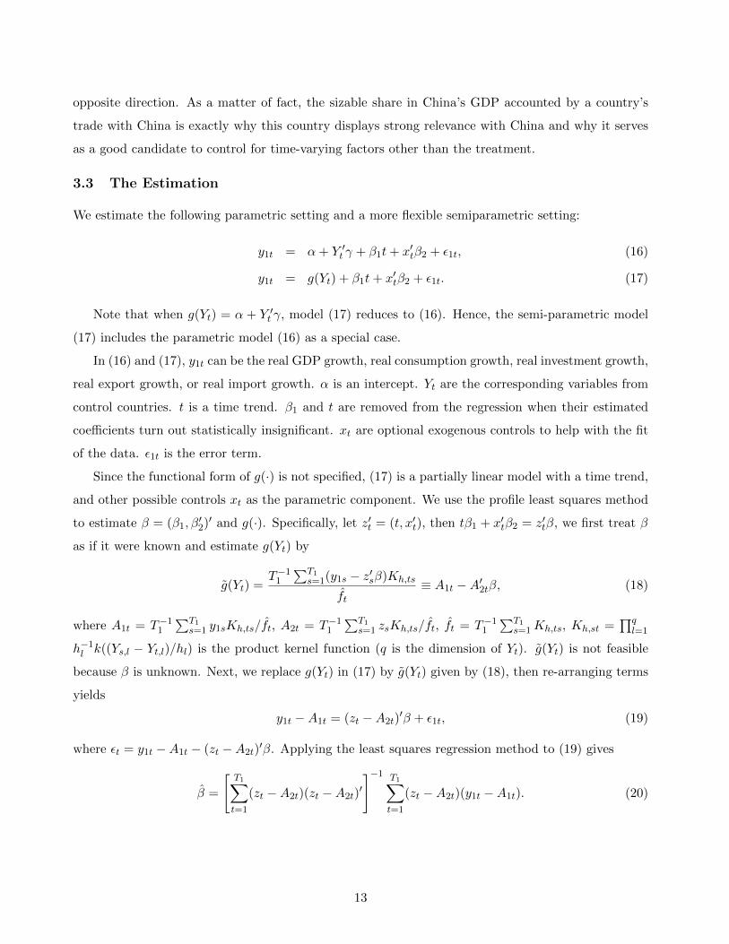
To predict the post-treatment counterfactuals for China, we apply the estimated coefficients to
the post-treatment data of the control countries. Figure 1 plots, starting from the fourth quarter of
2008 until the first quarter of 2013, the values of the predicted counterfactuals based on the paramet-
ric estimation (the dashed line) and those based on the semi-parametric estimation (the dotted line)
together with the observed under-treatment data (the solid line). As Figure 1 shows, the dashed line
and the dotted line almost coincide over the entire sample period, implying the parametric estima-
tion results are very consistent with the semi-parametric estimation results and thus the parametric
model is correctly specified. The two hypothetical lines track the solid line quite closely before the
6Our search for good control countries suggests that most countries with relatively strong prediction powers for China’skey macro variables turn out to have short time series for available data. For example, Poland and Russian Republicdisplay strong prediction powers for many variables for China, but Poland’s data starts from the first quarter of 1996and Russian Republic’s data starts from the first quarter of 2003.
14
treatment, suggesting good fit by both estimation settings. Starting from the treatment quarter, the
two hypothetical lines separate from the solid line: the actual growth moves above the hypothetical
counterfactual growths, implying a positive treatment effect. Starting from the fourth quarter of 2010,
the hypothetical lines move close to the solid line and track it closely again, suggesting the treatment
effect was temporary.
The actual under-treatment data, the predicted values of counterfactuals, and the estimated treat-
ment effects are listed in Panel B of Table 3. Based on the parametric estimation, the treatment
effects remained positive starting from the beginning of the treatment and peaked to 5.44% in the
third quarter of 2009. However, based on the semi-parametric estimation, the treatment effect did
not become evident until the second quarter of 2009 – about two quarters after the actual treatment
took place. The semi-parametric estimation suggests the treatment effect peaked to 6.12% also in
the third quarter of 2009. Both estimations suggest that, starting from the fourth quarter of 2010,
the treatment effect dropped below zero and remained afterward within an approximated value range
between -1% and zero.
The summary statistics of treatment effects are listed at the bottom of Panel B. For two years
after the fiscal stimulus, the actual real GDP growth in China averages at 9.39%, the parametrically
estimated counterfactual in the absence of the stimulus is 6.19%, suggesting an average treatment
effect for either quarters of 3.20%; the semi-parametrically estimated counterfactual equals 6.93%,
suggesting an average treatment effect of 2.46%. After the fourth quarter of 2010, the estimated
treatment effect averages only -0.17% according to the parametric estimation and -0.33% according
to the semi-parametric estimation. As a comparison, the standard deviation of the pre-treatment real
GDP growth from the actual data is 0.96%. This suggests negligible treatment effects two years after
the implementation of the fiscal stimulus.
Several remarks should be made regarding the timing of the treatment effects. Our estimates
suggest that, in the absence of the stimulus, the Chinese real GDP growth should have continued to
fall during the global financial crisis, reaching its bottom value of 2% or 3% around the third quarter of
2009. Our estimation suggests the policy intervention made the recovery two years earlier. Moreover,
although the program was implemented through 2010 only, there is no reason to believe its influence
cannot last past 2010. However, our estimates suggest its impact is indeed temporary. The real GDP
growth after 2010 would have been about the same even without the stimulus.
15
3.3.2 The Real GDP Components
As a further step, we examine the treatment effects on private components of real GDP: investment,
consumption, export, and import. Unfortunately, the semi-parametric estimation is not applicable here
as the available sample sizes for these variables in China are very small. Nonetheless, our estimation
results on the real GDP growth have already indicated that the parametric model is correctly specified
as the semi-parametric estimation produces very similar results to those of the parametric estimation.
Therefore, here we estimate the treatment effects on real investment growth, real consumption growth,
real export growth, and real import growth parametrically only, at the purpose of providing further
insights on how the stimulus package has influenced China’s macro economy.
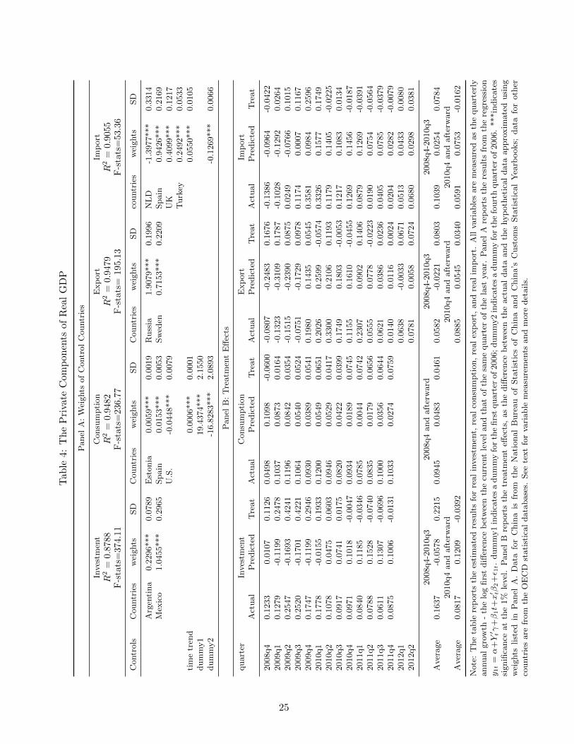
Panel A of Table 4 presents the estimated weights based on the pre-treatment data. The control
countries are Argentina and Mexico for investment, Estonia, Spain, and United States for consumption,
Russia and Sweden for export, and Netherlands, Spain, Turkey, and United Kingdom for import. All
these countries’ total trade volume with China over their own GDP ratios are below 5% according to
Table 2, implying the exogeneity criterion of our approach is satisfied. Panel A shows the adjusted
R2’s and F-statistics are all high, suggesting the related data series in the control countries are highly
correlated with the corresponding variables in China; hence, the relevance criterion is also met.
Figure 2 plots the actual and hypothetical series on real investment growth, real consumption
growth, real export growth, and real import growth before and after the treatment; the corresponding
data series are presented in Panel B of Table 4. The estimated results on the treatment effects can be
summarized as follows:
Firstly, the treatment effects are estimated to be all positive, but magnitudes of the responses
differ. The left column of Figure 2 shows the hypothetical series track the actual data quite well
before the treatment, but move below the actual data series after the treatment. In particular, we
estimate the stimulus package had raised China’s real investment growth by 22.15% , real consumption
growth by 4.61%, real export growth by 8.03%, and real import growth by 7.84%. In short, the 2008
Economic Stimulus Package had raised all private components of China’s real GDP.
Secondly, we estimate the treatment effects of the stimulus package to be temporary on all variables
except for consumption. The hypothetical series move close to the actual data series again, starting
from the fourth quarter of 2010 or slightly before. This suggests the package had raised China’s
investment, export, and import only temporarily. However, the hypothetical consumption growth
stays below the actual consumption growth throughout the entire sample period.
Thirdly, the timing of the responses to the stimulus package differs. As Figure 2 shows, investment
and export responded slightly before the actual taking place of the stimulus package, while consump-
16
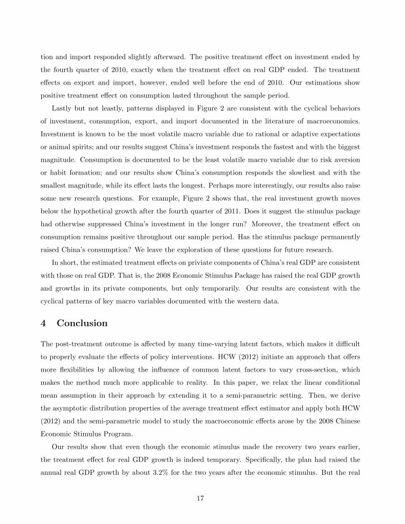
tion and import responded slightly afterward. The positive treatment effect on investment ended by
the fourth quarter of 2010, exactly when the treatment effect on real GDP ended. The treatment
effects on export and import, however, ended well before the end of 2010. Our estimations show
positive treatment effect on consumption lasted throughout the sample period.
Lastly but not leastly, patterns displayed in Figure 2 are consistent with the cyclical behaviors
of investment, consumption, export, and import documented in the literature of macroeconomics.
Investment is known to be the most volatile macro variable due to rational or adaptive expectations
or animal spirits; and our results suggest China’s investment responds the fastest and with the biggest
magnitude. Consumption is documented to be the least volatile macro variable due to risk aversion
or habit formation; and our results show China’s consumption responds the slowliest and with the
smallest magnitude, while its effect lasts the longest. Perhaps more interestingly, our results also raise
some new research questions. For example, Figure 2 shows that, the real investment growth moves
below the hypothetical growth after the fourth quarter of 2011. Does it suggest the stimulus package
had otherwise suppressed China’s investment in the longer run? Moreover, the treatment effect on
consumption remains positive throughout our sample period. Has the stimulus package permanently
raised China’s consumption? We leave the exploration of these questions for future research.
In short, the estimated treatment effects on priviate components of China’s real GDP are consistent
with those on real GDP. That is, the 2008 Economic Stimulus Package has raised the real GDP growth
and growths in its private components, but only temporarily. Our results are consistent with the
cyclical patterns of key macro variables documented with the western data.
4 Conclusion
The post-treatment outcome is affected by many time-varying latent factors, which makes it difficult
to properly evaluate the effects of policy interventions. HCW (2012) initiate an approach that offers
more flexibilities by allowing the influence of common latent factors to vary cross-section, which
makes the method much more applicable to reality. In this paper, we relax the linear conditional
mean assumption in their approach by extending it to a semi-parametric setting. Then, we derive
the asymptotic distribution properties of the average treatment effect estimator and apply both HCW
(2012) and the semi-parametric model to study the macroeconomic effects arose by the 2008 Chinese
Economic Stimulus Program.
Our results show that even though the economic stimulus made the recovery two years earlier,
the treatment effect for real GDP growth is indeed temporary. Specifically, the plan had raised the
annual real GDP growth by about 3.2% for the two years after the economic stimulus. But the real
17

GDP growth after 2010 would have been about the same without the stimulus. These results remain
robust to linear setting, semi-parametric setting and various control group selctions. Moreover, this
temporary boost is consistent with real investment growth, real consumption growth, real export
growth and real import growth.
18

References
Abadie, A., and Gardeazabal, J. (2003). The Economic Costs of Conflict: A Case Study of the Basque
Country. American Economic Review 93, 112-132.
Abadie, A., Diamond A. and Hainmueller J. (2010). Synthetic Control Methods for Comparative Case
Studies: Estimating the Effect of California’s Tobacco Control Program. Journal of the American
Statistical Association 105, 493-505.
Bai, J, and Ng S. (2002). Determining the number of factors in approximate factor models. Econo-
metrica 70, 191-221.
Bai, C., Li, Q. and Ouyang, M. (2014). Property Taxes and Home Prices: A Tale of Two Cities.
Journal of Econometrics, forthcoming.
Carroll, C., Slacalek, J. and Sommer, M. (2011). International evidence on sticky consumption growth.
Review of Economics and Statistics 93, 1135-1145.
Card, D. and Krueger, A.B. (1994). Minimum Wages and Employment: A Case Study of the Fast-Food
Industry in New Jersey and Pennsylvania. American Economic Review 84 (4): 772-793.
Ching, H.S., Hsiao, C. and Wan, S.K. (2012). Impact of CEPA on the labor market of Hong Kong.
China Economics Reviews 23, 975-981.
Fan, Y. and Li, Q. (1999). Root-n-consistent estimation of partially linear time series models. Journal
of Nonparametric Statistics 11, 251-269.
Hsiao, C., Ching, H.S. and Wand, S.K. (2012). A panel data approach for program evaluaton: Mea-
suring the benefit of political and economic integration of Hong Kong with mainland China. Journal
of Applied Econometrics 27(5), 705-740.
Robinson, P. (1988). Root-n-consistent semiparametric regression. Econometrica 56, 931-954.
Wong, C. (2011). The economic stimulus Program and Problems of Macroeconomic Management in
China. Handouts on the 32nd Annual Meeting of OECD Senior Budget Officials.
Yoshihara, K. (1976). Limiting behavior of U-statistic for stationary, absolutely regular processes. Z.
Wahrscheinlichkeistheorie verw. Gebiete 35, 237-252.
19
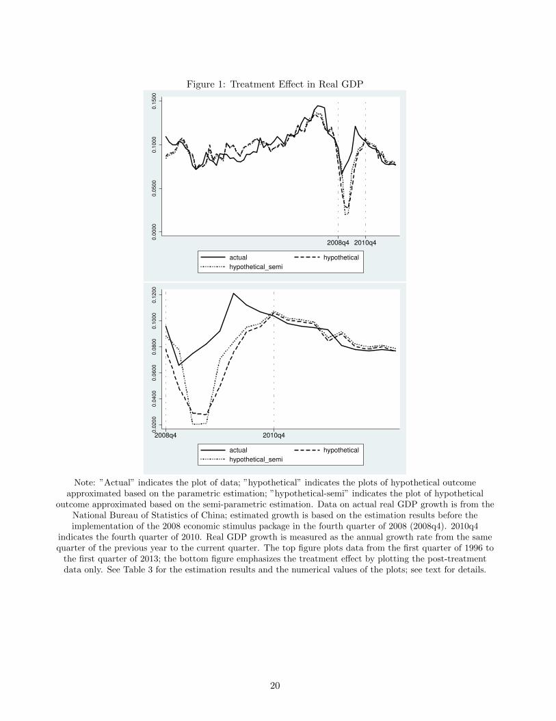
Figure 1: Treatment Effect in Real GDP
0.0
000
0.0
500
0.1
000
0.1
500
2008q4 2010q4
actual hypothetical
hypothetical_semi
0.0
200
0.0
400
0.0
600
0.0
800
0.1
000
0.1
200
2008q4 2010q4
actual hypothetical
hypothetical_semi
Note: ”Actual” indicates the plot of data; ”hypothetical” indicates the plots of hypothetical outcomeapproximated based on the parametric estimation; ”hypothetical-semi” indicates the plot of hypothetical
outcome approximated based on the semi-parametric estimation. Data on actual real GDP growth is from theNational Bureau of Statistics of China; estimated growth is based on the estimation results before theimplementation of the 2008 economic stimulus package in the fourth quarter of 2008 (2008q4). 2010q4
indicates the fourth quarter of 2010. Real GDP growth is measured as the annual growth rate from the samequarter of the previous year to the current quarter. The top figure plots data from the first quarter of 1996 to
the first quarter of 2013; the bottom figure emphasizes the treatment effect by plotting the post-treatmentdata only. See Table 3 for the estimation results and the numerical values of the plots; see text for details.
20
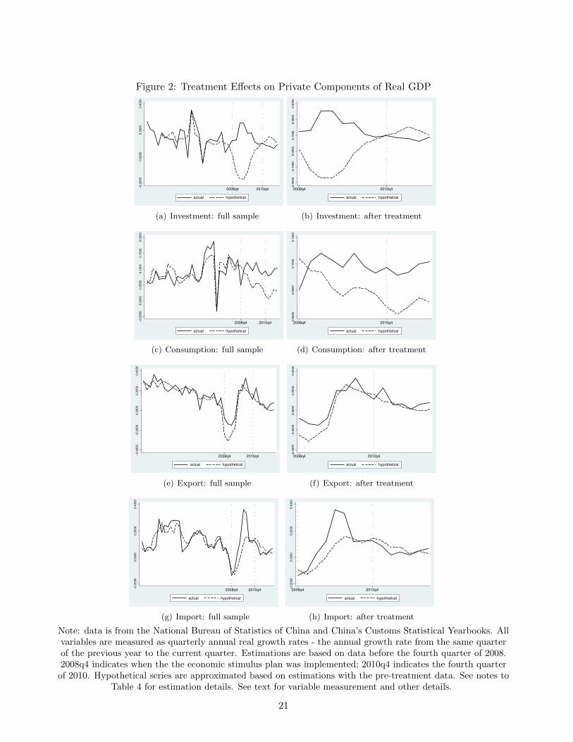
Figure 2: Treatment Effects on Private Components of Real GDP
−0.2
000
0.0
000
0.2
000
0.4
000
2008q4 2010q4
actual hypothetical
(a) Investment: full sample
−0.2
000
−0.1
000
0.0
000
0.1
000
0.2
000
0.3
000
2008q4 2010q4
actual hypothetical
(b) Investment: after treatment
−0.0
500
0.0
000
0.0
500
0.1
000
0.1
500
0.2
000
2008q4 2010q4
actual hypothetical
(c) Consumption: full sample
0.0
000
0.0
500
0.1
000
0.1
500
2008q4 2010q4
actual hypothetical
(d) Consumption: after treatment
−0.4
000
−0.2
000
0.0
000
0.2
000
0.4
000
2008q4 2010q4
actual hypothetical
(e) Export: full sample
−0.4
000
−0.2
000
0.0
000
0.2
000
0.4
000
2008q4 2010q4
actual hypothetical
(f) Export: after treatment
−0.2
000
0.0
000
0.2
000
0.4
000
2008q4 2010q4
actual hypothetical
(g) Import: full sample
−0.2
000
0.0
000
0.2
000
0.4
000
2008q4 2010q4
actual hypothetical
(h) Import: after treatment
Note: data is from the National Bureau of Statistics of China and China’s Customs Statistical Yearbooks. Allvariables are measured as quarterly annual real growth rates - the annual growth rate from the same quarterof the previous year to the current quarter. Estimations are based on data before the fourth quarter of 2008.2008q4 indicates when the the economic stimulus plan was implemented; 2010q4 indicates the fourth quarter
of 2010. Hypothetical series are approximated based on estimations with the pre-treatment data. See notes toTable 4 for estimation details. See text for variable measurement and other details.
21

Table 1: The Augmented Dickey-Fuller Tests Results
Countries GDP Investment Consumption Export Import
Argentina 0.0323 0.0022 0.0117 0.0170 0.0003Australia 0.0000 0.0000 0.0046 0.0036 0.0000Austria 0.1715 0.0189 0.6859 0.0046 0.0003Belgium 0.0009 0.0188 0.0118 0.0011 0.0005Brazil 0.0001 0.0016 0.0266 0.0717 0.0002Canada 0.0030 0.0001 0.0071 0.0088 0.0000Chile 0.4241 0.0189 0.0153 0.4795 0.0017Czech Republic 0.2390 0.0527 0.4041 0.0039 0.0020Denmark 0.0233 0.0935 0.0274 0.0081 0.0017Estonia 0.0286 0.2941 0.0068 0.0000 0.0026Finland 0.0069 0.0988 0.0600 0.0003 0.0001France 0.0013 0.0010 0.1948 0.0000 0.0000Germany 0.0004 0.0054 0.1573 0.0023 0.0053Hungary 0.0052 0.0062 0.2041 0.0006 0.0010Iceland 0.3766 0.3787 0.0072 0.2609 0.1483India 0.2366 0.2465 0.2856 0.0262 0.0005Indonesia 0.0171 0.0064 0.0252 0.0000 0.0004Ireland 0.5846 0.7972 0.3765 0.0143 0.0636Israel 0.0037 0.2681 0.0247 0.0001 0.0058Italy 0.0008 0.0121 0.0011 0.0002 0.0000Japan 0.0006 0.0280 0.0083 0.0000 0.0073Korea 0.0000 0.0005 0.0003 0.0000 0.0000Luxembourg 0.0480 0.0032 0.0079 0.0006 0.0008Mexico 0.0014 0.0465 0.1835 0.1263 0.0817Netherlands 0.0142 0.1078 0.3549 0.0001 0.0023New Zealand 0.0001 0.0419 0.0215 0.0004 0.0031Norway 0.0045 0.0248 0.0122 0.0032 0.0163Poland 0.1625 0.6260 0.2779 0.0281 0.0090Portugal 0.0334 0.1306 0.0491 0.0030 0.0051Russian Federation 0.1636 0.2786 0.1249 0.0709 0.0976Slovak Republic 0.2701 0.0156 0.2740 0.0122 0.0059Slovenia 0.0107 0.2721 0.4024 0.0013 0.0424South Africa 0.0041 0.0547 0.0167 0.0027 0.0344Spain 0.0508 0.2750 0.0829 0.0401 0.0539Sweden 0.0009 0.1210 0.0172 0.0001 0.0000Switzerland 0.0023 0.0004 0.0729 0.0095 0.0024Turkey 0.0070 0.0019 0.0266 0.0025 0.0014United Kingdom 0.0009 0.0879 0.0136 0.0013 0.0019United States 0.0045 0.0340 0.0726 0.0003 0.0010China 0.0164 0.0375 0.0174 0.0002 0.0002
Note: this table reports the Mackinnon approximated p values of the augmented Dickey-Fuller tests on quarterly series for 40 countries. All variables are in real terms andmeasured as annual growth (the log first difference between each quarter and the samequarter of the last year). Test specifications include a drift and two lags. The samplesizes range from 37 to 85 with an average of 75. See the text for details on pricedeflators, measurements, and data sources.
22

Table 2: Exogeneity Measure: Trade with China over GDP Ratio
Countries trade/GDP Countries trade/GDP
Argentina 0.0441 Australia 0.0567*Austria 0.0118 Belgium 0.0122Brazil 0.0324 Canada 0.0679*Chile 0.0966* Czech Republic 0.0288Denmark 0.0237 Estonia 0.0285Finland 0.0400 France 0.0138Germany 0.0317 Hungary 0.0485Iceland 0.0076 India 0.0424Indonesia 0.0618* Ireland 0.0270Israel 0.0300 Italy 0.0166Japan 0.0550* Korea 0.1998*Luxembourg 0.0703* Mexico 0.0161Netherlands 0.0488 New Zealand 0.0339Norway 0.0104 Poland 0.0197Portugal 0.0107 Russian Federation 0.0343Slovak Republic 0.0301 Slovenia 0.0201South Africa 0.0654* Spain 0.0165Sweden 0.0209 Switzerland 0.0215Turkey 0.0172 United Kingdom 0.0172United States 0.0235
Note: this table reports the total nominal trade volume with China as aratio of each country’s nominal GDP for the 39 sample OECD countries.Total trade volume is measured as the sum of nominal values of import andexport between the sample country and China. The reported ratios arethe average of 2008, 2009, and 2010. Data are from the Chinese CustomsYear Books of 2008, 2009, and 2010. *indicates that the ratio exceeds thethreshold value of 5% and violates the exogeneity criterion.
23
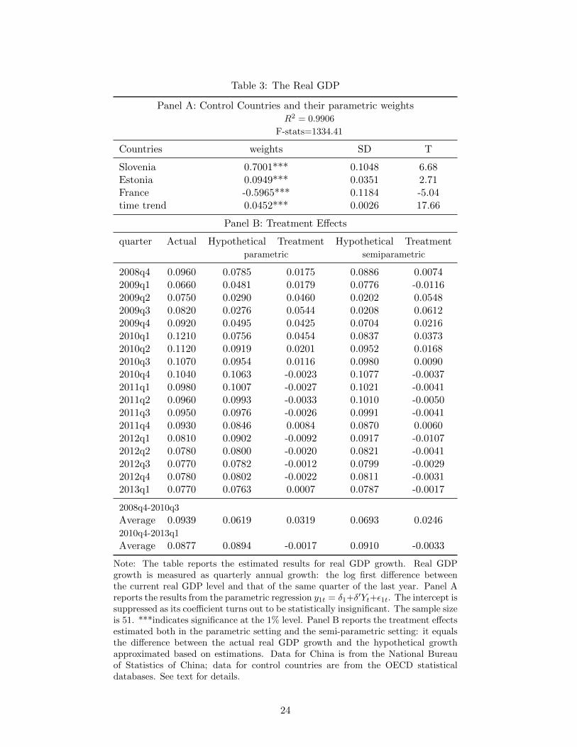
Table 3: The Real GDP
Panel A: Control Countries and their parametric weightsR2 = 0.9906
F-stats=1334.41
Countries weights SD T
Slovenia 0.7001*** 0.1048 6.68Estonia 0.0949*** 0.0351 2.71France -0.5965*** 0.1184 -5.04time trend 0.0452*** 0.0026 17.66
Panel B: Treatment Effects
quarter Actual Hypothetical Treatment Hypothetical Treatmentparametric semiparametric
2008q4 0.0960 0.0785 0.0175 0.0886 0.00742009q1 0.0660 0.0481 0.0179 0.0776 -0.01162009q2 0.0750 0.0290 0.0460 0.0202 0.05482009q3 0.0820 0.0276 0.0544 0.0208 0.06122009q4 0.0920 0.0495 0.0425 0.0704 0.02162010q1 0.1210 0.0756 0.0454 0.0837 0.03732010q2 0.1120 0.0919 0.0201 0.0952 0.01682010q3 0.1070 0.0954 0.0116 0.0980 0.00902010q4 0.1040 0.1063 -0.0023 0.1077 -0.00372011q1 0.0980 0.1007 -0.0027 0.1021 -0.00412011q2 0.0960 0.0993 -0.0033 0.1010 -0.00502011q3 0.0950 0.0976 -0.0026 0.0991 -0.00412011q4 0.0930 0.0846 0.0084 0.0870 0.00602012q1 0.0810 0.0902 -0.0092 0.0917 -0.01072012q2 0.0780 0.0800 -0.0020 0.0821 -0.00412012q3 0.0770 0.0782 -0.0012 0.0799 -0.00292012q4 0.0780 0.0802 -0.0022 0.0811 -0.00312013q1 0.0770 0.0763 0.0007 0.0787 -0.0017
2008q4-2010q3
Average 0.0939 0.0619 0.0319 0.0693 0.02462010q4-2013q1
Average 0.0877 0.0894 -0.0017 0.0910 -0.0033
Note: The table reports the estimated results for real GDP growth. Real GDPgrowth is measured as quarterly annual growth: the log first difference betweenthe current real GDP level and that of the same quarter of the last year. Panel Areports the results from the parametric regression y1t = δ1+δ′Yt+ε1t. The intercept issuppressed as its coefficient turns out to be statistically insignificant. The sample sizeis 51. ***indicates significance at the 1% level. Panel B reports the treatment effectsestimated both in the parametric setting and the semi-parametric setting: it equalsthe difference between the actual real GDP growth and the hypothetical growthapproximated based on estimations. Data for China is from the National Bureauof Statistics of China; data for control countries are from the OECD statisticaldatabases. See text for details.
24
Tab
le4:
Th
eP
riva
teC
omp
onen
tsof
Rea
lG
DP
Panel
A:
Wei
ghts
of
Contr
ol
Countr
ies
Inves
tmen
tC
onsu
mpti
on
Exp
ort
Imp
ort
R2
=0.
8788
R2
=0.
9482
R2
=0.
9479
R2
=0.
9055
F-s
tats
=37
4.11
F-s
tats
=236.7
7F
-sta
ts=
195.1
3F
-sta
ts=
53.3
6
Contr
ols
Countr
ies
wei
ghts
SD
Countr
ies
wei
ghts
SD
Countr
ies
wei
ghts
SD
countr
ies
wei
ghts
SD
Arg
enti
na
0.2
296***
0.0
789
Est
onia
0.0
059***
0.0
019
Russ
ia1.9
079***
0.1
996
NL
D-1
.3977***
0.3
314
Mex
ico
1.0
455***
0.2
965
Spain
0.0
153***
0.0
053
Sw
eden
0.7
153***
0.2
209
Spain
0.9
426***
0.2
169
U.S
.-0
.0448***
0.0
079
UK
0.4
099***
0.1
217
Turk
ey0.2
492***
0.0
533
tim
etr
end
0.0
006***
0.0
001
0.0
550***
0.0
105
dum
my1
19.4
374***
2.1
550
dum
my2
-16.8
283***
2.0
893
-0.1
269***
0.0
066
Panel
B:
Tre
atm
ent
Eff
ects
quart
erIn
ves
tmen
tC
onsu
mpti
on
Exp
ort
Imp
ort
Act
ual
Pre
dic
ted
Tre
at
Act
ual
Pre
dic
ted
Tre
at
Act
ual
Pre
dic
ted
Tre
at
Act
ual
Pre
dic
ted
Tre
at
2008q4
0.1
233
0.0
107
0.1
126
0.0
498
0.1
098
-0.0
600
-0.0
807
-0.2
483
0.1
676
-0.1
386
-0.0
964
-0.0
422
2009q1
0.1
279
-0.1
199
0.2
478
0.1
037
0.0
873
0.0
164
-0.1
323
-0.3
109
0.1
787
-0.1
028
-0.1
292
0.0
264
2009q2
0.2
547
-0.1
693
0.4
241
0.1
196
0.0
842
0.0
354
-0.1
515
-0.2
390
0.0
875
0.0
249
-0.0
766
0.1
015
2009q3
0.2
520
-0.1
701
0.4
221
0.1
064
0.0
540
0.0
524
-0.0
751
-0.1
729
0.0
978
0.1
174
0.0
007
0.1
167
2009q4
0.1
747
-0.1
199
0.2
946
0.0
930
0.0
389
0.0
541
0.1
980
0.1
435
0.0
545
0.3
581
0.0
984
0.2
596
2010q1
0.1
778
-0.0
155
0.1
933
0.1
200
0.0
549
0.0
651
0.2
026
0.2
599
-0.0
574
0.3
326
0.1
577
0.1
749
2010q2
0.1
078
0.0
475
0.0
603
0.0
946
0.0
529
0.0
417
0.3
300
0.2
106
0.1
193
0.1
179
0.1
405
-0.0
225
2010q3
0.0
917
0.0
741
0.0
175
0.0
820
0.0
422
0.0
399
0.1
749
0.1
803
-0.0
053
0.1
217
0.1
083
0.0
134
2010q4
0.0
971
0.1
018
-0.0
047
0.0
934
0.0
189
0.0
745
0.1
155
0.1
610
-0.0
455
0.1
269
0.1
456
-0.0
187
2011q1
0.0
840
0.1
185
-0.0
346
0.0
785
0.0
044
0.0
742
0.2
307
0.0
902
0.1
406
0.0
879
0.1
269
-0.0
391
2011q2
0.0
788
0.1
528
-0.0
740
0.0
835
0.0
179
0.0
656
0.0
555
0.0
778
-0.0
223
0.0
190
0.0
754
-0.0
564
2011q3
0.0
611
0.1
307
-0.0
696
0.1
000
0.0
356
0.0
644
0.0
621
0.0
386
0.0
236
0.0
405
0.0
785
-0.0
379
2011q4
0.0
875
0.1
006
-0.0
131
0.1
033
0.0
274
0.0
759
0.0
140
0.0
116
0.0
024
0.0
204
0.0
282
-0.0
079
2012q1
0.0
638
-0.0
033
0.0
671
0.0
513
0.0
433
0.0
080
2012q2
0.0
781
0.0
058
0.0
724
0.0
680
0.0
298
0.0
381
2008q4-2
010q3
2008q4
and
aft
erw
ard
2008q4-2
010q3
2008q4-2
010q3
Aver
age
0.1
637
-0.0
578
0.2
215
0.0
945
0.0
483
0.0
461
0.0
582
-0.0
221
0.0
803
0.1
039
0.0
254
0.0
784
2010q4
and
aft
erw
ard
2010q4
and
aft
erw
ard
2010q4
and
aft
erw
ard
Aver
age
0.0
817
0.1
209
-0.0
392
0.0
885
0.0
545
0.0
340
0.0
591
0.0
753
-0.0
162
Note
:T
he
table
rep
ort
sth
ees
tim
ate
dre
sult
sfo
rre
al
inves
tmen
t,re
al
consu
mpti
on,
real
exp
ort
,and
real
imp
ort
.A
llva
riable
sare
mea
sure
das
the
quart
erly
annual
gro
wth
-th
elo
gfirs
tdiff
eren
ceb
etw
een
the
curr
ent
level
and
that
of
the
sam
equart
erof
the
last
yea
r.P
anel
Are
port
sth
ere
sult
sfr
om
the
regre
ssio
ny1t
=α
+Y′ tγ
+β1t+x′ tβ
2+ε 1t.
dum
my1
indic
ate
sa
dum
my
for
the
firs
tquart
erof2006;dum
my2
indic
ate
sa
dum
my
for
the
fourt
hquart
erof2006.
***in
dic
ate
ssi
gnifi
cance
at
the
1%
level
.P
anel
Bre
port
sth
etr
eatm
ent
effec
ts,
as
the
diff
eren
ceb
etw
een
the
act
ual
data
and
the
hyp
oth
etic
al
data
appro
xim
ate
dusi
ng
wei
ghts
list
edin
Panel
A.
Data
for
Chin
ais
from
the
Nati
onal
Bure
au
of
Sta
tist
ics
of
Chin
aand
Chin
a’s
Cust
om
sSta
tist
ical
Yea
rbooks;
data
for
oth
erco
untr
ies
are
from
the
OE
CD
stati
stic
al
data
base
s.See
text
for
vari
able
mea
sure
men
tsand
more
det
ails.
25
5 Appendix
We first introduce some notations and define some quantities. We will use An = Bn + (s.o.) to denote
that Bn is the leading term of An, where (s.o.) denote terms having probability order smaller than
that of Bn. Define ξt = z1t − E(z1t|z2t), and note that y1it = y0
1t + ∆1t, y01t = z′1tβ + θ(z2t) + ε1t, and
y01t = z′1tβ + θ(z2t), where θ(z2t) is a feasible estimator of θ(z2t) and is defined in (23) below. Hence,
for t ≥ T + 1 + 1, we have
∆1t = y11t − y0
1t
= y1t − z′1tβ − θ(z2t)
= ∆1t − z′1t(β − β)− [θ(z2t)− θ(z2t)] + ε1t. (22)
From Robinson (1988) or Fan and Li (1999) we know that β − β = Op(T−1/21 ).
Let E(y1t|z2t) and E(z1t|z2t) denote the kernel estimators of E(y1t|z2t) and E(z1t|z2t), respectively.
Using θ(z2t) = E(y1t|z2t)− E(z1t|z2t)′β and y1t − z′1tβ = θ(z2t) + ε1t, we obtain
θ(z2t) = E(y1t|z2t)− E(z1t|z2t)′β
= E(y1t|z2t)− E(z1t|z2t)′β − E(z1t|z2t)
′(β − β)
= E(y1t − z′1tβ|z2t)− E(z1t|z2t)′(β − β)
= θ(z2t) + [θ(z2t)− θ(z2t)] + ε1t − E(z1t|z2t)′(β − β), (23)
where in the last equality above we added/subtracted θ(z2t), and we also used E[y1t − z′1tβ|z2t] =
E[θ(z2t) + ε1t|z2t] ≡ θ(z2t) + ε1t, respectively.
Combining (22) and (23), and noticing that E(z1t|z2t)′(β − β) = E(z1t|z2t)
′(β − β) + op(T−1/21 )
for any t ∈ {1, ..., n} by the uniform convergence result of E(z1t|z2t) − E(z1t|z2t) over the compact
set Sn. The use a trimming set Sn is also needed to trim data near the boundary of the support.
We trim sufficiently small intervals off the boundaries when the boundary of the support zt is known.
However, in practice the boundaries of zt are usually unknown. In this case, we sort the data to find
the sample minimums and maximums of zt. With sufficiently large sample size, such sample minimums
and maximums converge to the true boundaries of zt. Hence, we just trim sufficiently small intervals
of the sample boundaries when true boundaries of S are unknown. Specifically, let S = [az, bz] denote
the support of zt. When az, bz are unknown, we use az ≡ min1≤t≤n zt and bz ≡ max1≤t≤n zt to
estimate az and bz, respectively. It is well established that az − az = Op(n−1) and bz − bz = Op(n
−1)
(they are super-consistent estimates) The trimming set can be chosen as Sn = [az + δz, bz − δz], where
δz = δn,z → 0 as n→∞ and that h/δz = o(1).
26
Hence, we have, for any t ∈ {1, ..., n},
∆1t = ∆1t + [θt − θt] + [ε1t − ε1t]− ξ′t(β − β) + op(T−1/21 ), (24)
where θt = θt(z2t) and θt − θt(z2t). θt and ε1t are defined as follows
θt ≡ θ(z2t) = T−11
T1∑s=1
θ(z2s)Kh,ts/ft, (25)
ε1t = T−11
T1∑s=1
ε1sKh,ts/ft, (26)
where Kh,ts =∏qj=1 h
−1j k((z2t,j − z2s,j)/hj), z2t,j is the jth component of z2t, ft = T−1
1
∑T1s=1Kh,ts.
Consequently we have
∆1 − ∆1 =1
T2
T∑t=T1+1
[∆1t −∆1t
]
=1
T2
T∑t=T1+1
[θt − θt] +1
T2
T∑t=T1+1
[ε1t − ε1t]− E(z1|z2)′(β − β) + op(T−1/21 )
= A1n +A2n −A3n + op(T−1/21 ), (27)
where E(z1|z2) = T−12
∑Tt=T1+1E(z1t|z2t) = Op(1), A1n = T−1
2
∑Tt=T1+1[θt−θt], A2n = T−1
2
∑Tt=T1+1[ε1t−
ε1t] and A3n = E(z1|z2)′(β − β).
Proof of Proposition 2.1 (i)
Using 1/f(z2t) = 1/f(z2t) + (s.o.) uniformly in t ∈ {1, ..., n}, it is straightforward to show that
A1n = A1n,0 + (s.o.), where A1n,0 is the leading term of A1n and is defined by
A1n,0 =1
T1T2
T∑t=T1+1
T1∑s=1
(θ(z2t)− θ(z2s))Kh,ts/f(z2t).
Let (z1t, z2t) be an independent process with the same marginal distribution as (z1t, z2t). By
following the proof arguments as in Fan and Li (1999), i.e., using lemma 1 of Yoshihara (1976), one
can show that E(A1n,0) = E(A1n,0) + (s.o.) and V ar(A1n,0) = V ar(A1n,0) + (s.o.), where A1n,0 is
defined as in A1n,0 except that (z1t, z2t) are replaced by (z1t, z2t) wherever they occur. Then it is easy
27
to evaluate E(A1n,0) and V ar(A1n,0) as follows:
E(A1n,0) = E{E[(θ(z2t)− θ(z2s))Kh,ts|z2t]/f(z2t)}
= −(µ2/2)
q∑j=1
h2jE{[θjj(z2t)f(z2t) + θj(z2t)fj(z2t)]/f(z2t)}+Op(||h||3)
≡q∑j=1
h2jBj +Op(||h||3)
= O(||h||2), (28)
where Kh,ts is defined the same way as Kh,ts but with z2t and z2s replaced by z2t and z2s, µ2 =∫k(v)v2dv and Bj = −(µ2/2)E{[θjj(z2t)f(z2t) + θj(z2t)fj(z2t)]/f(z2t)}.
Also, it is easy to show that
V ar(A1n,0) =1
T 21 T
22
[(T1T
22 + T 2
1 T2)O(||h||2) + T1T2O((h1...hq)−1)]
= op(T−11 + T−1
2 ). (29)
Equations (28) and (29) imply that
A1n,0 =
q∑j=1
h2jBj + o(T
−1/21 + T
−1/22 ) (30)
since T2||h||6 = o(1).
Next, we consider A2n. Similarly to the above derivations one can easily obtain that A2n =
A2n,0 + (s.o.), where A2n,0 is the leading term of A2n and is defined by
A2n,0 =1
T2
T∑t=T1+1
[ε1t − ε1t]ft/ft
=1
T1T2
T∑t=T1+1
T1∑s=1
(ε1t − ε1s)Kh,ts/ft
=1
T1T2
T∑t=T1+1
T1∑s=1
HT1(w2t, w2s)
=1
T1
T1∑s=1
Hs +1
T2
T∑t=T1+1
Ht +1
T1T2
T1∑s=1
T∑t=T1+1
[Hts −Ht −Hs]
=1
T1
T1∑s=1
ε1t −1
T2
T∑t=T1+1
ε1s + op(max{T−1/21 , T
−1/22 })
= Op(T−1/21 + T
−1/22 ), (31)
28
where Hts = HT1(w2t, w2s) = (ε1t − ε1s)Kh,ts/ft, wt = (ε1t, z2t), Ht = E[Hts|z2t] = ε1t + (s.o.),
Hs = E[Hts|z2s] = −ε1s + (s.o.), and we also use the fact that the second moment of Bndef=
1T1T2
∑T1s=1
∑Tt=T1+1[Hts − Ht − Hs] is O((T1T2h1...hq)
−1) = o(max{T−11 , T−1
2 }), which implies that
Bn = op(max{T−1/21 , T
−1/22 }).
Finally, A3n = Op(T−1/21 ) follows from β − β = Op(T
−1/21 ) (e.g., Robinson (1988) or Fan and Li
(1999)). Summarizing the above we have shown that
∆1 − ∆1 = Op(||h||2 + T−1/21 + T
−1/22 ). (32)
Proof of Proposition 2.1 (ii)
By adding/subtracting ∆1 in (32) and using the fact that ∆1 −∆1 = Op(T−1/22 ), we obtain from
(32) that
∆1 −∆1 = ∆1 − ∆1 + ∆1 −∆1
= Op(||h||2 + T−1/21 + T
−1/22 ). (33)
Proof of Theorem 2.2
Proof of Theorem 2.2 (i)
Because V ar(A1n) = V ar(A1n,0)+(s.o.) = o(T−11 +T−1
2 ), the variance of A1n is negligible compared
with other terms. Hence, A1n affects the asymptotic distribution of ∆1 − ∆1 only through its mean:
E(A1n,0) =∑q
j=1Bjh2j +O(||h||3) as derived in (28). Hence, under the condition that T1||h||6 = o(1)
and T2||h||6 = o(1), we have
A1n,0 =
q∑j=1
Bjh2j + op(T
−1/21 + T
−1/22 ), (34)
where Bj = −(µ2/2)E{[θjj(z2t)f(z2t) + θj(z2t)fj(z2t)]/f(z2t)}.
From (31) we have that
A2n,0 =1
T1
T1∑s=1
ε1t −1
T2
T∑t=T1+1
ε1s + op(max{T−1/21 , T
−1/22 }). (35)
Case (i)
Under the assumption that T2/T1 → 0 as T1, T2 →∞, we have
A2n,0 = − 1
T2
T∑t=T1+1
ε1s + op(T−1/22 ), (36)
29

From β − β = Op(T−1/21 ) we have
A3n = Op(T−1/21 ) = op(T
−1/22 ). (37)
Summarizing (34), (36) and (37), we have shown that
√T2
∆1 − ∆1 −q∑j=1
Bjh2j
= − 1√T2
T∑t=T1+1
ε1t + op(1)d→ N(0, σ2
ε ), (38)
and
√T2
∆1 −∆1 −q∑j=1
Bjh2j
=√T2
∆1 − ∆1 + ∆1 −∆1 −q∑j=1
Bjh2j
=
1√T2
T∑t=T1+1
−ε1t + ∆1t −∆1 −q∑j=1
Bjh2j
d→ N(0, σ2
∆ + σ2ε ). (39)
Case (ii).
If T2/T1 → λ ∈ (0,∞), from (35) we obtain
√T2A2n,0 =
√T2
1
T1
T1∑s=1
ε1t −1
T2
T∑t=T1+1
ε1s
+ op(max{T−1/21 , T
−1/22 })
d→ N(0, σ2ε (1 + λ)). (40)
By Theorem 2.1 of Fan and Li (1999) we know that√T1(β − β)
d→ N(0, V0), (41)
where V0 = A−1BA−1 is the asymptotic variance of√T2(β − β) with A = E(ξtξ
′t), B = E[ε21tξtξ
′t] and
ξt = z1t − E(z1t|z2t).
Using (41) we have that√T2A3n =
√T2/T1E(ξ′t)
√T1(β − β) + op(1)
d→ N(0, λE(ξ′t)V0E(ξt))
≡ N(0, V3), (42)
where V3 = λE(ξ′t)V0E(ξt).
Given that ∆t and ε1t, t = T1 +1, ..., T are uncorrelated with the pre-treatment data, we have that
30
the leading terms of A1n, A2n are asymptotically independent with the leading term of A3n.
Summarizing (34), (40) and (42), we have
√T2
∆1 − ∆1 −q∑j=1
Bjh2j
d→ N(0, σ2ε (1 + λ) + V3). (43)
By assumption A6, we have √T2(∆1 −∆1)
d→ N(0, σ2∆), (44)
where σ2∆ = limT2→∞ V ar(T
−1/22
∑Tt=T1+1 ∆1t). Also, given that E(ε1t|∆t) = 0, we have from (43)
and (44) that
√T2
∆1 −∆1 −q∑j=1
Bjh2j
=√T2
∆1 − ∆1 + ∆1 −∆1 −q∑j=1
Bjh2j
d→ N(0, σ2
ε + σ2∆ + V3). (45)
This completes the proof of Theorem 2.2.
31


