Two-Dimensional Shape and Texture Quantification
Medical Image Processing-BM4300
120405P
Shashika Chamod Munasingha
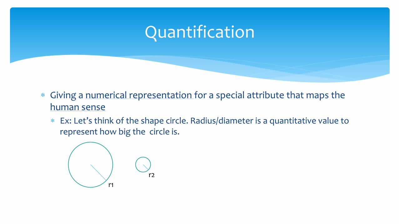
Giving a numerical representation for a special attribute that maps the human sense
Ex: Let’s think of the shape circle. Radius/diameter is a quantitative value to represent how big the circle is.
Quantification
r1
r2
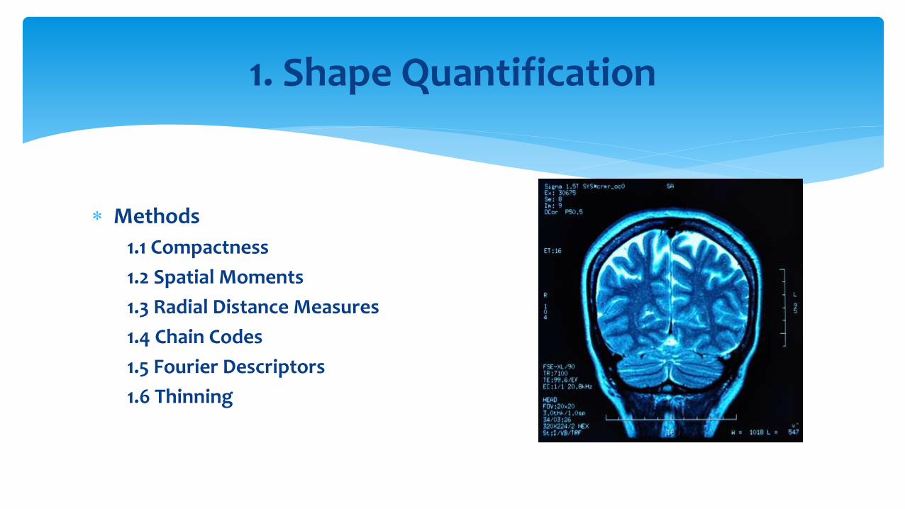
Methods
1.1 Compactness
1.2 Spatial Moments
1.3 Radial Distance Measures
1.4 Chain Codes
1.5 Fourier Descriptors
1.6 Thinning
1. Shape Quantification
Computed using the perimeter (P) and the area (A) of the segmented region
𝑪 = 𝑷𝟐/𝑨
Quantifies how close a shape is to the smoothest shape; circle
When the C is getting larger for a particular shape, it moves away from the shape circle.
Perfect circle has the smallest value for C
More details: ‘State of the Art of Compactness and Circularity Measures’ by Raul S. Montero
and Ernesto Bribiesca, 2009
1.1 Compactness (C)
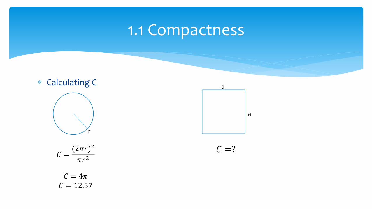
Calculating C
1.1 Compactness
𝐶 =(2𝜋𝑟)2
𝜋𝑟2
𝐶 = 4𝜋 𝐶 = 12.57
r
a
a
𝐶 =?
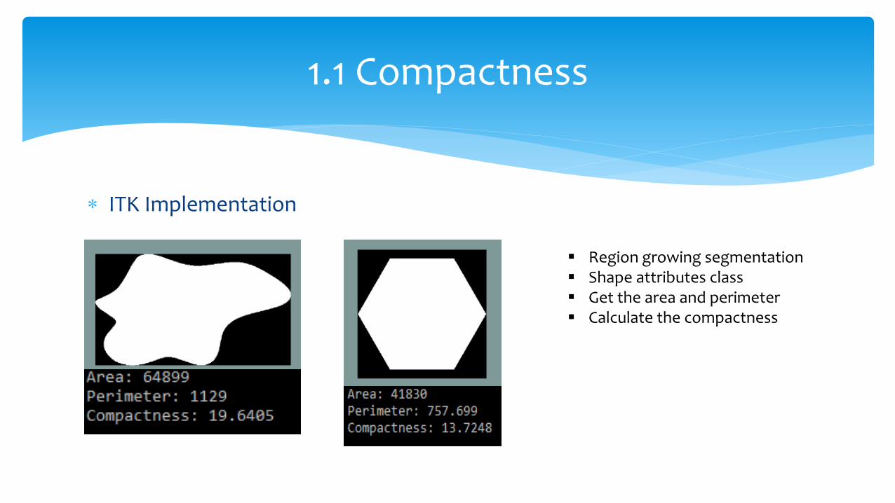
ITK Implementation
1.1 Compactness
Region growing segmentation Shape attributes class Get the area and perimeter Calculate the compactness
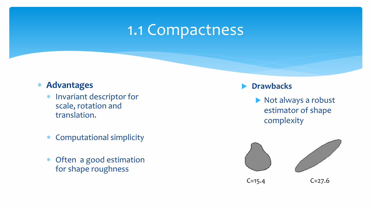
Advantages Invariant descriptor for
scale, rotation and translation.
Computational simplicity
Often a good estimation for shape roughness
1.1 Compactness
Drawbacks
Not always a robust estimator of shape complexity
C=15.4 C=27.6
Quantitative measurement of the distribution and the shape of set of points
A 2D digital image can be represented by 3 parameters (i ,j ,f ) ;
( i , j ) spatial coordinates and f( i, j ) be the intensity of pixels
More details : ‘Application of Shape Analysis to Mammographic Calcifications’ by Liang
Shen, Rangaraj M. Rangayyan, and J. E. Leo Desautels
1.2 Spatial Moments
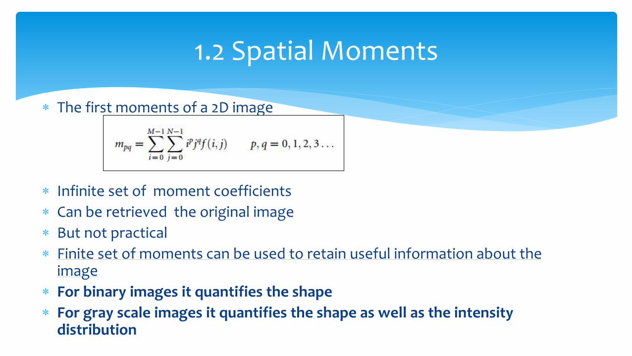
The first moments of a 2D image
Infinite set of moment coefficients
Can be retrieved the original image
But not practical
Finite set of moments can be used to retain useful information about the image
For binary images it quantifies the shape
For gray scale images it quantifies the shape as well as the intensity distribution
1.2 Spatial Moments
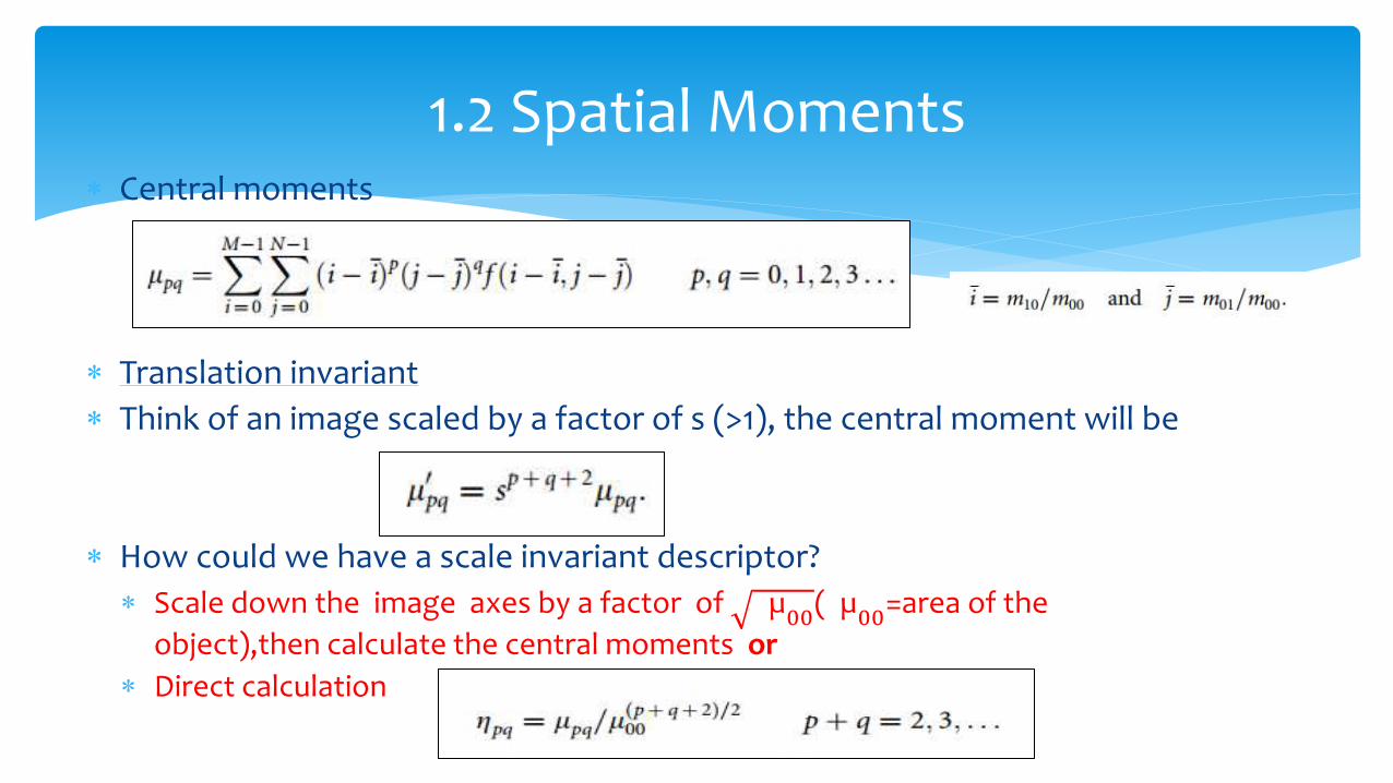
Central moments
Translation invariant
Think of an image scaled by a factor of s (>1), the central moment will be
How could we have a scale invariant descriptor?
Scale down the image axes by a factor of µ00
( µ00
=area of the
object),then calculate the central moments or
Direct calculation
1.2 Spatial Moments
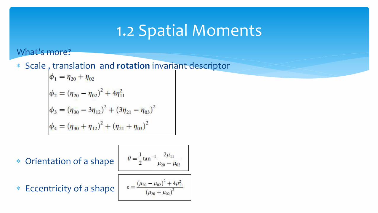
What's more?
Scale , translation and rotation invariant descriptor
Orientation of a shape
Eccentricity of a shape
1.2 Spatial Moments
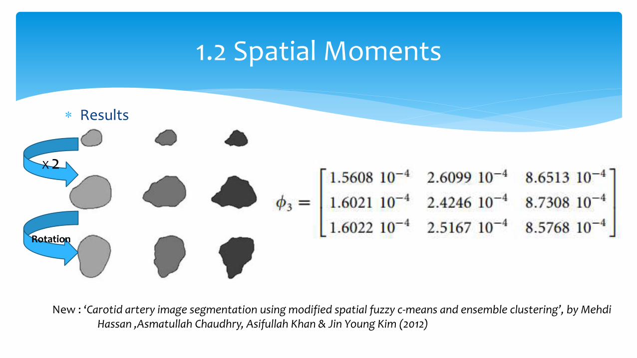
Results
1.2 Spatial Moments
X 2
Rotation
New : ‘Carotid artery image segmentation using modified spatial fuzzy c-means and ensemble clustering’, by Mehdi Hassan ,Asmatullah Chaudhry, Asifullah Khan & Jin Young Kim (2012)
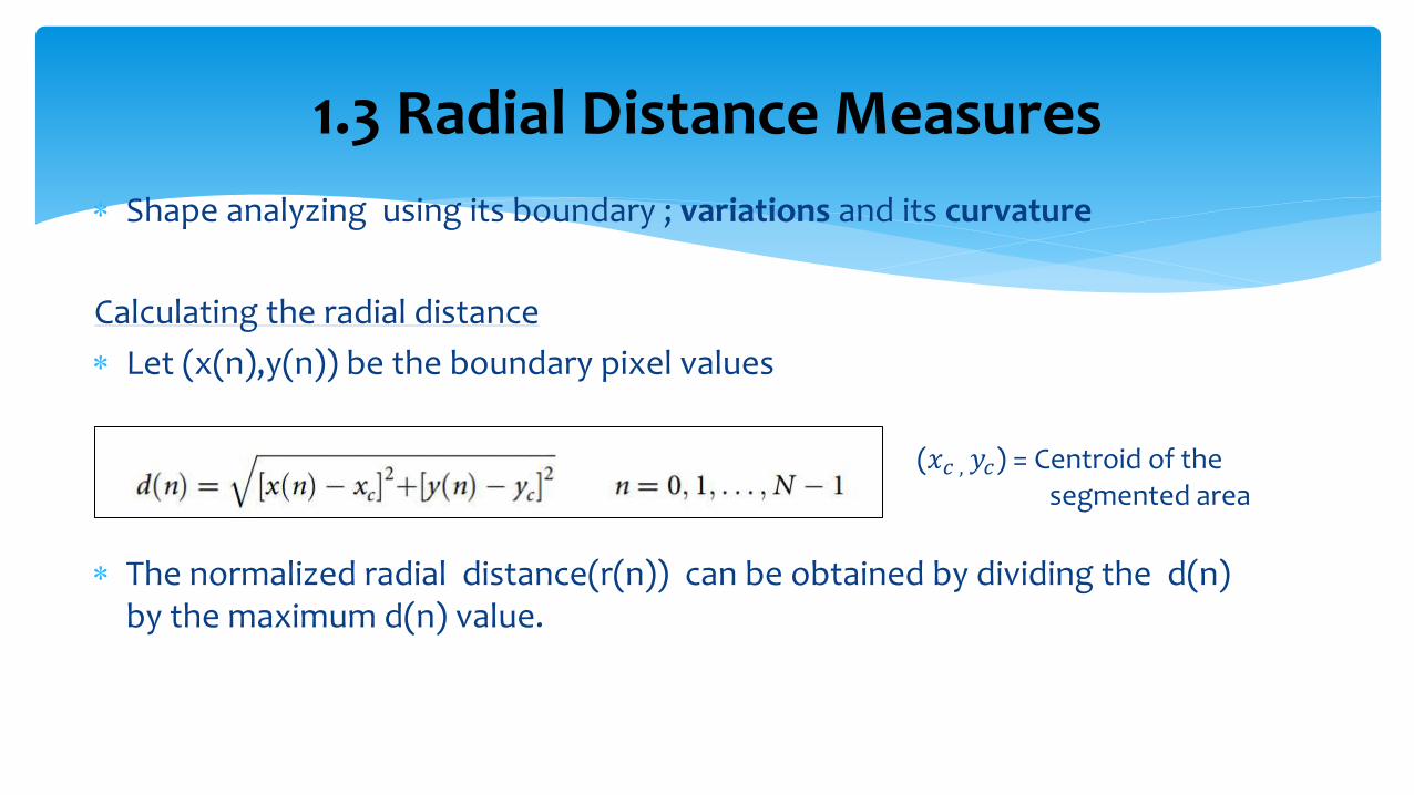
Shape analyzing using its boundary ; variations and its curvature
Calculating the radial distance
Let (x(n),y(n)) be the boundary pixel values
(𝑥𝑐 , 𝑦𝑐) = Centroid of the
segmented area
The normalized radial distance(r(n)) can be obtained by dividing the d(n) by the maximum d(n) value.
1.3 Radial Distance Measures
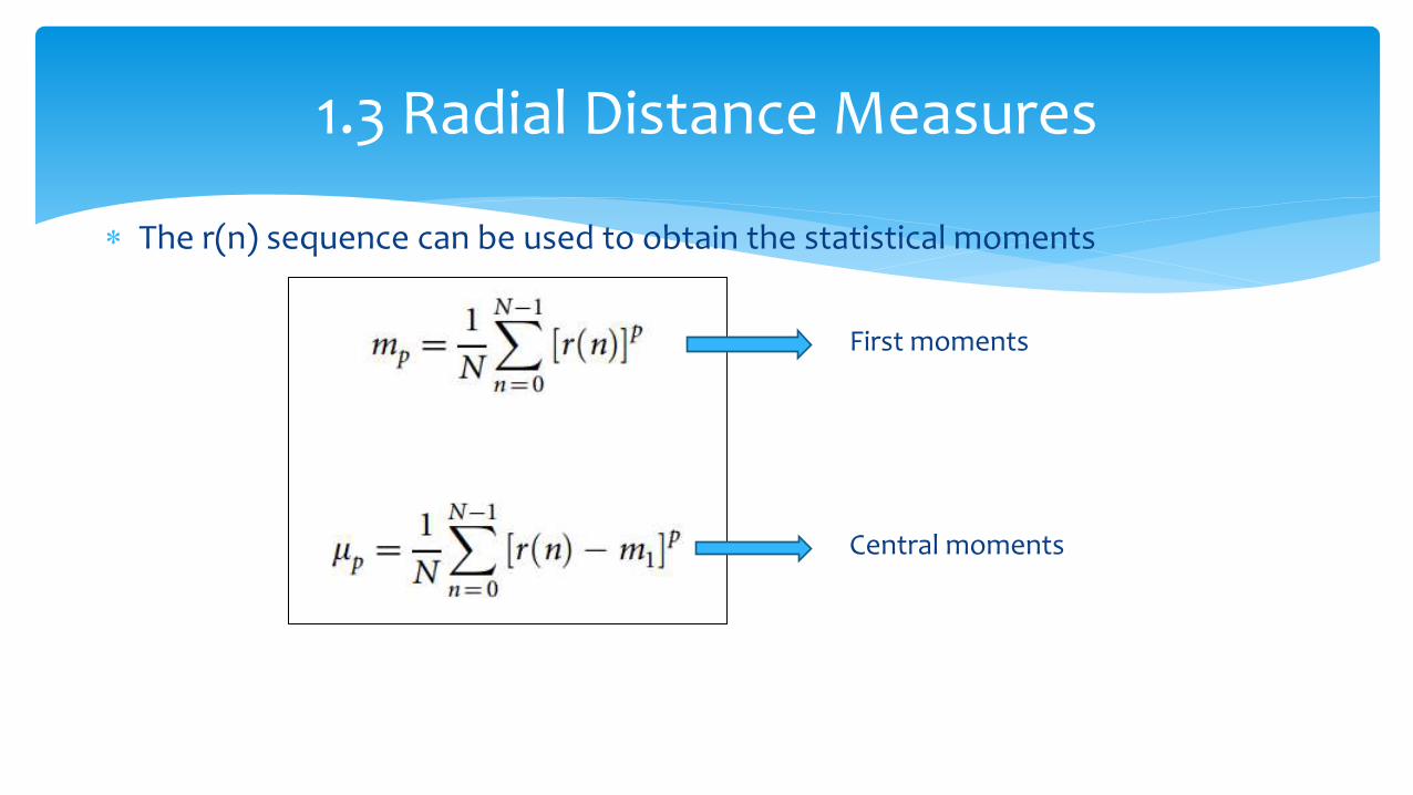
The r(n) sequence can be used to obtain the statistical moments
First moments
Central moments
1.3 Radial Distance Measures
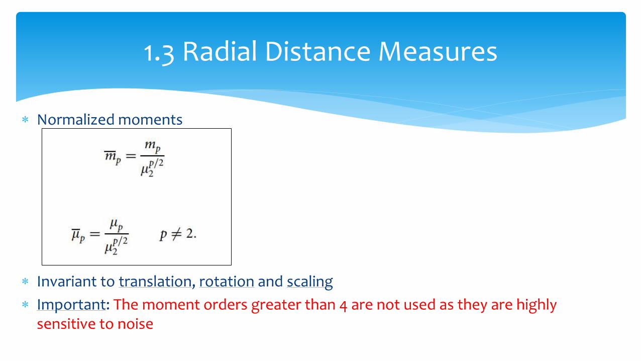
Normalized moments
Invariant to translation, rotation and scaling
Important: The moment orders greater than 4 are not used as they are highly sensitive to noise
1.3 Radial Distance Measures
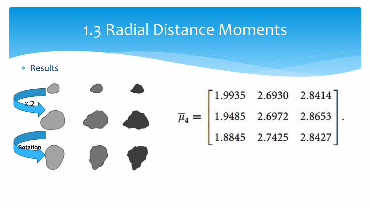
Results
1.3 Radial Distance Moments
X 2
Rotation
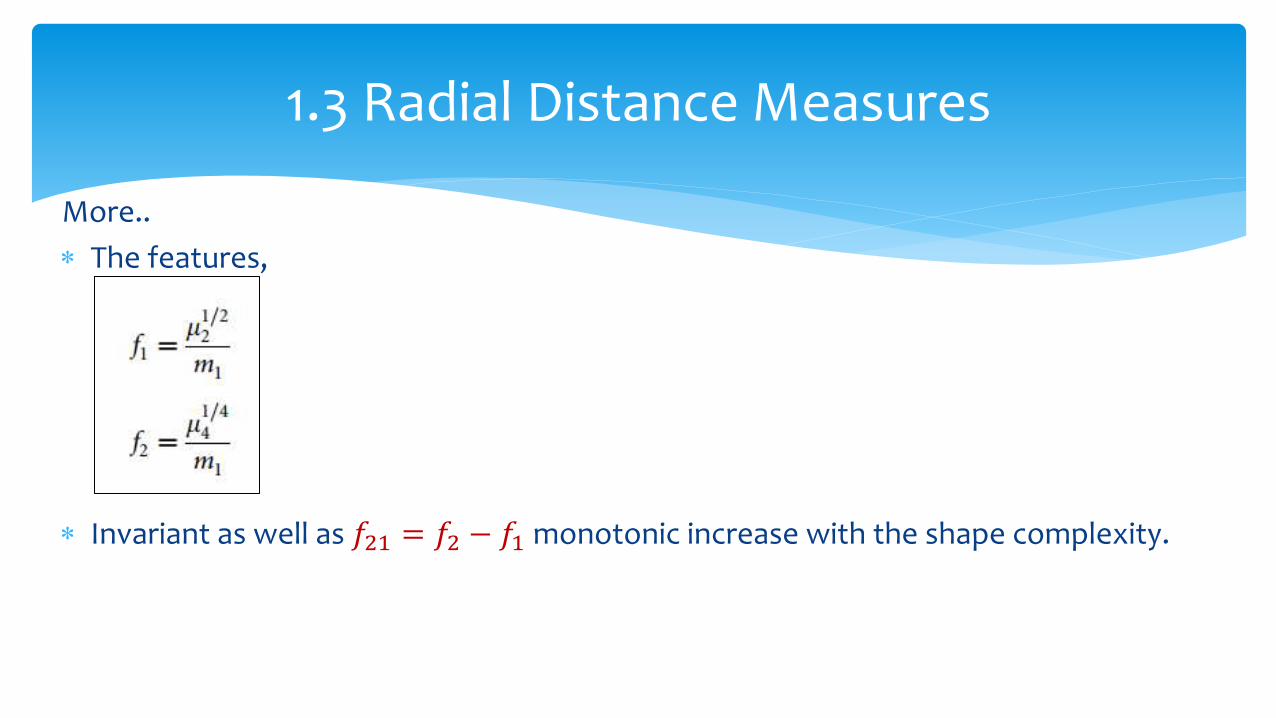
More..
The features,
Invariant as well as 𝑓21 = 𝑓2 − 𝑓1 monotonic increase with the shape complexity.
1.3 Radial Distance Measures
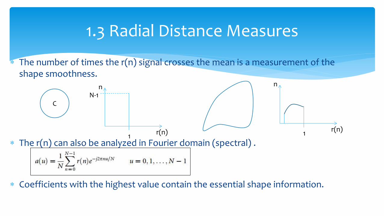
The number of times the r(n) signal crosses the mean is a measurement of the shape smoothness.
The r(n) can also be analyzed in Fourier domain (spectral) .
Coefficients with the highest value contain the essential shape information.
1.3 Radial Distance Measures
C
r(n) 1
N-1 n
r(n) 1
n
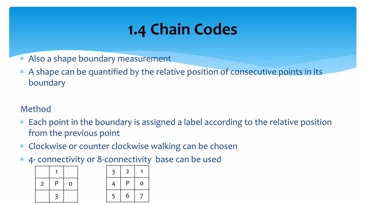
Also a shape boundary measurement
A shape can be quantified by the relative position of consecutive points in its boundary
Method
Each point in the boundary is assigned a label according to the relative position from the previous point
Clockwise or counter clockwise walking can be chosen
4- connectivity or 8-connectivity base can be used
1.4 Chain Codes
3 2 1
4 P 0
5 6 7
1
2 P 0
3
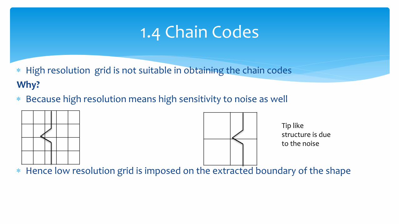
High resolution grid is not suitable in obtaining the chain codes
Why?
Because high resolution means high sensitivity to noise as well
Hence low resolution grid is imposed on the extracted boundary of the shape
1.4 Chain Codes
Tip like structure is due to the noise
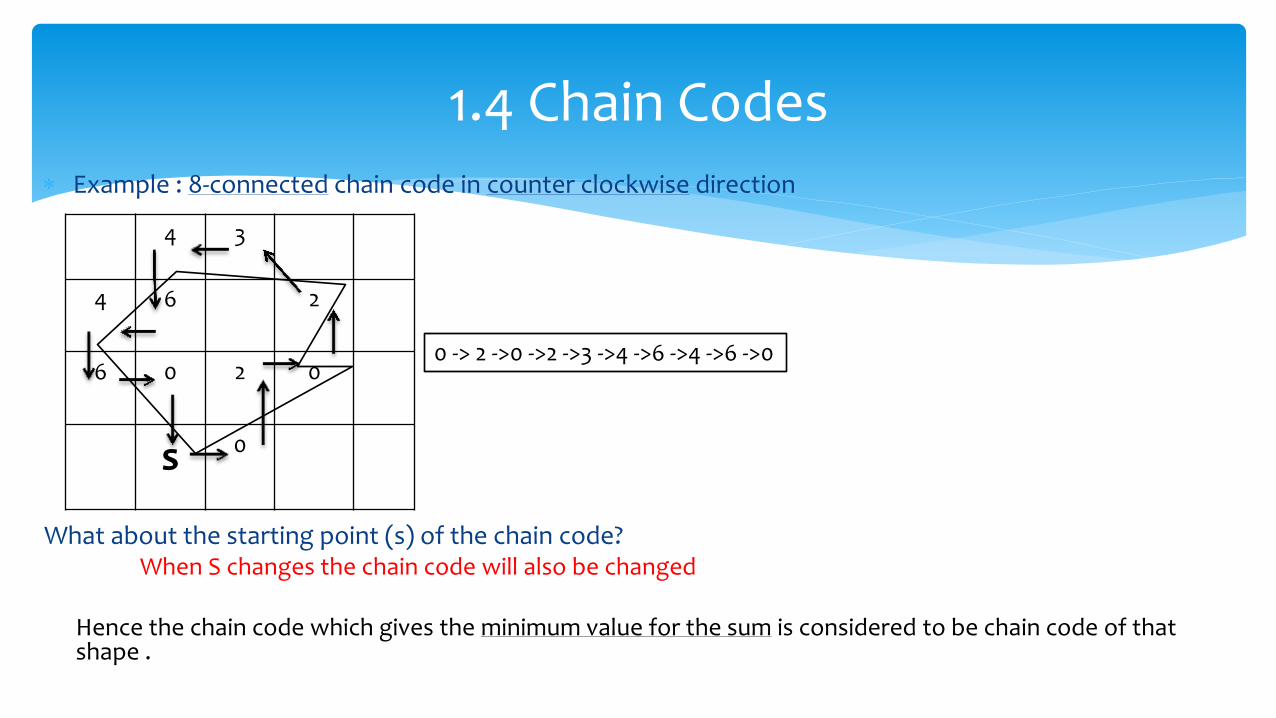
Example : 8-connected chain code in counter clockwise direction
What about the starting point (s) of the chain code? When S changes the chain code will also be changed Hence the chain code which gives the minimum value for the sum is considered to be chain code of that shape .
1.4 Chain Codes
4 3
4 6 2
6 0 2 0
s 0
0 -> 2 ->0 ->2 ->3 ->4 ->6 ->4 ->6 ->0
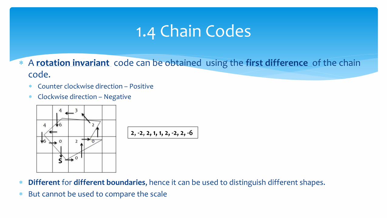
A rotation invariant code can be obtained using the first difference of the chain code. Counter clockwise direction – Positive
Clockwise direction – Negative
Different for different boundaries, hence it can be used to distinguish different shapes.
But cannot be used to compare the scale
1.4 Chain Codes
2, -2, 2, 1, 1, 2, -2, 2, -6
Is that all?
If the differential chain code shows very small values (0,1) over a local section of a boundary that section tends to be smoother.
If the shape is symmetric or nearly symmetric, the differential chain code will also have symmetric parts too.
Concave and Convex regions can also be identified using differential chain code Continuous positive differences – Convex region
Continuous negative differences – Concave region
New:
‘A measure of tortuosity based on chain coding’ by E Bribiesca - Pattern Recognition, 2013 – Elsevier
‘An automated lung segmentation approach using bidirectional chain codes to improve nodule detection accuracy’ by S Shen, AAT Bui, J Cong, W Hsu - Computers in biology and medicine, 2015 - Elsevier
1.4 Chain Codes

Each pixel on a selected contour can be represented by a complex number.
The DFT
Inverse DFT
Except the first coefficient d(0) in DFT (centroid), all other coefficients are translation invariant
Important information is on lower order coefficients of d(u)
1.5 Fourier Descriptors
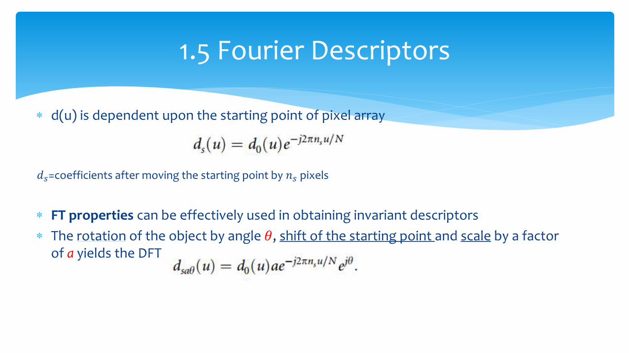
d(u) is dependent upon the starting point of pixel array
𝑑𝑠=coefficients after moving the starting point by 𝑛𝑠 pixels
FT properties can be effectively used in obtaining invariant descriptors
The rotation of the object by angle 𝜃, shift of the starting point and scale by a factor of a yields the DFT series
1.5 Fourier Descriptors
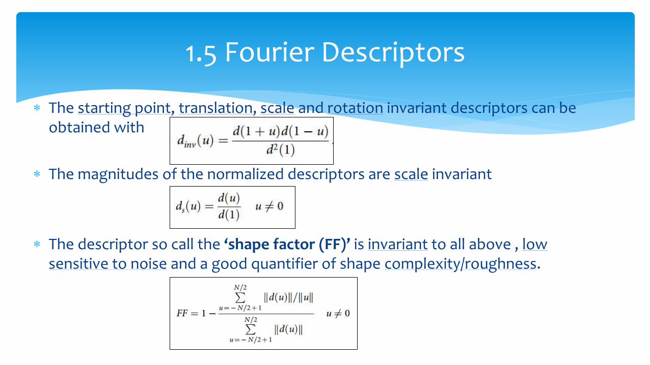
The starting point, translation, scale and rotation invariant descriptors can be obtained with
The magnitudes of the normalized descriptors are scale invariant
The descriptor so call the ‘shape factor (FF)’ is invariant to all above , low sensitive to noise and a good quantifier of shape complexity/roughness.
1.5 Fourier Descriptors
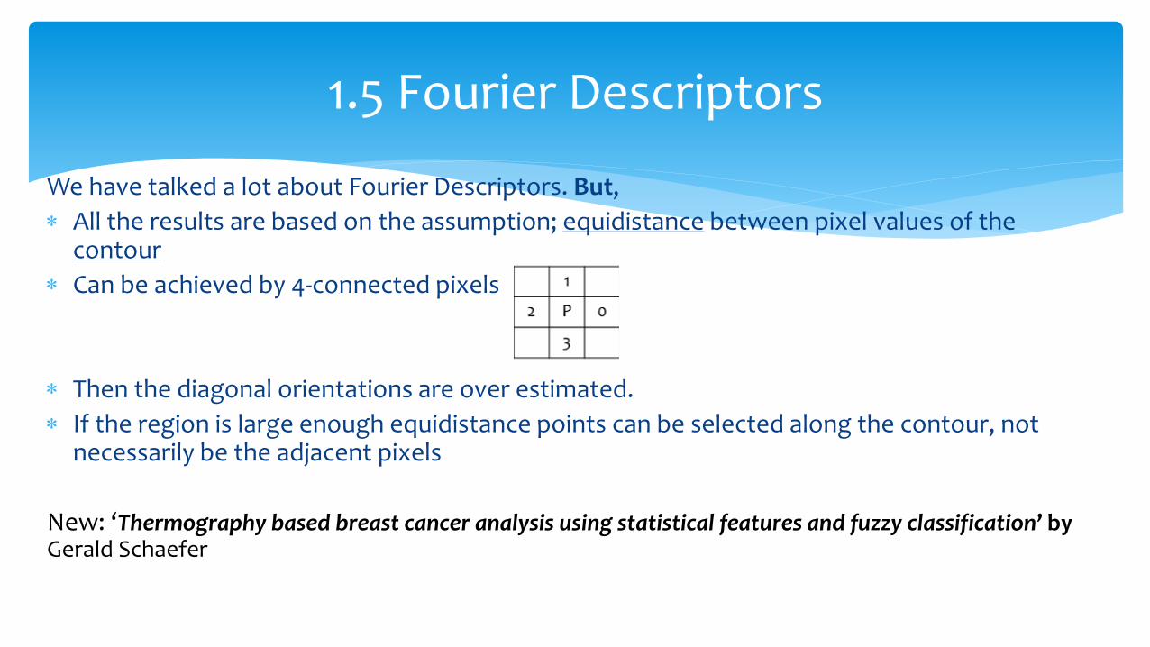
We have talked a lot about Fourier Descriptors. But,
All the results are based on the assumption; equidistance between pixel values of the contour
Can be achieved by 4-connected pixels
Then the diagonal orientations are over estimated.
If the region is large enough equidistance points can be selected along the contour, not necessarily be the adjacent pixels
New: ‘Thermography based breast cancer analysis using statistical features and fuzzy classification’ by Gerald Schaefer
1.5 Fourier Descriptors
The essential shape information can be represented by reducing the shape to a graph(skeleton)
Skeleton is made of the medial lines along the main shape
Medial lines are obtained via the medial axis transformation (MAT).
The computational complexity is high for the MAT algorithm.
Some iterative algorithms are introduced to reduce the computational complexity
Algorithm by Zhang and Suen is the widely used one among them
1.6 Thinning/Skeleton
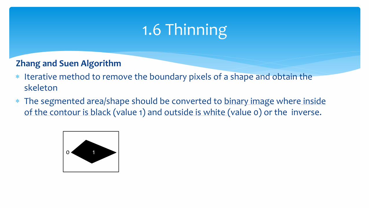
Zhang and Suen Algorithm
Iterative method to remove the boundary pixels of a shape and obtain the skeleton
The segmented area/shape should be converted to binary image where inside of the contour is black (value 1) and outside is white (value 0) or the inverse.
1.6 Thinning
0 1
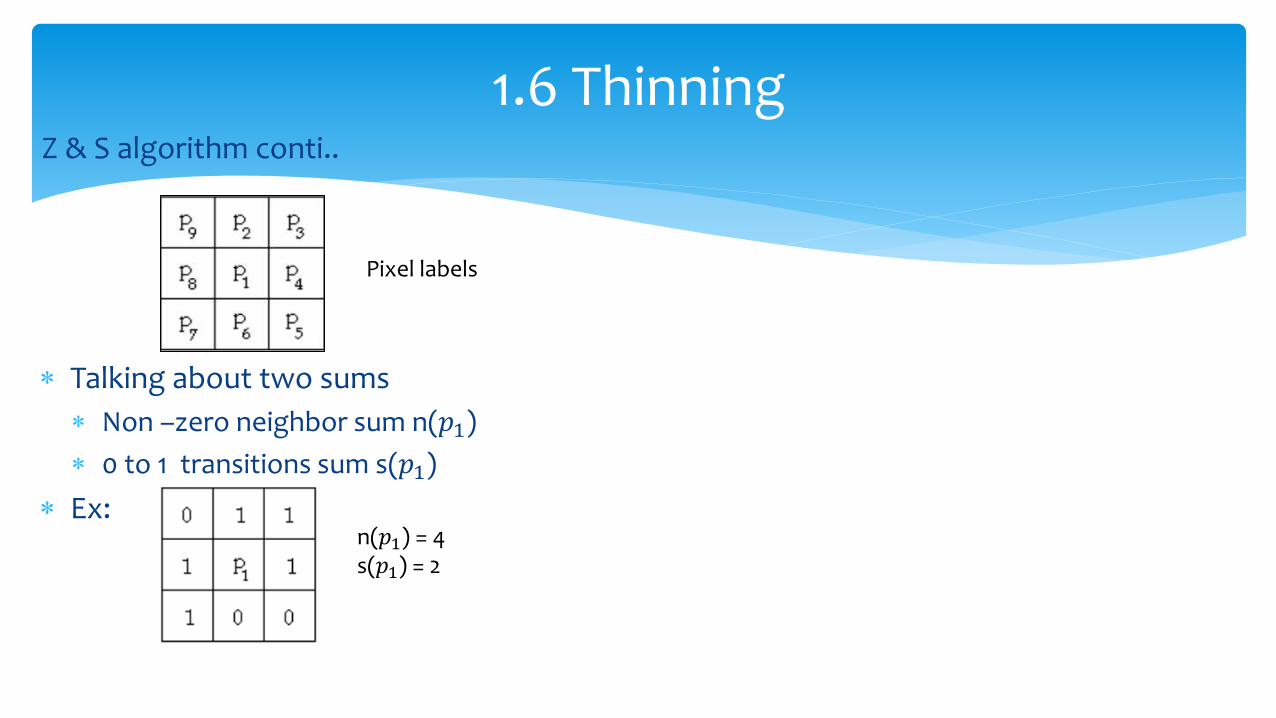
Z & S algorithm conti..
Talking about two sums
Non –zero neighbor sum n(𝑝1)
0 to 1 transitions sum s(𝑝1)
Ex:
1.6 Thinning
n(𝑝1) = 4 s(𝑝1) = 2
Pixel labels
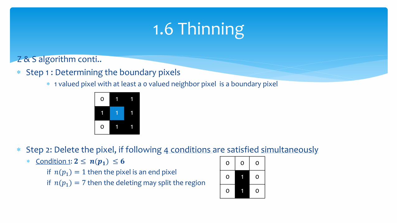
Z & S algorithm conti..
Step 1 : Determining the boundary pixels 1 valued pixel with at least a 0 valued neighbor pixel is a boundary pixel
Step 2: Delete the pixel, if following 4 conditions are satisfied simultaneously Condition 1: 𝟐 ≤ 𝒏(𝒑𝟏) ≤ 𝟔
if 𝑛(𝑝1) = 1 then the pixel is an end pixel
if 𝑛(𝑝1) = 7 then the deleting may split the region
1.6 Thinning
0 1 1
1 1 1
0 1 1
0 0 0
0 1 0
0 1 0
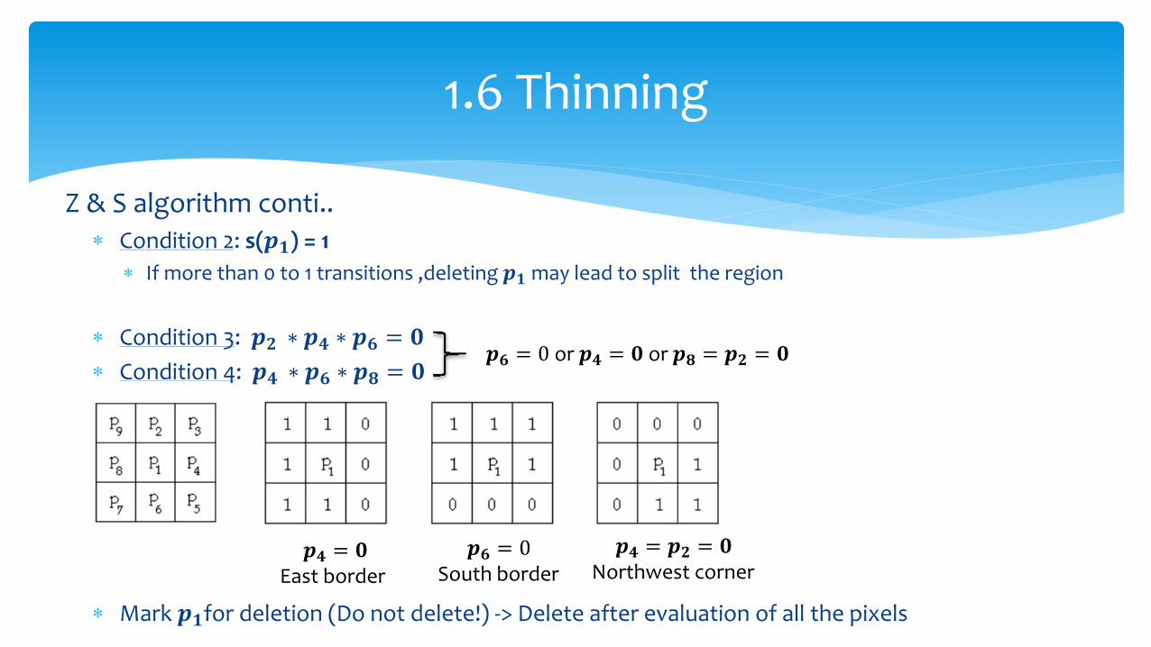
Z & S algorithm conti.. Condition 2: s(𝒑𝟏) = 1
If more than 0 to 1 transitions ,deleting 𝒑𝟏 may lead to split the region
Condition 3: 𝒑𝟐 ∗ 𝒑𝟒 ∗ 𝒑𝟔 = 𝟎
Condition 4: 𝒑𝟒 ∗ 𝒑𝟔 ∗ 𝒑𝟖 = 𝟎
Mark 𝒑𝟏for deletion (Do not delete!) -> Delete after evaluation of all the pixels
1.6 Thinning
𝒑𝟔 = 0 or 𝒑𝟒 = 𝟎 or 𝒑𝟖 = 𝒑𝟐 = 𝟎
𝒑𝟒 = 𝟎 East border
𝒑𝟔 = 0 South border
𝒑𝟒 = 𝒑𝟐 = 𝟎 Northwest corner
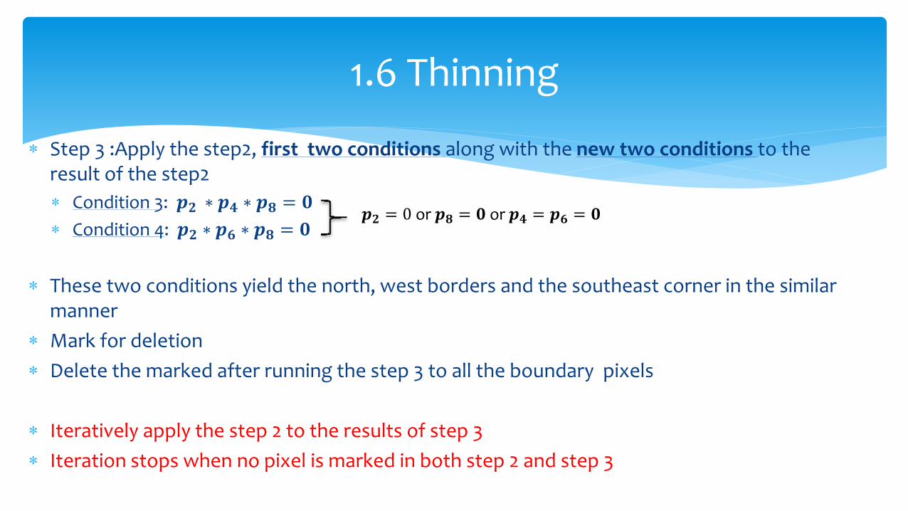
Step 3 :Apply the step2, first two conditions along with the new two conditions to the result of the step2
Condition 3: 𝒑𝟐 ∗ 𝒑𝟒 ∗ 𝒑𝟖 = 𝟎
Condition 4: 𝒑𝟐 ∗ 𝒑𝟔 ∗ 𝒑𝟖 = 𝟎
These two conditions yield the north, west borders and the southeast corner in the similar manner
Mark for deletion
Delete the marked after running the step 3 to all the boundary pixels
Iteratively apply the step 2 to the results of step 3
Iteration stops when no pixel is marked in both step 2 and step 3
1.6 Thinning
𝒑𝟐 = 0 or 𝒑𝟖 = 𝟎 or 𝒑𝟒 = 𝒑𝟔 = 𝟎
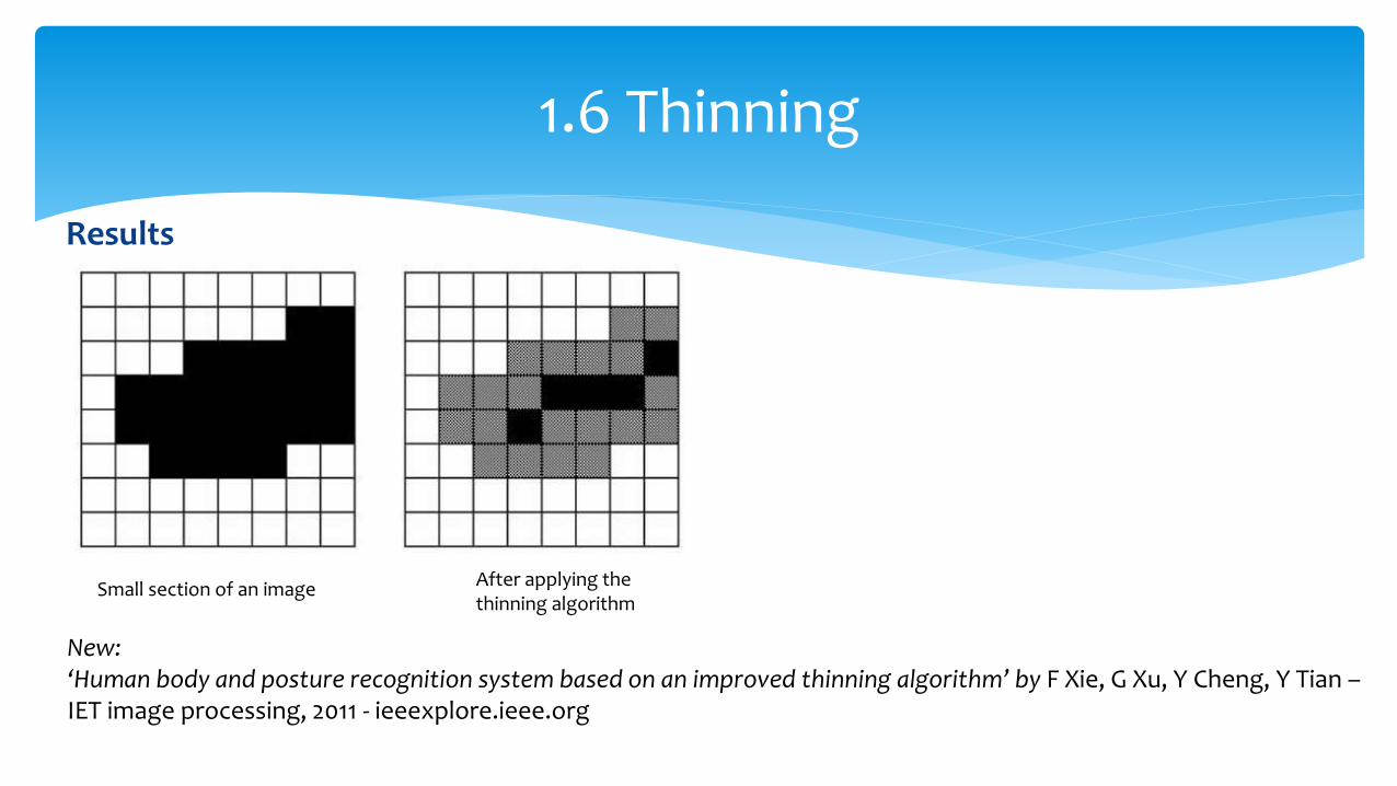
Results
1.6 Thinning
Small section of an image After applying the thinning algorithm
New: ‘Human body and posture recognition system based on an improved thinning algorithm’ by F Xie, G Xu, Y Cheng, Y Tian – IET image processing, 2011 - ieeexplore.ieee.org
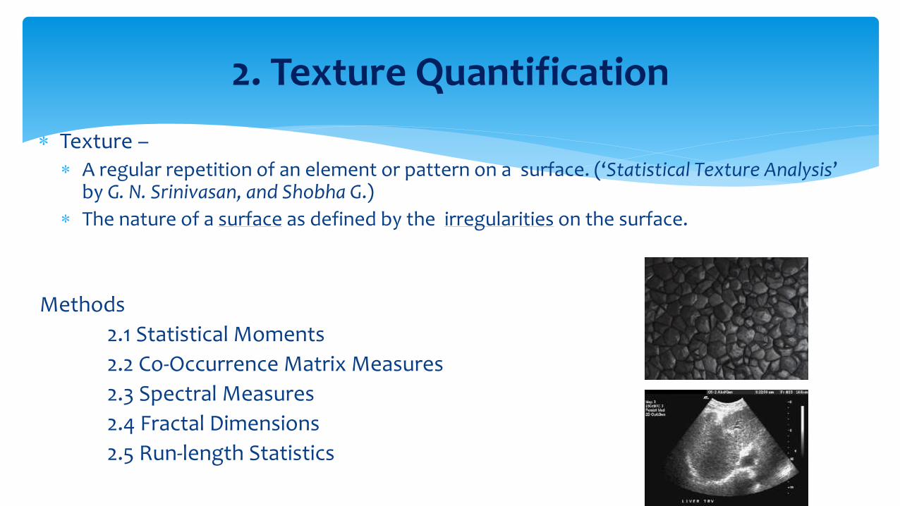
Texture – A regular repetition of an element or pattern on a surface. (‘Statistical Texture Analysis’
by G. N. Srinivasan, and Shobha G.)
The nature of a surface as defined by the irregularities on the surface.
Methods
2.1 Statistical Moments
2.2 Co-Occurrence Matrix Measures
2.3 Spectral Measures
2.4 Fractal Dimensions
2.5 Run-length Statistics
2. Texture Quantification
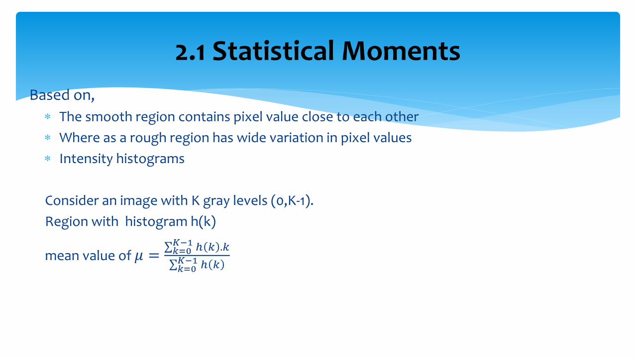
Based on,
The smooth region contains pixel value close to each other
Where as a rough region has wide variation in pixel values
Intensity histograms
Consider an image with K gray levels (0,K-1).
Region with histogram h(k)
mean value of 𝜇 = ℎ 𝑘 .𝑘𝐾−1𝑘=0
ℎ 𝑘𝐾−1𝑘=0
2.1 Statistical Moments
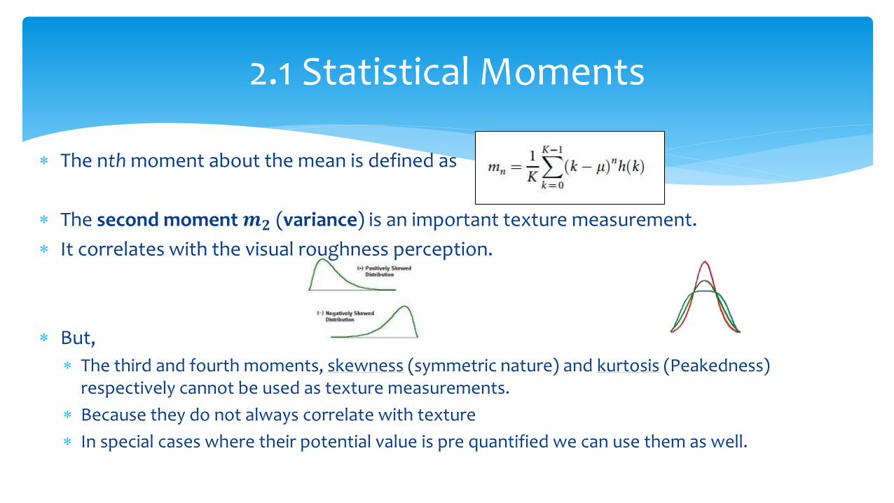
The nth moment about the mean is defined as
The second moment 𝒎𝟐 (variance) is an important texture measurement.
It correlates with the visual roughness perception.
But,
The third and fourth moments, skewness (symmetric nature) and kurtosis (Peakedness) respectively cannot be used as texture measurements.
Because they do not always correlate with texture
In special cases where their potential value is pre quantified we can use them as well.
2.1 Statistical Moments
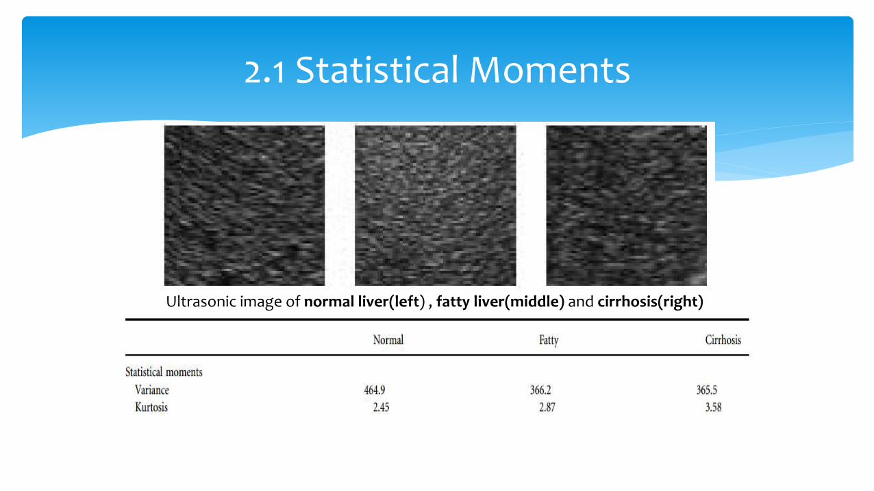
2.1 Statistical Moments
Ultrasonic image of normal liver(left) , fatty liver(middle) and cirrhosis(right)
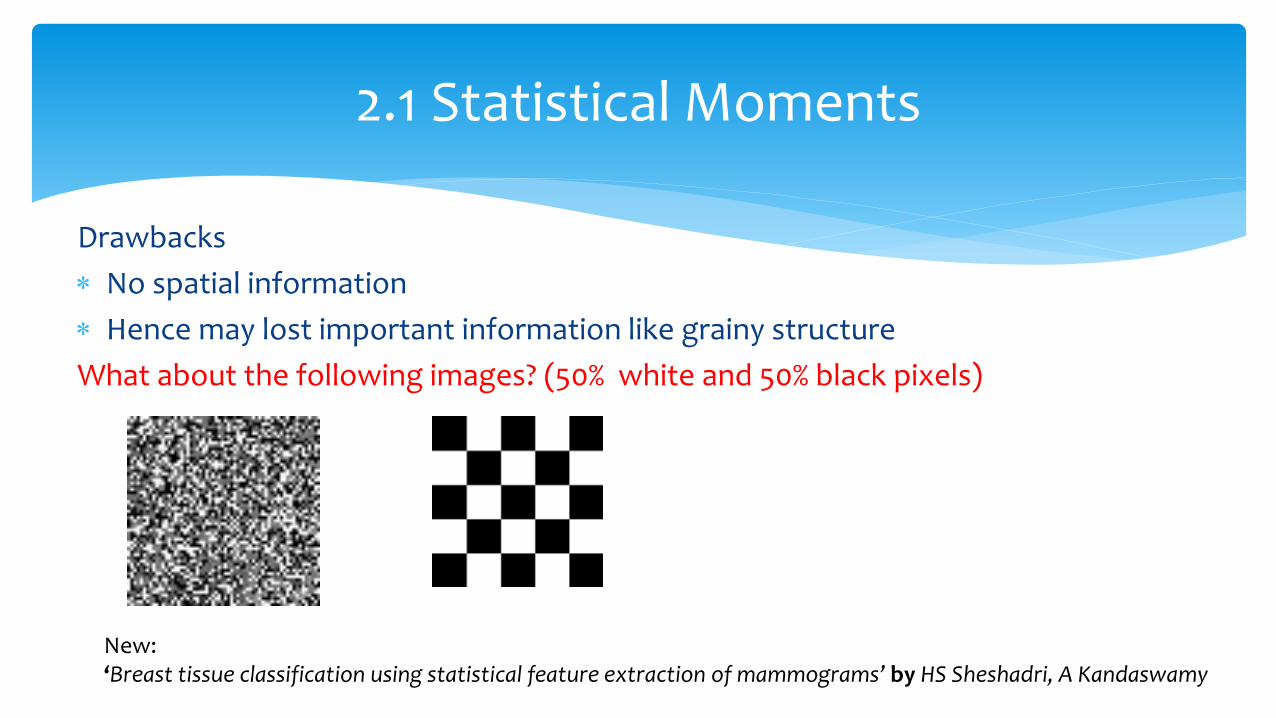
Drawbacks
No spatial information
Hence may lost important information like grainy structure
What about the following images? (50% white and 50% black pixels)
2.1 Statistical Moments
New: ‘Breast tissue classification using statistical feature extraction of mammograms’ by HS Sheshadri, A Kandaswamy
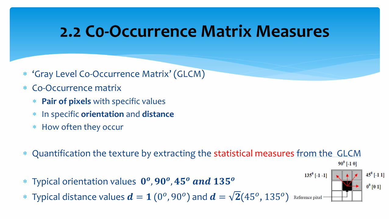
‘Gray Level Co-Occurrence Matrix’ (GLCM)
Co-Occurrence matrix
Pair of pixels with specific values
In specific orientation and distance
How often they occur
Quantification the texture by extracting the statistical measures from the GLCM
Typical orientation values 𝟎𝒐, 𝟗𝟎𝒐, 𝟒𝟓𝒐 𝒂𝒏𝒅 𝟏𝟑𝟓𝒐
Typical distance values 𝒅 = 𝟏 (0𝑜, 90𝑜) and 𝒅 = 𝟐(45𝑜, 135𝑜)
2.2 C0-Occurrence Matrix Measures
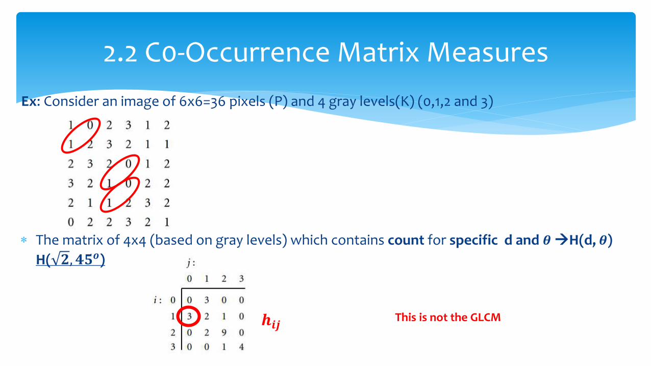
Ex: Consider an image of 6x6=36 pixels (P) and 4 gray levels(K) (0,1,2 and 3)
The matrix of 4x4 (based on gray levels) which contains count for specific d and 𝜽 H(d, 𝜽)
H( 𝟐, 𝟒𝟓𝒐)
2.2 C0-Occurrence Matrix Measures
This is not the GLCM 𝒉𝒊𝒋
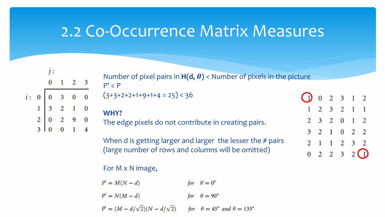
2.2 Co-Occurrence Matrix Measures
Number of pixel pairs in H(d, 𝜽) < Number of pixels in the picture P’ < P (3+3+2+2+1+9+1+4 = 25) < 36 WHY? The edge pixels do not contribute in creating pairs. When d is getting larger and larger the lesser the # pairs (large number of rows and columns will be omitted) For M x N image,
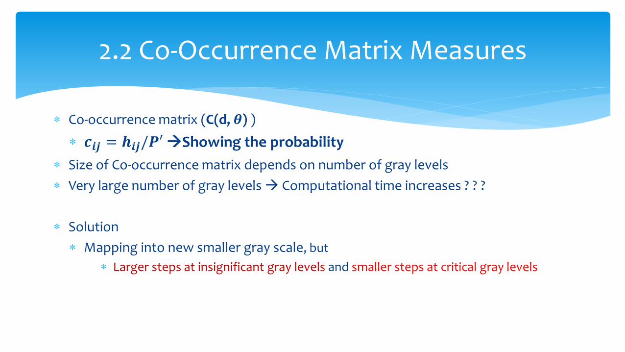
Co-occurrence matrix (C(d, 𝜽) )
𝒄𝒊𝒋 = 𝒉𝒊𝒋/𝑷′ Showing the probability
Size of Co-occurrence matrix depends on number of gray levels
Very large number of gray levels Computational time increases ? ? ?
Solution
Mapping into new smaller gray scale, but
Larger steps at insignificant gray levels and smaller steps at critical gray levels
2.2 Co-Occurrence Matrix Measures
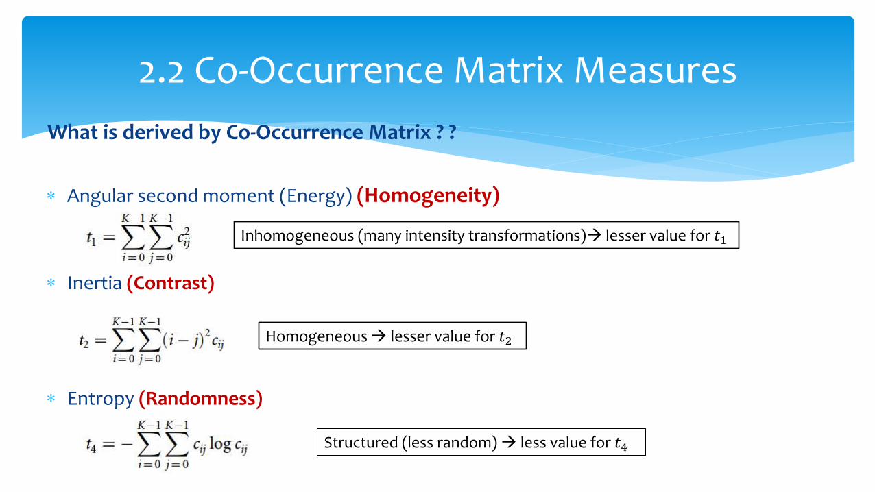
What is derived by Co-Occurrence Matrix ? ?
Angular second moment (Energy) (Homogeneity)
Inertia (Contrast)
Entropy (Randomness)
2.2 Co-Occurrence Matrix Measures
Inhomogeneous (many intensity transformations) lesser value for 𝑡1
Homogeneous lesser value for 𝑡2
Structured (less random) less value for 𝑡4
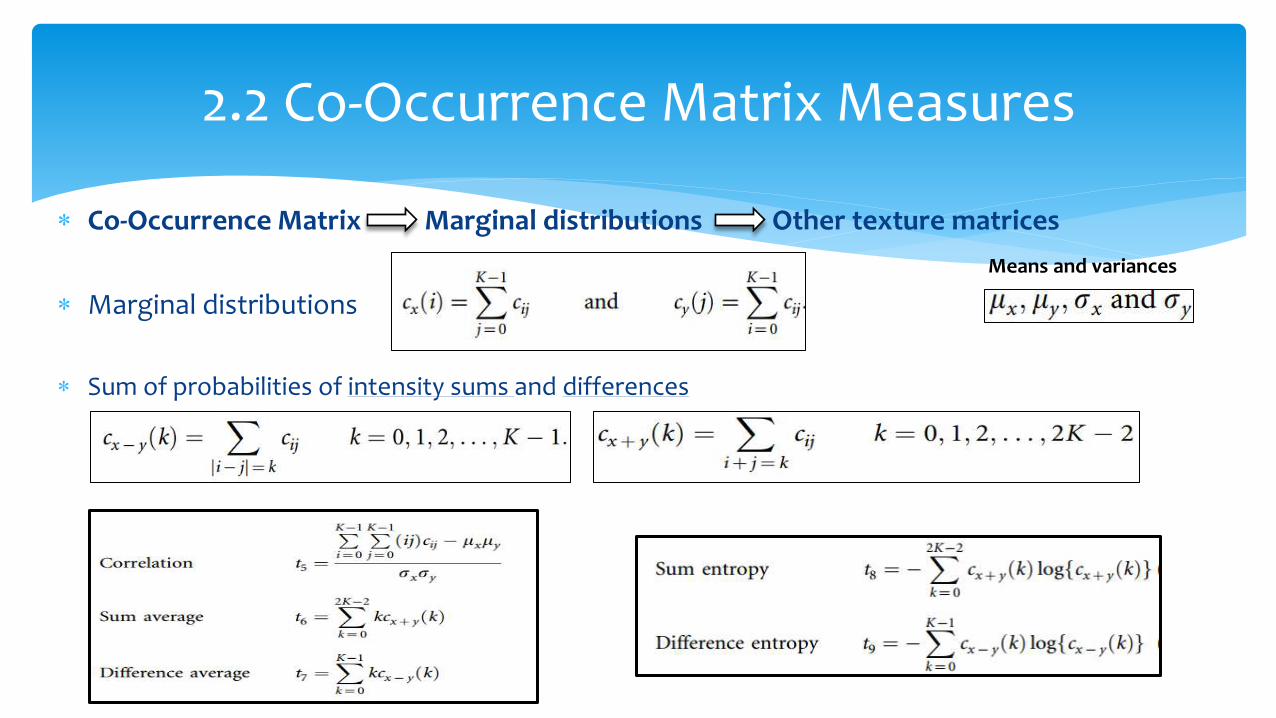
Co-Occurrence Matrix Marginal distributions Other texture matrices
Marginal distributions
Sum of probabilities of intensity sums and differences
2.2 Co-Occurrence Matrix Measures
Means and variances
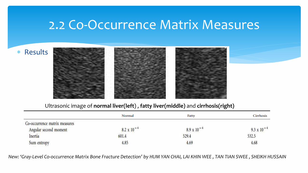
Results
2.2 Co-Occurrence Matrix Measures
Ultrasonic image of normal liver(left) , fatty liver(middle) and cirrhosis(right)
New: ‘Gray-Level Co-occurrence Matrix Bone Fracture Detection’ by HUM YAN CHAI, LAI KHIN WEE , TAN TIAN SWEE , SHEIKH HUSSAIN
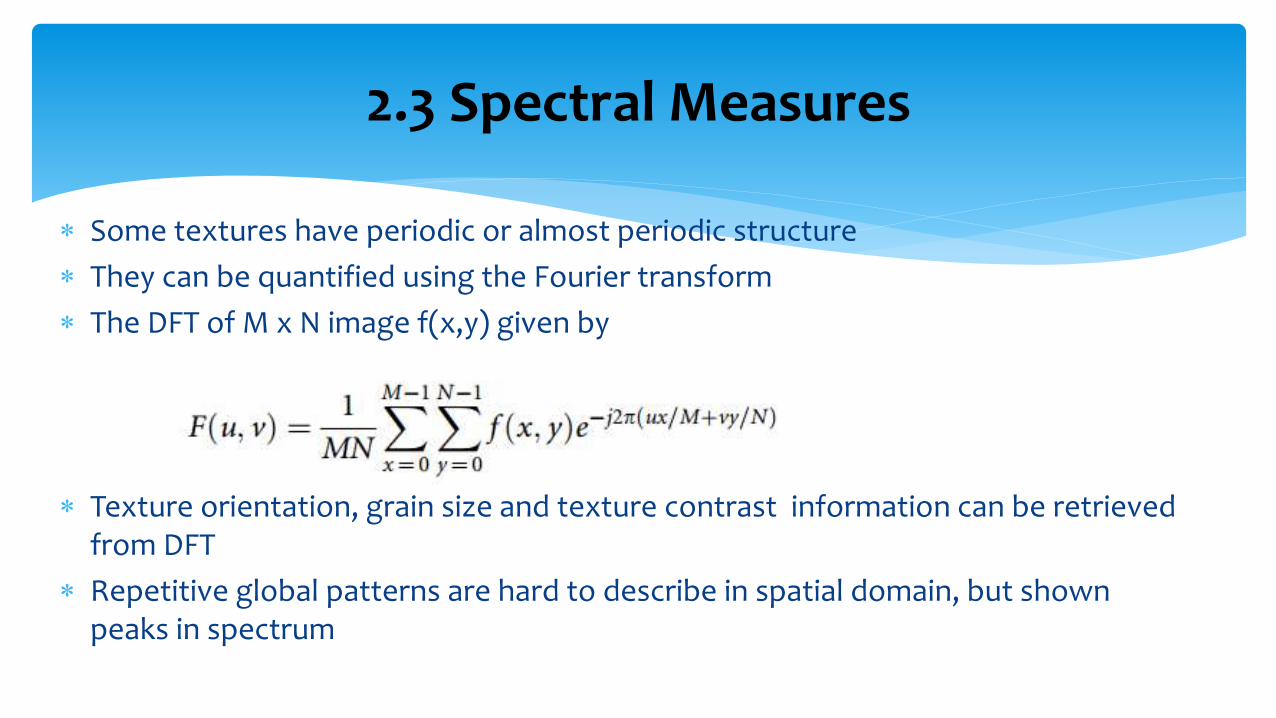
Some textures have periodic or almost periodic structure
They can be quantified using the Fourier transform
The DFT of M x N image f(x,y) given by
Texture orientation, grain size and texture contrast information can be retrieved from DFT
Repetitive global patterns are hard to describe in spatial domain, but shown peaks in spectrum
2.3 Spectral Measures
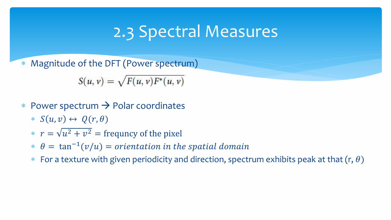
Magnitude of the DFT (Power spectrum)
Power spectrum Polar coordinates
𝑆 𝑢, 𝑣 ↔ 𝑄(𝑟, 𝜃)
𝑟 = 𝑢2 + 𝑣2 = frequncy of the pixel
𝜃 = tan−1(𝑣/𝑢) = 𝑜𝑟𝑖𝑒𝑛𝑡𝑎𝑡𝑖𝑜𝑛 𝑖𝑛 𝑡ℎ𝑒 𝑠𝑝𝑎𝑡𝑖𝑎𝑙 𝑑𝑜𝑚𝑎𝑖𝑛
For a texture with given periodicity and direction, spectrum exhibits peak at that (r, 𝜃)
2.3 Spectral Measures
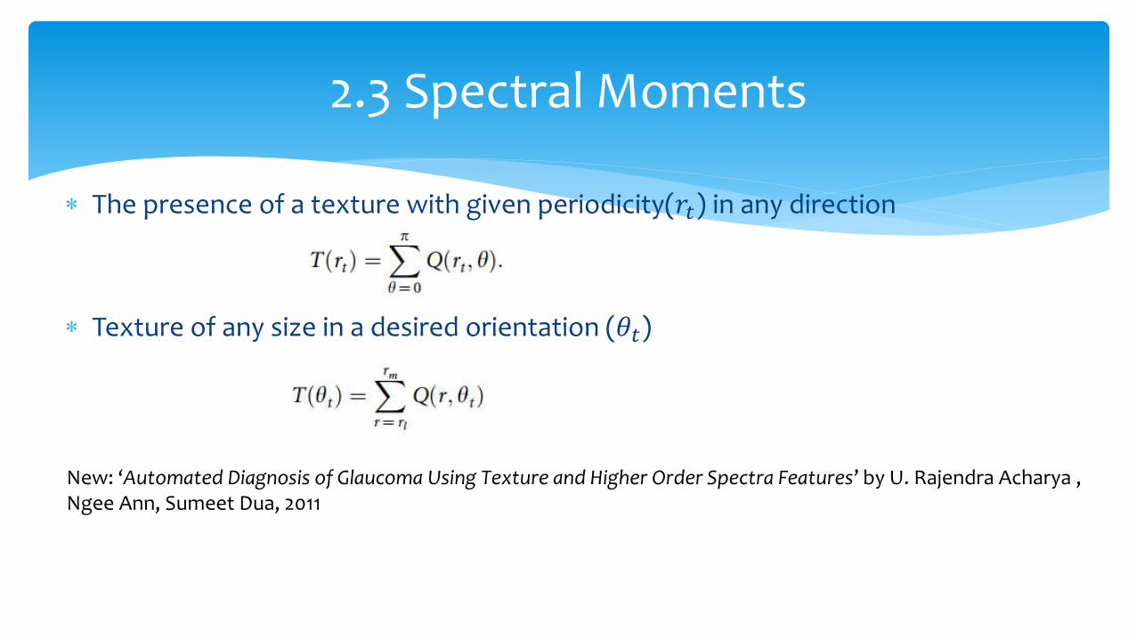
The presence of a texture with given periodicity(𝑟𝑡) in any direction
Texture of any size in a desired orientation (𝜃𝑡)
New: ‘Automated Diagnosis of Glaucoma Using Texture and Higher Order Spectra Features’ by U. Rajendra Acharya , Ngee Ann, Sumeet Dua, 2011
2.3 Spectral Moments
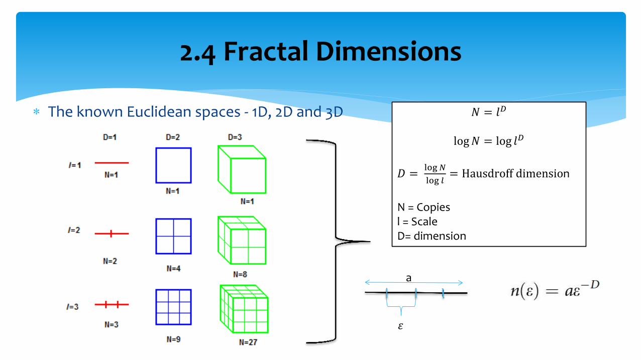
The known Euclidean spaces - 1D, 2D and 3D
2.4 Fractal Dimensions
𝑁 = 𝑙𝐷
log𝑁 = log 𝑙𝐷
𝐷 = log 𝑁
log 𝑙= Hausdroff dimension
N = Copies l = Scale D= dimension
a
𝜀
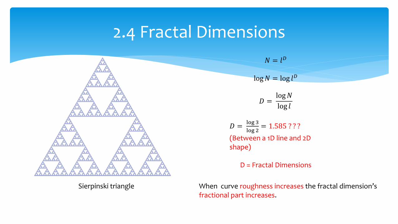
2.4 Fractal Dimensions
Sierpinski triangle
𝑁 = 𝑙𝐷
log𝑁 = log 𝑙𝐷
𝐷 = log𝑁
log 𝑙
𝐷 = log 3
log 2= 1.585 ? ? ?
(Between a 1D line and 2D shape)
D = Fractal Dimensions
When curve roughness increases the fractal dimension’s fractional part increases.
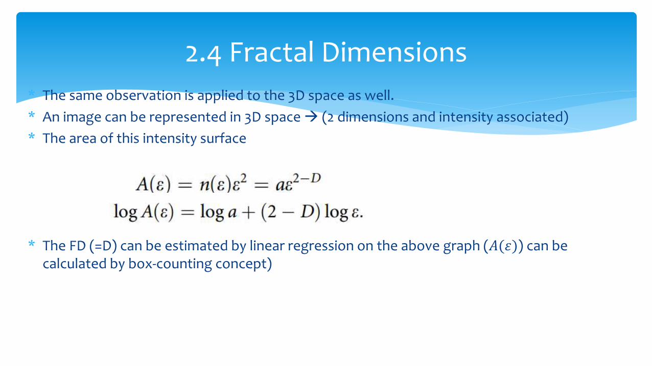
* The same observation is applied to the 3D space as well.
* An image can be represented in 3D space (2 dimensions and intensity associated)
* The area of this intensity surface
* The FD (=D) can be estimated by linear regression on the above graph (𝐴(𝜀)) can be calculated by box-counting concept)
2.4 Fractal Dimensions
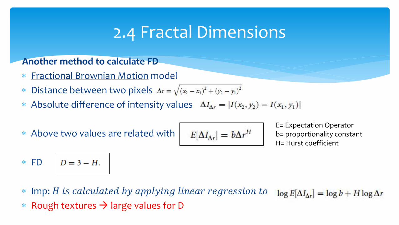
Another method to calculate FD
Fractional Brownian Motion model
Distance between two pixels
Absolute difference of intensity values
Above two values are related with
FD
Imp: 𝐻 𝑖𝑠 𝑐𝑎𝑙𝑐𝑢𝑙𝑎𝑡𝑒𝑑 𝑏𝑦 𝑎𝑝𝑝𝑙𝑦𝑖𝑛𝑔 𝑙𝑖𝑛𝑒𝑎𝑟 𝑟𝑒𝑔𝑟𝑒𝑠𝑠𝑖𝑜𝑛 𝑡𝑜
Rough textures large values for D
2.4 Fractal Dimensions
E= Expectation Operator b= proportionality constant H= Hurst coefficient
2.4 Fractal Dimensions
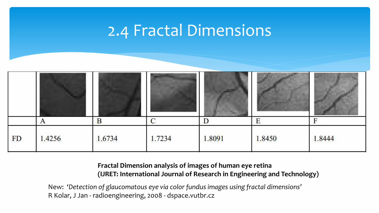
Fractal Dimension analysis of images of human eye retina (IJRET: International Journal of Research in Engineering and Technology)
New: ‘Detection of glaucomatous eye via color fundus images using fractal dimensions’ R Kolar, J Jan - radioengineering, 2008 - dspace.vutbr.cz
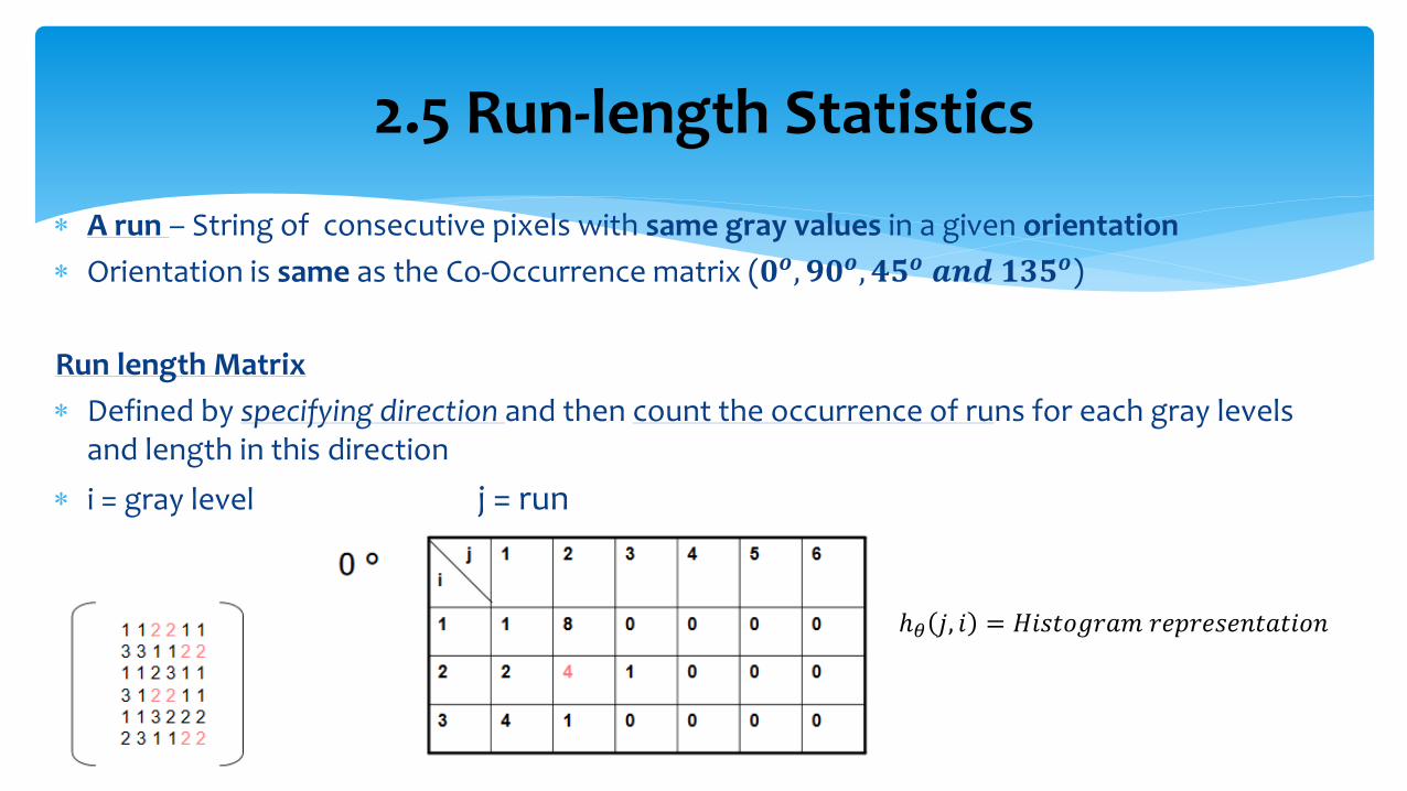
A run – String of consecutive pixels with same gray values in a given orientation
Orientation is same as the Co-Occurrence matrix (𝟎𝒐, 𝟗𝟎𝒐, 𝟒𝟓𝒐 𝒂𝒏𝒅 𝟏𝟑𝟓𝒐)
Run length Matrix
Defined by specifying direction and then count the occurrence of runs for each gray levels and length in this direction
i = gray level j = run
2.5 Run-length Statistics
ℎ𝜃 𝑗, 𝑖 = 𝐻𝑖𝑠𝑡𝑜𝑔𝑟𝑎𝑚 𝑟𝑒𝑝𝑟𝑒𝑠𝑒𝑛𝑡𝑎𝑡𝑖𝑜𝑛
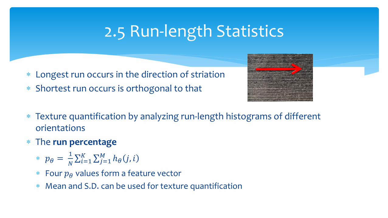
Longest run occurs in the direction of striation
Shortest run occurs is orthogonal to that
Texture quantification by analyzing run-length histograms of different orientations
The run percentage
𝑝𝜃 = 1
𝑁 ℎ𝜃 𝑗, 𝑖
𝑀𝑗=1
𝐾𝑖=1
Four 𝑝𝜃 values form a feature vector
Mean and S.D. can be used for texture quantification
2.5 Run-length Statistics

Thank you!


