
Multi-Factor Experiments
Twoway anova
Interactions
More than two factors
ETH – p. 1/31

Hypertension: Effect of biofeedback
Biofeedback Biofeedback Medication Control
+ Medication
158 188 186 185
163 183 191 190
173 198 196 195
178 178 181 200
168 193 176 180
ETH – p. 2/31
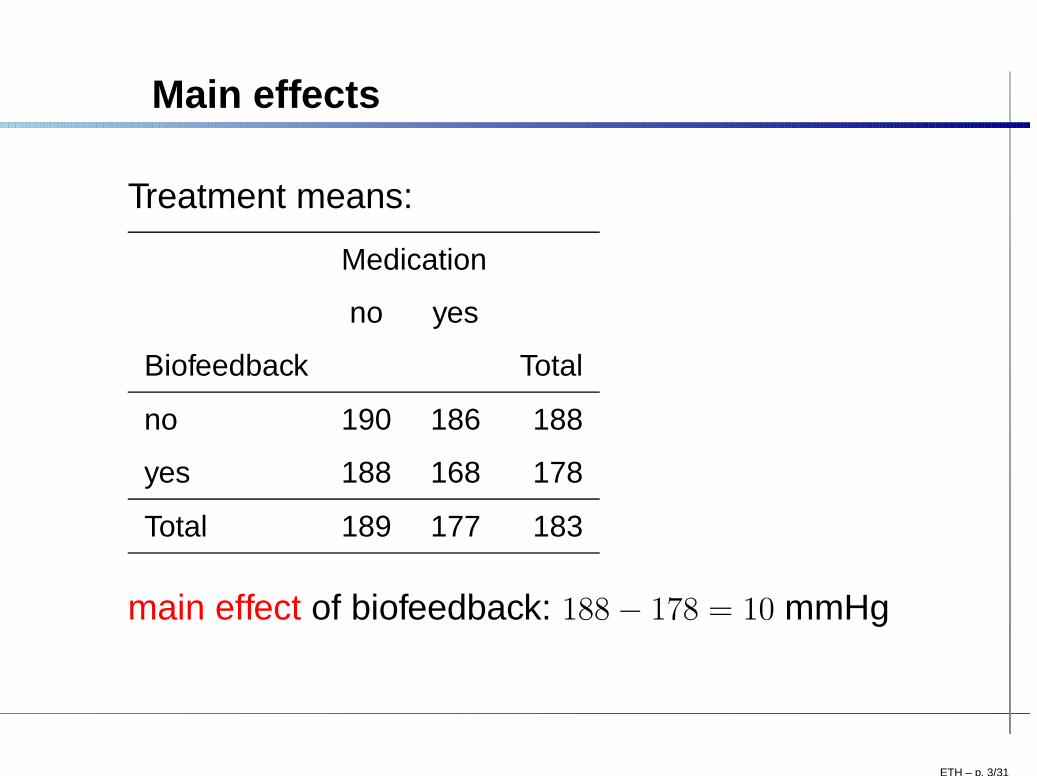
Main effects
Treatment means:
Medication
no yes
Biofeedback Total
no 190 186 188
yes 188 168 178
Total 189 177 183
main effect of biofeedback: 188 − 178 = 10 mmHg
ETH – p. 3/31
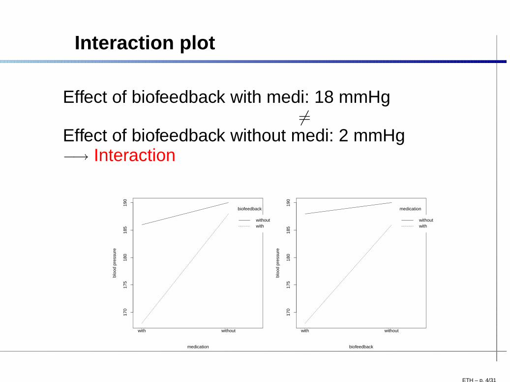
Interaction plot
Effect of biofeedback with medi: 18 mmHg6=
Effect of biofeedback without medi: 2 mmHg−→ Interaction
medication
bloo
d pr
essu
re
170
175
180
185
190
with without
biofeedback
withoutwith
biofeedback
bloo
d pr
essu
re
170
175
180
185
190
with without
medication
withoutwith
ETH – p. 4/31
Model for two factors
Yijk = µ + Ai + Bj + (AB)ij + ǫijk
i = 1, . . . , I; j = 1, . . . , J ; k = 1, . . . , n.∑
Ai = 0,∑
Bj = 0,∑
i(AB)ij =∑
j(AB)ij = 0.
Ai : ith effect of factor A
Bj : jth effect of factor B
µ + Ai + Bj : overall mean + effect of factor A on level i+ effect of factor B on level j
(AB)ij : deviation from additive model
ETH – p. 5/31
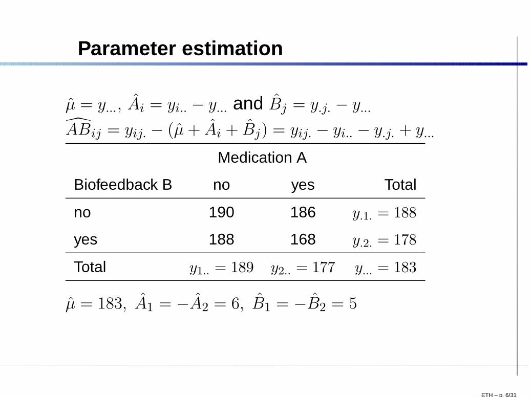
Parameter estimation
µ = y..., Ai = yi.. − y... and Bj = y.j. − y...
ABij = yij. − (µ + Ai + Bj) = yij. − yi.. − y.j. + y...
Medication A
Biofeedback B no yes Total
no 190 186 y.1. = 188
yes 188 168 y.2. = 178
Total y1.. = 189 y2.. = 177 y... = 183
µ = 183, A1 = −A2 = 6, B1 = −B2 = 5
ETH – p. 6/31
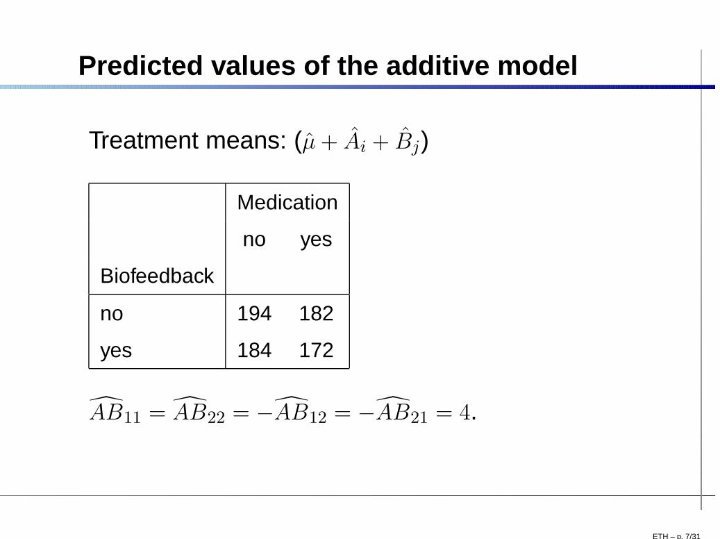
Predicted values of the additive model
Treatment means: (µ + Ai + Bj)
Medication
no yes
Biofeedback
no 194 182
yes 184 172
AB11 = AB22 = −AB12 = −AB21 = 4.
ETH – p. 7/31
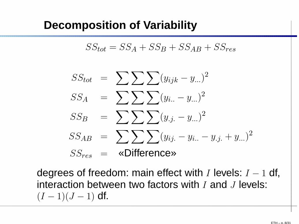
Decomposition of Variability
SStot = SSA + SSB + SSAB + SSres
SStot =∑ ∑ ∑
(yijk − y...)2
SSA =∑ ∑ ∑
(yi.. − y...)2
SSB =∑ ∑ ∑
(y.j. − y...)2
SSAB =∑ ∑ ∑
(yij. − yi.. − y.j. + y...)2
SSres = «Difference»
degrees of freedom: main effect with I levels: I − 1 df,interaction between two factors with I and J levels:(I − 1)(J − 1) df.
ETH – p. 8/31
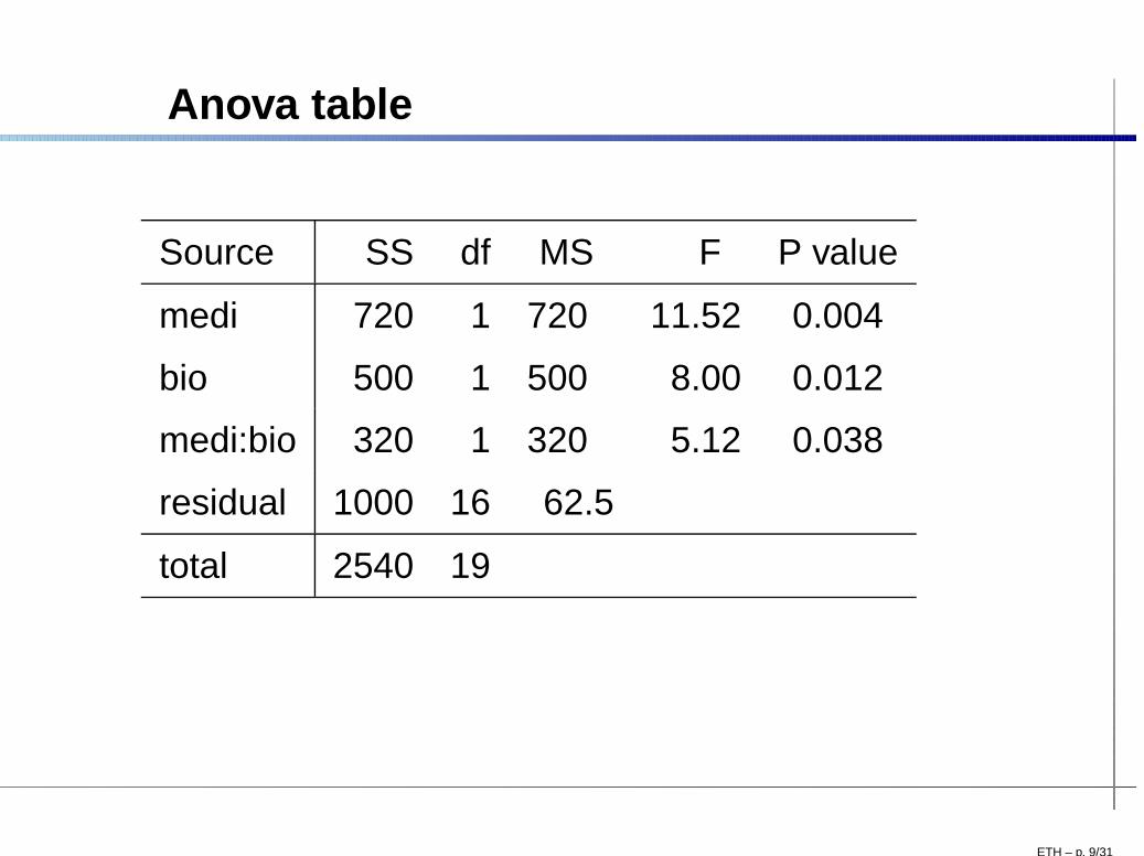
Anova table
Source SS df MS F P value
medi 720 1 720 11.52 0.004
bio 500 1 500 8.00 0.012
medi:bio 320 1 320 5.12 0.038
residual 1000 16 62.5
total 2540 19
ETH – p. 9/31

Treatment effects
effect size C.I.
medi without bio: y21. − y11. = 186 − 190 = −4 (−18, 10)
medi with bio: y22. − y12. = 168 − 188 = −20 (−34,−6)
bio without medi: y12. − y11. = 188 − 190 = −2 (−16, 12)
bio with medi: y22. − y21. = 168 − 186 = −18 (−32,−4)
(standard error:√
2·MSres/5 = 5)
ETH – p. 10/31

Efficiency of factorials
factorial
medication
biofeedback no yes
no 6 6
yes 6 6
Two separate studies
medication biofeedback
no yes and no yes
6 6 6 6
or:
control medi bio
8 8 8
ETH – p. 11/31
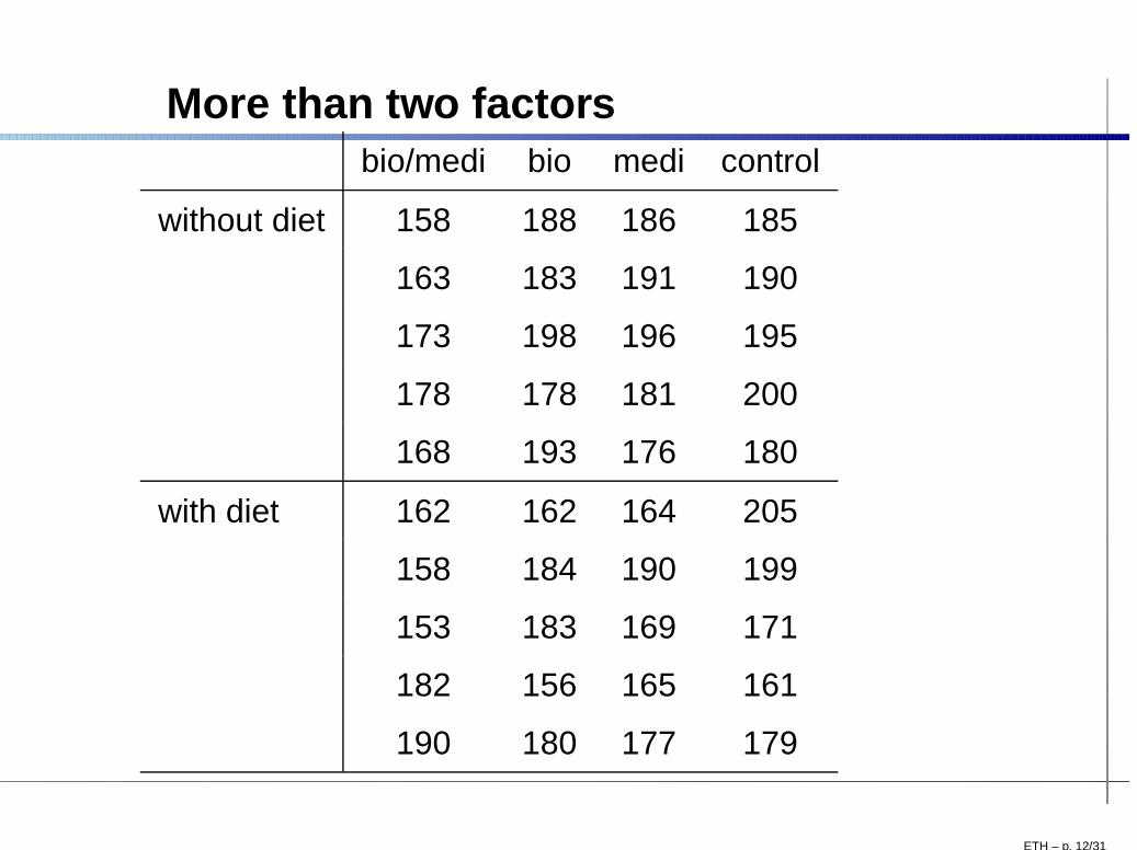
More than two factorsbio/medi bio medi control
without diet 158 188 186 185
163 183 191 190
173 198 196 195
178 178 181 200
168 193 176 180
with diet 162 162 164 205
158 184 190 199
153 183 169 171
182 156 165 161
190 180 177 179
ETH – p. 12/31

Treatment means
without diet(C)
medication (A)
bio (B) no yes total
no 190 186 188
yes 188 168 178
total 189 177 183
with diet (C)
medication (A)
bio (B) no yes total
no 183 173 178
yes 173 169 171
total 178 171 174.5
ETH – p. 13/31
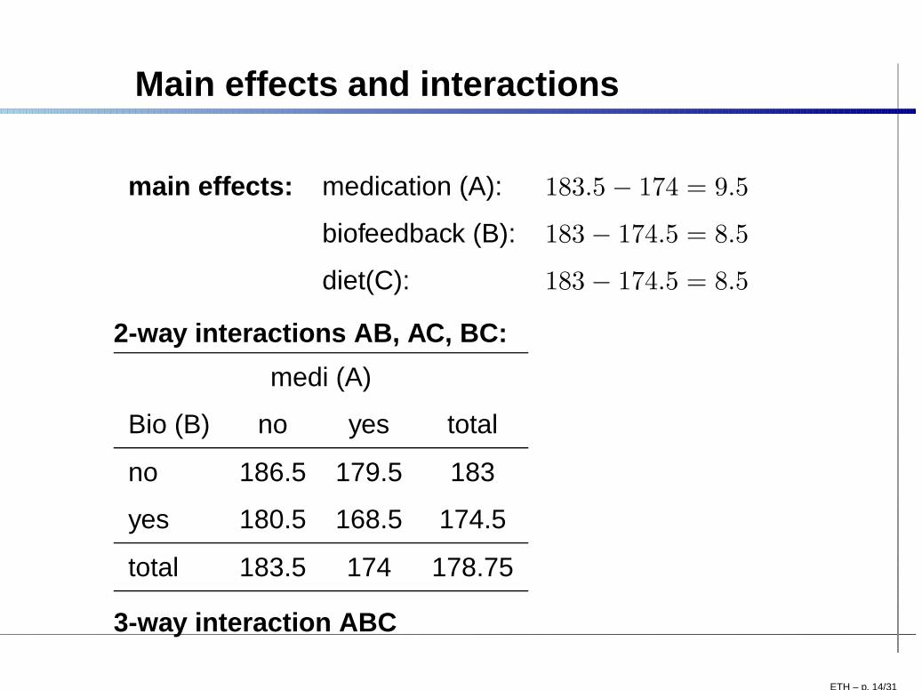
Main effects and interactions
main effects: medication (A): 183.5 − 174 = 9.5
biofeedback (B): 183 − 174.5 = 8.5
diet(C): 183 − 174.5 = 8.5
2-way interactions AB, AC, BC:
medi (A)
Bio (B) no yes total
no 186.5 179.5 183
yes 180.5 168.5 174.5
total 183.5 174 178.75
3-way interaction ABC
ETH – p. 14/31

Model and Anova table
Yijkl = µ+Ai+Bj+Ck+(AB)ij+(AC)ik+(BC)jk+(ABC)ijk+ǫijkl
∑Ai = 0, . . . ,
∑k(ABC)ijk = 0
Source df MS=SS/df F
A I − 1 MSA/MSres
B J − 1 MSB/MSres
C K − 1 MSC/MSres
AB (I − 1)(J − 1) MSAB/MSres
AC (I − 1)(K − 1) MSAC/MSres
BC (J − 1)(K − 1) MSBC/MSres
ABC (I − 1)(J − 1)(K − 1) MSABC/MSres
Residual «Difference» MSres = σ2
Total IJKn − 1ETH – p. 15/31

Anova table
Source SS df MS F P value
medi 902.5 1 902.5 6.33 0.017
bio 722.5 1 722.5 5.06 0.031
diet 722.5 1 722.5 5.06 0.031
medi:bio 62.5 1 62.5 0.44 0.51
medi:diet 62.5 1 62.5 0.44 0.51
bio:diet 22.5 1 22.5 0.16 0.69
medi:bio:diet 302.5 1 302.5 2.12 0.15
Residual 4566.0 32 142.7
Total 7363.5 39
ETH – p. 16/31
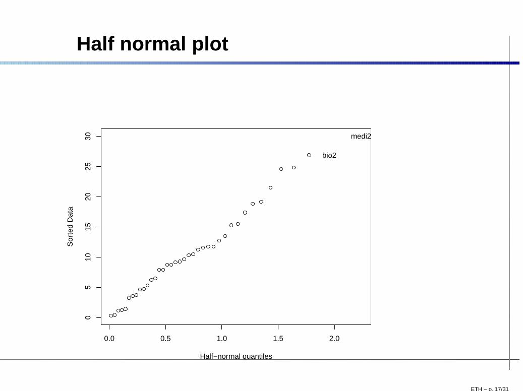
Half normal plot
0.0 0.5 1.0 1.5 2.0
05
1015
2025
30
Half−normal quantiles
Sor
ted
Dat
a
bio2
medi2
ETH – p. 17/31

Unbalanced Factorials
uncorrelated estimators:
SStot = SSA + SSB + SSAB + SSres︸ ︷︷ ︸SSC+...+SSres′
correlated estimators:
SStot = SS′
A + SS′
B + SS′
AB + SSC + . . . + SSres′
SS Typ I: SSA ignores all other SS
SS Typ II: SSA takes into account all other main effects,ignores all interactions
SS Typ III: SSA takes into account all other effects
ETH – p. 18/31
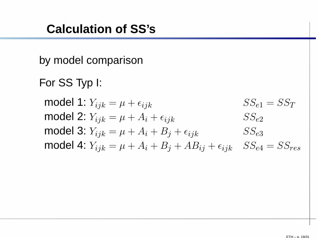
Calculation of SS’s
by model comparison
For SS Typ I:
model 1: Yijk = µ + ǫijk SSe1 = SST
model 2: Yijk = µ + Ai + ǫijk SSe2
model 3: Yijk = µ + Ai + Bj + ǫijk SSe3
model 4: Yijk = µ + Ai + Bj + ABij + ǫijk SSe4 = SSres
ETH – p. 19/31
Rat genotype
Litters of rats are separated from their naturalmother and given to another female to raise.
2 factors: mother’s genotype (A, B, I, J) and litter’sgenotype (A, B, I, J)
response: average weight gain of the litter.
ETH – p. 20/31
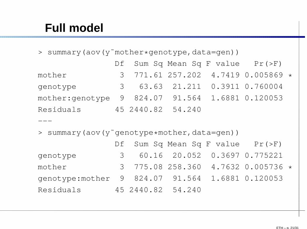
Full model
> summary(aov(y˜mother * genotype,data=gen))
Df Sum Sq Mean Sq F value Pr(>F)
mother 3 771.61 257.202 4.7419 0.005869 *genotype 3 63.63 21.211 0.3911 0.760004
mother:genotype 9 824.07 91.564 1.6881 0.120053
Residuals 45 2440.82 54.240
---
> summary(aov(y˜genotype * mother,data=gen))
Df Sum Sq Mean Sq F value Pr(>F)
genotype 3 60.16 20.052 0.3697 0.775221
mother 3 775.08 258.360 4.7632 0.005736 *genotype:mother 9 824.07 91.564 1.6881 0.120053
Residuals 45 2440.82 54.240
ETH – p. 21/31
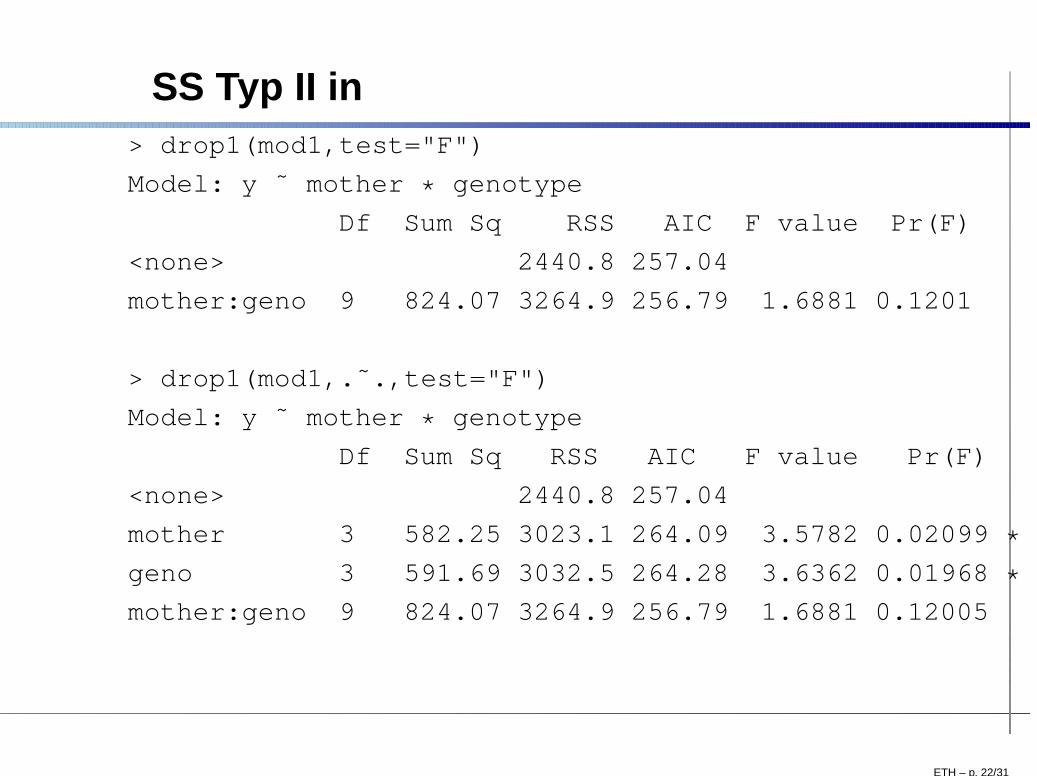
SS Typ II in> drop1(mod1,test="F")
Model: y ˜ mother * genotype
Df Sum Sq RSS AIC F value Pr(F)
<none> 2440.8 257.04
mother:geno 9 824.07 3264.9 256.79 1.6881 0.1201
> drop1(mod1,.˜.,test="F")
Model: y ˜ mother * genotype
Df Sum Sq RSS AIC F value Pr(F)
<none> 2440.8 257.04
mother 3 582.25 3023.1 264.09 3.5782 0.02099 *geno 3 591.69 3032.5 264.28 3.6362 0.01968 *mother:geno 9 824.07 3264.9 256.79 1.6881 0.12005
ETH – p. 22/31
Offer for a 6-year old car
Planned experiment to see whether the offeredcash for the same medium-priced car depends ongender or age (young, middle, elderly) of the seller.
6 factor combinations with 6 replications each.
Response variable y is offer made by a car dealer(in $ 100)
Covariable: overall sales volume of the dealer
ETH – p. 23/31

Analysis of Covariance
Covariates can reduce MSres, thereby increasingpower for testing.
Baseline or pretest values are often used ascovariates. A covariate can adjust for differences incharacteristics of subjects in the treatment groups.
It should be related only to the response variableand not to the treatment variables (factors).
We assume that the covariate will be linearlyrelated to the response and that the relationshipwill be the same for all levels of the factor (nointeraction between covariate and factors).
ETH – p. 24/31
Model for two-way ANCOVA
Yijk = µ + θxijk + Ai + Bj + (AB)ij + ǫijk
∑Ai =
∑Bj =
∑(AB)ij = 0, ǫijk ∼ N (0, σ2)
ETH – p. 25/31

Effect of Age and Gender
young middle elderly
20
22
24
26
28
30
y
male female
20
22
24
26
28
30
y
ETH – p. 26/31

Interaction effect of Age and Gender
2224
2628
cash$age
mea
n of
cas
h$y
young middle elderly
cash$gender
malefemale
2224
2628
cash$gender
mea
n of
cas
h$y
male female
cash$age
middleyoungelderly
ETH – p. 27/31
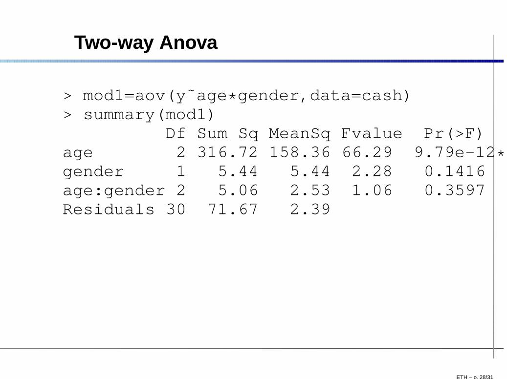
Two-way Anova
> mod1=aov(y˜age * gender,data=cash)> summary(mod1)
Df Sum Sq MeanSq Fvalue Pr(>F)age 2 316.72 158.36 66.29 9.79e-12 ***gender 1 5.44 5.44 2.28 0.1416age:gender 2 5.06 2.53 1.06 0.3597Residuals 30 71.67 2.39
ETH – p. 28/31

Sales and Cash Offer
1 2 3 4 5 6
2022
2426
2830
cash$sales
cash
$y
ETH – p. 29/31

Sales and Cash Offer by Group
sales
y
20
22
24
26
28
30
1 2 3 4 5 6
youngmale
middlemale
1 2 3 4 5 6
elderlymale
youngfemale
1 2 3 4 5 6
middlefemale
20
22
24
26
28
30
elderlyfemale
ETH – p. 30/31
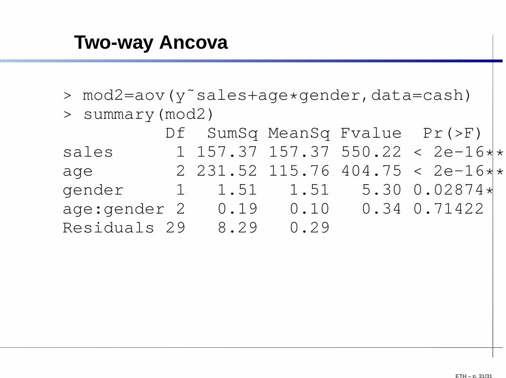
Two-way Ancova
> mod2=aov(y˜sales+age * gender,data=cash)> summary(mod2)
Df SumSq MeanSq Fvalue Pr(>F)sales 1 157.37 157.37 550.22 < 2e-16 ***age 2 231.52 115.76 404.75 < 2e-16 ***gender 1 1.51 1.51 5.30 0.02874 *age:gender 2 0.19 0.10 0.34 0.71422Residuals 29 8.29 0.29
ETH – p. 31/31


