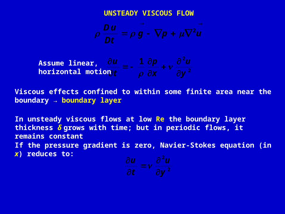
UNSTEADY VISCOUS FLOW
upgDt
uD
2
2
21
y
u
x
p
t
u
Viscous effects confined to within some finite area near the boundary → boundary layer
In unsteady viscous flows at low Re the boundary layer thickness δ grows with time; but in periodic flows, it remains constant
If the pressure gradient is zero, Navier-Stokes equation (in x) reduces to:
2
2
y
u
t
u
Assume linear, horizontal motion
2
2
y
u
t
u
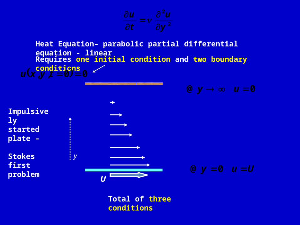
Heat Equation– parabolic partial differential equation - linear
Requires one initial condition and two boundary conditions
U
y
Uuy 0@
0@ uy
00,, tyxu
Total of three conditions
Impulsively started plate –
Stokes first problem
2
2
y
u
t
u
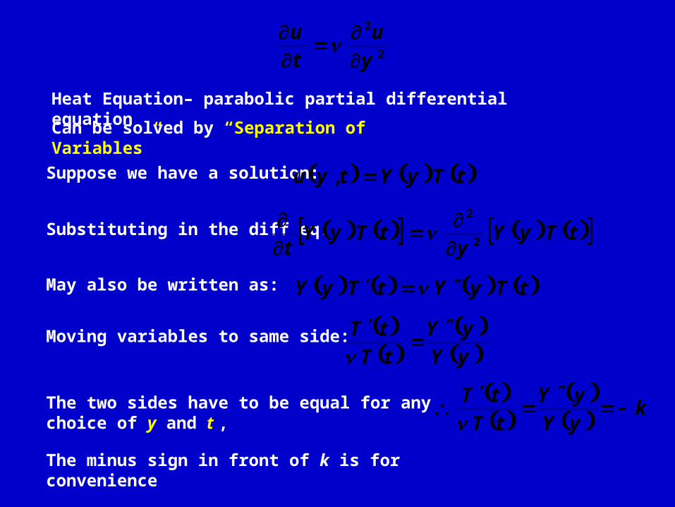
Heat Equation– parabolic partial differential equation
Can be solved by “Separation of Variables”
Suppose we have a solution: tTyYtyu ,
Substituting in the diff eq: tTyYy
tTyYt 2
2
May also be written as: tTyYtTyY
Moving variables to same side:
yY
yY
tT
tT
The two sides have to be equal for any choice of y and t ,
kyY
yY
tT
tT
The minus sign in front of k is for convenience
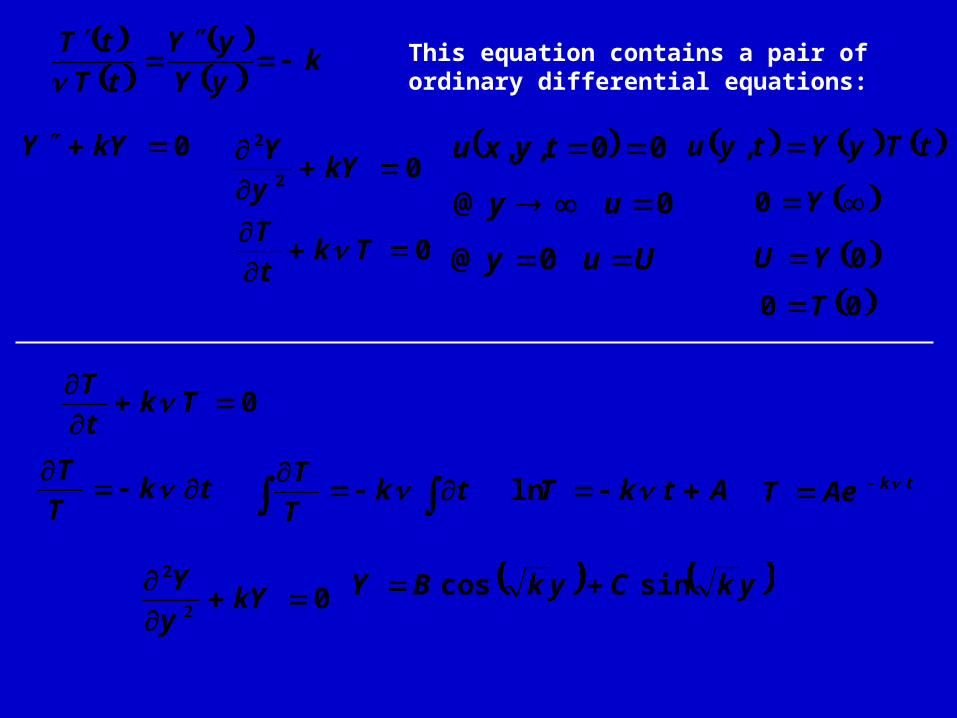
This equation contains a pair of ordinary differential equations:
kyY
yY
tT
tT
0
0
TkT
kYY
0
02
2
Tkt
T
kYy
Y
Uuy 0@
0@ uy
00,, tyxu tTyYtyu ,
0YU
Y0
00 T
0
Tkt
T
tkT
T
tkT
T AtkT ln tkAeT
02
2
kYy
Y ykCykBY sincos

t
y
Ueu 4
2
ykCykBY sincos tTyYtyu ,
increasing time
2
L
nkn
Applying B.C.,B = 0; C =1;
L
yneAu
tL
n
n
sin
2

2
2
y
u
t
u
Uuy 0@
0@ uy
00,, tyxu
New independent variable:t
y
2
η is used to transform heat equation:
d
d
td
d
tt 2
d
d
td
d
yy 2
1
2
2
2
2
4
1
d
d
ty
Substituting into heat equation:
2
2
42
d
ud
td
du
t
Alternative solution to“Separation of Variables” – “Similarity Solution”
from:2y
u
t
u
022
2
d
du
d
ud

022
2
d
du
d
ud
Uu 0@
0@ u
asu 0
To transform second order into first order: d
duf
2 BC turn into 1
02 fd
df
With solution:2Aef
Integrating to obtain u:
BdeAu
0
2
Or in terms of the error function:
deerf0
22 erfUu 1
df
df2
erf
2e
For η > 2 the error function is nearly 1, so that u → 0
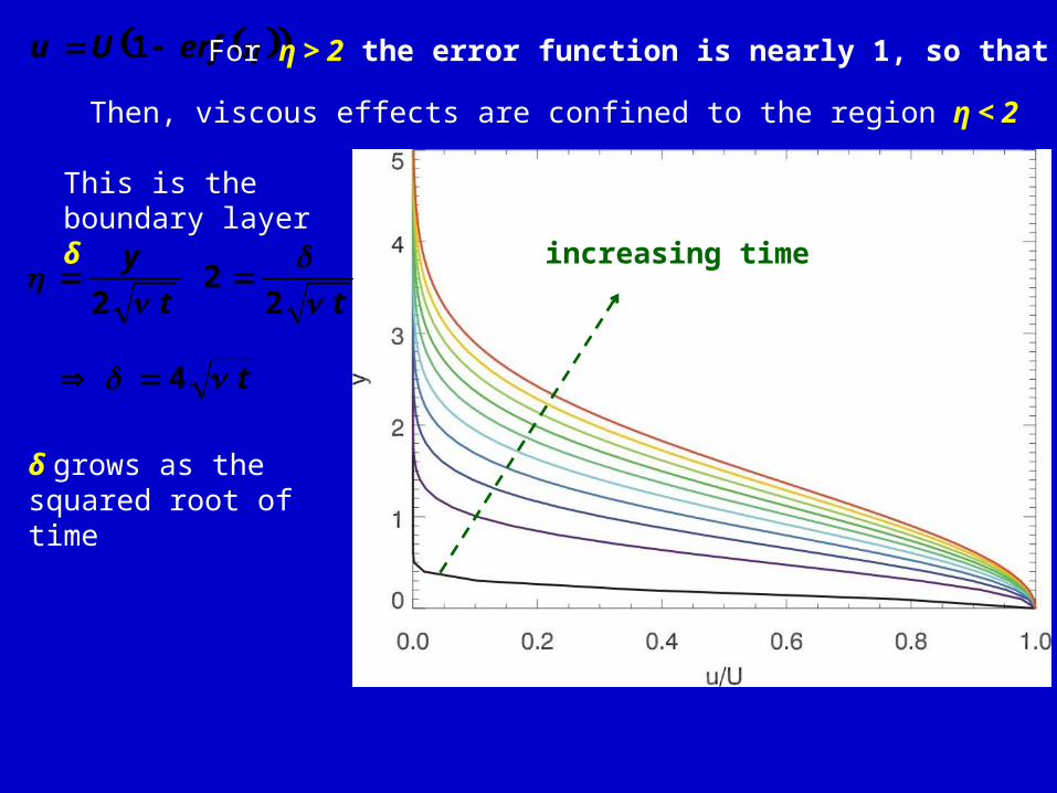
erfUu 1 For η > 2 the error function is nearly 1, so that u → 0
Then, viscous effects are confined to the region η < 2
This is the boundary layer δ
t
y
2
t
22
t 4
δ grows as the squared root of time
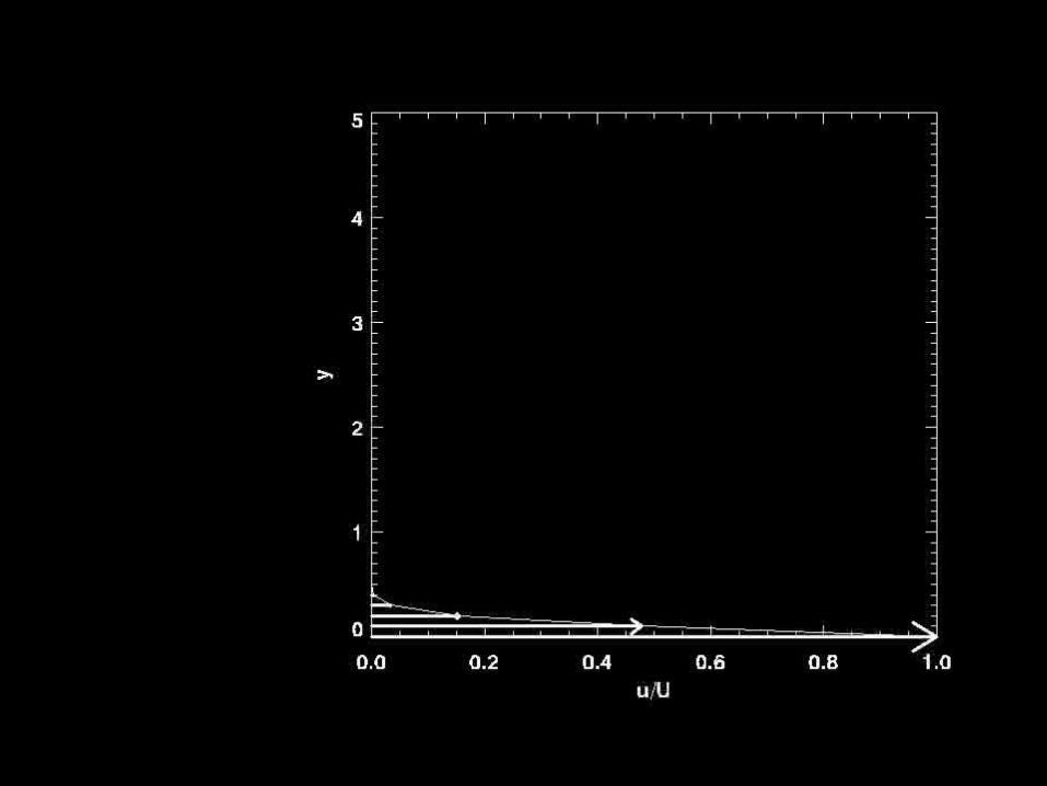
increasing time
erfUu 1
t
y
2
2
2
y
u
t
u
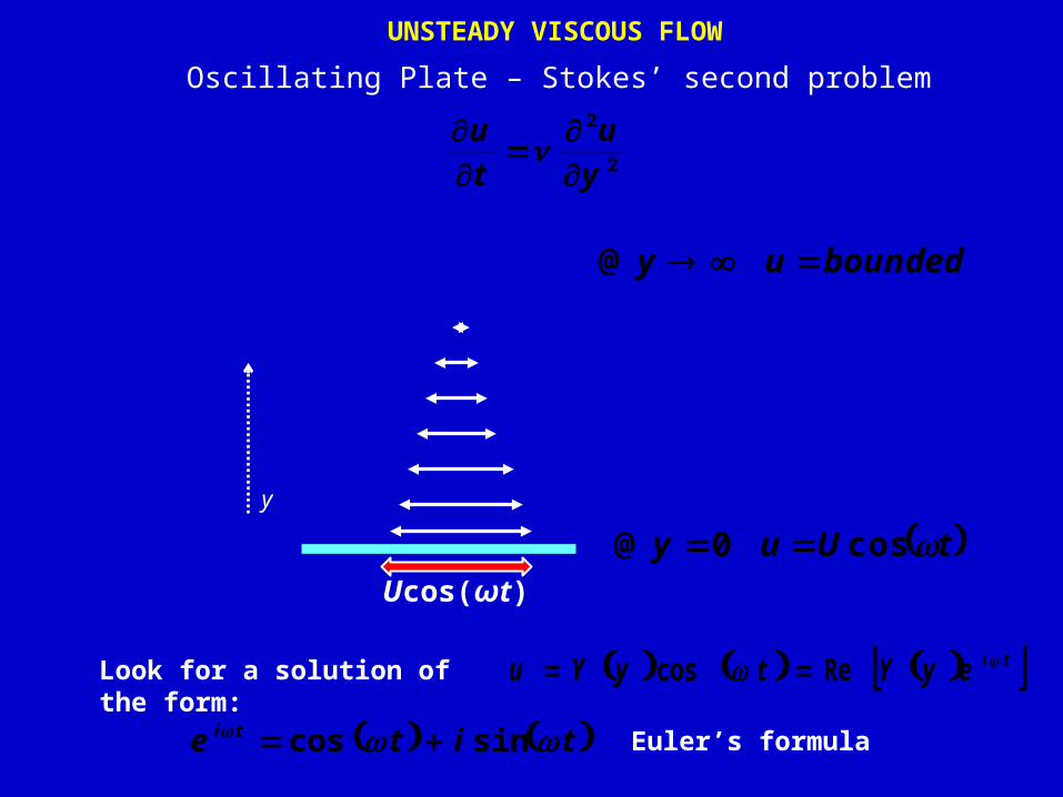
UNSTEADY VISCOUS FLOW
Oscillating Plate – Stokes’ second problem
tUuy cos0@
boundeduy @
Ucos(ωt)
y
Look for a solution of the form: tieyYtyYu Recos
tite ti sincos Euler’s formula

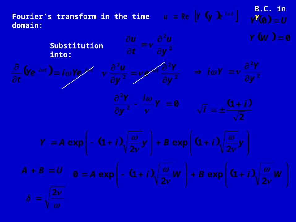
Fourier’s transform in the time domain: tieyYu Re 0YU
0Y
B.C. in Y
2
2
y
u
t
u
Substitution into:
titi YeiYet
2
2
y
YYi
2
2
2
2
y
Ye
y
u ti
02
2
Yi
y
Y
2
1 ii
yiByiAY
21exp
21exp
00 BY UAUY 0
yiUY
2
1exp

yiUY
2
1exp
y
tUeYeuy
ti cosRe
Most of the motion is confined to region within:
2
Ucos(ωt)
y
UUeUe
yy
37.0
@
1
UUeUeUe
yy
06.0
/4@
24

y
tUeuy
cos
2
2
y
u
t
u
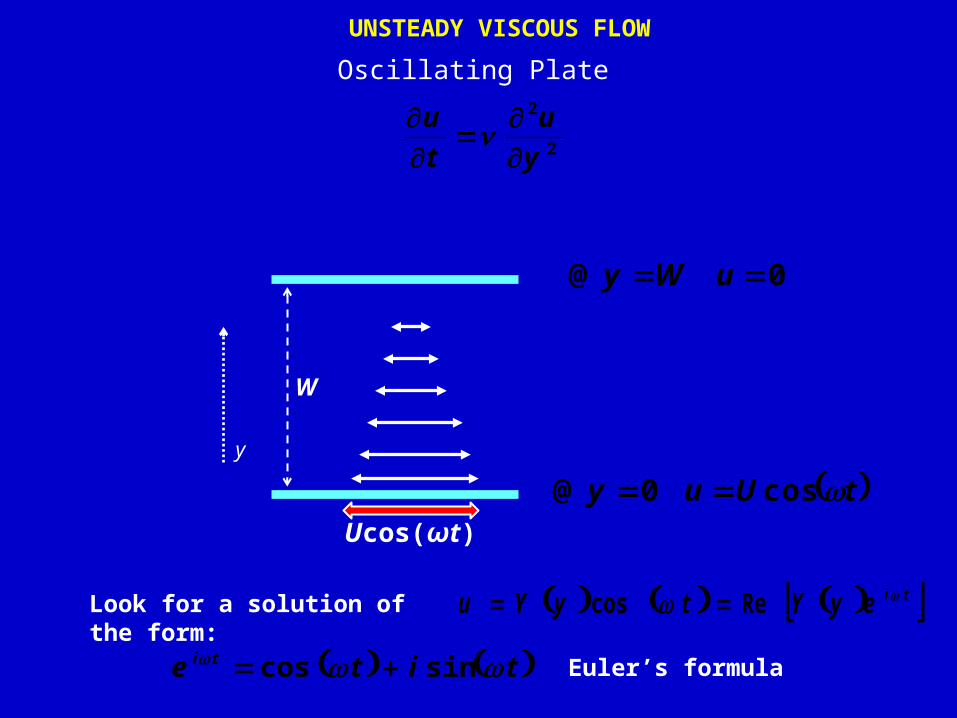
UNSTEADY VISCOUS FLOW
Oscillating Plate
tUuy cos0@
0@ uWy
Look for a solution of the form: tieyYtyYu Recos
tite ti sincos Euler’s formula
Ucos(ωt)
y
W
Fourier’s transform in the time domain: tieyYu Re UY 0
0WY
B.C. in Y
2
2
y
u
t
u
Substitution into:
titi YeiYet
2
2
y
YYi
2
2
2
2
y
Ye
y
u ti
02
2
Yi
y
Y
2
1 ii
yiByiAY
21exp
21exp
UBA
WiBWiA
21exp
21exp0
2
UBA
W
iW
i
BeAe11
0 sinh2 ee
sinh2
Ue
B
Wi 1
sinh21
eUA
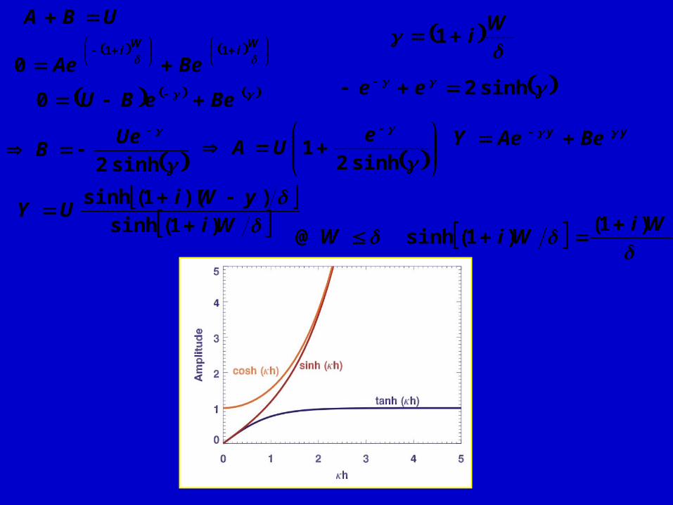
yy BeAeY
Wi
yWiUY
)1(sinh
))(1(sinh
Wi
WiW)1(
)1(sinh@
BeeBU 0

W
yU
W
yWUY 1
tW
yUu cos1
Wi
eWiW)1(
21)1(sinh@
yi
UY)1(
exp
Wi
yWiUY
)1(sinh
))(1(sinh
sinh2 ee Same solution as for unbounded oscillating plate

tW
yUu cos1


![Boundary layer Viscous Flow of Nanofluids and Heat ...€¦ · MHD steady flow of viscous nanofluid due to a rotating disk using HAM solutions. Kiran Kumar et al. [52] studied unsteady](https://cdn.vdocument.in/doc/165x107/5f35aad796ce023095738f65/boundary-layer-viscous-flow-of-nanofluids-and-heat-mhd-steady-flow-of-viscous.jpg)


