
Sandia is a multiprogram laboratory operated by Sandia Corporation, a Lockheed Martin Company,
for the United States Department of Energy’s National Nuclear Security Administration
under contract DE-AC04-94AL85000.
Validation & Verification and Uncertainty Quantification at Sandia
Brian M. Adams
Sandia National LaboratoriesOptimization and Uncertainty Quantification
July 18, 2008
Research Consortium for Multidisciplinary System Design Workshop
MIT, Boston, MA

Outline
•
Credible simulation and V&V•
Characterizing and propagating uncertainty for risk analysis and validation
•
Intro to aleatory
and epistemic UQ in DAKOTA•
Application examples:–
UQ for CMOS7 ViArray
UQ –
Sandia’s
QASPR program: computational model-
based system qualification
To be credible, simulations must be verified, validated with data, and deliver a best estimate of performance, together with its degree of variability or uncertainty.
Slide credits: Mike Eldred, Laura Swiler, Tony Giunta, Joe Castro, Genetha
Gray, Bill Oberkampf, Matt Kerschen, others

Insight from Computational Simulation
dHurricane Katrina: weather,
logistics, economics, human behavior
Electrical circuits: networks, PDEs, differential algebraic
equations (DAEs), E&M
Earth penetrator: nonlinear PDEs
with contact, transient analysis, material modeling
Micro-electro-mechanical systems (MEMS): quasi-
static nonlinear elasticity,
process modeling
Joint mechanics: system-
level FEA for component
assessment
Systems of systems analysis: multi-scale, multi-phenomenon

Credible Simulation
•
Ultimate purpose of modeling and simulation is (arguably) insight, prediction, and decision-making need credibility for intended application
•
Historically: primary focus on
modeling fidelity
Bill Oberkampf

Credible Simulation: V&V and UQ
Bill Oberkampf
Verification & Validation
•
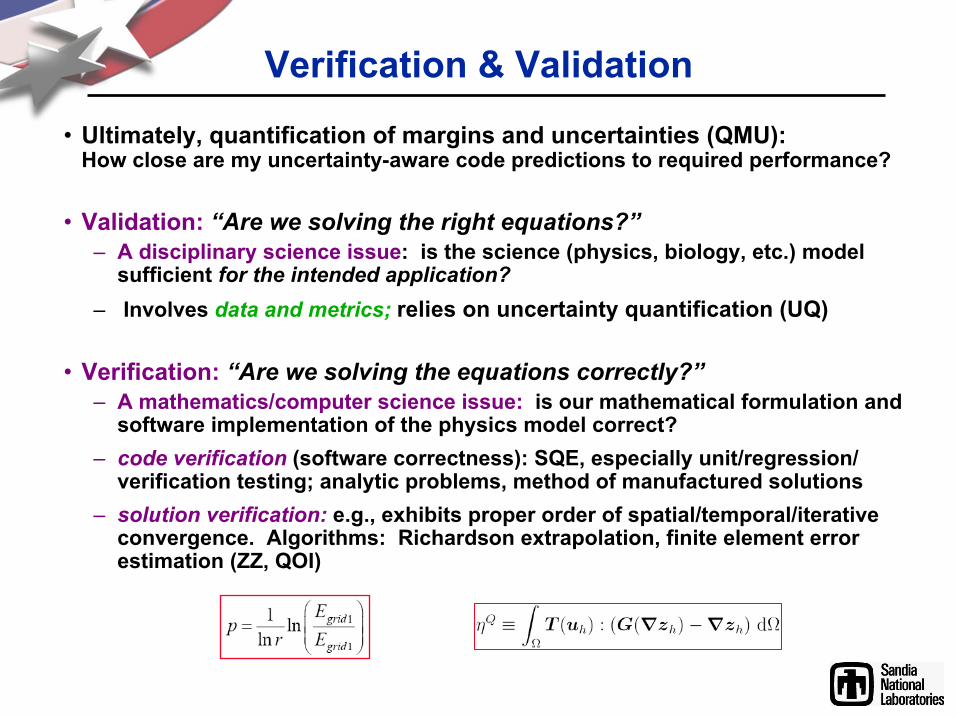
Ultimately, quantification of margins and uncertainties (QMU): How close are my uncertainty-aware code predictions to required performance?
•
Validation:
“Are we solving the right equations?”–
A disciplinary science issue: is the science (physics, biology, etc.) model sufficient for the intended application?
–
Involves data and metrics; relies on uncertainty quantification (UQ)
•
Verification:
“Are we solving the equations correctly?”–
A mathematics/computer science issue:
is our mathematical formulation and software implementation of the physics model correct?
–
code verification
(software correctness): SQE, especially unit/regression/ verification testing; analytic problems, method of manufactured solutions
–
solution verification:
e.g., exhibits proper order of spatial/temporal/iterative convergence. Algorithms: Richardson extrapolation, finite element error estimation (ZZ, QOI)

Algorithms for Computational Modeling & Simulation
System Design
Geometric Modeling
Meshing
Physics
Model Equations
Discretization
Partitioning and Mapping
Nonlinear solve
Linear solve
Time integration
Information Analysis & Validation
AdaptOptimization
and UQ
Improved design and understanding
Are you sure you don’t need verification?!

Hierarchical Validation Experiments (Abnormal Thermal Environment)
SubassembliesSubassemblies
Full SystemFull System
SeparableEffectsSeparableEffects
ComponentsComponents
Deployed SystemDeployed System
Bill Oberkampf
increasing complexity, few
er experiments
Validation:
“Are we solving the right equations?”
Based on experimental data and metrics, is the model sufficient for the intended application?
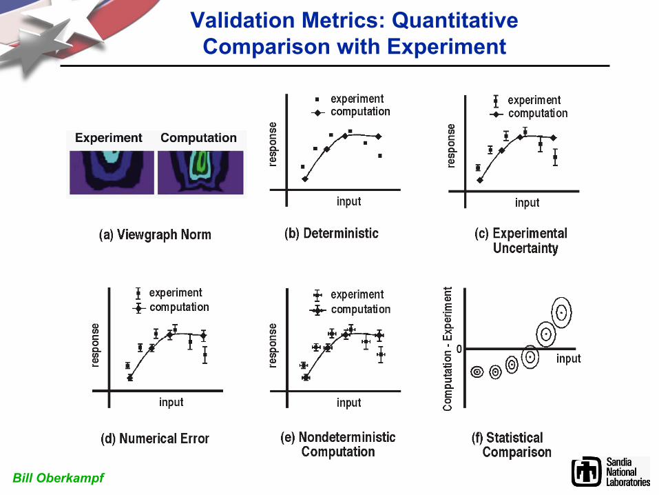
Validation Metrics: Quantitative Comparison with Experiment
Bill Oberkampf

Validation Metrics: Quantitative Comparison with Experiment
Bill Oberkampf
F in a l T e m p e ra tu re V a lu e s
0
1
2
3
4
5
Te m e pra ture [de g C]
% in
Bin
Test Data
Model Data
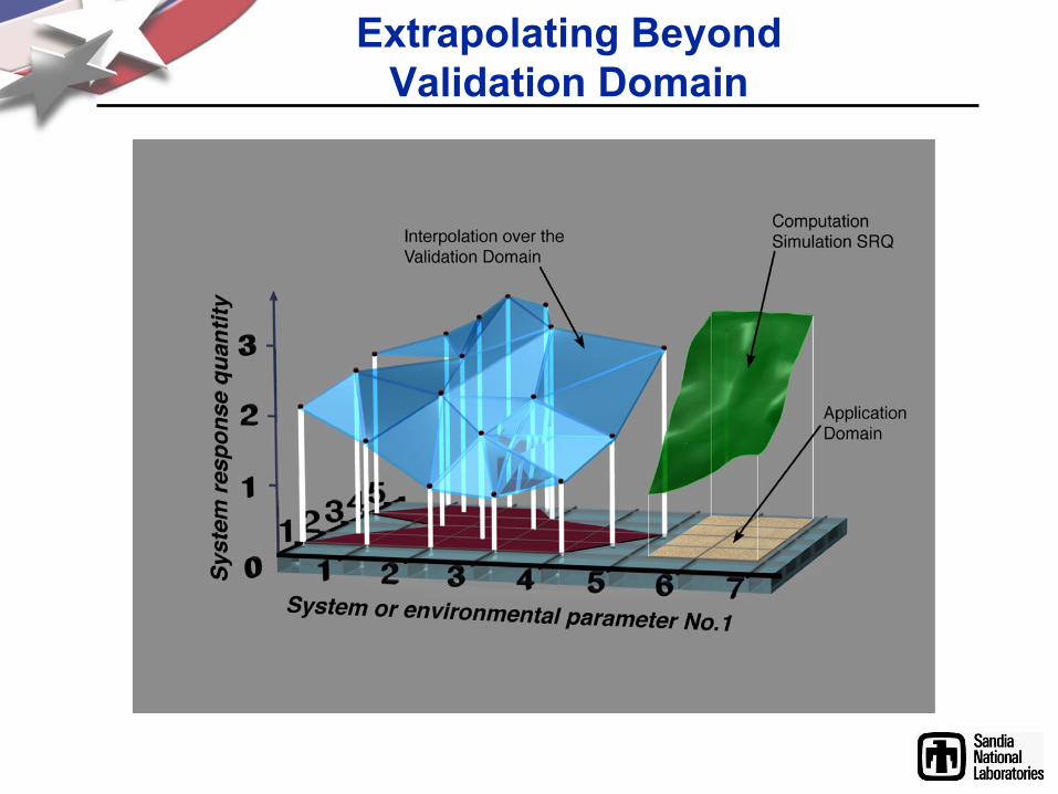
Extrapolating Beyond Validation Domain
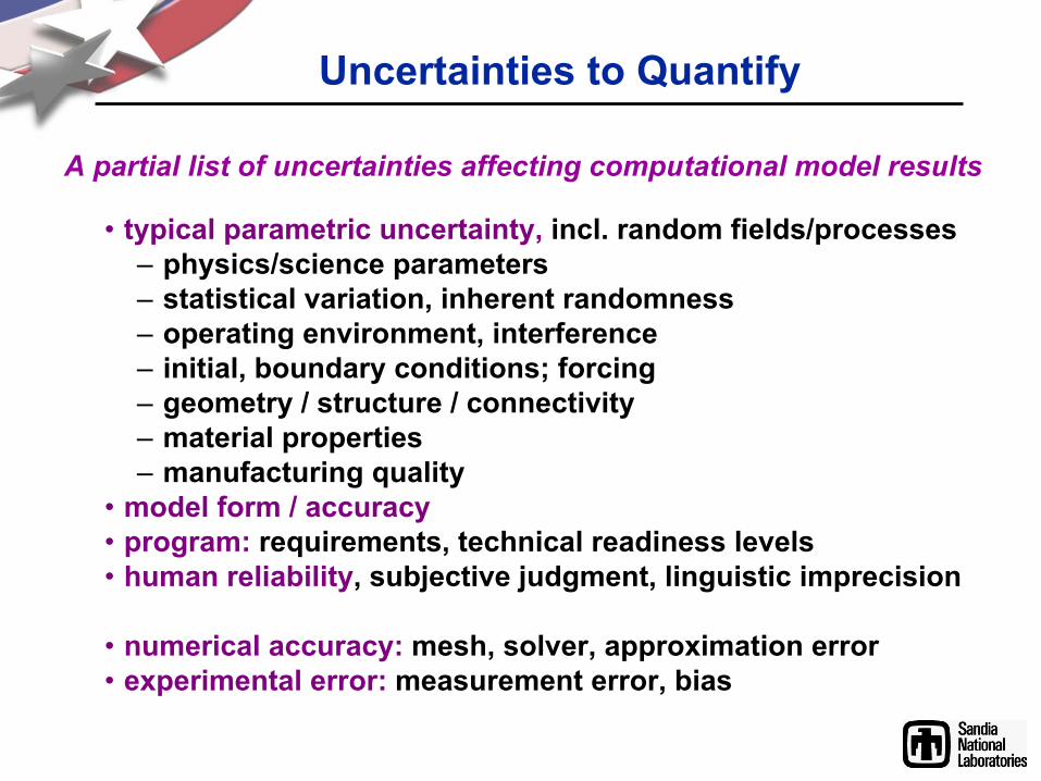
Uncertainties to Quantify
•
typical parametric uncertainty, incl. random fields/processes–
physics/science parameters–
statistical variation, inherent randomness–
operating environment, interference–
initial, boundary conditions; forcing–
geometry / structure / connectivity–
material properties–
manufacturing quality•
model form / accuracy•
program: requirements, technical readiness levels•
human reliability, subjective judgment, linguistic imprecision
•
numerical accuracy:
mesh, solver, approximation error•
experimental error:
measurement error, bias
A partial list of uncertainties affecting computational model results

•
A single optimal design or nominal performance prediction is often insufficient for –
decision making / trade-off assessment
–
validation with experimental data ensembles
•
Need to make risk-informed decisions, based on an assessment of uncertainty
Why Uncertainty Quantification?
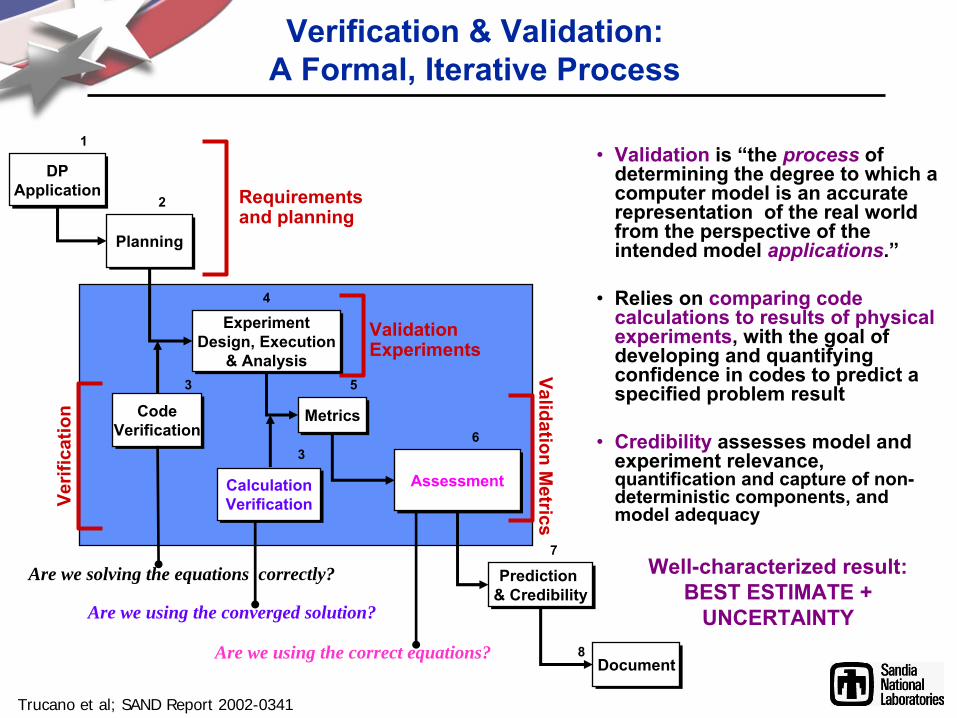
Verification & Validation: A Formal, Iterative Process
•
Validation
is “the process
of determining the degree to which a computer model is an accurate representation of the real world from the perspective of the intended model applications.”
•
Relies on comparing code calculations to results of physical experiments, with
the goal of developing and quantifying confidence in codes to predict a specified problem result
•
Credibility
assesses model and experiment relevance, quantification and capture of non-
deterministic components, and model adequacy
CodeVerification
CodeVerification
DPApplication
DPApplication
PlanningPlanning
ExperimentDesign, Execution
& Analysis
ExperimentDesign, Execution
& Analysis
MetricsMetrics
AssessmentAssessment
Prediction & CredibilityPrediction
& Credibility
DocumentDocument
CalculationVerificationCalculationVerification
1
7
6
5
2
4
3
3
8
Trucano et al; SAND Report 2002-0341
Requirements and planning
Validation Experiments
Verif
icat
ion
Validation Metrics
Are we solving the equations correctly?
Are we using the correct equations?
Are we using the converged solution?
Well-characterized result: BEST ESTIMATE +
UNCERTAINTY

Coverage Matrix Shows Code Features Exercised in Verification Tests
Sierra Capabilities (subset) SNL-Problem LANL-Problem
Matrix helps prioritize gaps, create new verification problems to fill most important, w.r.t. intended use.
Fills Gap
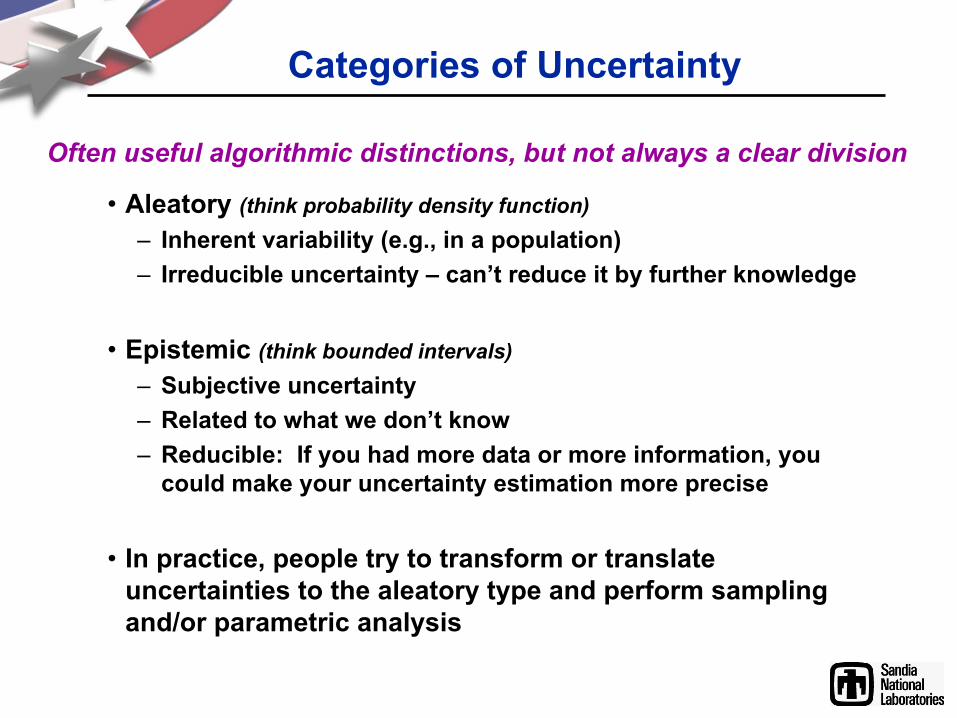
Categories of Uncertainty
•
Aleatory
(think probability density function)–
Inherent variability (e.g., in a population)–
Irreducible uncertainty –
can’t reduce it by further knowledge
•
Epistemic (think bounded intervals)–
Subjective uncertainty–
Related to what we don’t know–
Reducible: If you had more data or more information, you could make your uncertainty estimation more precise
•
In practice, people try to transform or translate uncertainties to the aleatory
type and perform sampling and/or parametric analysis
Often useful algorithmic distinctions, but not always a clear division

•
based on uncertain inputs, determine variance of outputs and probabilities of failure (reliability metrics)
•
identify parameter correlations/local sensitivities, robust optima
•
identify inputs whose variances contribute most to output variance (global sensitivity analysis)
•
quantify uncertainty when using calibrated model to predict
Uncertainty QuantificationForward propagation: quantify the effect that uncertain (nondeterministic) input variables have on model output
Potential Goals:
Input Variables u
(physics parameters, geometry, initial and boundary conditions)
Computational
Model
Variable Performance
Measures f(u)
(possibly given distributions)
Output Distributions
N samples
measure 1
measure 2
Model
Typical method: Monte Carlo Sampling
u1
u2
u3

Uncertainty Quantification Example
•
Device subject to heating
(experiment or computational simulation)
•
Uncertainty in composition/ environment (thermal conductivity, density, boundary), parameterized by u1
, …, uN•
Response temperature f(u)=T(u1
, …, uN
)
calculated by heat transfer code
Given distributions of u1
,…,uN
, UQ methods calculate statistical info on outputs:•
Probability distribution of temperatures•
Correlations (trends) and sensitivity of temperature•
Mean(T), StdDev(T), Probability(T
≥
Tcritical
)
Final Temperature Values
0
1
2
3
4
5
30 36 42 48 54 60 66 72 78 84
Temeprature [deg C]
% in
Bin

UQ: Sampling Methods
Given distributions
of u1
,…,uN
, UQ methods…
Final Temperature Values
0
1
2
3
4
5
30 36 42 48 54 60 66 72 78 84
Temeprature [deg C]
% in
Bin
Output Distributions
N samples
measure 1
measure 2
Model…calculate statistical info on outputs T(u1
,…,uN
)u1
u2
u3
• Monte Carlo sampling• Quasi-Monte Carlo• Centroidal
Voroni
Tessalation
(CVT)• Latin Hypercube sampling
0.2 0.2 0.2 0.2 0.2
A B C D−∞ ∞
0
0.2
0.4
0.6
0.8
1
A B C D−∞ ∞
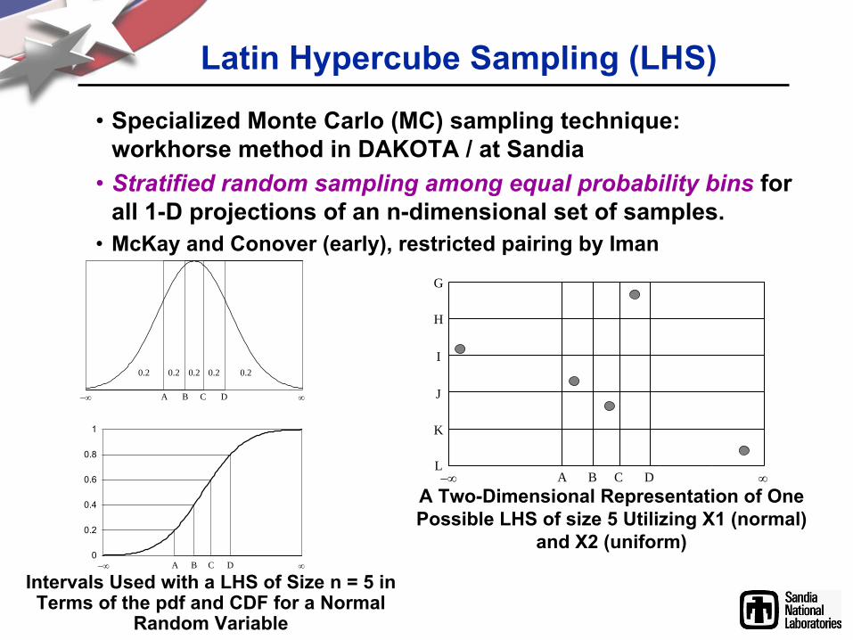
Latin Hypercube Sampling (LHS)
•
Specialized Monte Carlo (MC) sampling technique: workhorse method in DAKOTA / at Sandia
•
Stratified random sampling among equal probability bins
for all 1-D projections of an n-dimensional set of samples.
•
McKay and Conover (early), restricted pairing by Iman
A B C D
G
H
I
J
K
L−∞ ∞
Intervals Used with a LHS of Size n = 5 in Terms of the pdf
and CDF for a Normal Random Variable
A Two-Dimensional Representation of One Possible LHS of size 5 Utilizing X1 (normal)
and X2 (uniform)
Final Temperature Values
0
1
2
3
4
5
30 36 42 48 54 60 66 72 78 84
Temeprature [deg C]
% in
Bin
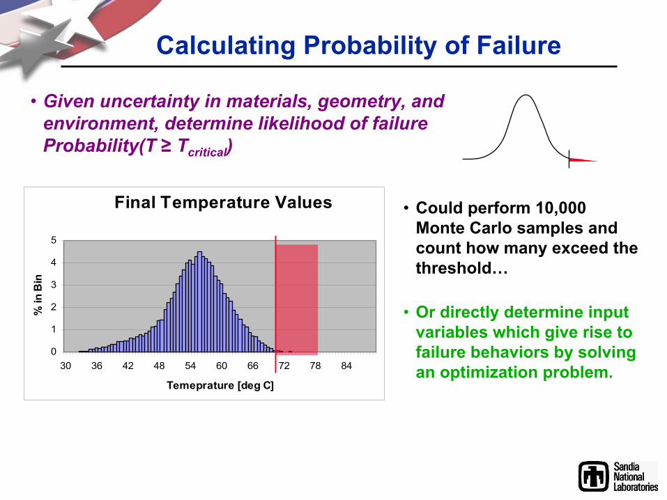
Calculating Probability of Failure
•
Given uncertainty in materials, geometry, and environment, determine likelihood of failure Probability(T
≥
Tcritical
)
•
Could perform 10,000 Monte Carlo samples and count how many exceed the threshold…
•
Or directly determine input variables which give rise to failure behaviors by solving an optimization problem.

Alternatives to Sampling
•
for a modest number of random variables, polynomial chaos expansions
may converge considerably faster to statistics of interest
•
if principal concern is with failure modes (tail probabilities),
consider global reliability methods
LHS sampling is robust, trusted, ubiquitous,
but advanced methods may offer advantages:
Hybrid
Surrogate Based
OptUnderUnc
Branch&Bound/PICO
Strategy
Optimization Uncertainty
2nd Order ProbabilityUncOfOptima
Pareto/Multi-Start
Upcoming (Mike): DAKOTA enables more efficient UQ by combining optimization, uncertainty analysis methods, and surrogate (meta-) modeling in a single framework.
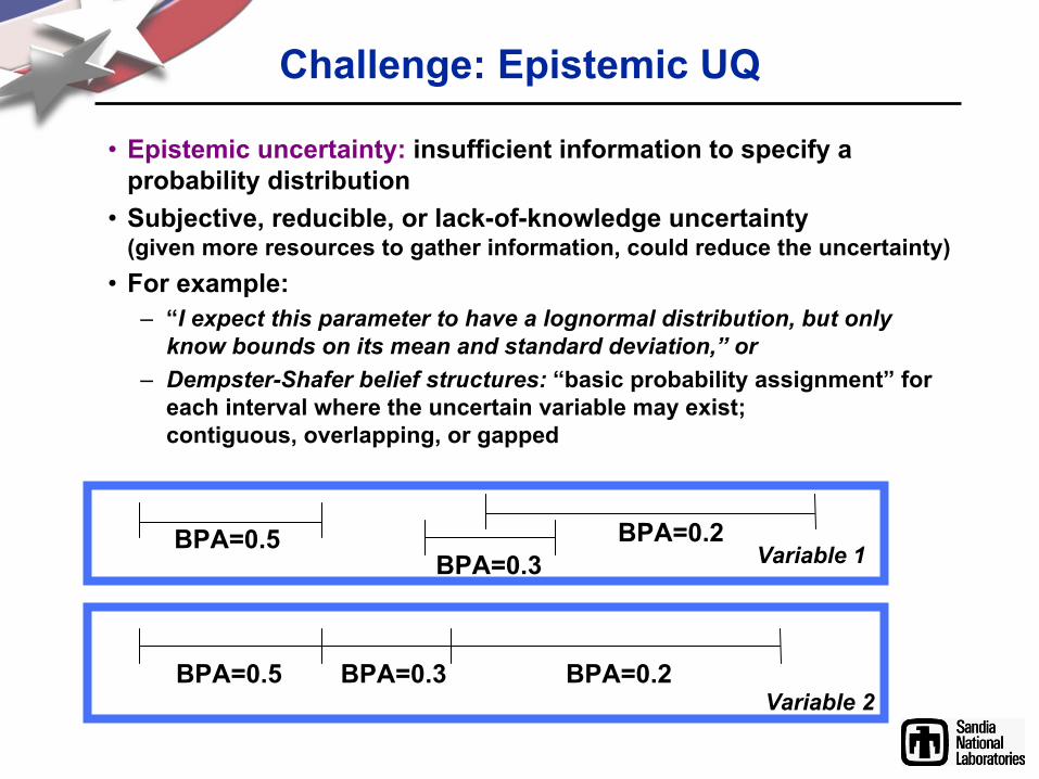
Challenge: Epistemic UQ
•
Epistemic uncertainty:
insufficient information to specify a probability distribution
•
Subjective, reducible, or lack-of-knowledge uncertainty (given more resources to gather information, could reduce the uncertainty)
•
For example:–
“I expect this parameter to have a lognormal distribution, but only know bounds on its mean and standard deviation,”
or–
Dempster-Shafer belief structures: “basic probability assignment”
for each interval where the uncertain variable may exist; contiguous, overlapping, or gapped
BPA=0.5 BPA=0.2BPA=0.3 Variable 1
BPA=0.5 BPA=0.2BPA=0.3Variable 2

Propagating Epistemic UQ
Second-order probability–
Two levels: distributions/intervals on distribution parameters
–
Outer level can be epistemic (e.g., interval)–
Inner level can be aleatory
(probability distrs)–
Strong regulatory history (NRC, WIPP).
Dempster-Shafer theory of evidence–
Basic probability assignment (interval-based)–
Solve opt. problems (currently sampling-based)
to compute belief/plausibility for output intervals
New
New

Circuit UQ Analysis
Use DAKOTA with Xyce
circuit simulator to perform pre-
fabrication uncertainty analysis of new CMOS7 ViArray
•
ViArray: generic ASIC implementation platform•
Target applications: guidance, satellite, command & control•
Assess voltage droop/spike during photocurrent event•
Consider effect of process variation in each ‘layer’
on supply voltages; representative distributions:
•
Truncated normals
used for METAL and VIA; truncated lognormals used for CONTACT and polyc.
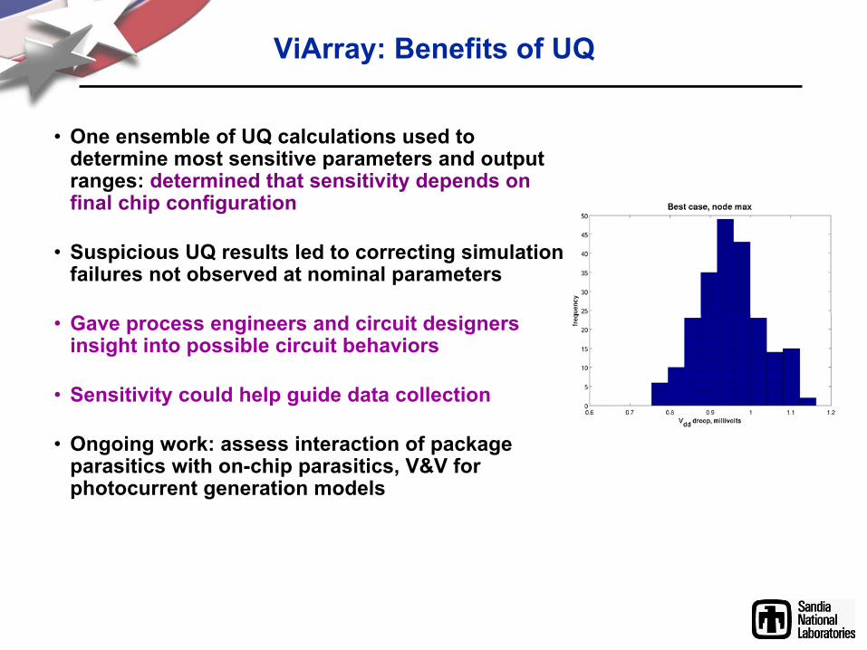
ViArray: Benefits of UQ
•
One ensemble of UQ calculations used to determine most sensitive parameters and output ranges: determined that sensitivity depends on final chip configuration
•
Suspicious UQ results led to correcting simulation failures not observed at nominal parameters
•
Gave process engineers and circuit designers insight into possible circuit behaviors
•
Sensitivity could help guide data collection
•
Ongoing work: assess interaction of package parasitics
with on-chip parasitics, V&V for photocurrent generation models
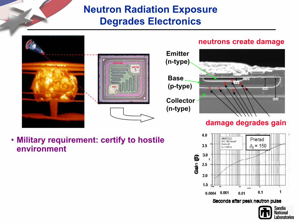
•
Military requirement: certify to hostile environment
neutrons create damageEmitter (n-type)
Base (p-type)
Collector (n-type)
xx
xxx
xx
damage degrades gain
Neutron Radiation Exposure Degrades Electronics

•
•
SPR dismantled end of FY06 to improve security posture
•
Military requirement: certify to hostile environment
neutrons create damageEmitter (n-type)
Base (p-type)
Collector (n-type)
xx
xxx
xx
damage degrades gain
Neutron Radiation Exposure Degrades Electronics
pass/fail
testing

quantified
uncertainty
•
•
SPR dismantled end of FY06 to improve security posture
•
Military requirement: certify to hostile environment
neutrons create damageEmitter (n-type)
Base (p-type)
Collector (n-type)
xx
xxx
xx
damage degrades gain
QASPR (Qualification Alternatives to Sandia Pulse Reactor) methodology will certify qualification via modeling &
simulation with quantified uncertainty
Neutron Radiation Exposure Degrades Electronics

UQ
M&SEC
select experiments in alternate facilities
γ,n – 100 mslong pulse
ion – 100 μsshort pulse
QASPR: Science-Based Engineering Methodology For Qualification
Risk InformedDecisions
QualificationEvidence2 4 6 8 10
time
0.2
0.4
0.6
0.8
1Current
uncertainty quantification
R2381.5k
Q28
MMBT2907
Q6MMBT2222
V23Vdc
M3
MTB30P06V
R239
1K
0
0
RF_PWR3_TXPA
Q62
BFS17A
DA_BATTERY3
R207
1k
R2361k
RL3
10
0
V8TD = 70msTF = 3nsTR = 3nsV1 = 3V2 = 0
Q63
MMBT2907
R24210
R251499
D50
MMSZ5236BT1
0
R204
4.99K
V1-8Vdc
FET_BIAS
VDD
R241
200
R240100
RF_PWR3_ENB_N
R206
1K
C15uF
R226
4.99k
R237
1k
R46
1k
V7TD = 0TF = 1msTR = 50msV1 = 0V2 = 10.8
0
C401uf
0
R210
10K
high performance, multi-fidelity, predictive computational modeling
validation

V&V for QASPR Components
•
Developing formal V&V plans
•
Each computational code subject to code and solution verification
•
UQ used to validate device model response against data ensembles
•
Ultimately systems (circuit) V&V for qualification

Device Prototype: UQ Extrapolation to SPR
•
Calibrated to other facilities, CHARON fills SPR gap
•
Uncertainty & bias characterized by 2 degrees of freedom–
facility multiplier–
device multiplier
•
Uncertainty quantified with D.O.E + statistical approach
End UQ Methodology Goal: Best Estimate + Uncertainty Prediction for SPR
Facility Multiplier, F
Device Multiplier, M
μM-MS
= 1.0
μF-SPR
= 1.0μF-ACR
= 0. 88
μM-FA
= 1.07
Model DevelopmentFacility Bias
BE+U Prediction
σF-SPR
Device Bias
σM-FA

+2σ
peak damage
-2σ
mean
Model Validation: Blind Prediction
UQ algorithms have a critical role in system validation
Transient Device Damage Response•
Fairchild response data within SPR hidden
•
First prototype
of the QASPR methodology (and real validation of the QASPR system)
•
Prediction + Uncertainty (+/-2σ
device and facility uncertainty)

Model Validation: Blind Prediction
UQ algorithms have a critical role in system validation
+/- 1-2% vertical error on experimental measurement
Transient Device Damage Response•
Fairchild response data within SPR hidden
•
First prototype
of the QASPR methodology (and real validation of the QASPR system)
•
Prediction + Uncertainty (+/-2σ
device and facility uncertainty)

Electrical Modeling Complexity
•
simple devices:
1 parameter, typically physical and measurable
•
e.g., resistor @ 100Ω
+/-
1%•
resistors, capacitors, inductors, voltage sources
Circuit Board
Large Digital Circuit(e.g., ASIC)
Sub-circuit (analog)
Single Device
device: 1 to 100s of params
sub-circuit: 10s to 100s of devices
ASIC: 1000s to millions of devices
•
complex devices:
many parameters, some physical, others “extracted”
(calibrated)•
multiple modes of operation•
e.g., zener
diode: 30 parameters, 3 bias states; many transistor models (forward, reverse, breakdown modes)
simulation tim
e grows exponentially
(G. Gray, M. M-C)
complex device models + replicates in circuits

UQ: Mitigate Explosion of Factors!
L
H
N
•
Consider bounding parameter sets?
•
Exploit natural hierarchy or network structure?
•
Use surrogate/macro-models as glue between levels?
•
Need approaches curbing the curse of dimensionality

Summary
•
Formal V&V process helps certify credible simulation
•
Uncertainty quantification algorithms are essential in validation and calibration under uncertainty
•
Complex, large-scale simulations demand research in advanced efficient UQ methods
Thank you for your [email protected]
http://www.sandia.gov/~briadam
To be credible, simulations must be verified, validated with data, and deliver a best estimate of performance, together with its degree of variability or uncertainty.


![Untitled Document [] · to IC Unless otherwise indicated, all limits are specified for VDD = +2.7V to +5.5V, VSS = GND, TA = 25 °C, VCM = VDD/2, RL = 100kΩ to VDD/2, and VOUT ~](https://cdn.vdocument.in/doc/165x107/5e7405a09fd2db4c0a486c73/untitled-document-to-ic-unless-otherwise-indicated-all-limits-are-specified.jpg)


