DP2016/07

New Zealand’s Experience with Changing its

Inflation Target and the Impact on Inflation

Expectations

Michelle Lewis and C. John McDermott

May 2016

JEL classification: E17, E31, E52, E58

www.rbnz.govt.nz

Discussion Paper Series

ISSN 1177-7567

DP2016/07

New Zealand’s Experience with Changing its Inflation

Target and the Impact on Inflation Expectations∗

Michelle Lewis and C. John McDermott†

Abstract

We document the experience of the Reserve Bank of New Zealand inchanging its inflation target, particularly the effects on inflation expectations.Firstly, the Reserve Bank of New Zealand’s DSGE model is used to highlightexpectation-formation in the transmission following a change in the inflationtarget. Secondly, a Nelson-Siegel model is used to combine a number of inflationexpectation surveys into a continuous curve where expectations can be plotted as afunction of the forecast horizon. Using estimates of long-run inflation expectationsderived from the Nelson-Siegel model, we find that numerical changes in theinflation target result in an immediate change in inflation expectations.

∗ The Reserve Bank of New Zealand’s discussion paper series is externally refereed. The viewsexpressed in this paper are those of the author(s) and do not necessarily reflect the viewsof the Reserve Bank of New Zealand. We are grateful to Punnoose Jacob, Gunes Kamber,Leo Krippner, Nick Sander and Jed Armstrong for assistance with this project. We arealso grateful to our colleagues at the Reserve Bank for their helpful comments and the twoanonymous referees for their helpful comments.† Michelle Lewis: Economics Department, Reserve Bank of New Zealand, 2 The Terrace, PO

Box 2498, Wellington, New Zealand. email address: michelle.lewis@rbnz.govt.nz. JohnMcDermott: Economics Department, Reserve Bank of New Zealand, 2 The Terrace, POBox 2498, Wellington, New Zealand. email address: John.McDermott@rbnz.govt.nzISSN 1177-7567 c©Reserve Bank of New Zealand

Non-technical Summary

We study the macroeconomic consequences of a change in the inflation target bythe central bank. New Zealand’s experience with changing the inflation targetmakes it a natural laboratory to pursue our objective. We document the variouschanges that have been made to the Policy Targets Agreement since it was firstintroduced in 1990 until the most recent change in 2012. Using the Reserve Bankof New Zealand’s macroeconomic model, NZSIM, we provide an illustration ofhow the macroeconomy responds to changes in the inflation target. A distinctivefeature of NZSIM is that it allows for different expectations formation, and hencewe are able to trace out the transmission channel from changing the inflation targetunder different assumptions for how inflation expectations are formed. Any changein target results in a corresponding change to inflation and inflation expectationsin the long run. There are no long run changes to any real variable, such as output,but there may be changes in the short run depending how expectations are formed.

We test how inflation expectations, across an array horizons, changed followingchanges to the Policy Targets Agreement. Using term structure modellingtechniques, we estimate inflation expectation curves based on survey measuresof inflation expectations that have horizons from 1 to 10 years ahead. We findevidence of expectation rigidities, where inflation expectations adjust adaptivelyto past inflation. However, inflation expectations adjusted immediately to the 2002change in the Policy Targets Agreement. Following the 50 basis point increase inthe mid-point of the inflation target range in 2002, inflation expectations increasedsignificantly at all horizons, with long-run inflation expectations immediatelyincreasing 19 basis points.

1

1 Introduction

The essential characteristic of an inflation targeting regime is an explicit andpublicly announced inflation target. The target needs to specify the index usedto measure inflation, the target level, the tolerance interval, the time frame overwhich the inflation target is to be met, and possible circumstances when temporarydeviations from the target are warranted.

Recently, there has developed a debate about the benefits and risks of changingan inflation target. One strand of the debate emphasises the risk of unanchoringinflation expectations, while another strand focuses on the likelihood of the centralbank hitting the Zero Lower Bound (ZLB). We contribute to this debate byquantifying the effects of changing the inflation target, in the context of NewZealand. Having changed its inflation target a number of times since 1990,New Zealand provides a natural laboratory to understand the macroeconomicconsequences of changing an inflation target.

As a first step, we use the official DSGE model (NZSIM) of the Reserve Bankof New Zealand to highlight the effects of changing the inflation target on keymacroeconomic variables. Subsequently, we determine the likelihood of hittingthe ZLB within the model environment. We highlight the pivotal role played byinflation expectations in determining the economy’s response to any change in theinflation target. In the empirical analysis that follows, we apply the Nelson-Siegelmodel on inflation expectations data in New Zealand to generate expectationscurves fitted over various time-horizons. Examining such curves enables us tounderstand how expectations have shifted in response to changes in the inflationtarget.

The simulation results from NZSIM show that when inflation expectations adjustslowly to changes in the inflation target, there are short-run effects on realvariables. In contrast, when inflation expectations adjust rationally to changesin the inflation target, there are no short-run effects on real variables. In addition,for any given level of the inflation target, the probability of hitting the ZLB ishigher when inflation expectations are formed adaptively relative to when theyare formed rationally.

The results from the Nelson-Siegel model suggest that changes to the inflationtarget change inflation expectations significantly. In particular, long-run inflationexpectations change in response to numerical changes to the inflation target.

As noted earlier, we focus on quantifying the effects of changing an inflationtarget. We do not examine the desirability of changing the inflation target, whichhas been the focus of a recent literature. Orphanides and Williams (2005) show

2

that uncertainty about an inflation target worsens macroeconomic performance.Recently, Blanchard, Dell’Ariccia, and Mauro (2010), controversially, suggestedthat to reduce the risk of deflation, developed countries should increase theirinflation targets from the current level of about 2 percent to 4 percent. Theargument was that such a change would reduce the likelihood of central bankshitting the ZLB and thus provide more scope for monetary policy in seriousdownturns. However, this suggestion was criticized by Buiter (2010) as being‘the first step on the slippery slope of inflation creep’. Buiter is reflecting thepolitical economy concerns that raising the inflation target will reduce centralbanks’ credibility and lead to inflation expectations becoming unanchored. Incontrast, Granville (2013) argues that having an unrealistic target band couldresult in ‘negative consequences such as a political backlash against the IT[Inflation Targeting] regime’.

Clearly there is a need to be cautious about making changes to the inflationtarget but there may well be circumstances when a change to an inflation targetis warranted. Quantitative estimates of the impact of variations in the inflationtarget, such as those presented in this paper, are useful in any assessment of sucha significant institutional change.

The rest of the paper is set out as follows. We provide a condensed account of NewZealand’s experience of making changes to its inflation targeting regime in section2. The Reserve Bank’s DSGE model is used in section 3 to highlight the responseof macroeconomic variables to a change in the inflation target. In addition, wealso calculate the probability of being at the ZLB within this model environment.In section 4, we empirically assess the response of expectations to changes in theinflation target. Section 5 concludes.

2 Changes to the Inflation Target

The details of New Zealand’s inflation targeting regime have changed considerablysince it was introduced in the first Policy Targets Agreement (PTA) signed by theMinister of Finance and the Governor on 2 March 1990. The changes evolved withexperience and have reflected the growing international consensus for the need ofan inflation targeting regime to be flexible. The changes over time have been toall parameters of the regime, including: the numerical values of the target ceilingand floor (and by implication the mid-point of the target band), the measure of

3

inflation, and the timeframe in which the inflation target was to be met.1

Figure 1 shows inflation in New Zealand since the start of inflation targeting, asmeasured by the official CPI inflation, CPIX inflation (official CPI excluding someitems), and underlying inflation (a definition introduced by the Reserve Bank inorder to exclude some items). The grey area on the figure shows the target rangefor inflation over time and the black line indicates the introduction of the explicitmidpoint of the target range.

Below we provide our condensed account of New Zealand’s experience withchanging its inflation target. This account focuses on five changes to the PTA:the start of inflation targeting in 1990, an increase of the target ceiling in 1996,the introduction of secondary objectives in 1999, an increase of the target floor in2002, and the introduction of an explicit reference to a midpoint in 2012. Otherchanges to the PTA in 1992, 1997, 2007, and 2008 did not alter the parameters ofthe inflation targeting regime and so are not discussed.

Figure 1: New Zealand’s Inflation Target

-1

0

1

2

3

4

5

6

7

8

1990 1994 1998 2002 2006 2010 2014

Per

cent

-1

0

1

2

3

4

5

6

7

8% %

Official CPIinflation

Targetband

CPIX

Underlyinginflation

Note: New Zealand’s inflation target and CPI inflation since the start of the inflation targeting

regime. The grey band reflects the inflation target range over time and the black line represents

the increased focus on the midpoint since September 2012. The dashed blue line, CPIX, is the

official CPI inflation measure excluding some items.

1 The various vintages of the PTA can be viewed at http:/www.rbnz.govt.nz/monetary policy/policy targets agreement/. Further details on the history of the PTA can be found in ReserveBank of New Zealand (2000, 2007).

4

2.1 A time varying start before settling on 0 to 2 percent

The first numerical target for inflation in New Zealand was specified as an annualinflation rate in the range of 0 to 2 percent of an adjusted consumer price index.The adjustment to the headline CPI was required because, at the time, the Bankbelieved that consumer price inflation would be better represented by an index inwhich housing costs and mortgage interest rates were replaced by a measure of therental value of a owner-occupied house.

The adjustment was made to avoid the problem of targeting a measure of inflationthat includes interest rates. If inflation was too high, then interest rates wouldneed to be increased to moderate inflationary pressures, but inflation may actuallyincrease further because of the interest rate component. Moreover, the Bank could,in the short run, hit its inflation target by moving interest rates in the oppositedirection to what would be required for medium-term price stability.

When the target was introduced, the PTA specified a transitional period for theBank to bring inflation down to its target. The PTA indicated that the Bankshould implement monetary policy to ‘achieve a steady reduction in the annualrate of inflation through the period to December 1992’. The first Monetary PolicyStatement (MPS), issued in April 1990, made the idea of a steady reduction morespecific by providing the target for annual increases in the CPI of:

• 3-5 percent for the year to December 1990;• 1-.5-3.5 percent for the year to December 1991; and• 0-2 percent for the year to December 1992.

After December 1992 the inflation target was specified as 0 to 2 percent. Thetargeted measure of inflation evolved into what became known as ‘underlying’inflation. This measure started with the official Consumer Price Inflation (CPI),deducted interest rates and sometimes deducted other items, such as: significantchanges in the terms of trade, significant change in indirect tax rates (such as theGoods and Services Tax), and significant price level changes arising from changesto government or local authority levies.

2.2 Target band widened to 0 to 3 percent

On 10 December 1996, the inflation target band was widened to 0 to 3 percent(from 0 to 2 percent). The official measure of inflation, the CPI, was still not usedas the target measure. Instead, the Bank published its measure of ‘underlying’inflation. While this approach was consistent with the intent of the PTA, there wasa significant problem with the Bank calculating its own target measure. This left

5

a perception, in some quarters, that the Bank was potentially able to manipulatethe measure of inflation on which the Bank’s, and the Governor’s, performancewas judged.

By December 1997 the Bank chose to target Statistics New Zealand’s publishedCPI excluding credit services (denoted CPIX) rather than the Bank’s measure ofunderlying inflation. Following a review by Statistics New Zealand of the contentand calculation of the CPI in June 1999, mortgage interest rates were excludedfrom the official calculation and so the Bank started targeting the CPI all groupsmeasure produced by Statistics New Zealand. Since the Bank no longer had tomake technical adjustments to the CPI, public communication about inflationbecame far easier.

2.3 Introducing secondary objectives

In December 1999, secondary objectives were added to the PTA to increase theflexibility of the framework. Clause 4(b) of the PTA now stated that:

“In pursuing its price stability objective, the Bank shall implement monetarypolicy in a sustainable, consistent and transparent manner and shall seek to avoidunnecessary instability in output, interest rates and the exchange rate.”

The desire to avoid unnecessary instability in a set of macroeconomic variablesformalised the recognition that attempting to use monetary policy to offsetshort-term impacts on inflation would typically aggravate any financial marketturbulence or economic volatility. The implication for the practice of monetarypolicy is that interest rates would be adjusted more gradually than otherwise.2

The explicit mention of financial variables, such as interest rates and exchangerates, is unusual by international standards, especially since it is sometimesnecessary to move interest rates aggressively to stabilize output and inflation. Forexample, it was necessary to reduce the Official Cash Rate (OCR) by 575 basispoints in 2008/09 to help stop a downturn in output and inflation. Nevertheless,in more normal times, it is generally desirable for interest rates to be stable tofacilitate business and household investment decisions. Also, unnecessarily volatileexchange rates have the potential to adversely affect profits in the export andimport-competing sectors and discourage firms from investing in these sectors ofthe economy.

2 To a degree, these changes to the PTA cemented what was already being practised. Realeconomy considerations are always present when thinking about how to set monetary policyto achieve an inflation target. For further details on the Bank’s contemporary interpretationsof Clause 4(b) of the PTA, see Hunt (2004) and Bollard and Karagedikli (2006).

6

2.4 Target band narrowed to 1 to 3 percent but moreflexibility allowed over the target horizon

In September 2002, a new PTA was introduced that changed the inflation targetin a number of dimensions, including:

• the target floor was raised from 0 to 1 percent, while the targetceiling remained at 3 percent; and

• the target horizon was redefined to ‘future CPI inflationoutcomes... on average over the medium term’.

This numerical change to the band both narrowed the tolerance interval for whatcould be deemed satisfactory inflation outcomes and raised the midpoint of thetarget band, making it the second time the value of the midpoint has been changed.In addition, the timeframe required to meet this target was made more flexible.The PTA required the Bank to take a forward-looking, medium-term approach toachieving its target, firmly embedding the idea of a flexible framework.

The Bank has interpreted this target to mean that the Bank should set monetarypolicy so that in response to deviations of inflation from target, and in the absenceof significant unforeseen events, inflation will be back with the target band in thelatter half of a three-year horizon.3 Moreover, it was thought that if inflationprojections were too close to the edge of the target band, then there was a risk ofbeing pushed outside the band from even minor surprises.4 Therefore, the Bankwould set policy so that inflation would gradually move toward the centre of theband and settle ’comfortably’ inside the 1 to 3 percent band.

The specification of the target in terms of ‘future CPI inflation outcomes ... onaverage over the medium term’ allowed the Bank more leeway in responding toone-off deviations that would not be expected to disturb the medium-term trendof inflation. This new target gave the Bank a framework in which to clearlycommunicate its judgement about whether deviations of inflation from target weretemporary or not. Clearer communication provided the public with informationthat any deviation did not signal the existence of an ongoing inflationary problem.A ’medium-term’ target horizon depends on the circumstances at the time and, inparticular, how well inflation expectations are anchored to the target.

3 The intention to bring inflation back to a comfortable part of the target band in a specifiedtimeframe following any deviation from target was stated publicly in Bollard (2002, 2008).

4 Hargreaves (2002) conducts simulation experiments to show how inflation variability wouldchange if the Bank used the target band as a ‘zone of inaction’. That is, monetary policydoes not respond when inflation is inside the target band. He finds that such a strategy wouldmake breaches of the target band much more likely.

7

2.5 Explicit reference to the 2 percent midpoint

In September 2012, an explicit reference to the midpoint of the target band wasadded to the PTA. Clause 2(b) of the PTA adds ‘a focus on keeping future averageinflation near the 2 percent target midpoint’. This addition was motivated bythe desire to anchor inflation expectations more firmly to 2 percent (see Kendalland Ng, 2013). The explicit focus on the 2 percent midpoint could be viewedas communicating that the edges of the target band are less tolerable than thecentre of the band. However, as noted above, even prior to the explicit mentionof a midpoint, monetary policy was always set with the aim of moving inflationgradually to the centre of the target band. The addition is perhaps better seenas formalising the flexible approach to inflation targeting that is practiced in NewZealand.

3 Changing the Inflation Target in NZSIM

The most memorable changes to the inflation target have been those that alteredthe midpoint of the target range. Here we demonstrate that the macroeconomicconsequences of changing the midpoint of the inflation target depend cruciallyon inflation expectations. First, we examine the macroeconomic impact of achange in the inflation target under both adaptively and rationally formed inflationexpectations. This exercise illustrates model dynamics under each assumption,which are well-established in the literature, and sets the scene for the empiricalresults in section 4. Second, we calculate the probability of hitting the ZLB as afunction of the inflation target, again under both adaptively and rationally formedinflation expectations. This exercise allows us to assess different inflation targets,in terms of the risk that policy hits the zero lower bound in a typical businesscycle.

3.1 Predicted effects of target changes in NZSIM

To help inform us about the macroeconomic impacts of changing the inflationtarget we can look at simulations from macroeconomic models. Here, we use theReserve Bank of New Zealand’s estimated dynamic stochastic general equilibrium(DSGE), referred to as NZSIM. For a description of the underlying structure of

8

NZSIM and model equations see Kamber et al (2015).5

NZSIM is used in the policy formation process at the Bank and reflects institutionalviews on the key monetary policy transmission channels and business cycledynamics. At the core of NZSIM is a conventional small open economy NewKeynesian model, with three types of optimising agents: households, domesticfirms, and import distributing firms. The central bank targets inflation to diminishthe inefficiencies associated with the presence of sticky nominal prices. Themodel is kept parsimonious to ensure it is transparent and easy to communicate,while the core structure gives confidence in providing policy analysis through amodel-consistent framework.

A key feature in NZSIM that makes it suitable for our analysis is that itallows inflation expectations to potentially be adaptive. In particular, inflationexpectations are a convex combination of its lagged value and the rationalexpectation. The motivation for using the adaptive expectations process comes,firstly, from empirical tests for New Zealand, which suggest inflation expectationsare likely to be adaptive.6 Secondly, adaptive expectations provide a better fitto the data when using inflation expectations as an observable series. Manyconventional models used at other central banks, and in the literature, use rationalexpectations and do not usually use inflation expectations as an observable seriesin the estimation.7 Using NZSIM in this exercise means we are able to assess theeffects from changing the inflation target in both environments, when inflationexpectations are formed rationally and when they are formed adaptively. Othermodels estimated for New Zealand use purely rational expectation formation andare hence less suitable for our purpose (for example, Jacob and Munro 2016,Justiniano and Preston 2010, and Kam, Lees and Liu 2009).

The monetary policy rule we use in the current exercise is

it = φiit−1 + (1− φi){πt + φπ(Etπt+1 − πt + φyyt}+ εit (1)

5 Kamber et al (2015) provide a technical description of the NZSIM model that is based on astandard open economy dynamic stochastic general equilibrium. The version of NZSIM usedin the forecasting process, and in this paper, also includes additional semi-structural auxiliaryequations. The equations are in the Appendix.

6 See, for example, Karagedikli and McDermott (2016), Kamber et al. 2015, Hargreaves, Kite,and Hodgetts (2006), and Razzak (1997) for discussions on modelling inflation expectationsin New Zealand.

7 For a discussion of the Bank of England’s core DSGE model, COMPASS, that uses rationalexpectations and an alternative model MAPS for different expectation formation processessee Burgess et al (2013). For a discussion on the Bank of Canada’s TOTEM and TOTEM IImodels, which uses forward-looking and rule-of-thumb expectations, see Dorich et al (2013).

9

where it is the policy interest rate, Etπt+ 1 is the rational expectations of inflationat time t+ 1 formed at time t, yt the output gap at time t, εit is a monetary policyshock and πt is the inflation target. Our experiment is performed by makingpermanent changes to πt.

Inflation expectations are formed according to the following process

πet,t+1 = ρ1πet−1,t + (1− ρ1)[ρ2Etπt+1 + (1− ρ2)πt−1] (2)

where πet,t+1 is the level of expectations of inflation in period t+ 1 held by businessand household agents at time t and πt−1 is the level of inflation at time t−1. Thisapproach of how expectations are formed is applied consistently to non-tradableinflation, tradable inflation and wage inflation in the model.

Impulse responses for a one percentage point increase in the inflation target arecomputed under two scenarios: (i) inflation expectations follow an adaptive processwith ρ1 = 0.92 and ρ2 = 0, and (ii) inflation expectations are fully rational withρ1 = 0 and ρ2 = 1. The parameter values used to generate adaptive expectationsare the same values used in the version of NZSIM that is used to produce theforecasts in the Monetary Policy Statement. Qualitatively similar results canbe obtained for a wide range of values of ρ1 = 0. To illustrate the role of theparameters, as ρ1 = 0 falls and ρ2 = 0 increases, agents become more forwardlooking and the persistence of variables, particularly price variables, falls. AsKamber et al. (2015) explain, the lower persistence occurs because agents placeless emphasis on past expectations of future marginal costs and more emphasis onfuture expectations, which makes prices less sticky.8

In the adaptive expectations scenario any change of the inflation target changesinflation expectations slowly, requiring monetary policy to be more aggressiveto ensure actual inflation converges to target. Under the rational expectationsscenario inflation expectations adjust immediately to changes in the inflationtarget. For these scenarios the target is taken to be the midpoint of the toleranceinterval.

Figure 2 shows the outcomes of these simulations for a range of macroeconomic

8 The parameter ρ1 needs to be high but less than unity under adaptive expectations. Thevalue of 0.92 was chosen because that is the estimated value in NZSIM.

10

variables for a one percentage point increase in the inflation target.9 The solid linein the figure reports the results from the adaptive inflation expectations scenariowhile the dashed lines show the results from the rational expectations scenario.

When inflation expectations adjust slowly to information about an increase in theinflation target, nominal interest rates need to be lowered immediately in orderto generate a positive output gap to move inflation to the new target. Even afterinflation reaches the new target there is still a need to run a positive output gapfor a lengthy period to force inflation expectations to adjust upward to the newtarget. As inflation expectations gradually increase, nominal interest rates needto increase, ultimately to one percentage point higher than the neutral level underthe old inflation target. The temporary boost to the level of GDP is composedof increases in consumption, investment and exports. However, consumption andimports later fall below their initial level but the output gap remains positive.This shift away from consumption toward net exports reflects a real exchange ratedepreciation.

In contrast, under the rational expectations scenario there is virtually no boostto the level of GDP while consumption falls temporarily, offsetting the smalltemporary increases in investment and net exports. In both scenarios, inflationincreases permanently by exactly the amount of the increase in the inflationtarget. In the long run, inflation expectations and nominal interest rates increasepermanently so that the long-run level of real interest rates is constant.

9 These experiments are conducted under the assumption that only small changes in theinflation target are considered, so that the model’s structure can be assumed constant despitethe change in institutional settings (i.e. the Lucas critique is not an issue). If changes to theinflation target were large enough we may see threshold effects where the private sector, inorder to avoid the costs of inflation, engages in speculative activity rather than productiveactivity, reducing the economy’s supply potential. For evidence of how inflation beyond acertain threshold reduces growth, see Khan and Senhadji (2001).

11

Figure 2: Effect of an inflation target increase in selected variables in NZSIM

0 20 40−5

0

5GDP

0 20 40−2

0

2

4Consumption

0 20 40−10

0

10

20Investment

0 20 400

1

2

3Exports

0 20 40−2

0

2Imports

0 20 400

0.5

1

1.5Inflation

0 20 40−1

0

1

2Interest Rates

0 20 40−20

−10

0

10Real Exchange Rate

0 20 40−1

0

1

2Inflation Expectations

Solid: Benchmark NZSIM model, where inflation expectations are adaptive; dashed: NZSIM

model with rational expectations. Note: a fall in the exchange rate denotes a depreciation

3.2 Avoiding the Zero Lower Bound

As noted in the introduction, one of the motivations posited by some authorsfor increasing the inflation target is to reduce the likelihood of hitting the zerolower bound (ZLB). A higher target results in both trend inflation being furtherfrom zero and trend nominal interest rates being further from zero. Higher trendnominal interest rates provide more scope for monetary policy to deal with adverseshocks. We use NZSIM to determine the probability of hitting the ZLB and stayingthere for a significant period. In this exercise we focus on a period of five quarterswhich is close to the typical length of a New Zealand recession.10 In particular,we calculate what shocks would be required to keep interest rates at the ZLB forfive consecutive quarters and the probabilities of those shocks occurring over abusiness cycle.

Intuitively, we impose the result that interest rates are at the ZLB for fiveconsecutive quarters and calculate the combination of shocks in NZSIM that wouldbe most consistent with this outcome. For each of the shocks we then calculate a

10 See Hall and McDermott (2009, 2011 and 2015) for evidence on the New Zealand businesscycle. The average duration of the nine recessions since 1947 is 4.2 quarters with a standarddeviation of 1.6. The last recession lasted 5 quarters from December 2007 to March 2009.

12

metric of its ‘implausibility’. An ’implausibility index’ of the ZLB event is thenthe average of the ‘implausibility’ of all the shocks and the probability of being atthe ZLB for five quarters is simply one minus the ‘implausibility index’.11

The implausibility index we use was introduced by Doan, Litterman and Sims(1983). Suppose that forcing the model to be at the ZLB for h quarters requiresthe following future values for the kth shock to be set to εkt+1, ..., ε

kt+h where k is

an index of shocks in NZSIM. The Waggoner and Zha (1999) algorithm is usedto compute the values εkt+1, ..., ε

kt+h for k = 1, ..., K, where K is the total number

of shocks used from the model. There are 21 shocks in NZSIM and all of theseshocks are used in the exercise.

To select the shocks in this exercise we use the Waggoner-Zha algorithm, which isa common and agnostic approach for adding judgement in structural models. Inparticular, the algorithm determines the combination of shocks with the smallestvariances that are consistent with the conditional forecast. From a probabilisticpoint of view, the most likely sequence of shocks is chosen, given the structure ofthe model and its parameterisation. The Implausibility index then evaluates thevariance of the shocks used, comparing the size of the shocks used to generate thescenario to what has been experienced in history.

The implausibility index for h horizons is then given by

Ih =1

K.h

K∑k=1

h∑i=1

(ε̂kt+i)2

σ2k

(3)

where σ2k is the historical variance of the kth shock. If we need large values of

ε̂kt+i relative to the variance σ2k to generate the ZLB outcome then that outcome

would seem to be implausible, hence the name of the index. We can convert thisindex into a probability of being at the ZLB for h quarters using the cumulativedistribution function of a half normal random variable with unit variance. That is

Pr(ZLB, h) = 1−∫ Ih

0

√2

πexp

(−1

2x2)dx. (4)

11 The concept of an implausibility index can seem unintuitive. An alternative way of expressingthe concept follows. In this exercise, starting from equilibrium, we generate a scenario whereinterest rates are at the zero lower bound for five consecutive quarters using all the shocksin the model. The shocks used to generate this scenario are compared to history to informus whether the required shocks are ‘plausible’ given what we have observed in history. Thisexercise is done for different inflation targets.

13

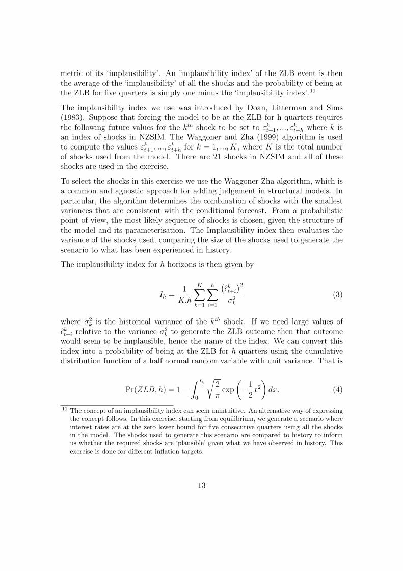
Figure 3 shows the probability of being at the ZLB for five quarters as a functionof the inflation target assuming the neutral real interest rate is 2.5 percent.12 Inthis exercise, under rational expectations the probability of being at the ZLB forfive consecutive quarters for any non-negative inflation target is zero.

In contrast, when expectations are adaptive then there is a possibility of beingstuck at the ZLB. The probability of being at the ZLB for five quarters when theinflation target is zero is 0.29 and steadily declines as the inflation target increases.The midpoint of the original 0 to 2 percent target and the midpoint of the 19960 to 3 percent target produce probabilities of being at the ZLB for 5 quarters of0.12 and 0.05, respectively. With the current mid-point of the target at 2 percent,the probability of being at the ZLB for 5 quarters is 0.02. This indicates that thepotential gains from increasing the target above 2 percent are likely to be trivial.13

To generate a ZLB outcome in NZSIM with adaptive expectations the Waggonerand Zha algorithm requires four large shocks, two moderate shocks, and theremainder of the shocks are very small. The large shocks that are doing mostof the work are the inflation expectations, migration, monetary policy and retailinterest rate shocks. Exchange rate and consumption shocks are also required butthese tend to be moderate on average.

12 The neutral real interest rate chosen here is the same value as used in the version of NZSIMthat is used to produce the forecasts in the Monetary Policy Statement. This value matchesthe average of a range of models used to estimate the neutral real interest rate. For detailssee Richardson and Williams (2015).

13 These results do have to be treated with some caution. Exclusion of rare but large shocksfrom the model would alter the calculated probabilities. Research prior to the global financialcrisis showed that episodes at the ZLB would be infrequent. For example, Reifschneider andWilliams (2000) found that a 2 percent inflation target for the US would result in monetarypolicy being constrained at the ZLB about 5 percent of the time. Recent events suggestthe standard models omitted an important shock for the US. Reinhart and Rogoff’s (2009)800 year history of financial crisis suggests that standard models are likely to be estimatedover too short a period to capture episodes of banking crisis and so may underpredict thelikelihood of being constrained at the ZLB. That said, Calomiris and Haber (2014, p454) notethat Australia, Canada and New Zealand have had a crisis-free banking system since 1970.Therefore, using standard models to calculate the probability of being constrained at the ZLBmay be more appropriate in these countries.

14

Figure 3: Probability of hitting the ZLB for five consecutive quarters

0 0.5 1 1.5 2 2.5 30

5

10

15

20

25

30

Inflation target

Pro

babi

lity

Rational expectationsAdaptive expectations

Note: the real neutral interest rate is assumed to be 2.5 percent in all cases. The probability of

hitting the ZLB reflects the scenario’s plausibility given the structure of NZSIM and historical

shocks.

To illustrate the size of the shocks required to generate a ZLB outcome consideran inflation target of 2 percent, then the average inflation expectations shockover a five quarter horizon is 4.1 times its standard deviation, even when theother shocks are non-zero. With an inflation target of zero the average inflationexpectations shock is 2.3 times its standard deviation. Under rational expectations,the equivalent numbers needed to generate the ZLB outcome are 16 and 9 timestheir standard deviation.

4 Impact on inflation expectations of changes in

the inflation target

The results from NZSIM highlight why it is important to know how inflationexpectations change if we are to understand the quantitative effects of changes inthe inflation target. Thus our task now is to get a measure if inflation expectationsand test how changes in the target impact on this measure. First, we combine anumber of surveys of inflation expectations using a Nelson-Siegel model. Thisallows us to extract information on the long-run level of expectations, which can

15

be used as proxy for the perceived inflation target. Second, we test the impact ofany PTA change on the perceived inflation target.

4.1 Combining Surveys of Inflation Expectations usingNelson-Siegel model

Household and business surveys are a common way to gather information oninflation expectations. These surveys ask respondents what they believe inflationwill be at some future date. Different surveys can refer to different future dates.Examining expectations at different time horizons can provide a measure of anexpected path of inflation, something that we call an inflation expectations curve.

Conceptually, applying a term structure model to various expectation measures isakin to model averaging. Each of the surveys is likely to carry some measurementerror, bias, and hence forecast error. Combining the various measures andusing a formal model to represent the various horizons, in principle improvesthe representation of inflation expectations.14 In addition, the term structureapproach we use means an estimate of the inflation target perceived by surveyrespondents can be extracted. The benefit from our approach is we are able to useinformation from a range of inflation expectation surveys rather than relying on asingle measure.

Similar exercises of fitting term structure models to inflation expectation surveydata have been done in Lewis (2016), Aruoba (2016) and Aruoba (2014). Lewis(2016) fit curves to various survey data for New Zealand and shows how they canbe used in the context of formulating monetary policy in practice. Aruoba (2016)and Aruoba (2014) use expectations curves for the United States to study theeffects of unconventional monetary policy since 2008 on inflation expectations andreal interest rates.

The inflation expectations curve at any point in time can be derived usingconventional yield curve modelling techniques. We follow the approach adoptedby Lewis (2016) and use a Nelson-Siegel model to estimate inflation expectationscurves.

The Nelson-Siegel model, a technique widely used at central banks and in academicresearch for modelling yield curves, can be thought of as a dynamic factor

14 For studies on the benefits of model averaging and combing data, see, for example, Stock andWatson (2002) and Wright (2008).

16

model with prespecified factors that describe the shape of the curve.15 Withonly three factors determining the Level, Slope and Curvature of the curve, theNelson-Siegel model is a parsimonious way to obtain a curve from expectationsurveys. Typically when these models are applied to interest rates, the modelneeds to be augmented to be made an arbitrage-free, however since we are workingdirectly with expectations the non-arbitrate-free Nelson-Siegel model is used. Thisis consistent with the approach in Lewis (2016) and Aruoba (2016).

We use a forward rate representation of the Nelson-Sigel model since the surveydata relate to expectations at a point in the future. This can be represented as:

πe(τ)t = Hβt + et (5)

where τ is the horizon of the expectation measured in years, y(τ)t is the vector ofexpectations observed at time t for K horizons collected in the K × 1 vector τ ,βt is the 3× 1 vector of expectation components (Level, Slope and Curvature) attime t, and the error term is e ∼ N(0, R). The defining feature of the model is thesensitivity matrix H given by:

H =

1 exp(−λτ1) λτ1exp(−λτ1)1 exp(−λτ2) λτ1exp(−λτ2)...

......

1 exp(−λτK) λτ1exp(−λτK)

(6)

As Lewis (2016) notes, the expectations survey data refer to annual inflation.The forward rate equation is adjusted from the instantaneous forward rate to anannual forward rate, where the inflation expectation of horizon τi is referencedagainst horizon τi − 1 to create an annual rate.

πe(τ − 1, τ)t = Hβt + et (7)

where

15 See Diebold and Rudebusch (2012) for a discussion of the use of Nelson-Sigel models formodelling bond yields as well as for the derivation of the models.

17

H =

1 [Slope loading]1 [Curvature loading]11 [Slope loading]2 [Curvature loading]2...

......

1 [Slopeloading]K [Curvatureloading]K

[Slope loading] =1

λ{exp(−λ[τi − 1]− exp(−λτ1)}

[Curvature loading] =1

λ{exp(−λ[τi − 1]− exp(−λτ1)}+

{[τi − 1]exp(−λ[τi − 1])− λexp(−λτ1)}

The parameter, λ, determines the speed of time decay for the Slope and Curvaturecomponents. There could be in principle a time subscript on λ but the usualpractice is to keep it constant across time. The optimal λ is the one thatminimizes the squared errors across time of the squared errors between observedand model-derived expectations across each curve.16

When applied to inflation expectations, the Level component can be interpretedas a measure of a perceived inflation target, while the Slope and Curvaturecomponents can be interpreted as the survey respondents’ expectations of howfast the central bank plans to return inflation to target. In New Zealand, theBank has often stated that deviations in inflation from the inflation target wouldbe expected to be corrected in 18 to 24 months. If such an announcement wascredible we should expect to see this in the Slope and Curvature components.

Inflation expectations curves are estimated over the period 1996q1 to 2016q1.17

The data used are the various surveys of inflation expectations that are availablein New Zealand. We use 12 surveys that range from 1 to 10 years ahead andcover expectations from business and economists. Household surveys are availablebut they are excluded from this analysis given the substantial level bias. Table 1provides a description of the data and Lewis (2016) provides a description of thestatistical properties of the data and notes these data show characteristics thatwould be expected for a flexible inflation targeting regime. Specifically, all surveysare less volatile than headline CPI inflation and volatility in inflation expectations

16 See Lewis (2015) for a detailed description of the estimation method.17 Due to some survey data being unavailable, we are unable to analyse the earlier inflation

targeting period. Unfortunately, this means we cannot formally test whether the 1996 changeto the PTA altered inflation expectations.

18

Table 1: Inflation expectation surveys details

Survey Number of Respondent Beginning ofrespondents type survey

ANZ 400-600 Businesses 1983RBNZ surveys 60-70 Businesses /economists 1987Aon 7 Economists 1993Consensus Economics Confidential Economists 1996

declines as the time horizon increases, which is consistent with the initial effectsof shocks hitting the economy and then dissipating over time.

The specific surveys used are: the RBNZ, Aon and ANZ measures at the 1-yearhorizon; the RBNZ and Consensus Economics measure at the 2-year horizon,Consensus Economics at the 3-, 4-, 5-, and 6- year horizons and the Aon measurefor each of the 4-year and 7-year horizons. The Consensus Economics measure ofinflation at the 10-year horizon is also used. Thus for the current application wehave τ = (1, 2, 3, 4, 5, 6, 7, 10)′ and the globally estimated value of λ is 0.859.

The model fits the data well, with an average absolute error (difference betweenactual survey data and estimated horizon points) of only 13 basis points. Thiscompares well to the literature for fitting bond yields (see, for example Lewis 2015for New Zealand results and Gurkaynak, Sack, and Wright 2007 for US results)and fitting the expectations curve in Aruoba (2016).

The available inflation expectations surveys provide information at eight horizons.However, what we need is to be able to test how changes to the target changeexpectations across all horizons and for any particular idiosyncratic behaviour inindividual surveys to be smoothed out, which we can get from the Nelson-Siegelmodel. Of particular relevance is the long-horizon expectation. This informationcan be used to test whether inflation expectations are anchored. For this it wouldbe tempting to use just the forecast of inflation at the 10 year horizon. However,forecasts always contain some forecasting error. As noted earlier, in principle, thiserror can be reduced by combining surveys using the Nelson-Siegel model.

Table 2 reports parameter estimates around the time of PTA changes in 1996,1999, 2002, and 2012. The most interesting feature to examine is the estimatesof the Level component which, as noted earlier, can be interpreted as a measureof long-run inflation expectations. The estimates show that around the time ofthe 1996 PTA change, when the target band moved to 0 to 3 percent from 0 to2 percent, expectations shifted upwards, but not in a statistically significant way.The positive Slope parameter would indicate an expectation of generally increasing

19

Table 2: Nelson-Siegel Model Estimates (selected periods)

Parameter Estimates Parameter EstimatesDate Level Slope Curvature Date Level Slope Curvature

1996q3 1.793 0.537 -1.165 2002q2 1.822 1.277 -0.58-0.413 -0.918 -2.324 -0.275 -0.754 -0.037

1996q4 1.833 0.115 -0.602 2002q3 2.159 0.541 -0.645-0.416 -0.943 -2.351 -0.323 -0.625 -0.37

1997q1 1.847 0.09 0.26 2002q4 2.318 0.474 -0.828-0.288 -0.672 -0.172 -0.415 -0.942 -2.348

1997q4 1.813 -0.04 0.044 2003q3 2.191 -0.44 0.444-0.41 -0.944 -2.311 -0.297 -0.678 -0.14

1999q3 1.699 -0.34 0.156 2012q2 2.44 -0.455 0.559-0.292 -0.715 -0.155 -0.289 -0.708 -0.155

1999q4 1.611 0.671 0.221 2012q3 2.463 -0.545 0.201-0.296 -0.711 -0.096 -0.301 -0.681 -0.149

2000q1 1.708 0.872 -0.211 2012q4 2.425 -0.742 0.441-0.39 -0.963 -2.215 -0.302 -0.698 -0.147

2000q4 1.819 1.922 -0.842 2013q3 2.271 -0.574 0.674-0.293 -0.722 -0.063 -0.3 -0.692 -0.128

Note: Nelson-Siegel parameters and standard errors (in parenthesis).

inflation. While the point estimates are positive during this period, they are notstatistically significant. The Curvature parameters are not statistically significantduring this period.

Figure 4 shows the estimated inflation expectations curve around the 1996 PTAchange. From this figure we can also see that inflation expectations increasedimmediately across short-to-medium horizons, and the change at the 10-yearhorizon is small, consistent with the finding that there is no statistical differencein the Nelson-Siegel Level estimates over this period. The increase in inflationexpectations occurred at a time when CPI inflation was declining, as shown in theinsert graph in Figure 4.

The parameter estimates around the 1999 PTA change, when secondary objectiveswere explicitly introduced, show that the Level and Slope components bothincreased while the Curvature component increased in absolute value. The increasein the Level and Slope components suggests an expectation of higher inflation inthe long term, but the change is not statistically significant. There is a large changein the Curvature component, indicative of more uncertainty about the speed ofadjustment to target.

20

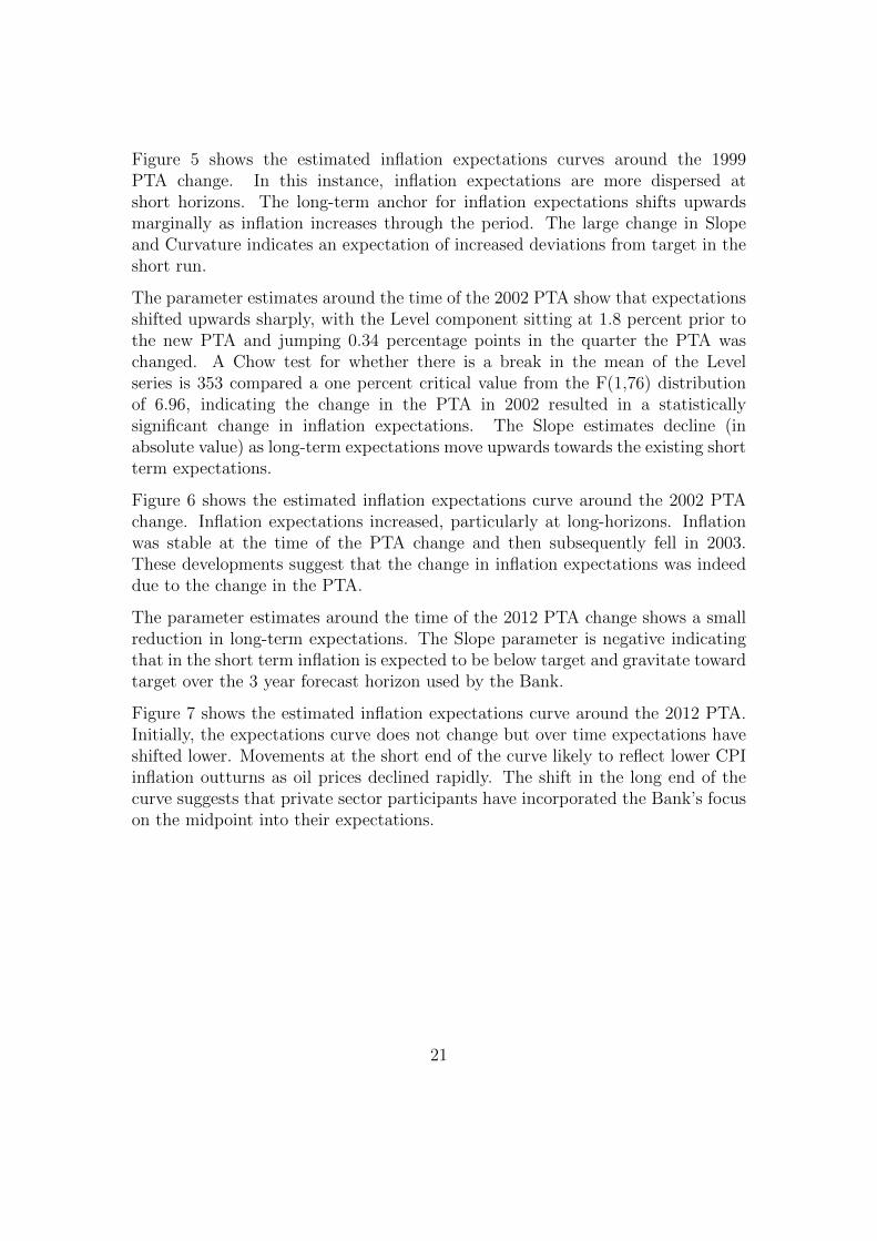
Figure 5 shows the estimated inflation expectations curves around the 1999PTA change. In this instance, inflation expectations are more dispersed atshort horizons. The long-term anchor for inflation expectations shifts upwardsmarginally as inflation increases through the period. The large change in Slopeand Curvature indicates an expectation of increased deviations from target in theshort run.

The parameter estimates around the time of the 2002 PTA show that expectationsshifted upwards sharply, with the Level component sitting at 1.8 percent prior tothe new PTA and jumping 0.34 percentage points in the quarter the PTA waschanged. A Chow test for whether there is a break in the mean of the Levelseries is 353 compared a one percent critical value from the F(1,76) distributionof 6.96, indicating the change in the PTA in 2002 resulted in a statisticallysignificant change in inflation expectations. The Slope estimates decline (inabsolute value) as long-term expectations move upwards towards the existing shortterm expectations.

Figure 6 shows the estimated inflation expectations curve around the 2002 PTAchange. Inflation expectations increased, particularly at long-horizons. Inflationwas stable at the time of the PTA change and then subsequently fell in 2003.These developments suggest that the change in inflation expectations was indeeddue to the change in the PTA.

The parameter estimates around the time of the 2012 PTA change shows a smallreduction in long-term expectations. The Slope parameter is negative indicatingthat in the short term inflation is expected to be below target and gravitate towardtarget over the 3 year forecast horizon used by the Bank.

Figure 7 shows the estimated inflation expectations curve around the 2012 PTA.Initially, the expectations curve does not change but over time expectations haveshifted lower. Movements at the short end of the curve likely to reflect lower CPIinflation outturns as oil prices declined rapidly. The shift in the long end of thecurve suggests that private sector participants have incorporated the Bank’s focuson the midpoint into their expectations.

21

Inflation expectation curves following PTA changes

Figure 4: 1996 PTA

Horizon (years)0 2 4 6 8 10

Per

cent

1

2

3

4

1996Q31996Q4 (quarter of new PTA)1997Q11997Q4

1996:3 1997:1 1997:31

2

3 CPI inflation

Figure 5: 1999 PTA

Horizon (years)0 2 4 6 8 10

Per

cent

1

2

3

4

1999Q31999Q4 (quarter of new PTA)2000Q12000Q4

1999:3 2000:1 2000:3

1

2

3

4CPI inflation

Figure 6: 2002 PTA

Horizon (years)0 2 4 6 8 10

Per

cent

1

2

3

4

2002Q22002Q3 (quarter of new PTA)2002Q42003Q3

2002:32003:12003:31

2

3CPI inflation

Figure 7: 2012 PTA

Horizon (years)0 2 4 6 8 10

Per

cent

1

2

3

42012Q22012Q3 (quarter of new PTA)2012Q42013Q32016Q1

2012:1 2014:1 2016:1

1

2 CPI inflation

Note: The expectation curves in figures 4 to 7 show inflation expectations behaved one quarter

before the PTA change, the quarter of the change, one quarter following, and one year after.

The insert graph shows headline CPI inflation at the time.

22

4.2 Testing the Impact of PTA Changes on InflationExpectations

The results above suggest that changes to the inflation target do affect inflationexpectations. However, examining only periods around PTA changes may bemisleading. Changes in expectations may occur because of changes in pastinflation.

To test whether changes in the PTA influences long-run inflation expectations, weregress the Level from the inflation expectations curve on a constant, the laggedLevel, distributed lags of inflation, and dummy variables indicating the timing ofthe changes to the PTA. Lags of annual inflation are included in the regressionto control for the impact of past inflation on inflation expectations. The laggedLevel term is included to account for the persistence typically observed in inflationexpectations. Thus we estimate the following regression

β̂1t = α0 + α1β̂1t−1 +2∑

k=0

γkπt−k∗4 +4∑

k=1

δkDk + εt (8)

where β̂1t is the estimate of the Level from equation 7 at time t, πt is annualinflation at time t, and D1 = 1 if t ≥1994Q4 and 0 otherwise, D2 = 1 if t ≥2002Q3 and 0 otherwise, otherwise, D3 = 1 if t ≥ 2012Q3 and 0 otherwise, and εtis a regression residual. The parameter values γk show the marginal impact of anew PTA relative to the preceding period.

The results of this regression are reported in Table 3. First, lagged annualinflation and the lagged Level are statistically significant at the 5 and 10 percentlevel, respectively. Thus controlling for past inflation and inflation expectations isnecessary. This evidence indicates that inflation expectations do adjust adaptivelyto past inflation.

The estimated coefficient on the dummy variable for the 2002 PTA changeis positive and statistically significant, indicating that inflation expectationsimmediately increased 0.19 percentage points when the target midpoint wasincreased 0.5 percentage points. The coefficient estimates on the 1999 and2012 dummies are not statistically significant but economically the changes areconsistent with the changes to the PTA. Following the introduction of thesecondary objectives but no change to the numerical inflation target in the 1999PTA, inflation expectations increased 0.05 percentage points. This is consistentwith more flexibility in achieving the inflation target. The 2012 PTA change, whichput more emphasis on the 2 percent midpoint of the target range, is associated

23

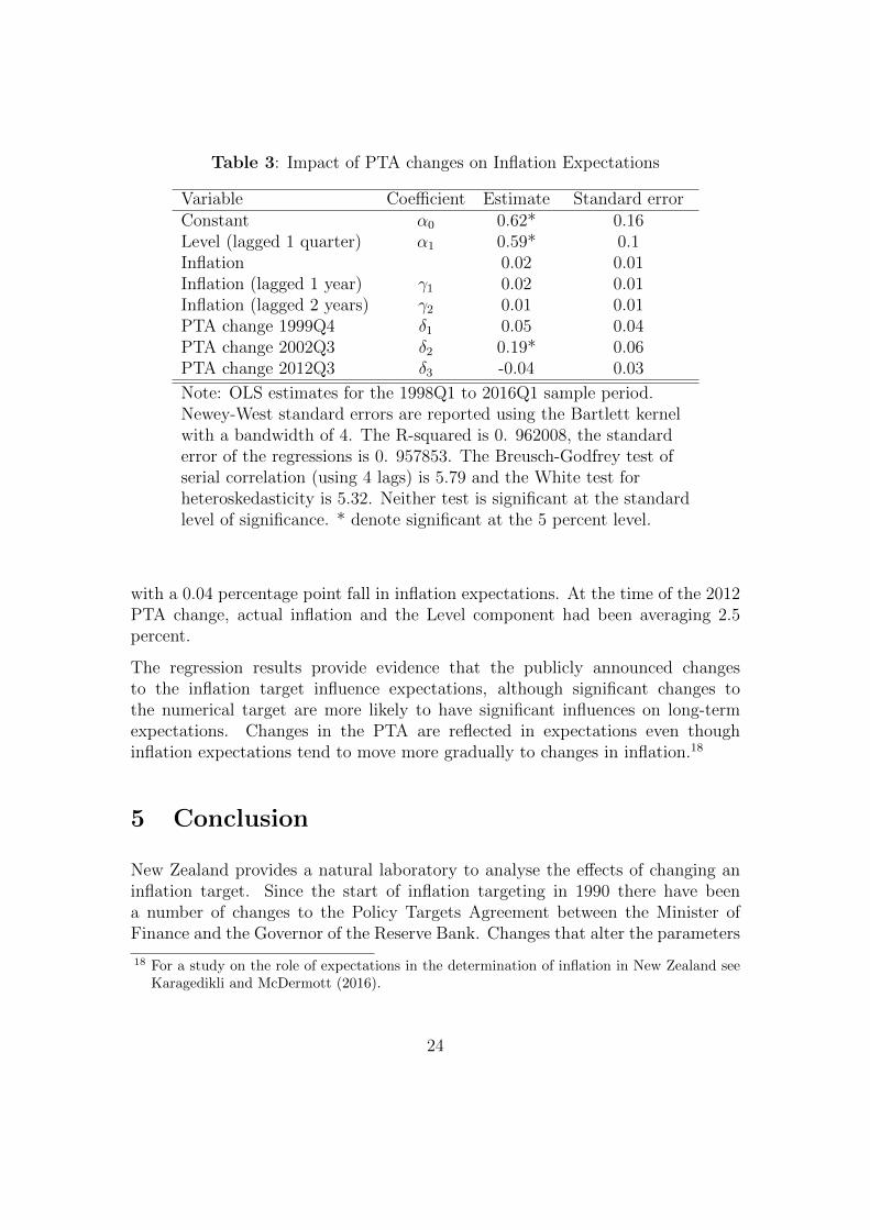
Table 3: Impact of PTA changes on Inflation Expectations

Variable Coefficient Estimate Standard errorConstant α0 0.62* 0.16Level (lagged 1 quarter) α1 0.59* 0.1Inflation 0.02 0.01Inflation (lagged 1 year) γ1 0.02 0.01Inflation (lagged 2 years) γ2 0.01 0.01PTA change 1999Q4 δ1 0.05 0.04PTA change 2002Q3 δ2 0.19* 0.06PTA change 2012Q3 δ3 -0.04 0.03

Note: OLS estimates for the 1998Q1 to 2016Q1 sample period.Newey-West standard errors are reported using the Bartlett kernelwith a bandwidth of 4. The R-squared is 0. 962008, the standarderror of the regressions is 0. 957853. The Breusch-Godfrey test ofserial correlation (using 4 lags) is 5.79 and the White test forheteroskedasticity is 5.32. Neither test is significant at the standardlevel of significance. * denote significant at the 5 percent level.

with a 0.04 percentage point fall in inflation expectations. At the time of the 2012PTA change, actual inflation and the Level component had been averaging 2.5percent.

The regression results provide evidence that the publicly announced changesto the inflation target influence expectations, although significant changes tothe numerical target are more likely to have significant influences on long-termexpectations. Changes in the PTA are reflected in expectations even thoughinflation expectations tend to move more gradually to changes in inflation.18

5 Conclusion

New Zealand provides a natural laboratory to analyse the effects of changing aninflation target. Since the start of inflation targeting in 1990 there have beena number of changes to the Policy Targets Agreement between the Minister ofFinance and the Governor of the Reserve Bank. Changes that alter the parameters

18 For a study on the role of expectations in the determination of inflation in New Zealand seeKaragedikli and McDermott (2016).

24

of the inflation target have tended to occur on average every five years or so (theterm of a Governor’s appointment).

The process of inflation expectations formation is pivotal for predicting the effectsof a change to the inflation target. The Reserve Bank’s DSGE model of the NewZealand economy, NZSIM, predicts that a change in the inflation target will resultin a permanent one-for-one change in inflation and inflation expectations. Themodel also predicts that changes in the target may result in a temporary boost tooutput under adaptive expectations but there is no boost to output under rationalexpectations.

Evidence suggests that there is some degree of inertia in inflation expectations.That being the case, the probability of being at the Zero Lower Bound (ZLB)in New Zealand for five consecutive quarters is likely low, given the current 2percent target midpoint. Any increase in the target would seem to offer diminishingprotection from the ZLB but a reduction in the target would likely increase therisk of the ZLB, on average over the business cycle.

Evidence from estimated inflation expectation curves show that changes in theinflation target are quickly reflected in inflation expectations. Particularly strikingis the estimated immediate 0.19 percentage point increase in inflation expectationswhen the target midpoint was increased 0.5 percentage points in 2002. Thus wecan conclude that changing the numerical inflation target is likely to feed intoinflation expectations but unlikely to provide even a temporary boost to outputor other real economic variables.

The periodic ’fine-tuning’ of the inflation target has steadily introduced moreflexibility into the New Zealand regime. This flexibility has been gained whilestill keeping inflation expectations anchored.

25

Appendices

NZSIM Model Equations

Here we list the NZSIM model equations used to generate the macroeconomicresponses of an inflation target change and the probability of hitting the zero lowerbound. The version of the model listed here is, with exception of the monetarypolicy rule, the model used for the production of forecasts in the Reserve Bank ofNew Zealand’s Monetary Policy Statement.

1. Consumption

ct =1

1 + χ(Etct+1 + χct−1)

−α1Et∆yt+1 − α2 [irt − πet + ζbt + εct ] + ωc (pH,t − pt)

where εct is the consumption shock, ct is consumption, yt is GDP, irt the nominalretail interest rate, bt is foreign debt, pH,t, is the house price level, pt is πt is inflationand the e subscript above any variable means adaptive expectations for the nextquarter. The notation Et preceding a variable means rational expectations takenat time t. In this equation and subsequent equations the variables of interest arelog-deviations from steady state so, for example, yt can equivalently by denotedas the output gap.

2. Non-tradable inflation Phillips curve

πN,t − γNπN,t−1 = β(πeN,t − γNπN,t

)+ κN [wt − pN,t + ϕyt] + εNt

where εNt is the non-tradable inflation shock, πN,t is non-tradable inflation, wt isthe nominal wage, and pN,t is the non-tradable price level,

3. Tradable inflation Phillips curve

πT,t − γTπT,t−1 = β(πeT,t − γTπT,t

)+κT

[τT (p∗M,t − st − pT,t) + (1− τT )(pN,t − pT,t)

]+ εTt

where εTt is the tradable inflation shock, πT,t is tradable inflation, st is the nominalexchange rate, pT,t is the tradable price level and pM,t is the import price. The ∗

superscript refers to the foreign variable equivalent.

4. Wage Phillips Curve

πw,t − γwπw,t−1 = β(πew,t − γwπw,t

)+ κw

[ ηαyt − (wt − pt)

]+ εwt

where εwt is the nominal wage shock and πw,t is nominal wage inflation.

26

5. Policy interest rate rule

it = φiit−1 + (1− φi) {π̄t + φπ (Etπt+1 − π̄t + φyyt})}+ εit

where εit the monetary policy shock, it is the nominal policy interest rate and π̄tis the inflation target.19

6. Retail interest rateirt = it + εirt

where εirt is the retail interest rate shock.

7. Uncovered interest parity

it − i∗t + ∆Etst+1 + εst = τ[it−1 − i∗t−1 + ∆st

]where εst is the exchange rate shock.

8. GDP expenditure

yt =C

Yct +

IKYikt +

IHYiht +

G

Ygt +

X

Yxt −

M

Ymt

where ikt is capital investment, iht is housing investment, gt is governmentspending, xt is exports, mt is imports. Capital letters without time subscriptsrefer to steady state values.

19 The monetary policy rule specified here is different to the one used in NZSIM. First, wehave included a time variant inflation target so we can generate impuse response functionsfrom a change to the target. Second, we have simplified the rule so interest rates react toexpected inflation 1 quarter ahead rather than 4 quarters ahead. We avoid using the 4 quarterahead rule because under full rational expectations it is possible to generate policy responseswith plausible parameters in the interest rate reaction function that result in indeterminateequilibria. Introducing some inertia in the policy rule eliminates the indeterminacy andproduces simulations that are qualitatively similar to those reported here. However, using a 1quarter ahead policy rule simplifies the experiments and makes the results easier to interpret.

27

9. Import demand

mt =CTYT

(ct − ξ(pT,t − pt) + εmt )

+IkTYT

(ikt − ξi (1− υT,Ik) (pT,t − pN,t))

+IhTYT

(iht − ξ (1− υT,Ih) (pT,t − pN,t))

+GT

YT(gt − ξ (1− υT,g) (pT,t − pN,t))

+XT

YT(xt − ξ (1− υT,x) (pT,t − pN,t))

+

(1− M

YT

)ξT (pT,t − pM,t)

where εmt is the import demand shock, YT , CT , Ik,T , Ih,T , GT , and XT are thesteady state values of the tradables parts of aggregate demand components.

10. Tradable share of consumption

CTYT

= υTcy

yty

11. Tradable share of capital investment

IkTYT

= υT,Ikiki

yty

12. Tradable share of housing investment

IhTYT

= υT,Ihihi

yty

13. Tradable share of government spending

GT

YT= υT,g

gy

yty

14. Tradable share of exportsXT

YT= υT,x

xy

yty

28

15. Tradable share of output

yty = vT ∗ cy + vT.Ik ∗ iki+ vT,Ih ∗ ihi+ vT,g ∗ gy + vT,x ∗ xy

vT = 0.4359, vT,Ik = 1, vT,Ih = 0.2, vT,g = 0.6, vT,x = 0.4

16. Shares

cy = 0.5852, gy = 0.1936, iy = 0.2063, xy = 0.3069,

my = 0.2920, ihi = 0.05434, iki = 0.1520

17. Balance of payments

bt −1

βbt−1 =

PMM

Y(pM,t +mt)−

PXX

Y(pX,t + xt) + εbt

where εbt , is the debt shock, pX,t is the export price and any capital letters withouttime subscripts refer to steady state values.

18. Adaptive Expectations

πeN,t+1 = ρ1πeN,t + (1− ρ1)[ρ2EtπN,t+1 + (1− ρ2)πN,t−1] + εet

πeT,t+1 = ρ1πT,t + (1− ρ1)[ρ2EtπT,t+1 + (1− ρ2)πT,t−1] + εet

πew,t+1 = ρ1πew,t + (1− ρ1)[ρ2Etπw,t+1 + (1− ρ2)πw,t−1]

πet = 0.55πeN,t + 0.45πeT,t

where εet is the inflation expectations shock.

19. House price inflation

πH,t − δH,1πH,t−1 = δH,2πeH,t − δH,3 (irt − πet + ζbt) + δH,4imt

−δH,5(pH,t − pt)− δH,6bt + επHt

where επHt is the house price inflation shock, πH,t is house price inflation and imt

is migration.

20. Housing investment

iH,t = ΥH,1πH,t + ΥH,2imt −ΥH,3 (it − πet + ζbt) + εHt

where εHt is the housing investment shock.

29

21. Capital investmentiK,t = γiyt + εKt

where εKt is the capital investment shock.

22. Export determination

xt = ρxxxt−1 + µ(pX,t − ρt) + y∗t + εXt

where εXt is the export shock.

23. Government expenditure process

gt = ρggt−1 + εGt

where εGt is the government expenditure shock.

24. Migration processimt = ρimimt−1 + εimt

where εimt is the migration shock.

25. Foreign sector

i∗t = ρif i∗t−1 + εift

y∗t = ρyfy∗t−1 + εyft

p∗t = p∗t−1 + π∗t

p∗t = ρpfp∗t−1 + εpft

p∗X,t = ρXp∗X,t−1 + εpXt

p∗M,t = ρMp∗M,t−1 + εpMt

where εift is the foreign interest rate shock, εyft is the foreign output shock, εift isthe foreign interest rate shock, εpft is the foreign price level shock, εpXt is the exportprice shock, and εpMt is the import price shock.

30

References

Aruoba, S. B. (2014), “Term Structure of Inflation Expectations and RealInterest Rates: The Effect of Unconventional Monetary Policy,” University ofMaryland and Federal Reserve Bank of Minneapolis.

Aruoba, S. B (2016), “Term structures of inflation expectations and real interestrates. Working Papers 16-9, “Federal Reserve Bank of Philadelphia.

Blanchard, O., G. Dell’Ariccia, and P. Mauro (2010), “RethinkingMacroeconomic Policy, “IMF Staff Position Note SPN/10/03.

Bollard, A. (2002), “The Evolution of Monetary Policy in New Zealand,” speechdelivered on 25 November 2002.

Bollard, A. (2008), “Flexibility and the Limits of Inflation Targeting,” speechdelivered on 30 July 2008.

Bollard, A. and O. Karagedikli (2006), “Inflation Targeting in the NewZealand Experience and Some Lessons,” paper prepared for the Inflation TargetingPerformance and Challenges Conference by the Central Bank of the Republic ofTurkey, Istanbul, 19-20 January, 2006.

Buiter, W. (2010), “Don’t Raise the Inflation Target, Remove the Zero LowerBound on Nominal Interest Rates Instead,” Global Macro View Citigroup GlobalMarkets (March 5).

Burgess, S, Fernandez-Corugedo, E, Groth, C, Harrison, R, Monti, F,Theodoridis, K and Waldron, M (2013), “The Bank of England’s forecastingplatform: COMPASS, MAPS, EASE and the suite of models” , Bank of EnglandWorking Paper No. 471.

Calomiris, C. W. and S. H. Haber (2014), Fragile by Design: ThePolitical Origins of Banking Crisis and Scarce Credit, Princeton University Press,Princeton.

Diebold, F. X. and G. D. Rudebusch, (2012), Yield Curve Modeling andForecasting: The Dynamic Nelson-Siegel Approach, Economics Books, PrincetonUniversity Press, 1(1), number 9895.

Doan, T., R. B. Litterman, and C. A. Sims (1983), “Forecasting andConditional Projection Using Realistic Prior Distributions,” National Bureau ofEconomic Research, 1202.

Dorich J, Johnston M K, Mendes R R, Murchison S, Zhang Y. (2013),“ToTEM II: An Updated Version of the Bank of Canada’s Quarterly Projection

31

Model,” Technical report, Bank of Canada 2013.

Granville, B. (2013), Remembering Inflation, Princeton University Press,Princeton.

Gurkaynak, R., and Wright, J. (2012), “Macroeconomics and the termstructure,” Journal of Economic Literature, 50, 331-67

Hall, V. B. and C. J. McDermott (2009), “The New Zealand business cycle,”Econometric Theory, 25, 1050-1069.

Hall, V. B. and C. J. McDermott (2011), “A Quarterly Post-Second WorldWar Real GDP Series for New Zealand,” New Zealand Economic Papers, 45(3),273-298.

Hall, V. B. and C. J. McDermott (2015), “Recessions and Recoveries inNew Zealand’s Post-Second World War Business Cycles,” SEF Working paper:09/2015.

Hargreaves, D. (2002), “The Implications of Modified InflationTargets for the Behaviour of Inflation,” in Reserve Bank of NewZealand, The Policy Targets Agreement: Reserve Bank Briefing Noteand Related Papers, September, 57-59, http://www.rbnz.govt.nz/monetary policy/policy targets agreement/0124760.html

Hargreaves, D, H Kite, and B Hodgetts (2006), “Modelling New Zealandinflation in a Phillips curve,” Reserve Bank of New Zealand Bulletin, Vol 69 (3),23-37.

Hunt, C. (2004), “Interpreting clause 4(b) of the Policy Targets Agreement:Avoiding Unnecessary Instability in Output, Interest Rates and the ExchangeRate,” Reserve Bank of New Zealand Bulletin, 67, No. 2, 5-20.

Jacob P and Munro A (2016), “A macroprudential stable funding requirementand monetary policy in a small open economy,” Reserve Bank of New ZealandDiscussion Paper DP 2016/04.

Justiniano, A. and B. Preston (2010), “Monetary Policy and Uncertaintyin an Empirical Small Open-Economy Model, ” Journal of Applied Econometrics,25(1), 93-128.

Kam, T., K. Lees, and P. Liu (2009), “Uncovering the Hit List for SmallInflation Targeters: A Bayesian Structural Analysis, ” Journal of Money, Creditand Banking, 41(4), 583-618.

Kamber, G., C. McDonald, N. Sander, and K. Theodoridis (2015), “A

32

Structural Forecasting Model for New Zealand: NZSIM,” Reserve Bank of NewZealand.

Karagedikli, O., and C. J. McDermott (2016), “Inflation expectations andthe decline of inflation in New Zealand ” Reserve Bank of New Zealand.

Khan, M. S. and A. S. Senhadji (2001), “Threshold Effects in theRelationship Between Inflation and Growth,” IMF Staff Papers, 48(1), 1-21.

Kendall, R. and T. Ng (2013), “The 2012 Policy Targets Agreement: AnEvolution in Flexible Inflation Targeting in New Zealand,” Reserve Bank of NewZealand Bulletin 76(4), 3-12.

Lewis, M. (2015), “Forecasting with Macro-Finance Models: Applications toUnited States and New Zealand,” Master of Commerce in Economics Thesis,Victoria University of Wellington, School of Economics and Finance.

Lewis M (2016), “Inflation expectations curve: a tool for monitoring inflationexpectations.” Reserve Bank of New Zealand Analytical Note, AN2016/01.

Orphanides, A. and J. C. Williams (2005), “Imperfect Knowledge, InflationExpectations, and Monetary Policy,” in B. S. Bernanke and M. Woodford (eds.)The Inflation-Targeting Debate, National Bureau of Economic Research, Chicago.

Razzak, W. (1997), “Testing the rationality of the National Bank of NewZealand’s survey data,” Reserve Bank of New Zealand Discussion Paper, G97/5.

Reifschneider, D. and J. C. Williams (2000), “Three Lessons for MonetaryPolicy in a Low Inflation Era,” Journal of Money, Credit and Banking, 32, 936-966.

Reserve Bank of New Zealand (2000), “The Evolution of the Policy TargetsAgreements,” http://www.rbnz.govt.nz/monetary_policy/about_monetary_

policy/0096846.html

Reserve Bank of New Zealand (2007), “Supporting PaperA1: Monetary Policy Framework and Goals,” in ReserveBank of New Zealand: Select Committee Submission, 24-35,http://www.rbnz.govt.nz/monetary policy/about monetary policy/3075587.pdf

Richardson A. and R. Williams (2015), “Estimating New Zealand’s NeutralInterest Rate,” Reserve Bank of New Zealand Analytical Note, AN2015/05.

Reinhart, C. M. and K. S. Rogoff (2009), This Time is Different: EightCenturies of Financial Folly, Princeton University Press, Princeton.

Stock, J. S, and Watson, W. W (2002), “Macroeconomic forecasting usingdiffusion indexes. ” Journal of Business and Economic Statistics, 20(2), 147-162.

33

Waggoner, D. F. and T. Zha (1999), “Conditional Forecasts in DynamicMultivariate Models,” Review of Economics and Statistics, 81(4), 639-651.

Wright, J. H (2009), “Forecasting US inflation by Basyesian model averaging,”Journal of Forecasting, 28(2), 131-144.

34