draft - optimization · pdf filedraft multi-period portfolio optimization with alpha decay...

DRAFT

Axioma Research Paper

No.

February 19, 2015

Multi-period portfolio optimization with alpha

decay

The traditional Markowitz MVO approach is based on a single-period model. Single period models do not utilize any data ordecisions beyond the rebalancing time horizon with the result thattheir policies are myopic in nature. For long-term investors, multi-period optimization offers the opportunity to make wait-and-seepolicy decisions by including approximate forecasts and long-termpolicy decisions beyond the rebalancing time horizon. We considerportfolio optimization with a composite alpha signal that is com-posed of a short-term and a long-term alpha signal. The short-termalpha better predicts returns at the end of the rebalancing periodbut it decays quickly, i.e., it has less memory of its previous values.On the other hand, the long-term alpha has less predictive powerthan the short-term alpha but it decays slowly. We develop a simpletwo stage multi-period model that incorporates this alpha model toconstruct the optimal portfolio at the end of the rebalancing pe-riod. We compare this model with the traditional single-periodMVO model on a simulated example from Israelov & Katz [12] andalso a large strategy with realistic constraints and show that themulti-period model tends to generate portfolios that are likely tohave a better realized performance.

DRAFT

Multi-period portfolio optimization with alpha decay

Multi-period portfolio optimization with alphadecay

Kartik Sivaramakrishnan, Vishv Jeet, and Dieter Vandenbussche

1 Introduction

The traditional Markowitz MVO approach is based on a single-period setting that limits itsapplicability to long-term investors with liabilities and goals at different times in the future.Single-period optimization does not use any data and decisions beyond the rebalancing timehorizon with the result that its policies are myopic in nature. More importantly, single-period optimization does not account for the fact that a decision made in a rebalancingtoday affects decisions made in future rebalancings. This is a drawback even if the rebal-ancing is done periodically in light of new information. A multi-period model has severalstages with the first stage representing the current rebalancing and stages two and beyondrepresenting future rebalancings. The model allows the simultaneous rebalancing of a singleportfolio across different periods (extending beyond the rebalancing time horizon) in a singleoptimization problem. Each stage in the model has its own data forecasts, objectives, andpolicy decisions and the stages in successive periods are coupled together. In most cases,we are only interested in the first-stage solution since the solution to the remaining stagescan be updated as new information becomes available. The first-stage solution to the multi-period model incorporates a wait-and-see feature, since it is aware of future decisions anddata forecasts through the other stages in the model.

One issue with multi-period models is that they require forecast information beyond therebalancing time horizon that is subject to greater uncertainty. A second issue is that theresulting model is complex and requires greater solution time. Despite these issues, multi-period models have generated a lot of interest in the financial community since they attemptto model the future dynamics of the portfolio taking into account data and decisions beyondthe rebalancing time horizon. This leads to better solutions implemented today than wouldbe possible with a myopic single-period model.

Multi-period models have found several applications in finance. The following list is byno means exhaustive.

1. Trade scheduling: This is a common problem that is handled by large sell-side firmsand investment banks. A trade scheduling problem aims to get from an initial portfolioto a target portfolio in stages while trading off the risk and market-impact across allthese stages. The risk term in the objective forces the trading to happen quickly (move

Axioma 2

DRAFT


slowly and the market will move you!). The market-impact term in the objective slowsdown the trading to avoid the market prices moving in an unfavorable fashion (movequickly and you will move the market!). One must consider implementation shortfall,which is defined as the difference between the prevailing portfolio price and the effectiveexecution price for the proposed trade schedule. In a seminal paper, Almgren & Chriss[1] minimize the first two moments of implementation shortfall in a Markowitz mean-variance framework to determine the optimal trade schedule. They show that the firstmoment of the implementation shortfall models the market-impact and the secondmoment of implementation shortfall models risk. A similar model is also consideredin Grinold & Kahn [10]. Multi-period models that only trade-off market-impact andtime varying alpha are considered in Bertsimas & Lo [4]. The market-impact is usuallya non-linear power function (quadratic, three-halves, five-thirds) of the transactions(see Almgren et al. [2] for more details). Almgren & Chriss consider a quadraticmarket-impact model and do not include realistic constraints (such as long-only) forthe different stages in their multi-period model. Consequently, their model resemblesthe classical LQR problem from optimal control and they are able to derive a closed-form solution for their model by solving an algebraic Riccati equation.

2. Transition management and dynamic benchmark tracking: This is a passivemanagement framework where the aim is to track a benchmark or target portfolioclosely over time while minimizing the tracking error and market-impact across severalstages. Some of the stages can also include potential cash flows and portfolio injections.This is a common problem faced by large ETF providers who receive cash inflows andportfolios from investors over time and need to track a dynamic index closely. Blakeet al. [5] provide a good overview of multi-period optimization models in this area.

3. Tax-optimization: Taxes are special transaction cost models that penalize sales.Moreover, short-term gains are taxed at a substantially larger rate than long-termgains. Multi-period models can be used to delay the sale of assets in the portfolio inorder to take advantage of the long-term rates. The multi-period tax optimization isespecially challenging since the tax liability is a function of both the current share priceas well as the prevailing price when the asset was purchased. Multi-period portfoliotaxes models are considered in DeMiguel & Uppal [6] and more recently in Haugh etal. [11].

4. Alpha-decay: This is the application that we consider in this paper. In a typi-cal portfolio application, the composite alpha signal is a composition of signals withdifferent strengths and decay rates. Usually, the signals that carry more informa-tion decay quickly. In an influential paper, Garleanu & Pedersen [7] consider an un-constrained infinite-dimensional multi-period model that trades off risk, return, andquadratic market-impact. This model provides an opportunity to trade-off the strengthof the fast decaying signals and the persistence (memory) of the slow decaying signals.Garleanu & Pedersen construct an optimal policy for their model using dynamic pro-gramming. We discuss their model in some detail in Section 3.

Axioma 3

DRAFT


We consider a simple variant of the alpha-decay use case in this paper. The investor hasan alpha that is composed of two signals: (a) a short-term signal that better predicts thereturns at the end of the rebalancing time horizon but decays quickly, i.e., the signal in thenext rebalancing period is very different to the one in the current period, and (b) a long-termsignal that has more memory, i.e., the signal in the next rebalancing period is similar to theone in the current period but is poorer at predicting the realized returns at the end of therebalancing period than the short-term signal. A short-term investor who only chases theshort-term signal would incur high turnover as he rebalances his portfolio over time. This willeat into his returns. The long-term investor who only chases the long-term signal is giving upthe valuable alpha in the short-term signal. So the dilemma faced by the investor is this: Howdo I trade-off the strength of the short-term signal and the slow-decay of the long-term signalwhile satisfying all my other mandates? We consider a simple two-stage multi-period modelthat is embedded in a rolling-horizon backtester to address this question. The backtestersolves a two-stage multi-period model in each period and returns the first-stage portfolio asthe final holdings. These holdings are then rolled-forward using the actual realized returnsand a new two-stage multi-period model is solved in the next period and so on. To avoidany confusion, we will use periods to represent the different time periods (iterations) in thebacktest and stages to represent the different rebalancings in a point-in-time multi-periodmodel. Our model is inspired by the work in Garleanu & Pedersen [7] but we also considerrealistic portfolio constraints in each stage of the model. We must emphasize that one needsan optimizer to solve a multi-period model with realistic constraints. The model no longeradmits a closed form solution and also specialized approaches such as dynamic programmingno longer apply.

There has been a lot of other work in the alpha-decay case. Israelov and Katz [12] developan interesting informed trading heuristic that uses uses the short-term alpha signal to timethe portfolio’s trades; specifically, they continue with a trade only if both short-term andthe long-term components of the composite alpha signal agree on the direction of the tradeand otherwise cancel it. They test their heuristic on a realistic example and a simulatedexample with promising results. Grinold [8, 9], Qian et al. [13], and Sneddon [14] each solvea static auxiliary problem that trades-off signal strength and time decay to determine thesignal weights. These weights are then used in a single-period model to generate the portfolioholdings.

This paper is organized as follows: Section 2 introduces multi-period portfolio models.Section 3 gives a brief overview of the Garleanu-Pedersen model that is the inspiration forour work. Section 4 presents our rolling-horizon two-stage multi-period algorithm for thetwo alpha problem. Section 5 compares the performance of our multi-period algorithmwith a single-period backtester on a simulated example that is taken from Israelov & Katz[12]. Section 6 presents our computational experiences with the multi-period algorithm ona large strategy with realistic constraints. Section 7 presents our conclusions. The technicalappendix gives the mathematical details of some of our main results.

Axioma 4

DRAFT


2 Multi-period models

Consider the following two-stage multi-period model

max (α1)Tw1 − δTC(∆w1)− γ(w1)TΣw1 + E [α2]Tw2 − δTC(∆w2)− γ(w2)TΣw2

s.t. w2 = (1 + r)w1 + ∆w2,w1 = w0 + ∆w1,w1 ∈ C1,w2 ∈ C2

(1)

that trades off risk, return, and transaction costs across two stages. The variables w1 andw2 represent the final holdings of the portfolio and ∆w1 and ∆w2 represent the trades madein the first and second stages of the model, respectively. The initial holdings w0 are known.The first set of equations describe the final holdings of the portfolio in the second stage asthe rolled-forward holdings from the first stage plus the trades made in the second stage.Note that these equations actually couple stages one and two. The third and the fourthset of equations represent the constraints that the portfolio must satisfy in the first andsecond stages of the model. We will hereafter refer to these set of constraints as independentconstraints since they only involve the holding and the trade variables of a stage.

The inputs to the multi-period model include:

1. w0 - the initial portfolio holdings vector.

2. α1 - the alpha vector for the first stage.

3. E [α2] - the expected alpha vector for the second stage. The expected alpha dependson the choice of our alpha uncertainty model and we present some details when weconsider our two alpha model in Section 4.

4. TC(∆w1) and TC(∆w2) that represent the transaction cost (TC) models for the firstand second stages, respectively. Each TC model is associated with a coefficient δ inthe objective function.

5. The risk model Σ and the risk aversion coefficient γ. For simplicity, we will assumethat both stages use the same risk model and risk aversion coefficient.

6. The estimate r for the roll-forward returns. The portfolios generated by the multi-period optimization are sensitive to this choice!

7. The independent constraints in the first and second stages.

The first stage of the multi-period model represents the current rebalancing that the investoris interested in. The length of this stage corresponds to the rebalancing time horizon thatthe investor would consider in a single-period setting. The investor knows that she willbe rebalancing their portfolio in the future and the second stage of the multi-period modelrepresents this future rebalancing with its own data estimates and decisions. Note that the

Axioma 5

DRAFT


decisions made in the second stage are a function of the decisions made in the first stage andthe data for the second stage. The objective terms in the second stage of the multi-periodmodel are usually discounted in practice as they represent rebalancings that are farther outin time. Note that w2 really represents the expected second stage portfolio holdings sincethe alpha for this stage is not known precisely. We are especially interested in the first-stageholdings w1 since the holdings from the second stage can be updated as more informationbecomes available. We want to know how the data and the decisions in the second stage ofthe model help us make informed decisions in the first stage. Finally, we must emphasizethat it is hard to come with good roll-forward estimates for the multi-period model and wewill assume that r = 0 throughout this paper.

3 The Garleanu-Pedersen model

We briefly describe the Garleanu-Pedersen multi-period portfolio model [7] that incorporatesalpha-decay in this section. Consider a composite alpha signal over n assets that is composedof k factors with varying decay rates. The composite alpha in stage j of the multi-periodmodel is given by

αj = Bf j (2)

where the factors evolve as

f j = (I − φ)f j−1 + εj (3)

where Φ is a diagonal matrix of factor decay-rates and εj is a random variable with zero meanand finite variance. Garleanu and Pedersen consider the following unconstrained infinitedimensional multi-period portfolio problem to determine the trades (w1, w2, . . . , )

maxw1,w2,...

E1

(∑t

−δ2

(∆wt

)TΣ(∆wt

)+(

(αt)Twt − γ

2

(wt)T

Σ(wt)))

(4)

that trades off the present value of all the future excess expected return (alpha), risk, re-turn, and transaction costs. 1 The expectation is taken over the random αt. The risk isrepresented by the variance of the portfolio returns, where Σ is the asset covariance matrix.The transaction costs are modeled by a quadratic function with the costs proportional torisk. This assumption enables us to derive a simple closed form solution for the model. Thepositive scalars γ, δ represent the risk and TC aversion parameters, respectively. Using thelaw of total expectation, we can write the objective function in (4) as

Eα1

(OBJ1 +

(Eα2|α1

(OBJ2 +

(Eα3|α1,α2

(OBJ3 + . . .+

)))))(5)

where

OBJj = −δ2

(∆wj

)TΣ(∆wj

)+ (αj)Twj − γ

2

(wj)T

Σ(wj)

1We are neglecting the discount term in the Garleanu-Pedersen model to simplify the exposition.

Axioma 6

DRAFT


is the objective function in stage j. The outer expectation Eα1 in (5) is the expectation overthe random α1, the inner expectation Eα2|α1 is the conditional expectation of α2 with α1

known, and Eα3|α1,α2 is the conditional expectation of α3 with α1 and α2 both known andso on.

The Markowitz portfolio at stage j that only trades off risk and return during this periodis given by

MVj = (γΣ)−1Bf j (6)

Consider an investor who performs the following single-period optimization

maxwj

(αj)Twj − γ2

(wj)T

Σ (wj)− δ2

(∆wj)T

Σ (∆wj) (7)

in stage j with initial holdings wj−1 where ∆wj = (wj − wj−1). The optimal single-periodportfolio for this investor is given by

wjspo =δ

γ + δwj−1 +

γ

γ + δMVj. (8)

Garleanu & Pedersen [7] use dynamic programming to derive an expression for the portfolioholdings in the different stages. They show that the optimal portfolio at stage j is

wj =(

1− a

δ

)wj−1 +

a

δTARj (9)

where

a =

√γ2 + 4γδ − γ

2(10)

is a positive scalar and

TARj = (γΣ)−1B

f j,1(1 +

φ1a

γ

)...

f j,k(1 +

φka

γ

)

(11)

is the target portfolio that trades off risk and return. Comparing (8) and (9), we see that theoptimal multi-period portfolio uses the target portfolio instead of the Markowitz portfolio atstage j. Moreover, the target portfolio is basically the Markowitz portfolio with each factorscaled down by its decay rate.

Axioma 7

DRAFT


4 Two alpha multi-period model

We apply the two-stage multi-period model that we introduced in Section 2 to the two alphacase in this section. The composite alpha signal in the model is constructed from (a) a strongand rapidly decaying short-term signal, and (b) a weak and persistent long-term signal.

We embed this multi-period model in a rolling-horizon backtester. Our model resem-bles the model predictive approach (see Chapter 6 in Bertsekas [3]) to solving stochasticmulti-stage problems where one (a) solves a sequence of deterministic two-stage multi-periodmodels conditional on the available information, (b) implements only the first-stage solu-tion, (c) refines the second-stage solution with new information as it becomes available.One can show that the multi-stage rolling-horizon backtester generates the same trades asthe dynamic programming approach of Garleanu-Pedersen for the unconstrained case withquadratic transaction costs and the same number of stages. On the other hand, the rolling-backtester can incorporate realistic constraints and different transaction cost models (linear,piecewise-linear, three-halves) in the multi-period model, where closed-form solutions are notavailable and dynamic programming is no longer a viable approach. We must also emphasizethat our rolling-horizon model is a heuristic approach to solving the stochastic multi-stagemodel with realistic constraints. It is however known to generate good solutions in practice(see Bertsekas [3]).

The alpha signal in stage j of the multi-period model at time t is given by

αt,j = λjsαts + λjlα

tl (12)

where αts, αtl are the short-term and long-term alpha signals and λjs, λ

jl are their associated

weights. Furthermore the signal follow a first-order autoregressive process given by

αjs = σsαj−1s + εjs,

αjl = σlαj−1l + εjl ,

(13)

where σs, σl ∈ (0, 1) denote the short-term and long-term autocorrelations and εts and εtldenote random short-term and long-term innovations with zero mean and finite variance.Note that (13) resembles the Garleanu-Pedersen alpha-decay model, where we assume thatthe uncertainty is baked into the signals themselves. The autocorrelations measure how closetoday’s signal is to yesterday’s signal while the innovations represent the new informationflowing into the signals in each period. We have λs > λl since the short-term signal betterpredicts the immediate returns, i.e., the returns at the end of the previous period. On theother hand, we have σs < σl since the long-term signal has more memory. From (13), wecan compute the conditional expected alpha in the next period given the current alpha as

E [αjs|αj−1s ] = σsαj−1s ,

E[αjl |α

j−1l

]= σlα

j−1l .

(14)

We are now ready to present our multi-period backtester.

Multi-period backtester

Axioma 8

DRAFT


1. Start the algorithm with a set of initial holdings w0. Estimate the short-term andlong-term alpha weights λs, λl, the risk and TC aversion parameters γ, δ, and the riskmodel Σ. We will assume a quadratic TC model that is proportional to the risk andthat the alpha weights, risk and TC aversion parameters, and risk model are fixed overtime.

2. For period t, estimate the short-term alpha αts and the long-term alpha αtl .

3. Solve the following two-stage multi-period model

maxw1,w2

2∑j=1

E[αt,j]Twj − γ

2

(wj)T

Σ(wj)− δ

2

(wj − wj−1

)TΣ(wj − wj−1

)(15)

where w0 is known and

E [αt,1] = λsαts + λlα

tl ,

E [αt,2] = σsλsαts + σlλlα

tl

(16)

at the beginning of period t. We use (14) to derive the expression of the expectedsecond stage alpha in the multi-period model. We hold the first-stage holding w1

throughout period t.

4. Calculate the net return in period t as the realized portfolio return minus transactioncosts.

5. Set t = t+1, the initial holding for the next period to be w1 rolled-forward, and returnto Step 2.

A few comments are now in order:

1. We only implement the first-stage decision of the two period model. We are notinterested in the second-stage decision as it can be refined as more information becomesavailable in the future. As we show below, the second-stage in the multi-period modelinduces a wait-and-see feature in the first-stage decision.

2. We show in the Technical Appendix that the first stage solution for (15) is

w1 = ψδw0︸︷︷︸Initial portfolio

+ ψΣ−1((

1 +δσsδ + γ

)λsα

ts

)︸︷︷︸

ST Signal strength component

+ ψΣ−1((

1 +δσlδ + γ

)λlα

tl

)︸︷︷︸

LT Time-decay component

(17)

Axioma 9

DRAFT


where

ψ =γ + δ

(γ + δ)2 + δγ.

This shows that the first stage solution is a non-negative combination of three portfo-lios:

(a) Initial portfolio - to reduce transaction costs.

(b) Signal strength component - this component is the sum of the Markowitz portfoliosfor the short-term signal (trading-off risk and short-term return) over the twostages. It emphasizes the better predictive power of the short-term signal.

(c) Time-decay component - this component is the sum of the Markowitz portfoliosfor the long-term signal (trading-off risk and long-term return) over the two stages.It emphasizes the slow decay of the long-term signal.

3. We compare our multi-period backtester with a single-period backtester. The single-period backtester follows all the steps of the rolling multi-period algorithm exceptthat it uses different weights on the short-term and long-term signals, a different TCaversion parameter, and solves the following single-period model

maxw

(λ̄sα

ts + λ̄lα

tl

)Tw − γ

2wTΣw − δ̄

2

(w − w0

)TΣ(w − w0

)(18)

in Step 3 of the algorithm. One can easily show that the solution to this model inperiod t is

wspo =δ̄

δ̄ + γw0 + Σ−1

(λ̄sα

ts + λ̄lα

tl

). (19)

4. Comparing (17) and (18), we show in the Technical Appendix that one can recoverthe first-stage solution of the multi-period algorithm in a single-period backtestingframework if we choose the single-period TC aversion and short-term and long-termweights as

δ̄ =

(γ + δ

γ + 2δ

)δ,

λ̄s = ψ(γ + δ̄

)(1 +

σsδ

δ + γ

)λs,

λ̄l = ψ(γ + δ̄

)(1 +

σlδ

δ + γ

)λl.

(20)

For these choice of parameters the single-period backtester is equivalent to the multi-period algorithm. As we show in the Technical Appendix, the single-period backtesterhas to increase the weight on the long-term signal in order to recover the multi-periodsolution.

Axioma 10

DRAFT


The interesting question is what happens to the first stage solution when one adds infinitelymany stages to the model in (15). When the number of stages is very large, we can use theGarleanu-Pedersen result to show that the first stage solution at time t converges to

w1 =(

1− a

δ

)w0 +

a

δΣ−1

(λs

γ + a (1− σs)αts +

λlγ + a (1− σl)

αtl

)(21)

where

a =

√γ2 + 4γρ− γ

2.

Comparing this expression with (18), one can show that the single-period backtester isequivalent to the multi-period algorithm with infinitely many stages by choosing

δ̄ =γ

a

(1− a

δ

)δ,

λ̄s =aλs

δ (γ + a (1− σs)),

λ̄l =aλl

δ (γ + a (1− σl)).

(22)

Given that one can replicate the multi-period setting in a single-period framework, whyshould one be interested in a multi-period portfolio model? The answer is that the equiv-alence between the multi-period and single-period setups holds only under limited settings.Some settings may require changing more single-period data parameters and there are severalcases where the equivalence breaks down.

1. Consider a two period model where one maximizes the two-term alpha subject toconstraints that impose upper bounds on risk and TC in the two stages. In this case,one can use the duality theory of convex optimization (see the Technical Appendix fordetails) to rewrite this problem as (15) where γ and δ are the optimal duals to the riskand TC constraints. These duals will vary over time and so an equivalent single-periodframework would have to dynamically change the TC aversion and more importantlythe short-term and long-term signal weights over time.

2. If the strategy contains realistic long-only constraints or combinatorial constraints suchas cardinality and threshold constraints, then it is impossible to find a set of single-period parameters for which the single-period backtester is equivalent to the rollingmulti-period algorithm.

We would like to reiterate that multi-period optimization allows the investor to naturallytrade-off signal strength and decay in one consolidated optimization problem. The signalweights in the first stage of the model can be chosen entirely on signal strength. Theseweights are appropriately down-weighted in the later stages of the model based on the signaldecay; the short-term signal weight in each of these stages gets downweighted more than thecorresponding long-term signal weight.

Axioma 11

DRAFT


5 Single period vs Multiperiod: Simulated results

This section describes the simulation that we used to compare the multi-period and single-period algorithms. We use the methodology from the simulated example in the Israelov-Katzpaper [12] to generate the short-term and the long-term alphas. Both backtests are run overT = 10, 000 periods with a portfolio universe of 10 assets. We briefly describe the alphageneration process and refer the reader to [12] for more details.

1. The realized returns are simulated from a normal distribution with zero mean, 20percent annualized volatility, and 0.5 correlation between the assets.

2. The short-term and long-term alphas are generated from two independent exponen-tially weighted moving averages (EWMA) (with appropriate half-lives) of the realizedreturns plus noise. The EWMA construction proceeds backwards in time so that thealphas can explain future returns. The short-term and long-term alphas describe afirst-order autoregressive AR(1) process

αts =2

3αt−1s + εts,

αtl =260

261αt−1l + εtl ,

(23)

with autocorrelations σs = 23

and σl = 260261

, respectively.

3. The short-term and long-term alphas are then converted into z-scores (cross-sectionallyacross the 10 assets).

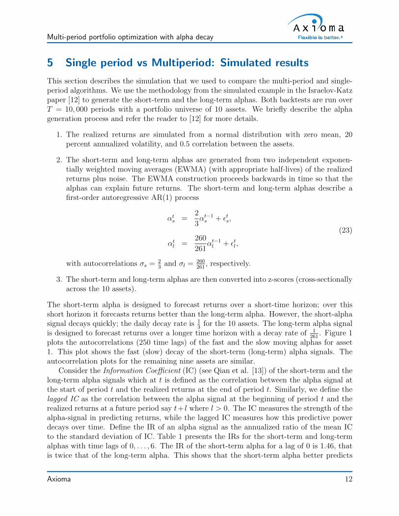
The short-term alpha is designed to forecast returns over a short-time horizon; over thisshort horizon it forecasts returns better than the long-term alpha. However, the short-alphasignal decays quickly; the daily decay rate is 1

3for the 10 assets. The long-term alpha signal

is designed to forecast returns over a longer time horizon with a decay rate of 1261

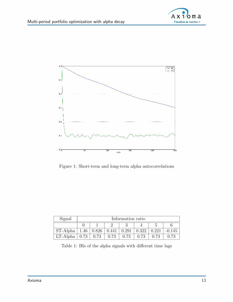
. Figure 1plots the autocorrelations (250 time lags) of the fast and the slow moving alphas for asset1. This plot shows the fast (slow) decay of the short-term (long-term) alpha signals. Theautocorrelation plots for the remaining nine assets are similar.

Consider the Information Coefficient (IC) (see Qian et al. [13]) of the short-term and thelong-term alpha signals which at t is defined as the correlation between the alpha signal atthe start of period t and the realized returns at the end of period t. Similarly, we define thelagged IC as the correlation between the alpha signal at the beginning of period t and therealized returns at a future period say t+ l where l > 0. The IC measures the strength of thealpha-signal in predicting returns, while the lagged IC measures how this predictive powerdecays over time. Define the IR of an alpha signal as the annualized ratio of the mean ICto the standard deviation of IC. Table 1 presents the IRs for the short-term and long-termalphas with time lags of 0, . . . , 6. The IR of the short-term alpha for a lag of 0 is 1.46, thatis twice that of the long-term alpha. This shows that the short-term alpha better predicts

Axioma 12

DRAFT


Figure 1: Short-term and long-term alpha autocorrelations

Signal Information ratio

0 1 2 3 4 5 6ST-Alpha 1.46 0.826 0.441 0.291 0.322 0.221 -0.145LT-Alpha 0.73 0.73 0.73 0.73 0.73 0.73 0.73

Table 1: IRs of the alpha signals with different time lags

Axioma 13

DRAFT


immediate returns. On the other hand, the predictive power of the short-term alpha fallsquickly as we increase the number of lags. With a lag of more than 7 periods, the predictivepower of the short-term alpha drops to zero. The long-term alpha, however, retains most ofits predictive ability as one increases the number of lags.

We now describe the multi-period and the single-period backtest setups on this two-alphamodel. The multi-period backtester solves a two stage model in each period.

1. Generate 100 different time series of returns and alphas using the EWMA constructionin equation (23) with different seeds.

2. For each seed, we run the multi-period and single-period backtests with 10 assetscovering 10000 periods where one solves the following model in each period.

• Maximize two-term alpha with the long-term weights varying from 10 − 100%.For the multi-period model, the short-term and long-term alphas in the secondstage are down-weighted by their autocorrelations as described in equation (15).

• Dollar-neutral and risk bound of 10%. These constraints are applied to bothstages of the multi-period model.

• We run two cases:

– Case 1 has a 32

market-impact term in the objective, this market-impact termis applied to both stages of the multi-period model

– Case 2 has a round-trip turnover constraint that is applied to both stages ofthe multi-period model. Moreover, in Case 2, we also fix the leverage of thedollar-neutral portfolio to the reference size, i.e., the long and the short sidesof the portfolio sum up to the reference size of the portfolio.

• Fix the weight on the market-impact term in Case 1 and the round-trip turnoverbound in Case 2.

Note that we run a frontier using the single-period and multi-period approaches by varyingthe relative weights on the short-term and the long-term signals. The upper exhibit of Figure2 presents a scatter plot of the maximum Sharpe ratios obtained using the two approacheswith the MI objective (Case 1) for the 100 seeds. Note that for each seed, the maximumSharpe ratio is the best Sharpe ratio obtained over the signal weight frontier, where we varythe weight on the long-term signal from 10 − 100%. We have also included the 45 degreeline as a reference in this exhibit. All dots above the 45 degree line represent scenarioswhere the multi-period setup returned better maximum Sharpe ratios than the single-periodsetup. By comparing the best Sharpe ratio of both approaches across the frontier, we wantto see whether we can recover the multi-period solution in a single-period setting. We seethat most of the dots are clustered across the 45 degree line indicating that both frontierbacktests produce similar maximum Sharpe ratios. This is not surprising given that themodel in Case 1 is very close to the unconstrained models that we considered in Section4. There we made the case that it is possible to recover the multi-period solution in a

Axioma 14

DRAFT


(a) Max Sharpe ratios

(b) Average Sharpe ratios

Figure 2: SPO vs MPO: Case 1 - Market Impact Objective

Axioma 15

DRAFT


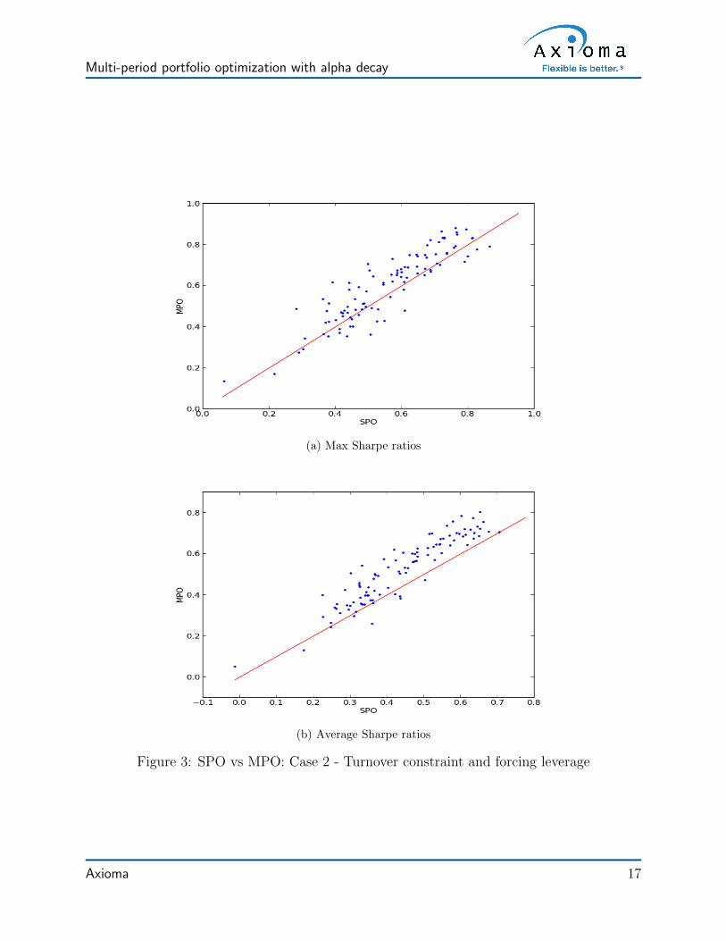
single-period framework by appropriately changing some of the parameters in the single-period model - notably the weight on the short-term and the long-term signals. Looselyspeaking we can interpret the result in the upper exhibit of Figure 2 as follows: In a simplestrategy, if a portfolio manager is good at picking the alpha weights, then they can recoverthe performance of multi-period backtest in a single-period setting. The lower exhibit ofFigure 2 presents a scatter plot of the average Sharpe ratios obtained using the single-periodand multi-period frontier backtests with the MI objective (Case 1) for the 100 seeds. Thisplot tells a different story; most of the dots are above and some are well above the 45 degreereference line indicating that the multi-period backtester is able to deliver better Sharperatios on average. Loosely speaking we can interpret these results as follows: If a portfoliomanager is average at picking the alpha weights, then the multi-period setting with its in-built alpha-decay feature is more likely to deliver a better realized performance. The upperexhibit of Figure 3 presents a scatter plot of the maximum Sharpe ratios obtained using thesingle-period and multi-period frontier backtests with the turnover constraint and enforcingleverage (Case 2) for the 100 seeds. About 70% of the dots are above the 45 degree lineindicating the multi-period backtester has a better realized performance when more realisticand complicated combinatorial constraints are present in the model. In this case, it is moredifficult to achieve the multi-period performance in a single-period setting by just varyingthe weights on the alpha signals. The lower exhibit of Figure 3 presents a scatter plot ofthe average Sharpe ratios obtained using the two approaches for Case 2 over the 100 seeds.Almost all the dots are above the 45 degree line. Moreover, a greater proportion of thesedots are above the 45 degree line than in the lower exhibit of Figure 2 indicating that onaverage the multi-period backtester is more likely to deliver a better Sharpe ratio with amore complicated strategy.

6 Single period vs Multiperiod: Realistic backtests

This section describes the realistic backtest that we used to compare the multi-period andsingle-period algorithms. The short-term and the long-term alphas are obtained from twoindependent exponentially weighted moving averages (with a half-life of 0.3 months for theshort-term signal and 6 months for the long-term signal) of the 24 month forward-lookingS&P 500 realized returns plus noise. They are then standardized to z-scores. We generate 30different series of the short-term and long-term signals by varying the noise. Table 2 presents

Signal Information ratio

0 1 2 3ST-Alpha 1.81 0.30 -0.06 0.11LT-Alpha 1.24 1.15 0.94 0.82

Table 2: IRs of the alpha signals with different time lags

the IRs of the alpha signals with different time lags (each lag corresponds to a month).

Axioma 16

DRAFT



(b) Average Sharpe ratios

Figure 3: SPO vs MPO: Case 2 - Turnover constraint and forcing leverage

Axioma 17

DRAFT


The short-term signal better predicts the immediate returns than the long-term signal butits predictive power decays rapidly as we increase the number of lags. In particular, theshort-term alpha loses its predictive power within two months. The autocorrelations for theshort-term and long-term signals are 0.1 and 0.9, respectively.

We now run the following backtest with the single-period and multi-period algorithms:

1. Monthly backtest run from January 1997 to January 2012.

2. Maximize two-term alpha with the long-term weights varying from 10− 100%.

3. Our investment universe includes all the assets in the S&P 500.

4. Portfolio is long-only and fully-invested.

5. Tracking error of 3% with respect to the S&P 500.

6. Turnover limit of 10%.

7. Limit absolute asset trades to 5% of the asset’s 20-day ADV.

8. Use 10 bps for buys/sells when computing the net realized returns in each period.

Our multi-period backtester has the following features:

1. It solves a two stage multi-period model in each rebalancing.

2. The short-term and long-term alphas are down-weighted by their autocorrelations inthe second period. More specifically, the short-term signal weight in the second periodis 0.1 times its weight in the first period. The long-term signal weight in the secondperiod is 0.9 times its weight in the first period.

3. The multi-period model has a copy of the realistic constraints in both stages.

4. We continue to assume that the roll-forward return estimates are zero.

The upper exhibit of Figure 4 presents a scatter plot of the maximum single-period andmulti-period Sharpe ratios for the 30 seeds. About 53% of the dots lie above the 45 degreereference line showing that the multi-period backtester performs slightly better than thesingle-period backtester over these 30 seeds. The lower exhibit of Figure 4 presents a scatterplot of the mean Sharpe ratios for the 30 seeds. About 96% of the dots are now above the 45degree line. This shows that the multi-period backtester performs better much better thanthe single-period backtester when the portfolio manager is ”average” at picking the signalweights.

Axioma 18

DRAFT



(b) Mean Sharpe ratios

Figure 4: SPO vs MPO: Realistic setup

Axioma 19

DRAFT


7 Conclusions

We consider a portfolio construction model with a composite alpha signal that is composedof a short-term and a long-term alpha signal. This is a classical problem in investing andalpha signals that can be classified as short-term or long-term are already part of the arsenalof most quantitative researchers. We develop a simple two-stage multi-period model thatincorporates such an alpha model and generates a more informed first-stage decision with theavailable information. The first-stage decision also incorporates a wait-and-see feature sincethis decision is aware of data and decisions beyond the rebalancing time horizon throughthe second stage in the multi-period model. We embed the two-stage multi-period model ina rolling-horizon backtester and compare this algorithm with the traditional single-periodbacktester on a simulated example from Israelov & Katz [12] and also a sizable, more realisticstrategy. We show that the multi-period algorithm generates portfolios with a better realizedperformance in both sets of experiments.

It is clear that the multi-period algorithm implicitly favors the long-term signal in theoptimization and one can attempt to reproduce this in the single-period backtester by as-signing more weight to the long-term signal. This is why we generated frontiers for thesingle-period and multi-period approaches by varying the relative weights on the short-termand the long-term signals. By comparing the best (over the frontier) Sharpe ratio of eachapproach, one can see how close one can get to the multi-period portfolio performance byusing the single-period approach. We observe that with the more complex, more constrainedstrategies, even the best Sharpe ratio with the single-period model is generally not thatclose to the best Sharpe ratio obtained via the multi-period model. This indicates that onecannot recover the multi-period portfolios by choosing a fixed adjustment (through time)to the signal weights in the single-period approach. One can still hope for a time varyingadjustment of the single-period signal weights that would allow a single-period model achievethe benefits of the multi-period approach. However, the complexity of finding such weightadjustments in realistic strategies makes this impractical.

We also used a scaled version of the short-term alpha as an estimate for the roll-forwardreturns. We found that the performance of the multi-period approach was (a) similar to thezero roll-forward estimate case that we reported in the paper, and (b) was not very sensitiveto the choice of these roll-forward returns. We also performed an additional experiment,where we use the true forward looking returns in the roll-forward estimate, but we did NOTuse those true returns in the alpha estimates. In this case, we found that the performance ofthe multi-period approach drastically improved. Obviously, this is not of practical use butwe do think that coming up with good roll-forward estimates that improve the performanceof the multi-period algorithm is a worthy topic for future investigation.

To summarize, multi-period optimization allows the investor to naturally trade-off signalstrength and decay in one consolidated optimization problem. The signal weights in the firststage of the model can be chosen entirely on signal strength. These weights are appropriatelydown-weighted in the later stages of the model based on the signal decay; the short-termsignal weight in each of these stages gets down-weighted more than the corresponding long-term signal weight. An optimizer is necessary to solve the multi-period model with realistic

Axioma 20

DRAFT


constraints and our computational experience indicates that the solution time taken by therolling-horizon two stage multi-period algorithm is comparable to a single-period backtesterin practice.

References

[1] R. Almgren and N. Chriss, Optimal execution of portfolio transactions, Journal ofRisk (Winter 2000/2001), pp. 5-39.

[2] R. Almgren, C. Thum, E. Hauptmann, and H. Li, Direct estimation of equitymarket impact, Risk, 18(2005), pp. 57-62.

[3] D. Bertsekas, Dynamic Programming and Optimal Control, Volume I, Athena Scien-tific, Nashua, NH 03061-0805, 2012.

[4] D. Bertsimas and A. Lo, Optimal control of execution costs, Journal of FinancialMarkets, 1(1998), pp. 1-50.

[5] C. Blake, D. Peitrich, and A. Ulitsky, The right tool for the job: Using Multi-period optimization in transitions, Trading, Summer 2003, pp. 33-37.

[6] V. DeMiguel and R. Uppal, Portfolio investment with the exact tax basis via non-linear programming, Management Science, 51(2005), pp. 277-290.

[7] N. Garleanu and L.H. Pedersen, Dynamic trading with predictable returns andtransaction costs, Journal of Finance, 68(6), December 2013, pp 2309-2339.

[8] R. Grinold, Dynamic portfolio analysis, The Journal of Portfolio Management, Fall2007, pp. 12-26.

[9] R. Grinold, Signal weighting, The Journal of Portfolio Management, Summer 2010,pp. 1-11.

[10] R.C. Grinold and R.N. Kahn, Active Portfolio Management, 2nd edition, McGraw-Hill, New York, NY, 2000.

[11] M. Haugh, G. Iyengar, and C. Wang, Tax-aware dynamic asset allocation, Tech-nical Report, Department of IE and OR, Columbia University, March 2014. Available athttp://papers.ssrn.com/sol3/papers.cfm?abstract id=2374966

[12] R. Israelov and M. Katz, To Trade or Not to Trade? Informed trading with Short-Term signals for Long-Term investors, Financial Analysts Journal, 67(5), 2011, pp. 23-36.

[13] E. Qian, E.H. Sorensen, and R. Hua, Information horizon, portfolio turnover,and optimal alpha models, The Journal of Portfolio Management, 34(Fall 2007), 2007,pp. 27-40.

Axioma 21

DRAFT


[14] L. Sneddon, The tortoise and the hare: Portfolio dynamics for active managers, TheJournal of Investing, Winter 2008, pp. 106-111.

Axioma 22

DRAFT


Technical Appendix: Recovering the first-stage MPO solu-tion in an SPO framework

We compare simple unconstrained two-stage multi-period (MPO) and single-period (SPO)models that trade off risk, return, and transaction costs. The alpha signal for the two modelsare constructed from short-term and long-term alpha signals.

We assume that the alpha signal for the two models has two components:

1. A strong but fast decaying alpha signal αs.

2. A weak but slowly decaying alpha signal αl.

To obtain analytic solutions, we consider a quadratic transaction cost model

TC(∆w) =1

2(∆w)T Λ∆w, (24)

with Λ = δΣ, where Σ is the covariance matrix that defines risk. These assumptions greatlysimplify the expressions for the optimal SPO and MPO portfolios in the following discussions.

Consider the following two-stage MPO model

maxw1,w2

(α1)Tw1 + E

[α2]Tw2 −

2∑k=1

(γ

2

(wk)T

Σwk − δ

2

(∆wk

)TΣ∆wk

)(25)

with ∆w2 = w2−w1 and ∆w1 = w1−w0 where w0 is known. The alphas for the two stagesare given by

α1 = λsαs + λlαl,E [α2] = σsλsαs + σlλlαl

(26)

where λs, λl represent the weights of the short-term and long-term signals and σs, σl representthe short-term and long-term autocorrelations. We will assume that

1. λs > λl since the short-term signal better explains the realized returns at the end ofthe rebalancing period.

2. σs < σl since the long-term signal decays more slowly.

The optimality conditions for (25) are

E [α2]− γΣw2 − δΣ∆w2 = 0,

α1 − γΣw1 − δΣ∆w1 + δΣ∆w2 = 0.(27)

The first equation in (27) gives

w2 =δ

γ + δw1 +

1

γ + δΣ−1E

[α2]. (28)

Axioma 23

DRAFT


Substituting this expression for w2 in the second equation in (27) in turn and simplifying,we have

w1 = aΣ−1α1 + aδw0 + aδ

δ + γΣ−1E

[α2]

(29)

where

a =γ + δ

(γ + δ)2 + δγ, (30)

and

MV1 =1

γΣ−1α1,

=1

γΣ−1 (λlαl + λsαs) ,

E[MV2

]=

1

γΣ−1E

[α2],

=1

γΣ−1 (σlλlαl + σsλsαs)

(31)

are the first and second stage Markowitz portfolios.This shows that the optimal first-stage MPO portfolio is a non-negative combination of

three portfolios:

1. Initial portfolio (to reduce transaction costs).

2. Markowitz portfolio from the first stage that heavily weights the short-term alpha sincethis alpha has better predictive power (signal strength component).

3. The expected Markowitz portfolio from the second stage that overweights the long-termalpha since this component decays more slowly (alpha-decay component).

We are interested in constructing the first-stage multi-period solution in a SPO model byonly changing:

1. The weight δ > 0 on the transaction cost term.

2. The weights λs > 0 on the short-term signal and λl > 0 on the long-term signal in thecomposite alpha.

Consider the SPO model

maxw

((α)T w − γ

2(w)T Σw

)− δ̄

2(∆w)T Σ∆w (32)

Axioma 24

DRAFT


where ∆w = w − w0 with w0 known and the alpha signal is given by

α = λ̄sαs + λ̄lαl. (33)

Note that the SPO model uses the same risk model and risk aversion parameter as the MPOmodel. It can be easily shown that the optimal solution is given by

wSPO =γ

δ̄ + γMV1 +

δ̄

δ̄ + γw0 (34)

where

MV1 =1

γΣ−1α1,

=1

γΣ−1

(λ̄sα

1s + λ̄lα

1l

) (35)

is the unconstrained Markowitz portfolio that only trades off risk and return.This shows that the SPO optimal portfolio is a convex combination of two portfolios:

1. Initial portfolio (to reduce transaction costs).

2. Markowitz portfolio that heavily weights the short-term alpha since this alpha hasbetter predictive power.

We want to choose δ̄, λ̄s, and λ̄l so that we recover the optimal first-stage MPO portfolio(29) in the SPO solution (34).

Equating (29) and (34) and simplifying, we have

δ̄ =(γ + δ)δ

(γ + 2δ),

λ̄s = a(γ + δ̄

)(1 +

σsδ

δ + γ

)λs,

λ̄l = a(γ + δ̄

)(1 +

σlδ

δ + γ

)λl,

(36)

where the scalar a is given in (10). These are the values of the SPO parameters that helpone recover the first-stage optimal MPO solution in the SPO setting.

Note that

λ̄sλ̄l

=

1 +σsδ

δ + γ

1 +σlδ

δ + γ

λsλl

<λsλl

Axioma 25

DRAFT


since σl > σs. This indicates that the SPO model has to increase the weight on the long-termsignal in order to capture its slow time decay.

Now consider the following MPO model

maxw1,w2

(α1)Tw1 + E

[α2]Tw2 −

2∑k=1

γ

2

(wk)TQwk

s.t.1

2

(∆w1

)TΣ(∆w1

)≤ κ,

1

2

(∆w2

)TΣ(∆w2

)≤ κ

(37)

where the transaction costs are modeled as constraints.Using the duality theory of convex optimization, this problem can be equivalently written

as

maxw1,w2

(α1)Tw1 + E

[α2]Tw2 −

2∑k=1

γ

2

(wk)TQwk − δ∗1

2

(∆w1

)TΣ(∆w1

)− δ∗2

2

(∆w2

)TΣ(∆w2

)where δ∗1 and δ∗2 are the optimal dual variables for the two TC constraints. We can alsouse the procedure described earlier to determine the SPO parameters needed to recover theoptimal first-stage MPO portfolio. Note that the procedure needs to be reworked a bit sinceδ∗1 and δ∗2 are different.

Moreover, if one were to embed the SPO and the MPO models in a backtest, thenone would need to modify the TC aversion and the weights on the short-term and long-term signals in the SPO model during each period of the backtest in order to consistentlyreproduce the optimal first-stage MPO portfolio.

Axioma 26

US and Canada: 212-991-4500

Europe: +44 20 7856 2451

Asia: +852-8203-2790

New York Office

Axioma, Inc.

17 State Street

Suite 2550

New York, NY 10004

Phone: 212-991-4500

Fax: 212-991-4539

Atlanta Office

Axioma, Inc.

8800 Roswell Road

Building B, Suite 295

Atlanta, GA 30350

Phone: 678-672-5400

Fax: 678-672-5401

London Office

Axioma, (UK) Ltd.

30 Crown Place London, EC2A 4EB

Phone: +44 (0) 20 7856 2451

Fax: +44 (0) 20 3006 8747

Hong Kong Office

Axioma, (HK) Ltd.

Unit B, 17/F, Entertainment Building

30 Queen’s Road Central

Hong Kong

Phone: +852-8203-2790

Fax: +852-8203-2774

San Francisco Office

Axioma, Inc.

201 Mission Street

Suite #2230

San Francisco, CA 94105

Phone: 415-614-4170

Fax: 415-614-4169

Singapore Office

Axioma, (Asia) Pte Ltd.

30 Raffles Place

#23-00 Chevron House

Singapore 048622

Phone: +65 6233 6835

Fax: +65 6233 6891

Geneva Office

Axioma CH

Rue du Rhone 69, 2nd Floor

1207 Geneva, Switzerland

Phone: +33 611 96 81 53

Sales: [email protected]

Client Support: [email protected]

Careers: [email protected]

DRAFT

draft - optimization · pdf filedraft multi-period portfolio optimization with alpha decay...

Documents