Drift-Free Humanoid State Estimationfusing Kinematic, Inertial and LIDAR sensing

Maurice F. Fallon1, Matthew Antone, Nicholas Roy and Seth Teller2

Abstract— This paper describes an algorithm for the prob-abilistic fusion of sensor data from a variety of modalities(inertial, kinematic and LIDAR) to produce a single consistentposition estimate for a walking humanoid. Of specific interest isour approach for continuous LIDAR-based localization whichmaintains reliable drift-free alignment to a prior map usinga Gaussian Particle Filter. This module can be bootstrappedby constructing the map on-the-fly and performs robustly ina variety of challenging field situations. We also discuss atwo-tier estimation hierarchy which preserves registration tothis map and other objects in the robot’s vicinity while alsocontributing to direct low-level control of a Boston DynamicsAtlas robot. Extensive experimental demonstrations illustratehow the approach can enable the humanoid to walk over uneventerrain without stopping (for tens of minutes), which wouldotherwise not be possible. We characterize the performanceof the estimator for each sensor modality and discuss thecomputational requirements.

I. INTRODUCTION

Dynamic locomotion of legged robotic systems remainsan open and challenging research problem whose solutionwill enable humanoids to perform tasks in and reach placesinaccessible to wheeled or tracked robots. Several researchinstitutions are developing walking and running robots with arange of form factors, from all-terrain quadrupeds operatingoutdoors to experimental bipedal runners which have yet toleave the laboratory.

Locomotion is a typical closed-loop control problemwhose primary input consists of the state of the robot —namely, the 6-DOF pose and velocity of its pelvis, as wellas the configuration of its joints. Accurate, timely estimatesof the robot state not only facilitate effective control fordynamic whole-body motions such as walking, but alsoenable a greater degree of task autonomy via consistentknowledge of the surrounding environment and the locationsof objects within it.

A. Related Work

One common class of estimation method is based ondynamics (e.g., [1]), and relies on knowledge of the con-troller outputs and a motion model of the humanoid toinfer the state of the robot’s centers of mass and pressure.Errors in link center-of-mass modeling and the presence ofunpredictable forces (e.g., from the robot’s support/powertether or external contacts) are accounted for by appendingan additional process model for each class of disturbance.

2The authors are with the Computer Science and Artificial IntelligenceLaboratory, Massachusetts Institute of Technology, USA. Maurice F. Fallonis also with the Department of Informatics, University of Edinburgh, UK.mfallon,antone,nickroy,teller@csail.mit.edu

Fig. 1. The Atlas robot contains 28 hydraulically actuated joints, and itsprimary sensing is provided by the Carnegie Robotics Multisense SL sensorhead which is equipped with a rotating LIDAR scanner and a stereo camera.(photo credits: Boston Dynamics and CRL)

In [2], the authors extend this approach and apply it tothe Atlas robot (which we are also using in our work).They discuss the computational challenges of formulatinga single extended Kalman filter (EKF) for a humanoid withmany degrees of freedom, and propose instead to estimatethe pelvis position and joint dynamics in separate filters.

An EKF-based estimator is presented in [3] for aquadruped that uses a sensor-based prediction model andcreates filter corrections using foothold measurements. Thisapproach incorporates the positions of footholds into thestate vector (using a point model for each foot) and givesparticular consideration to consistency and observabilityanalysis. Recently this approach was extended to bipedallocomotion [4] with results presented on a simulated SAR-COS robot. The primary contribution was extension of thealgorithm to a biped with a full foot plate, which requires a6 DOF constraint on the foot frame.

Finally, there has also been work in coupling odometryestimates to a higher-level navigation system. Localizationof a quadruped (in 3 DOF) against a prior terrain map wasexplored by [5] using a particle filter.

All of the above works utilize only proprioceptive sensing.While visual mapping is an active area of research — forinstance [6] demonstrated loop-closing and visual keyframeregistration to known landmarks in a laboratory setting —it has not been widely adopted for field operations. Highcomputational cost, latency, and sensitivity to environmentalconditions (e.g., illumination and visual texture content)all present substantial challenges for robust vision-basedmapping onboard a humanoid. Hornung et al. [7] utilized aLIDAR sensor to localize an Aldebaran NAO robot within a

multi-level environment, thus circumventing many problemsinherent to visual sensing; our work also adopts LIDAR asthe primary exteroceptive sensor for localization.

B. Overview

This paper presents a state estimation algorithm that com-bines measurements from three distinct sensing modalities— inertial, leg kinematics, and LIDAR — into a singleconsistent estimate of the robot’s pelvis link via probabilisticfusion. The estimator does not require elaborate dynamicsmodels; like [4], we couple foot placements and leg kine-matics with inertial predictions in an EKF framework, andlike [2], we consider pelvis pose separately from joint states.Our primary novel contributions are (1) incorporation ofexteroceptive sensing to achieve reliable drift-free alignmentto a prior map while walking using a Gaussian ParticleFilter (GPF) to apply position corrections derived from eachLIDAR scan; and (2) extensive experimental validation ofthe algorithm on a real humanoid robot.

The estimator is demonstrated using the Boston Dynamics(BDI) Atlas humanoid (Figure 1) provided to our researchteam for the ongoing DARPA Robotics Challenge (DRC).The LIDAR-based localization component was specificallymotivated by the slow locomotion rates achieved in theDRC Trials in December 2013: due to position drift onthe order of 2 cm per footstep, teams typically took justtwo steps at a time to traverse uneven terrain, pausingperiodically to manually re-localize the robot and to createnew motion plans with respect to the environment. As wepush toward enabling greater autonomy in task execution —e.g., walking for several minutes at a time with manipulationactions interspersed — a continuous localization capabilitybecomes critically important, as it allows the robot to retainaccurate and consistent reference to terrain maps and objectsof interest in its vicinity.

In Section II we present an overview of our requirementsfor state estimation and discuss two different use cases forour approach. Then in Sections III–V we discuss how eachsensor stream can be abstracted to a basic probabilisticmeasurement suitable for fusion.

Finally in Section VII we benchmark the performance ofthe algorithm and present results from a series of extendedduration walking experiments, executed passively with BDI’snative controller totaling approximately one hour. A clearoperational benefit is demonstrated: alignment to the priormodel enables the robot to continuously traverse uneventerrain without stopping, and thus operate up to four timesmore quickly than previously possible.

II. REQUIREMENTS

The ultimate goal of our research efforts [8] is to developa system that enables a humanoid robot to operate at a semi-autonomous level with human interaction at a task level, asdepicted in Figure 2: “walk over to the drill and use it to cuta circular hole in the wall”.

Executing such actions requires the ability to precisely andcontinuously localize, thus enabling the robot to walk to a

Fig. 2. A 3D rendering of the robot with a footstep plan leading towardsa fitted model of a (cyan) drill on a (yellow) table.

LocalizationEstimator

ControlEstimator

LIDAR

Stereo Vision

Inertial

Kinematics

WalkingController

Footstep Goals

Footstep Planning

Fig. 3. To allow possibly discontinuous exteroception corrections wepropose a hierarchy in which these corrections are fed to the walkingcontroller indirectly and at low rate (in this case as footstep goals via ourplanner). Note that the integration of stereo vision is ongoing work.

goal without interruption. An alternative would be to encodesafety sequences such as stopping short of a goal and thenstepping conservatively into position which, as well as beinginefficient, adds complexity to an otherwise simple action.

To achieve this, we envisage a navigation system thatcomprises two concurrent state estimators (see Figure 3).The first estimator, used within our closed-loop locomotioncontroller [9], produces a stable estimate of position and ve-locity with high rate (333Hz) and low latency and, crucially,without any discontinuities such as would be produced by amap alignment correction.

However, proprioception is subject to drift and thus is notamenable to task-level autonomy, which requires constantlong-term localization within the environment but can bet-ter tolerate small instantaneous adjustments. We thereforemaintain a second localization estimate that incorporatesexteroception data from LIDAR (or vision sensors) to removeglobal drift, but can allow discontinuous corrections of therobot’s position. (These corrections would typically be 1cmor less, and applied at the 40Hz framerate of the LIDAR).This two-tiered approach, which is in the spirit of [10],[11], maintains reference to higher-level features of interestused by our robot/operator team. Here we focus primarilyon this second, exteroceptive, localization mode; however, inpractice we use the same algorithms and software frameworkfor both modes.

III. INTEGRATION

Both estimators utilize the same integrator algorithm, orig-inally described in [12] and used for a micro aerial vehicle

(MAV), with simple software configuration flags enabling ordisabling the various input sensors.

Following the notation described therein, we wish toestimate the position and orientation of the robot’s kinematicroot link, the pelvis, as well as its linear and angular veloci-ties. The full state vector is defined as x = [wT

b vTb R 4T ]T

and each component is as follows:• angular velocity, wb,b ∈ R3

• linear velocity, vb,b ∈ R3

• orientation, Rb,w ∈ SO3

• position, 4b,w ∈ R3

Both velocity components are estimated in the (body) pelvisframe, while the position and orientation of the pelvis areexpressed in a fixed world frame. We exclude both the robot’scontact foot position and the joint states from this state vectorand filter them separately (as do others including [2]).

The pelvis of the Atlas humanoid contains the robot’sprimary Inertial Measurement Unit (IMU), located 9 cmbehind the pelvis link position and rotated by 45◦. The sensoris a KVH 1750-IMU comprised of Fiber Optic Gyroscopes(FOG) and Micro Electromechanical Systems (MEMS) ac-celerometers of tactical grade.

The state estimate and its associated covariance are up-dated using an Extended Kalman Filter (EKF). The priordistribution is propagated using a process model drivenby the IMU measurements: the rotation rates wb and theaccelerations ab are both sensed in the IMU frame andtransformed to the body frame1 before being integrated. Asdiscussed in [12], orientation uncertainty is expressed inexponential coordinates around the body frame.

The IMU sensor provides very accurate raw measure-ments, but vibrations induced by the hydraulic pressurizerwithin the robot’s torso corrupt the signal. We therefore applya cascading set of IIR-notch filters to dampen the 85 Hzvibrational component and its harmonics.

Additional states of the EKF are used to maintain rotationrate and acceleration bias estimates, which are computedwhile the robot stands still at the start of an experiment.Although the estimator supports on-line bias updates, wetypically retain these initial values as they tend to remainconsistent during a typical experiment.

In the subsequent sections we will describe how eachindividual sensing modality is used to form Kalman mea-surement updates to the state vector. This information issummarized in Table I.

IV. LEG KINEMATICS

The robot has two legs, each with six joints: three atthe hip, a knee joint and two angle joints. As with manyleg kinematic integration algorithms [1], [3], our approachassumes that the robot’s stance foot maintains non-slippingcontact with the ground during part of the gait and that thisfoot is stationary. This allows instantaneous velocity andposition measurements of the robot’s pelvis to be inferred

1The manufacturer-provided orientation estimate was not used but iscompared with in Section VII.

Dimension Pos Orient Velocity Ang Rate Accel4 R vb wb ab

Accelerometers 3Gyroscopes 3Leg sensing 7 7 3 7LIDAR 3 3

TABLE ICONTRIBUTION OF VARIOUS SENSORS TO THE FILTERED STATE

ESTIMATE. MODES OF INTEGRATION FOUND TO BE USEFUL ARE

MARKED 3AND THOSE NOT USED HERE (FOR A VARIETY OF REASONS)ARE INDICATED 7.

0 5 10 15 20 25 300

5

10

15

20

25

30

Encoder Angle [Degrees]

Po

ten

tio

me

ter

An

gle

[D

eg

ree

s]

Increasing Angle

Decreasing Angle

Fig. 4. Illustrative comparison between LVDT potentiometer and directencoder joint sensing for the robot’s left shoulder joint. The joint wasactuated between its limits in each direction 3 times illustrating non-lineardirectional effects. Such effects are not sensed by the leg joint sensors.

via forward kinematics. Of course in practice perfectly cleanand stable ground contact is seldom achieved, we assert thatfor short periods (the sample time of our sensors) theseassumptions are reasonable.

On the Atlas robot, the angle of each leg joint is sensedby measuring the travel of its hydraulic actuator using anLVDT (Linear Variable Differential Transformer) and thencomputing a transformation through the joint linkage. Thismodel does not account for flexion of the joint linkage whenloaded or backlash when a joint changes direction.

While the robot’s arm joints are not fully equivalent to thelegs, they do contain additional encoder sensors that directlysense the joint angle with lower sample noise. Figure 4shows a comparison between the LVDT and encoder valuesmeasured while continuously actuating the left shoulder jointin each direction. The difference of about a degree illustratesthe backlash issue. Because of these un–sensed effects, legkinematic integration is subject to position drift at rates thatvary due to factors such as dynamism of the walking gaitand controller execution.

A. Contact Classification

At the base of the locomotion algorithm, a gait transitiondetector infers the current stage of the walking motion andthen decides which of the feet has stationary contact with

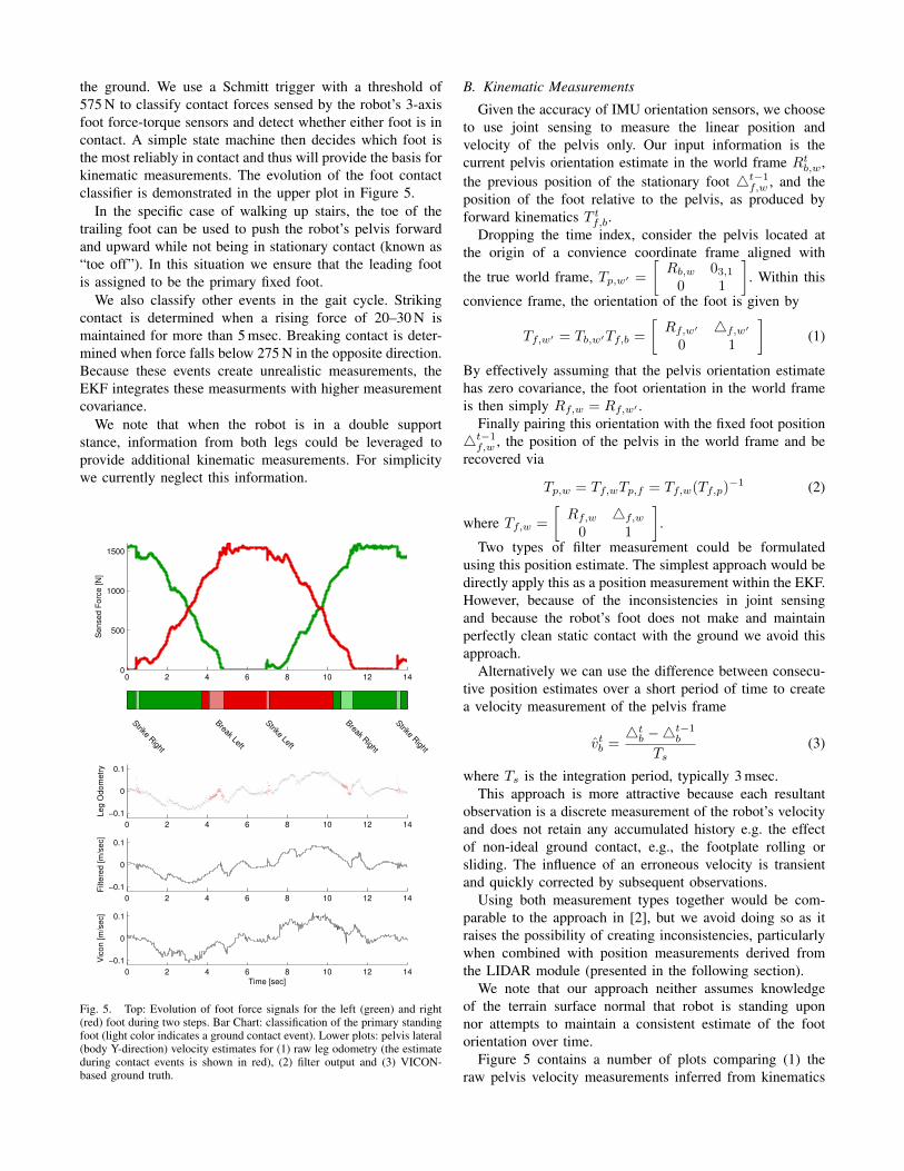
the ground. We use a Schmitt trigger with a threshold of575 N to classify contact forces sensed by the robot’s 3-axisfoot force-torque sensors and detect whether either foot is incontact. A simple state machine then decides which foot isthe most reliably in contact and thus will provide the basis forkinematic measurements. The evolution of the foot contactclassifier is demonstrated in the upper plot in Figure 5.

In the specific case of walking up stairs, the toe of thetrailing foot can be used to push the robot’s pelvis forwardand upward while not being in stationary contact (known as“toe off”). In this situation we ensure that the leading footis assigned to be the primary fixed foot.

We also classify other events in the gait cycle. Strikingcontact is determined when a rising force of 20–30 N ismaintained for more than 5 msec. Breaking contact is deter-mined when force falls below 275 N in the opposite direction.Because these events create unrealistic measurements, theEKF integrates these measurments with higher measurementcovariance.

We note that when the robot is in a double supportstance, information from both legs could be leveraged toprovide additional kinematic measurements. For simplicitywe currently neglect this information.

0 2 4 6 8 10 12 140

500

1000

1500

Se

nse

d F

orc

e [

N]

Strike Right

Break Left

Strike Left

Break Right

Strike Right

0 2 4 6 8 10 12 14

−0.1

0

0.1

Le

g O

do

me

try

0 2 4 6 8 10 12 14

−0.1

0

0.1

Filt

ere

d [

m/s

ec]

0 2 4 6 8 10 12 14

−0.1

0

0.1

Time [sec]

Vic

on

[m

/se

c]

Fig. 5. Top: Evolution of foot force signals for the left (green) and right(red) foot during two steps. Bar Chart: classification of the primary standingfoot (light color indicates a ground contact event). Lower plots: pelvis lateral(body Y-direction) velocity estimates for (1) raw leg odometry (the estimateduring contact events is shown in red), (2) filter output and (3) VICON-based ground truth.

B. Kinematic Measurements

Given the accuracy of IMU orientation sensors, we chooseto use joint sensing to measure the linear position andvelocity of the pelvis only. Our input information is thecurrent pelvis orientation estimate in the world frame Rt

b,w,the previous position of the stationary foot 4t−1

f,w , and theposition of the foot relative to the pelvis, as produced byforward kinematics T t

f,b.Dropping the time index, consider the pelvis located at

the origin of a convience coordinate frame aligned with

the true world frame, Tp,w′ =

[Rb,w 03,10 1

]. Within this

convience frame, the orientation of the foot is given by

Tf,w′ = Tb,w′Tf,b =

[Rf,w′ 4f,w′

0 1

](1)

By effectively assuming that the pelvis orientation estimatehas zero covariance, the foot orientation in the world frameis then simply Rf,w = Rf,w′ .

Finally pairing this orientation with the fixed foot position4t−1

f,w , the position of the pelvis in the world frame and berecovered via

Tp,w = Tf,wTp,f = Tf,w(Tf,p)−1 (2)

where Tf,w =

[Rf,w 4f,w

0 1

].

Two types of filter measurement could be formulatedusing this position estimate. The simplest approach would bedirectly apply this as a position measurement within the EKF.However, because of the inconsistencies in joint sensingand because the robot’s foot does not make and maintainperfectly clean static contact with the ground we avoid thisapproach.

Alternatively we can use the difference between consecu-tive position estimates over a short period of time to createa velocity measurement of the pelvis frame

v̂tb =4t

b −4t−1b

Ts(3)

where Ts is the integration period, typically 3 msec.This approach is more attractive because each resultant

observation is a discrete measurement of the robot’s velocityand does not retain any accumulated history e.g. the effectof non-ideal ground contact, e.g., the footplate rolling orsliding. The influence of an erroneous velocity is transientand quickly corrected by subsequent observations.

Using both measurement types together would be com-parable to the approach in [2], but we avoid doing so as itraises the possibility of creating inconsistencies, particularlywhen combined with position measurements derived fromthe LIDAR module (presented in the following section).

We note that our approach neither assumes knowledgeof the terrain surface normal that robot is standing uponnor attempts to maintain a consistent estimate of the footorientation over time.

Figure 5 contains a number of plots comparing (1) theraw pelvis velocity measurements inferred from kinematics

with (2) the output of our integrating filter and (3) thevelocity estimated from VICON motion capture. Typicalpelvis velocity standard deviations, measured when standingstill, are as follows:

• Raw incoming kinematics: 7.6 cm/sec• After joint level filtering: 2.3 cm/sec• After EKF integration: 1.4 cm/sec

V. LIDAR MEASUREMENTS

As illustrated in Figure 1, the robot is equipped with aMultisense SL sensor head designed by Carnegie Roboticswhich combines a fixed binocular stereo camera with aHokuyo UTM-30LX-EW planar LIDAR sensor mountedon a spindle that can rotate up to 30 RPM. (We typicallyoperate the device at 5 RPM to densely sample the terrainwhen walking). The LIDAR captures 40 scan lines of theenvironment per second, each containing 1081 range returnsout to a maximum range of 30 meters. The entire head canpitch up and down (powered by a hydraulic actuator) butcannot yaw or roll.

Our projection of LIDAR range returns as points in the3D workspace accounts for the robot’s motion, and moreimportantly, the spindle rotation during the 1/40 secondscanning period of the LIDAR’s internal mirror. Neglectingthis effect would result in mis-projections of returns to theside of the robot by as much at 2.5 m at the highest spindlerotation speed. Accurate projection also requires precisecalibration of the LIDAR sensor, as discussed in [8].

A. Contribution to Estimation

Our strategy is to use the LIDAR to continuously infer therobot’s position relative to a prior map while walking. Wecannot assume that the sensor is oriented horizontally [13],nor can we afford time to stop moving and perform static3D registration, e.g., using an Iterative Closest Point algo-rithm [14]. Instead we aim to incorporate information fromeach individual LIDAR scan into the state estimate using aGaussian Particle Filter, as originally described in [12].

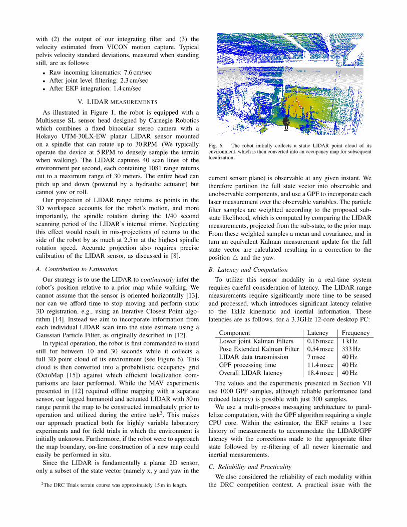
In typical operation, the robot is first commanded to standstill for between 10 and 30 seconds while it collects afull 3D point cloud of its environment (see Figure 6). Thiscloud is then converted into a probabilistic occupancy grid(OctoMap [15]) against which efficient localization com-parisons are later performed. While the MAV experimentspresented in [12] required offline mapping with a separatesensor, our legged humanoid and actuated LIDAR with 30 mrange permit the map to be constructed immediately prior tooperation and utilized during the entire task2. This makesour approach practical both for highly variable laboratoryexperiments and for field trials in which the environment isinitially unknown. Furthermore, if the robot were to approachthe map boundary, on-line construction of a new map couldeasily be performed in situ.

Since the LIDAR is fundamentally a planar 2D sensor,only a subset of the state vector (namely x, y and yaw in the

2The DRC Trials terrain course was approximately 15 m in length.

Fig. 6. The robot initially collects a static LIDAR point cloud of itsenvironment, which is then converted into an occupancy map for subsequentlocalization.

current sensor plane) is observable at any given instant. Wetherefore partition the full state vector into observable andunobservable components, and use a GPF to incorporate eachlaser measurement over the observable variables. The particlefilter samples are weighted according to the proposed sub-state likelihood, which is computed by comparing the LIDARmeasurements, projected from the sub-state, to the prior map.From these weighted samples a mean and covariance, and inturn an equivalent Kalman measurement update for the fullstate vector are calculated resulting in a correction to theposition 4 and the yaw.

B. Latency and Computation

To utilize this sensor modality in a real-time systemrequires careful consideration of latency. The LIDAR rangemeasurements require significantly more time to be sensedand processed, which introduces significant latency relativeto the 1kHz kinematic and inertial information. Theselatencies are as follows, for a 3.3GHz 12-core desktop PC:

Component Latency FrequencyLower joint Kalman Filters 0.16 msec 1 kHzPose Extended Kalman Filter 0.54 msec 333 HzLIDAR data transmission 7 msec 40 HzGPF processing time 11.4 msec 40 HzOverall LIDAR latency 18.4 msec 40 Hz

The values and the experiments presented in Section VIIuse 1000 GPF samples, although reliable performance (andreduced latency) is possible with just 300 samples.

We use a multi-process messaging architecture to paral-lelize computation, with the GPF algorithm requiring a singleCPU core. Within the estimator, the EKF retains a 1 sechistory of measurements to accommodate the LIDAR/GPFlatency with the corrections made to the appropriate filterstate followed by re-filtering of all newer kinematic andinertial measurements.

C. Reliability and Practicality

We also considered the reliability of each modality withinthe DRC competition context. A practical issue with the

inertial sensor is that the robot must be completely stationaryduring initialization. Boston Dynamics’ estimator requiresinitialization as soon as the robot is first powered on,typically with its feet solidly contacting the ground. Ourproposed estimator provides greater flexibility, as it canbe initialized at any point when the robot is standing anddeemed to be stationary.

While the time taken to construct the LIDAR map (10–30 sec) is a minor inconvenience, in all datasets and taskscenarios available to us there was sufficient stationarystructure within sensor range for localization to operatereliably. Since the algorithm uses measurements of the entireenvironment, movement of a few objects or people near therobot has no noticeable effect on performance. However, inscenarios containing substantial background motion (such asthe crowds attending the DRC Trials), special considerationmay be required to disregard portions of the map withsignificant activity.

Finally, while our preference has been to build a map froma single location and use it continuously while operating,in Section VII-B we demonstrate that the GPF localizationalgorithm is robust to non-encompassing maps as well.

VI. STEREO VISION

While the Multisense SL contains a stereo camera cap-turing 1-MPix images at up to 15 Hz with an 80◦ x 80◦

field of view, in this paper we do not focus on the useof vision within our state estimation. Figure 8 illustrateschallenging but realistic scenes from the DRC Trials —containing strong shadows, false feature detections, andabrupt lighting changes — all of which are detrimental tovision algorithms. Computational requirements and latencyare also not insignificant, so we have focused efforts to dateon exteroceptive measurements from LIDAR alone.

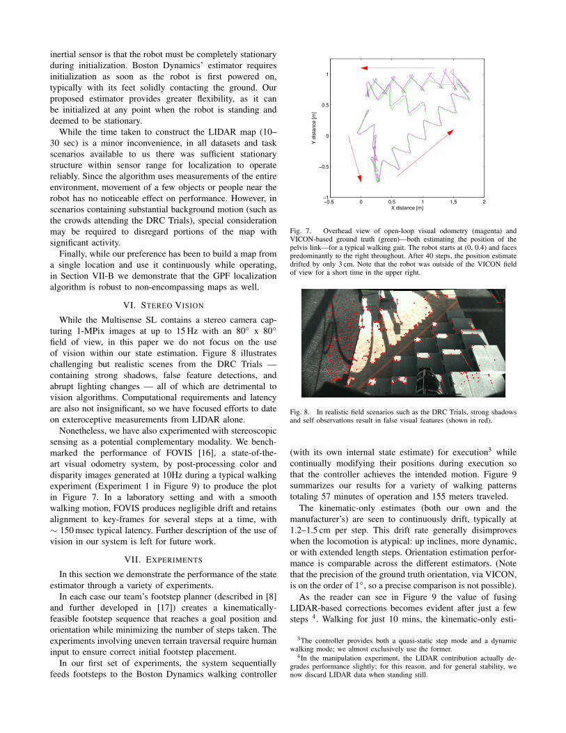
Nonetheless, we have also experimented with stereoscopicsensing as a potential complementary modality. We bench-marked the performance of FOVIS [16], a state-of-the-art visual odometry system, by post-processing color anddisparity images generated at 10Hz during a typical walkingexperiment (Experiment 1 in Figure 9) to produce the plotin Figure 7. In a laboratory setting and with a smoothwalking motion, FOVIS produces negligible drift and retainsalignment to key-frames for several steps at a time, with∼ 150 msec typical latency. Further description of the use ofvision in our system is left for future work.

VII. EXPERIMENTS

In this section we demonstrate the performance of the stateestimator through a variety of experiments.

In each case our team’s footstep planner (described in [8]and further developed in [17]) creates a kinematically-feasible footstep sequence that reaches a goal position andorientation while minimizing the number of steps taken. Theexperiments involving uneven terrain traversal require humaninput to ensure correct initial footstep placement.

In our first set of experiments, the system sequentiallyfeeds footsteps to the Boston Dynamics walking controller

−0.5 0 0.5 1 1.5 2−1

−0.5

0

0.5

1

X distance [m]

Y d

ista

nce

[m

]

Fig. 7. Overhead view of open-loop visual odometry (magenta) andVICON-based ground truth (green)—both estimating the position of thepelvis link—for a typical walking gait. The robot starts at (0, 0.4) and facespredominantly to the right throughout. After 40 steps, the position estimatedrifted by only 3 cm. Note that the robot was outside of the VICON fieldof view for a short time in the upper right.

Fig. 8. In realistic field scenarios such as the DRC Trials, strong shadowsand self observations result in false visual features (shown in red).

(with its own internal state estimate) for execution3 whilecontinually modifying their positions during execution sothat the controller achieves the intended motion. Figure 9summarizes our results for a variety of walking patternstotaling 57 minutes of operation and 155 meters traveled.

The kinematic-only estimates (both our own and themanufacturer’s) are seen to continuously drift, typically at1.2–1.5 cm per step. This drift rate generally disimproveswhen the locomotion is atypical: up inclines, more dynamic,or with extended length steps. Orientation estimation perfor-mance is comparable across the different estimators. (Notethat the precision of the ground truth orientation, via VICON,is on the order of 1◦, so a precise comparison is not possible).

As the reader can see in Figure 9 the value of fusingLIDAR-based corrections becomes evident after just a fewsteps 4. Walking for just 10 mins, the kinematic-only esti-

3The controller provides both a quasi-static step mode and a dynamicwalking mode; we almost exclusively use the former.

4In the manipulation experiment, the LIDAR contribution actually de-grades performance slightly; for this reason, and for general stability, wenow discard LIDAR data when standing still.

mators drift by as much as a meter while the LIDAR aidedapproach remains accurate to within a 2cm throughout.

A. Continuous Terrain Traversal

In an experiment of specific note, depicted in Figure 10,the robot traverses a set of cinder blocks that matchesthe terrain course from the December 2013 DRC Trials.The LIDAR-aided localization estimate remains accurate towithin 2 cm at all times, enabling the robot to continuouslywalk over the blocks. It can even execute this sequence inreverse to return to its exact starting position, despite havingno rear-facing sensors, because the forward-facing sensorskeep the robot so precisely localized. This forward-backwardtraversal was repeated 4 times in 12 minutes. By comparison,the kinematic-only estimates drift continuously, culminatingin a total of 0.8 m accumulated error, and would have causedthe robot to fall after its first few steps.

During the December 2013 DRC Trials, most teams exe-cuted the terrain course two steps at a time because of thisdrift (see [8] for our analysis of the task). Extrapolating fromthis experiment, the proposed algorithm can enable executionabout four times more quickly than was achieved in the DRCTrials.

B. Localization in Partial Maps

In a second noteworthy experiment, captured in a videoaccompanying this paper, we explored the performance ofthe estimator when the robot is not fully surrounded bythe prior map. The field of view of the LIDAR sensorroughly accommodates mapping the hemisphere in front ofthe robot from a single standing position. In this experimentthe robot first created a map from its starting pose and thenturned 90 degrees before walking for 12 minutes, such thata significant portion of the LIDAR data fell outside of themap. Localization performance (Experiment 2 in Figure 9)was much the same as in the other experiments, furtherdemonstrating the robustness of the proposed approach.

The likelihood function underlying the GPF is computedas the product of the likelihood of each LIDAR return in ascan. When a return falls far from an occupied cell of theOctoMap, an unobserved likelihood is applied to this return,resulting in stable performance despite a high percentage ofpotentially corruptive outlier measurements.

VIII. CONCLUSIONS

We have presented a probabilistic fusion algorithm forhumanoid state estimation and characterized the contributionof inertial, kinematic and LIDAR sensing to that estimate. Ofparticular note is that the approach supports continuous driftfree localization within a 3D LIDAR map, which we aimto use for enabling longer-term semi-autonomous operationof the BDI Atlas humanoid robot. A key result is thatour approach allows the robot to continuously walk overcomplex terrain while precisely achieving all of its footstepplacements, which was demonstrated in a variety of extendedexperiments and would not have been possible without theproposed algorithm.

0 2 4 6 8 10 120.8

1

1.2

1.4

Z h

eig

ht

[m]

0 2 4 6 8 10 12

−0.05

0

0.05

Z e

rro

r [m

]

0 2 4 6 8 10 12

0.1

0.2

0.3

XY

Z P

ositio

n E

rro

r [m

]

0 2 4 6 8 10 12−2

0

2

Ya

w E

rro

r [d

eg

]

Time [mins]

Fig. 10. Analysis of continuous and repeated traversal of the terrainillustrated in the upper image. In the upper plot, green is the VICONground truth; blue is the estimate provided by BDI; black incorporatesinertial and kinematic data and behaves similarly; magenta additionallyincorporates LIDAR and as a result remains accurately localized. A longer5-block traversal sequence (both forward and backward) can be seen in thesupplementary video accompanying this paper.

In future work we will focus on better characterizationof the joint angle biases so as to reduce the rate of kine-matic drift as well as incorporating vision as a contributingcomponent (Section VI).

A. Adaptations for Closed Loop Control

In parallel with these efforts, we have now adapted ourquadratic program-based walking controller [9] for use inplace of the manufacturer-provided controller. The stateestimator described here is being used directly in the 200Hzcontrol loop without modification. We also carry out in-dependent Kalman filtering of the 12 lower body jointsmeasurements, which was mentioned briefly above. As yet,we have not moved to integrate the LIDAR-based positioncorrection module into our real-time control.

A selection of videos showing the state estima-

XYZ drift Z drift Yaw drift0

0.2

0.4

0.6

0.81. Typical − 35m − 15 min

0

0.8

1.6

XYZ drift Z drift Yaw drift0

0.2

0.4

0.6

0.82. Typical − 37m − 12 min

0

0.4

0.8

XYZ drift Z drift Yaw drift0

0.1

0.2

0.3

0.4

0.53. Long Steps − 28m − 10 min

0

1.0

2.0

XYZ drift Z drift Yaw drift0

0.2

0.4

0.6

0.8

1

4. Dynamic − 7m − 2 min

0

0.6

1.2

XYZ drift Z drift Yaw drift0

0.01

0.02

0.03

0.04

0.05

0.065. Manip − 6m − 4 min

0

1.0

2.0

XYZ drift Z drift Yaw drift0

0.2

0.4

0.6

0.8

16. Blocks − 40m − 14 min

0

3.3

6.7

Fig. 9. Summary of localization accuracy for a variety of walking experiments. Position drift is measured with the left scale (in meters) and yaw driftwith the right scale (in degrees). Error (versus ground truth) of the BDI state estimator (blue), MIT’s kinematic-only (green) and closed-loop LIDAR (red)estimators are shown. Clockwise from upper left: 1: typical gait (15 cm forward steps), 2: typical gait with a partial map (see Section VII-B), 3: long steps(36 cm forward steps), 4: dynamic walking, 5: carrying out manipulation, 6: traversing the cinder block course in Figure 10.

tion combined with the walking controller, as well asall the developed source code, can be accessed atpeople.csail.mit.edu/mfallon/state-est

ACKNOWLEDGMENT

This work was supported by the Defense Advanced Re-search Projects Agency (via Air Force Research Laboratoryaward FA8750-12-1-0321). We thank the MIT DRC Teamfor their work on the overall humanoid system and AdamBry, Abe Bachrach and Dehann Fourie for development ofthe core estimation framework.

REFERENCES

[1] B. J. Stephens, “State estimation for force-controlled humanoid bal-ance using simple models in the presence of modeling error,” in IEEEIntl. Conf. on Robotics and Automation (ICRA), May 2011, pp. 3994–3999.

[2] X. Xinjilefu, S. Feng, W. Huang, and C. Atkeson, “Decoupled stateestimation for humanoids using full-body dynamics,” in IEEE Intl.Conf. on Robotics and Automation (ICRA), Hong Kong, China, 2014.

[3] M. Bloesch, M. Hutter, M. A. Hoepflinger, S. Leutenegger, C. Gehring,C. D. Remy, and R. Siegwart, “State estimation for legged robots -consistent fusion of leg kinematics and IMU,” in Robotics: Scienceand Systems (RSS), 2012.

[4] N. Rotella, M. Bloesch, L. Righetti, and S. Schaal, “State estimationfor a humanoid robot,” CoRR, vol. 1402.5450, 2014, IROS Submis-sion.

[5] S. Chitta, P. Vernaza, R. Geykhman, and D. Lee, “Proprioceptivelocalization for a quadrupedal robot on known terrain,” in IEEE Intl.Conf. on Robotics and Automation (ICRA), April 2007, pp. 4582–4587.

[6] O. Stasse, A. J. Davison, R. Sellaouti, and K. Yokoi, “Real-time3D SLAM for a humanoid robot considering pattern generator in-formation,” in IEEE/RSJ Intl. Conf. on Intelligent Robots and Systems(IROS), 2006.

[7] A. Hornung, K. M. Wurm, and M. Bennewitz, “Humanoid robotlocalization in complex indoor environments,” in IEEE/RSJ Intl. Conf.on Intelligent Robots and Systems (IROS), Taipei, Taiwan, October2010.

[8] M. Fallon, S. Kuindersma, S. Karumanchi, M. Antone, T. Schneider,H. Dai, C. P. D’Arpino, R. Deits, M. DiCicco, D. Fourie, T. T. Koolen,P. Marion, M. Posa, A. Valenzuela, K.-T. Yu, J. Shah, K. Iagnemma,R. Tedrake, and S. Teller, “An architecture for online affordance-basedperception and whole-body planning,” J. of Field Robotics, 2014.

[9] S. Kuindersma, F. Permenter, and R. Tedrake, “An efficiently solvablequadratic program for stabilizing dynamic locomotion,” in IEEE Intl.Conf. on Robotics and Automation (ICRA), Hong Kong, China, June2014.

[10] D. C. Moore, A. S. Huang, M. Walter, E. Olson, L. Fletcher,J. Leonard, and S. Teller, “Simultaneous local and global state es-timation for robotic navigation,” in IEEE Intl. Conf. on Robotics andAutomation (ICRA), 2009.

[11] E. Marder-Eppstein, E. Berger, T. Foote, B. Gerkey, and K. Konolige,“The Office Marathon: Robust navigation in an indoor office environ-ment,” in IEEE Intl. Conf. on Robotics and Automation (ICRA), May2010.

[12] A. Bry, A. Bachrach, and N. Roy, “State estimation for aggressiveflight in GPS-denied environments using onboard sensing,” in IEEEIntl. Conf. on Robotics and Automation (ICRA), 2012, pp. 1–8.

[13] F. Dellaert, D. Fox, W. Burgard, and S. Thrun, “Monte Carlo lo-calization for mobile robots,” in IEEE Intl. Conf. on Robotics andAutomation (ICRA), May 1999.

[14] P. J. Besl and N. D. McKay, “A method for registration of 3-D shapes,”IEEE Trans. Pattern Anal. Machine Intell., vol. 14, no. 2, pp. 239–256,1992.

[15] K. M. Wurm, A. Hornung, M. Bennewitz, C. Stachniss, and W. Bur-gard, “OctoMap: A probabilistic, flexible, and compact 3D maprepresentation for robotic systems,” in Proc. of the ICRA 2010 Work-shop on Best Practice in 3D Perception and Modeling for MobileManipulation, Anchorage, AK, USA, May 2010.

[16] A. Huang, A. Bachrach, P. Henry, M. Krainin, D. Maturana, D. Fox,and N. Roy, “Visual odometry and mapping for autonomous flightusing an RGB-D camera,” in Proc. of the Intl. Symp. of RoboticsResearch (ISRR), Flagstaff, USA, Aug. 2011.

[17] R. L. Deits and R. Tedrake, “Computing large convex regions ofobstacle-free space through semi-definite programming,” in Workshopon the Algorithmic Fundamentals of Robotics (WAFR), Istanbul,Turkey, Aug. 2014.