Energy Efficiency in Humanoid Robots A preliminary study on a humanoid torso

L. De Michieli, F. Nori, G. Sandini Robotics Brain and Cognitive Research Department

Fondazione Istituto Italiano di Tecnologia - IIT Genova, Italy

lorenzo.demichieli@iit.it, francesco.nori@iit.it

A Pini Prato DIMSET Department

Università degli Studi di Genova Genova, Italy

salabi@unige.it

Abstract— This work is about the energy analysis of a humanoid robotic arm, seen as complex energy chain. We developed a simulation platform suitable for modelling the kinematics, dynamics, and energy balances of a real humanoid robotic arm. The model was validated by an accurate comparison with the real robot. Then, we performed a first compared study of the motion dynamics of the simulated robot arm and the energy flowing across its energy converters, with respect to a set of different motion control strategies. Moreover, we conducted a preliminary investigation on the possibility of saving and recovering energy during robot motion.

Keywords: motion controls, energy efficiency, humanoid robot.

I. INTRODUCTION This work intends to provide an energy analysis of a state

of art humanoid robot [1] according to some of the methodologies which derive from research on distributed energy systems and energy converters, by developing suitable instruments and methods [6], [7], [8]. According to our approach, humanoid robots are represented as isolated energy systems comprising a number of energy converters which are interconnected so as to produce the expected task.

Typically, humanoid robots are equipped with at least one primary converter (for instance, a battery or an internal combustion engine), followed by other converters aimed at transforming the electric energy into mechanical energy. Usually these are the electric motors. At the end of the energy chain there are those converters that have direct interaction with the environment, that is, the robot workspace. They are the robot actuators such as tactile sensors, manipulators, pincers, cameras, human-like hands. Finally, all the energy converters are interconnected within a power distribution net. A central control unit is expected to manage the distribution net and to dispatch the appropriate power to each single converter in order to carry out the desired mission (i.e. goal oriented task).

The problem of humanoid robots autonomy, and therefore of energy efficiency is remarkable [9], especially in view of assigning them increasingly complex tasks. Besides the search for more performing energy converters, a solution can be carried out studying the structural characteristics as well as the dynamics of the robot system, aimed at minimizing its energy consumption with respect to a given mission [3], [10], [12]. Accordingly, the energy chain must be analysed in terms of

single converters, especially concerning effects that the possible variations of typology and topography of the intermediate converters produce on the primary converter, for a given task. Moreover, in case the structure of the robot is determined in terms of configuration and category of the actuators, and the desired mission is identified, it is important to conduct an energy analysis of the effects of the motion controls and cognitive process of the robot. Indeed, given a task, the overall efficiency of the robot is strongly dependent on the actions that the robot decides to carry out [9] [11].

This type of analysis requires the definition and use of an appropriate physical model that resolves the dynamics of each converter, including the effects of both the internal and the external forces acting on it, such as friction, gravity, inertial effects. The characterization of the energy chain allows to locally identify energy losses and possible energy savings. As an example, it is possible to calculate the backward energy flows occurring when the robot arm moves under the effect of gravity, or when it is driven by external forces.

We believe that the correlation of the energy aspects of a humanoid robot with its motion dynamics and its control strategies can represent an effective approach to individuate an energy efficient design of the system.

II. OBJECTIVES Our primary objective is to develop a simulation platform

suitable for modelling the kinematics, dynamics, and energy balance of a real humanoid robotic arm. We want to provide a flexible simulator that allow us to reproduce the elements of the robot energy chain in terms of mechanical and electrical components, and to simulate a large number of motion control strategies. A further aim is to present a correlation between the motion dynamics of the robot arm and the energy flowing through its converters, with respect to a set of different motion control strategies. In particular, three motion control logics have been developed and compared with the one which currently drives the real robotic arm. We simulated goal oriented tasks in order to obtain a local and a global study of the dynamics, the kinematics and the energy related parameters of the system.

III. DESCRIPTION OF ROBOT JAMES James is a humanoid robotic platform which is developed

by the University of Genoa in collaboration with the Italian

Institute of Technology. The robot is equipped with moving eyes, neck, arm and hand, and a rich set of sensors, enabling proprioceptive, kinesthetic, tactile and visual sensing.

Fig. 1 The humanoid robot James at IIT

James consists of 22 Degrees of Freedom (DOF), actuated by a total of 23 motors, whose torque is transmitted to the joints by belts and stainless-steel tendons. The head is equipped with two eyes, which can pan and tilt independently (4 DOFs), and is mounted on a 3-DOF neck, which allows the movement of the head as needed in the 3D rotational space. The arm has 7 DOFs: three of them are located in the shoulder, one in the elbow and three in the wrist. The hand has five fingers. Each of them has three joints. The robot arm, which is the object of the simulation described herein, is basically composed of four main parts: the shoulder, the upper arm, the forearm, and the hand. In the following a brief description of the single mechanical parts is given.

A. The shoulder The shoulder consists of three successive rotations Jϕ ,

called pitch Jpϕ , yaw J

yϕ , and roll Jrϕ respectively (Fig. 2).

Fig. 2 The kinematic chain of James’s arm (right). The systems of reference herein reported are chosen according to the Denavit Hartemberg notation. Left figure: graphical representation of James software model.

The abduction (yaw) rotation is divided along two mechanically coupled joints having rotation corresponding to a sequence of two identical rotations /2

Jyϕ around two parallel

axes. Indeed, a mechanical tight coupling forces the two angles of rotation to be equal.

James arm is actuated by a set of 4 DC Faulhaber motors which we will call M1, M2, M3, M4. Each motor is equipped with a planetary gearhead and it is coupled with an incremental magnetic encoder to calculate the relative position

of the links. A table of the motors specifications is reported herein:

TABLE I MOTORS MODELS DRIVING THE 4 DOF ROBOT ARM

# DC MOTOR (Faulhaber) GEARHEAD (Faulhaber) M1 3242G012CR 32/3, reduction ratio: 246:1 M2 3242G012CR 32/3, reduction ratio: 246:1 M3 2342S012CR 26/1, reduction ratio: 66:1 M4 2224U012SR 23/1, reduction ratio: 246:1

While the forearm rotation J

eϕ about the elbow axis is actuated by the motor M4 only, the rotations of the first three links about the yaw, pitch, and roll axis, are caused by the simultaneous actuation of the motors M1, M2, and M3.

Indicating with ( )M M M Mp y r eϕ ϕ ϕ ϕ the shafts’ angles of the

motors M1, M2, M3, M4, the relation between these angles and the rotation angles yaw pitch and roll can be written as:

[ ] [ ]T TJ J J M M Mp y r p y rDϕ ϕ ϕ ϕ ϕ ϕ= (1)

where

1

2462 2

246 2461 2 1

246 246 66

0 00.555 0 D

⎡ ⎤= −⎢ ⎥

⎢ ⎥⎣ ⎦ (2)

The numerical values of D derives from the values of the coupling factors between the position of motors and the position of links and the reduction ratios of the gearboxes.

IV. DESCRIPTION OF THE SIMULATOR The simulator has been designed with the aim of being

fully configurable with respect to the mechanical and electrical specifications, so that any change in the kinematic of the robot, in the motors and in the robot dynamical characteristics can be easy to implement and managed.

The simulator can be divided in the following 5 groups: Mechanical apparatus (A); Motors & transmission (B); Motion control strategies (C); Energy analysis module (D). The simulator requires the use of two different software packages: a professional mobile robot simulation software named ‘Webots’ and the well known ‘Matlab’ package. These two software have been linked by means of tcp/ip like communication protocol in order to obtain one single simulation environment. Group A and part of group C have been developed by using Webots, while B and D have been developed in Matlab code. Motor controls and most of the custom physics simulation libraries have been implemented in C language.

A. The Mechanical Apparatus The model has been schematised as a set of rigid

multibody system consisting of a set of rigid objects joined together by joints and ending with an end-effector (the hand). The whole kinematic chain of the arm has 4 DOF and is mechanically connected to the upper torso from one side, and to the other side it is rigidly attached to the robot hand. The following Fig. 3 shows the simulated James layout.

B. The DC Motors and the Transmission

The motor models are based on the well known equations describing a dc motor. From the values of the electrical and mechanical constants of every motor, given an input voltage V, current I and the output torque Mτ for each of the motors are calculated. Then, according to the motor to joints mechanical coupling (Fig. 3), the torques Mτ produced by the motors are converted into joint torques Jτ , by means of a change of coordinates from (1), resulting J T MDτ τ−= .

L1

L3L4

ϕp ϕy/2

ϕr

ϕe

ϕy/2

M1

M2

M3

M4

T1

T2

T3

T4

Fig. 3 Transmission layout. Angles are relative to the joints positions.

The simulator reproduces also four transmissions lines T1, T2, T3, T4 which bring the mechanical power from the converters output (the dc motors shaft after the gearhead) to the links. Each transmission is affected by power losses which are modeled like a pure viscous friction. The modeled friction originally derives from the motion of each link according to the equation:

9.8 0 0 00 10.2 0 0 ; 0 0 2.5 00 0 0 2.8

JF E Eτ ϕ

⎡ ⎤⎢ ⎥= = ⎢ ⎥⎢ ⎥⎣ ⎦

(3)

where Jϕ is the time derivative of the joint angular position vector and E is the diagonal matrix of the estimated viscous friction coefficients expressed in [Ns/rad]. According to (4), the resulting torque applied to the ith link is finally calculated as:

J MFDτ τ τ−Τ= − (5)

C. Motion controller It is aimed at driving the motors to move the robot arm

according to a series of constraints on kinematics, dynamics and efficiency, which are determined by the given mission.

Motion control stage

ϕref

PIDV

Pre-motion stageOptimal control solver

Motors

Dynamics of the Arm

τ

To motors

To Joints

ϕactual

User defined mission

parameters

Fig. 4 Scheme of the Motion Controller module.

It is composed of two stages: the pre-motion stage and the motion control stage. In the pre-motion stage the user can define the mission of the arm in terms of duration, initial and boundary conditions of the motion, energy parameters. Then, the system calculates the reference trajectories for the arm, i.e. the trajectories that the arm should carry out in order to accomplish the given mission. These trajectories are evaluated as solutions to optimal control problems which are chosen by the user. The Motion Controller calculates both the forward and the inverse kinematic (based on the downhill simplex method of Nelder and Mead [15]).

The four control strategies herein implemented can be described as solutions of an optimal control problem subject to the minimization of a cost function ξ, such as:

{0

0 0

min ( ( ), ( ), )

( ) ( ( )) ( ( )) ( )subject to ( )

ftu

tJ x t u t t dt

x t f x t g x t u tx t x

ξ⎧ =⎪⎪⎨

= +⎪=⎪⎩

∫ (6)

The Motion control module calculates u(t) that minimize the functional, and the state of the system x(t) accordingly. Then, the values ( ) ( ( ), ( ))J Jx t t tϕ ϕ= are used as reference trajectories that the arm will have to follow.

The Minimum Jerk in the Cartesian space (MJe), that is the Cartesian end-effector position referred to the inertial base frame S – Fig. 2, has the functional ξ equal to:

( )2 2 23 3 3

3 3 3( ), ( ), ( ) d x d y d zx t y t z t dt dt dtξ ⎛ ⎞ ⎛ ⎞ ⎛ ⎞= + +⎜ ⎟ ⎜ ⎟ ⎜ ⎟⎝ ⎠ ⎝ ⎠ ⎝ ⎠

(7)

where (x, y, z) are the hand effector coordinates. Similarly, the Minimum Jerk in joint space coordinates (MJq) is characterized by:

( )23

3( ) dt dtξ ⎛ ⎞= ⎜ ⎟⎝ ⎠

φφ (8)

where φ is the vector of the joints coordinates. The Minimum Torque Change (MTC) function indeed is

related with total torque change during the movement, which is given by:

( )2

( ) dt dtξ = ττ (9)

where τ is the vector of torques acting on the joints. The Minimum Torque (MT) cost function is given by:

( ) 2( )tξ =τ τ (10)

where τ is the vector of torques acting on the joints.

D. Energy Analysis module This module is designed to provide the information

relative to the energy flows occurring inside the energy chain, it collects the energy relevant parameters within specified subsystems or control volumes, and within a given observation time. More specifically, the following control volumes have been identified (Fig. 5): single motor; motors

group; power transmission of a single motor; overall power transmission; single link of the arm; links group (complete robot arm); whole system. The power supplier unit is a strictly one-way energy converter, while the energy inside the rest of the chain passes through the components in both directions: it flows towards the links and, in principle, it can return back towards the mechanical transmission up to the power supplier.

Fig. 5 Energy chain diagram. Control volumes are evidenced by dashed lines.

This may happen, for example, under the effect of external forces, such as the weight of a load held by the robot, or the gravity acting on the arm. In general, due to external forces or to the mechanical coupling of the converters, given a particular mission and a control time, some of the converters acts like motors, while others behave like voltage generators. In view of that, let’s consider a volume of control crossed by energy flows in both directions in which there are energy losses. We define the “input” of a given volume of control as the frontier from which the net energy flow, calculated over the whole control time T, enters the volume, and the “output” as the frontier crossed by the energy flow leaving such volume.

With reference to Fig. 6, given a control time T and a volume of control having frontiers ‘p’ and ‘q’ we define net energy flows as:

( ) ( ) , ( ) ( )p p p q q qf b f bW W W W W W= − = − (11)

where: ( )pfW = forward energy to ‘p’; ( )q

fW = forward energy to ‘q’; ( )p

qW = backward energy from ‘p’; ( )qbW =

backward energy from ‘q’.

According to the present definitions, the frontier ‘p’ will be called ‘input’ frontier, while ‘q’ will be called the ‘output’ frontier of the volume of control. Now it is possible to unambiguously define the efficiency associated to a determined control volume and a determined control period.

( )p

fW ( )q

fW

( )pb

W ( )qb

W

Losses

q p Wp Wq

Fig. 6 Two-way energy converter

The following expressions of “forward” ( ) fη and “backward” ( )bη average converter efficiency are applicable

when the energy flow across the converter is time-dependent and its internal energy is negligible as compared to the flow passing through in the control time:

( ) ( )( ) ; ( )( ) ( )out f in b

f bin f out b

W WW Wη η= = (12)

The effective average efficiency of the converter is defined as:

( ) ( )( ) ( )

out f out b

in f in b

W WW Wη −

=−

(13)

The backward energy ratio R is defined as the ratio between the backward energy module returning up to the converter from the output frontier and the direct energy output:

( )( )

out b

out f

WR W= (14)

From (13) and (14), the generalized form of the average efficiency of the i-th converter is:

( ) ( ) ( )11

ii i

i i i ff b

RR

η ηη η−=

− (15)

Equation (15) shows clearly that the efficiency of the converter does not depend on its intrinsic performances only, i.e. forward and backward efficiency, but also on the backward energy ratio R, i.e. on the way the converter is used: the more energy is returning, the less the converter is in fact efficient, either it behaves like a motor either like a generator.

In the light of the aforementioned concepts, the energy balance of the robot has been derived by integrating over time the estimated power flowing through each component (dc motors, transmission, links). Considering (16), from the left to the right we have the equations for input power to motor Mi, output power of the motor Mi, output power of the transmission Ti, and output power of the link Li.

; ; ; Mi Mi Mi Mi Ti Ti Mi Ji Ji Jiin Mi Mi out out outP V I P P Pτ ϕ τ ϕ τ ϕ= = = = (16)

The quantities VMi and IMi are the input voltage to motor Mi and the current circulating into Mi respectively, while Tiτ is the torque exerted by transmission Ti. We also considered that Mi

outP is equal to the input power to transmission Ti (Fig. 5).

V. VALIDATION The validation has been conducted in four phases: the

parametric identification of the motors running inside the James arm, the tuning of the simulated motors on the base of the measured data, the observation of the dynamic of the arm during a set of simple movements and the tuning of the friction affecting the motors transmissions inside the robot James.

VI. SIMULATED MISSIONS AND ENERGY BALANCE The simulated missions consisted in reaching tasks, in

compliance of predefined constraints in time, space and forces. Each goal oriented task has been repeated for each of the four above described control strategies.

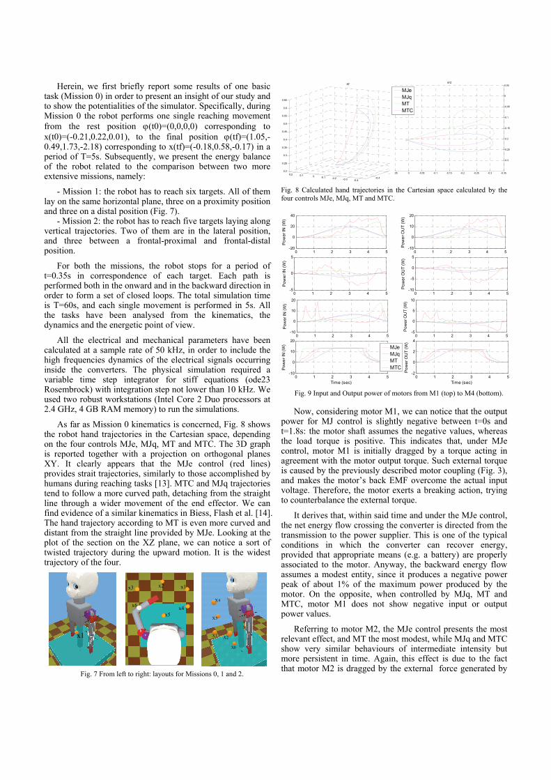
Herein, we first briefly report some results of one basic task (Mission 0) in order to present an insight of our study and to show the potentialities of the simulator. Specifically, during Mission 0 the robot performs one single reaching movement from the rest position ϕ(t0)=(0,0,0,0) corresponding to x(t0)=(-0.21,0.22,0.01), to the final position ϕ(tf)=(1.05,-0.49,1.73,-2.18) corresponding to x(tf)=(-0.18,0.58,-0.17) in a period of T=5s. Subsequently, we present the energy balance of the robot related to the comparison between two more extensive missions, namely:

- Mission 1: the robot has to reach six targets. All of them lay on the same horizontal plane, three on a proximity position and three on a distal position (Fig. 7).

- Mission 2: the robot has to reach five targets laying along vertical trajectories. Two of them are in the lateral position, and three between a frontal-proximal and frontal-distal position.

For both the missions, the robot stops for a period of t=0.35s in correspondence of each target. Each path is performed both in the onward and in the backward direction in order to form a set of closed loops. The total simulation time is T=60s, and each single movement is performed in 5s. All the tasks have been analysed from the kinematics, the dynamics and the energetic point of view.

All the electrical and mechanical parameters have been calculated at a sample rate of 50 kHz, in order to include the high frequencies dynamics of the electrical signals occurring inside the converters. The physical simulation required a variable time step integrator for stiff equations (ode23 Rosembrock) with integration step not lower than 10 kHz. We used two robust workstations (Intel Core 2 Duo processors at 2.4 GHz, 4 GB RAM memory) to run the simulations.

As far as Mission 0 kinematics is concerned, Fig. 8 shows the robot hand trajectories in the Cartesian space, depending on the four controls MJe, MJq, MT and MTC. The 3D graph is reported together with a projection on orthogonal planes XY. It clearly appears that the MJe control (red lines) provides strait trajectories, similarly to those accomplished by humans during reaching tasks [13]. MTC and MJq trajectories tend to follow a more curved path, detaching from the straight line through a wider movement of the end effector. We can find evidence of a similar kinematics in Biess, Flash et al. [14]. The hand trajectory according to MT is even more curved and distant from the straight line provided by MJe. Looking at the plot of the section on the XZ plane, we can notice a sort of twisted trajectory during the upward motion. It is the widest trajectory of the four.

x6

x2 x1

x4 x5

x3

X0

X1 X2

X3

X4

Fig. 7 From left to right: layouts for Missions 0, 1 and 2.

-0.4

-

-0.4-0.3-0.2-0.100.10.20.2

0.25

0.3

0.35

0.4

0.45

0.5

0.55

0.6

0.65

XZ

-0.3

-0.25

-0.2

-0.15

-0.1

-0.05

0

0.05

-0.35-0.3-0.25-0.2-0.15-0.1-0.050.05

XYZ

MJheMJqMTMTC

Fig. 8 Calculated hand trajectories in the Cartesian space calculated by the four controls MJe, MJq, MT and MTC.

0 1 2 3 4 5-20

0

20

40

Pow

er IN

(W)

0 1 2 3 4 5-10

0

10

20

Pow

er O

UT

(W)

0 1 2 3 4 5-5

0

5

Pow

er IN

(W)

0 1 2 3 4 5-10

-5

0

5

Pow

er O

UT

(W)

0 1 2 3 4 5-10

0

10

20

Pow

er IN

(W)

0 1 2 3 4 5-5

0

5

10

Pow

er O

UT

(W)

0 1 2 3 4 5-10

0

10

20

Pow

er IN

(W)

Time (sec)0 1 2 3 4 5

-2

0

2

4

Pow

er O

UT

(W)

Time (sec) Fig. 9 Input and Output power of motors from M1 (top) to M4 (bottom).

Now, considering motor M1, we can notice that the output power for MJ control is slightly negative between t=0s and t=1.8s: the motor shaft assumes the negative values, whereas the load torque is positive. This indicates that, under MJe control, motor M1 is initially dragged by a torque acting in agreement with the motor output torque. Such external torque is caused by the previously described motor coupling (Fig. 3), and makes the motor’s back EMF overcome the actual input voltage. Therefore, the motor exerts a breaking action, trying to counterbalance the external torque.

It derives that, within said time and under the MJe control, the net energy flow crossing the converter is directed from the transmission to the power supplier. This is one of the typical conditions in which the converter can recover energy, provided that appropriate means (e.g. a battery) are properly associated to the motor. Anyway, the backward energy flow assumes a modest entity, since it produces a negative power peak of about 1% of the maximum power produced by the motor. On the opposite, when controlled by MJq, MT and MTC, motor M1 does not show negative input or output power values.

Referring to motor M2, the MJe control presents the most relevant effect, and MT the most modest, while MJq and MTC show very similar behaviours of intermediate intensity but more persistent in time. Again, this effect is due to the fact that motor M2 is dragged by the external force generated by

MJeMJqMTMTC

x1

MJeMJqMTMTC

the load and the coupling with M1 and M3. The event is not negligible since it dominates the dynamics of the converter under all the control strategies for a large part of the motion. It derives that the net energy flowing across motor M2 is in average directed backwards from the transmission to the power supplier. Accordingly, the calculated average efficiency confirms that the M2 behaves as a generator under MJe, MJq and MTC controls, with an efficiency η equals to 0.19, 0.44 and 0.43 respectively.

As far as M3 is concerned, while voltage, current, and consequently the input power, are positive for most of the motion, the output power is in general negative. More precisely, it assumes small values, comprised between zero and P=-1.5W for MT, MTC, MJq, while for MJe it is positive in the first half of the motion, with peaks of ±5W. This effect is mainly due to the gravity acting on the arm, particularly on the forearm.

Motor M4 presents evidences of affording a full load for all the control strategies between t=1s and t=3.8s. The average efficiency over the control time for the motor M4 depends on the adopted control strategy rather weakly: all the mean efficiency varies from 17% for MJe up to 19% for MJq, while MT provides an average efficiency of 17%, and MTC gives 18%.

E. Efficiency and Energy Balance for Missions 1 & 2 Considering the most relevant energy related parameters

which have been calculated during Missions 1 and 2, we can infer that the highest system efficiency is provided by the MT, whereas the lowest average efficiency derives from MTC and MJe. The last two provide quasi identical values, about 15% lower than MT (Fig. 10). However, MT, together with MJe, seems to be the most energy consuming control, since it requires roughly 20% more energy than MJq and MTC (Fig. 10). It is also noteworthy that MT produces the worst trajectories considering the goal of the two missions. Indeed, MT, trajectories in the Cartesian space are noticeably curved and widely diverging from desirable straight line paths. On the other hand, it has been estimated that the control strategy producing the best trajectories, always with respect to their linearity, is MJe, which shows a higher efficiency than MTC and MJq, but requires more energy.

6,00

7,00

8,00

9,00

10,00

11,00

12,00

MJe MJq MTC MT

Energy efficiency [%]

522473 470

562

270218 220

258

0

100

200

300

400

500

600

MJe MJq MTC MT

Input Energy [J]

Fig. 10 average chain efficiencies calculated for missions 1 and 2

VII. CONCLUSIONS According to the simulation results, the control strategy

currently implemented on the real robot James (i.e. MJq) seems to be poorly efficient. Moreover, the average backward

energy ratio of MJq (Fig. 11) calculated for both the two missions, is maximum for MJq.

0,0000,0100,0200,0300,0400,0500,0600,0700,0800,0900,100

MJe MJq MTC MT

Backward Energy Ratio R

Mission 1

Mission 2

Fig. 11 Average system efficiencies calculated for missions 1 and 2

Thus, at least in principle, MJq may assure the largest amount of energy recovery, provided that appropriate accumulators and hardware adaptations are added to the real robot. This first study is aimed at exploring a possible approach for helping the understanding of the energy balance of robots in correlation with their motion controls and their mechanical constraints. Further studies on this topic might, for example, conduct to the design of energy recovery systems and to the exploration of energy efficient motion strategies.

ACKNOWLEDGMENT Work supported by EC Project IST-004370 RobotCub.

REFERENCES [1] L Jamone, G Metta, F Nori, G Sandini “James: A Humanoid Robot

Acting over an Unstructured World”- Humanoid Robots, 6th IEEE-RAS International Conference, 2006.

[2] O. Khatib et al., “Robots in Human Environments”, Stanford University. 2000.

[3] W. Schiehlen, “Energy-optimal design of walking machines”, Multibody System Dynamics, pp. 129-141, 2005.

[4] I. Ieropoulos, C. Melhuish, W. Aberystwyth “Imitating Metabolism: Energy Autonomy in Biologically Inspired Robotics”, Proc. of the AISB '03, 2003, pp. 191-194.

[5] E. Todorov, “Optimality principles in sensorimotor control”, Nature Neuroscience, Vol. 7, p. 907-915.

[6] A. Pini-Prato, M. Repetto, G. Vandelli, “Hybrid-series vehicle mathematical simulation model”, Trans. of Wessex Institute IX, 2003.

[7] G.L Berta, A. Pini Prato, “Series-Hybrid Power Trains: Design Criteria”, Proc. XXV FISITA Congress, BiJin 1994.

[8] G.L. Berta, A. Pini Prato, Bolfo F., “On Road Testing Hybrid Vehicles”, Int. Symposium on Automotive Technology and Automation, 1993.

[9] E. Todorov et al., “Optimal control methods suitable for biomechanical systems”, Proc. of the 25th Annual International Conference of the IEEE Engineering in Biology and Medicine Society, 2003.

[10] Y. Mei et al. “Deployment strategy for mobile robots with energy and timing constraints”. Proc. of the IEEE International Conference on Robotics and Automation, Barcelona, 2005. pp. 2816–2821.

[11] M. Kawato, “Internal models for motor control and trajectory planning”, Current Opinion in Neurobiology, pp. 718-727, 1999.

[12] S. Collins, A. Ruina, R. Tedrake, M. Wisse “Efficient Bipedal Robots Based on Passive-Dynamic Walkers”, Science, vol. 307, 1082 , 2005.

[13] Morasso, P. “Spatial control of arm movements“, Experimental Brain Research, Vol. 42, 1981, pp. 223-227

[14] Biess, Nagurka, Flash, “Simulating discrete and rhythmic multi-joint human arm movements by optimization of nonlinear performance indices”, Biological Cybernetics, Vol. 95, 2006, pp. 31-35.

[15] Press, William H., et al. “Numerical Recipes 3rd Edition: The Art of Scientific Computing”, Ney York Cambridge University Press, 2007.

Mission 1

Mission 2