generation of whole-body motion for humanoid robots
TRANSCRIPT
HAL Id: tel-01134313https://tel.archives-ouvertes.fr/tel-01134313
Submitted on 23 Mar 2015
HAL is a multi-disciplinary open accessarchive for the deposit and dissemination of sci-entific research documents, whether they are pub-lished or not. The documents may come fromteaching and research institutions in France orabroad, or from public or private research centers.
L’archive ouverte pluridisciplinaire HAL, estdestinée au dépôt et à la diffusion de documentsscientifiques de niveau recherche, publiés ou non,émanant des établissements d’enseignement et derecherche français ou étrangers, des laboratoirespublics ou privés.
Generation of the whole-body motion for humanoidrobots with the complete dynamics
Oscar Efrain Ramos Ponce
To cite this version:Oscar Efrain Ramos Ponce. Generation of the whole-body motion for humanoid robots with thecomplete dynamics. Robotics [cs.RO]. Universite Toulouse III Paul Sabatier, 2014. English. �tel-01134313�

Christine CHEVALLEREAU: Directeur de Recherche, École Centrale de Nantes, France
Francesco NORI: Researcher, Italian Institute of Technology, Italy
Patrick DANÈS: Professeur des Universités, Université de Toulouse III, France
Ludovic RIGHETTI: Researcher, Max-Plank-Institute for Intelligent Systems, Germany
Nicolas MANSARD: Chargé de Recherche, LAAS-CNRS, France
Philippe SOUÈRES: Directeur de recherche, LAAS-CNRS, France
Yuval TASSA: Researcher, University of Washington, USA
Abstract
This thesis aims at providing a solution to the problem of motion generation for humanoidrobots. The proposed framework generates whole-body motion using the complete robot dy-namics in the task space satisfying contact constraints. This approach is known as operational-space inverse-dynamics control. The specification of the movements is done through objectivesin the task space, and the high redundancy of the system is handled with a prioritized stack oftasks where lower priority tasks are only achieved if they do not interfere with higher priorityones. To this end, a hierarchical quadratic program is used, with the advantage of being ableto specify tasks as equalities or inequalities at any level of the hierarchy. Motions where therobot sits down in an armchair and climbs a ladder show the capability to handle multiplenon-coplanar contacts.
The generic motion generation framework is then applied to some case studies using HRP-2and Romeo. Complex and human-like movements are achieved using human motion imita-tion where the acquired motion passes through a kinematic and then dynamic retargetingprocesses. To deal with the instantaneous nature of inverse dynamics, a walking pattern gen-erator is used as an input for the stack of tasks which makes a local correction of the feetposition based on the contact points allowing to walk on non-planar surfaces. Visual feedbackis also introduced to aid in the walking process. Alternatively, for a fast balance recovery, thecapture point is introduced in the framework as a task and it is controlled within a desiredregion of space. Also, motion generation is presented for CHIMP which is a robot that needsa particular treatment.
Résumé
Cette thèse propose une solution au problème de la génération de mouvements pour les robotshumanoïdes. Le cadre qui est proposé dans cette thèse génère des mouvements corps-completen utilisant la dynamique inverse avec l’espace des tâches et en satisfaisant toutes les con-traintes de contact. La spécification des mouvements se fait à travers objectifs dans l’espacedes tâches et la grande redondance du système est gérée avec une pile de tâches où les tâchesmoins prioritaires sont atteintes seulement si elles n’interfèrent pas avec celles de plus hautepriorité. À cette fin, un QP hiérarchique est utilisé, avec l’avantage d’être en mesure de pré-ciser tâches d’égalité ou d’inégalité à tous les niveaux de la hiérarchie. La capacité de traiterplusieurs contacts non-coplanaires est montrée par des mouvements où le robot s’assoit surune chaise et monte une échelle.
Le cadre générique de génération de mouvements est ensuite appliqué à des études de casà l’aide de HRP-2 et Romeo. Les mouvements complexes et similaires à l’humain sont obtenusen utilisant l’imitation du mouvement humain où le mouvement acquis passe par un processuscinématique et dynamique. Pour faire face à la nature instantanée de la dynamique inverse,un générateur de cycle de marche est utilisé comme entrée pour la pile de tâches qui effectueune correction locale de la position des pieds sur la base des points de contact permettant demarcher sur un terrain accidenté. La vision stéréo est également introduite pour aider dansle processus de marche. Pour une récupération rapide d’équilibre, le capture point est utilisécomme une tâche contrôlée dans une région désirée de l’espace. En outre, la génération demouvements est présentée pour CHIMP, qui a besoin d’un traitement particulier.
Acknowledgements
In the first place, I would like to thank my Ph.D. advisors Nicolas Mansard and PhilippeSouères for their guidance during my thesis work. Their experience, knowledge and contin-uous advices have allowed me to become a better researcher and have ultimately made thisthesis possible. I am specially grateful to Nicolas, who has always supported me on manyscientific and technical topics since I arrived to LAAS-CNRS, and to whom I owe most of theachievements of my work.
Thanks to Francesco Nori and Christine Chevallereau for accepting to examine this thesisand to be part of the jury. Their constructive feedback and their close insights have beenvaluable for the improvement of the manuscript. Thanks to Ludovic Righetti and PatrickDanès for accepting to be members of the jury, for their interest in my work and for theirfeedback on the thesis.
Many thanks to Siddhartha Srinivasa for receiving me during my stay at Carnegie MellonUniversity, in Pittsburgh. Special thanks to Clark Haynes, who gave me many insights, adviceand support on the work with CHIMP. Thanks to Christopher Dellin, Kyle Strabala, JoséGonzalez Mora, Mike Vande-Weghe, David Stager, and all the other members of the TartanRescue Team with whom I had the pleasure to work. Thanks for the great experience at theDARPA Robotics Challenge (DRC) Trials in Miami. I would also like to thank AbderrahmaneKheddar for receiving me at the French-Japanese Joint Robotics Lab (JRL) during my shortstay at AIST in Tsukuba, Japan.
I sincerely thank the great researchers in the Gepetto team at LAAS-CNRS who, in one orother way, have contributed to my achievements. Thanks to Jean-Paul Laumond, the formerhead of the team who gave me the opportunity to be part of it. Thanks to Florent Lamiraux,who gave me support with the software framework. Special thanks to Olivier Stasse, withwhom I had the pleasure to work for the Novela project, and whose vast experience with therobot has made possible the experiments with HRP-2.
I would also like to thank the former and current non-permanent members of the GepettoTeam. Many thanks to Layale Saab, who started the work on inverse dynamics control,to Sovannara Hak, whose expertise on motion capture was fundamental for motion imita-tion, to Mauricio García, whose work on stereo vision was useful for one part of this thesis,and to Andrea del Prete, with whom I have been working by the end of the thesis towardsthe real-time implementation of the stack of tasks. Thanks to the people in my last office,

iv
namely Naoko Abe, Mukunda Bharatheesha, and Joseph Mirabel, who provided a suitableand friendly environment as well as interesting discussions. Thanks to Valentin Aurousseau,Renliw Fleurmond, Antonio El-Khoury, Kai Henning Koch, Olivier Roussel, Andreas Orthey,Justin Carpentier, Ganesh Kumar, Maximilien Naveau, Nirmal Giftsun, Mehdi Benallegue,Ixchel Ramirez, Galo Maldonado, and the other members of the team for providing a veryfriendly environment in the laboratory.
Finally, my deepest thanks go out to my parents for their constant support, advice, loveand help not only during the development of this thesis, but throughout all of my life. Thanksfor always being there when I most needed it, in spite of the distance; thanks for all theencouragements at all times; thanks for all the beliefs I was always taught. And, overall,thanks God for the life and for always giving me the strength to keep forward despite all thedifficulties.
Contents
1 Introduction 11.1 Problem Statement . . . . . . . . . . . . . . . . . . . . . . . . . . . . . . . . . 11.2 Chapter Organization . . . . . . . . . . . . . . . . . . . . . . . . . . . . . . . 21.3 Publications . . . . . . . . . . . . . . . . . . . . . . . . . . . . . . . . . . . . . 2
2 State of the Art 42.1 Introduction . . . . . . . . . . . . . . . . . . . . . . . . . . . . . . . . . . . . . 4
2.1.1 Service Robotics . . . . . . . . . . . . . . . . . . . . . . . . . . . . . . 52.1.2 Why Humanoid Robots? . . . . . . . . . . . . . . . . . . . . . . . . . . 52.1.3 History of Humanoid Robots . . . . . . . . . . . . . . . . . . . . . . . 72.1.4 Challenges . . . . . . . . . . . . . . . . . . . . . . . . . . . . . . . . . . 92.1.5 Applications of Humanoid Robots . . . . . . . . . . . . . . . . . . . . 10
2.2 Approaches in the Control of Humanoid Robots . . . . . . . . . . . . . . . . . 112.2.1 Motion Planning . . . . . . . . . . . . . . . . . . . . . . . . . . . . . . 112.2.2 Inverse Kinematics (IK) . . . . . . . . . . . . . . . . . . . . . . . . . . 142.2.3 Inverse Dynamics . . . . . . . . . . . . . . . . . . . . . . . . . . . . . . 172.2.4 Optimal Control . . . . . . . . . . . . . . . . . . . . . . . . . . . . . . 20
2.3 Conclusion . . . . . . . . . . . . . . . . . . . . . . . . . . . . . . . . . . . . . . 22
3 Inverse-Dynamics Whole Body Motion 243.1 Dynamic Considerations for a Humanoid Robot . . . . . . . . . . . . . . . . . 25
3.1.1 Rigid Contact Constraints . . . . . . . . . . . . . . . . . . . . . . . . . 253.1.2 The Zero-Moment Point (ZMP) . . . . . . . . . . . . . . . . . . . . . . 283.1.3 Dynamic Model of a Robot . . . . . . . . . . . . . . . . . . . . . . . . 293.1.4 Representation of a Humanoid Robot . . . . . . . . . . . . . . . . . . . 313.1.5 Dynamic Model of a Humanoid Robot . . . . . . . . . . . . . . . . . . 32
3.2 Task Function Approach . . . . . . . . . . . . . . . . . . . . . . . . . . . . . . 343.2.1 Generic Formulation . . . . . . . . . . . . . . . . . . . . . . . . . . . . 343.2.2 Inverse Kinematics Case . . . . . . . . . . . . . . . . . . . . . . . . . . 353.2.3 Inverse Dynamics Case . . . . . . . . . . . . . . . . . . . . . . . . . . . 36
3.3 Inverse Dynamics Control . . . . . . . . . . . . . . . . . . . . . . . . . . . . . 373.3.1 Inverse Dynamics Problem . . . . . . . . . . . . . . . . . . . . . . . . . 373.3.2 Hierarchical Quadratic Program (HQP) . . . . . . . . . . . . . . . . . 39

Contents vi
3.3.3 Inverse Dynamics Stack of Tasks (SoT) . . . . . . . . . . . . . . . . . 403.3.4 Decoupling Motion and Actuation . . . . . . . . . . . . . . . . . . . . 42
3.4 Tasks for Motion Generation . . . . . . . . . . . . . . . . . . . . . . . . . . . 453.4.1 Proportional Derivative (PD) Tasks . . . . . . . . . . . . . . . . . . . 463.4.2 Joint Limits Tasks . . . . . . . . . . . . . . . . . . . . . . . . . . . . . 473.4.3 Interpolation Task . . . . . . . . . . . . . . . . . . . . . . . . . . . . . 493.4.4 Capture Point (CP) Task . . . . . . . . . . . . . . . . . . . . . . . . . 50
3.5 Conclusion . . . . . . . . . . . . . . . . . . . . . . . . . . . . . . . . . . . . . . 51
4 Case Studies 524.1 Motion with Multiple Non-coplanar Contacts . . . . . . . . . . . . . . . . . . 52
4.1.1 Sitting in an Armchair . . . . . . . . . . . . . . . . . . . . . . . . . . . 524.1.2 Climbing up a Ladder . . . . . . . . . . . . . . . . . . . . . . . . . . . 56
4.2 Motion Imitation . . . . . . . . . . . . . . . . . . . . . . . . . . . . . . . . . . 594.2.1 Geometric Retargeting . . . . . . . . . . . . . . . . . . . . . . . . . . . 594.2.2 Dynamic Retargeting . . . . . . . . . . . . . . . . . . . . . . . . . . . . 614.2.3 Experimental Setup . . . . . . . . . . . . . . . . . . . . . . . . . . . . 634.2.4 Robot Dancing Simulation . . . . . . . . . . . . . . . . . . . . . . . . . 664.2.5 The Yoga Figure . . . . . . . . . . . . . . . . . . . . . . . . . . . . . . 714.2.6 Long-sequence Motion Generation . . . . . . . . . . . . . . . . . . . . 734.2.7 Conclusion . . . . . . . . . . . . . . . . . . . . . . . . . . . . . . . . . 77
4.3 Analysis of the Organization of Human Motion . . . . . . . . . . . . . . . . . 784.3.1 Methodology . . . . . . . . . . . . . . . . . . . . . . . . . . . . . . . . 794.3.2 Results . . . . . . . . . . . . . . . . . . . . . . . . . . . . . . . . . . . 794.3.3 Conclusions . . . . . . . . . . . . . . . . . . . . . . . . . . . . . . . . . 79
4.4 Dynamic Walking on Non-Planar Surfaces . . . . . . . . . . . . . . . . . . . . 804.4.1 Task-based Foot-landing Compliance . . . . . . . . . . . . . . . . . . . 814.4.2 Compliant Walking Scheme . . . . . . . . . . . . . . . . . . . . . . . . 834.4.3 Stereo-Reconstruction of Dense Surfaces . . . . . . . . . . . . . . . . . 854.4.4 Planning on Dense Surface with Visual Reconstruction . . . . . . . . . 864.4.5 Results . . . . . . . . . . . . . . . . . . . . . . . . . . . . . . . . . . . 874.4.6 Conclusions . . . . . . . . . . . . . . . . . . . . . . . . . . . . . . . . . 90
4.5 Integration and Control of the Capture Point . . . . . . . . . . . . . . . . . . 914.5.1 Introduction . . . . . . . . . . . . . . . . . . . . . . . . . . . . . . . . . 914.5.2 Scheme for the Capture Point Control . . . . . . . . . . . . . . . . . . 924.5.3 Results . . . . . . . . . . . . . . . . . . . . . . . . . . . . . . . . . . . 944.5.4 Conclusions . . . . . . . . . . . . . . . . . . . . . . . . . . . . . . . . . 95
4.6 Motion for the CHIMP Robot . . . . . . . . . . . . . . . . . . . . . . . . . . . 964.6.1 Overview of CHIMP . . . . . . . . . . . . . . . . . . . . . . . . . . . . 964.6.2 Posture Change from Four to Two Limbs . . . . . . . . . . . . . . . . 984.6.3 Speed and Acceleration Limits for Locomotion . . . . . . . . . . . . . 1014.6.4 Static Balance Criterion . . . . . . . . . . . . . . . . . . . . . . . . . . 105
4.7 Conclusion . . . . . . . . . . . . . . . . . . . . . . . . . . . . . . . . . . . . . . 106
Contents vii
5 Conclusion 1095.1 Contributions . . . . . . . . . . . . . . . . . . . . . . . . . . . . . . . . . . . . 1095.2 Perspectives . . . . . . . . . . . . . . . . . . . . . . . . . . . . . . . . . . . . . 110
A Generalized Inverses 113A.1 Generalized Inverse . . . . . . . . . . . . . . . . . . . . . . . . . . . . . . . . . 113A.2 Pseudo-Inverse . . . . . . . . . . . . . . . . . . . . . . . . . . . . . . . . . . . 114A.3 Weighted Generalized-Inverse . . . . . . . . . . . . . . . . . . . . . . . . . . . 116
B Model Predictive Control for Dynamic Walking 117B.1 Discrete Dynamic System . . . . . . . . . . . . . . . . . . . . . . . . . . . . . 117B.2 Recursive Model . . . . . . . . . . . . . . . . . . . . . . . . . . . . . . . . . . 117B.3 MPC based Pattern Generator . . . . . . . . . . . . . . . . . . . . . . . . . . 118
C Capture Point 120C.1 Linear Inverted Pendulum (LIP) . . . . . . . . . . . . . . . . . . . . . . . . . 120C.2 Capture Point Dynamics . . . . . . . . . . . . . . . . . . . . . . . . . . . . . . 121
Bibliography 137
List of Figures
2.1 Examples of service robots . . . . . . . . . . . . . . . . . . . . . . . . . . . . . 62.2 Examples of humanoid robots (part 1) . . . . . . . . . . . . . . . . . . . . . . 72.3 Examples of humanoid robots (part 2) . . . . . . . . . . . . . . . . . . . . . . 82.4 Examples of humanoid robots (part 3) . . . . . . . . . . . . . . . . . . . . . . 9
3.1 Example of a task function . . . . . . . . . . . . . . . . . . . . . . . . . . . . 353.2 Scheme of the Inverse Dynamics Stack of Tasks (SoT) . . . . . . . . . . . . . 42
4.1 Snapshots of HRP-2 sitting in an armchair . . . . . . . . . . . . . . . . . . . . 534.2 Sequence of task and contacts for the robot sitting in an armchair . . . . . . . 544.3 Normalized joint limits for some robot joints . . . . . . . . . . . . . . . . . . . 554.4 Vertical forces distribution on the grippers and feet . . . . . . . . . . . . . . . 564.5 Spatial position of the robot center of mass . . . . . . . . . . . . . . . . . . . 574.6 Computation time for the robot sitting in an armchair . . . . . . . . . . . . . 574.7 Starting posture for Romeo . . . . . . . . . . . . . . . . . . . . . . . . . . . . 584.8 Snapshots of the simulated Romeo robot climbing a ladder . . . . . . . . . . . 594.9 Scheme for the dynamic retargeting in motion imitation . . . . . . . . . . . . 624.10 Position of the markers in the human body and calibration position . . . . . . 644.11 Skeleton showing the rigid bodies and the markers associated to them . . . . 644.12 Calibration position and markers in the body of the human dancer . . . . . . 654.13 Results for the robot imitating the dance performed by a human. . . . . . . . 674.14 Task sequence for the dance simulation . . . . . . . . . . . . . . . . . . . . . . 684.15 Right hand evolution in the operational space (Z axis). . . . . . . . . . . . . 684.16 Analysis of the right knee joint motion . . . . . . . . . . . . . . . . . . . . . . 694.17 Temporal evolution of the right knee . . . . . . . . . . . . . . . . . . . . . . . 704.18 Evolution of the ZMP with only the posture task . . . . . . . . . . . . . . . . 714.20 Motion acquisition of a human dancer . . . . . . . . . . . . . . . . . . . . . . 734.21 HRP-2 and the human dancer in the live demonstration. . . . . . . . . . . . . 744.22 Motion of the robot in double support . . . . . . . . . . . . . . . . . . . . . . 754.23 Motion of the robot in single support . . . . . . . . . . . . . . . . . . . . . . . 754.24 Determination of the footsteps that will be used for the WPG . . . . . . . . . 764.25 Walking while arbitrarily moving the upper part of the body . . . . . . . . . . 774.26 Desired and obtained joint trajectories for the right and left shoulders . . . . 78
List of Figures ix
4.27 Comparison of the waist trajectories of the human and the robot . . . . . . . 804.28 Contact surfaces with different contact point numbers (from 5 to 2) . . . . . . 824.29 One or two contact points on the sole of the robot . . . . . . . . . . . . . . . 834.30 Scheme for compliant walking . . . . . . . . . . . . . . . . . . . . . . . . . . . 844.32 Example of a situation handled by the approach . . . . . . . . . . . . . . . . . 874.33 HRP-2 walking on a non-planar surface. . . . . . . . . . . . . . . . . . . . . . 884.34 Trajectory of the right and left foot . . . . . . . . . . . . . . . . . . . . . . . . 884.35 Robot and rough ground model from visual reconstruction . . . . . . . . . . 894.36 The simulated HRP-2 walking on a rough surface . . . . . . . . . . . . . . . . 894.37 HRP-2 walking on an obstacle. . . . . . . . . . . . . . . . . . . . . . . . . . . 904.38 Polygons used for the Capture Point control . . . . . . . . . . . . . . . . . . . 934.39 Snapshots of the robot trying to reach an object . . . . . . . . . . . . . . . . 944.40 Temporal evolution without control of the CoM or the CP . . . . . . . . . . . 954.41 Temporal evolution with the proposed control scheme . . . . . . . . . . . . . 964.42 Overview of the system that composes CHIMP . . . . . . . . . . . . . . . . . 974.43 Four-limb posture for CHIMP . . . . . . . . . . . . . . . . . . . . . . . . . . . 984.44 Simulated CHIMP in 4 limbs . . . . . . . . . . . . . . . . . . . . . . . . . . . 994.45 CHIMP moving the frontal tracks backwards . . . . . . . . . . . . . . . . . . 1004.46 CHIMP moving the frontal tracks upwards . . . . . . . . . . . . . . . . . . . . 1014.47 Lateral representation of the punctual model of the robot . . . . . . . . . . . 1024.48 Lateral representation of the robot tracks . . . . . . . . . . . . . . . . . . . . 1034.49 Top representation of the robot as a punctual mass . . . . . . . . . . . . . . . 1044.50 Lateral representation of the robot for the acceleration analysis . . . . . . . . 1054.51 Two-limb postures for CHIMP . . . . . . . . . . . . . . . . . . . . . . . . . . . 1074.52 Examples of two-limb postures in the real robot . . . . . . . . . . . . . . . . . 107
C.1 3D Linear Inverted Pendulum (LIP) . . . . . . . . . . . . . . . . . . . . . . . 121

Notation Table
This is a review of the abbreviations used throughout this thesis.
Term Meaning
CoM Center of MassCoP Center of PressureCP Capture PointDoF Degree(s) of FreedomHQP Hierarchical Quadratic ProgramIK Inverse KinematicsLIP Linear Inverted PendulumMPC Model-Based Predictive ControlOSID Operational-Space Inverse-DynamicsPD Proportional-DerivativeQP Quadratic ProgramSE(3) Special Euclidean Groupse(3) Lie Algebra of SE(3)1
se∗(3) Dual Space of se(3)SO(3) Special Orthogonal GroupSoT Stack of Tasks
WPG Walking Pattern GeneratorZMP Zero-Moment Point
1assimilated to the set of screws.
Chapter 1
Introduction
The human body is the most astonishing natural machine known by humanity, and for manyyears human beings have been trying to artificially re-create the complex mechanisms thatconstitute it. The task is extremely complicated and it has, in a certain way, led to the creationof human-like machines that should be able to behave like humans and work in environmentsadapted to humans. However, the current performance of these robots, usually referred to ashumanoids, is not yet satisfactory and they are far away to be as autonomous and independentas presented in science fiction. Although humanoid robotics has lately emerged as a researcharea with potentially huge applications (a humanoid robot can in theory do everything thata human being can do), these robots present challenging problems in control that need tobe solved using methods that differ from classical control methods since coordination andbalance are always required. This thesis presents a framework based on inverse dynamics tocontrol and generate whole-body complex motions for humanoid robots.
1.1 Problem Statement
The design and development of human-like robots has been one of the main topics in ad-vanced robotics research during the last years. There is a tendency to change from industrialautomation systems to human friendly robotic systems. These anthropomorphic robots calledhumanoids are expected to be able to assist in human daily environments like houses or offices.Humanoid robots are expected to behave like humans because of their friendly design, leggedlocomotion and anthropomorphism that helps for proper interaction within human environ-ments. It is unquestionable that one of the main advantages of legged robots is the abilityof accessing places where wheeled robots are unsuitable, like, for instance, going up stairs.Besides that, humanoid robots would not be limited to specific operations, but they wouldbe able to satisfy a wide variety of tasks in a sophisticated way moving in the environmentdesigned by humans for humans.
Nevertheless, there are many challenges to overcome and right now there is no humanoidrobot and control system that can operate as effective as a human in its diversity of poten-
1.2 Chapter Organization 2
tialities. Humanoid Robotics is full of unresolved challenges and the research addresses thestudy of stability and mobility of the robot under different environmental conditions, complexcontrol systems to coordinate the whole body motion, as well as the development of fast in-telligent sensors and light energy-saving actuators. Artificial intelligence and computer visionare also necessary for autonomy, locomotion and human-robot interaction. Even though thebenefits of nowadays fundamental research in humanoids might not seem to be profitable, itconstitutes the basis to solve these enormous challenges and, in the future, it will let HumanoidRobots exist in some of the ways that currently science fiction presents them.
The objective of this thesis is to address the problem of humanoid robots control con-sidering not only the arms or the legs separately but as a whole that constitutes the robot.Although different methods for whole-body generation exist, they are mainly based on inversekinematics, and need additional steps to ensure the motion feasibility and are not able to re-produce fast motions that can be more natural. Whole-body motion generation is tackled inthis thesis using an inverse-dynamics approach so that the motion generated can be directlyreproduced in a humanoid platform. The task-function approach is used to specify the motionobjectives since it allows a more compact and reasonable representation of the targets to beachieved. The methodology is independent of the robot, but it has been mainly applied tothe HRP-2 robot.
1.2 Chapter Organization
The chapters of this thesis are organized as follows. Chapter 2 introduces the generalitiesof humanoid robotics, as well as their broad applications, and presents the state of the artin the control of this type of robots. The main classes of approaches (motion planning, in-verse kinematics, inverse dynamics and optimal control) are discussed. Chapter 3 presentsthe foundations of the operational-space inverse-dynamics control methodology that is pro-posed for whole-body motion generation of anthropomorphic robots. First the task-functionapproach needed for motion generation is discussed, followed by the introduction of the rigidcontact constraints as well as the dynamic model of the humanoid robot. Then, the controlmethodology for the robot is presented followed by the different tasks that are used. Severalcase studies are presented in Chapter 4 both in the real HRP-2 robot as well as the simulatedrobot. These case studies include the robot sitting in an armchair, walking on a rough terrain,and dancing. Chapter 5 points out the conclusions of this work and some possible future work.
1.3 Publications
The different work realized during the development of the present thesis led to the followingpublications:
Journals
• L. Saab, O. Ramos, F. Keith, N. Mansard, P. Souères, J-Y. Fourquet: Dynamic Whole-Body Motion Generation under Rigid Contacts and other Unilateral Constraints, IEEETransactions on Robotics (T-RO), Vol.29 N.2, pag. 346 - 362, April 2013.
1.3 Publications 3
• O. Ramos, N. Mansard, O. Stasse, P. Souères: An Advanced Robotics Motion GenerationFramework for Inferring the Organization of Human Movements, Computer Methods inBiomechanics and Biomedical Engineering (CMBEE), Vol.16 N.1, September 2013.
• O. Ramos, M. Garcia, N. Mansard, O. Stasse, J-B Hayet, P. Souères: Towards Reac-tive Vision-guided Walking on Rough Terrain: An Inverse-Dynamics Based Approach,International Journal on Humanoid Robotics (IJHR), Vol.11 N.2, July 2014.
• T. Stentz, H. Herman, A. Kelly, E. Meyhofer, G.C. Haynes, D. Stager, B. Zajac, J.A.Bagnell, J. Brindza, C. Dellin, M. George, J. Gonzalez-Mora, S. Hyde, M. Jones, M.Laverne, M. Likhachev, L. Lister, M. Powers, O. Ramos, J. Ray, D. Rice, J. Scheifflee, R.Sidki, S. Srinivasa, K. Strabala, J-P Tardif, J-S Valois, J.M. Vande-Weghe, M. Wagner,C. Wellington: CHIMP, the CMU Highly Intelligent Mobile Platform, Journal of FieldRobotics, 2015 (in press).
• O. Ramos, N. Mansard, O. Stasse, S. Hak, L. Saab, and C. Benazeth: Dynamic WholeBody Motion Generation for the Dance of a Humanoid Robot, IEEE Robotics and Au-tomation Magazine (RAM), 2015 (in press).
Conferences
• L. Saab, O. Ramos, N. Mansard, P. Souères, J-Y. Fourquet: Generic Dynamic Mo-tion Generation with Multiple Unilateral Constraints, IEEE International Conferenceon Intelligent Robots and Systems (IROS), San Francisco, CA, USA, September 2011.
• O. Ramos, L. Saab, S. Hak, N. Mansard: Dynamic Motion Capture and Edition using aStack of Tasks, IEEE-RAS International Conference on Humanoid Robots (Humanoids),Bled, Slovenia, October 2011.
• S. Hak, N. Mansard, O. Ramos, L. Saab, O. Stasse: Capture, Recognition and Imita-tion of Anthropomorphic Motion, International Conference on Robotics and Automation(ICRA), Video Session, St. Paul, MN, USA, May 2012.
• O. Ramos, N. Mansard, O. Stasse, P. Souères: Walking on Non-planar Surfaces usingan Inverse Dynamic Stack of Tasks, IEEE-RAS International Conference on HumanoidRobots (Humanoids), Osaka, Japan, November 2012.
• O. Ramos, N. Mansard, P. Souères: Whole-body Motion Integrating the Capture Point inthe Operational Space Inverse Dynamics Control, IEEE-RAS International Conferenceon Humanoid Robots (Humanoids), Madrid, Spain, November 2014.
Chapter 2
State of the Art
Human interest in building and controlling complex human-like machines is not recent; itstarted very early in humanity. Ancient Chinese legends mention a craftsman called Yanshiwho presented a robot-like creation that looked and moved like a human [Tzu 11], and theJewish folklore talks about Golem, an artificial being endowed with life [Idel 90]. Also inancient Greece, Hephaestus, a part of Greek mythology, was believed to be a highly talentedartisan who built not only remarkable tools, but also wheelchairs that moved autonomouslyand even gold servants that helped people [Laumond 12]. His creations are commonly associ-ated with nowadays robots [Paipetis 10]. However, the term robot was introduced much later,in 1921, by Karel Capek in his play “Rossum’s Universal Robots” [Capek 20] as a reference tohuman-like machines that served human beings. Since then, science fiction has associated theword with machines resembling humans and able to effortlessly develop in human environ-ments. But despite the desire of having human-like machines, some time had to pass until theprogress in computation power and manufacturing technology allowed for the introductionof the first industrial robot, the Unimate, to the assembly line at a General Motors plant in1961. Five years later, the first mobile robot called Shakey [Nilsson 84] was introduced asa research platform for artificial intelligence algorithms. In fact, the first developments inrobotics considered only industrial manipulators and wheeled platforms in very well struc-tured environments. But nowadays, advances in robotics research and technology are makingpossible that some one-time science fiction human-like machines, usually referred to as hu-manoid robots or simply humanoids, become reality, although not yet as powerful as desired.This chapter presents a brief introduction to this type of robots, and most importantly, thedifferent strategies used for their control.
2.1 Introduction
Since the development of Unimate and Shakey, robotics has experienced a fast and sustainedincrease and diversification, both in industry and research. Not only have robotic arms andmobile robots improved, but also more complex bio-inspired machines have emerged. While
2.1 Introduction 5
50 years ago robots could only be found in industries and specialized research laboratories,in recent years they have managed to enter the life of many people, specially through servicerobotics. And humanoid robots are envisioned as the ideal, but probably most complex,service robot due to their characteristics that can make them suitable for human environments.
2.1.1 Service Robotics
According to the International Federation of Robotics (IFR), a service robot is defined as a“robot that performs useful tasks for humans or equipment excluding industrial automationapplications”1. These robots are mainly dedicated to serve as companions for people withreduced capabilities and to assist humans in jobs that are dirty, dull, distant, dangerous orrepetitive. Moreover, the IFR divides service robots in two classes:
1. Personal service robots. They are used for a non-commercial task and are usually op-erated by a non-trained person. Examples are servant robots, automated wheelchairs[Coleman 00], personal mobility assist robots (e.g. PAMM [Spenko 06]), home clean-ing robots (e.g. iRobot’s Roomba [Jones 06]), domestic entertainment robots (e.g. therobotic dog AIBO [Hornby 00]), social interaction robots (e.g. Paro [Shibata 01], Pep-per), and pet caring robots [Kim 09].
2. Professional service robots. They are used for a commercial task and are usually op-erated by a well-trained operator. Examples are delivery robots in offices or hospitals[Niechwiadowicz 08], fire-fighting robots [AlAzemi 13], guidance robots (e.g. REEM[Marchionni 13]), exoskeletons (e.g. BLEEX [Zoss 06]), assisted therapy and rehabilita-tion robots [Dellon 07], and high precision surgery robots [Hockstein 07].
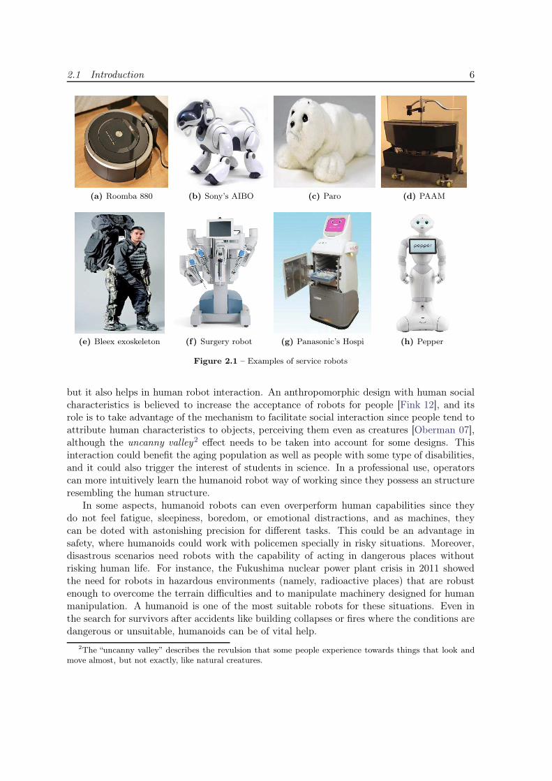
Most of the previously mentioned service robots are application dependent: they have beendesigned to satisfy specific needs. Some of them are shown in Fig. 2.1.
One of the main goals of service robotics is to make robots able to work and coexistside by side with humans in order to assist them. However, typical human environments arenot robot-friendly; that is, they are structured for people and not for robots. For instance,human environments present doors with a great heterogeneity, various forms of windows orglasses, obstacles and furniture almost everywhere, floors made of multiple materials andnot necessarily homogeneous, stairs and elevators to move from one floor to another, etc.[Soroka 12]. Hence, for robots to naturally interact with people, they must overcome all thesedifficulties with some degree of autonomy. Therefore, one of the biggest challenges of servicerobotics is to build general purpose robots that can succeed in all the areas where humanbeings can. Equivalently, the challenge is to build robots that act and behave as humans.
2.1.2 Why Humanoid Robots?
Perhaps the most natural response to the generic needs of service robotics is the developmentof robots with a human-like structure. This structure would allow them to perform well inhuman environments: they would be able to navigate anywhere inside a house, to go up anddown by the stairs, to walk on the street, to use human tools and machines, or to assist peoplein their daily life. But not only does anthropomorphism provide advantages for locomotion,
1ISO 8373:2012 Robots and robotic devices - Vocabulary
2.1 Introduction 6
(a) Roomba 880 (b) Sony’s AIBO (c) Paro (d) PAAM
(e) Bleex exoskeleton (f) Surgery robot (g) Panasonic’s Hospi (h) Pepper
Figure 2.1 – Examples of service robots
but it also helps in human robot interaction. An anthropomorphic design with human socialcharacteristics is believed to increase the acceptance of robots for people [Fink 12], and itsrole is to take advantage of the mechanism to facilitate social interaction since people tend toattribute human characteristics to objects, perceiving them even as creatures [Oberman 07],although the uncanny valley2 effect needs to be taken into account for some designs. Thisinteraction could benefit the aging population as well as people with some type of disabilities,and it could also trigger the interest of students in science. In a professional use, operatorscan more intuitively learn the humanoid robot way of working since they possess an structureresembling the human structure.
In some aspects, humanoid robots can even overperform human capabilities since theydo not feel fatigue, sleepiness, boredom, or emotional distractions, and as machines, theycan be doted with astonishing precision for different tasks. This could be an advantage insafety, where humanoids could work with policemen specially in risky situations. Moreover,disastrous scenarios need robots with the capability of acting in dangerous places withoutrisking human life. For instance, the Fukushima nuclear power plant crisis in 2011 showedthe need for robots in hazardous environments (namely, radioactive places) that are robustenough to overcome the terrain difficulties and to manipulate machinery designed for humanmanipulation. A humanoid is one of the most suitable robots for these situations. Even inthe search for survivors after accidents like building collapses or fires where the conditions aredangerous or unsuitable, humanoids can be of vital help.
2The “uncanny valley” describes the revulsion that some people experience towards things that look andmove almost, but not exactly, like natural creatures.
2.1 Introduction 7
In general, humanoid robots emerge like a panacea for service robotics. But althoughthe potential advantages greatly surpass the current capabilities, they provide a rationale toincrease the research in humanoid robotics and their applications.
2.1.3 History of Humanoid Robots
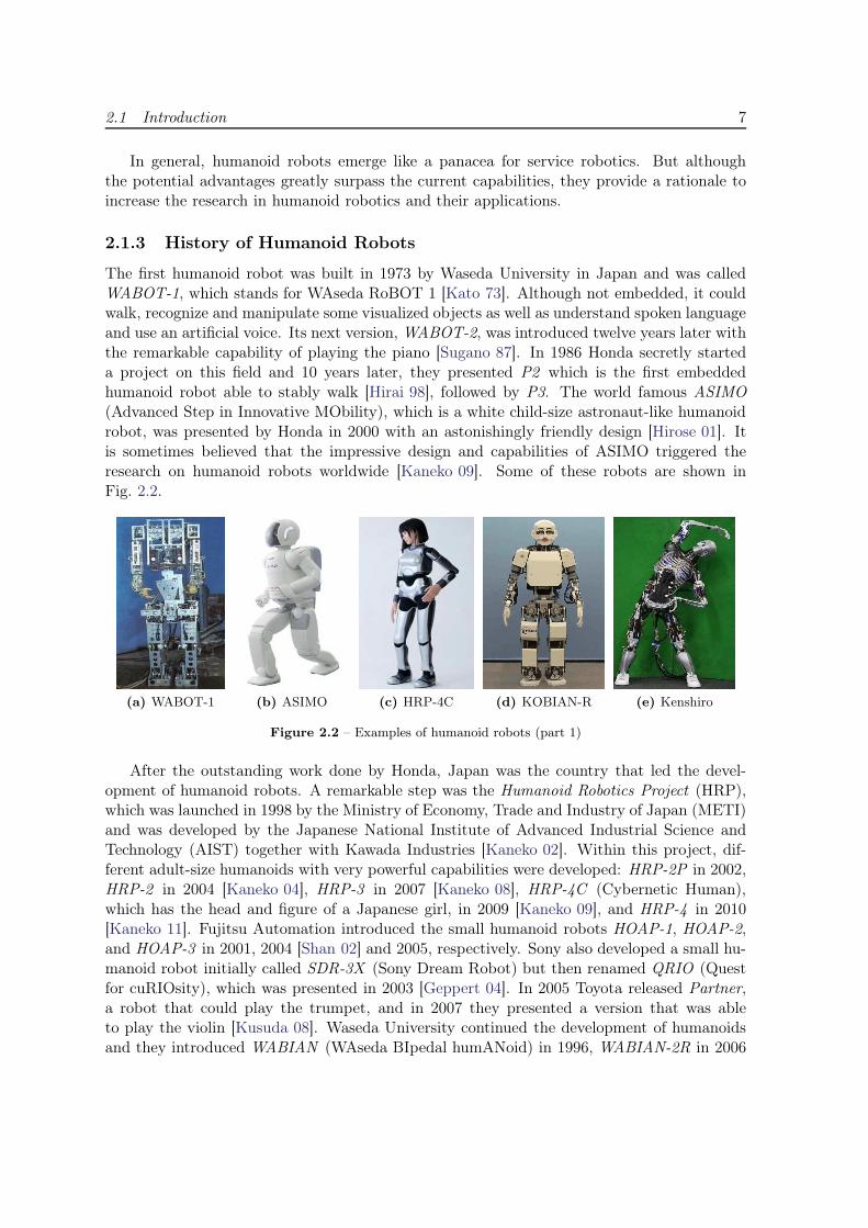
The first humanoid robot was built in 1973 by Waseda University in Japan and was calledWABOT-1, which stands for WAseda RoBOT 1 [Kato 73]. Although not embedded, it couldwalk, recognize and manipulate some visualized objects as well as understand spoken languageand use an artificial voice. Its next version, WABOT-2, was introduced twelve years later withthe remarkable capability of playing the piano [Sugano 87]. In 1986 Honda secretly starteda project on this field and 10 years later, they presented P2 which is the first embeddedhumanoid robot able to stably walk [Hirai 98], followed by P3. The world famous ASIMO(Advanced Step in Innovative MObility), which is a white child-size astronaut-like humanoidrobot, was presented by Honda in 2000 with an astonishingly friendly design [Hirose 01]. Itis sometimes believed that the impressive design and capabilities of ASIMO triggered theresearch on humanoid robots worldwide [Kaneko 09]. Some of these robots are shown inFig. 2.2.
(a) WABOT-1 (b) ASIMO (c) HRP-4C (d) KOBIAN-R (e) Kenshiro
Figure 2.2 – Examples of humanoid robots (part 1)
After the outstanding work done by Honda, Japan was the country that led the devel-opment of humanoid robots. A remarkable step was the Humanoid Robotics Project (HRP),which was launched in 1998 by the Ministry of Economy, Trade and Industry of Japan (METI)and was developed by the Japanese National Institute of Advanced Industrial Science andTechnology (AIST) together with Kawada Industries [Kaneko 02]. Within this project, dif-ferent adult-size humanoids with very powerful capabilities were developed: HRP-2P in 2002,HRP-2 in 2004 [Kaneko 04], HRP-3 in 2007 [Kaneko 08], HRP-4C (Cybernetic Human),which has the head and figure of a Japanese girl, in 2009 [Kaneko 09], and HRP-4 in 2010[Kaneko 11]. Fujitsu Automation introduced the small humanoid robots HOAP-1, HOAP-2,and HOAP-3 in 2001, 2004 [Shan 02] and 2005, respectively. Sony also developed a small hu-manoid robot initially called SDR-3X (Sony Dream Robot) but then renamed QRIO (Questfor cuRIOsity), which was presented in 2003 [Geppert 04]. In 2005 Toyota released Partner,a robot that could play the trumpet, and in 2007 they presented a version that was ableto play the violin [Kusuda 08]. Waseda University continued the development of humanoidsand they introduced WABIAN (WAseda BIpedal humANoid) in 1996, WABIAN-2R in 2006
2.1 Introduction 8
[Ogura 06], and the emotion expression robot KOBIAN-R in 2008 [Endo 08], which is ableto show different facial expressions. The University of Tokyo also developed a series of hu-manoid robots: H5, H6 in 2000, and H7 in 2006 [Nishiwaki 07], as well as musculo-skeletalrobots as Kenta, a tendon-driven robot, in 2003 [Inaba 03], Kotaro in 2006 [Mizuuchi 06], itsnew version Kojiro in 2007 [Mizuuchi 07], and more recently, in 2012, the impressive Ken-shiro [Nakanishi 12]. In 2013 the former Japanese Schaft Inc presented their last version ofthe Schaft robot, based on the HRP-2 series, which is currently one of the most powerfulhumanoid robots.
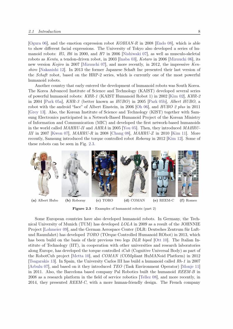
Another country that early entered the development of humanoid robots was South Korea.The Korea Advanced Institute of Science and Technology (KAIST) developed several seriesof powerful humanoid robots: KHR-1 (KAIST Humanoid Robot 1) in 2002 [Kim 02], KHR-2in 2004 [Park 05a], KHR-3 (better known as HUBO) in 2005 [Park 05b], Albert HUBO, arobot with the android “face” of Albert Einstein, in 2006 [Oh 06], and HUBO 2 plus in 2011[Grey 13]. Also, the Korean Institute of Science and Technology (KIST) together with Sam-sung Electronics participated in a Network-Based Humanoid Project of the Korean Ministryof Information and Communication (MIC) and developed the first network-based humanoidsin the world called MAHRU-II and AHRA in 2005 [You 05]. Then, they introduced MAHRU-III in 2007 [Kwon 07], MAHRU-R in 2008 [Chang 08], MAHRU-Z in 2010 [Kim 11]. Morerecently, Samsung introduced the torque controlled robot Roboray in 2012 [Kim 12]. Some ofthese robots can be seen in Fig. 2.3.
(a) Albert Hubo (b) Roboray (c) TORO (d) COMAN (e) REEM-C (f) Romeo
Figure 2.3 – Examples of humanoid robots (part 2)
Some European countries have also developed humanoid robots. In Germany, the Tech-nical University of Munich (TUM) has developed LOLA in 2009 as a result of the JOHNNIEProject [Lohmeier 09], and the German Aerospace Center (DLR: Deutsches Zentrum für Luft-und Raumfahrt) has developed TORO (TOrque Controlled Humanoid RObot) in 2013, whichhas been build on the basis of their previous two legs DLR biped [Ott 10]. The Italian In-stitute of Technology (IIT), in cooperation with other universities and research laboratoriesalong Europe, has developed the torque controlled iCub (Cognitive Universal Body) as part ofthe RobotCub project [Metta 10], and COMAN (COMpliant HuMANoid Platform) in 2012[Tsagarakis 13]. In Spain, the University Carlos III has build a humanoid called Rh-1 in 2007[Arbulu 07], and based on it they introduced TEO (Task Environment Operator) [Monje 11]in 2011. Also, the Barcelona based company Pal Robotics built the humanoid REEM-B in2008 as a research platform in the field of service robotics [Tellez 08], and more recently, in2014, they presented REEM-C, with a more human-friendly design. The French company
2.1 Introduction 9
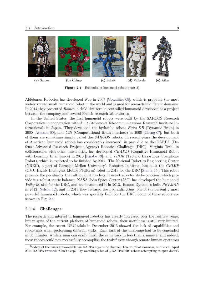
(a) Sarcos (b) Chimp (c) Schaft (d) Valkyrie (e) Atlas
Figure 2.4 – Examples of humanoid robots (part 3)
Aldebaran Robotics has developed Nao in 2007 [Gouaillier 09], which is probably the mostwidely spread small humanoid robot in the world and is used for research in different domains.In 2014 they presented Romeo, a child-size torque-controlled humanoid developed as a projectbetween the company and several French research laboratories.
In the United States, the first humanoid robots were built by the SARCOS ResearchCorporation in cooperation with ATR (Advanced Telecommunications Research Institute In-ternational) in Japan. They developed the hydraulic robots Erato DB (Dynamic Brain) in2000 [Atkeson 00], and CBi (Computational Brain interface) in 2006 [Cheng 07], but bothof them are sometimes simply called the SARCOS robots. In recent years the developmentof American humanoid robots has considerably increased, in part due to the DARPA (De-fense Advanced Research Projects Agency) Robotics Challenge (DRC). Virginia Tech, incollaboration with other universities, has developed CHARLI (Cognitive Humanoid Robotwith Learning Intelligence) in 2010 [Knabe 13], and THOR (Tactical Hazardous OperationsRobot), which is expected to be finished by 2014. The National Robotics Engineering Center(NREC), a part of Carnegie Mellon University’s Robotics Institute, has built the CHIMP(CMU Highly Intelligent Mobile Platform) robot in 2013 for the DRC [Stentz 15]. This robotpresents the peculiarity that although it has legs, it uses tracks for its locomotion, which pro-vide it a robust static balance. NASA John Space Center (JSC) has developed the humanoidValkyrie, also for the DRC, and has introduced it in 2013. Boston Dynamics built PETMANin 2012 [Nelson 12], and in 2013 they released the hydraulic Atlas, one of the currently mostpowerful humanoid robots, which was specially built for the DRC. Some of these robots areshown in Fig. 2.4.
2.1.4 Challenges
The research and interest in humanoid robotics has greatly increased over the last few years,but in spite of the current plethora of humanoid robots, their usefulness is still very limited.For example, the recent DRC trials in December 2013 showed the lack of capabilities androbustness when performing different tasks. Each task of this challenge had to be concludedin 30 minutes, while a man can easily finish the same task in less than a minute; and indeed,most robots could not successfully accomplish the tasks3 even though remote human operators
3Videos of the trials are available via DARPA’s youtube channel. Due to robot slowness, on the 7th April2014 DARPA tweeted: “Can’t sleep? Try watching 9 hrs of #DARPADRC robots attempting to open doors”.
2.1 Introduction 10
could control them. Moreover, all the walking humanoids fell down at least once while tryingto perform the task. This clearly shows that humanoid robotics is not a mature technologyyet, and there are still many control problems to overcome.
One of the biggest challenges involves the coordination and development of whole bodymotion, since humanoids are highly redundant typically with 30 to 40 degrees of freedom.During their motion, they usually have to interact with some objects; thus, manipulationbecomes an important part of the challenge. Also, humanoid robots are underactuated systemswhose position and orientation in the environment cannot be directly controlled but are theresult of the interaction with the environment and the proper joints motion [Wieber 06a].Moreover, this non-fixed interaction leads to a major concern: the robot must not fall downwhile performing a task. Thus, balance is of vital importance for humanoid robots, andthe control of the Zero Moment Point (ZMP) [Vukobratovic 69], or the Capture Point (CP)[Pratt 06b] have been proposed, although their integration within complex control frameworksis not straight forward.
The reduction of the computational cost to process the sensors information and to generateuseful movements for the robot is also currently a challenge. New, and more powerful artificialintelligence, computer vision, data fusion and navigation algorithms typically take time tocompute on very powerful machines. Furthermore, their usage within control frameworksthat use some model of the robot subject to physical and operational constraints to generatemotion trajectories presents the need for highly performant machines. In fact the achievementof real-time usually comprises a trade-off between accuracy and efficiency. And not onlyis the software level a challenge but also the hardware level: perception sensors such aspowerful vision systems, tactile mechanisms, as well as powerful actuators constantly need tobe improved [Durán 12]. All these problems are still to be overcome for humanoid robots tobehave as useful service robots able to help people in their daily life.
2.1.5 Applications of Humanoid Robots
Humanoid robots are virtually suitable for any environment where humans can work. Theycan become the universal worker for any manufacturing process since they can do repetitiveand even “intelligent” tasks without needing a special design. The generic design can evenmake the mass production of humanoids possible drastically reducing their cost. Works in-volving maintenance tasks of industrial plants, security services of homes and offices, humancare, and cooperative works can be possible. Teleoperation is also an important applicationprovided that the human structure makes their operation more natural for operators. Also,telepresence [Lee 12] can be carried out by humanoids.
Not only can humanoid robots work where humans can, but they can also work wherehumans cannot. In fact it is promising to use humanoids in tasks where human lives canbe at risk due to the environment or the task itself. Particularly a humanoid fire-fighter orrescuer is appealing for cases of natural disasters, fires, buildings collapse, general security orhazardous environments (like radioactive places). Space missions are another important areadue to the inherent dangerousness that space poses to astronauts or the complete currentinability to send a human to remote places. There is a need for a human complement orreplace and projects like NASA Robonaut [Ambrose 04] or DLR Justin [Wimbock 07] arealready addressing this problem. Military suits can also be tested without risking the life ofpeople [Nelson 12].

2.2 Approaches in the Control of Humanoid Robots 11
Another potentially big domain is household. Humanoids can one day become the mostused servant at home. Some projects explicitly address this problem like the Armar robot[Asfour 06], Twendy-One, or HERB [Asfour 06]. Humanoids can also be used for entertain-ment in robot competitions like FIRA (Federation of International Robot-soccer Association)and the RoboCup, whose initiative is that by 2050 a team of humanoid soccer players shallwin the soccer game, complying with the official FIFA rules, against the winner of the mostrecent World Cup [Kitano 98]. Also they can be used in biomechanics to have a deeper under-standing of how humans work and even think. In fact, humanoids can be used as platformsto test and develop cognition and artificial intelligence methods and some projects are alsodevoted to this field [Metta 10].
2.2 Approaches in the Control of Humanoid Robots
The control of a robot consists in defining a law that allows the generation of feasible motionwithin the limits of the mechanism such that a desired objective is achieved. As stated inSection 2.1.4, the control of humanoid robots poses particular challenges due to the redun-dancy, underactuation, the necessity to keep balance at every instant of time, and additionalconstraints to make motion human-like. Different methods can be used to make a robot movedepending on the application, the complexity of the task, and even the specific nature ofthe robot. The main control methods currently used for humanoid robots are the following:motion planning, inverse kinematics control, inverse dynamics control, and optimal control.This section discusses the state of the art in these approaches.
2.2.1 Motion Planning
Motion planning consists in automatically finding a feasible path from an initial configurationto a given goal satisfying certain constraints. In robotics, for instance, it can compute apath that moves the hand from its current pose to a desired one avoiding collision with someobstacles in the environment. For many purposes, it can be of great interest to determine thepath minimizing a convenient criterion. Currently, there are many applications in vehicles,robots, digital characters, molecules, design verification, amongst others.
Basic Concepts
Although the research in motion planning can be traced back to the late 60’s, most of theproblems formalization started in the 80’s thanks to the combined and growing research inartificial intelligence, computer science and mathematics. Currently, the main approachescan be found in books such as [Latombe 91, Choset 05, LaValle 06]. An important concept inmotion planning is the Configuration Space (CS), which is the set of all the possible config-urations that a mechanism can attain. This fundamental concept, borrowed from mechanicsand introduced by [LozanoPerez 83], can be used with several tools from geometry, topologyand algebra, and has provided the theoretical basis for motion planning.
For a robot with n independent degrees of freedom (DoF), the CS is an n-dimensionalmanifold M that contains all the configurations q ∈ M of the robot. The importance of theCS is that it changes the problem of moving a body in SE(3) to moving a point in CS. Twoparticular subspaces of CS are of interest:
2.2 Approaches in the Control of Humanoid Robots 12
• Obstacle Configuration Space (CSobst). It is formed by the robot configurations thatgenerate self-collisions or collisions with some object in the environment. The space isrepresented as CSobst ⊂ CS.
• Free Configuration Space (CSfree). It is the space where the robot can freely move andis the complement of the obstacle space: CSfree = CS − CSobst.
Using these spaces, the problem of motion planning can be stated as finding the continuouspath p(t) from a start configuration p(0) = q0 to a goal configuration p(1) = qf avoidingcollisions; that is, p : [0, 1] → CSfree, where t defines some parameterization.
Generic methods
The solution to the motion planning problem can be obtained using some classical methodswhich can be classified as: deterministic algorithms, sampling-based algorithms, and pathoptimization.
a) Deterministic algorithms. These algorithms, developed since the past 30 years, alwayscompute the same valid path p(t). Methods such as cellular decomposition, Voronoi dia-grams, visibility graphs and Canny’s algorithm rely on the construction of an explicit andexact representation of CSobst to build a graph, or roadmap, that represents the connectivityof CSfree [Goodman 04, Canny 88, Indyk 04]. Although these methods are complete, theybecome very computationally expensive in high-dimensional configuration spaces, even whenthe dimension of CS rises above 4. Other deterministic approaches use artificial attractivepotentials on the goals and repulsive potentials on the obstacles and the start configurationsto guide the search towards the goal avoiding the obstacles [Khatib 86]. However, the localityof this type of planners can lead to a solution that does not achieve the goal, for instance, ina maze environment.
b) Sampling-based algorithms. These methods, developed over the last 20 years, approx-imate the connectivity of CSfree by randomly sampling configurations from CS and reject-ing the configurations that produce collisions through Boolean collision detection techniques[Hudson 97, Gottschalk 96, Hsu 97]. The main examples are Probabilistic Roadmaps (PRM )[Kavraki 96], and Rapidly-exploring Random Trees (RRT ) [Kuffner 00]. In particular, theRRT algorithm uses the Voronoi bias to explore CSfree and grow a random tree. Each it-eration attempts to extend the tree by adding new vertices in the direction of a randomlyselected configuration. Trees can be grown from the initial and goal configurations, which issometimes referred to as Bi-directional RRT (BiRRT), making the algorithm more efficient[Kuffner 00]. Variations that asymptotically converge towards the global minimum solutionpath have been proposed as PRM* and RTT* [Karaman 11], for generic cases, and Kino-dynamic RRT* for systems with controllable linear dynamics [Webb 13]. RRT’s have alsobeen extended in the state space to LQR-Trees [Tedrake 10], which use a dynamic cost-to-godistance metric, and LQR-RRT* [Perez 12], which uses a linearization of the system to derivea coherent extension method. Stochastic-optimization for determining a new potential statebased on transition tests has been called the T-RRT (Transition-based RRT) [Jaillet 08]. Ingeneral, the advantages of these methods are their probabilistic completeness and their abilityto deal with very high-dimensional configuration spaces.
c) Path optimization. The goal of these methods is to optimize the trajectory startingwith a valid collision free path and trying to shorten it while ensuring that the path is still
2.2 Approaches in the Control of Humanoid Robots 13
valid. For example, greedy optimization tries to directly connect the start configuration tothe closest goal configuration node that generates a collision free path; then, it continues withthe next nodes in the path until reaching the goal. Another example is random optimizationwhich tries to ignore some random nodes keeping the rest.
Motion Planning in Humanoid Robotics
Classical motion planning methods determine collision-free trajectories involving only geo-metrical considerations. However, the control of polyarticulated systems needs the synthesisof models that describe the effects of joint variations on the whole robot configuration. Forinstance, moving an arm with only RRT’s considering environmental and self-collisions caneffectively achieve the goal configuration, but the arm risks to make very unnecessary, unnat-ural and inefficient movements. Underactuated robots present the additional problem thatthe planning algorithm might generate paths that do not preserve the balance of the robotor the motion might not be physically plausible. To overcome these problems within theseframeworks, trajectories are generated using methods of inverse kinematics, inverse dynamicsor optimal control and additional constraints are added to satisfy conditions like multiplecontacts or the dynamic balance of the system. For instance, motion primitives that havebeen predefined by a human expert based on prior knowledge can be used to guide the planner[Zhang 14].
For humanoid walking, footsteps planning can be achieved using deterministic approacheswith dynamic adjustment of the footstep transition model [Chestnutt 05] considering thesmoothness of the trajectories for posture transitions [Ayaz 07]. But these approaches donot guarantee the completeness of the solutions and probabilistically complete methods havebeen proposed to solve this problem. For instance, RRT’s can be adapted to explore thediscrete footstep space [Xia 09, Perrin 12], and anytime search-based planners can be usedto generate paths that are goal-directed guaranteeing to stay within bounded limits from theoptimal solution [Hornung 13]. Also, features of the environment can be used to guide towardsthe solution; for instance, multi-contact planning can be achieved using a multiple-contact-point stance planner that looks for authorized contact surfaces to help the robot reach itsgoal [Bouyarmane 12a, Escande 13]. Other approaches divide the high-dimensional probleminto smaller problems and solve them successively [Zhang 09]. An example is presented in[Yoshida 08], where a 36 degree of freedom robot is reduced to a 3 degree of freedom boundingbox and a PRM is applied for the path planning problem of the box.
During the last few years, planning on constraint submanifolds of CS has been the focusof many researches. For example, manifolds can be defined by contact limb positions andstatic balance constraints, and the plan can be done on a union of submanifolds. In this way,statically balanced locomotion for hexapods and humanoid robots on uneven terrain can beobtained [Bretl 06, Hauser 10]. Another method proposed the planning algorithm CBiRRT(Constrained Bidirectional RRT) together with some Jacobian-based methods to consider end-effector pose constraints in the plan and generate humanoid motion [Berenson 11]. Also, RRTcan be adapted within a random diffusion framework to work according to some constraintand generate statically stable configurations [Dalibard 13]. More recent methods combinepath planning with optimal control to generate motion for humanoid robots in a clutteredenvironment [ElKhoury 13].
2.2 Approaches in the Control of Humanoid Robots 14
2.2.2 Inverse Kinematics (IK)
Kinematics, in general, is the study of the position, velocity and acceleration of a mechanicalsystem without considering either the forces (or torques) that generate the motion or thedynamic properties, such as mass or inertia, of the bodies composing the system.
Basic Concepts
The joint space, also called the configuration space, of a robot with n DoF is the n-dimensionalmanifold Q containing all the possible values that the joint variables q can take. For roboticmanipulators, the pose of a single element called the end-effector is typically of interest.However, for more generic robots such as humanoids, this is generalized to the operationalpoints [Khatib 87], which can represent any part of the robot whose pose is of interest. Thevelocity of an operational point x can be represented by the twist [Murray 94] or spatial velocity[Featherstone 08] ξ that comprises both the linear and angular velocities; alternatively, it canbe given by the variation of its representation x. In robotics there exist four sub-domainsrelated to kinematics.
• Forward kinematics (also called forward geometry4). It consists in finding the posex ∈ SE(3) of an operational point given a certain joint angle configuration q ∈ Q, andis described by the map f : Q → SE(3) such that x = f(q).
• Inverse kinematics (also called inverse geometry4). It aims at finding the joint config-uration q ∈ Q that achieves a given pose x ∈ SE(3) for a certain operational point. Insome specific cases, this can be represented by the inverse map f−1 : SE(3) → Q suchthat q = f−1(x), but in general f−1(x) is not unique and can even be undefined.
• Forward differential kinematics (also called forward instantaneous kinematics or simplyforward kinematics4). It consists in finding the operational-point twist ξ ∈ se(3) thatis produced due to joint variations q ∈ Tq(Q), which is expressed as ξ = Jo(q)q, whereJo : Tq(Q) → se(3) is the tangent application called the basic [Khatib 87] or geometricJacobian [Spong 06], and Tq(Q) is the tangent space to Q at q. Alternatively, it canbe formulated as finding the first order variations x that are produced by q, expressedas x = ∂x
∂qq. In this case, J(q) = ∂x
∂qis a differential map called the analytic or task
Jacobian [Spong 06] or simply the Jacobian [Khatib 87].
• Inverse differential kinematics (also called inverse instantaneous kinematics or simplyinverse kinematics4). It is the problem of finding the joint variations that produce agiven variation of the end effector (Section 3.2.2). It can be used to iteratively solve theinverse kinematics problem.
In general, the control objective is defined by a reference point or a reference trajectory inSE(3), and the control problem consists in determining the appropriate evolution of the jointconfiguration q(t) that achieves the objective. Consider the task i with mi DoF. An n-DoFrobot is said to be kinematically redundant with respect to task i if n > mi, and n − mi
4The Greek root “kinesis” refers to movement or motion; therefore the term geometry is more accuratethan kinematics when the map is between static spaces. Similarly, when velocities are implied, kinematics ismore accurate than differential kinematics.
2.2 Approaches in the Control of Humanoid Robots 15
is known as the degree of redundancy with respect to task i [Nakamura 90]. If there are ksimultaneous tasks, each of them with mi DoF, the system is still kinematically redundant ifn >
∑ki=1mi.
Classical Kinematic Methods
Forward kinematics is traditionally represented using the classical Denavit-Hartenberg (DH)parameters [Denavit 55], or the modified DH parameters introduced in [Craig 89], but al-though very popular for serial manipulators, they might lead to ambiguities for closed or treechains [Khalil 04] and can even be not suitable for robot calibration [Everett 87]. Alternativemethods have been proposed: the Khalil-Kleinfinger notations that are suitable for closed-loop robots [Khalil 86], the Hayati-Roberts coordinates that avoid coordinate singularities forparallel systems [Hayati 85, Roberts 88], the products of exponentials (PoE) [Park 94], screwtheory-based kinematic modeling [Tsai 99], or even ad-hoc methods for specific cases such asfor humanoid robots [Kajita 05].
For simple kinematic chains, the IK problem can be analytically solved and closed equa-tions can be obtained through two classical types of approaches: (i) algebraic approaches, suchas inverse transforms [Paul 81] or dialytic eliminations to derive polynomials [Raghavan 93];and (ii) geometric approaches like joint decoupling when the last three joint axes inter-sect [Peiper 68] or the so-called Paden-Kahan sub-problems which are based on the PoE[Paden 86, Kahan 83]. However, as the complexity of the chain increases, the complexity ofthe analytical solution also increases due to the strong non-linear terms. For more compli-cated chains, analytical solutions become tedious or even ill-posed due to the redundancy ofthe system.
Kinematic Control of Redundant Robots
Even though kinematic redundancy offers more dexterity and versatility to the robot, likejoint range availability, singularity avoidance, obstacle avoidance, compliant motion or energyconsumption minimization, it increases the complexity of inverse kinematics [Siciliano 91].For a given task, there is more than one solution in the joint space, and closed form solutionsare in general not possible. Moreover, solutions that satisfy both the main task and othercomplementary tasks as closely as possible are usually desired. For instance, a redundantmanipulator has typically to achieve the goal pose avoiding collisions with objects in theenvironment. In these cases, numerical methods are preferred and have shown to offer goodresults.
Numerical methods treat the IK problem as an optimization problem with, in some cases,additional constraints. There are two main approaches for solving IK through optimization:(i) Global methods, which find an optimal path for the entire trajectory but have a highcomputational cost [Baillieul 90]; and (ii) Local methods, which are used in real time andonly compute an optimal change ∆q for a small change ∆x, integrating ∆q to generate thejoint space trajectory q(t). A well-known local method is the Resolved Motion Rate Control[Whitney 69] which finds the change of q as a solution to the problem x = J(q)q using theinverse J−1, if J is invertible, or a suitable pseudo-inverse J+. In order to avoid problemswith singular configurations, the damped pseudo-inverse can be used instead [Nakamura 86,Wampler 86]. A more generic solution arbitrarily adds a projection onto the nullspace of
2.2 Approaches in the Control of Humanoid Robots 16
J since doing so does not modify the desired x but supplies some freedom for other tasks[Liegeois 77]. When there are two or more tasks to be satisfied at the same time, somecompromises have to be taken into account. To this end, there are two main methods:
• Task space augmentation. It is a weighting approach that extends the dimension ofthe original task space by imposing constraints to the joint variables [Sciavicco 87].Problems occur when tasks conflict with each other because they implicitly have thesame priority. In these cases, weights are assigned to each task and a compromiseamong them is found, although no task is completely satisfied. To choose a constrainttask that avoids conflicts with other tasks, an approach called the Extended Jacobianmethod (EJM) zeroes the projection of the cost function gradient in the null space ofthe Jacobian [Baillieul 85].
• Task prioritization. It consists in generating a set of prioritized tasks where the lowerpriority task produces a self-motion that does not interfere with the higher priority taskleading to a multiple priority-order resolution method [Nakamura 87]. The approachfinds a joint velocity q such that every task xi is satisfied unless it conflicts with ahigher-priority task xj , (j < i), in which case its error is minimized. An algorithmicsolution was proposed in [Siciliano 91] and improvements in the algorithmic computationof the null-space projector were introduced in [Baerlocher 98].
Kinematic Control of Humanoid Robots
From a kinematic point of view, humanoid robots present a tree-like structure that includesmultiple connected chains, and a high number of DoF. As a consequence, the kinematicstructure is often redundant with respect to most tasks, in which case the robot is said to beunder-constrained. Therefore, methods developed for generic redundant robots are usuallyapplied in humanoid robotics with some adaptations or additions. Due to the complexityof the kinematic configuration, closed-form solutions for the IK problem are usually verycomplex, but recently some classical methods have been used and modified, to obtain closedequations for specific humanoid robots which are treated as a composition of several kinematicchains [Ali 10, Nunez 12]. However, methods based on instantaneous IK, which compute anincrement in q, are usually preferred. This linearization of the problem offers an infinitenumber of feasible solutions for humanoid robots: there exist different joint updates thatachieve the same task. This leads to the possibility of performing different tasks at the sametime, and the IK control must be capable of properly handling them.
Some works have proposed the usage of a weighting approach, such as [Tevatia 00] that usesa simplified EJM augmenting the task space, or [Salini 09] where a continuous variation of theweight values is associated to each task relatively to its importance. Due to the nature of theseschemes, problems arise when there are conflicting tasks since in those cases none of the taskscan be fully satisfied. Methods based on task-prioritization solve these problems and havebecome the preferred techniques in IK control. They can even be considered as the current“state of the art” in humanoid robotics control due to their relatively low computationalcost, their straightforward implementation, and the maturity of the approach. Several workswith different humanoid platforms use this methodology to solve the redundant IK problemat the velocity level using only equality constraints [Gienger 05, Yoshida 06, Mansard 07,Neo 07, Galdeano 14]. For imposing inequality constraints to the control framework at any
2.2 Approaches in the Control of Humanoid Robots 17
hierarchical level, a sequence of optimal resolutions for each priority level has been proposed in[Kanoun 09], a more efficient computation based on orthogonal decompositions can be foundin [Escande 14] and a smooth interchange between priority of consecutive prioritized tasks isintroduced in [Jarquin 13].
2.2.3 Inverse Dynamics
Dynamics is the study of the relation between the robot motion and the generalized forcesthat act on the robot generating that motion. This relation considers parameters such aslengths, masses and inertia of the elements composing the robot.
Basic Concepts and Computation
In the dynamic model, the motion is represented through joint variables acceleration q, oroperational points acceleration x. For rotational joints, the generalized forces are equivalentto the joint torques, and for prismatic joints they are the joint forces. There are two mainproblems in dynamics:
• Forward Dynamics. It expresses the motion of the robot as a function of the generalizedforces applied to it.
• Inverse Dynamics. It expresses the generalized forces acting on a robot as a function ofthe robot motion.
There exist two main formulations to compute the robot dynamic model: the Lagrange ap-proach, and the Newton-Euler approach. The Lagrange approach was the first one used inthe robotics community [Uicker 67, Kahn 71, Bejczy 74]. Its main advantage is the clearseparation of each component of the model; but in general, it is computationally expensive,although an efficient formulation was presented in [Hollerbach 80]. The Newton-Euler ap-proach, proposed in [Orin 79], does not provide a clear separation of the terms but due to itsrecursivity a lower computation time can be obtained. Thus, it is the preferred implementa-tion for computer calculations. The most used algorithms for this approach can be found in[Featherstone 00, Featherstone 08], for instance, the composite-rigid-body algorithm (CRBA),the articulated-body algorithm (ABA), the recursive Newton-Euler Algorithm (RNEA), andsome global analysis techniques. Although currently less used in robotics, the Hamiltonianapproach has also been applied to the analysis of robot dynamics [Spong 92] and numericalmethods for integrating Hamilton’s equations are becoming more efficient [Selig 07].
The term centroidal momentum has been recently proposed as the sum of the individuallink momenta expressed at the robot Center of Mass (CoM) [Orin 08], and the dynamicsexpressed at the CoM has been introduced as centroidal dynamics [Orin 13]. This is a partic-ularly important concept since the motion of humanoid robots typically involves large angularmomenta. The dynamic model of a robot can be expressed in two ways depending on thespaces that are used to describe the motion and the control input. The two approaches are:the joint space formulation, and the operational space (or task space) formulation. The jointspace formulation is the classical approach and uses the joint space acceleration to specify themotion, and the generalized forces acting on the actuated joints to describe the control. Theoperational space formulation [Khatib 87] represents the motion directly using the task spaceacceleration, which needs a reformulation of the forces as task space generalized forces.
2.2 Approaches in the Control of Humanoid Robots 18
Dynamic Control of Robotic Manipulators
The dynamic control of a robot consists in finding the proper generalized forces that haveto be applied to the joints in order to generate the desired trajectory for an operationalpoint. Classical methods for robotic manipulators include two main types of control: (i)Joint Space Control, which is based on the joint space formulation and includes methods suchas PD and PID controllers [Arimoto 83], inverse dynamics control (in this context usuallycalled computed torque [Markiewicz 73]), robust control in presence of parameter uncertainty[Lozano 92], Lyapunov-based control [Slotine 87], adaptive control [Dubowsky 79], adaptivecompensation of gravity [Tomei 91], amongst others; and (ii) Operational Space Control,based on the operational space formulation with methods such as inverse dynamics control[Caccavale 98] or PD control, amongst others [Nakanishi 08].
For redundant manipulators, one of the first approaches was the Extended OperationalSpace formulation that proposes the dynamic control of joint-space postures and adds nullspacevectors to the rows of the Jacobian [Park 01]. A similar approach of augmenting the Jaco-bian is used in [Harmeyer 04], and a projection of the dynamics onto a constrained consistentmanifold using the decomposition of the constraint Jacobian is proposed in [Aghili 05]. Basedon the resolved motion rate control in kinematics, the resolved acceleration control, whichrelates the task acceleration to the joint acceleration [Luh 80], was proposed for the fixedupper body of a humanoid robot but with the limitation that only kinematic constraints likecollision avoidance and joint limits can be used in the framework [Dariush 10].
Dynamic Control of Humanoid Robots
For a humanoid robot, classical dynamic control techniques are not sufficient since coordina-tion of the motion is required, environmental forces need to be considered, and balance hasto be kept at all moments. For the robot balance, a stability criterion such as keeping theCoM or the ZMP (Section 3.1.2) inside the support polygon must be enforced [Wieber 02].For planar surfaces the constraint on the ZMP implies a control of the contact forces. Thus,the interaction with the environment is always present since the feet are in contact with theground and additional contacts of other parts of the robot body might also be necessary.These contacts generate an effect on the joints generalized forces, which cannot be controlledusing only kinematic methods but with dynamic approaches. The dynamic control ensuresthe physical feasibility of the motion and allows for faster movements without losing balance.
The operational-space inverse-dynamics (OSID) is a more specific framework for control-ling the whole-body of humanoid robots considering contacts and a set of different constraints.The first approach, proposed in [Khatib 04b, Sentis 05], is based on a two stage mapping toobtain consistent contact forces and is equivalent to successive projections onto the nullspacesof the previous tasks. Therefore, new tasks can be added without dynamically interferingwith higher priority tasks. An approach based on orthogonal decompositions and projectionsto resolve over-actuation in double support, avoiding the inversion of the inertia matrix andgaining robustness against model uncertainty, was presented in [Mistry 10]. Although bothapproaches differ in their formulation, it has been shown that they are equivalent with respectto the minimization of different cost functions [Righetti 11b]. An improvement to this ap-proach consists in creating an optimal distribution of contact constraints by pushing groundreaction forces inside the frictional boundaries [Righetti 11a]. However, these methods onlydeal with equality dynamic constraints. Generic tasks or constraints specified as inequalities,
2.2 Approaches in the Control of Humanoid Robots 19
which are important to specify joint limits, collision avoidance, visual field tasks, amongstothers, cannot be taken into account in a straightforward way.
Other methods use the OSID within frameworks that involve some type of optimizationto find the local solution. The most popular approaches use Quadratic Programming (QP),which allows for the specification of both equality and inequality constraints. The lattertype of constraints is fundamental in humanoid robotics to directly model unilateral contacts,and it is also important to properly specify some particular tasks. A weighting scheme isused within a QP in [Collette 08] to control different objectives, but the approach is mainlyoriented towards robust balance. Another similar weighting approach is oriented towardsthe sequencing of dynamic tasks, computing the torque controls to satisfy the constraints[Salini 11]. The decoupling of the humanoid dynamics into holonomic and non-holonomic partbased on the Gauss principle [Wieber 06a] has been also exploited within a QP to producefeasible whole body motion in [Bouyarmane 12b]. An implementation for the lower part of atorque-controlled humanoid robot has been shown in [Herzog 13] using active set QP solvers.Also, OSID has been used within a prioritized scheme that allows the usage of for bothequalities and inequalities at any level of the hierarchy [Saab 13].
Although the previous approaches exploit the full robot dynamics, the angular momentumis not explicitly controlled within these frameworks. Nevertheless, it has been shown thatthe angular momentum is a natural and important part of human motion, specially whenperforming complex and fast movements [Popovic 04]. One of the first attempts to controlthis physical quantity for whole-body motion used a pseudo-inverse of the inertia matrix[Kajita 03b]. Other control schemes propose to control the angular momentum through thecontrol of the system’s centroidal momentum, such as [Hofmann 09] where the focus is on gatemovement, or [Moro 13] where the centroidal momentum is defined as an attractor withinthe framework. Also, a prioritization scheme based on a conic optimization to control thecentroidal angular momentum generating movements like kick and jump has been introducedin [Wensing 13].
Dynamic Control in Computer Graphics
In computer graphics, there has also been the need of using the dynamics of human-likecharacters to generate motion that satisfies dynamic constraints [Popovic 00]. For instance,retargeting motion to characters with different physics adds more realism to the animation[Gleicher 98]. B-splines are also used to retarget characters [Lee 99] but some physical limitsare not explicitly checked. Another approach adapts a given motion to a character keeping thecontact between the limbs and external objects [Shin 01]. More recent works have introducedQPs to generate physically consistent motion guiding humanoid avatars to achieve varioustasks through weights that establish the relative importance of each task [Abe 07]. Otherexamples of weighting schemes in this field include [Macchietto 09], where the focus is onbalance, and [DaSilva 08] where a Model Predictive Control (MPC) is used to track motions.An approach based on a novel prioritization algorithm, which uses a nested sequence of ob-jectives re-parameterized at each level of the hierarchy, has been proposed in [deLasa 10] withthe name of feature-based control. Motions like balancing, jumping or walking for a humanoidrobot-like character have been achieved using different tasks with this control method. Thisapproach has been later extended within an optimal control framework [Brown 13]. However,there exists a gap between physically plausible animations and real motion on the robot, and
2.2 Approaches in the Control of Humanoid Robots 20
the motion generated in computer animation does not guarantee a feasible direct reproduc-tion on a real humanoid. In reality, physical interactions between the feet and the groundsignificantly affect the whole body motion and errors in considering them can cause the robotto fall down making the generated motion completely unfeasible.
2.2.4 Optimal Control
Optimal control, also known in robotics as trajectory optimization or trajectory filtering, con-sists in finding a trajectory and its associated control law (policy) that satisfies some pre-defined optimality criterion. In general mathematical terms, it concerns the properties ofcontrol functions which, when inserted into a differential equation, give solutions that min-imize a cost or measure of performance. But it also concerns optimization problems withdynamic constraints which might be functional differential equations, difference equations,partial differential equations or equations with another form.
Introduction
It is often said that optimal control started more than 300 years ago [Sussmann 97], withthe solution to the brachystochrone problem by J. Bernoulli. But most formalization on thisfield began about 60 years ago with the introduction of the linear quadratic control problem[Wiener 49] as a minimization of a mean-square-error criterion with the form J = E{e2(t)},where e(t) is the error and E{x} represents the expected value of the random variable x. An-other major step was the introduction of Dynamic Programming (DP) [Bellman 56], whichreduces the search to a partial differential equation called the Hamilton-Jacobi equation, intro-duced to solve discrete-time optimal control problems. However, it is sometimes consideredthat optimal control was not completely formalized until the formulation of the maximumprinciple in [Pontryagin 62], which is strongly based on the Calculus of Variations. In fact,calculus of variations is considered as the roots for optimal control and presents the notablefeature of taking account of pathwise constraints on values of the control functions. Anotherremarkable formulation was the linear quadratic regulator (LQR) and the linear quadraticGaussian (LQG) in [Kalman 60] to design optimal feedback control laws.
In industry, a control methodology based on the solution of an optimal control problemat each controller update time over a time interval, known as the prediction horizon, evolvedwith the name of Model-based Predictive Control or simply Model Predictive Control (MPC)[Richalet 78]. It is sometimes also called receding horizon control, or preview control. Cur-rently, MPC constitutes one of the most powerful optimality methods for automatic control.It offers the possibility of specifying high-level task goals through simple cost functions, and itautomatically synthesizes all the details of the behavior and control law. Another advantageis that MPC avoids the need for extensive exploration by postponing the design of the policyuntil the last minute, finding controls only for the states that are currently visited. Thatis, it foresees the future states of the system to choose the best current state according tosome pre-established criteria. Other important method is Differential Dynamic Programming(DDP) [Jacobson 68] which is a local trajectory-based numerical scheme that provides an ef-ficient solver for direct implicit optimal control problems. A local-global hybrid method withconstant local controllers was introduced in [Atkeson 94], and it was complemented by theusage of second order local DDP models to make locally-linear controllers in [Atkeson 03].
2.2 Approaches in the Control of Humanoid Robots 21
Optimal Control of Humanoid Robots
In robotics, optimal control can be used to find the trajectories from an initial posture to afinal desired posture, specified as a whole or as a set of sub-objectives, satisfying certain con-straints. Very fast and powerful movements can be generated with optimal control, which cancomprehend the problems of inverse kinematics or inverse dynamics and can therefore pro-duce better movements. The problem with IK and OSID alone is their inability to properlyhandle the CoM accelerations, thus overrestricting the motion. A solution typically relies ona dedicated submodel, like a linearized inverted pendulum [Kajita 03a] to capture the futureof the system, but this ad-hoc resolution increases the control architecture complexity. Thus,using these schemes the future states of the system can be somehow predicted, but dedicatedsubmodels would need to be developed for each case. However, optimal control is the mostsuitable approach that allows to take into account all the constraints at the same time. Infact, optimal control can automatically generate the proper trajectory for the CoM in orderto achieve fast movements: it acts as a classical pattern generator used for walking schemes,but additionally incorporating whole-body motion. A serious challenge to optimization-basedapproaches in robotics is that the timescales of the dynamics are faster than in other appli-cations and need a faster response. Currently, the main problem is the computational time,due to the high number of DoF, that forbids its use in real-time applications.
An optimal control method of particular interest in humanoid robotics is MPC. Oneof the first uses of MPC in robotics was the so-called walking pattern generator (WPG)[Kajita 03a, Herdt 10] which previews the future states of the robot to generate a trajectoryfor the CoM which enables dynamic stability. In case of multi-task scenarios, a weighted sum ofthe task objectives can be applied choosing the weights proportionally to the task priority level[Dimitrov 11], but too low weights may lead to interferences between tasks and large weightscan introduce numerical conditioning problems. An alternative to weighting task errors isthe prioritized optimal control proposed in [DelPrete 14b], which ensures that the specifiedpriorities among the tasks are respected avoiding numerical conditioning issues. To speed upthe computation of dynamic derivatives, a physics simulator called MuJoCo was introduced[Todorov 12], and using MPC, it has allowed to synthesize humanoid behaviors such as gettingup from the ground and recovering from large disturbances [Tassa 12]. Other complex dynamicmotions examples obtained using optimal control are ball-kicking [Miossec 06], weight-lifting[Arisumi 08], and parkour movements [Dellin 12].
Optimal control methods have also proved to be very powerful tools to generate multi-ple non-coplanar contact motion, which increases the accessible space of humanoid robotsusing the environment to help them achieve the goal [Lengagne 13]. For robots in clut-tered environment, with many obstacles, some methods combine motion planning algorithmswith optimization. For instance, CHOMP (Covariant Hamiltonian Optimization for MotionPlanning) [Zucker 13], STOMP (Stochastic Trajectory Optimization for Motion Planning)[Kalakrishnan 11], and ITOMP (Incremental Trajectory Optimization for Real-Time Replan-ning in Dynamic Environments) have been recently introduced for robotic manipulators butcan be extended to humanoid robots considering additional constraints [Park 14]. CHOMPuses penalty terms to obtain an efficient optimal control solver which relies on a covariantgradient descent technique, and STOMP is a similar solver but relies on trajectory stochasticperturbations so that collision-free optimal trajectories can be found without computing func-tion Jacobians. Based on CHOMP, ITOMP provides a suboptimal solution if the optimization
2.3 Conclusion 22
task has not been solved within time constraints and updates the trajectory online.To include inequality constraints without sacrificing convergence or computational effort,
a generalization of DDP, called control-limited DDP, has been proposed and applied in simu-lation to a humanoid robot [Tassa 14]. Another variant of the DDP has been proposed withthe name of square-root DDP [Geoffroy 14] showing that IK can be seen as a particular caseof optimal control when there is no preview horizon. Similarly, OSID is a particular case whenno preview horizon is used. A guided policy search algorithm that uses trajectory optimiza-tion to direct policy learning and avoid poor local optima has been proposed in [Levine 13],where DDP generates guiding samples. This method has learned neural network controllersfor planar swimming, hopping, and walking, as well as simulated 3D humanoid running. UsingDP, walking behaviors robust to external disturbances and modeling errors have been gener-ated in [Whitman 13], where multiple-model variants and learning-based variants of DP areproposed. Another method uses the so called Body Retention Load Vector index to representthe physical constraints and achieve steep climbing [Noda 14]. For the animation of physics-based human-like characters, some impressive results have been shown in [AlBorno 13] whoseapproach optimizes a small set of simple goals applied to short space-time windows composedto express goals over an entire animation. The method synthesized motion with consider-able rotation components such as rolling motion [Brown 13], or more recently, walking, handwalking, breakdancing, flips, and crawling [AlBorno 14], which have never been previouslysynthesized by physics-based methods.
Optimal control has also been used to model human-like running as an offline control prob-lem solved by a direct multiple shooting method optimizing energy-related criteria [Schultz 10].There is also research on optimization-based motion generation for walking motions with-out the use of a WPG but with different objective functions such as the minimization oftorques, joint velocities or more complex combinations, and constraints such as the ZMP[Koch 12, ElKhoury 13]. Another area is inverse optimal control, which has been proposed asa means to determine, for a given dynamic process and an observed solution, the optimizationcriterion that has produced the solution. In particular, motion capture data of people hasbeen used to determine the principles of human locomotion and the path generation to giventarget positions and orientations [Mombaur 10]. It has also been used to learn the functionfor human running on flat ground, rough terrain and under lateral perturbation [Park 13].
The main drawback of optimal control is the curse of dimensionality, which is particularlyimportant for humanoid robots whose state space is so large that no control scheme canexplore all of it in advance and prepare suitable responses for every situation. It would bedesirable to obtain optimal control in real time; however, currently there is no approach thatcan achieve this: the solutions are very time consuming and generic solvers tend to get stuckinto local minima or they even return trivial solutions. The problem of finding the properformulation and resolution of optimal control is still an open issue in robotics.
2.3 Conclusion
Throughout recent years there has been a vast development of human-like robots, which arepotentially the best candidates for service robotics since they can move in human environmentsand perform tasks that humans do in their daily life. This development has led to maturetechnologies at the hardware level: very robust and powerful platforms can be found nowadays

2.3 Conclusion 23
in research centers. However, there currently exists a gap between what a humanoid platformis able to do and what it can really do. The main reason is the lack of suitable control systemsthat exploit all the potential and the advantages that such platforms offer. These systemshave to deal with aspects such as balance, redundancy, underactuation, motion coordination,environmental interaction amongst others, which make humanoid robot control a difficultproblem.
This chapter has presented the state of the art in control approaches for humanoid robots.Motion planning was among the first frameworks used to determine paths in the configurationspace and several improvements, some of which have been specially designed for humanoidrobots, have recently appeared. Methods based on inverse kinematics have been recalledfirst for redundant robots and then specifically for humanoid robots. In many ways, inversekinematics can be considered as the ’de facto’ state of the art in robot control since it isa well understood and used approach due to its simplicity and real-time capabilities. Then,inverse dynamics control, which is a step forward in control with respect to inverse kinematics,was recalled for robotic manipulators, humanoid robots and computer animations. Finally,optimal control approaches, which constitute the most promising automatic motion generationmethodologies, were briefly discussed.

Chapter 3
Inverse-Dynamics Whole Body Motion
Whole-body control of a humanoid robot is a challenging task due to the kinematic anddynamic complexity of the system. Humanoids are highly kinematically redundant robotswith a non-trivial tree-like structure as well as an unstable nature due to the vertical po-sition. At every moment, the robot must not only reproduce some task, but it should notfall while performing the task, keeping its dynamic balance. As described in the previoussection, several methods aiming at solving these problems have been recently proposed andthe research area is very active. The generic method proposed in this thesis is based on theinverse-dynamics model of the robot considering contact constraints and a set of tasks spec-ified with a given priority. The resolution for each task is posed as a minimization problem,subject to several constraints that ensure dynamic feasibility, and uses a hierarchical schemebased on hierarchized QPs. Since the motion is generated using several prioritized tasks, andthe dynamic model of the robot is taken into account, the term Dynamic Stack of Tasks (SoT)is sometimes used to refer to the framework. With respect to other operational-space inverse-dynamics (OSID) approaches, the advantages of the proposed method are the capability tohandle both equality and inequality constraints at any level of the hierarchy, the fast compu-tation time that allows it execution in real-time, and the direct feasibility of the generatedmotion, which does not need any further processing or validation before being executed onthe robot.
This chapter presents the foundations of the proposed methodology and is divided asfollows. First, the task-function formalism, which is the basic form in which the motionobjectives are specified, is recalled. Then, the dynamic model of the robot is presentedconsidering the underactuation of the system as well as the rigid contact constraints. Thecontrol scheme based on hierarchical quadratic programming is then treated in its initialformulation and also in the reduced form to speed up the computational time and achievereal-time performance. Finally, different types of tasks used throughout the thesis to generatedifferent kinds of motion are presented.
3.1 Dynamic Considerations for a Humanoid Robot 25
3.1 Dynamic Considerations for a Humanoid Robot
The dynamic model of the robot states the relation between the generalized control torquesτ and the generalized joint accelerations q. Unlike robotic manipulators, a humanoid robotis not attached to some part of the environment but presents a continuous interaction: thefeet of the robot are continuously touching the ground, and other parts of the robot suchas the hands, can also be in contact with the environment. Hence, the constraints imposedby the considered contact model must be satisfied for the motion to be feasible. Moreover,a humanoid robot is also an underactuated system, whose motion is possible due to theinteraction with the environment, and balance must be kept throughout all the motion. Thus,the representation of the robot must explicit this underactuation and some balance constraintsmust also be satisfied. The full dynamic model includes both the contact constraints and theunderactuation and is presented at the end of this section.
3.1.1 Rigid Contact Constraints
The rigid contact constraints are used to model contacts between rigid bodies. Let a rigidbody B be in contact with the rigid environment E at nc contact points, and let the referenceframe attached to each contact point have its z axis pointing in the normal direction fromthe environment to the body, and its x, y axes forming a plane tangent to the contact. Letthe position of the ith contact point be represented by xci = (xcix, yciy, zciz) ∈ R
3, and thecontact force by fci = (fcix, fciy, fciz) ∈ R
3. The analysis of the contact constraints can bedivided in two parts: the normal components, and the tangential components.
Normal Constraints
These constraints establish the conditions that the normal acceleration and the normal forcemust satisfy to maintain the rigid bodies in contact. For notational convenience, let theperpendicular elements to the body B and the environment E be represented as x⊥ci = xcizand f⊥ci = fciz. There exist two types of normal constraints: kinematic constrains and dynamicconstraints; and they are summarized in the so-called complementarity conditions
a) Normal Kinematic Constraints Without considering impacts, and assuming finiteforces that generate finite accelerations, a constraint for a contact to hold is that the normalvelocity of the contact point must be equal to zero: x⊥ci = 0 at all times [Trinkle 97]. Thisholds true by the definition of a contact. The reason is that a negative perpendicular velocity,x⊥ci < 0, would indicate that the body will penetrate the environment in the near future, anda positive velocity, x⊥ci > 0, would indicate that the body comes from having penetrated theenvironment, both of which are not possible. At the acceleration level, to avoid penetration ofthe rigid body into the environment, x⊥ci must be non-negative which leads to two possibilities:
(i) The contact is maintained if the normal acceleration is null: x⊥ci = 0.
(ii) The contact breaks if the normal acceleration is positive: x⊥ci > 0.
3.1 Dynamic Considerations for a Humanoid Robot 26
b) Normal Dynamic Constraints With the same assumptions as for the kinematic con-straints, the dynamic constraint imposes that the normal contact force to avoid interpene-tration be non-negative f⊥ci ≥ 0. The reason for this unilateral force is that the body B canonly push on the environment, but it cannot attract it, hence the force is possible only in onedirection. The two possibilities for the compressive contact force are [Trinkle 97]:
(i) The contact is maintained if the normal contact force is non-negative: f⊥ci > 0.
(ii) The contact breaks if the normal contact force is zero: f⊥ci = 0.
c) Signorini Conditions The dynamic and the kinematic constraints that avoid interpen-etration can be combined to incorporate at the same time the normal force and acceleration.The contact persists if the normal acceleration is null and the normal force is non-negative,that is: x⊥ci = 0 and f⊥ci ≥ 0. On the other hand, both rigid bodies separate from eachother if the normal force is null, in which case the normal acceleration is non-negative; thatis: x⊥ci ≥ 0 and f⊥ci = 0. Both constraints to avoid interpenetration are usually written ascomplementarity conditions usually known in mechanics as the Signorini conditions or thenon-penetration conditions which state the following [Klarbring 97]:
x⊥ci ≥ 0, f⊥ci ≥ 0 and x⊥cif⊥ci
= 0. (3.1)
As stated before, the only case that ensures persistence of a contact in (3.1) is x⊥ci = 0 andf⊥ci ≥ 0. For a robot, the velocity of the contact point can be related to the robot kinematicsthrough the Jacobian of the contact point, called the contact Jacobian, as
xci = Jci q where Jci =∂xci∂q
(3.2)
Consequently, the acceleration of the contact point is xci = Jci q + Jci q. Using the Jacobian,the non-holonomic condition to keep a rigid contact [Yamane 03] can be written as
Jci q +˙Jci q = 0 (3.3)
and the condition on the normal force is
f⊥ci ≥ 0. (3.4)
Friction Constraints
These constraints establish the conditions for the tangential forces according to the frictionmodel to be used. Two main friction models are used in robotics: the point contact model,and the friction cone model. However, instead of using the whole friction cone, the linearizedversion of it is typically utilized due to its computational advantages.
a) Point Contact Model In this model, the contact force is assumed to be completelydirected in the normal direction from the environment to the body so that the tangentialcomponents are neglected; that is, fci = (0, 0, f⊥ci ). This model is typically used when thefriction between the bodies (for instance, the foot and the ground) is considered high enoughas to neglect its effects. Since only the normal components are used [Featherstone 08], the
3.1 Dynamic Considerations for a Humanoid Robot 27
model constraints are given by (3.3) and (3.4). In robotics, the contact force fci acting at arigid contact point generates an effect on the joint torques τci, and the virtual work principlestates that τTciδq = fTciδxci , where δq is the virtual motion of the joint, and δxci is the virtualdisplacement at the contact point. Using the contact Jacobian (3.2) for infinitesimal motion,the equality δxci = Jciδq holds leading to
τci = JTcifci (3.5)
which is the linear relation between the contact force and its effect on the generalized jointtorques.
b) Friction Cone Model When friction effects cannot be neglected, a friction cone modelbased on Coulomb’s friction law has to be considered for the tangential components of thecontact force fci . This model constrains the magnitude and the direction of the contact forceto lie inside a cone, referred to as the friction cone Ki, and defined as
Ki = {(fx, fy, fz) ∈ R3 / ‖(fx, fy)‖2 ≤ µfz} so that fci ∈ Ki (3.6)
where µ > 0 is the friction coefficient at the contact point. From a geometric point of view,the forces fc lie in the α-plane of the Klein quadric corresponding to the point of contact;equivalently, the interior of the friction cone corresponds to the interior of a circle in theα-plane [Selig 07]. Since forces must be non tensile, the non-negativeness of f⊥ci must also behold. In fact, both normal conditions (3.3) and (3.4) must be satisfied in addition to (3.6),and the effect of the force on the robot joints is (3.5).It should be noted from (3.6) that when there is a high friction coefficient µ, the tangentialcomponents of the contact force become very small with respect to the normal components.In these cases, the rigid contact point can be used as an approximation to the friction conemodel.
c) Linearized friction cone For computational facility, the friction cone can be linearizedusing a polygonal approximation with nf facets . For the ith contact point, the linearizationof Ki in (3.6) uses some linear basis Vi = [v1, · · · , vnf
] ∈ R3×nf , where vj ∈ R
3 are the edges ofthe approximated polygon, and Vi is sometimes referred to as the generator of the linearizedcone. The contact force can thus be represented as the conic combination of the generatorsvj as
fci =
nf∑
j=1
ljvj = Viλi (3.7)
where lj ∈ R, lj ≥ 0,∀j = 1, · · · , nf , and λi = (l1, · · · , lnf) ∈ R
nf . Thus, the constraint forthe contact force fci to belong to the linearized cone is
λi ≥ 0 (3.8)
which can be seen as a generalization of (3.4) when friction is taken into account. Thekinematic condition on the contact acceleration (3.3) remains valid. In this model, the effectof the contact force on the joint torques can be obtained from (3.5) replacing the force by itsexpression as a function of the linearized cone (3.7), and is given by
τci = JTciViλi. (3.9)
3.1 Dynamic Considerations for a Humanoid Robot 28
3.1.2 The Zero-Moment Point (ZMP)
The ZMP, first introduced in [Vukobratovic 69], is the point rz = (xz, yz, zz) ∈ R3 on the
support polygon where the influence of all forces acting on the mechanism can be replaced byone single force [Vukobratović 04]. The wrist φzmp = (τzmp, fzmp) ∈ se∗(3) at rzmp generatedby the reaction force and the reaction torque satisfies
τzmpx = 0 and τzmpy = 0 (3.10)
A biped robot is dynamically balanced as long as the ZMP exists, and for a dynamicallybalanced gait on a horizontal surface, the ZMP always coincides with the Center of Pressure(CoP) [Sardain 04]. It is sometimes said that the ZMP must lie inside the support polygon forthe robot to be dynamically stable; however, the ZMP is only defined inside the support poly-gon and when the conditions (3.10) are satisfied outside, the point should be called the FZMP(fictitious ZMP) [Vukobratović 04] or the FRI (Foot Rotation Indicator) [Goswami 99].
Computation based on the dynamics Let the robot be modeled as a multi-body systemcomposed of nb rigid bodies, each with a mass mi. The ZMP can be obtained using the basiclaws of mechanics for this robot model as [Wieber 02]:
rz =n× fr + rcg
∑nb
i=1mi
n · τr + g∑nb
i=1mi(3.11)
where fr, τr are the linear and rotational components of the robot dynamic wrench, n is avector orthogonal to the plane where the contact lies (n is its skew symmetric matrix), rc isthe robot CoM, and g is the gravitational constant. The robot dynamic wrench φr ∈ se∗(3)in (3.11) is
φr =
[
τrfr
]
=
[∑nb
i=1miriri +RiIiωi +RiωiIiωi∑nb
i=1miri
]
where ri is the CoM position of the ith body, Ri its rotation matrix, Ii its inertia matrix,and ωi its angular speed. The hat denotes the corresponding skew symmetric matrix relatedto the cross product. However, the usage of the full model in practice is not frequent duethe high computational requirements. Simplified models are typically used [Kajita 05], anda particularly common one for dynamic walking is based on the Linear Inverted Pendulum[Kajita 01] (see Appendix B).
Computation based on the contact forces The ZMP can also be computed using thepunctual contact forces fci ∈ R
3 at the interface between the supporting foot and the ground,since it is equivalent to the Center of Pressure [Goswami 99]. Moreover, only the forces at thevertices of the contact convex hull are needed, and only the component perpendicular to theground f⊥ci (which is typically the z component) is used. Assuming nc contact points actingat ri = (xi, yi, zi), the ZMP is computed as
rz =
(
∑nc
i xif⊥ci
∑nc
i f⊥ci,
∑nc
i yif⊥ci
∑nc
i f⊥ci, 0
)
(3.12)
which is the average of the contact points pi weighted by the normal component of the contactforces at each point.
3.1 Dynamic Considerations for a Humanoid Robot 29
ZMP Measurement Although the ZMP can be obtained using the previous methods,humanoid robots typically do not possess the sensors to directly measure the variables in(3.11) or all the forces in (3.12), but wrenches can be measured at certain predefined positions.Let the ns wrenches at some point ri = (xi, yi, zi) ∈ R
3 in the foot be φci = (τci , fci) ∈ se∗(3).The relation between these wrenches at the ZMP wrench is given by
φzmp =
ns∑
i=1
AdTsiφi (3.13)
where the adjoint matrix is
AdTsi =
[
Rsi rizRsi0 Rsi
]
,
the matrix Rsi represents the rotation from each wrench φci frame to the reference frame, andriz is the skew-symmetric matrix corresponding to ri− rz. Without loss of generality, Rsi willbe assumed to be the identity, since the transformation between the wrench frame and thereference frame can be known a-priori, and thus the wrench can be already expressed in thereference frame. Using Rsi = I, the torque component of (3.13) can be explicitly written as:
τzmpxτzmpyτzmpz
=
ns∑
i=1
0 zz − zi yi − yzzi − zz 0 xz − xiyz − yi xi − xz 0
fcixfciyfciz
+
τcixτciyτciz
(3.14)
and assuming the conditions (3.10) for the torques, the ZMP becomes
xz =
∑ns
i=1 xifciz − (zi − zz)fcix − τciy∑ns
i=1 fciz
yz =
∑ns
i=1 yifciz − (zi − zz)fciy − τcix∑ns
i=1 fciz
(3.15)
which can be used to measure the ZMP. For example, the HRP-2 robot has one 6-D axisforce/torque sensor close to its ankle, and the ZMP can be directly measured using it withns = 1 in (3.15).
3.1.3 Dynamic Model of a Robot
The dynamic model of a generic fully actuated robot can be found using the Lagrange for-malism, the Newton-Euler equations or the Hamiltonian approach. For a compact analyticalrepresentation, the Lagrange formalism is usually preferred and is presented here.
Moment of Inertia Operator Let ξi = (ωi, vi) ∈ se(3) be the twist of the ith bodycomposing the robot, where se(3) is the Lie algebra of SE(3), and let the µi = (hi, li) ∈ se∗(3)be its momentum, where hi and li are the angular and linear momenta, respectively, and se∗(3)is the dual of se(3). The dynamics of this ith rigid body is [Selig 07]:
hi = Iiωi +mi(rci × vi)
li = mivi +mi(ωi × rci)
3.1 Dynamic Considerations for a Humanoid Robot 30
where rci ∈ R3 is the CoM, mi its mass, and Ii ∈ R
3×3 its inertia tensor. Letting rci representthe skew-symmetric matrix of rci , these motion equations can be compactly written as
µi = Niξi
where
Ni =
[
Ii mircimir
Tci
miI3
]
∈ R6×6
is a symmetric matrix called the moment of inertia operator (or tensor) and provides a linearisomorphism Ni : se(3) → se∗(3). Equivalently, Ni is an operator that converts velocities tomomenta [Arnol’d 89]. To simplify this matrix, it is common practice to choose the origin ofthe body to coincide with its center of mass, which makes Ni a block diagonal matrix.
Kinetic Energy For the ith rigid body, the moment of inertia operator Ni determines abilinear symmetric form on se(3), called the kinetic energy and given by [Arnol’d 89]:
Ki =1
2ξTi Niξi
which is always positive definite. The kinetic energy for the robot is the sum of the kineticenergies for the nb rigid bodies constituting it, and is given by
K(q, q) =1
2
nb∑
i=1
ξTi Nξi =1
2
nb∑
i=1
qTJToiNJoi q (3.16)
since ξi = Joi(q)q. The robot generalized mass matrix, also called the generalized inertiamatrix or the kinetic energy matrix, is defined as
M(q) =
nb∑
i=1
JToiNJoi
which can be shown to be symmetric (M(q) = M(q)T ) and positive definite (M(q) ≻ 01)[Murray 94]. Replacing this matrix in (3.16), the kinetic energy of the robot is
K(q, q) =1
2qTM(q)q (3.17)
Potential Energy The gravitational potential energy of a rigid body is the energy accu-mulated when it gains height, which depends on a frame of reference. For a single body ofthe robot it is given by Ui = migihi(q), where g is the acceleration of gravity and hi(q) is theheight of the body with respect to a given reference frame. The potential energy of the robotis the sum of the potential energies of the constituting bodies and is
U(q) = g
nb∑
i=1
mihi(q) = gmTh(q) (3.18)
where m = (m1, · · · ,mn) and h(q) = (h1(q), · · · , hn(q)).1For a square matrix A ∈ R
s×s, the notation A ≻ 0 states that ∀z ∈ Rs, zTAz > 0.
3.1 Dynamic Considerations for a Humanoid Robot 31
Lagrange formulation The natural Lagrangian function is the difference between kineticand potential energies: L(q, q) = K(q, q) − U(q). The dynamic model of a robot can beobtained using the Euler-Lagrange (sometimes only called Lagrange) equation:
d
dt
(
∂L
∂q
)T
−(
∂L
∂q
)T
= Γ (3.19)
where Γ is the vector of the generalized forces acting on the joints. Replacing (3.17) and(3.18) in the Lagrangian L(q, q), the derivatives in (3.19) become
d
dt
(
∂L
∂q
)T
=d
dt
(
qTM(q))T
=M(q)q + M(q)q
(
∂L
∂q
)T
=1
2
(
qT∂M(q)
)T
−(
∂U(q)
∂q
)T
and substituting these elements in (3.19), the dynamic model of the robot is
M(q)q + b(q, q) = Γ (3.20)
where
b(q, q) =
(
M(q)− 1
2qT(
∂M(q)
∂q
)T)
q +
(
∂U(q)
∂q
)T
is a vector comprising the Coreolis and centrifugal forces as well as the gravity effects. Thisexpression for b(q, q) can be further decomposed to explicitly show each of the components[Siciliano 09].
3.1.4 Representation of a Humanoid Robot
One of the main differences between a humanoid robot and a robotic manipulator is thatthe former can freely move in its environment while the latter presents a fixed attachmentto the environment. But the ability to freely move also generates a big control challengeknown as underactuation: the motion within the environment cannot be directly controlledbut is indirectly commanded through the proper motion of the actuated joints [Wieber 06a].Thus the representation of the robot should consider this underactuation besides the jointcoordinates.
Actuated Joints The actuated joints of a robot are typically composed of two types:revolute and prismatic joints. A revolute joint takes values in S
1, where S1 is the 1-sphere
manifold corresponding to the unit circle. A set of r revolute joints takes values in an r-torusTr defined as T
r = S1 × · · · × S
1. Prismatic joints take values in R along a certain motionaxis, and a set of p prismatic joints generate the R
p space. Thus, for a robot with n = r + pdegrees of freedom, with r revolute joints and p prismatic joints, the configuration space isthe r + p dimensional manifold Q that results from the Cartesian product of all these jointspaces; that is, Q = T
r ×Rp. A particular configuration of the actuated joints is represented
as qa ∈ Q.
3.1 Dynamic Considerations for a Humanoid Robot 32
Free-Floating Base The pose of the robot in the environment is associated with the poseof some body composing the robot, which is called the free-floating base, the root base, orthe free-flyer. For a humanoid robot, this body is typically the torso or the waist. Thefree-floating pose is represented by
xf =
[
xfpxfr
]
∈ SE(3) (3.21)
where xfp is the position of the base, usually given by Cartesian coordinates (xfp ∈ R3), and
xfr is its orientation given by some parametrization of the SO(3) group. Typical orientationparameterizations are quaternions (also called Euler parameters), direction cosines, Eulerangles, and the axis-angle representation. In general, xf is a parametrization of the SE(3)group and presents 6 DoF in the space, but it can contain more than 6 coordinates dependingon the representation that is used. The twist of the base will be denoted by ξf = (ωf , vf ) ∈se(3), where ωf , vf are the angular and linear velocities respectively.
Generalized Coordinates The generalized coordinates q represent the full robot state andcontain the underactuated base as well as the actuated joints. These coordinates q as well asthe vector used to represent their velocity q are
q =
[
xfqa
]
and q =
[
ξfqa
]
.
It is common practice to use the twist instead of the derivatives of the pose representationsince the twist is independent of the parameterization of SE(3). The relation between thederivative of the base pose xf and its twist is a linear relation xf = Eo(xf ) ξf , where Eo(xf )changes according to the parameterization used for xf [Khatib 80, Khatib 04a].
Selection Matrix The actuated joint configuration qa can be recovered from the generalizedcoordinates q using the so-called selection matrix S that selects only the actuated part. For arobot with a b-dimensional representation of its free-floating base and with n actuated DoF,the matrix S ∈ R
n×(b+n) is
S =[
0 I]
such that qa = Sq
where 0 ∈ Rn×b is a zero matrix and I ∈ R
n×n is an identity matrix. The selection matrixis also important for mapping the generalized torques τ acting on the actuated joints to thegeneralized coordinates as ST τ = [0 τ ]T , where 0 corresponds to the underactuation of thesystem, and arises from the fact that the base xf cannot be controlled.
3.1.5 Dynamic Model of a Humanoid Robot
The dynamic model of a robotic manipulator is given by (3.20), where a full actuation by thetorques τ acting on the system is assumed. However, a humanoid robot presents two maindifferences with respect to a manipulator: it is an underactuated system, and its motion in theenvironment is done through contacts with the environment (usually both feet are in contactwith the ground). The underactuation can be modeled using the generalized coordinatesand the selection matrix presented in Section 3.1.4; and the environment interaction can bemodeled with the virtual principle for the contact forces, as described in Section 3.1.1.
3.1 Dynamic Considerations for a Humanoid Robot 33
Multiple contact forces When there is more than a single contact point, all the contactforces corresponding to the contact points must be included in the model. Let the robotpresent nc contact points xci (i = 1, · · · , nc) with the environment, let Jci(q) =
∂xci∂q
be the
contact Jacobian associated with the ith contact point, and let fci be the force exerted atxci . Then, the full contact force and the corresponding full Jacobian can be represented bystacking each component as
fc =
fc1...
fcnc
and Jc(q) =
Jc1(q)...
Jcnc(q)
.
Using (3.5), or alternatively (3.7), for each contact force, the effect of all the punctual contactforces on the joint torques can be compactly described as
τc =
nc∑
i=1
JTci (q)fci = JTc (q)fc (3.22)
which has to be included in the dynamic model as an external generalized force. A similarexpression can be obtained if the contact wrenches are used instead of the punctual contactforces.
Dynamic Model A humanoid robot can be modeled as an underactuated kinematic-treechain composed of rigid bodies with a free floating base and subject to contact forces. TheEuler-Lagrange formalism allows the dynamic representation of the robot as (3.20), which isgeneric in the sense that Γ contains all the generalized forces acting on the joints. For anunderactuated robot in rigid contact with the environment, the effect of the contact forces τc(3.22) as well as the actuated joints ST τ has to be included so that Γ = ST τ − τc. The choiceof the contact forces effect sign is arbitrary and depends on the chosen frame. With theseconsiderations, the dynamic model of a humanoid robot is given by:
M(q)q + b(q, q) + Jc(q)T fc = ST τ (3.23)
As in (3.20), M(q) is the generalized inertia matrix, and b is the term comprising the Coriolisand centrifugal forces as well as the gravity force vector. It is also possible to decouple theunderactuated and actuated parts of the dynamics obtaining
Mu(q)q + bu(q, q) + Jcu(q)T fc = 0 (3.24)
Ma(q)q + ba(q, q) + Jca(q)T fc = τ (3.25)
where the matrices M(q), b(q, q) and Jc(q) have been properly decomposed to show thedecoupling. It can be shown that (3.25), the underactuated part, corresponds to the Newton-Euler equations of the whole system and expresses the change of momentum of the robot asa function of only the external forces [Wieber 06a].
The dynamic model (3.23) defines a surjective map from the space of joint torques andcontact forces to the joint acceleration space. It is nonlinear but it is generally linearizedaround the current state (q, q), assuming small variations, thus M(q), b(q, q), and Jc(q) areassumed to be known. One fact is worth remarking: in the model, τ and fc are sufficient to
3.2 Task Function Approach 34
describe the system dynamics; however, the robot motion is represented as a function of q,which has thus to be included in the computations. This fact allows for the decoupling ofmotion and actuation, described in Section 3.3.4. To handle the complementarity conditionsat every contact point, (3.3) and (3.4) have to be additionally considered as constraints for arigid contact point model, or (3.3) and (3.8) for a friction cone model.
3.2 Task Function Approach
The task function approach [Samson 91] is a framework that describes tasks in terms of specificoutput functions chosen to ease the observation and control of the task to be performed. Inthe field of robotics it is also referred to as the operational space approach [Khatib 87] andconsists in generating motion based on the definition of different tasks whose control laws areexpressed in a subspace of smaller dimension than the full robot state space. Then, these lawsare back-projected onto the original space. For instance, if currently the robot arm is downand the task consists in raising the arm, the control law can be defined in terms of the spatialinitial and final pose (position and orientation) of some part of the arm, like the hand, insteadof the whole joint space. The effect of this approach is to reduce the control complexity, tomake the control more intuitive, and to decouple the different parts of the motion making aclear separation of the objectives to be achieved.
3.2.1 Generic Formulation
Let n be the total number of DoF of the system, C be an n-dimensional manifold representingthe configuration space, M be an m-dimensional manifold representing the task space, andU be a p-dimensional manifold representing the control space. To fully specify a task, thefollowing three components must be defined2:
1. The task function e : C → M, which describes the task itself.
2. The reference behavior r∗ ∈ R, which is defined as an arbitrary desired behavior toproperly achieve the task. In general, R is an m-dimensional manifold related to M.
3. The map G : U → R, which relates the task, in a given vector field r ∈ R, to the controlinput u ∈ U as
r + δ = Gu (3.26)
where δ represents a generic, and sometimes unavoidable, drift of the task and belongsto the same space as r.
An example of a task function is given in Fig. 3.1. Using (3.26), the generic control law u∗
that achieves a desired reference behavior r∗ can be expressed as the solution to the followingunconstrained minimization problem:
minu
‖r∗ + δ −Gu‖22 (3.27)
2The generic formulation and cases for kinematics and dynamics appear in: L. Saab, O. Ramos, F. Keith,N. Mansard, P. Souères, J-Y. Fourquet, Dynamic Whole-Body Motion Generation under Rigid Contacts andother Unilateral Constraints, IEEE Transactions on Robotics (T-RO), Vol.29 N.2, pag. 346 - 362, April 2013[Saab 13].
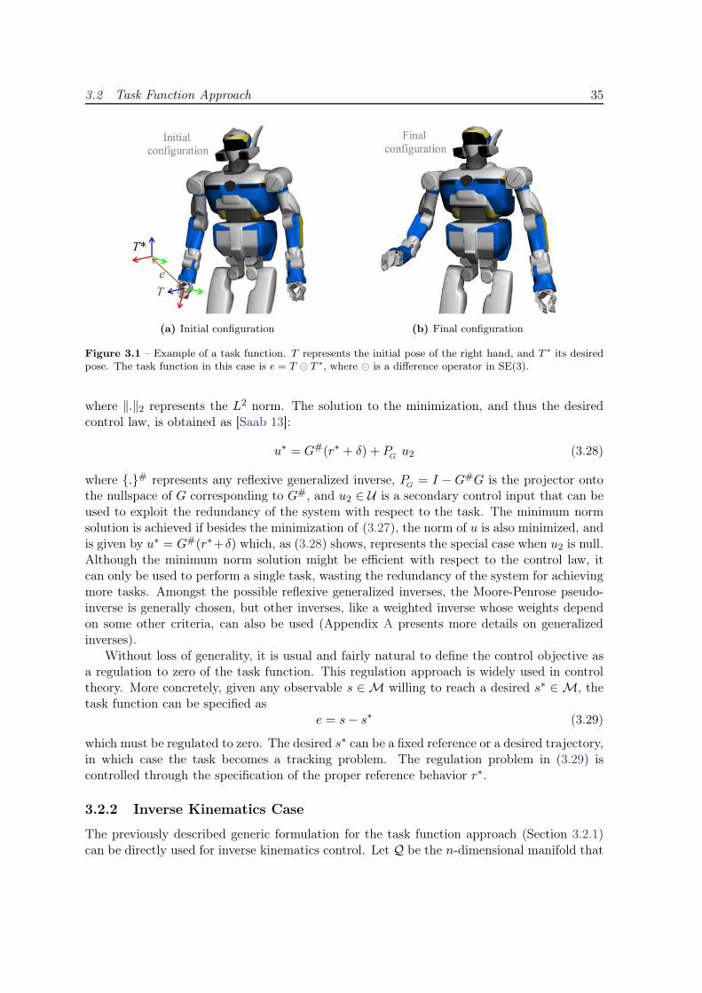
3.2 Task Function Approach 35
(a) Initial configuration (b) Final configuration
Figure 3.1 – Example of a task function. T represents the initial pose of the right hand, and T ∗ its desiredpose. The task function in this case is e = T ⊖ T ∗, where ⊖ is a difference operator in SE(3).
where ‖.‖2 represents the L2 norm. The solution to the minimization, and thus the desiredcontrol law, is obtained as [Saab 13]:
u∗ = G#(r∗ + δ) + PGu2 (3.28)
where {.}# represents any reflexive generalized inverse, PG= I −G#G is the projector onto
the nullspace of G corresponding to G#, and u2 ∈ U is a secondary control input that can beused to exploit the redundancy of the system with respect to the task. The minimum normsolution is achieved if besides the minimization of (3.27), the norm of u is also minimized, andis given by u∗ = G#(r∗+δ) which, as (3.28) shows, represents the special case when u2 is null.Although the minimum norm solution might be efficient with respect to the control law, itcan only be used to perform a single task, wasting the redundancy of the system for achievingmore tasks. Amongst the possible reflexive generalized inverses, the Moore-Penrose pseudo-inverse is generally chosen, but other inverses, like a weighted inverse whose weights dependon some other criteria, can also be used (Appendix A presents more details on generalizedinverses).
Without loss of generality, it is usual and fairly natural to define the control objective asa regulation to zero of the task function. This regulation approach is widely used in controltheory. More concretely, given any observable s ∈ M willing to reach a desired s∗ ∈ M, thetask function can be specified as
e = s− s∗ (3.29)
which must be regulated to zero. The desired s∗ can be a fixed reference or a desired trajectory,in which case the task becomes a tracking problem. The regulation problem in (3.29) iscontrolled through the specification of the proper reference behavior r∗.
3.2.2 Inverse Kinematics Case
The previously described generic formulation for the task function approach (Section 3.2.1)can be directly used for inverse kinematics control. Let Q be the n-dimensional manifold that
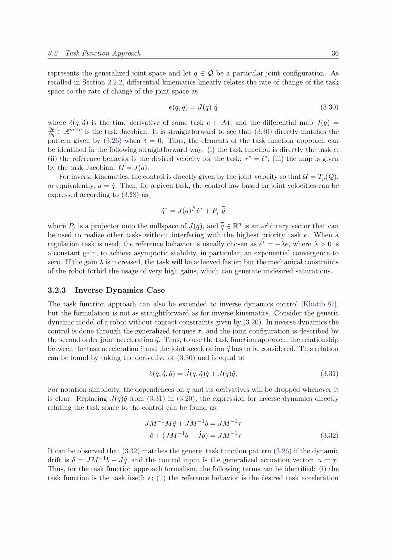
3.2 Task Function Approach 36
represents the generalized joint space and let q ∈ Q be a particular joint configuration. Asrecalled in Section 2.2.2, differential kinematics linearly relates the rate of change of the taskspace to the rate of change of the joint space as
e(q, q) = J(q) q (3.30)
where e(q, q) is the time derivative of some task e ∈ M, and the differential map J(q) =∂e∂q
∈ Rm×n is the task Jacobian. It is straightforward to see that (3.30) directly matches the
pattern given by (3.26) when δ = 0. Thus, the elements of the task function approach canbe identified in the following straightforward way: (i) the task function is directly the task e;(ii) the reference behavior is the desired velocity for the task: r∗ = e∗; (iii) the map is givenby the task Jacobian: G = J(q).
For inverse kinematics, the control is directly given by the joint velocity so that U = Tp(Q),or equivalently, u = q. Then, for a given task, the control law based on joint velocities can beexpressed according to (3.28) as:
q∗ = J(q)#e∗ + PJq
where PJ
is a projector onto the nullspace of J(q), and q ∈ Rn is an arbitrary vector that can
be used to realize other tasks without interfering with the highest priority task e. When aregulation task is used, the reference behavior is usually chosen as e∗ = −λe, where λ > 0 isa constant gain, to achieve asymptotic stability, in particular, an exponential convergence tozero. If the gain λ is increased, the task will be achieved faster; but the mechanical constraintsof the robot forbid the usage of very high gains, which can generate undesired saturations.
3.2.3 Inverse Dynamics Case
The task function approach can also be extended to inverse dynamics control [Khatib 87],but the formulation is not as straightforward as for inverse kinematics. Consider the genericdynamic model of a robot without contact constraints given by (3.20). In inverse dynamics thecontrol is done through the generalized torques τ , and the joint configuration is described bythe second order joint acceleration q. Thus, to use the task function approach, the relationshipbetween the task acceleration e and the joint acceleration q has to be considered. This relationcan be found by taking the derivative of (3.30) and is equal to
e(q, q, q) = J(q, q)q + J(q)q. (3.31)
For notation simplicity, the dependences on q and its derivatives will be dropped whenever itis clear. Replacing J(q)q from (3.31) in (3.20), the expression for inverse dynamics directlyrelating the task space to the control can be found as:
JM−1Mq + JM−1b = JM−1τ
e+ (JM−1b− J q) = JM−1τ (3.32)
It can be observed that (3.32) matches the generic task function pattern (3.26) if the dynamicdrift is δ = JM−1b − J q, and the control input is the generalized actuation vector: u = τ .Thus, for the task function approach formalism, the following terms can be identified: (i) thetask function is the task itself: e; (ii) the reference behavior is the desired task acceleration
3.3 Inverse Dynamics Control 37
r∗ = e∗; (iii) the map is G = JM−1, which is a function of the kinematic differential map(the Jacobian).
The inverse dynamics control is then reduced to finding the desired torque control inputτ∗ that will generate the reference behavior e∗ using any necessary joint accelerations q. Thus,for inverse dynamics, the control law in (3.28) becomes
τ∗ = (JM−1)#(e∗ + JM−1b− J q) + PJM−1
τ
where PJM−1
is a projector onto the nullspace of JM−1 and τ is an arbitrary vector that canbe used to control more tasks with lower priority. The model (3.20) can also be extended tothe case of dynamics with rigid contact constraints and the application of the task-functionapproach leads to similar results [Saab 13].
3.3 Inverse Dynamics Control
The control of reactive humanoid robots in the real world has to deal with constraints imposedby the robot mechanical properties and by the environment. Traditional control based oninverse kinematics only considers kinematical constraints but it does not take into accountany of the other constraints; therefore it is not sufficient and inverse dynamics has to beconsidered. Inverse dynamics control is able to consider the full dynamics of the robot aswell as the environmental constraints and at the same time it can generate different types ofmotion3.
3.3.1 Inverse Dynamics Problem
The inverse dynamics problem consists in finding a control law that will lead to the fulfill-ment of a desired task satisfying the inverse dynamics model of the robot and some addi-tional constraints to ensure the feasibility of the motion. Given a certain task represented byh(q, q, q) = e∗ − e(q, q, q), the inverse dynamics problem can be written in generic form as
minν
‖h(q, q, q)‖2Ns.t. Aν + β = 0
Dν + γ ≥ 0
(3.33)
where ν is the control variable, A, β are matrices defining suitable equality constraints typi-cally given by the dynamic model (3.23) and the kinematic non-holonomic contact constraints(3.3), and D, γ are matrices defining suitable inequality constraints that might represent, forinstance, the unidirectionality of the contact forces (3.4) or (3.8). The minimization is doneusing an N -norm, which can be chosen to control the efforts over the joints [Peters 08]. Ininverse dynamics, the control variable ν must contain the generalized torques τ , but since mo-tion is specified by terms depending on joints acceleration, q can also be included, althoughboth terms are naturally coupled. When the unidirectionality of the forces is considered, fc
3The control framework in this section first appeared in: L. Saab, O. Ramos, N. Mansard, P. Souères, J-Y. Fourquet: Generic Dynamic Motion Generation with Multiple Unilateral Constraints, IEEE InternationalConference on Intelligent Robots and Systems (IROS), San Francisco, CA, USA, September 2011 [Saab 11].
3.3 Inverse Dynamics Control 38
can be included in the control variable ν, but also friction models can be used. Thus, thisgeneric problem for a single task e∗ can be written as
minq,τ,fc
‖e∗ − e(q, q, q)‖2N
s.t. M(q)q + b(q, q) + Jc(q)T fc = ST τ
Jcq + Jcq = 0
f⊥c ≥ 0
(3.34)
There exist two main approaches to solve this problem. The first one aims at determiningan analytical solution through successive projections onto the constraints nullspaces to achievedynamic feasibility. The other one consists in finding the solution treating the problem as apurely optimization problem which allows for the consideration of more generic constraints.
Solutions based on nullspace projections One way to solve the inverse dynamics prob-lem in (3.34) is to consider the constraints analytically and to use the so called projectedinverse-dynamics to eliminate the contact forces. These approaches only consider the equalityconstraints, and inequality constraints cannot be arbitrarily handled. The usage of operationalspace controllers for whole-body control was proposed in [Sentis 05] where the solution is ob-tained using the so-called dynamically consistent Jacobian, which is a particular norm N forthe analytical solution of (3.34). For multiple tasks, this approach uses a prioritization schemebased on projections onto the nullspace of higher priority tasks and constraints. Another ap-proach is based on the orthogonal projections for inverse dynamics introduced in [Aghili 05]and was proposed for legged robots with switching contact constraints in [Mistry 10]. It findsan analytical solution for the torques projecting the robot dynamics onto a reduced dimen-sional space independent of contact forces using the aforementioned orthogonal decompositionand only kinematic projections. Moreover, both approaches have been shown to be equivalentwith respect of different minimization costs [Righetti 11b].
The limitations of these methods are the lack of possibility to include inequality constraintssuch as joint limits, friction cones, amongst others. This leads to obtaining unbounded contactforces which in reality can produce balance problems for a robot, or unfeasible contacts. Also,tasks expressed as inequalities cannot be formulated.
Solutions based on optimization The other approach to solve the inverse dynamicsproblem is to use optimization techniques to find the solution to (3.34). A typical methodis through the usage of Quadratic Programs (QP). The advantage over solutions based onnullspace projections is the ability to handle inequalities such as friction cones, force unidi-rectionality, joint limits or other constraints/tasks. There exist two main approaches in thiscategory when there are more than two tasks to be satisfied at the same time: weightingbased schemes and prioritized schemes.
Weighting-based schemes combine the tasks by assigning a weight αi to each of them. Fornt tasks, the minimization objective of (3.34) becomes
∑nt
i=0 αi‖e∗i − ei‖2. An approach thatis oriented towards robust balance and uses this scheme was proposed in [Collette 08]. Forwhole-body control, the QP formulation based on weighted sums subject to constraints wasproposed in [Bouyarmane 11] and [Salini 11]. The problem with this formulation is the effortneeded to properly tune the weights, and when tasks or constraints conflict with each other,

3.3 Inverse Dynamics Control 39
there can be problems in the solutions: none task is fully satisfied but a compromise amongstthem is obtained.
To solve this problem, prioritized schemes treat the problem as a hierarchy which is anordered list of tasks where lower priority tasks should not interfere with higher priority ones.In these cases, the inverse dynamics problem is recursively solved starting with the highestpriority task and setting the solution of this as a constraint for the next levels. The approach in[deLasa 10] uses a nested sequence of objectives re-parameterized at each level of the hierarchy.An application on a real humanoid robot was implemented in [Herzog 13] using slacks in theQP to account for priority feasibility and reducing the computational cost by decomposingthe equations of motion in the actuated and underactuated parts. Based on this reduction,a framework for this usage in an optimal control scheme outer loop was recently proposed in[Kuindersma 14]. An analytical sparse solution that converts the problem into two smallerindependent unconstrained problems reducing the computational time has been proposed in[DelPrete 14a]. The approach used in this thesis is based on prioritization and for this sake,a cascade of QPs, referred to as hierarchical quadratic program, is used at each level of thehierarchy to handle inequalities at any priority level, which cannot be obtained with otherapproaches.
3.3.2 Hierarchical Quadratic Program (HQP)
The Hierarchical Quadratic Program solver [Escande 14] is an extension of the traditionalQuadratic Program (QP) approach that consists in using a cascade of QPs so that equalities orinequalities, representing constraints, can be handled at any level of the cascade. The cascadeenforces a hierarchy since the constraints corresponding to the first QPs in the cascade willhave a higher priority than the constraints in the next QPs. A constraint with higher priorityis interpreted as a constraint that is satisfied as closely as possible without considering anyother existing (lower-priority) constraints.
Consider a generic prioritized linear system containing N linear equalities or inequalitiesof the following form
di ≤ Aix ≤ di (3.35)
where x is the optimization variable, Ai is a coefficients matrix, di is the lower bound, di isthe upper bound, and i = 1, · · · , N represents the priority in the hierarchy (the lower thevalue of i, the higher the priority). Equalities are a special case of (3.35) when di = di, andsingle-sided inequalities are special cases when di = −∞ (leading to Aix ≤ di) or bi = +∞(leading to Aix ≥ di). An HQP works in the following way. The QP for the first prioritycomponent (i = 1) is written as the optimization problem
minw1,x
‖w1‖22s.t. d1 ≤ A1x+ w1 ≤ d1
where w1 is a slack variable that allows the system to have some freedom in the resolutionin case the exact constraint is not satisfied. The solution to the first priority QP is noted asw∗1, which indirectly represents the best fulfillment of the first constraint. Due to the nature
of the optimization, no other solution lower than w∗1 can be found. However, if the system
is redundant, there is a set of x that achieves the same optimal solution, and it is used to
3.3 Inverse Dynamics Control 40
allow for the resolution of the other lower priority constraints. The second constraint definesa second QP as the problem
minw2,x
‖w2‖22s.t. d2 ≤ A2x+ w2 ≤ d2
d1 ≤ A1x+ w∗1 ≤ d1
where w2 is a slack variable. However, in this case, the minimization is only effectuated forthe second constraint using w2; the variable w∗
1 corresponding to the first constraint is fixedand is the optimized value computed in the previous step. This ensures that the solutionfor the second constraint will not modify the optimal value computed for the first constraint,ensuring a hierarchy. Generalizing the same idea, the QP corresponding to the k-th level ofthe hierarchy can be written as
minwk,x
‖wk‖22s.t. dk ≤ Akx+ wk ≤ dk
d+k−1 ≤ A+k−1x+ w+∗
k−1 ≤ d+k−1
where d+k−1, d+k−1, A
+k−1, and w+∗
k−1 are augmented matrices given by
d+k−1 =
dk−1...d1
d+k−1 =
dk−1...d1
A+k−1 =
Ak−1...A1
w+∗k−1 =
w∗k−1...w∗1
which represent the higher priority constraints, and optimal slack variables (solved in theprevious steps), ranging from i = 1 to i = k − 1.
The previous generic scheme shows that the solution to a system with equalities andinequalities is found using an HQP in such a way that the fact that level k − 1 has higherpriority over level k implies that level k should be fulfilled as close as possible but withoutinterfering with the other higher priority levels: k−1, k−2, · · · , 2, 1. To make the computationfaster, the HQP is solved with a dedicated solver in two steps. First, a classical primal activeset algorithm finds the active inequality constraints and turns them into equalities since thesolution does not change after this reduction. Then, a hierarchized complete orthogonaldecomposition is applied to the set of equalities [Escande 14].
For a system with N linear equalities or inequalities, the HQP hierarchy is usually repre-sented using a lexicographic order as:
(i) ≺ (ii) ≺ (iii) ≺ · · · ≺ (N − 1) ≺ (N) (3.36)
where (i) has the highest priority, and (N) has the lowest priority.
3.3.3 Inverse Dynamics Stack of Tasks (SoT)
For a humanoid robot, different types of motion can be generated using the task functionapproach and satisfying some additional constraints. These constraints arise from the contin-uous contact of the robot with the environment and the fact that balance should be kept at

3.3 Inverse Dynamics Control 41
all instants of time. A robot that achieves a desired task but falls down is useless; thus, thedynamics of the robot must play a highly important role when generating feasible motion.
As stated in Section 3.2, a task can be expressed without loss of generality as the regulationtask (3.29): e = s(q) − s∗. As stated in Section 3.2.3, the dynamic model of the robot usesjoint accelerations, and thus, to use the task function approach, a relation at the accelerationlevel is needed for the control. For a generic task i, the second order differential relationbetween the task space and the joint space is given in a similar way to (3.31) by:
ei = Ji(q, q)q + Ji(q)q (3.37)
where Ji(q) = ∂ei∂q
is the Jacobian of the ith task. Motion for the robot is generated usingseveral instances of (3.37), each specifying an objective, with different priorities dependingon the importance of the task. In fact, the several tasks make the system act like a Stack ofTasks (SoT), and therefore the name. Moreover, tasks can be added or removed at will at anyinstant of time. To enforce feasibility of the motion, the constraints regarding the dynamicmodel (3.23) and the contacts, which using the rigid point contact model are given by (3.3)and (3.4), have to be also considered.
Considering the tasks and the dynamic feasibility constraints, the operational-space inverse-dynamics (OSID) problem can be reduced to finding the optimization vector, sometimes calledthe dynamic variable, as
ν = (q, τ, fc)
which needs to be consistent with the dynamic equations and should minimize the distanceto the task reference. The approach computes at the same time the joint accelerations q,the control torques τ , and the contact forces fc that the robot should apply to the ground.The explicit computation of these variables in the optimization solver has the advantage thatforces are obtained in a straightforward way and no consistency verification or projection isnecessary to guarantee their feasibility. Another advantage is that explicit constraints on eachof the variables can be formulated, as “tasks”, and either a torque-controlled or a position-controlled robot can be used (by integrating q twice). With the lexicographic order introducedin Section 3.3.2, and considering nt tasks of the form (3.37), the dynamic SoT based on theHQP4 is given by
(3.23) ≺ (3.3) ≺ (3.4) ≺ (3.37)-1 ≺ · · · ≺ (3.37)-nt.
where (3.37)-i represents the i-th task of the form (3.37), which is fully specified by thereference behavior e∗i and the Jacobian Ji. To ensure system balance it is generally better toadd sufficient tasks to fill up the SoT, in which case there is no more redundancy to minimizethe torques. But if the SoT is not full, a last task related to ‘joints friction’ or posture (alsoreferred to as damping task) is generally added to complete it [Khatib 04c]. Fig. 3.2 representsgraphically the inverse dynamics Stack of Tasks.
In cases where all the contact points are on a same horizontal plane, the inequality con-dition (3.4), due to its non-negativeness, implies the existence of the ZMP inside the supportpolygon ensuring the dynamic balance of the robot [Saab 13]. Thus, the inverse dynamics con-trol ensures motion generation with dynamic feasibility and respecting the ZMP constraint.
4The approach appears in: L. Saab, O. Ramos, F. Keith, N. Mansard, P. Souères, J-Y. Fourquet, DynamicWhole-Body Motion Generation under Rigid Contacts and other Unilateral Constraints, IEEE Transactionson Robotics (T-RO), Vol.29 N.2, pag. 346 - 362, April 2013 [Saab 13].

3.3 Inverse Dynamics Control 42
Figure 3.2 – Scheme of the Inverse Dynamics Stack of Tasks. The highest priority is at the bottom of thestack. The dynamic consistency and the contact constraints are always satisfied. It should be noted thatcontacts can be pushed or removed from the stack at will. The hierarchy exists at the level of the tasks, whichcan be added or removed as needed. The outputs of the stack are the joint torques, accelerations and thecontact forces, which constitute the optimization variables.
The model used assumes that large friction coefficients are present and, thus, only normalforces are considered instead of more general friction cones. The generalization to frictioncones is straightforward and (3.8) would have to be added to the solver. However, a goodtypical cone approximation uses 12 generators which introduce 12 new variables per contactpoint. This increases the complexity of the HQP solver and thus this approach is not currentlyused due to its computational cost.
3.3.4 Decoupling Motion and Actuation
The variables (q, τ , f) can be decoupled to achieve a faster computation. In fact, the spacegiven by (q, f, τ) in the previous HQP can be divided in three subspaces. The first one isthe motion space, where joint accelerations (q) can be freely chosen, and the correspondingforces (f) and torques (τ) are accordingly set. The second is the actuation space, where theacceleration is fixed and only forces can be freely chosen forasmuch as forces and torques arerelated. The third space is useless since motion variables can be theoretically chosen, butresulting forces are impractical. To explicitly distinguish the actuation space from the motionspace, two decoupled spaces can be introduced. To this end, an automatic formulation hasbeen proposed in [Mansard 12]. This formulation states that instead of using the originaloptimization variables, the bases of the two decoupled spaces can be used and the dynamicmodel as well as the tasks can be reformulated in terms of these decoupled variables. Thisallows a faster computation of the SoT since the decoupled spaces are of lower dimension thanthe original coupled variables.
3.3 Inverse Dynamics Control 43
Decoupled Dynamics
The description presented in this section is a summary of [Mansard 12], which aims at de-coupling the dynamics contained in the dynamic model given by (3.23) as well as the contactconstraints. Using the Cholesky decomposition, the inverse of the inertia matrix M can beexpressed as M−1 = BBT , and thus M = B−TB−1, with B an invertible triangular matrix.Multiplying the dynamic model (3.23) by BT the following expression is obtained
BTST τ = B−1q +BT b+GT fc (3.38)
where G is defined as G = JcB. The result of multiplying (3.38) by G on the left, using (3.3)to guarantee no kinematic motion at the rigid contact point, is
GBTST τ = GBT b+GGT fc − Jcq
where the fact that GB−1q = JcBB−1q = −Jcq, so that xc = 0, has been used. Solving this
expression for BTST τ , it gives:
BTST τ = BT b+GT fc −G#Jcq + V u
where V is a basis of the kernel of G, so that V V T = I − G#G, and u is a vector in thiskernel representing the motion of the system, as (3.42) shows. The term δc = −G# + Jcqcan be associated to the contact drift, and thus, a more compact expression describing theconstrained dynamics can be written as:
BTST τ = BT b+GT fc + δc + V u. (3.39)
An actuation free relation can be obtained if the torque τ is eliminated in (3.39). Tothis end, the matrix S is defined as S = [I 0] in such a way that it cancels out ST , thatis SST = 0, and thus it also eliminates the effect of the torque. Multiplying both terms of(3.39) by SB−T , a torque-free relation between the contact forces fc and the motion term uis obtained:
SB−TV u+ SJTc fc = −Sb− SB−T δc. (3.40)
This expression is composed of both (3.23) and (3.3) but explicitly using the motion (u)and contact force (fc) variables. The other complementarity contact condition related to theunidirectionality of the forces can be directly included in the decoupled model as (3.4) shows,since the contact force is a variable in the model.
Reduction of the Force
It is possible to reduce the force variable as [Mansard 12] proposes. In this case, the contactforce fc can be solved for the system (3.40) giving
fc = −(SJTc )#S(b+B−T δc +B−TV u) +Kψ
where K is a basis of the kernel of SJTc such that KKT = I − (SJTc )#(SJTc ), and ψ is a
vector in this kernel. Since B is triangular, the reduction can further be written as
fc = −(SGT )#S(BT b+ δc + V u) +Kψ. (3.41)
This reduction contains at the same time the inverse dynamics and the kinematic contact con-straint and gives a compact expression that at the same time contains the motion constraintsand the force constraints.
3.3 Inverse Dynamics Control 44
Tasks Representation
A generic task can be typically represented as (3.37), which relates the task acceleration tothe generalized joint space acceleration. The equivalence between (3.38) and (3.39) allows toeliminate the torque component and the contact force component and leads to the relationbetween the acceleration q and u as:
q = Bδc +BV u (3.42)
Therefore, the reduced variable u can be directly associated with the motion q and is usuallyreferred to as the motion variable in the reduced dynamics formulation. Using (3.42), thegeneric task representation (3.37) can be equivalently expressed in terms of the decoupledvariable u as
e∗i = Jiq + JiBδc + JiBV u (3.43)
which is the task formulation in the reduced dynamics framework.
Decoupled Stack of Tasks
The fully decoupled dynamics can be formulated as the following minimization problem.Considering a task i, and using (3.43) and (3.41), the optimization problem is:
minu,ψ
‖ JiBV u+ Jiq + JiBδc − e∗i ‖
s.t. − (SGT )#SV u+Kψ ≥ f0 (3.44)
where the constraint is directly obtained from (3.41), and thus, f0 is typically computed asf0 = −(SGT )#(BT b+ δc). This is the most general decoupled equation and its simplicity canbe observed from the fact that only a single constraint is needed, which already comprisesthe inverse dynamics model as well as the rigid contact conditions. For this system, andconsidering nt tasks, the inverse dynamics SoT can be formulated as
(3.44) ≺ (3.43)-1 ≺ · · · ≺ (3.43)-nt.
An alternative way to solve the system, making explicit the computation of the contactforces is
minu,fc
‖ JiBV u+ Jiq + JiBδc − e∗i ‖
s.t. (SB−TV )u+ (SJTc )fc = −S(b+B−T δc)
f⊥c ≤ 0.
using the lexicographic notation, this system can be written as a hierarchy of nt tasks as
(3.40) ≺ (3.4) ≺ (3.43)-1 ≺ · · · ≺ (3.43)-nt.
The torques can be recovered from (3.39). To this end, the fact that SST = I can beprofitted. Then, multiplying (3.39) by SB−T on the left, the torques are given by
τ = Sb+ SJTc fc + SB−T (δc + V u) (3.45)
and thus, the decoupled dynamics can be used in the computation and the necessary torquescan be then easily computed.
3.4 Tasks for Motion Generation 45
Spatial-force Reduction
Consider a single rigid body i in contact with the environment. The twist associated with acertain reference frame located on the body (for instance, its center of mass) will be denotedby ξ = (v, ω) ∈ se(3), where v represents the linear velocity, and ω the angular velocity. Therelation between this twist and the twist (vk, ωk) ∈ se(3) of a generic point pk on the body(which can be a contact point) is given by:
[
vkωk
]
=
[
I −pk0 I
] [
vω
]
(3.46)
where {.} represents the skew-symmetric matrix of pre-cross product. Let the set of nc contactpoints, where the forces are directly applied, be denoted by xc = (p1, p2, · · · , pnc) ∈ R
3nc , theirvelocity by xc, and their acceleration by xc. Since these points are attached to the rigid body,they do not present angular velocity with respect to it, and further analysis will only considerlinear velocity. Using a direct extension of (3.46), the linear velocity relation is:
xc = X ξ (3.47)
where
xc =
v1v2...vnc
and X =
I3 −p1I3 −p2...I3 −pnc
. (3.48)
Let the geometric Jacobian of the generic frame attached to the body be denoted by Joso that ξ = Jo q. Using this Jacobian, the contact Jacobian (xc = Jcq), and (3.47), it canbe easily verified that the link between the contact Jacobian and the geometric Jacobian isgiven by X, so that
Jc = XJo. (3.49)
When there are 3 or more contact points on the same body, X is full-column rank and thenull spaces of Jc and Jo are equal. In this case, Jo can be used to compute the V basisas V = ker(JoB) instead of V = ker(JcB), and the contact drift as δc = −(JoB)#Joq.However, when there are only 1 or 2 contact points the null spaces are no longer equal. Inthis situation, X in (3.48) is not full-column rank, and the previous reductions where Jo couldbe used instead of Jc do not necessarily hold since both matrices do not have the same nullspace. In this case, the equivalence Jc = XJo is used and the computation of V is explicitlyker(XJoB). The relation between the derivative of both Jacobians is Jc = XJo + XJo, butthe second term is null (X is null provided that the contact points do not move) leading toJc = XJo. Then, for the contact drift in the generic case, δc = −(XJoB)#XJoq.
3.4 Tasks for Motion Generation
Motion generation within the dynamic SoT is based upon the definition and usage of differenttasks at the acceleration level. These tasks5 are completely specified through the task reference
5Some of these tasks appear in: L. Saab, O. Ramos, F. Keith, N. Mansard, P. Souères, J-Y. Fourquet,Dynamic Whole-Body Motion Generation under Rigid Contacts and other Unilateral Constraints, IEEE Trans-actions on Robotics (T-RO), Vol.29 N.2, pag. 346 - 362, April 2013 [Saab 13].
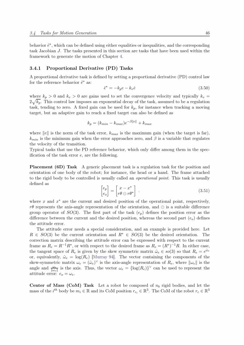
3.4 Tasks for Motion Generation 46
behavior e∗, which can be defined using either equalities or inequalities, and the correspondingtask Jacobian J . The tasks presented in this section are tasks that have been used within theframework to generate the motion of Chapter 4.
3.4.1 Proportional Derivative (PD) Tasks
A proportional derivative task is defined by setting a proportional derivative (PD) control lawfor the reference behavior e∗ as:
e∗ = −kpe− kv e (3.50)
where kp > 0 and kv > 0 are gains used to set the convergence velocity and typically kv =2√
kp. This control law imposes an exponential decay of the task, assumed to be a regulationtask, tending to zero. A fixed gain can be used for kp, for instance when tracking a movingtarget, but an adaptive gain to reach a fixed target can also be defined as
kp = (kmin − kmax)e−β‖e‖ + kmax
where ‖e‖ is the norm of the task error, kmax is the maximum gain (when the target is far),kmin is the minimum gain when the error approaches zero, and β is a variable that regulatesthe velocity of the transition.Typical tasks that use the PD reference behavior, which only differ among them in the spec-ification of the task error e, are the following.
Placement (6D) Task A generic placement task is a regulation task for the position andorientation of one body of the robot; for instance, the head or a hand. The frame attachedto the rigid body to be controlled is usually called an operational point. This task is usuallydefined as
[
epeo
]
=
[
x− x∗
rθ ⊖ rθ∗
]
. (3.51)
where x and x∗ are the current and desired position of the operational point, respectively,rθ represents the axis-angle representation of the orientation, and ⊖ is a suitable differencegroup operator of SO(3). The first part of the task (ep) defines the position error as thedifference between the current and the desired position, whereas the second part (eo) definesthe attitude error.
The attitude error needs a special consideration, and an example is provided here. LetR ∈ SO(3) be the current orientation and R∗ ∈ SO(3) be the desired orientation. Thecorrection matrix describing the attitude error can be expressed with respect to the currentframe as Re = R−1R∗, or with respect to the desired frame as Re = (R∗)−1R. In either case,the tangent space of Re is given by the skew symmetric matrix ωe ∈ so(3) so that Re = eωe
or, equivalently, ωe = log(Re) [Murray 94]. The vector containing the components of theskew-symmetric matrix ωe = (ωe)
∨ is the axis-angle representation of Re, where ‖ωe‖ is theangle and ωe
‖ωe‖is the axis. Thus, the vector ωe = {log(Re)}∨ can be used to represent the
attitude error: eo = ωe.
Center of Mass (CoM) Task Let a robot be composed of nb rigid bodies, and let themass of the ith body be mi ∈ R and its CoM position rci ∈ R
3. The CoM of the robot rc ∈ R3
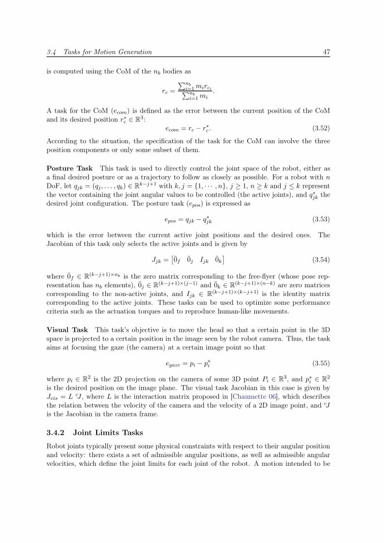
3.4 Tasks for Motion Generation 47
is computed using the CoM of the nb bodies as
rc =
∑nb
i=1mirci∑nb
i=1mi.
A task for the CoM (ecom) is defined as the error between the current position of the CoMand its desired position r∗c ∈ R
3:ecom = rc − r∗c . (3.52)
According to the situation, the specification of the task for the CoM can involve the threeposition components or only some subset of them.
Posture Task This task is used to directly control the joint space of the robot, either asa final desired posture or as a trajectory to follow as closely as possible. For a robot with nDoF, let qjk = (qj, . . . , qk) ∈ R
k−j+1 with k, j = {1, · · · , n}, j ≥ 1, n ≥ k and j ≤ k representthe vector containing the joint angular values to be controlled (the active joints), and q∗jk thedesired joint configuration. The posture task (epos) is expressed as
epos = qjk − q∗jk (3.53)
which is the error between the current active joint positions and the desired ones. TheJacobian of this task only selects the active joints and is given by
Jjk =[
0f 0j Ijk 0k]
(3.54)
where 0f ∈ R(k−j+1)×nb is the zero matrix corresponding to the free-flyer (whose pose rep-
resentation has nb elements), 0j ∈ R(k−j+1)×(j−1) and 0k ∈ R
(k−j+1)×(n−k) are zero matricescorresponding to the non-active joints, and Ijk ∈ R
(k−j+1)×(k−j+1) is the identity matrixcorresponding to the active joints. These tasks can be used to optimize some performancecriteria such as the actuation torques and to reproduce human-like movements.
Visual Task This task’s objective is to move the head so that a certain point in the 3Dspace is projected to a certain position in the image seen by the robot camera. Thus, the taskaims at focusing the gaze (the camera) at a certain image point so that
egaze = pi − p∗i (3.55)
where pi ∈ R2 is the 2D projection on the camera of some 3D point Pi ∈ R
3, and p∗i ∈ R2
is the desired position on the image plane. The visual task Jacobian in this case is given byJvis = L cJ , where L is the interaction matrix proposed in [Chaumette 06], which describesthe relation between the velocity of the camera and the velocity of a 2D image point, and cJis the Jacobian in the camera frame.
3.4.2 Joint Limits Tasks
Robot joints typically present some physical constraints with respect to their angular positionand velocity: there exists a set of admissible angular positions, as well as admissible angularvelocities, which define the joint limits for each joint of the robot. A motion intended to be
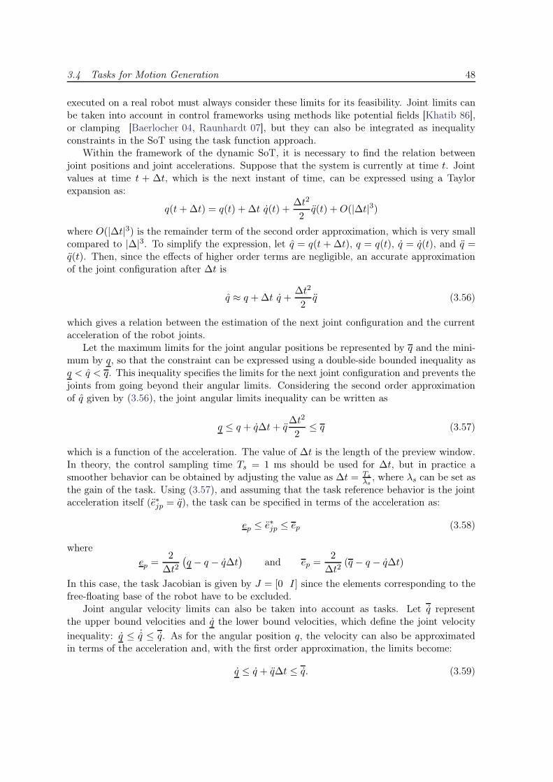
3.4 Tasks for Motion Generation 48
executed on a real robot must always consider these limits for its feasibility. Joint limits canbe taken into account in control frameworks using methods like potential fields [Khatib 86],or clamping [Baerlocher 04, Raunhardt 07], but they can also be integrated as inequalityconstraints in the SoT using the task function approach.
Within the framework of the dynamic SoT, it is necessary to find the relation betweenjoint positions and joint accelerations. Suppose that the system is currently at time t. Jointvalues at time t + ∆t, which is the next instant of time, can be expressed using a Taylorexpansion as:
q(t+∆t) = q(t) + ∆t q(t) +∆t2
2q(t) +O(|∆t|3)
where O(|∆t|3) is the remainder term of the second order approximation, which is very smallcompared to |∆|3. To simplify the expression, let q = q(t +∆t), q = q(t), q = q(t), and q =q(t). Then, since the effects of higher order terms are negligible, an accurate approximationof the joint configuration after ∆t is
q ≈ q +∆t q +∆t2
2q (3.56)
which gives a relation between the estimation of the next joint configuration and the currentacceleration of the robot joints.
Let the maximum limits for the joint angular positions be represented by q and the mini-mum by q, so that the constraint can be expressed using a double-side bounded inequality asq < q < q. This inequality specifies the limits for the next joint configuration and prevents thejoints from going beyond their angular limits. Considering the second order approximationof q given by (3.56), the joint angular limits inequality can be written as
q ≤ q + q∆t+ q∆t2
2≤ q (3.57)
which is a function of the acceleration. The value of ∆t is the length of the preview window.In theory, the control sampling time Ts = 1 ms should be used for ∆t, but in practice asmoother behavior can be obtained by adjusting the value as ∆t = Ts
λs, where λs can be set as
the gain of the task. Using (3.57), and assuming that the task reference behavior is the jointacceleration itself (e∗jp = q), the task can be specified in terms of the acceleration as:
ep ≤ e∗jp ≤ ep (3.58)
where
ep =2
∆t2(
q − q − q∆t)
and ep =2
∆t2(q − q − q∆t)
In this case, the task Jacobian is given by J = [0 I] since the elements corresponding to thefree-floating base of the robot have to be excluded.
Joint angular velocity limits can also be taken into account as tasks. Let q representthe upper bound velocities and q the lower bound velocities, which define the joint velocity
inequality: q ≤ ˙q ≤ q. As for the angular position q, the velocity can also be approximatedin terms of the acceleration and, with the first order approximation, the limits become:
q ≤ q + q∆t ≤ q. (3.59)
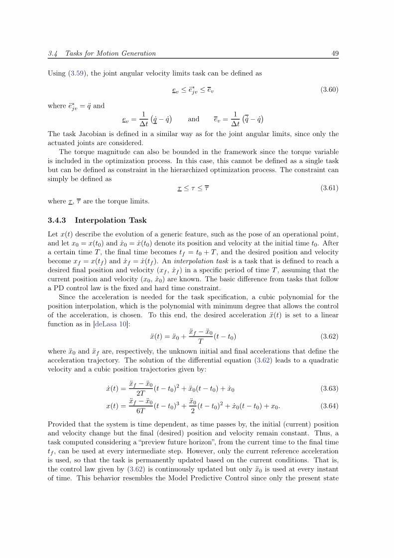
3.4 Tasks for Motion Generation 49
Using (3.59), the joint angular velocity limits task can be defined as
ev ≤ e∗jv ≤ ev (3.60)
where e∗jv = q and
ev =1
∆t
(
q − q)
and ev =1
∆t
(
q − q)
The task Jacobian is defined in a similar way as for the joint angular limits, since only theactuated joints are considered.
The torque magnitude can also be bounded in the framework since the torque variableis included in the optimization process. In this case, this cannot be defined as a single taskbut can be defined as constraint in the hierarchized optimization process. The constraint cansimply be defined as
τ ≤ τ ≤ τ (3.61)
where τ , τ are the torque limits.
3.4.3 Interpolation Task
Let x(t) describe the evolution of a generic feature, such as the pose of an operational point,and let x0 = x(t0) and x0 = x(t0) denote its position and velocity at the initial time t0. Aftera certain time T , the final time becomes tf = t0 + T , and the desired position and velocitybecome xf = x(tf ) and xf = x(tf ). An interpolation task is a task that is defined to reach adesired final position and velocity (xf , xf ) in a specific period of time T , assuming that thecurrent position and velocity (x0, x0) are known. The basic difference from tasks that followa PD control law is the fixed and hard time constraint.
Since the acceleration is needed for the task specification, a cubic polynomial for theposition interpolation, which is the polynomial with minimum degree that allows the controlof the acceleration, is chosen. To this end, the desired acceleration x(t) is set to a linearfunction as in [deLasa 10]:
x(t) = x0 +xf − x0T
(t− t0) (3.62)
where x0 and xf are, respectively, the unknown initial and final accelerations that define theacceleration trajectory. The solution of the differential equation (3.62) leads to a quadraticvelocity and a cubic position trajectories given by:
x(t) =xf − x0
2T(t− t0)
2 + x0(t− t0) + x0 (3.63)
x(t) =xf − x0
6T(t− t0)
3 +x02(t− t0)
2 + x0(t− t0) + x0. (3.64)
Provided that the system is time dependent, as time passes by, the initial (current) positionand velocity change but the final (desired) position and velocity remain constant. Thus, atask computed considering a “preview future horizon”, from the current time to the final timetf , can be used at every intermediate step. However, only the current reference accelerationis used, so that the task is permanently updated based on the current conditions. That is,the control law given by (3.62) is continuously updated but only x0 is used at every instantof time. This behavior resembles the Model Predictive Control since only the present state
3.4 Tasks for Motion Generation 50
is used although the whole time horizon has been computed. The dynamic task can thus besimply defined as e∗ = x0, and can be obtained by solving the system (3.63) and (3.64) attime t = tf leading to the following desired reference behavior:
e∗ =6
T 2(xf − x0)−
2
T(xf + 2x0). (3.65)
It should be noted that T becomes smaller after each iteration and is close to zero when theinitial time reaches the final time. This situation can be handled by keeping the previousvalue of x0 when T < th, where th is a threshold. In practice, keeping the previous value ofthe acceleration gives good results.
3.4.4 Capture Point (CP) Task
The Capture Point (CP), introduced in [Pratt 06b] and also referred to as the ExtrapolatedCenter of Mass [Hof 05], is the point ξ = [ξx ξy 0]T on the ground where the robot shouldstep on to be able to come to a complete rest. It is based on modeling the robot as a linearinverted pendulum (LIP) [Pratt 06a]. Let the position of the robot CoM be represented byrc = (xc, yc, zc), so that the horizontal component of the CoM is rc = n × rc × n, withn = (0, 0, 1), or equivalently, rc = (xc, yc, 0). It can be shown (see Appendix C for moredetails) that the instantaneous Capture Point is given by
ξ = rc +˙rcω
(3.66)
where ω =√
gzc
is the eigenfrequency of the pendulum that models the robot dynamics.
The CP task6 is proposed as an inequality task that aims at keeping the CP inside certainlimits at all times. These limits can be the robot support polygon, in which case the robotmotion can come to a stop without needing a step, or an exterior polygon. In the latter casethe robot needs to perform a step, but the motion can be constrained so that the CP stayswithin some reachable region for the leg. In both cases, the task is bounded by a genericpolygon. Let the limits of the generic polygon be given by rp and rp. The CP must lie withinthe limits of this polygon as:
rp ≤ ξ ≤ rp
rp ≤ rc +˙rcω
≤ rp. (3.67)
From (3.67), it is evident that the CP can be bounded by indirectly controlling the CoMposition and velocity. Then, the task to effectively control the CP can be defined in terms ofthe CoM. Since tasks are integrated in a dynamic control scheme, the CP task needs to beformulated using the acceleration; hence, rc and ˙rc in (3.67) need to be related to the CoMacceleration. As for the case of the joint limits, presented in Section 3.4.2, the position of theCoM can be expressed, using a Taylor series development around point rci , as:
rc = rci +˙rci∆t+
¨rci∆t2
26The CP task was introduced in: O. Ramos, N. Mansard, P. Souères, Whole-body Motion Integrating the
Capture Point in the Operational Space Inverse Dynamics Control, IEEE-RAS International Conference onHumanoid Robots (Humanoids), Madrid, Spain, November 2014 [Ramos 14b].
3.5 Conclusion 51
and the velocity as˙rc = ˙rci +
¨rci∆t.
Replacing the Taylor expansion of the position and the velocity of the CoM in (3.67), andletting the task reference behavior be e∗cp = ¨rci , the Capture Point task respecting the limitswithin the polygon is expressed as a function of the CoM as:
ka ec ≤ e∗cp ≤ ka ec (3.68)
where ka is a constant given by
ka =2ω
∆t(ω∆t+ 2)
and the acceleration limits are
ec = rsp − rci − ˙rci
(
∆t+1
ω
)
ec = rsp − rci − ˙rci
(
∆t+1
ω
)
.
3.5 Conclusion
Based on the task function approach, this chapter has presented the operational-space inverse-dynamics control framework that is used throughout this thesis. A hierarchical QP wasproposed to solve the inverse dynamics problem and give a solution to the tasks generatingwhole-body motion that satisfies the dynamic constraints. Finally, several tasks defined asequalities or inequalities, which can be used at any level of the hierarchy to achieve the desiredeffect, were proposed as the basis for motion generation.
Chapter 4
Case Studies
The whole-body motion generation described in Chapter 3 can be applied to different experi-ments with the robot. This chapter presents different case studies where the motion generationusing the operational-space inverse-dynamics (OSID) stack of tasks (SoT) has been success-fully applied to show and explore some of the possibilities that it can offer. The case studiesshow results obtained both in simulation, using the dynamic model of HRP-2, and in realityusing the robot.
4.1 Motion with Multiple Non-coplanar Contacts
The first case study illustrates the possibility of multiple non-coplanar contacts during acomplex sequence of motions. It consists on two specific motions: the first one presents thereal HRP-2 sitting down in an armchair, and the second one presents the simulated Romeorobot climbing a ladder. The ability to handle multiple non-coplanar contacts is an advantageof the proposed methodology over other existing inverse dynamics approaches and is exploitedin this section.
4.1.1 Sitting in an Armchair
In this sequence of movements, HRP-2 moves its whole-body to sit in an armchair as Fig. 4.1shows1. The robot does not only have both feet in contact with the ground but gradually thecontacts of the hands and the armrests are added and taken into account in the solver. Thehigh-level description of the motion is the following:
• First, the robot looks left and moves its left arm towards the left armrest so that contactsbetween the left gripper and the left chair armrest are found (Fig. 4.1b).
1This experiment appears in: L. Saab, O. Ramos, F. Keith, N. Mansard, P. Souères, J-Y. Fourquet, Dy-namic Whole-Body Motion Generation under Rigid Contacts and other Unilateral Constraints, IEEE Trans-actions on Robotics (T-RO), Vol.29 N.2, pag. 346 - 362, April 2013 [Saab 13].
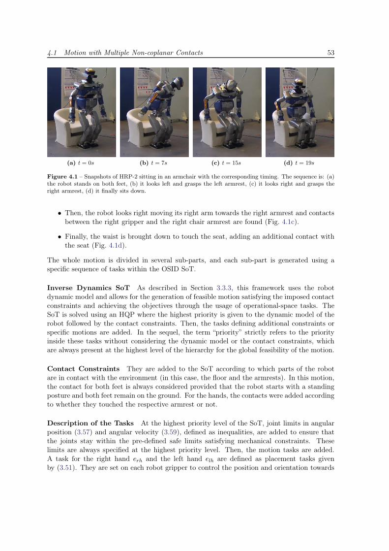
4.1 Motion with Multiple Non-coplanar Contacts 53
(a) t = 0s (b) t = 7s (c) t = 15s (d) t = 19s
Figure 4.1 – Snapshots of HRP-2 sitting in an armchair with the corresponding timing. The sequence is: (a)the robot stands on both feet, (b) it looks left and grasps the left armrest, (c) it looks right and grasps theright armrest, (d) it finally sits down.
• Then, the robot looks right moving its right arm towards the right armrest and contactsbetween the right gripper and the right chair armrest are found (Fig. 4.1c).
• Finally, the waist is brought down to touch the seat, adding an additional contact withthe seat (Fig. 4.1d).
The whole motion is divided in several sub-parts, and each sub-part is generated using aspecific sequence of tasks within the OSID SoT.
Inverse Dynamics SoT As described in Section 3.3.3, this framework uses the robotdynamic model and allows for the generation of feasible motion satisfying the imposed contactconstraints and achieving the objectives through the usage of operational-space tasks. TheSoT is solved using an HQP where the highest priority is given to the dynamic model of therobot followed by the contact constraints. Then, the tasks defining additional constraints orspecific motions are added. In the sequel, the term “priority” strictly refers to the priorityinside these tasks without considering the dynamic model or the contact constraints, whichare always present at the highest level of the hierarchy for the global feasibility of the motion.
Contact Constraints They are added to the SoT according to which parts of the robotare in contact with the environment (in this case, the floor and the armrests). In this motion,the contact for both feet is always considered provided that the robot starts with a standingposture and both feet remain on the ground. For the hands, the contacts were added accordingto whether they touched the respective armrest or not.
Description of the Tasks At the highest priority level of the SoT, joint limits in angularposition (3.57) and angular velocity (3.59), defined as inequalities, are added to ensure thatthe joints stay within the pre-defined safe limits satisfying mechanical constraints. Theselimits are always specified at the highest priority level. Then, the motion tasks are added.A task for the right hand erh and the left hand elh are defined as placement tasks givenby (3.51). They are set on each robot gripper to control the position and orientation towards
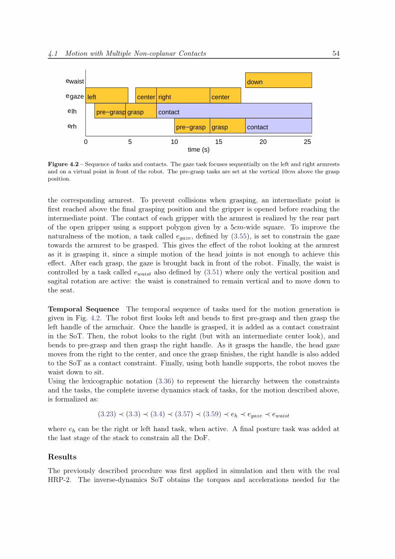
4.1 Motion with Multiple Non-coplanar Contacts 54
0 5 10 15 20 25
rh e
lh e
gazee
waiste
time (s)
pre−grasp grasp contact
pre−grasp grasp contact
left center right center
down
Figure 4.2 – Sequence of tasks and contacts. The gaze task focuses sequentially on the left and right armrestsand on a virtual point in front of the robot. The pre-grasp tasks are set at the vertical 10cm above the graspposition.
the corresponding armrest. To prevent collisions when grasping, an intermediate point isfirst reached above the final grasping position and the gripper is opened before reaching theintermediate point. The contact of each gripper with the armrest is realized by the rear partof the open gripper using a support polygon given by a 5cm-wide square. To improve thenaturalness of the motion, a task called egaze, defined by (3.55), is set to constrain the gazetowards the armrest to be grasped. This gives the effect of the robot looking at the armrestas it is grasping it, since a simple motion of the head joints is not enough to achieve thiseffect. After each grasp, the gaze is brought back in front of the robot. Finally, the waist iscontrolled by a task called ewaist also defined by (3.51) where only the vertical position andsagital rotation are active: the waist is constrained to remain vertical and to move down tothe seat.
Temporal Sequence The temporal sequence of tasks used for the motion generation isgiven in Fig. 4.2. The robot first looks left and bends to first pre-grasp and then grasp theleft handle of the armchair. Once the handle is grasped, it is added as a contact constraintin the SoT. Then, the robot looks to the right (but with an intermediate center look), andbends to pre-grasp and then grasp the right handle. As it grasps the handle, the head gazemoves from the right to the center, and once the grasp finishes, the right handle is also addedto the SoT as a contact constraint. Finally, using both handle supports, the robot moves thewaist down to sit.Using the lexicographic notation (3.36) to represent the hierarchy between the constraintsand the tasks, the complete inverse dynamics stack of tasks, for the motion described above,is formalized as:
(3.23) ≺ (3.3) ≺ (3.4) ≺ (3.57) ≺ (3.59) ≺ eh ≺ egaze ≺ ewaist
where eh can be the right or left hand task, when active. A final posture task was added atthe last stage of the stack to constrain all the DoF.
Results
The previously described procedure was first applied in simulation and then with the realHRP-2. The inverse-dynamics SoT obtains the torques and accelerations needed for the
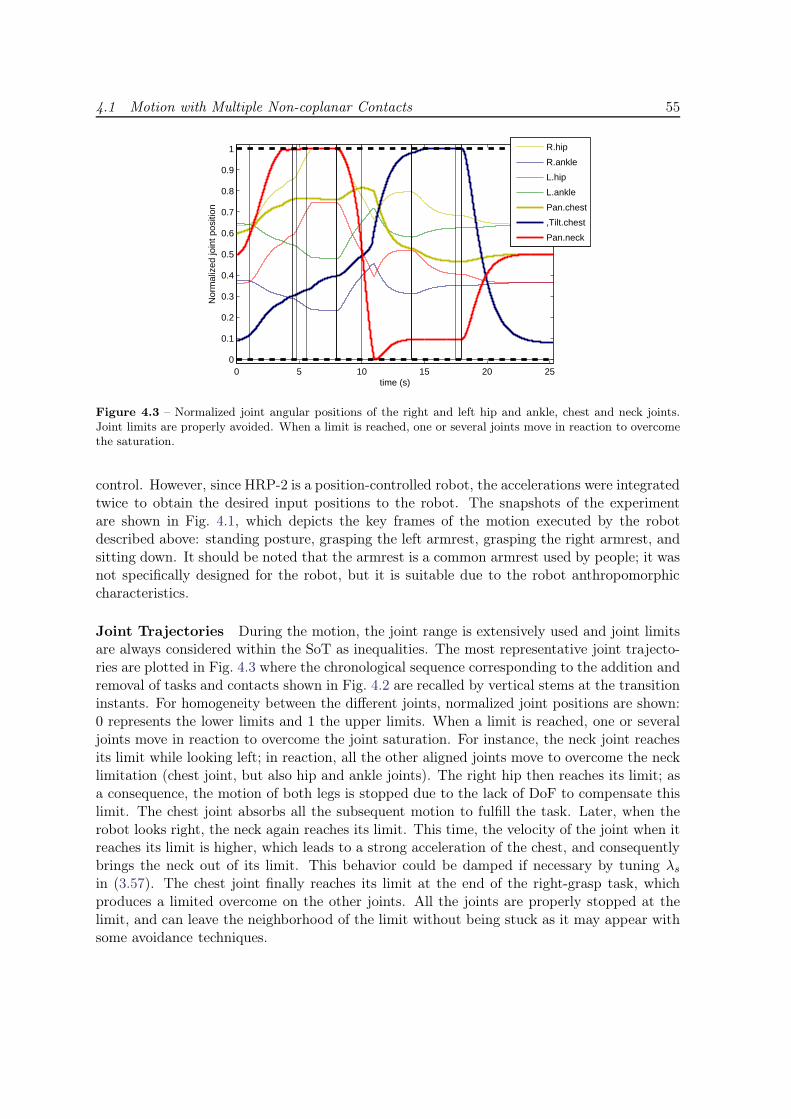
4.1 Motion with Multiple Non-coplanar Contacts 55
0 5 10 15 20 250
0.1
0.2
0.3
0.4
0.5
0.6
0.7
0.8
0.9
1
time (s)
Nor
mal
ized
join
t pos
ition
R.hip
R.ankle
L.hip
L.ankle
Pan.chest
,Tilt.chest
Pan.neck
Figure 4.3 – Normalized joint angular positions of the right and left hip and ankle, chest and neck joints.Joint limits are properly avoided. When a limit is reached, one or several joints move in reaction to overcomethe saturation.
control. However, since HRP-2 is a position-controlled robot, the accelerations were integratedtwice to obtain the desired input positions to the robot. The snapshots of the experimentare shown in Fig. 4.1, which depicts the key frames of the motion executed by the robotdescribed above: standing posture, grasping the left armrest, grasping the right armrest, andsitting down. It should be noted that the armrest is a common armrest used by people; it wasnot specifically designed for the robot, but it is suitable due to the robot anthropomorphiccharacteristics.
Joint Trajectories During the motion, the joint range is extensively used and joint limitsare always considered within the SoT as inequalities. The most representative joint trajecto-ries are plotted in Fig. 4.3 where the chronological sequence corresponding to the addition andremoval of tasks and contacts shown in Fig. 4.2 are recalled by vertical stems at the transitioninstants. For homogeneity between the different joints, normalized joint positions are shown:0 represents the lower limits and 1 the upper limits. When a limit is reached, one or severaljoints move in reaction to overcome the joint saturation. For instance, the neck joint reachesits limit while looking left; in reaction, all the other aligned joints move to overcome the necklimitation (chest joint, but also hip and ankle joints). The right hip then reaches its limit; asa consequence, the motion of both legs is stopped due to the lack of DoF to compensate thislimit. The chest joint absorbs all the subsequent motion to fulfill the task. Later, when therobot looks right, the neck again reaches its limit. This time, the velocity of the joint when itreaches its limit is higher, which leads to a strong acceleration of the chest, and consequentlybrings the neck out of its limit. This behavior could be damped if necessary by tuning λsin (3.57). The chest joint finally reaches its limit at the end of the right-grasp task, whichproduces a limited overcome on the other joints. All the joints are properly stopped at thelimit, and can leave the neighborhood of the limit without being stuck as it may appear withsome avoidance techniques.
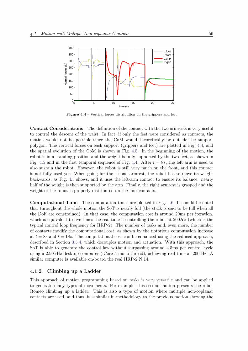
4.1 Motion with Multiple Non-coplanar Contacts 56
0 5 10 15 20 250
50
100
150
200
250
300
350
400
time (s)
Nor
mal
forc
es (
N)
L.footR.footL.gripR.grip
Figure 4.4 – Vertical forces distribution on the grippers and feet
Contact Considerations The definition of the contact with the two armrests is very usefulto control the descent of the waist. In fact, if only the feet were considered as contacts, themotion would not be possible since the CoM would theoretically be outside the supportpolygon. The vertical forces on each support (grippers and feet) are plotted in Fig. 4.4, andthe spatial evolution of the CoM is shown in Fig. 4.5. In the beginning of the motion, therobot is in a standing position and the weight is fully supported by the two feet, as shown inFig. 4.5 and in the first temporal sequence of Fig. 4.4. After t = 8s, the left arm is used toalso sustain the robot. However, the robot is still very much on the front, and this contactis not fully used yet. When going for the second armrest, the robot has to move its weightbackwards, as Fig. 4.5 shows, and it uses the left-arm contact to ensure its balance: nearlyhalf of the weight is then supported by the arm. Finally, the right armrest is grasped and theweight of the robot is properly distributed on the four contacts.
Computational Time The computation times are plotted in Fig. 4.6. It should be notedthat throughout the whole motion the SoT is nearly full (the stack is said to be full when allthe DoF are constrained). In that case, the computation cost is around 20ms per iteration,which is equivalent to five times the real time if controlling the robot at 200Hz (which is thetypical control loop frequency for HRP-2). The number of tasks and, even more, the numberof contacts modify the computational cost, as shown by the notorious computation increaseat t = 8s and t = 18s. The computational cost can be enhanced using the reduced approach,described in Section 3.3.4, which decouples motion and actuation. With this approach, theSoT is able to generate the control law without surpassing around 4.5ms per control cycleusing a 2.9 GHz desktop computer (iCore 5 mono thread), achieving real time at 200 Hz. Asimilar computer is available on-board the real HRP-2 N.14.
4.1.2 Climbing up a Ladder
This approach of motion programming based on tasks is very versatile and can be appliedto generate many types of movements. For example, this second motion presents the robotRomeo climbing up a ladder. This is also a type of motion where multiple non-coplanarcontacts are used, and thus, it is similar in methodology to the previous motion showing the
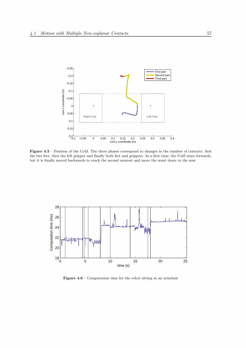
4.1 Motion with Multiple Non-coplanar Contacts 57
−0.25
−0.2
−0.15
−0.1
−0.05
0
0.05
0.1
0.15
0.2−0.1 −0.05 0 0.05 0.1 0.15 0.2 0.25 0.3 0.35 0.4
com
x c
oord
inat
e (m
)
com y coordinate (m)
Left FootRight Foot
First partSecond partThird part
Figure 4.5 – Position of the CoM. The three phases correspond to changes in the number of contacts: firstthe two feet, then the left gripper and finally both feet and grippers. In a first time, the CoM stays forwards,but it is finally moved backwards to reach the second armrest and move the waist down to the seat.
0 5 10 15 20 2518
20
22
24
26
28
time (s)
Com
puta
tion
time
(ms)
Figure 4.6 – Computation time for the robot sitting in an armchair
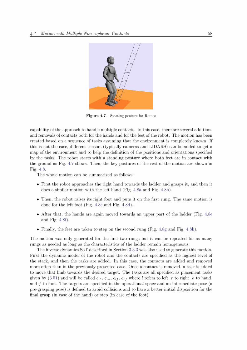
4.1 Motion with Multiple Non-coplanar Contacts 58
Figure 4.7 – Starting posture for Romeo
capability of the approach to handle multiple contacts. In this case, there are several additionsand removals of contacts both for the hands and for the feet of the robot. The motion has beencreated based on a sequence of tasks assuming that the environment is completely known. Ifthis is not the case, different sensors (typically cameras and LIDARS) can be added to get amap of the environment and to help the definition of the positions and orientations specifiedby the tasks. The robot starts with a standing posture where both feet are in contact withthe ground as Fig. 4.7 shows. Then, the key postures of the rest of the motion are shown inFig. 4.8.
The whole motion can be summarized as follows:
• First the robot approaches the right hand towards the ladder and grasps it, and then itdoes a similar motion with the left hand (Fig. 4.8a and Fig. 4.8b).
• Then, the robot raises its right foot and puts it on the first rung. The same motion isdone for the left foot (Fig. 4.8c and Fig. 4.8d).
• After that, the hands are again moved towards an upper part of the ladder (Fig. 4.8eand Fig. 4.8f).
• Finally, the feet are taken to step on the second rung (Fig. 4.8g and Fig. 4.8h).
The motion was only generated for the first two rungs but it can be repeated for as manyrungs as needed as long as the characteristics of the ladder remain homogeneous.
The inverse dynamics SoT described in Section 3.3.3 was also used to generate this motion.First the dynamic model of the robot and the contacts are specified as the highest level ofthe stack, and then the tasks are added. In this case, the contacts are added and removedmore often than in the previously presented case. Once a contact is removed, a task is addedto move that limb towards the desired target. The tasks are all specified as placement tasksgiven by (3.51) and will be called elh, erh, elf , erf where l refers to left, r to right, h to hand,and f to foot. The targets are specified in the operational space and an intermediate pose (apre-grasping pose) is defined to avoid collisions and to have a better initial disposition for thefinal grasp (in case of the hand) or step (in case of the foot).
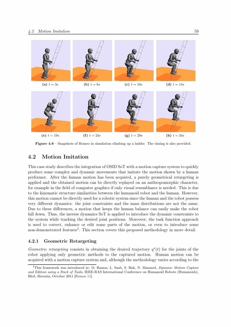
4.2 Motion Imitation 59
(a) t = 3s (b) t = 6s (c) t = 10s (d) t = 14s
(e) t = 19s (f) t = 24s (g) t = 29s (h) t = 34s
Figure 4.8 – Snapshots of Romeo in simulation climbing up a ladder. The timing is also provided.
4.2 Motion Imitation
This case study describes the integration of OSID SoT with a motion capture system to quicklyproduce some complex and dynamic movements that imitate the motion shown by a humanperformer. After the human motion has been acquired, a purely geometrical retargeting isapplied and the obtained motion can be directly replayed on an anthropomorphic character,for example in the field of computer graphics if only visual resemblance is needed. This is dueto the kinematic structure similarities between the humanoid robot and the human. However,this motion cannot be directly used for a robotic system since the human and the robot possessvery different dynamics: the joint constraints and the mass distributions are not the same.Due to these differences, a motion that keeps the human balance can easily make the robotfall down. Thus, the inverse dynamics SoT is applied to introduce the dynamic constraints tothe system while tracking the desired joint positions. Moreover, the task function approachis used to correct, enhance or edit some parts of the motion, or even to introduce somenon-demonstrated features2. This section covers this proposed methodology in more detail.
4.2.1 Geometric Retargeting
Geometric retargeting consists in obtaining the desired trajectory q∗(t) for the joints of therobot applying only geometric methods to the captured motion. Human motion can beacquired with a motion capture system and, although the methodology varies according to the
2This framework was introduced in: O. Ramos, L. Saab, S. Hak, N. Mansard, Dynamic Motion Captureand Edition using a Stack of Tasks, IEEE-RAS International Conference on Humanoid Robots (Humanoids),Bled, Slovenia, October 2011 [Ramos 11].
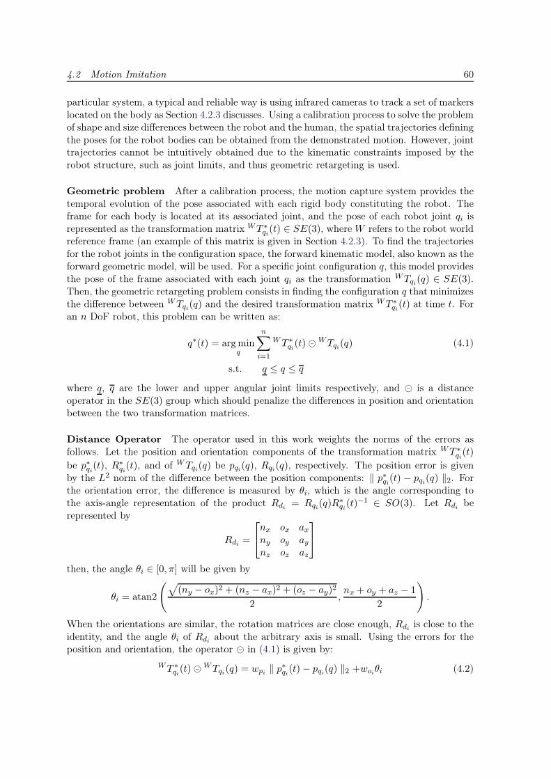
4.2 Motion Imitation 60
particular system, a typical and reliable way is using infrared cameras to track a set of markerslocated on the body as Section 4.2.3 discusses. Using a calibration process to solve the problemof shape and size differences between the robot and the human, the spatial trajectories definingthe poses for the robot bodies can be obtained from the demonstrated motion. However, jointtrajectories cannot be intuitively obtained due to the kinematic constraints imposed by therobot structure, such as joint limits, and thus geometric retargeting is used.
Geometric problem After a calibration process, the motion capture system provides thetemporal evolution of the pose associated with each rigid body constituting the robot. Theframe for each body is located at its associated joint, and the pose of each robot joint qi isrepresented as the transformation matrix WT ∗
qi(t) ∈ SE(3), where W refers to the robot world
reference frame (an example of this matrix is given in Section 4.2.3). To find the trajectoriesfor the robot joints in the configuration space, the forward kinematic model, also known as theforward geometric model, will be used. For a specific joint configuration q, this model providesthe pose of the frame associated with each joint qi as the transformation WTqi(q) ∈ SE(3).Then, the geometric retargeting problem consists in finding the configuration q that minimizesthe difference between WTqi(q) and the desired transformation matrix WT ∗
qi(t) at time t. For
an n DoF robot, this problem can be written as:
q∗(t) = argminq
n∑
i=1
WT ∗qi(t)⊖ WTqi(q) (4.1)
s.t. q ≤ q ≤ q
where q, q are the lower and upper angular joint limits respectively, and ⊖ is a distanceoperator in the SE(3) group which should penalize the differences in position and orientationbetween the two transformation matrices.
Distance Operator The operator used in this work weights the norms of the errors asfollows. Let the position and orientation components of the transformation matrix WT ∗
qi(t)
be p∗qi(t), R∗qi(t), and of WTqi(q) be pqi(q), Rqi(q), respectively. The position error is given
by the L2 norm of the difference between the position components: ‖ p∗qi(t) − pqi(q) ‖2. Forthe orientation error, the difference is measured by θi, which is the angle corresponding tothe axis-angle representation of the product Rdi = Rqi(q)R
∗qi(t)−1 ∈ SO(3). Let Rdi be
represented by
Rdi =
nx ox axny oy aynz oz az
then, the angle θi ∈ [0, π] will be given by
θi = atan2
(
√
(ny − ox)2 + (nz − ax)2 + (oz − ay)2
2,nx + oy + az − 1
2
)
.
When the orientations are similar, the rotation matrices are close enough, Rdi is close to theidentity, and the angle θi of Rdi about the arbitrary axis is small. Using the errors for theposition and orientation, the operator ⊖ in (4.1) is given by:
WT ∗qi(t)⊖ WTqi(q) = wpi ‖ p∗qi(t)− pqi(q) ‖2 +woiθi (4.2)
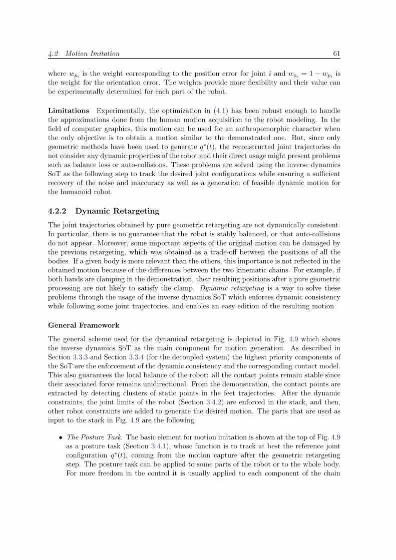
4.2 Motion Imitation 61
where wpi is the weight corresponding to the position error for joint i and woi = 1 − wpi isthe weight for the orientation error. The weights provide more flexibility and their value canbe experimentally determined for each part of the robot.
Limitations Experimentally, the optimization in (4.1) has been robust enough to handlethe approximations done from the human motion acquisition to the robot modeling. In thefield of computer graphics, this motion can be used for an anthropomorphic character whenthe only objective is to obtain a motion similar to the demonstrated one. But, since onlygeometric methods have been used to generate q∗(t), the reconstructed joint trajectories donot consider any dynamic properties of the robot and their direct usage might present problemssuch as balance loss or auto-collisions. These problems are solved using the inverse dynamicsSoT as the following step to track the desired joint configurations while ensuring a sufficientrecovery of the noise and inaccuracy as well as a generation of feasible dynamic motion forthe humanoid robot.
4.2.2 Dynamic Retargeting
The joint trajectories obtained by pure geometric retargeting are not dynamically consistent.In particular, there is no guarantee that the robot is stably balanced, or that auto-collisionsdo not appear. Moreover, some important aspects of the original motion can be damaged bythe previous retargeting, which was obtained as a trade-off between the positions of all thebodies. If a given body is more relevant than the others, this importance is not reflected in theobtained motion because of the differences between the two kinematic chains. For example, ifboth hands are clamping in the demonstration, their resulting positions after a pure geometricprocessing are not likely to satisfy the clamp. Dynamic retargeting is a way to solve theseproblems through the usage of the inverse dynamics SoT which enforces dynamic consistencywhile following some joint trajectories, and enables an easy edition of the resulting motion.
General Framework
The general scheme used for the dynamical retargeting is depicted in Fig. 4.9 which showsthe inverse dynamics SoT as the main component for motion generation. As described inSection 3.3.3 and Section 3.3.4 (for the decoupled system) the highest priority components ofthe SoT are the enforcement of the dynamic consistency and the corresponding contact model.This also guarantees the local balance of the robot: all the contact points remain stable sincetheir associated force remains unidirectional. From the demonstration, the contact points areextracted by detecting clusters of static points in the feet trajectories. After the dynamicconstraints, the joint limits of the robot (Section 3.4.2) are enforced in the stack, and then,other robot constraints are added to generate the desired motion. The parts that are used asinput to the stack in Fig. 4.9 are the following.
• The Posture Task. The basic element for motion imitation is shown at the top of Fig. 4.9as a posture task (Section 3.4.1), whose function is to track at best the reference jointconfiguration q∗(t), coming from the motion capture after the geometric retargetingstep. The posture task can be applied to some parts of the robot or to the whole body.For more freedom in the control it is usually applied to each component of the chain
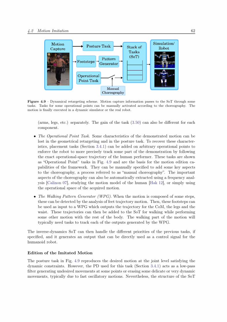
4.2 Motion Imitation 62
Figure 4.9 – Dynamical retargeting scheme. Motion capture information passes to the SoT through sometasks. Tasks for some operational points can be manually activated according to the choreography. Themotion is finally executed in a dynamic simulator or the real robot.
(arms, legs, etc.) separately. The gain of the task (3.50) can also be different for eachcomponent.
• The Operational Point Task. Some characteristics of the demonstrated motion can belost in the geometrical retargeting and in the posture task. To recover these character-istics, placement tasks (Section 3.4.1) can be added on arbitrary operational points toenforce the robot to more precisely track some part of the demonstration by followingthe exact operational-space trajectory of the human performer. These tasks are shownas “Operational Point” tasks in Fig. 4.9 and are the basis for the motion edition ca-pabilities of the framework. They can be manually specified to add some key aspectsto the choreography, a process referred to as “manual choreography”. The importantaspects of the choreography can also be automatically extracted using a frequency anal-ysis [Calinon 07], studying the motion model of the human [Hak 12], or simply usingthe operational space of the acquired motion.
• The Walking Pattern Generator (WPG). When the motion is composed of some steps,these can be detected by the analysis of feet trajectory motion. Then, these footsteps canbe used as input to a WPG which outputs the trajectory for the CoM, the legs and thewaist. These trajectories can then be added to the SoT for walking while performingsome other motion with the rest of the body. The walking part of the motion willtypically need tasks to track each of the outputs generated by the WPG.
The inverse-dynamics SoT can then handle the different priorities of the previous tasks, ifspecified, and it generates an output that can be directly used as a control signal for thehumanoid robot.
Edition of the Imitated Motion
The posture task in Fig. 4.9 reproduces the desired motion at the joint level satisfying thedynamic constraints. However, the PD used for this task (Section 3.4.1) acts as a low-passfilter generating undesired movements at some points or erasing some delicate or very dynamicmovements, typically due to fast oscillatory motions. Nevertheless, the structure of the SoT
4.2 Motion Imitation 63
can be used to overcome these problems by adding operational point tasks, as explainedabove, which can enhance or even modify the original motion. For a given operational pointxi, a selection matrix Sx can be defined to enable and disable the control of some degrees offreedom of SE(3) to give more freedom to the task. For example, if the position is representedby Cartesian coordinates and the orientation by roll, pitch and yaw angles, then xi ∈ R
6 andthe selection matrix is given by
Sx =
s1 0 0 0 0 00 s2 0 0 0 00 0 s3 0 0 00 0 0 s4 0 00 0 0 0 s5 00 0 0 0 0 s6
(4.3)
where sj is a binary element whose value can be either 1 or 0. If it is 1, that particular elementof the pose will be controlled, and if it is 0, the corresponding element will be unconstrainedand its motion will be a result of the whole body dynamics. In general, the motion obtainedwith the posture task can be edited with the operational point task in two ways.
• Specification of target points. A new desired target for a chosen operational point canbe specified without defining the desired trajectory to reach it. This point can bedetermined using forward kinematics on an operational point to compute its positionfrom the geometric retargeting, or it can be arbitrarily set.
• Specification of a trajectory. Let the trajectory for the operational point x be calledxo(t). The new trajectory that will be set as the desired trajectory for the operationalpoint will be xn(t) = xo(t)+xm(t), where xm(t) is the trajectory modification that canbe done on any of the six degrees of freedom of x. This trajectory modification xm(t)can be time varying or constant, according to the requirements.
It is important to point out that the operational task must have higher priority than theposture task it would interfere with. For instance, if an operational task is added to the hand,the priority of the arm posture task must be reduced. Alternatively, the task can be removed,but it is preferred to be kept, as it will serve as a “guide” for the new trajectory. If thesepriority considerations are not taken into account, the desired motion would be blinded bythe solutions satisfying the posture task with higher priority, and the desired effect would notbe achieved. Additional tasks, such as a task for the gaze, can also be added to modify theoriginal motion.
4.2.3 Experimental Setup
A motion capture system, which provides the spatial trajectory for each of the markers thatare distributed on the human body, is used to acquire the motion performed by a humandemonstrator. The markers are located in characteristic parts of the body, as Fig. 4.10 shows[H. 11], in order to minimize the motion of the skin with respect to the bones, and to facilitatetheir temporal tracking. For example, they must be placed as close as possible to the centerof the articulations to avoid undesired translations when joints rotate, and the configurationshould not be symmetric so that the temporal tracking of the markers is not perturbed. If

4.2 Motion Imitation 64
Figure 4.10 – Position of the markers in the human body and calibration position
Figure 4.11 – Skeleton showing the rigid bodies and the markers associated to them
there is symmetry, some ambiguity might appear leading to problems in markers identification.Due to this reason, in Fig. 4.10 a small plank is used at each wrist so that the three markerslocated at the hand do not form an equilateral triangle and are easier to track. In this work,35 markers were used.
Skeleton The markers are then manually associated to form a skeleton which is composedof a hierarchy of rigid bodies in the form of a tree. These rigid bodies are sometimes referredto as links or bones of the skeleton and each of them has a frame that is defined by threemarkers. The skeleton used in this work, shown in Figure 4.11, consists of 15 rigid bodies andis the one proposed in [H. 11]. It should be noted that only after the skeleton is generated,the position and orientation of the rigid bodies composing it can be obtained.
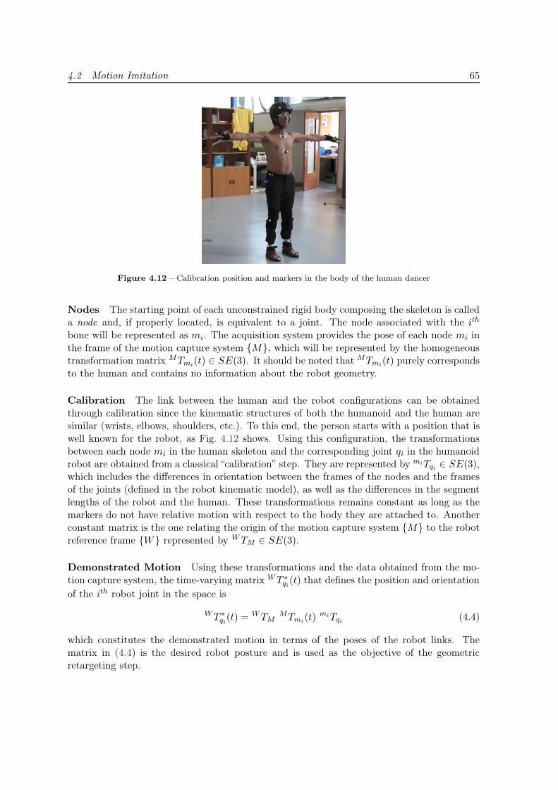
4.2 Motion Imitation 65
Figure 4.12 – Calibration position and markers in the body of the human dancer
Nodes The starting point of each unconstrained rigid body composing the skeleton is calleda node and, if properly located, is equivalent to a joint. The node associated with the ith
bone will be represented as mi. The acquisition system provides the pose of each node mi inthe frame of the motion capture system {M}, which will be represented by the homogeneoustransformation matrix MTmi
(t) ∈ SE(3). It should be noted that MTmi(t) purely corresponds
to the human and contains no information about the robot geometry.
Calibration The link between the human and the robot configurations can be obtainedthrough calibration since the kinematic structures of both the humanoid and the human aresimilar (wrists, elbows, shoulders, etc.). To this end, the person starts with a position that iswell known for the robot, as Fig. 4.12 shows. Using this configuration, the transformationsbetween each node mi in the human skeleton and the corresponding joint qi in the humanoidrobot are obtained from a classical “calibration” step. They are represented by miTqi ∈ SE(3),which includes the differences in orientation between the frames of the nodes and the framesof the joints (defined in the robot kinematic model), as well as the differences in the segmentlengths of the robot and the human. These transformations remains constant as long as themarkers do not have relative motion with respect to the body they are attached to. Anotherconstant matrix is the one relating the origin of the motion capture system {M} to the robotreference frame {W} represented by WTM ∈ SE(3).
Demonstrated Motion Using these transformations and the data obtained from the mo-tion capture system, the time-varying matrix WT ∗
qi(t) that defines the position and orientation
of the ith robot joint in the space is
WT ∗qi(t) = WTM
MTmi(t) miTqi (4.4)
which constitutes the demonstrated motion in terms of the poses of the robot links. Thematrix in (4.4) is the desired robot posture and is used as the objective of the geometricretargeting step.
4.2 Motion Imitation 66
Motion Capture System For this particular experience, the human motion was acquiredusing the Motion Analysis (http://www.motionanalysis.com/) motion capture system con-sisting of ten infrared cameras distributed around the experimentation zone and calibratedby the Motion Analysis software. The acquisition frequency was 200 Hz with a precision of 2mm of nearly pure white noise and negligible bias. More than thirty minutes of motions werecaptured. The captured data for the most important movements used in this work is freelyavailable3 along with the corresponding geometric retargeting and the results of the dynamicretargeting that uses the inverse-dynamics approach, explained in Sections 4.2.1 and 4.2.2.
4.2.4 Robot Dancing Simulation
The motion of a person performing a pop dance was acquired using the motion capture system,as Fig. 4.13a shows. During this motion the dancer keeps the feet almost at the same positionand most of the movement is done by the upper body and the legs. The acquired motion wasretargeted to a modified HRP-2 model, and it was edited to correct the retargeting error andto introduce new undemonstrated features. The model of HRP-2 was modified by adding oneextra degree of freedom both at the chest and the neck joints with the purpose of obtaining amodel closer to the human body and more suitable for the dance imitation. The kinematicalstructure thus obtained contains 32 DoF and resembles more the structure of HRP-4 thanthat of HRP-2. For this reason, these results have only been implemented in simulation.
The initial trajectory for the joints is obtained from the captured motion using the ge-ometric retargeting, but it is neither stable nor dynamically consistent as Fig. 4.13b shows.Then, the dynamic retargeting is applied keeping both feet in contact with the ground at allmoments but only the posture task is added to the SoT to track the joint trajectories; theresults are shown in Fig. 4.13c. The obtained motion is stable but some problems appearlike an auto-collision between the right hand and the head shown in the fourth thumbnail.Also, the geometric and dynamic retargetting have lost some data and produced some errorscompared to the initial demonstrated trajectory. For this particular motion, three editionswere applied:
• The right hand motion was corrected to avoid auto-collisions.
• The knee oscillations (smoothed by the PD in (3.50)) were enhanced.
• An additional motion of the left foot (sliding), not present in the initial demonstration,was introduced.
The sequence of tasks showing the instants of time when these modifications were added ispresented in Fig. 4.14 and the final motion is shown in Fig. 4.13d. More details about thesethree editions are provided below.
Right hand motion
The fast up and down motion of the dancer’s right arm was smoothed as a consequence of thePD used in the task that tracks the joints. This was especially noted when the arm could notreach the upper positions that the dancer performed. To correct this effect, an operationaltask to raise more the arm was introduced. The result is shown in Fig. 4.15.
3http://projects.laas.fr/gepetto/novela/noveladb
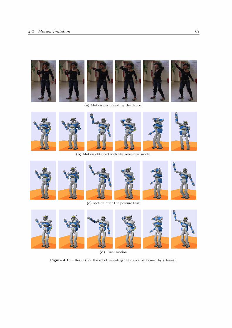
4.2 Motion Imitation 67
(a) Motion performed by the dancer
(b) Motion obtained with the geometric model
(c) Motion after the posture task
(d) Final motion
Figure 4.13 – Results for the robot imitating the dance performed by a human.
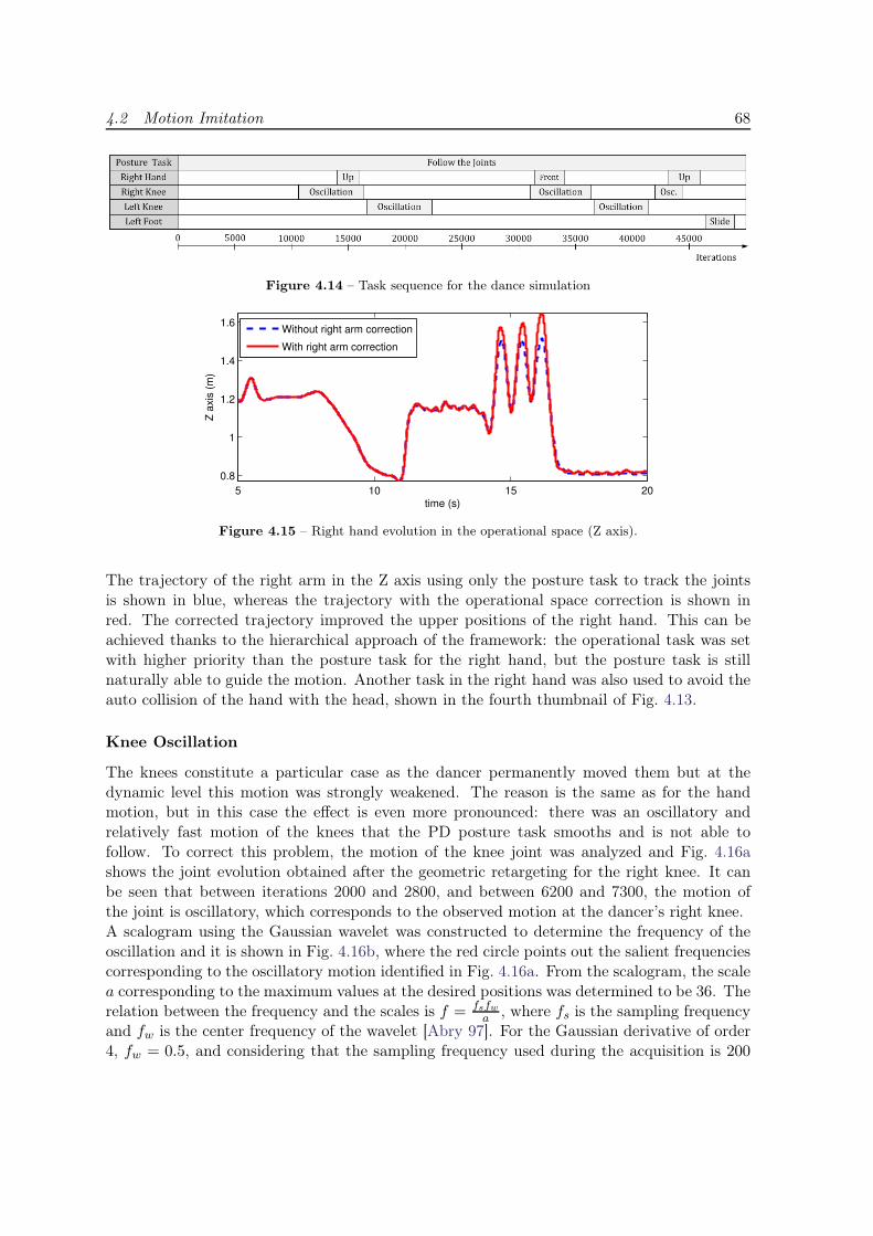
4.2 Motion Imitation 68
Figure 4.14 – Task sequence for the dance simulation
5 10 15 20
0.8
1
1.2
1.4
1.6
time (s)
Z a
xis
(m
)
Without right arm correction
With right arm correction
Figure 4.15 – Right hand evolution in the operational space (Z axis).
The trajectory of the right arm in the Z axis using only the posture task to track the jointsis shown in blue, whereas the trajectory with the operational space correction is shown inred. The corrected trajectory improved the upper positions of the right hand. This can beachieved thanks to the hierarchical approach of the framework: the operational task was setwith higher priority than the posture task for the right hand, but the posture task is stillnaturally able to guide the motion. Another task in the right hand was also used to avoid theauto collision of the hand with the head, shown in the fourth thumbnail of Fig. 4.13.
Knee Oscillation
The knees constitute a particular case as the dancer permanently moved them but at thedynamic level this motion was strongly weakened. The reason is the same as for the handmotion, but in this case the effect is even more pronounced: there was an oscillatory andrelatively fast motion of the knees that the PD posture task smooths and is not able tofollow. To correct this problem, the motion of the knee joint was analyzed and Fig. 4.16ashows the joint evolution obtained after the geometric retargeting for the right knee. It canbe seen that between iterations 2000 and 2800, and between 6200 and 7300, the motion ofthe joint is oscillatory, which corresponds to the observed motion at the dancer’s right knee.A scalogram using the Gaussian wavelet was constructed to determine the frequency of theoscillation and it is shown in Fig. 4.16b, where the red circle points out the salient frequenciescorresponding to the oscillatory motion identified in Fig. 4.16a. From the scalogram, the scalea corresponding to the maximum values at the desired positions was determined to be 36. Therelation between the frequency and the scales is f = fsfw
a, where fs is the sampling frequency
and fw is the center frequency of the wavelet [Abry 97]. For the Gaussian derivative of order4, fw = 0.5, and considering that the sampling frequency used during the acquisition is 200
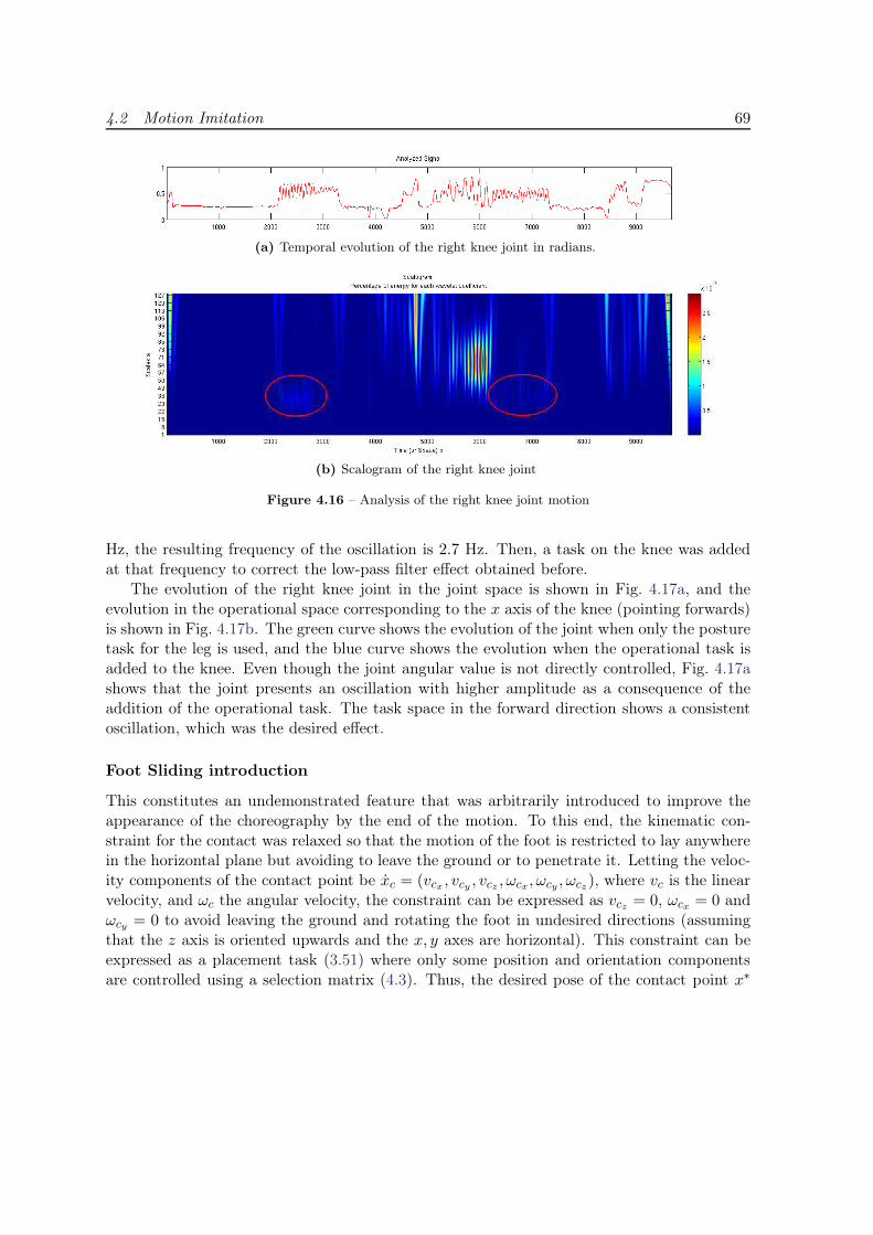
4.2 Motion Imitation 69
(a) Temporal evolution of the right knee joint in radians.
(b) Scalogram of the right knee joint
Figure 4.16 – Analysis of the right knee joint motion
Hz, the resulting frequency of the oscillation is 2.7 Hz. Then, a task on the knee was addedat that frequency to correct the low-pass filter effect obtained before.
The evolution of the right knee joint in the joint space is shown in Fig. 4.17a, and theevolution in the operational space corresponding to the x axis of the knee (pointing forwards)is shown in Fig. 4.17b. The green curve shows the evolution of the joint when only the posturetask for the leg is used, and the blue curve shows the evolution when the operational task isadded to the knee. Even though the joint angular value is not directly controlled, Fig. 4.17ashows that the joint presents an oscillation with higher amplitude as a consequence of theaddition of the operational task. The task space in the forward direction shows a consistentoscillation, which was the desired effect.
Foot Sliding introduction
This constitutes an undemonstrated feature that was arbitrarily introduced to improve theappearance of the choreography by the end of the motion. To this end, the kinematic con-straint for the contact was relaxed so that the motion of the foot is restricted to lay anywherein the horizontal plane but avoiding to leave the ground or to penetrate it. Letting the veloc-ity components of the contact point be xc = (vcx , vcy , vcz , ωcx, ωcy , ωcz), where vc is the linearvelocity, and ωc the angular velocity, the constraint can be expressed as vcz = 0, ωcx = 0 andωcy = 0 to avoid leaving the ground and rotating the foot in undesired directions (assumingthat the z axis is oriented upwards and the x, y axes are horizontal). This constraint can beexpressed as a placement task (3.51) where only some position and orientation componentsare controlled using a selection matrix (4.3). Thus, the desired pose of the contact point x∗
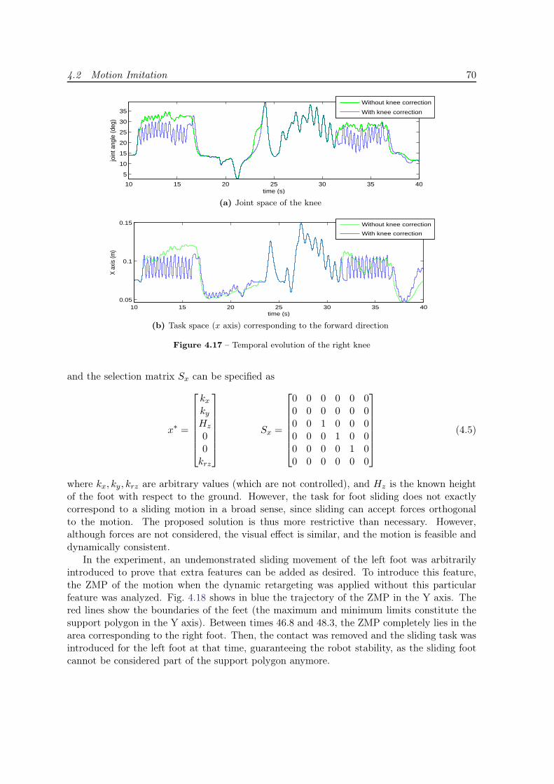
4.2 Motion Imitation 70
10 15 20 25 30 35 40
5
10
15
20
25
30
35
time (s)
join
t ang
le (d
eg)
Without knee correction
With knee correction
(a) Joint space of the knee
10 15 20 25 30 35 400.05
0.1
0.15
time (s)
X ax
is (m
)
Without knee correction
With knee correction
(b) Task space (x axis) corresponding to the forward direction
Figure 4.17 – Temporal evolution of the right knee
and the selection matrix Sx can be specified as
x∗ =
kxkyHz
00krz
Sx =
0 0 0 0 0 00 0 0 0 0 00 0 1 0 0 00 0 0 1 0 00 0 0 0 1 00 0 0 0 0 0
(4.5)
where kx, ky , krz are arbitrary values (which are not controlled), and Hz is the known heightof the foot with respect to the ground. However, the task for foot sliding does not exactlycorrespond to a sliding motion in a broad sense, since sliding can accept forces orthogonalto the motion. The proposed solution is thus more restrictive than necessary. However,although forces are not considered, the visual effect is similar, and the motion is feasible anddynamically consistent.
In the experiment, an undemonstrated sliding movement of the left foot was arbitrarilyintroduced to prove that extra features can be added as desired. To introduce this feature,the ZMP of the motion when the dynamic retargeting was applied without this particularfeature was analyzed. Fig. 4.18 shows in blue the trajectory of the ZMP in the Y axis. Thered lines show the boundaries of the feet (the maximum and minimum limits constitute thesupport polygon in the Y axis). Between times 46.8 and 48.3, the ZMP completely lies in thearea corresponding to the right foot. Then, the contact was removed and the sliding task wasintroduced for the left foot at that time, guaranteeing the robot stability, as the sliding footcannot be considered part of the support polygon anymore.
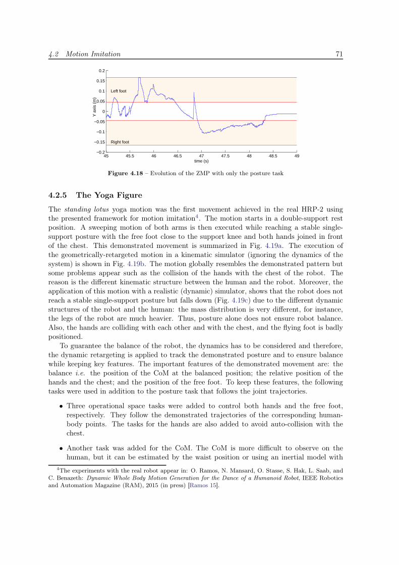
4.2 Motion Imitation 71
45 45.5 46 46.5 47 47.5 48 48.5 49−0.2
−0.15
−0.1
−0.05
0
0.05
0.1
0.15
0.2
Left foot
Right foot
time (s)
Y a
xis
(m)
Figure 4.18 – Evolution of the ZMP with only the posture task
4.2.5 The Yoga Figure
The standing lotus yoga motion was the first movement achieved in the real HRP-2 usingthe presented framework for motion imitation4. The motion starts in a double-support restposition. A sweeping motion of both arms is then executed while reaching a stable single-support posture with the free foot close to the support knee and both hands joined in frontof the chest. This demonstrated movement is summarized in Fig. 4.19a. The execution ofthe geometrically-retargeted motion in a kinematic simulator (ignoring the dynamics of thesystem) is shown in Fig. 4.19b. The motion globally resembles the demonstrated pattern butsome problems appear such as the collision of the hands with the chest of the robot. Thereason is the different kinematic structure between the human and the robot. Moreover, theapplication of this motion with a realistic (dynamic) simulator, shows that the robot does notreach a stable single-support posture but falls down (Fig. 4.19c) due to the different dynamicstructures of the robot and the human: the mass distribution is very different, for instance,the legs of the robot are much heavier. Thus, posture alone does not ensure robot balance.Also, the hands are colliding with each other and with the chest, and the flying foot is badlypositioned.
To guarantee the balance of the robot, the dynamics has to be considered and therefore,the dynamic retargeting is applied to track the demonstrated posture and to ensure balancewhile keeping key features. The important features of the demonstrated movement are: thebalance i.e. the position of the CoM at the balanced position; the relative position of thehands and the chest; and the position of the free foot. To keep these features, the followingtasks were used in addition to the posture task that follows the joint trajectories.
• Three operational space tasks were added to control both hands and the free foot,respectively. They follow the demonstrated trajectories of the corresponding human-body points. The tasks for the hands are also added to avoid auto-collision with thechest.
• Another task was added for the CoM. The CoM is more difficult to observe on thehuman, but it can be estimated by the waist position or using an inertial model with
4The experiments with the real robot appear in: O. Ramos, N. Mansard, O. Stasse, S. Hak, L. Saab, andC. Benazeth: Dynamic Whole Body Motion Generation for the Dance of a Humanoid Robot, IEEE Roboticsand Automation Magazine (RAM), 2015 (in press) [Ramos 15].
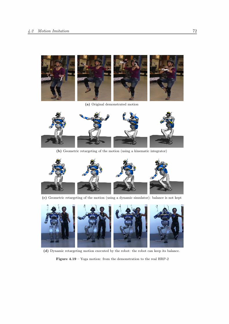
4.2 Motion Imitation 72
(a) Original demonstrated motion
(b) Geometric retargeting of the motion (using a kinematic integrator)
(c) Geometric retargeting of the motion (using a dynamic simulator): balance is not kept
(d) Dynamic retargeting motion executed by the robot: the robot can keep its balance.
Figure 4.19 – Yoga motion: from the demonstration to the real HRP-2

4.2 Motion Imitation 73
(a) (b) (c) (d)
Figure 4.20 – Motion acquisition of a human dancer
the correct mass distribution. However, even if the human CoM is recovered, it cannotbe guaranteed that it generates stable motions in the robot due to the mass difference.Thus, an artificial pattern for the CoM was imposed to enforce balance since CoMaccelerations might destabilize the robot and the approach cannot predict those states.The pattern specifies that the CoM lies inside the support polygon and is obtained byexperimentally determining the timings for the change in the supports of the humanperformer.
The SoT is finally composed of the dynamics and contact constraints, a task tracking theCoM artificial pattern, a task tracking the demonstrated right hand, left hand and right foot,and a task tracking the geometrically-retargeted configuration. The task tracking the freefoot is added only when the foot leaves the ground. The motion executed by the robot isshown in Fig. 4.19d.
4.2.6 Long-sequence Motion Generation
The same generic task sequence described above and used for the yoga movement can be ap-plied to treat several motion sequences automatically. In particular, the motion correspondingto a long choreography performed by a hip-hop dancer was acquired. Fig. 4.20 shows sometypical patterns of the movements demonstrated by the human dancer (with the markers onhis body) in the motion capture acquisition room: motion in double support (Fig 4.20a andFig. 4.20b), motion in single support (Fig. 4.20c), and motion of the upper body while walking(Fig. 4.20d). In this acquisition, the small plank for the hand (Section 4.2.3) was not usedsince the demonstrator’s hands were big enough to properly locate the markers avoiding theundesired acquisition symmetries.From the choreography performed by the human, a choreography was designed for HRP-2.This choreography was presented in October 2012 in a live demonstration in front of morethan 1000 people in the city of Toulouse. The demonstration consisted in both the robot andthe human performing the movements side by side as Fig 4.21 shows.Three of the typical execution patterns performed in the demonstration, consisting in doublesupport motion, single support motion, and motion while walking, are detailed below.
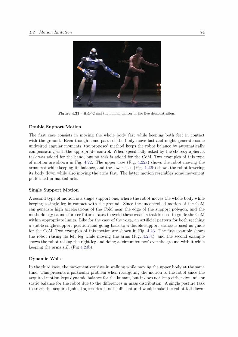
4.2 Motion Imitation 74
Figure 4.21 – HRP-2 and the human dancer in the live demonstration.
Double Support Motion
The first case consists in moving the whole body fast while keeping both feet in contactwith the ground. Even though some parts of the body move fast and might generate someundesired angular moments, the proposed method keeps the robot balance by automaticallycompensating with the appropriate control. When specifically asked by the choreographer, atask was added for the hand, but no task is added for the CoM. Two examples of this typeof motion are shown in Fig. 4.22. The upper case (Fig. 4.22a) shows the robot moving thearms fast while keeping its balance, and the lower case (Fig. 4.22b) shows the robot loweringits body down while also moving the arms fast. The latter motion resembles some movementperformed in martial arts.
Single Support Motion
A second type of motion is a single support one, where the robot moves the whole body whilekeeping a single leg in contact with the ground. Since the uncontrolled motion of the CoMcan generate high accelerations of the CoM near the edge of the support polygon, and themethodology cannot foresee future states to avoid these cases, a task is used to guide the CoMwithin appropriate limits. Like for the case of the yoga, an artificial pattern for both reachinga stable single-support position and going back to a double-support stance is used as guidefor the CoM. Two examples of this motion are shown in Fig. 4.23. The first example showsthe robot raising its left leg while moving the arms (Fig. 4.23a), and the second exampleshows the robot raising the right leg and doing a ‘circumference’ over the ground with it whilekeeping the arms still (Fig 4.23b).
Dynamic Walk
In the third case, the movement consists in walking while moving the upper body at the sametime. This presents a particular problem when retargeting the motion to the robot since theacquired motion kept dynamic balance for the human, but it does not keep either dynamic orstatic balance for the robot due to the differences in mass distribution. A single posture taskto track the acquired joint trajectories is not sufficient and would make the robot fall down.
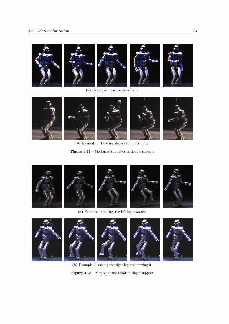
4.2 Motion Imitation 75
(a) Example 1: fast arms motion
(b) Example 2: lowering down the upper body
Figure 4.22 – Motion of the robot in double support
(a) Example 1: raising the left leg upwards
(b) Example 2: raising the right leg and moving it
Figure 4.23 – Motion of the robot in single support
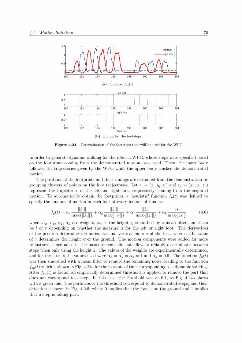
4.2 Motion Imitation 76
190 192 194 196 198 200 202 204
0
0.5
1
1.5
left foot
right foot
(a) Function fsp(t).
190 192 194 196 198 200 202 2040
0.5
1left foot
190 192 194 196 198 200 202 2040
0.5
1
time (s)
right foot
(b) Timing for the footsteps
Figure 4.24 – Determination of the footsteps that will be used for the WPG
In order to generate dynamic walking for the robot a WPG, whose steps were specified basedon the footprints coming from the demonstrated motion, was used. Then, the lower bodyfollowed the trajectories given by the WPG while the upper body tracked the demonstratedmotion.
The positions of the footprints and their timings are extracted from the demonstration bygrouping clusters of points on the foot trajectories. Let r
l= (x
l, y
l, z
l) and rr = (xr, yr, zr)
represent the trajectories of the left and right foot, respectively, coming from the acquiredmotion. To automatically obtain the footprints, a ‘heuristic’ function fp(t) was defined tospecify the amount of motion in each foot at every instant of time as:
fp(t) = αx‖xi‖
max{‖xi‖}+ αy
‖yi‖max{‖yi‖}
+ αz‖zi‖
max{‖zi‖}+ αh
zsimax{zsi}
(4.6)
where αx, αy, αz, αh are weights, zsi is the height zi smoothed by a mean filter, and i canbe l or r depending on whether the measure is for the left or right foot. The derivativesof the position determine the horizontal and vertical motion of the feet, whereas the valueof z determines the height over the ground. The motion components were added for morerobustness, since noise in the measurements did not allow to reliably discriminate betweensteps when only using the height z. The values of the weights are experimentally determined,and for these tests the values used were αx = αy = αz = 1 and αh = 0.5. The function fp(t)was then smoothed with a mean filter to remove the remaining noise, leading to the functionfsp(t) which is shown in Fig. 4.24a for the instants of time corresponding to a dynamic walking.After fsp(t) is found, an empirically determined threshold is applied to remove the part thatdoes not correspond to a step. In this case, the threshold was at 0.1, as Fig. 4.24a showswith a green line. The parts above the threshold correspond to demonstrated steps, and theirdetection is shown in Fig. 4.24b where 0 implies that the foot is on the ground and 1 impliesthat a step is taking part.

4.2 Motion Imitation 77
(a) Frontal view
(b) Lateral view
Figure 4.25 – Walking while arbitrarily moving the upper part of the body
The footprints are then used as input to a WPG [Kajita 03a] to compute a walkingtrajectory for both the feet and the CoM. The CoM task is added as the top-priority task,while a task is added to drive the position of the flying foot during each step. The posture taskis added for the upper body and additional tasks are eventually added to improve the handor the head placements depending on the choreography. The hands produce an importantmomentum, especially when the choreography imposes some movements that are contrary tothe natural walking motion. The momentum is however corrected by the whole-body inverse-dynamics scheme and does not disturb the balance. Fig. 4.25 shows an example of this typeof motion. It can be observed that the robot walks dynamically while moving its arms witharbitrary motion that follows the demonstrated movements.
The captured and experimental joint trajectories for two typical joints (at the shoulders) isshown in Fig. 4.26. It can be noticed that the trajectories obtained with the dynamic controlfollow closely the desired ones, but the control also acts as a ‘low pass filter’. This attenuationcan be controlled by changing the gain of the task. If the gain is larger, the joints move fasterand the trajectory is closer to the desired one. However, the gain cannot be arbitrarily bigsince it is eventually limited by the mechanical constraints of the robot such as the maximumvelocity of the joints.
4.2.7 Conclusion
The methodology presented for imitation allows to quickly and efficiently generate long se-quence of dynamic movements for a humanoid robot. The motion generation is based on acombination of two very efficient tools: the motion capture, and the hierarchized operational-space inverse-dynamics, which enables the retargeted dynamics to fit with the constraints of
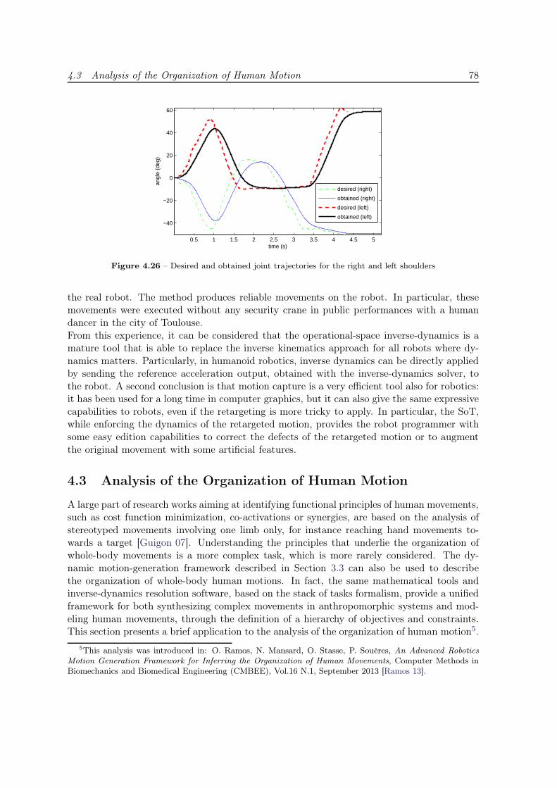
4.3 Analysis of the Organization of Human Motion 78
0.5 1 1.5 2 2.5 3 3.5 4 4.5 5
−40
−20
0
20
40
60
time (s)
angl
e (d
eg)
desired (right)
obtained (right)
desired (left)
obtained (left)
Figure 4.26 – Desired and obtained joint trajectories for the right and left shoulders
the real robot. The method produces reliable movements on the robot. In particular, thesemovements were executed without any security crane in public performances with a humandancer in the city of Toulouse.From this experience, it can be considered that the operational-space inverse-dynamics is amature tool that is able to replace the inverse kinematics approach for all robots where dy-namics matters. Particularly, in humanoid robotics, inverse dynamics can be directly appliedby sending the reference acceleration output, obtained with the inverse-dynamics solver, tothe robot. A second conclusion is that motion capture is a very efficient tool also for robotics:it has been used for a long time in computer graphics, but it can also give the same expressivecapabilities to robots, even if the retargeting is more tricky to apply. In particular, the SoT,while enforcing the dynamics of the retargeted motion, provides the robot programmer withsome easy edition capabilities to correct the defects of the retargeted motion or to augmentthe original movement with some artificial features.
4.3 Analysis of the Organization of Human Motion
A large part of research works aiming at identifying functional principles of human movements,such as cost function minimization, co-activations or synergies, are based on the analysis ofstereotyped movements involving one limb only, for instance reaching hand movements to-wards a target [Guigon 07]. Understanding the principles that underlie the organization ofwhole-body movements is a more complex task, which is more rarely considered. The dy-namic motion-generation framework described in Section 3.3 can also be used to describethe organization of whole-body human motions. In fact, the same mathematical tools andinverse-dynamics resolution software, based on the stack of tasks formalism, provide a unifiedframework for both synthesizing complex movements in anthropomorphic systems and mod-eling human movements, through the definition of a hierarchy of objectives and constraints.This section presents a brief application to the analysis of the organization of human motion5.
5This analysis was introduced in: O. Ramos, N. Mansard, O. Stasse, P. Souères, An Advanced RoboticsMotion Generation Framework for Inferring the Organization of Human Movements, Computer Methods inBiomechanics and Biomedical Engineering (CMBEE), Vol.16 N.1, September 2013 [Ramos 13].
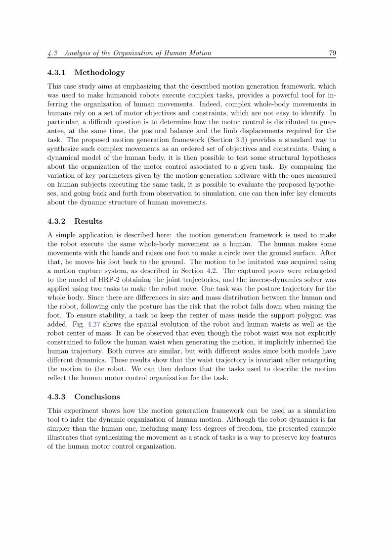
4.3 Analysis of the Organization of Human Motion 79
4.3.1 Methodology
This case study aims at emphasizing that the described motion generation framework, whichwas used to make humanoid robots execute complex tasks, provides a powerful tool for in-ferring the organization of human movements. Indeed, complex whole-body movements inhumans rely on a set of motor objectives and constraints, which are not easy to identify. Inparticular, a difficult question is to determine how the motor control is distributed to guar-antee, at the same time, the postural balance and the limb displacements required for thetask. The proposed motion generation framework (Section 3.3) provides a standard way tosynthesize such complex movements as an ordered set of objectives and constraints. Using adynamical model of the human body, it is then possible to test some structural hypothesesabout the organization of the motor control associated to a given task. By comparing thevariation of key parameters given by the motion generation software with the ones measuredon human subjects executing the same task, it is possible to evaluate the proposed hypothe-ses, and going back and forth from observation to simulation, one can then infer key elementsabout the dynamic structure of human movements.
4.3.2 Results
A simple application is described here: the motion generation framework is used to makethe robot execute the same whole-body movement as a human. The human makes somemovements with the hands and raises one foot to make a circle over the ground surface. Afterthat, he moves his foot back to the ground. The motion to be imitated was acquired usinga motion capture system, as described in Section 4.2. The captured poses were retargetedto the model of HRP-2 obtaining the joint trajectories, and the inverse-dynamics solver wasapplied using two tasks to make the robot move. One task was the posture trajectory for thewhole body. Since there are differences in size and mass distribution between the human andthe robot, following only the posture has the risk that the robot falls down when raising thefoot. To ensure stability, a task to keep the center of mass inside the support polygon wasadded. Fig. 4.27 shows the spatial evolution of the robot and human waists as well as therobot center of mass. It can be observed that even though the robot waist was not explicitlyconstrained to follow the human waist when generating the motion, it implicitly inherited thehuman trajectory. Both curves are similar, but with different scales since both models havedifferent dynamics. These results show that the waist trajectory is invariant after retargetingthe motion to the robot. We can then deduce that the tasks used to describe the motionreflect the human motor control organization for the task.
4.3.3 Conclusions
This experiment shows how the motion generation framework can be used as a simulationtool to infer the dynamic organization of human motion. Although the robot dynamics is farsimpler than the human one, including many less degrees of freedom, the presented exampleillustrates that synthesizing the movement as a stack of tasks is a way to preserve key featuresof the human motor control organization.
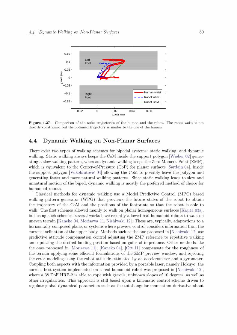
4.4 Dynamic Walking on Non-Planar Surfaces 80
−0.02 0 0.02 0.04 0.06
−0.15
−0.1
−0.05
0
0.05
0.1
0.15
LeftFoot
Right Foot
x axis (m)
y ax
is (
m)
Human waist
Robot waist
Robot CoM
Figure 4.27 – Comparison of the waist trajectories of the human and the robot. The robot waist is notdirectly constrained but the obtained trajectory is similar to the one of the human.
4.4 Dynamic Walking on Non-Planar Surfaces
There exist two types of walking schemes for bipedal systems: static walking, and dynamicwalking. Static walking always keeps the CoM inside the support polygon [Wieber 02] gener-ating a slow walking pattern, whereas dynamic walking keeps the Zero Moment Point (ZMP),which is equivalent to the Center-of-Pressure (CoP) for planar surfaces [Sardain 04], insidethe support polygon [Vukobratović 04] allowing the CoM to possibly leave the polygon andgenerating faster and more natural walking patterns. Since static walking leads to slow andunnatural motion of the biped, dynamic walking is mostly the preferred method of choice forhumanoid robots.
Classical methods for dynamic walking use a Model Predictive Control (MPC) basedwalking pattern generator (WPG) that previews the future states of the robot to obtainthe trajectory of the CoM and the positions of the footprints so that the robot is able towalk. The first schemes allowed mainly to walk on planar homogeneous surfaces [Kajita 03a],but using such schemes, several works have recently allowed real humanoid robots to walk onuneven terrain [Kaneko 04, Morisawa 11, Nishiwaki 12]. These are, typically, adaptations to ahorizontally composed plane, or systems where preview control considers information from thecurrent inclination of the upper body. Methods such as the one proposed in [Nishiwaki 12] usepredictive attitude compensation control adjusting the ZMP reference to repetitive walkingand updating the desired landing position based on gains of impedance. Other methods likethe ones proposed in [Morisawa 11], [Kaneko 04], [Ott 11] compensate for the roughness ofthe terrain applying some efficient formulations of the ZMP preview window, and rejectingthe error modeling using the robot attitude estimated by an accelerometer and a gyrometer.Coupling both aspects with the information provided by a portable laser, namely Hokuyo, thecurrent best system implemented on a real humanoid robot was proposed in [Nishiwaki 12],where a 38 DoF HRP-2 is able to cope with gravels, unknown slopes of 10 degrees, as well asother irregularities. This approach is still based upon a kinematic control scheme driven toregulate global dynamical parameters such as the total angular momentum derivative about
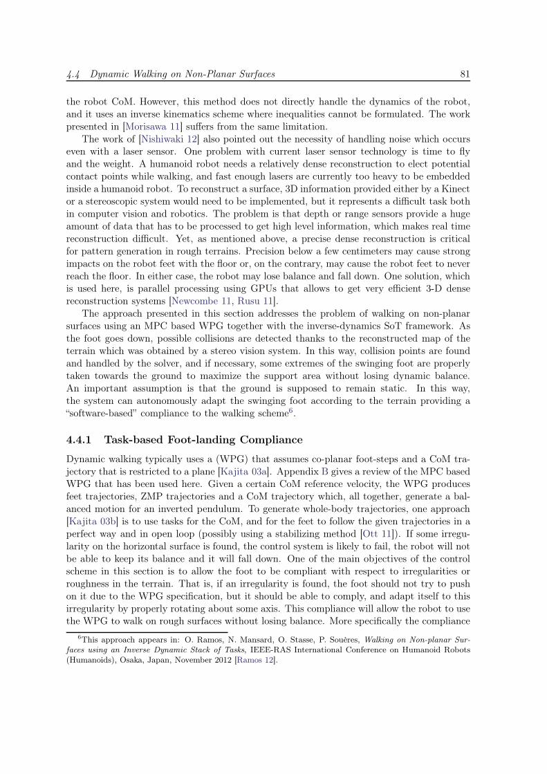
4.4 Dynamic Walking on Non-Planar Surfaces 81
the robot CoM. However, this method does not directly handle the dynamics of the robot,and it uses an inverse kinematics scheme where inequalities cannot be formulated. The workpresented in [Morisawa 11] suffers from the same limitation.
The work of [Nishiwaki 12] also pointed out the necessity of handling noise which occurseven with a laser sensor. One problem with current laser sensor technology is time to flyand the weight. A humanoid robot needs a relatively dense reconstruction to elect potentialcontact points while walking, and fast enough lasers are currently too heavy to be embeddedinside a humanoid robot. To reconstruct a surface, 3D information provided either by a Kinector a stereoscopic system would need to be implemented, but it represents a difficult task bothin computer vision and robotics. The problem is that depth or range sensors provide a hugeamount of data that has to be processed to get high level information, which makes real timereconstruction difficult. Yet, as mentioned above, a precise dense reconstruction is criticalfor pattern generation in rough terrains. Precision below a few centimeters may cause strongimpacts on the robot feet with the floor or, on the contrary, may cause the robot feet to neverreach the floor. In either case, the robot may lose balance and fall down. One solution, whichis used here, is parallel processing using GPUs that allows to get very efficient 3-D densereconstruction systems [Newcombe 11, Rusu 11].
The approach presented in this section addresses the problem of walking on non-planarsurfaces using an MPC based WPG together with the inverse-dynamics SoT framework. Asthe foot goes down, possible collisions are detected thanks to the reconstructed map of theterrain which was obtained by a stereo vision system. In this way, collision points are foundand handled by the solver, and if necessary, some extremes of the swinging foot are properlytaken towards the ground to maximize the support area without losing dynamic balance.An important assumption is that the ground is supposed to remain static. In this way,the system can autonomously adapt the swinging foot according to the terrain providing a“software-based” compliance to the walking scheme6.
4.4.1 Task-based Foot-landing Compliance
Dynamic walking typically uses a (WPG) that assumes co-planar foot-steps and a CoM tra-jectory that is restricted to a plane [Kajita 03a]. Appendix B gives a review of the MPC basedWPG that has been used here. Given a certain CoM reference velocity, the WPG producesfeet trajectories, ZMP trajectories and a CoM trajectory which, all together, generate a bal-anced motion for an inverted pendulum. To generate whole-body trajectories, one approach[Kajita 03b] is to use tasks for the CoM, and for the feet to follow the given trajectories in aperfect way and in open loop (possibly using a stabilizing method [Ott 11]). If some irregu-larity on the horizontal surface is found, the control system is likely to fail, the robot will notbe able to keep its balance and it will fall down. One of the main objectives of the controlscheme in this section is to allow the foot to be compliant with respect to irregularities orroughness in the terrain. That is, if an irregularity is found, the foot should not try to pushon it due to the WPG specification, but it should be able to comply, and adapt itself to thisirregularity by properly rotating about some axis. This compliance will allow the robot to usethe WPG to walk on rough surfaces without losing balance. More specifically the compliance
6This approach appears in: O. Ramos, N. Mansard, O. Stasse, P. Souères, Walking on Non-planar Sur-faces using an Inverse Dynamic Stack of Tasks, IEEE-RAS International Conference on Humanoid Robots(Humanoids), Osaka, Japan, November 2012 [Ramos 12].
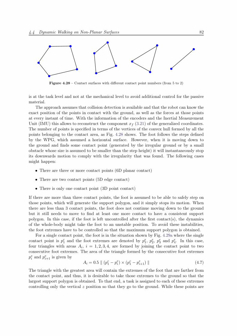
4.4 Dynamic Walking on Non-Planar Surfaces 82
Figure 4.28 – Contact surfaces with different contact point numbers (from 5 to 2)
is at the task level and not at the mechanical level to avoid additional control for the passivematerial.
The approach assumes that collision detection is available and that the robot can know theexact position of the points in contact with the ground, as well as the forces at those pointsat every instant of time. With the information of the encoders and the Inertial MeasurementUnit (IMU) this allows to reconstruct the component xf (3.21) of the generalized coordinates.The number of points is specified in terms of the vertices of the convex hull formed by all thepoints belonging to the contact area, as Fig. 4.28 shows. The foot follows the steps definedby the WPG, which assumed a horizontal surface. However, when it is moving down tothe ground and finds some contact point (generated by the irregular ground or by a smallobstacle whose size is assumed to be smaller than the step height) it will instantaneously stopits downwards motion to comply with the irregularity that was found. The following casesmight happen:
• There are three or more contact points (6D planar contact)
• There are two contact points (5D edge contact)
• There is only one contact point (3D point contact)
If there are more than three contact points, the foot is assumed to be able to safely step onthose points, which will generate the support polygon, and it simply stops its motion. Whenthere are less than 3 contact points, the foot does not continue moving down to the groundbut it still needs to move to find at least one more contact to have a consistent supportpolygon. In this case, if the foot is left uncontrolled after the first contact(s), the dynamicsof the whole-body might take the foot to an unstable position. To avoid these instabilities,the foot extremes have to be controlled so that the maximum support polygon is obtained.
For a single contact point, the foot is in the situation shown by Fig. 4.29a where the singlecontact point is pc1 and the foot extremes are denoted by pe1, p
e2, p
e3 and pe4. In this case,
four triangles with areas Ai, i = 1, 2, 3, 4, are formed by joining the contact point to twoconsecutive foot extremes. The area of the triangle formed by the consecutive foot extremespei and pei+1 is given by
Ai = 0.5 ‖ (pc1 − pei )× (pc1 − pei+1) ‖ (4.7)
The triangle with the greatest area will contain the extremes of the foot that are farther fromthe contact point, and thus, it is desirable to take those extremes to the ground so that thelargest support polygon is obtained. To that end, a task is assigned to each of these extremescontrolling only the vertical z position so that they go to the ground. While these points are
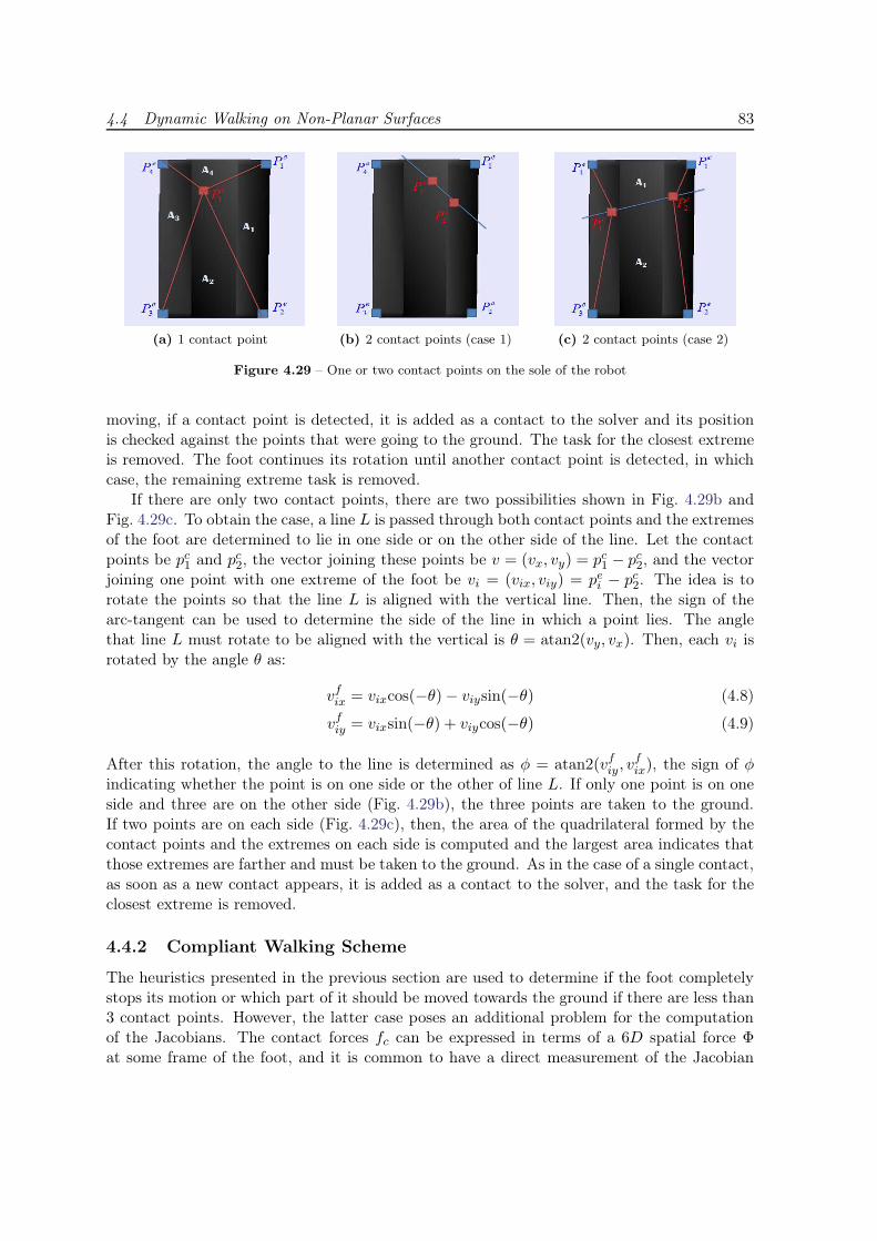
4.4 Dynamic Walking on Non-Planar Surfaces 83
(a) 1 contact point (b) 2 contact points (case 1) (c) 2 contact points (case 2)
Figure 4.29 – One or two contact points on the sole of the robot
moving, if a contact point is detected, it is added as a contact to the solver and its positionis checked against the points that were going to the ground. The task for the closest extremeis removed. The foot continues its rotation until another contact point is detected, in whichcase, the remaining extreme task is removed.
If there are only two contact points, there are two possibilities shown in Fig. 4.29b andFig. 4.29c. To obtain the case, a line L is passed through both contact points and the extremesof the foot are determined to lie in one side or on the other side of the line. Let the contactpoints be pc1 and pc2, the vector joining these points be v = (vx, vy) = pc1 − pc2, and the vectorjoining one point with one extreme of the foot be vi = (vix, viy) = pei − pc2. The idea is torotate the points so that the line L is aligned with the vertical line. Then, the sign of thearc-tangent can be used to determine the side of the line in which a point lies. The anglethat line L must rotate to be aligned with the vertical is θ = atan2(vy, vx). Then, each vi isrotated by the angle θ as:
vfix = vixcos(−θ)− viysin(−θ) (4.8)
vfiy = vixsin(−θ) + viycos(−θ) (4.9)
After this rotation, the angle to the line is determined as φ = atan2(vfiy, vfix), the sign of φ
indicating whether the point is on one side or the other of line L. If only one point is on oneside and three are on the other side (Fig. 4.29b), the three points are taken to the ground.If two points are on each side (Fig. 4.29c), then, the area of the quadrilateral formed by thecontact points and the extremes on each side is computed and the largest area indicates thatthose extremes are farther and must be taken to the ground. As in the case of a single contact,as soon as a new contact appears, it is added as a contact to the solver, and the task for theclosest extreme is removed.
4.4.2 Compliant Walking Scheme
The heuristics presented in the previous section are used to determine if the foot completelystops its motion or which part of it should be moved towards the ground if there are less than3 contact points. However, the latter case poses an additional problem for the computationof the Jacobians. The contact forces fc can be expressed in terms of a 6D spatial force Φat some frame of the foot, and it is common to have a direct measurement of the Jacobian
4.4 Dynamic Walking on Non-Planar Surfaces 84
Figure 4.30 – Compliant walking scheme. The upper level specifies a direction of motion. Then the WPGfinds foot-steps, foot trajectories, a CoM trajectory and a waist trajectory. The Dynamic Stack of Tasks ensuresthat the resulting whole-body motion is dynamically consistent with the robot model and its constraints.
relative to this frame, Jo, which is a geometric Jacobian. Then, the contact Jacobian for thecontact point is computed as in (3.49); that is, Jc = XJo, where X is a matrix involving thecross product with the contact points (3.48). The problem arises from the fact that if thereare only 2 or 1 contact point, X is not full-column rank and the expression for δc in (3.40)has to be modified to δc = −(XJoB)#XJoq. After this modification, the SoT described insection 3.3.4, which explicitly controls the contact force fc, can be directly used.
The compliant walking scheme is obtained by using the output of the WPG as inputto the inverse dynamics solver as shown in Fig. 4.30. The WPG outputs three elements:the trajectory for the CoM, the trajectory for the waist of the robot, and the footprints foreach foot. The usage of these elements within the SoT is done with tracking and interpolationtasks. Tracking tasks are 6D operational tasks described with a PD law and aim to control theposition and/or orientation of a certain characteristic of the robot (the CoM, or an operationalpoint). The interpolation task is a task that takes an operational point from an initial to afinal pose satisfying some fixed (and hard) time constraints, and it has been described in 3.4.3.The dynamic SoT that is used considers the following tasks:
• Tracking task for the horizontal (x, y) components of the CoM trajectory given by theWPG, which assumes a constant height.
• Partial tracking task of the waist trajectory. This task controls the height (position inz) of the waist at a certain constant value, as well as the horizontal orientation in x, y.As observed, not all the six degrees of freedom are controlled, and therefore the nameof partial tracking task.
• Interpolation task on the swinging foot. The WPG gives the footprints on the ground.This task takes the swinging foot from its initial position to its desired final position.There are two interpolation steps: the first task takes the foot from the initial positionon the ground to an intermediate position that lies halfway between the initial and finalpositions with a predetermined height. The second interpolation takes the foot fromthe intermediate to the final position, if possible. The foot reacts in a compliant way ifa contact is detected before arriving to the final position on the ground, as explained insection 4.4.1.
Unlike schemes that only follow the output of the WPG using kinematic tasks, the dynamicSoT makes it possible to handle rough surfaces by adding compliance at the task level to thefoot at the moment of detection of a contact with the environment.
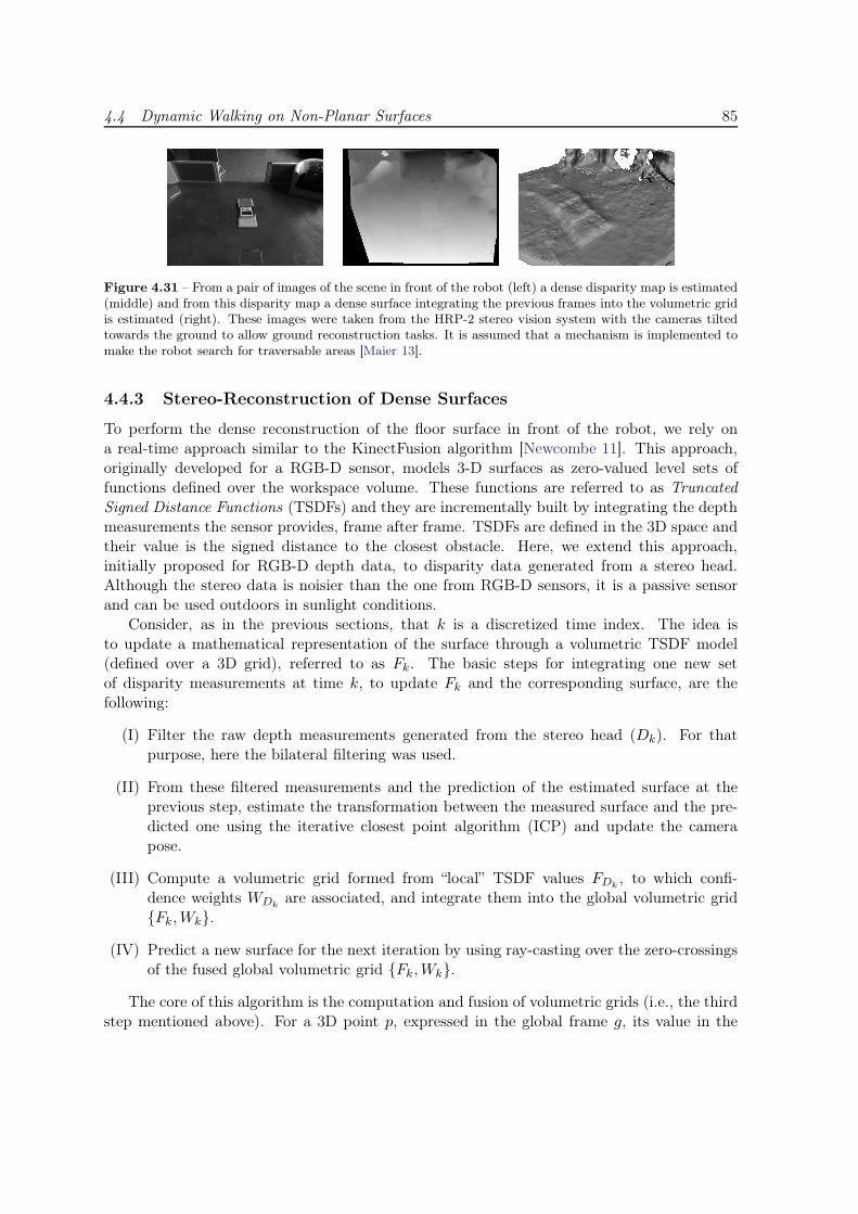
4.4 Dynamic Walking on Non-Planar Surfaces 85
Figure 4.31 – From a pair of images of the scene in front of the robot (left) a dense disparity map is estimated(middle) and from this disparity map a dense surface integrating the previous frames into the volumetric gridis estimated (right). These images were taken from the HRP-2 stereo vision system with the cameras tiltedtowards the ground to allow ground reconstruction tasks. It is assumed that a mechanism is implemented tomake the robot search for traversable areas [Maier 13].
4.4.3 Stereo-Reconstruction of Dense Surfaces
To perform the dense reconstruction of the floor surface in front of the robot, we rely ona real-time approach similar to the KinectFusion algorithm [Newcombe 11]. This approach,originally developed for a RGB-D sensor, models 3-D surfaces as zero-valued level sets offunctions defined over the workspace volume. These functions are referred to as TruncatedSigned Distance Functions (TSDFs) and they are incrementally built by integrating the depthmeasurements the sensor provides, frame after frame. TSDFs are defined in the 3D space andtheir value is the signed distance to the closest obstacle. Here, we extend this approach,initially proposed for RGB-D depth data, to disparity data generated from a stereo head.Although the stereo data is noisier than the one from RGB-D sensors, it is a passive sensorand can be used outdoors in sunlight conditions.
Consider, as in the previous sections, that k is a discretized time index. The idea isto update a mathematical representation of the surface through a volumetric TSDF model(defined over a 3D grid), referred to as Fk. The basic steps for integrating one new setof disparity measurements at time k, to update Fk and the corresponding surface, are thefollowing:
(I) Filter the raw depth measurements generated from the stereo head (Dk). For thatpurpose, here the bilateral filtering was used.
(II) From these filtered measurements and the prediction of the estimated surface at theprevious step, estimate the transformation between the measured surface and the pre-dicted one using the iterative closest point algorithm (ICP) and update the camerapose.
(III) Compute a volumetric grid formed from “local” TSDF values FDk, to which confi-
dence weights WDkare associated, and integrate them into the global volumetric grid
{Fk,Wk}.
(IV) Predict a new surface for the next iteration by using ray-casting over the zero-crossingsof the fused global volumetric grid {Fk,Wk}.
The core of this algorithm is the computation and fusion of volumetric grids (i.e., the thirdstep mentioned above). For a 3D point p, expressed in the global frame g, its value in the
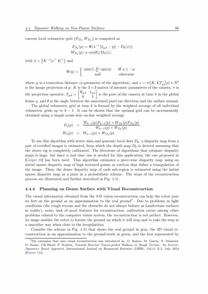
4.4 Dynamic Walking on Non-Planar Surfaces 86
current local volumetric grid {FDk,WDk
} is computed as
FDk(p) = Ψ(λ−1 ‖tg,k − p‖ −Dk(x)),
WDk(p) ∝ cos(θ)/Dk(x),
with λ =∥
∥K−1[x⊤ 1]⊤∥
∥ and
Ψ(η) =
{
min(1, ηµ) sgn(η) iff η ≥ −µ
null otherwise
where µ is a truncation distance (a parameter of the algorithm), and x = π([K,1]T−1g,k p) ∈ R
2
is the image projection of p. K is the 3× 3 matrix of intrinsic parameters of the camera, π is
the projection operator, Tg,k =
[
Rg,k tg,k0 1
]
is the pose of the camera at time k in the global
frame g, and θ is the angle between the associated pixel ray direction and the surface normal.The global volumetric grid at time k is formed by the weighted average of all individual
volumetric grids up to k − 1. It can be shown that the optimal grid can be incrementallyobtained using a simple point-wise on-line weighted average
Fk(p) =Wk−1(p)Fk−1(p) +WDk
(p)FDk(p)
Wk−1(p) +WDk(p)
,
Wk(p) = Wk−1(p) +WDk(p).
To use this algorithm with stereo data and generate local data Dk, a disparity map from apair of rectified images is estimated, from which the depth map Dk is derived assuming thatthe stereo rig is completely calibrated. The literature of algorithms that estimate disparitymaps is huge, but since a real time one is needed for this application, the one proposed in[Geiger 10] has been used. This algorithm estimates a piece-wise disparity map using aninitial sparse disparity map of high textured points as vertices that define a triangulation ofthe image. Then, the dense disparity map of each sub-region is estimated using the initialsparse disparity map as a prior in a probabilistic scheme. The steps of the reconstructionprocess are illustrated and further described in Fig. 4.31.
4.4.4 Planning on Dense Surface with Visual Reconstruction
The visual information obtained from the 3-D vision reconstruction can help the robot poseits feet on the ground as an approximation to the real ground7. Due to problems in lightconditions (the rough terrain and the obstacles do not always behave as Lambertian surfacesin reality), noise, lack of good features for reconstruction, calibration errors among otherproblems related to the computer vision system, the reconstruction is not perfect. However,its usage enables the robot to foresee the ground on which it will step and to take the step ina smoother way when close to the irregularities.
Consider the scheme in Fig. 4.32 that shows the real ground in gray, the 3D visual re-construction as an approximation to the ground-truth in green, and the foot represented by
7The extension that uses visual reconstruction was introduced in: O. Ramos, M. Garcia, N. Mansard,O. Stasse, J-B Hayet, P. Souères, Towards Reactive Vision-guided Walking on Rough Terrain: An Inverse-Dynamics Based Approach, International Journal on Humanoid Robotics (IJHR), Vol.11 N.2, July 2014[Ramos 14a].
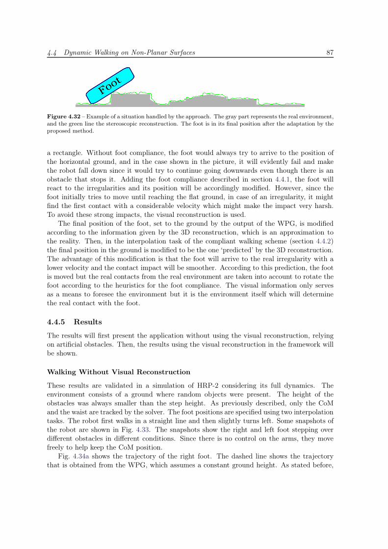
4.4 Dynamic Walking on Non-Planar Surfaces 87
Figure 4.32 – Example of a situation handled by the approach. The gray part represents the real environment,and the green line the stereoscopic reconstruction. The foot is in its final position after the adaptation by theproposed method.
a rectangle. Without foot compliance, the foot would always try to arrive to the position ofthe horizontal ground, and in the case shown in the picture, it will evidently fail and makethe robot fall down since it would try to continue going downwards even though there is anobstacle that stops it. Adding the foot compliance described in section 4.4.1, the foot willreact to the irregularities and its position will be accordingly modified. However, since thefoot initially tries to move until reaching the flat ground, in case of an irregularity, it mightfind the first contact with a considerable velocity which might make the impact very harsh.To avoid these strong impacts, the visual reconstruction is used.
The final position of the foot, set to the ground by the output of the WPG, is modifiedaccording to the information given by the 3D reconstruction, which is an approximation tothe reality. Then, in the interpolation task of the compliant walking scheme (section 4.4.2)the final position in the ground is modified to be the one ‘predicted’ by the 3D reconstruction.The advantage of this modification is that the foot will arrive to the real irregularity with alower velocity and the contact impact will be smoother. According to this prediction, the footis moved but the real contacts from the real environment are taken into account to rotate thefoot according to the heuristics for the foot compliance. The visual information only servesas a means to foresee the environment but it is the environment itself which will determinethe real contact with the foot.
4.4.5 Results
The results will first present the application without using the visual reconstruction, relyingon artificial obstacles. Then, the results using the visual reconstruction in the framework willbe shown.
Walking Without Visual Reconstruction
These results are validated in a simulation of HRP-2 considering its full dynamics. Theenvironment consists of a ground where random objects were present. The height of theobstacles was always smaller than the step height. As previously described, only the CoMand the waist are tracked by the solver. The foot positions are specified using two interpolationtasks. The robot first walks in a straight line and then slightly turns left. Some snapshots ofthe robot are shown in Fig. 4.33. The snapshots show the right and left foot stepping overdifferent obstacles in different conditions. Since there is no control on the arms, they movefreely to help keep the CoM position.
Fig. 4.34a shows the trajectory of the right foot. The dashed line shows the trajectorythat is obtained from the WPG, which assumes a constant ground height. As stated before,
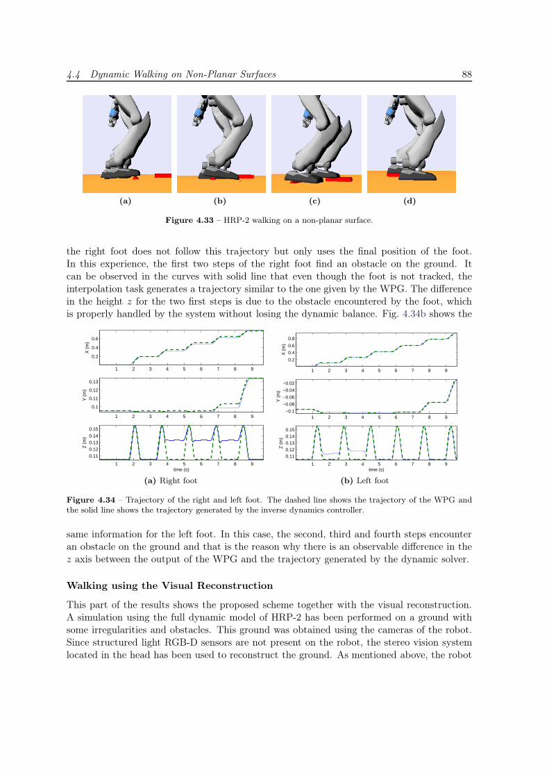
4.4 Dynamic Walking on Non-Planar Surfaces 88
(a) (b) (c) (d)
Figure 4.33 – HRP-2 walking on a non-planar surface.
the right foot does not follow this trajectory but only uses the final position of the foot.In this experience, the first two steps of the right foot find an obstacle on the ground. Itcan be observed in the curves with solid line that even though the foot is not tracked, theinterpolation task generates a trajectory similar to the one given by the WPG. The differencein the height z for the two first steps is due to the obstacle encountered by the foot, whichis properly handled by the system without losing the dynamic balance. Fig. 4.34b shows the
1 2 3 4 5 6 7 8 9
0.2
0.4
0.6
X (
m)
1 2 3 4 5 6 7 8 9
0.1
0.11
0.12
0.13
Y (
m)
1 2 3 4 5 6 7 8 9
0.110.120.130.140.15
Z (
m)
time (s)
(a) Right foot
1 2 3 4 5 6 7 8 9
0.2
0.4
0.6
0.8
X (
m)
1 2 3 4 5 6 7 8 9−0.1
−0.08
−0.06
−0.04
−0.02
Y (
m)
1 2 3 4 5 6 7 8 9
0.110.120.130.140.15
Z (
m)
time (s)
(b) Left foot
Figure 4.34 – Trajectory of the right and left foot. The dashed line shows the trajectory of the WPG andthe solid line shows the trajectory generated by the inverse dynamics controller.
same information for the left foot. In this case, the second, third and fourth steps encounteran obstacle on the ground and that is the reason why there is an observable difference in thez axis between the output of the WPG and the trajectory generated by the dynamic solver.
Walking using the Visual Reconstruction
This part of the results shows the proposed scheme together with the visual reconstruction.A simulation using the full dynamic model of HRP-2 has been performed on a ground withsome irregularities and obstacles. This ground was obtained using the cameras of the robot.Since structured light RGB-D sensors are not present on the robot, the stereo vision systemlocated in the head has been used to reconstruct the ground. As mentioned above, the robot
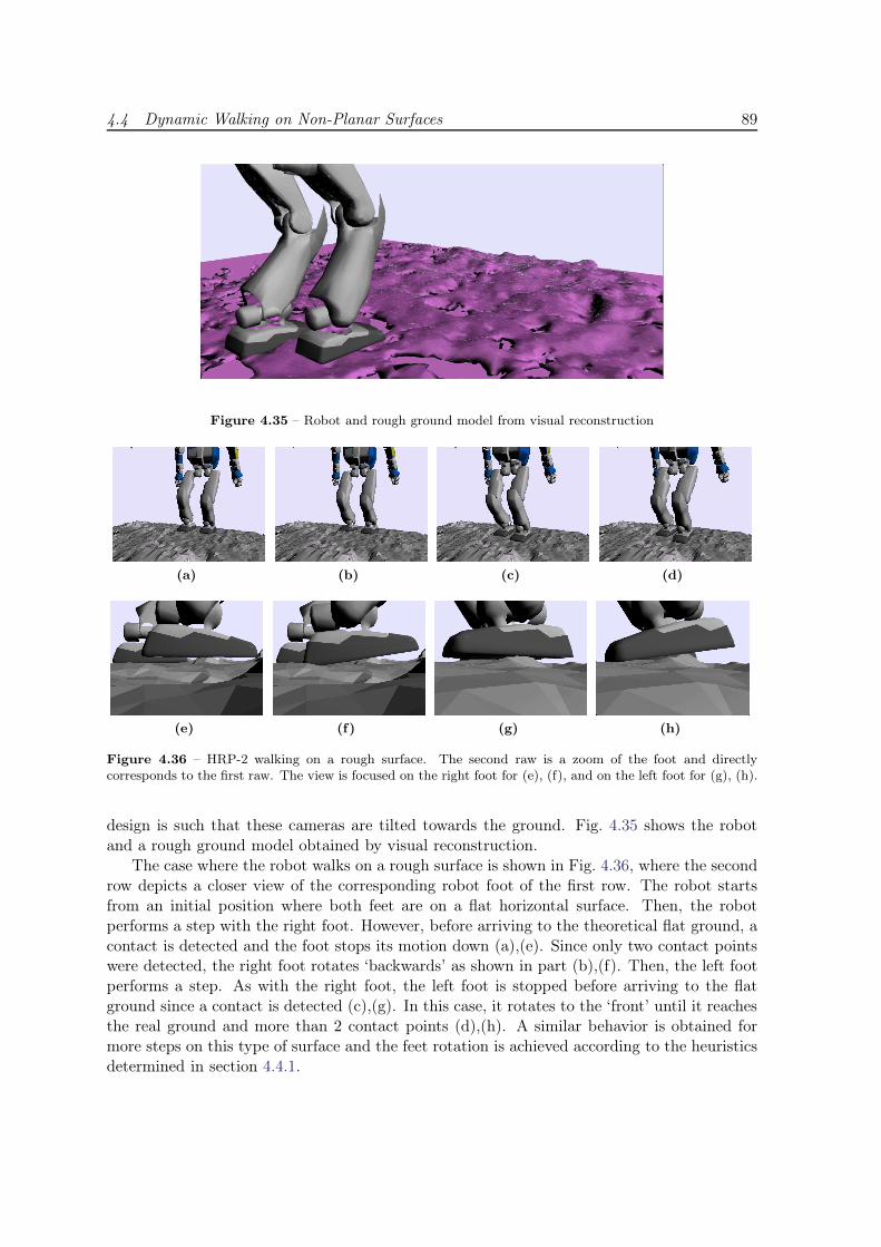
4.4 Dynamic Walking on Non-Planar Surfaces 89
Figure 4.35 – Robot and rough ground model from visual reconstruction
(a) (b) (c) (d)
(e) (f) (g) (h)
Figure 4.36 – HRP-2 walking on a rough surface. The second raw is a zoom of the foot and directlycorresponds to the first raw. The view is focused on the right foot for (e), (f), and on the left foot for (g), (h).
design is such that these cameras are tilted towards the ground. Fig. 4.35 shows the robotand a rough ground model obtained by visual reconstruction.
The case where the robot walks on a rough surface is shown in Fig. 4.36, where the secondrow depicts a closer view of the corresponding robot foot of the first row. The robot startsfrom an initial position where both feet are on a flat horizontal surface. Then, the robotperforms a step with the right foot. However, before arriving to the theoretical flat ground, acontact is detected and the foot stops its motion down (a),(e). Since only two contact pointswere detected, the right foot rotates ‘backwards’ as shown in part (b),(f). Then, the left footperforms a step. As with the right foot, the left foot is stopped before arriving to the flatground since a contact is detected (c),(g). In this case, it rotates to the ‘front’ until it reachesthe real ground and more than 2 contact points (d),(h). A similar behavior is obtained formore steps on this type of surface and the feet rotation is achieved according to the heuristicsdetermined in section 4.4.1.
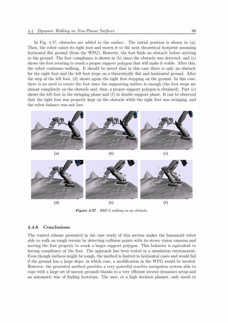
4.4 Dynamic Walking on Non-Planar Surfaces 90
In Fig. 4.37, obstacles are added to the surface. The initial position is shown in (a).Then, the robot raises its right foot and moves it to the next theoretical footprint assuminghorizontal flat ground (from the WPG). However, the foot finds an obstacle before arrivingto the ground. The foot compliance is shown in (b) since the obstacle was detected, and (c)shows the foot rotating to reach a proper support polygon that will make it stable. After this,the robot continues walking. It should be noted that in this case there is only an obstaclefor the right foot and the left foot steps on a theoretically flat and horizontal ground. Afterthe step of the left foot, (d) shows again the right foot stepping on the ground. In this case,there is no need to rotate the foot since the supporting surface is enough (the foot steps arealmost completely on the obstacle and, thus, a proper support polygon is obtained). Part (e)shows the left foot in the swinging phase and (f) in double support phase. It can be observedthat the right foot was properly kept on the obstacle while the right foot was swinging, andthe robot balance was not lost.
(a) (b) (c)
(d) (e) (f)
Figure 4.37 – HRP-2 walking on an obstacle.
4.4.6 Conclusions
The control scheme presented in the case study of this section makes the humanoid robotable to walk on rough terrain by detecting collision points with its stereo vision cameras andmoving the foot properly to reach a larger support polygon. This behavior is equivalent tohaving compliance at the foot. The approach has been tested in a simulation environment.Even though surfaces might be rough, the method is limited to horizontal cases and would failif the ground has a large slope, in which case, a modification in the WPG would be needed.However, the presented method provides a very powerful reactive navigation system able tocope with a large set of uneven grounds thanks to a very efficient inverse dynamics setup andan automatic way of finding footsteps. The user, or a high decision planner, only needs to
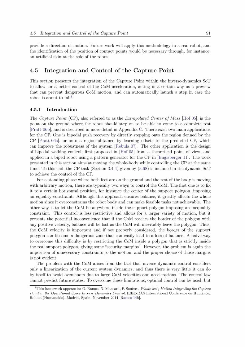
4.5 Integration and Control of the Capture Point 91
provide a direction of motion. Future work will apply this methodology in a real robot, andthe identification of the position of contact points would be necessary through, for instance,an artificial skin at the sole of the robot.
4.5 Integration and Control of the Capture Point
This section presents the integration of the Capture Point within the inverse-dynamics SoTto allow for a better control of the CoM acceleration, acting in a certain way as a previewthat can prevent dangerous CoM motion, and can automatically launch a step in case therobot is about to fall8.
4.5.1 Introduction
The Capture Point (CP), also referred to as the Extrapolated Center of Mass [Hof 05], is thepoint on the ground where the robot should step on to be able to come to a complete rest[Pratt 06b], and is described in more detail in Appendix C. There exist two main applicationsfor the CP. One is bipedal push recovery by directly stepping onto the region defined by theCP [Pratt 06a], or onto a region obtained by learning offsets to the predicted CP, whichcan improve the robustness of the system [Rebula 07]. The other application is the designof bipedal walking control, first proposed in [Hof 05] from a theoretical point of view, andapplied in a biped robot using a pattern generator for the CP in [Englsberger 11]. The workpresented in this section aims at moving the whole-body while controlling the CP at the sametime. To this end, the CP task (Section 3.4.4) given by (3.68) is included in the dynamic SoTto achieve the control of the CP.
For a standing phase where both feet are on the ground and the rest of the body is movingwith arbitrary motion, there are typically two ways to control the CoM. The first one is to fixit to a certain horizontal position, for instance the center of the support polygon, imposingan equality constraint. Although this approach ensures balance, it greatly affects the wholemotion since it overconstrains the robot body and can make feasible tasks not achievable. Theother way is to let the CoM lie anywhere inside the support polygon imposing an inequalityconstraint. This control is less restrictive and allows for a larger variety of motion, but itpresents the potential inconvenience that if the CoM reaches the border of the polygon withany positive velocity, balance will be lost as the CoM will inevitably leave the polygon. Thus,the CoM velocity is important and if not properly considered, the border of the supportpolygon can become a dangerous zone that can easily lead to a loss of balance. A naive wayto overcome this difficulty is by restricting the CoM inside a polygon that is strictly insidethe real support polygon, giving some “security margins”. However, the problem is again theimposition of unnecessary constraints to the motion, and the proper choice of those marginsis not evident.
The problem with the CoM arises from the fact that inverse dynamics control considersonly a linearization of the current system dynamics, and thus there is very little it can doby itself to avoid overshoots due to large CoM velocities and accelerations. The control lawcannot predict future states. To overcome these limitations, optimal control can be used, but
8This framework appears in: O. Ramos, N. Mansard, P. Souères, Whole-body Motion Integrating the CapturePoint in the Operational Space Inverse Dynamics Control, IEEE-RAS International Conference on HumanoidRobots (Humanoids), Madrid, Spain, November 2014 [Ramos 14b].
4.5 Integration and Control of the Capture Point 92
it is currently computationally very expensive. The approach in this section rather proposesto preview the CoM future through the CP, and therefore to constrain the CoM velocity at thelimit using the CP as a measurement of its future, since both quantities are related, as (3.66)shows. While the CP remains inside the support polygon, the robot is able to freely move itswhole-body with the consideration that there will always exist the possibility to come to rest.That is, the robot keeps and will keep its balance. If the CP leaves the support polygon whileperforming some fast motion, it will not be possible for the robot to come to rest in doublesupport and, unless a step is taken, balance will be lost. Then, a task to impose a constrainton the CP can be a good solution.
The approach presented in this section aims at directly bounding the CoM velocity bycontrolling the CP, since both quantities are related, as (3.66) shows. If the CP remains insidethe support polygon, the robot will be able to freely move with the consideration that therewill always exist the possibility to come to rest. That is, the robot will be stable. If the CPis out of the support polygon, it will not be possible for the robot to come to rest in doublesupport and, unless a step is taken, it will lose its balance. Thus, the CP task is proposedinside the OSID control as an inequality task to keep the CP inside the support polygon.Moreover, this task can further be used with a “larger” support polygon, in which case, a stepwill be required, but the CP will not move without bounds, making the step feasible. Thefact of controlling the CP as a task implies that it will not escape the pre-defined polygon byimplicitly constraining the whole motion of the robot. The implicit constraints might appearas motion of the parts of the robot for which no task is specified (for instance, an arm or thechest) in an attempt to compensate the otherwise fast falling motion.
4.5.2 Scheme for the Capture Point Control
The first use of the CP task introduced in Section 3.4.4 is to directly keep the CP inside thereal support polygon. This is done by defining the limits of the task (rp and rp) in termsof the real support polygon as in (3.68). The CP task is then added to the dynamic SoT,described in section 3.3.3, as an inequality task with a priority higher than the rest of thetasks, so that it is satisfied in all the cases. This leads to a more restrictive control thansimply constraining the CoM within the support polygon, but it has the advantage that theCoM velocity is also controlled. This implies that the CoM at the borders of the polygon willnot present high velocities that make it irreversibly exit the polygon. The reason is that bydefinition, if the CP is always kept inside the polygon, the CoM will be able to come to a restwithin it in finite time. In other terms, the robot will be able to move without falling.
However, there are situations where the fulfillment of a task might require to move theCoM away from the support polygon (for example, if the robot has to reach an object thatis farther than roughly the length of its arm), which would cause a loss of balance. For thesecases, the strict balance condition can be relaxed by defining a polygon outside the limitsof the real support polygon, but within an area that is reachable by a step, as Fig. 4.38shows. Then, this ‘extended’ polygon is used as limit for the position of the CP. Providedthat double support balance is lost, a step towards the CP will have to be taken to recoverbalance; otherwise the robot will fall. This scheme is summarized as follows:
• Definition of the Capture Point task. An ‘extended’ polygon covering the area that isreachable by the robot foot is defined as limit for the CP task. This will constrain
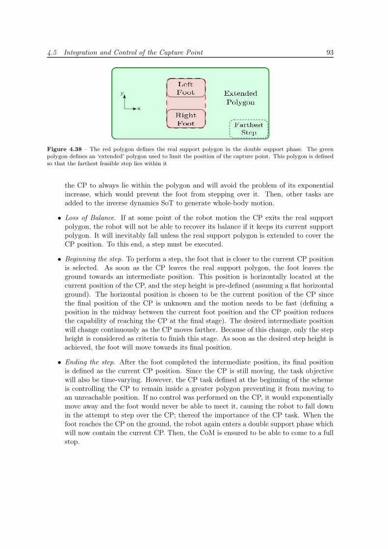
4.5 Integration and Control of the Capture Point 93
Figure 4.38 – The red polygon defines the real support polygon in the double support phase. The greenpolygon defines an ‘extended’ polygon used to limit the position of the capture point. This polygon is definedso that the farthest feasible step lies within it
the CP to always lie within the polygon and will avoid the problem of its exponentialincrease, which would prevent the foot from stepping over it. Then, other tasks areadded to the inverse dynamics SoT to generate whole-body motion.
• Loss of Balance. If at some point of the robot motion the CP exits the real supportpolygon, the robot will not be able to recover its balance if it keeps its current supportpolygon. It will inevitably fall unless the real support polygon is extended to cover theCP position. To this end, a step must be executed.
• Beginning the step. To perform a step, the foot that is closer to the current CP positionis selected. As soon as the CP leaves the real support polygon, the foot leaves theground towards an intermediate position. This position is horizontally located at thecurrent position of the CP, and the step height is pre-defined (assuming a flat horizontalground). The horizontal position is chosen to be the current position of the CP sincethe final position of the CP is unknown and the motion needs to be fast (defining aposition in the midway between the current foot position and the CP position reducesthe capability of reaching the CP at the final stage). The desired intermediate positionwill change continuously as the CP moves farther. Because of this change, only the stepheight is considered as criteria to finish this stage. As soon as the desired step height isachieved, the foot will move towards its final position.
• Ending the step. After the foot completed the intermediate position, its final positionis defined as the current CP position. Since the CP is still moving, the task objectivewill also be time-varying. However, the CP task defined at the beginning of the schemeis controlling the CP to remain inside a greater polygon preventing it from moving toan unreachable position. If no control was performed on the CP, it would exponentiallymove away and the foot would never be able to meet it, causing the robot to fall downin the attempt to step over the CP; thereof the importance of the CP task. When thefoot reaches the CP on the ground, the robot again enters a double support phase whichwill now contain the current CP. Then, the CoM is ensured to be able to come to a fullstop.
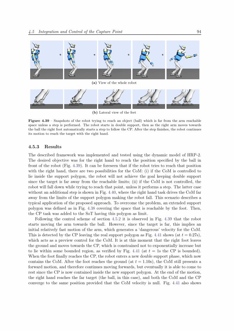
4.5 Integration and Control of the Capture Point 94
(a) View of the whole robot
(b) Lateral view of the feet
Figure 4.39 – Snapshots of the robot trying to reach an object (ball) which is far from the arm reachablespace unless a step is performed. The robot starts in double support, then as the right arm moves towardsthe ball the right foot automatically starts a step to follow the CP. After the step finishes, the robot continuesits motion to reach the target with the right hand.
4.5.3 Results
The described framework was implemented and tested using the dynamic model of HRP-2.The desired objective was for the right hand to reach the position specified by the ball infront of the robot (Fig. 4.39). It can be foreseen that if the robot tries to reach that positionwith the right hand, there are two possibilities for the CoM: (i) if the CoM is controlled tolie inside the support polygon, the robot will not achieve the goal keeping double supportsince the target is far away from the reachable limits; (ii) if the CoM is not controlled, therobot will fall down while trying to reach that point, unless it performs a step. The latter casewithout an additional step is shown in Fig. 4.40, where the right hand task drives the CoM faraway from the limits of the support polygon making the robot fall. This scenario describes atypical application of the proposed approach. To overcome the problem, an extended supportpolygon was defined as in Fig. 4.38 covering the space that is reachable by the foot. Then,the CP task was added to the SoT having this polygon as limit.
Following the control scheme of section 4.5.2 it is observed in Fig. 4.39 that the robotstarts moving the arm towards the ball. However, since the target is far, this implies aninitial relatively fast motion of the arm, which generates a ‘dangerous’ velocity for the CoM.This is detected by the CP leaving the real support polygon as Fig. 4.41 shows (at t = 0.27s),which acts as a preview control for the CoM. It is at this moment that the right foot leavesthe ground and moves towards the CP, which is constrained not to exponentially increase butto lie within some bounded region, as verified by Fig. 4.41 (at t = 1s the CP is bounded).When the foot finally reaches the CP, the robot enters a new double support phase, which nowcontains the CoM. After the foot reaches the ground (at t = 1.10s), the CoM still presents aforward motion, and therefore continues moving forwards, but eventually it is able to come torest since the CP is now contained inside the new support polygon. At the end of the motion,the right hand reaches the far target (the ball, in this case), and both the CoM and the CPconverge to the same position provided that the CoM velocity is null. Fig. 4.41 also shows
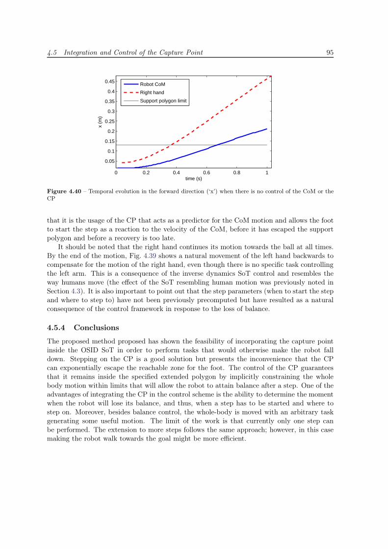
4.5 Integration and Control of the Capture Point 95
0 0.2 0.4 0.6 0.8 1
0.05
0.1
0.15
0.2
0.25
0.3
0.35
0.4
0.45
time (s)
x (m
)
Robot CoM
Right hand
Support polygon limit
Figure 4.40 – Temporal evolution in the forward direction (‘x’) when there is no control of the CoM or theCP
that it is the usage of the CP that acts as a predictor for the CoM motion and allows the footto start the step as a reaction to the velocity of the CoM, before it has escaped the supportpolygon and before a recovery is too late.
It should be noted that the right hand continues its motion towards the ball at all times.By the end of the motion, Fig. 4.39 shows a natural movement of the left hand backwards tocompensate for the motion of the right hand, even though there is no specific task controllingthe left arm. This is a consequence of the inverse dynamics SoT control and resembles theway humans move (the effect of the SoT resembling human motion was previously noted inSection 4.3). It is also important to point out that the step parameters (when to start the stepand where to step to) have not been previously precomputed but have resulted as a naturalconsequence of the control framework in response to the loss of balance.
4.5.4 Conclusions
The proposed method proposed has shown the feasibility of incorporating the capture pointinside the OSID SoT in order to perform tasks that would otherwise make the robot falldown. Stepping on the CP is a good solution but presents the inconvenience that the CPcan exponentially escape the reachable zone for the foot. The control of the CP guaranteesthat it remains inside the specified extended polygon by implicitly constraining the wholebody motion within limits that will allow the robot to attain balance after a step. One of theadvantages of integrating the CP in the control scheme is the ability to determine the momentwhen the robot will lose its balance, and thus, when a step has to be started and where tostep on. Moreover, besides balance control, the whole-body is moved with an arbitrary taskgenerating some useful motion. The limit of the work is that currently only one step canbe performed. The extension to more steps follows the same approach; however, in this casemaking the robot walk towards the goal might be more efficient.
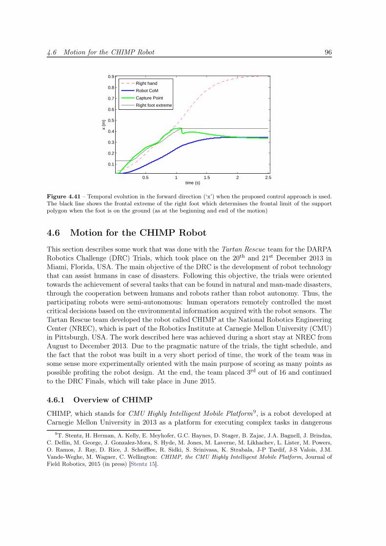
4.6 Motion for the CHIMP Robot 96
0.5 1 1.5 2 2.5
0.1
0.2
0.3
0.4
0.5
0.6
0.7
0.8
0.9
time (s)
x (m
)
Right hand
Robot CoM
Capture Point
Right foot extreme
Figure 4.41 – Temporal evolution in the forward direction (‘x’) when the proposed control approach is used.The black line shows the frontal extreme of the right foot which determines the frontal limit of the supportpolygon when the foot is on the ground (as at the beginning and end of the motion)
4.6 Motion for the CHIMP Robot
This section describes some work that was done with the Tartan Rescue team for the DARPARobotics Challenge (DRC) Trials, which took place on the 20th and 21st December 2013 inMiami, Florida, USA. The main objective of the DRC is the development of robot technologythat can assist humans in case of disasters. Following this objective, the trials were orientedtowards the achievement of several tasks that can be found in natural and man-made disasters,through the cooperation between humans and robots rather than robot autonomy. Thus, theparticipating robots were semi-autonomous: human operators remotely controlled the mostcritical decisions based on the environmental information acquired with the robot sensors. TheTartan Rescue team developed the robot called CHIMP at the National Robotics EngineeringCenter (NREC), which is part of the Robotics Institute at Carnegie Mellon University (CMU)in Pittsburgh, USA. The work described here was achieved during a short stay at NREC fromAugust to December 2013. Due to the pragmatic nature of the trials, the tight schedule, andthe fact that the robot was built in a very short period of time, the work of the team was insome sense more experimentally oriented with the main purpose of scoring as many points aspossible profiting the robot design. At the end, the team placed 3rd out of 16 and continuedto the DRC Finals, which will take place in June 2015.
4.6.1 Overview of CHIMP
CHIMP, which stands for CMU Highly Intelligent Mobile Platform9, is a robot developed atCarnegie Mellon University in 2013 as a platform for executing complex tasks in dangerous
9T. Stentz, H. Herman, A. Kelly, E. Meyhofer, G.C. Haynes, D. Stager, B. Zajac, J.A. Bagnell, J. Brindza,C. Dellin, M. George, J. Gonzalez-Mora, S. Hyde, M. Jones, M. Laverne, M. Likhachev, L. Lister, M. Powers,O. Ramos, J. Ray, D. Rice, J. Scheifflee, R. Sidki, S. Srinivasa, K. Strabala, J-P Tardif, J-S Valois, J.M.Vande-Weghe, M. Wagner, C. Wellington: CHIMP, the CMU Highly Intelligent Mobile Platform, Journal ofField Robotics, 2015 (in press) [Stentz 15].
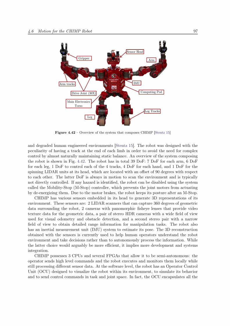
4.6 Motion for the CHIMP Robot 97
Gripper
Arm tracks
Drive Joint (30X)
Main ElectronicsTorso
Leg
Sensor Head
Arm
Computing Pod
Leg Tracks
IMU
Figure 4.42 – Overview of the system that composes CHIMP [Stentz 15]
and degraded human engineered environments [Stentz 15]. The robot was designed with thepeculiarity of having a track at the end of each limb in order to avoid the need for complexcontrol by almost naturally maintaining static balance. An overview of the system composingthe robot is shown in Fig. 4.42. The robot has in total 39 DoF: 7 DoF for each arm, 6 DoFfor each leg, 1 DoF to control each of the 4 tracks, 4 DoF for each hand, and 1 DoF for thespinning LIDAR units at its head, which are located with an offset of 90 degrees with respectto each other. The latter DoF is always in motion to scan the environment and is typicallynot directly controlled. If any hazard is identified, the robot can be disabled using the systemcalled the Mobility-Stop (M-Stop) controller, which prevents the joint motors from actuatingby de-energizing them. Due to the motor brakes, the robot keeps its posture after an M-Stop.
CHIMP has various sensors embedded in its head to generate 3D representations of itsenvironment. These sensors are: 2 LIDAR scanners that can capture 360 degrees of geometricdata surrounding the robot, 2 cameras with panomorphic fisheye lenses that provide videotexture data for the geometric data, a pair of stereo HDR cameras with a wide field of viewused for visual odometry and obstacle detection, and a second stereo pair with a narrowfield of view to obtain detailed range information for manipulation tasks. The robot alsohas an inertial measurement unit (IMU) system to estimate its pose. The 3D reconstructionobtained with the sensors is currently used to help human operators understand the robotenvironment and take decisions rather than to autonomously process the information. Whilethe latter choice would arguably be more efficient, it implies more development and systemsintegration.
CHIMP possesses 3 CPUs and several FPGAs that allow it to be semi-autonomous: theoperator sends high level commands and the robot executes and monitors them locally whilestill processing different sensor data. At the software level, the robot has an Operator ControlUnit (OCU) designed to visualize the robot within its environment, to simulate its behaviorand to send control commands in task and joint space. In fact, the OCU encapsulates all the
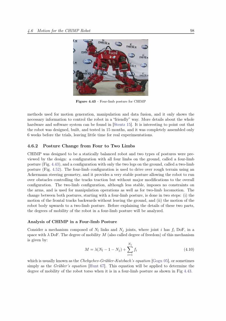
4.6 Motion for the CHIMP Robot 98
Figure 4.43 – Four-limb posture for CHIMP
methods used for motion generation, manipulation and data fusion, and it only shows thenecessary information to control the robot in a “friendly” way. More details about the wholehardware and software system can be found in [Stentz 15]. It is interesting to point out thatthe robot was designed, built, and tested in 15 months, and it was completely assembled only6 weeks before the trials, leaving little time for real experimentations.
4.6.2 Posture Change from Four to Two Limbs
CHIMP was designed to be a statically balanced robot and two types of postures were pre-viewed by the design: a configuration with all four limbs on the ground, called a four-limbposture (Fig. 4.43), and a configuration with only the two legs on the ground, called a two-limbposture (Fig. 4.52). The four-limb configuration is used to drive over rough terrain using anAckermann steering geometry, and it provides a very stable posture allowing the robot to runover obstacles controlling the tracks traction but without major modifications to the overallconfiguration. The two-limb configuration, although less stable, imposes no constraints onthe arms, and is used for manipulation operations as well as for two-limb locomotion. Thechange between both postures, starting with a four-limb posture, is done in two steps: (i) themotion of the frontal tracks backwards without leaving the ground, and (ii) the motion of therobot body upwards to a two-limb posture. Before explaining the details of these two parts,the degrees of mobility of the robot in a four-limb posture will be analyzed.
Analysis of CHIMP in a Four-limb Posture
Consider a mechanism composed of Nl links and Nj joints, where joint i has fi DoF, in aspace with λ DoF. The degree of mobility M (also called degree of freedom) of this mechanismis given by:
M = λ(Nl − 1−Nj) +
Nj∑
i=1
fi (4.10)
which is usually known as the Chebychev-Grübler-Kutzbach’s equation [Gogu 05], or sometimessimply as the Grübler’s equation [Hunt 67]. This equation will be applied to determine thedegree of mobility of the robot torso when it is in a four-limb posture as shown in Fig 4.43.
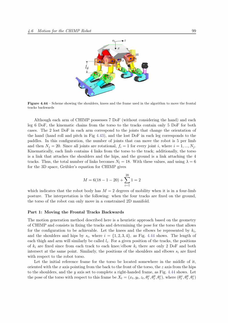
4.6 Motion for the CHIMP Robot 99
k1k2
k3k4
s1s2s3s4l4
z
x
ot
Figure 4.44 – Scheme showing the shoulders, knees and the frame used in the algorithm to move the frontaltracks backwards
Although each arm of CHIMP possesses 7 DoF (without considering the hand) and eachleg 6 DoF, the kinematic chains from the torso to the tracks contain only 5 DoF for bothcases. The 2 lost DoF in each arm correspond to the joints that change the orientation ofthe hand (hand roll and pitch in Fig 4.43), and the lost DoF in each leg corresponds to thepaddles. In this configuration, the number of joints that can move the robot is 5 per limband then Nj = 20. Since all joints are rotational, fi = 1 for every joint i, where i = 1, ..., Nj .Kinematically, each limb contains 4 links from the torso to the track; additionally, the torsois a link that attaches the shoulders and the hips, and the ground is a link attaching the 4tracks. Thus, the total number of links becomes Nl = 18. With these values, and using λ = 6for the 3D space, Grübler’s equation for CHIMP gives
M = 6(18 − 1− 20) +
20∑
i=1
1 = 2
which indicates that the robot body has M = 2 degrees of mobility when it is in a four-limbposture. The interpretation is the following: when the four tracks are fixed on the ground,the torso of the robot can only move in a constrained 2D manifold.
Part 1: Moving the Frontal Tracks Backwards
The motion generation method described here is a heuristic approach based on the geometryof CHIMP and consists in fixing the tracks and determining the pose for the torso that allowsfor the configuration to be achievable. Let the knees and the elbows be represented by ki,and the shoulders and hips by si, where i = {1, 2, 3, 4}, as Fig. 4.44 shows. The length ofeach thigh and arm will similarly be called li. For a given position of the tracks, the positionsof ki are fixed since from each track to each knee/elbow ki there are only 2 DoF and bothintersect at the same point. Similarly, the positions of the shoulders and elbows si are fixedwith respect to the robot torso.
Let the initial reference frame for the torso be located somewhere in the middle of it,oriented with the x axis pointing from the back to the front of the torso, the z axis from the hipsto the shoulders, and the y axis set to complete a right-handed frame, as Fig. 4.44 shows. Letthe pose of the torso with respect to this frame be Xt = (xt, yt, zt, θ
xt , θ
yt , θ
zt ), where (θxt , θ
yt , θ
zt )
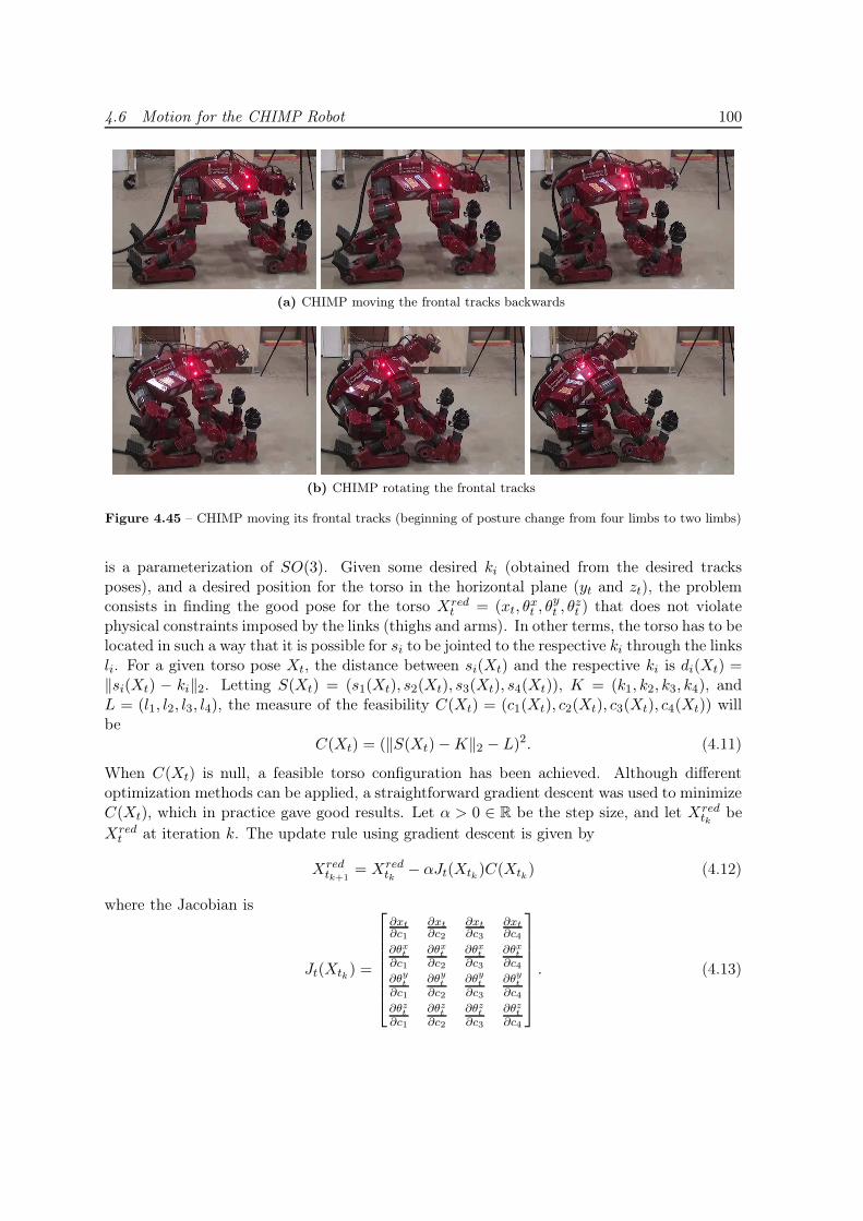
4.6 Motion for the CHIMP Robot 100
(a) CHIMP moving the frontal tracks backwards
(b) CHIMP rotating the frontal tracks
Figure 4.45 – CHIMP moving its frontal tracks (beginning of posture change from four limbs to two limbs)
is a parameterization of SO(3). Given some desired ki (obtained from the desired tracksposes), and a desired position for the torso in the horizontal plane (yt and zt), the problemconsists in finding the good pose for the torso Xred
t = (xt, θxt , θ
yt , θ
zt ) that does not violate
physical constraints imposed by the links (thighs and arms). In other terms, the torso has to belocated in such a way that it is possible for si to be jointed to the respective ki through the linksli. For a given torso pose Xt, the distance between si(Xt) and the respective ki is di(Xt) =‖si(Xt) − ki‖2. Letting S(Xt) = (s1(Xt), s2(Xt), s3(Xt), s4(Xt)), K = (k1, k2, k3, k4), andL = (l1, l2, l3, l4), the measure of the feasibility C(Xt) = (c1(Xt), c2(Xt), c3(Xt), c4(Xt)) willbe
C(Xt) = (‖S(Xt)−K‖2 − L)2. (4.11)
When C(Xt) is null, a feasible torso configuration has been achieved. Although differentoptimization methods can be applied, a straightforward gradient descent was used to minimizeC(Xt), which in practice gave good results. Let α > 0 ∈ R be the step size, and let Xred
tkbe
Xredt at iteration k. The update rule using gradient descent is given by
Xredtk+1
= Xredtk
− αJt(Xtk )C(Xtk) (4.12)
where the Jacobian is
Jt(Xtk ) =
∂xt∂c1
∂xt∂c2
∂xt∂c3
∂xt∂c4
∂θxt∂c1
∂θxt∂c2
∂θxt∂c3
∂θxt∂c4
∂θyt
∂c1
∂θyt
∂c2
∂θyt
∂c3
∂θyt
∂c4
∂θzt∂c1
∂θzt∂c2
∂θzt∂c3
∂θzt∂c4
. (4.13)

4.6 Motion for the CHIMP Robot 101
Figure 4.46 – CHIMP moving to its final 2 limb posture (second part of posture change from four limbs totwo limbs)
After determining a suitable torso pose Xt, inverse kinematics is used to get the jointconfigurations for each limb. Using this method, the results shown in Fig. 4.45 were obtained.In Fig. 4.45a, the pose for the frontal tracks is continuously changed backwards and the poseof the torso is accordingly found. Once the projection of the CoM on the ground lies insidethe polygon formed by the leg tracks, the frontal tracks can leave the ground to a two-limbposture. However, to facilitate the transition and to move the CoM to a safer position, thefrontal tracks are further rotated following the same method, as Fig. 4.45b shows.
Part 2: Moving the Frontal Tracks Upwards
After the CoM projection lies inside the polygon formed by the leg tracks, the frontal trackscan leave the ground without affecting the robot balance. Once the frontal tracks leave theground, the torso gains DoF and its pose is no longer constrained to a 2D manifold. To achievea final pre-defined posture, the motion was decoupled in two parts: the first concerns the legsand the second the arms. The three joints at hips of CHIMP intersect at a single point andpresent a particular configuration similar to a Z-Y-Z mechanism. Consequently, to achievea rotation of the hips about an arbitrary axis, the transformation between the axis-anglerepresentation and the Z-Y-Z Euler angles can be directly used, and the rotation angles in Z,Y and Z correspond directly to each joint at the hip. Profiting this fact, the increment ∆θhabout the world y axis (oriented laterally) was successively given to the hips and the sameincrement but in an opposite direction ∆θk = −∆θh was given to the knee joints. For thearms, a cubic interpolation that accepts intermediate waypoints was used. The results areshown in Fig. 4.46 where the robot starts where Fig. 4.45 stopped and ends up in a two-limbposture which, in this case, is used for two-limb locomotion.
4.6.3 Speed and Acceleration Limits for Locomotion
Since one of the design criteria for the robot was to be statically balanced, special care had tobe taken when making the robot move using the tracks. A very fast initial acceleration or asudden stop when the robot has a high velocity can make it lose balance unless some controlis applied to compensate for the destabilization. However, when the M-stop (Section 4.6.1) isapplied, all the motors are de-energized and there is no possibility to apply a compensating
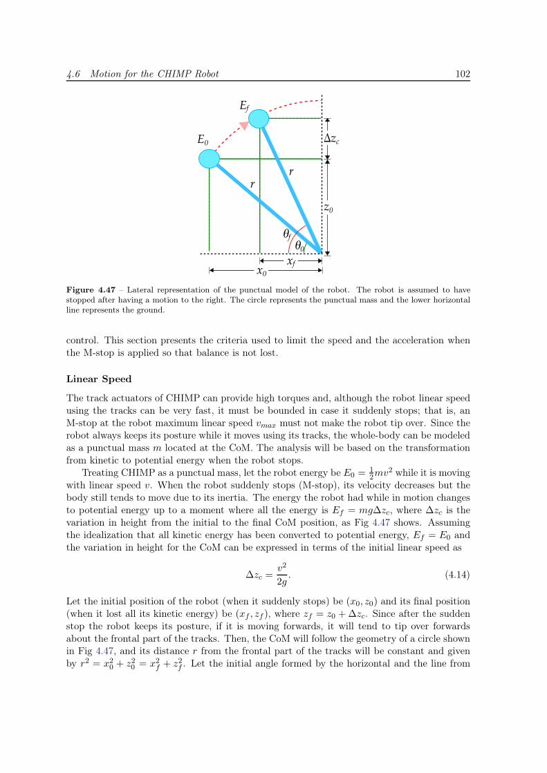
4.6 Motion for the CHIMP Robot 102
Ef
E0
rr
z0
∆zc
xfx0
θ0
θf
Figure 4.47 – Lateral representation of the punctual model of the robot. The robot is assumed to havestopped after having a motion to the right. The circle represents the punctual mass and the lower horizontalline represents the ground.
control. This section presents the criteria used to limit the speed and the acceleration whenthe M-stop is applied so that balance is not lost.
Linear Speed
The track actuators of CHIMP can provide high torques and, although the robot linear speedusing the tracks can be very fast, it must be bounded in case it suddenly stops; that is, anM-stop at the robot maximum linear speed vmax must not make the robot tip over. Since therobot always keeps its posture while it moves using its tracks, the whole-body can be modeledas a punctual mass m located at the CoM. The analysis will be based on the transformationfrom kinetic to potential energy when the robot stops.
Treating CHIMP as a punctual mass, let the robot energy be E0 =12mv
2 while it is movingwith linear speed v. When the robot suddenly stops (M-stop), its velocity decreases but thebody still tends to move due to its inertia. The energy the robot had while in motion changesto potential energy up to a moment where all the energy is Ef = mg∆zc, where ∆zc is thevariation in height from the initial to the final CoM position, as Fig 4.47 shows. Assumingthe idealization that all kinetic energy has been converted to potential energy, Ef = E0 andthe variation in height for the CoM can be expressed in terms of the initial linear speed as
∆zc =v2
2g. (4.14)
Let the initial position of the robot (when it suddenly stops) be (x0, z0) and its final position(when it lost all its kinetic energy) be (xf , zf ), where zf = z0 +∆zc. Since after the suddenstop the robot keeps its posture, if it is moving forwards, it will tend to tip over forwardsabout the frontal part of the tracks. Then, the CoM will follow the geometry of a circle shownin Fig 4.47, and its distance r from the frontal part of the tracks will be constant and givenby r2 = x20 + z20 = x2f + z2f . Let the initial angle formed by the horizontal and the line from
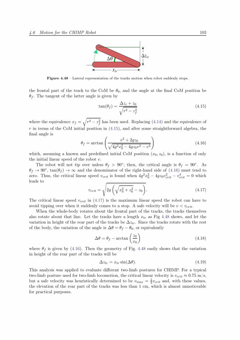
4.6 Motion for the CHIMP Robot 103
xtr
∆θ∆ztr
Figure 4.48 – Lateral representation of the tracks motion when robot suddenly stops.
the frontal part of the track to the CoM be θ0, and the angle at the final CoM position beθf . The tangent of the latter angle is given by
tan(θf ) =∆zc + z0√
r2 − z2f
(4.15)
where the equivalence xf =√
r2 − z2f has been used. Replacing (4.14) and the equivalence of
r in terms of the CoM initial position in (4.15), and after some straightforward algebra, thefinal angle is
θf = arctan
(
v2 + 2gz0√
4g2x20 − 4gz0v2 − v4
)
(4.16)
which, assuming a known and predefined initial CoM position (x0, z0), is a function of onlythe initial linear speed of the robot v.
The robot will not tip over unless θf > 90◦; then, the critical angle is θf = 90◦. Asθf → 90◦, tan(θf ) → ∞ and the denominator of the right-hand side of (4.16) must tend tozero. Thus, the critical linear speed vcrit is found when 4g2x20 − 4gz0v
2crit − v4crit = 0 which
leads to
vcrit =
√
2g
(
√
x20 + z20 − z0
)
. (4.17)
The critical linear speed vcrit in (4.17) is the maximum linear speed the robot can have toavoid tipping over when it suddenly comes to a stop. A safe velocity will be v < vcrit.
When the whole-body rotates about the frontal part of the tracks, the tracks themselvesalso rotate about that line. Let the tracks have a length xtr as Fig 4.48 shows, and let thevariation in height of the rear part of the tracks be ∆ztr. Since the tracks rotate with the restof the body, the variation of the angle is ∆θ = θf − θ0, or equivalently
∆θ = θf − arctan
(
z0x0
)
(4.18)
where θf is given by (4.16). Then the geometry of Fig. 4.48 easily shows that the variationin height of the rear part of the tracks will be
∆ztr = xtr sin(∆θ). (4.19)
This analysis was applied to evaluate different two-limb postures for CHIMP. For a typicaltwo-limb posture used for two-limb locomotion, the critical linear velocity is vcrit ≈ 0.75 m/s,but a safe velocity was heuristically determined to be vmax = 1
3vcrit and, with these values,the elevation of the rear part of the tracks was less than 1 cm, which is almost unnoticeablefor practical purposes.
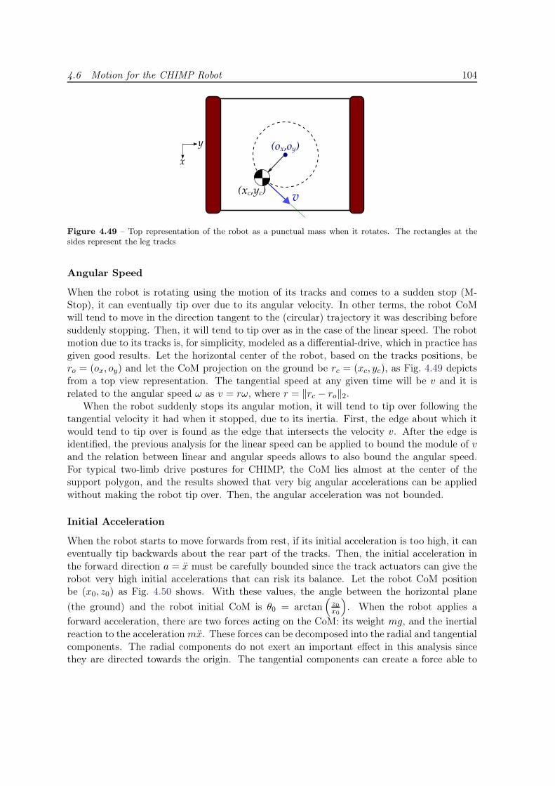
4.6 Motion for the CHIMP Robot 104
(xc,yc)
(ox,oy)
v
x
y
Figure 4.49 – Top representation of the robot as a punctual mass when it rotates. The rectangles at thesides represent the leg tracks
Angular Speed
When the robot is rotating using the motion of its tracks and comes to a sudden stop (M-Stop), it can eventually tip over due to its angular velocity. In other terms, the robot CoMwill tend to move in the direction tangent to the (circular) trajectory it was describing beforesuddenly stopping. Then, it will tend to tip over as in the case of the linear speed. The robotmotion due to its tracks is, for simplicity, modeled as a differential-drive, which in practice hasgiven good results. Let the horizontal center of the robot, based on the tracks positions, bero = (ox, oy) and let the CoM projection on the ground be rc = (xc, yc), as Fig. 4.49 depictsfrom a top view representation. The tangential speed at any given time will be v and it isrelated to the angular speed ω as v = rω, where r = ‖rc − ro‖2.
When the robot suddenly stops its angular motion, it will tend to tip over following thetangential velocity it had when it stopped, due to its inertia. First, the edge about which itwould tend to tip over is found as the edge that intersects the velocity v. After the edge isidentified, the previous analysis for the linear speed can be applied to bound the module of vand the relation between linear and angular speeds allows to also bound the angular speed.For typical two-limb drive postures for CHIMP, the CoM lies almost at the center of thesupport polygon, and the results showed that very big angular accelerations can be appliedwithout making the robot tip over. Then, the angular acceleration was not bounded.
Initial Acceleration
When the robot starts to move forwards from rest, if its initial acceleration is too high, it caneventually tip backwards about the rear part of the tracks. Then, the initial acceleration inthe forward direction a = x must be carefully bounded since the track actuators can give therobot very high initial accelerations that can risk its balance. Let the robot CoM positionbe (x0, z0) as Fig. 4.50 shows. With these values, the angle between the horizontal plane
(the ground) and the robot initial CoM is θ0 = arctan(
z0x0
)
. When the robot applies a
forward acceleration, there are two forces acting on the CoM: its weight mg, and the inertialreaction to the acceleration mx. These forces can be decomposed into the radial and tangentialcomponents. The radial components do not exert an important effect in this analysis sincethey are directed towards the origin. The tangential components can create a force able to

4.6 Motion for the CHIMP Robot 105
mg
ma
masin(θ)
mgcos(θ)
θ0
x0
z0
Figure 4.50 – Lateral representation of the robot when it starts accelerating.
push the robot backwards. The resultant force in the tangential direction is:
Ftan = mx sin(θ0)−mg cos(θ0). (4.20)
For the robot to tip backwards, Ftan > 0, and if Ftan < 0 the robot can be safe. Then,using (4.20) the critical acceleration where the robot would start tipping over is given by thecondition x sin(θ0) = g cos(θ0). This implies that the maximum initial acceleration xmax is
xmax =g
tan(θ0)(4.21)
As for the previous cases, several two-limb configurations were evaluated following this crite-rion. For a typical two-limb drive configuration, xmax = 2.6 m/s2.
4.6.4 Static Balance Criterion
The criterion for static balance consists in having the projection of the CoM on the groundinside the support polygon. However, as the CoM projection reaches the border of the supportpolygon, it is relatively easier for it to compromise the balance than when it is somewhere farfrom all the edges. Then, possibly the most desirable position for the CoM is the barycenterof the vertices of the polygon, for rectangular polygons. When CHIMP has only the two lowertracks on the ground, the support polygon is a rectangle, but when the four tracks are on theground, it can have different polygonal shapes. In these cases, if there are more points in oneside of the polygon, they can unnecessarily bias the center, and therefore a different criterionfor the most desirable CoM ground projection was proposed.
The point that achieves the “highest” static stability was proposed to be the point thatmaximizes the minimum distance to any edge of the polygon. Let the support polygon becomposed of nv vertices, each of which is represented as vi ∈ R
2 (i = 1, · · · , nv), and let theedge between vertex vi and vi+1 be ei (equivalently, there are ne = nv edges). The distancefrom an arbitrary point p ∈ R
2 inside the support polygon to edge ei will be represented bydi(p), and it is the component in the normal direction ni to the edge. In case the projectionof point p onto the edge normal ni lies outside the polygon, the distance to the closest vertexvi or vi+1 will be considered instead. Then, the cost function for point p is determined as
C(p) = mini{di(p)} (4.22)
4.7 Conclusion 106
and the point that maximizes this distance, and constitutes the best desirable point, is
p∗ = maxp
{C(p)} (4.23)
which can be obtained by any optimization method. For any value of the CoM, a criterion tomeasure its static balance can be obtained by the value given by (4.22); that is, the minimumdistance to any edge.
A simple method to obtain the solution to (4.23) is using gradient descent. To this end,an initial guess p0 consisting of the mean of the vertices is used. Then, letting α > 0 ∈ R
represent the step size, and pk be position p at discrete time k, the update rule is
pk+1 = pk + α
(
∇C(pk) + η
ne∑
i=1
1
di(pk)ni
)
(4.24)
where ∇C(pk) is the gradient of C(pk) and η > 0 ∈ R is a weighting factor typically verysmall. The term in the sum has been added only to avoid getting stuck in a local minimum bypushing in a direction composed of the normals to the edges, and the weights for the normalsis inversely proportional to the distance to push the new point towards edges with smallerdistance and then maximize this distance. Although this is a heuristic choice, it has givengood results for CHIMP.
Two-limb Postures for CHIMP
For manipulation, due to time constraints and project management, only the arms were usedand the rest of the robot body was kept fixed. Thus, good two-limb postures needed tobe found. One characteristic of CHIMP is that its arms are particularly heavy due to theharmonic drive motors. This generates the problem that when manipulating objects, if theCoM is close to the edges of the support polygon, it can tip over. Based on the analysis ofthe velocity constraints, the stability criterion, as well as some empirical workarounds withdifferent arm configurations, the postures shown in Fig. 4.51 were generated. The two-limbdrive posture in Fig. 4.51a satisfies the speed and acceleration constraints specified in theSection 4.6.3. The manipulation postures ensure that for the worst cases, the CoM will befar away from the edge of the support polygon. Two manipulation postures were used, oneto grasp objects that are high and the other to grasp objects that are close to the floor.
The two-limb drive posture is shown in the real robot in Fig. 4.52a, and the robot in sometasks of the trials such as the hose task and the wall task are shown in Fig. 4.52. These tasksuse the previously determined manipulation tasks and only the arms move to grasp the toolskeeping the rest of the body fixed.
4.7 Conclusion
This chapter has shown the effectiveness of the operational-space inverse dynamics frameworkfor motion generation. Multi-contact handling was experimentally verified with a motionthat included the real HRP-2 sitting in an armchair, and the simulated Romeo and HRP-2climbing a ladder. Human motion imitation was also presented using an acquisition system,an initial motion retargeting based on kinematics and a final retargeting based on the inverse
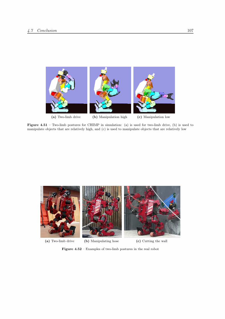
4.7 Conclusion 107
(a) Two-limb drive (b) Manipulation high (c) Manipulation low
Figure 4.51 – Two-limb postures for CHIMP in simulation: (a) is used for two-limb drive, (b) is used tomanipulate objects that are relatively high, and (c) is used to manipulate objects that are relatively low
(a) Two-limb drive (b) Manipulating hose (c) Cutting the wall
Figure 4.52 – Examples of two-limb postures in the real robot
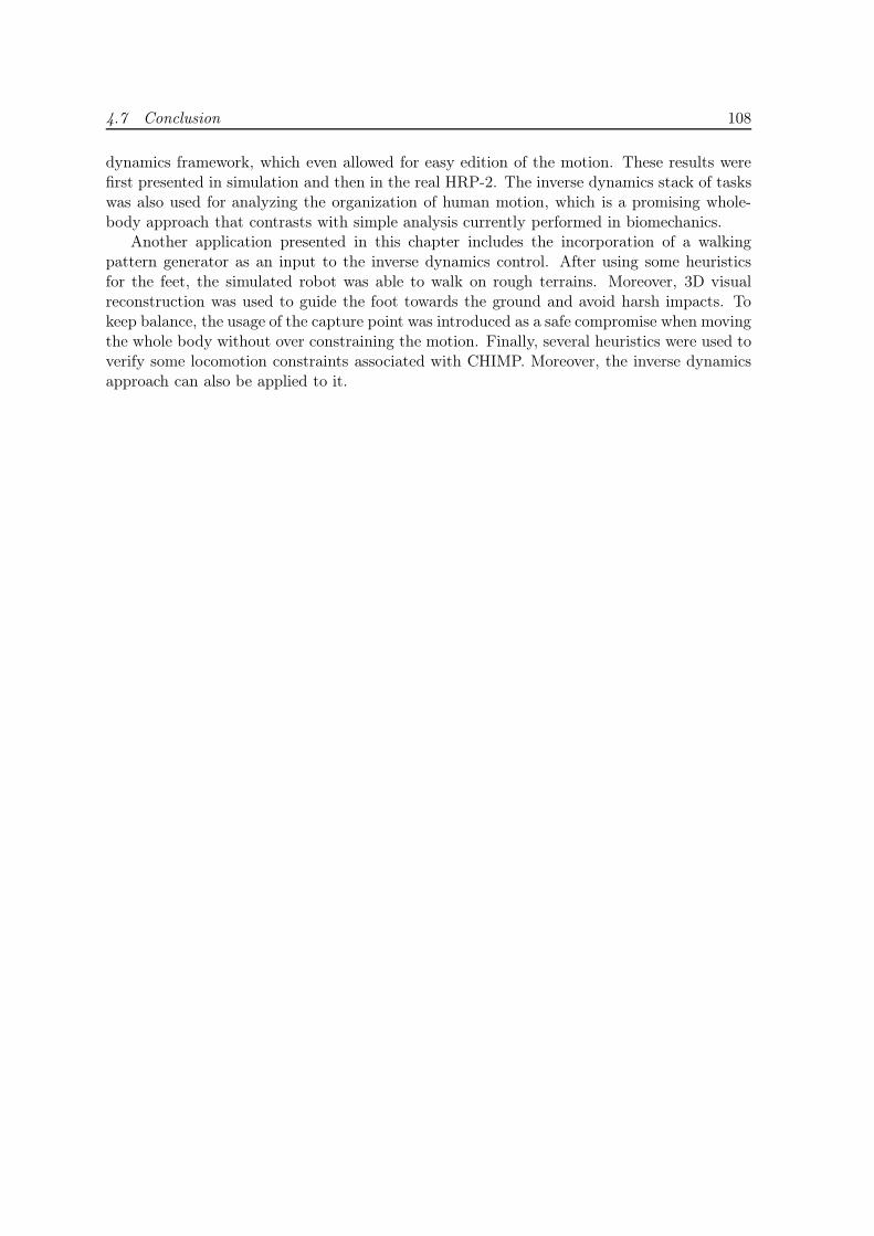
4.7 Conclusion 108
dynamics framework, which even allowed for easy edition of the motion. These results werefirst presented in simulation and then in the real HRP-2. The inverse dynamics stack of taskswas also used for analyzing the organization of human motion, which is a promising whole-body approach that contrasts with simple analysis currently performed in biomechanics.
Another application presented in this chapter includes the incorporation of a walkingpattern generator as an input to the inverse dynamics control. After using some heuristicsfor the feet, the simulated robot was able to walk on rough terrains. Moreover, 3D visualreconstruction was used to guide the foot towards the ground and avoid harsh impacts. Tokeep balance, the usage of the capture point was introduced as a safe compromise when movingthe whole body without over constraining the motion. Finally, several heuristics were used toverify some locomotion constraints associated with CHIMP. Moreover, the inverse dynamicsapproach can also be applied to it.
Chapter 5
Conclusion
The complete operational-space inverse-dynamics control scheme based on the task-functionapproach has been used in this thesis to generate dynamically feasible whole-body motion forhumanoid robots achieving complex behaviors. Several applications showing the effectivenessof the approach have been presented and discussed.
5.1 Contributions
This thesis extended the usage of the operational-space inverse-dynamics control by addingseveral tasks to control the whole robot body. These tasks were formulated in terms ofequalities and inequalities taking advantage of the capability of the control to use them atany level of the hierarchy. Equality tasks were used when a specific point in a certain spaceneeded to be achieved, such as the pose of an operational point (or some components of it)within strict time constraints, or the position of a point in the visual space of the camera.Inequality tasks were used when some quantity needed to be bounded for the motion to befeasible, for instance, joint position and velocity within certain mechanically imposed limitsor the center-of-mass velocity, through the control of the capture point.
The effectiveness of the task-function approach has been demonstrated by generatingdifferent types of motions. The multi-contact capabilities of the control scheme were profitedto make HRP-2 sit in an armchair using a set of tasks knowing the model of the armchair andthe robot, and extensions to other robot or chair models is straightforward. The model ofRomeo was also used to make the robot climb up a ladder by adding and removing tasks andcontacts at the hands and feet sequentially. This thesis also achieved human motion imitationbased on two very efficient tools: motion capture, and the inverse dynamics control. Motioncapture has shown to be a very efficient tool for motion generation when combined with thestack of tasks giving more expressiveness to the motion. The SoT control scheme enforcedthe dynamics of the retargeted motion enabling it to fit with the constraints of the real robot,which are different to those of the human demonstrator. This retargeting approach allowedfor the quick and efficient generation of a long sequence of movements for HRP-2 including
5.2 Perspectives 110
motion in single support such as the yoga figure, fast motion in double support, and arbitrarymotion of the arms while walking. Moreover, the SoT provides some easy edition capabilitiesto correct the defects of the targeted motion or to augment the original movement with someartificial features. Using this framework, the work done in this thesis also found that theSoT can be used as a tool to infer the dynamic organization of human motion preserving keyfeatures of the human motor control organization.
This thesis also achieved walking steps on rough terrain by detecting collision points withstereo vision reconstruction and moving the foot properly to reach a large support polygon,which is equivalent to foot-land compliance. The approach provides a powerful reactive nav-igation system able to deal with a large set of uneven grounds thanks to the efficient inversedynamics setup and the automatic way of finding footsteps. In fact, the only input to thesystem is the direction of motion and the rest is automatically handled by the framework. Themethod was limited to horizontal rough surfaces due to the assumptions of the underlyingwalking pattern generator, but if a different pattern generator is used, the same approachwould be valid for surfaces with different slopes. This thesis also presented the incorporationof the capture point inside the inverse dynamics control through the generation of a dedicatedtask which can bound the velocity of the center of mass. In case a task, or a set of tasks,leads the robot to positions that risk its balance, the capture point task can in principle helpthe balance to be kept and then a step can be automatically launched to avoid falling down.However, this step needs to be very fast, but it is the way a human would react when suddenlylosing balance.
Some movements to generate posture changes for CHIMP were also introduced in thisthesis. The heuristic posture change from having four limbs on the ground to only having twolimbs on the ground was experimentally verified in the robot. Since the robot can move usingits tracks, but keeping its whole body in a pre-determined posture, bounds to the linear andangular velocity as well as linear acceleration were determined and applied to avoid fallingdown when suddenly de-energizing the motors (which was a design requirement). A stabilitycriterion for more generic support polygons, such as the ones found when CHIMP has alltracks on the ground was established as the minimum distance to the edges. It was statedthat the best possible position for the center of mass would be the point that maximizes theminimum distance to the edge of the support polygon. Finally, the inverse dynamics SoT wasapplied to CHIMP allowing the robot to climb the first rung of a ladder.
5.2 Perspectives
On a short term basis, some practical adjustments can be considered. The inverse dynamicscontrol is currently used to generate the desired acceleration and torque to be applied to thesystem, but the control applied to HRP-2 is the position obtained by double integration ofthe acceleration without sensor feedback. The first short term perspective is to apply theinverse dynamics control in closed loop to the robot, modeling the motors of HRP-2 andapplying a torque-like control, or acceleration-like control with sensor feedback. Previouslythis was not achievable due to the computation times but currently the computation timeis real-time at 200Hz and the implementation is only constrained by the technological limitscurrently imposed by the robot. A second perspective in short term is to use a differentwalking pattern generator scheme to allow for applying the software compliant-foot motion
5.2 Perspectives 111
in not only horizontal terrains but with a different slope. A third perspective is to furtherinvestigate the capture point integration in the control scheme, mainly by determining if itwould be efficient to apply it for more than one step or a walking scheme would be moreadequate in that case.
On a middle term basis, an artificial skin can be added to the sole of HRP-2 to effectivelymeasure the position of the contact points and the corresponding contact force. Then, theapproach developed in this thesis in simulation can be directly applied to the real robot. Asecond perspective is to integrate the kinect to the environment sensing. Alternatively, a lidarcan be to scan the 3D environment since it does not depend on lighting conditions as the robotstereo-pair does, and can thus be used for a wide range of environments. The measurementscan be fused with the information obtained from the stereo-pair to have a more robust andmeaningful environmental reconstruction.
Finally, a long term objective would be to find a way to automatically generate the stackof tasks from high level objectives or from the direct observation of human movements. Thisvery challenging objective, that would allow to remove the roboticist form the loop, requires tobe able to automatically structure the observed motion into tasks and constraints, introducinga semantic of the anthropomorphic movement. In this quest, the understanding of the humanmovement will certainly provide engineers with key elements that are still to be discovered.

Appendices
112
Appendix A
Generalized Inverses
A.1 Generalized Inverse
Let A be a matrix in Rm×n. A generalized inverse of A is a matrix A#
g ∈ Rn×m that satisfies
the following condition:AA#
g A = A
which is also called the first Moore-Penrose condition [BenIsrael 03]. A reflexive generalized
inverse of A is a matrix A#r ∈ R
n×m that satisfies
AA#r A = A and A#
r AA#r = A#
r ,
which are also known as the two first conditions of Moore-Penrose. In this document, asstated in Section 3.2.1, A# denotes any reflexive generalized inverse of A.
Properties
1. ∀A ∈ Rm×n ∃A#
g ∈ Rn×m, and ρ(A#
g ) ≥ ρ(A), where ρ(A) denotes the rank of A.
2. A#g = A#
r ⇔ ρ(A#g ) = ρ(A).
3. AA#g = (AA#
g )2 and A#g A = (A#
g A)2.
4. If A is square and non-singular, then, A#g and A#
r are unique and A#g = A#
r = A−1.
5. Let the sets of A#g , and A#
r be S#g and S#
r , respectively, then, S#r ⊂ S#
g . Equivalently,any reflexive generalized inverse is a generalized inverse.
A.2 Pseudo-Inverse 114
A.2 Pseudo-Inverse
The pseudo-inverse, also called the Moore-Penrose inverse of a matrix A ∈ Rm×n is a matrix
A+ ∈ Rn×m satisfying the four Moore-Penrose conditions [Penrose 55]:
AA+A = A (AA+)T = AA+
A+AA+ = A+ (A+A)T = A+A
For particular cases, the pseudo-inverse A+ of A ∈ Rm×n is given by:
• if m < n and ρ(A) = m, then AAT is nonsingular and A+ = AT (AAT )−1,
• if n < m and ρ(A) = n, then ATA is nonsingular and A+ = (ATA)−1AT ,
• if m = n = ρ(A), then A+ = A−1,
• if ATA = I (the columns are orthonormal), or AAT = I (the rows are orthonormal),then A+ = AT .
Properties
1. ∀A ∈ Rm×n, A+ is unique.
2. (AT )+ = (A+)T .
3. A = (A+)+ = (AA+)TA = A(A+A)T .
4. A+ = (ATA)+AT = AT (AAT )+ = A+(AA+)T = (A+A)TA+.
5. The matrices A+A, AA+, I −A+A, and I −AA+ are symmetric and idempotent.
6. If A = AT ∈ Rn×n and A2 = A, then ∀B ∈ R
m×n, A(BA)+ = (BA)+.
7. Given A ∈ Rm×n and B ∈ R
n×p, if (i) ATA = I, or (ii) BBT = I, or (iii) A is fullcolumn rank and B is full row rank, then (AB)+ = B+A+.
Relation with Linear Systems
Let A ∈ Rm×n, x ∈ R
n and b ∈ Rm. The problem of finding the general solution to the linear
system Ax = b, which can be expressed as the minimization problem
minx
‖Ax− b‖22
is given by x∗ = A+b+(I −A+A)z, where z ∈ Rn is an arbitrary vector and ‖.‖2 denotes the
L2 norm of a vector. If additionally, the norm of x has to be minimized; that is,
minx
{‖x‖22 such that x = argmin ‖Ax− b‖22},
the result is given by x∗ = A+b, which is also known as the minimum norm solution.
A.2 Pseudo-Inverse 115
Computation
An efficient way to compute the pseudo-inverse is using the singular value decomposition(SVD). The SVD decomposition of A ∈ R
m×n, with rank ρ(A) = r, is:
A = UΣV T
where U ∈ Rm×m, V ∈ R
n×n are orthogonal matrices (UT = U−1, V T = V −1), and Σ ∈ Rm×n
is a diagonal matrix containing the singular values σi ∈ R of A and zeroes in the diagonal.The form of this matrix is
Σ =
[
Σ 0a0b 0c
]
where Σ =
σ1 0 · · · 00 σ2 · · · 0...
.... . .
...0 0 · · · σr
∈ Rr×r,
0i, with i = {a, b, c}, are zero-matrices such that 0a ∈ Rr×(n−r), 0b ∈ R
(m−r)×r and 0c ∈R(m−r)×(n−r), and σ1 ≥ σ2 ≥ . . . ≥ σr ≥ 0. Let ui ∈ R
m and vi ∈ Rn represent the ith
columns of U and V , respectively, so that
U =[
u1 · · · ur ur+1 · · · um]
V =[
v1 · · · vr vr+1 · · · vn]
.
The vectors ui, vi are the ith left and right singular vectors of A, respectively, satisfyingAvi = σiui and ATui = σivi, for i = 1, · · · , r. An orthonormal basis for the image of A isthe set {u1, · · · , ur}, and an orthonormal basis for the kernel of A is the set {vr+1, · · · , vn}.Considering only the first r vectors, A can be reduced to:
A =
r∑
i=1
σiuivTi
Since the matrix Σ is diagonal, its inverse Σ−1 can be obtained replacing σi by σ−1i . Then,
the computation of A+ is directly:
A+ = V Σ−1UT = V
[
Σ−1 0a0b 0c
]
UT =r∑
i=1
1
σiviu
Ti
In cases where σi → 0, the denominator might be ill-defined. In these cases, the dampedpseudo-inverse A† can be used, and is computed as
A† =r∑
i=1
σiσ2i + α2
viuTi
where α is the damping factor. The damped pseudo-inverse is the solution x∗ = A†b to theproblem
minx
‖Ax− b‖22 + α2‖x‖22
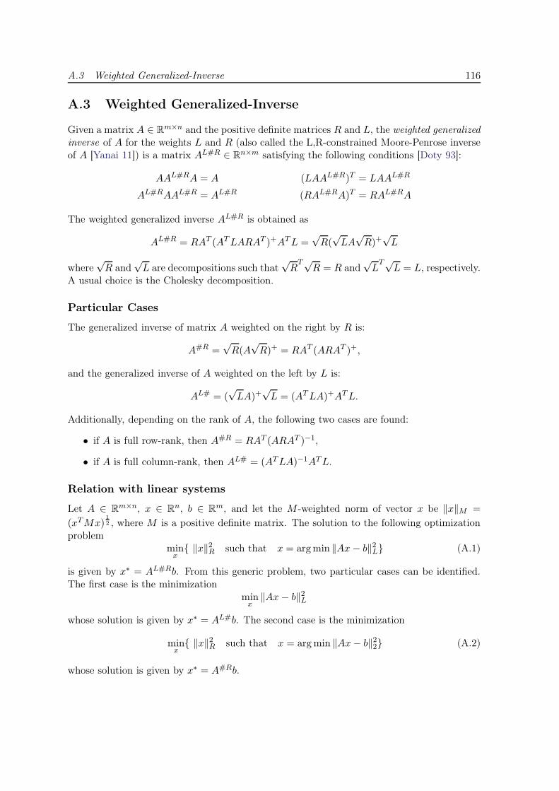
A.3 Weighted Generalized-Inverse 116
A.3 Weighted Generalized-Inverse
Given a matrix A ∈ Rm×n and the positive definite matrices R and L, the weighted generalized
inverse of A for the weights L and R (also called the L,R-constrained Moore-Penrose inverseof A [Yanai 11]) is a matrix AL#R ∈ R
n×m satisfying the following conditions [Doty 93]:
AAL#RA = A (LAAL#R)T = LAAL#R
AL#RAAL#R = AL#R (RAL#RA)T = RAL#RA
The weighted generalized inverse AL#R is obtained as
AL#R = RAT (ATLARAT )+ATL =√R(
√LA
√R)+
√L
where√R and
√L are decompositions such that
√RT√
R = R and√LT√
L = L, respectively.A usual choice is the Cholesky decomposition.
Particular Cases
The generalized inverse of matrix A weighted on the right by R is:
A#R =√R(A
√R)+ = RAT (ARAT )+,
and the generalized inverse of A weighted on the left by L is:
AL# = (√LA)+
√L = (ATLA)+ATL.
Additionally, depending on the rank of A, the following two cases are found:
• if A is full row-rank, then A#R = RAT (ARAT )−1,
• if A is full column-rank, then AL# = (ATLA)−1ATL.
Relation with linear systems
Let A ∈ Rm×n, x ∈ R
n, b ∈ Rm, and let the M -weighted norm of vector x be ‖x‖M =
(xTMx)1
2 , where M is a positive definite matrix. The solution to the following optimizationproblem
minx
{ ‖x‖2R such that x = argmin ‖Ax− b‖2L} (A.1)
is given by x∗ = AL#Rb. From this generic problem, two particular cases can be identified.The first case is the minimization
minx
‖Ax− b‖2L
whose solution is given by x∗ = AL#b. The second case is the minimization
minx
{ ‖x‖2R such that x = argmin ‖Ax− b‖22} (A.2)
whose solution is given by x∗ = A#Rb.
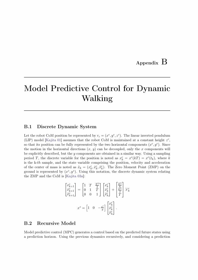
Appendix B
Model Predictive Control for Dynamic
Walking
B.1 Discrete Dynamic System
Let the robot CoM position be represented by rc = (xc, yc, zc). The linear inverted pendulum(LIP) model [Kajita 01] assumes that the robot CoM is maintained at a constant height zc,so that its position can be fully represented by the two horizontal components (xc, yc). Sincethe motion in the horizontal directions (x, y) can be decoupled, only the x components willbe explicitly described, but the y components are obtained in a similar way. Using a samplingperiod T , the discrete variable for the position is noted as xck = xc(kT ) = xc(tk), where kis the k-th sample, and the state variable comprising the position, velocity and accelerationof the center of mass is noted as xk = (xck, x
ck, x
ck). The Zero Moment Point (ZMP) on the
ground is represented by (xz, yz). Using this notation, the discrete dynamic system relatingthe ZMP and the CoM is [Kajita 03a]:
xck+1
xck+1
xck+1
=
1 T T 2
20 1 T0 0 1
xckxckxck
+
T 3
6T 2
2T
...x ck
xz =[
1 0 − zc
g
]
xckxckxck
.
B.2 Recursive Model
Model predictive control (MPC) generates a control based on the predicted future states usinga prediction horizon. Using the previous dynamics recursively, and considering a prediction
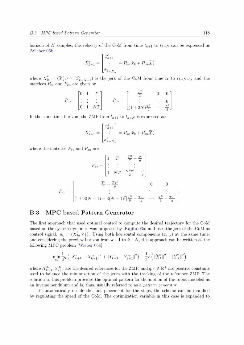
B.3 MPC based Pattern Generator 118
horizon of N samples, the velocity of the CoM from time tk+1 to tk+N can be expressed as[Wieber 06b]:
Xck+1 =
xck+1...
xck+N
= Pvs xk + Pvu
...Xck
where...Xck = (
...x ck, · · · ,
...x ck+N−1) is the jerk of the CoM from time tk to tk+N−1, and the
matrices Pvs and Pvu are given by
Pvs =
0 1 T...
......
0 1 NT
Pvu =
T 2
2 0 0...
. . . 0
(1 + 2N)T2
2 · · · T 2
2
.
In the same time horizon, the ZMP from tk+1 to tk+N is expressed as:
Xzk+1 =
xzk+1...
xzk+N
= Pzs xk + Pzu
...Xck
where the matrices Pzs and Pzu are
Pzs =
1 T T 2
2 − zc
g...
......
1 NT N2T 2
2 − zc
g
Pzu =
T 3
6 − Tzc
g0 0
.... . .
...[1 + 3(N − 1) + 3(N − 1)2]T
3
6 − Tzc
g· · · T 3
6 − Tzc
g
.
B.3 MPC based Pattern Generator
The first approach that used optimal control to compute the desired trajectory for the CoMbased on the system dynamics was proposed by [Kajita 03a] and uses the jerk of the CoM ascontrol signal: uk = (
...Xck,
...Yck). Using both horizontal components (x, y) at the same time,
and considering the preview horizon from k+1 to k+N , this approach can be written as thefollowing MPC problem [Wieber 06b]:
minuk
1
2q(
‖Xzk+1 −Xzr
k+1‖2 + ‖Y zk+1 − Y zr
k+1‖2)
+1
2r(
‖...Xck‖2 + ‖ ...
Yck‖2)
where Xzrk+1, Y
zrk+1 are the desired references for the ZMP, and q, r ∈ R
+ are positive constantsused to balance the minimization of the jerks with the tracking of the reference ZMP. Thesolution to this problem provides the optimal pattern for the motion of the robot modeled asan inverse pendulum and is, thus, usually referred to as a pattern generator.
To automatically decide the foot placement for the steps, the scheme can be modifiedby regulating the speed of the CoM. The optimization variable in this case is expanded to
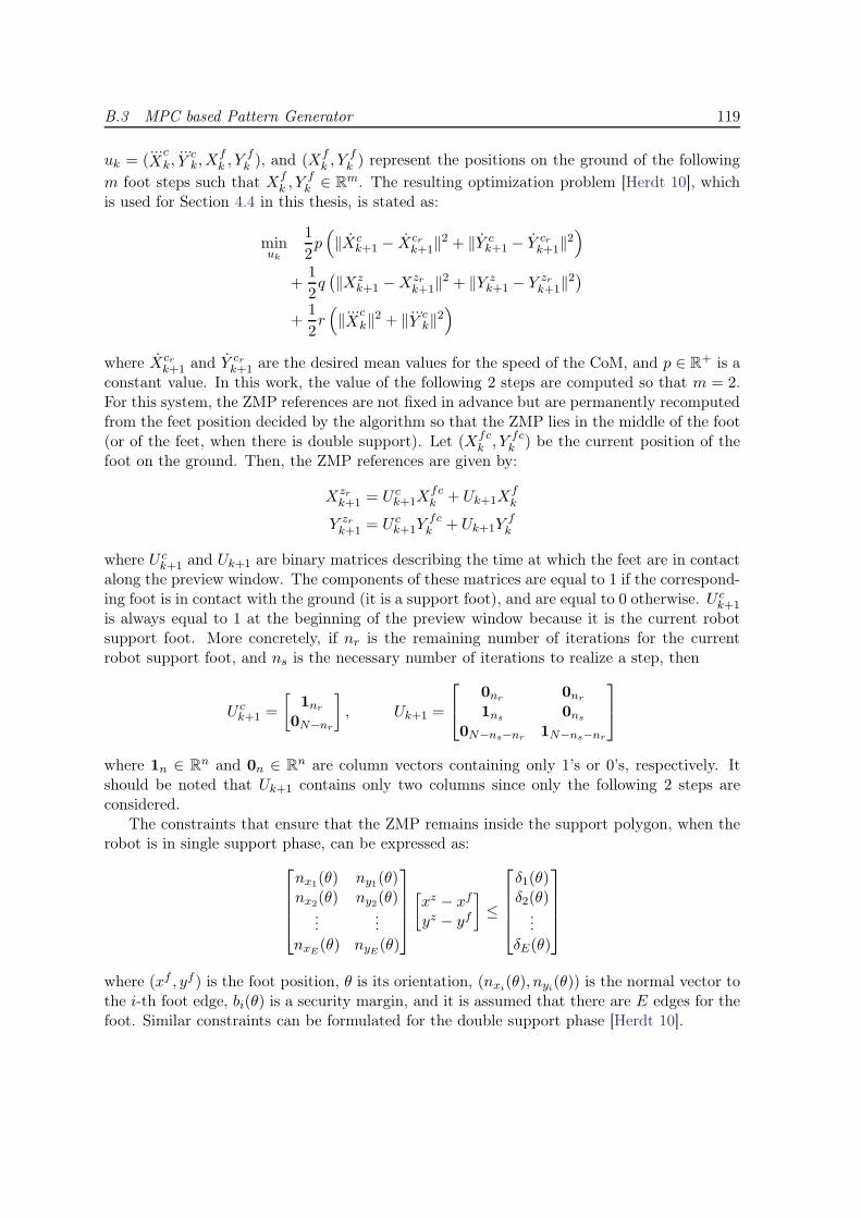
B.3 MPC based Pattern Generator 119
uk = (...Xck,
...Yck,X
fk , Y
fk ), and (Xf
k , Yfk ) represent the positions on the ground of the following
m foot steps such that Xfk , Y
fk ∈ R
m. The resulting optimization problem [Herdt 10], whichis used for Section 4.4 in this thesis, is stated as:
minuk
1
2p(
‖Xck+1 − Xcr
k+1‖2 + ‖Y ck+1 − Y cr
k+1‖2)
+1
2q(
‖Xzk+1 −Xzr
k+1‖2 + ‖Y zk+1 − Y zr
k+1‖2)
+1
2r(
‖...Xck‖2 + ‖ ...
Yck‖2)
where Xcrk+1 and Y cr
k+1 are the desired mean values for the speed of the CoM, and p ∈ R+ is a
constant value. In this work, the value of the following 2 steps are computed so that m = 2.For this system, the ZMP references are not fixed in advance but are permanently recomputedfrom the feet position decided by the algorithm so that the ZMP lies in the middle of the foot(or of the feet, when there is double support). Let (Xfc
k , Yfck ) be the current position of the
foot on the ground. Then, the ZMP references are given by:
Xzrk+1 = U ck+1X
fck + Uk+1X
fk
Y zrk+1 = U ck+1Y
fck + Uk+1Y
fk
where U ck+1 and Uk+1 are binary matrices describing the time at which the feet are in contactalong the preview window. The components of these matrices are equal to 1 if the correspond-ing foot is in contact with the ground (it is a support foot), and are equal to 0 otherwise. U ck+1
is always equal to 1 at the beginning of the preview window because it is the current robotsupport foot. More concretely, if nr is the remaining number of iterations for the currentrobot support foot, and ns is the necessary number of iterations to realize a step, then
U ck+1 =
[
1nr
0N−nr
]
, Uk+1 =
0nr 0nr
1ns 0ns
0N−ns−nr 1N−ns−nr
where 1n ∈ Rn and 0n ∈ R
n are column vectors containing only 1’s or 0’s, respectively. Itshould be noted that Uk+1 contains only two columns since only the following 2 steps areconsidered.
The constraints that ensure that the ZMP remains inside the support polygon, when therobot is in single support phase, can be expressed as:
nx1(θ) ny1(θ)nx2(θ) ny2(θ)
......
nxE(θ) nyE(θ)
[
xz − xf
yz − yf
]
≤
δ1(θ)δ2(θ)
...δE(θ)
where (xf , yf ) is the foot position, θ is its orientation, (nxi(θ), nyi(θ)) is the normal vector tothe i-th foot edge, bi(θ) is a security margin, and it is assumed that there are E edges for thefoot. Similar constraints can be formulated for the double support phase [Herdt 10].
Appendix C
Capture Point
This Appendix gives a brief review of the derivation of the Capture Point, which is used forthe Capture Point task throughout this document.
C.1 Linear Inverted Pendulum (LIP)
The linear inverted pendulum (LIP), described in [Kajita 01], can be used as a model for theanalysis of a humanoid robot in the space. It consists in approximating the dynamics of therobot by an inverted pendulum according to some assumptions, which are the following.
1. The robot is represented by a punctual mass m located at its center of mass (CoM).
2. The legs of the robot are massless and the extreme in contact with the ground can befreely moved (it is not externally actuated).
3. The height of the CoM is kept constant throughout the motion.
Consider the LIP model shown in Fig. C.1. Let the position of the CoM be represented byrc = (xc, yc, zc), the point of the pendulum in contact with the ground by rz = (xz, yz, 0), andthe force that acts along the pendulum by F = (fx, fy, fz). For a robot with feet, the pointrz is equivalent to the Center-of-Pressure (CoP), which is equivalent to the ZMP of the robot[Sardain 04]. With this notation, the equations of motion for the system are:
mrc = F +mG (C.1)
(rc − rz)×F = 0 (C.2)
where G = (0, 0,−g) is the gravity vector.Since the third assumptions of the model implies a continuous constant height for the
CoM (zc = 0), then, both the velocity and the acceleration of the CoM will have a null thirdcomponent: zc = zc = 0. With this consideration, the components of (C.1) can be written as
fx = mxc, fy = myc, fz = mg. (C.3)
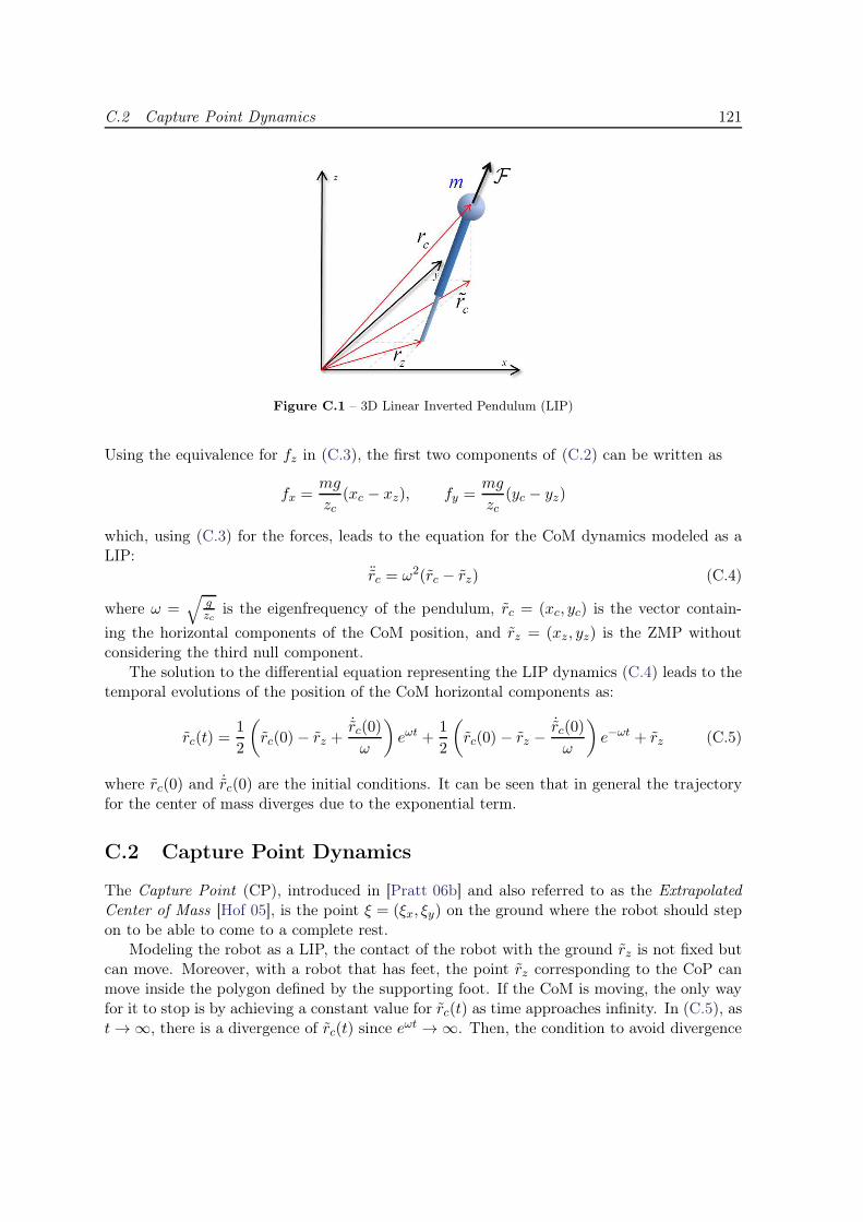
C.2 Capture Point Dynamics 121
Figure C.1 – 3D Linear Inverted Pendulum (LIP)
Using the equivalence for fz in (C.3), the first two components of (C.2) can be written as
fx =mg
zc(xc − xz), fy =
mg
zc(yc − yz)
which, using (C.3) for the forces, leads to the equation for the CoM dynamics modeled as aLIP:
¨rc = ω2(rc − rz) (C.4)
where ω =√
gzc
is the eigenfrequency of the pendulum, rc = (xc, yc) is the vector contain-
ing the horizontal components of the CoM position, and rz = (xz, yz) is the ZMP withoutconsidering the third null component.
The solution to the differential equation representing the LIP dynamics (C.4) leads to thetemporal evolutions of the position of the CoM horizontal components as:
rc(t) =1
2
(
rc(0)− rz +˙rc(0)
ω
)
eωt +1
2
(
rc(0) − rz −˙rc(0)
ω
)
e−ωt + rz (C.5)
where rc(0) and ˙rc(0) are the initial conditions. It can be seen that in general the trajectoryfor the center of mass diverges due to the exponential term.
C.2 Capture Point Dynamics
The Capture Point (CP), introduced in [Pratt 06b] and also referred to as the ExtrapolatedCenter of Mass [Hof 05], is the point ξ = (ξx, ξy) on the ground where the robot should stepon to be able to come to a complete rest.
Modeling the robot as a LIP, the contact of the robot with the ground rz is not fixed butcan move. Moreover, with a robot that has feet, the point rz corresponding to the CoP canmove inside the polygon defined by the supporting foot. If the CoM is moving, the only wayfor it to stop is by achieving a constant value for rc(t) as time approaches infinity. In (C.5), ast→ ∞, there is a divergence of rc(t) since eωt → ∞. Then, the condition to avoid divergence
C.2 Capture Point Dynamics 122
is that the coefficient of the exponential be null, that is:
rc(0) +˙rc(0)
ω= rz. (C.6)
Using the condition (C.6), the limit for the CoM position (C.5) and for its velocity, which canbe easily shown, as time approaches infinity is
limt→∞
{rc(t)} = rz = ξ
limt→∞
{ ˙rc(t)} = 0
where ξ is called the Capture Point since it is the only point where the CoM can come to arest. Considering this equivalence for ξ, the condition (C.6) for a general position of the CoMgives the expression for the instantaneous capture point as:
ξ = rc +˙rcω
(C.7)
It is also possible to find the expression of the instantaneous capture point by analyzing theorbital energy of the pendulum [Pratt 06a].
The velocity of the capture point can be obtained by differentiating (C.7) and replacingboth (C.4) and the expression for the velocity of the CoM from (C.7), and is given by:
ξ = ω(ξ − rz) (C.8)
This expression represents the first order dynamics of the CP. Solving the differential equation(C.8), the explicit formulation of the instantaneous capture point trajectory as a function oftime is
ξ(t) = (ξ0 − rz)eωt + rz (C.9)
where ξ0 is ξ at the initial time t0. The computation of (C.9) allows a prediction of the futureposition of the capture point.
Bibliography
[Abe 07] Y. Abe, M. da Silva, J. Popović. – Multiobjective control with frictional contacts. –ACM SIGGRAPH/Eurographics symposium on Computer Animation, 2007.
[Abry 97] P. Abry. – Ondelettes et turbulence, Multirésolutions, algorithmes de décomposition,invariance d’échelles. – Diderot Editeur, Paris, 1997.
[Aghili 05] F. Aghili. – A unified approach for inverse and direct dynamics of constrained multibodysystems based on linear projection operator: applications to control and simulation. IEEETransactions on Robotics (TRO), 21(5):834–849, 2005.
[AlAzemi 13] H. Al-Azemi. – Fire fighting robot, February 2013. US Patent 8,381,826.
[AlBorno 13] M. Al Borno, M. de Lasa, A. Hertzmann. – Trajectory optimization for full-body move-ments with complex contacts. IEEE Transactions on Visualization and Computer Graph-ics, 19(8):1405–1414, 2013.
[AlBorno 14] M. Al Borno, E. Fiume, A. Hertzmann, M. de Lasa. – Feedback control for rotationalmovements in feature space. ACM SIGGRAPH/Eurographics Symposium on ComputerAnimation, 2014.
[Ali 10] M. Ali, H. Park, C.S. Lee. – Closed-form inverse kinematic joint solution for humanoidrobots. – IEEE/RSJ International Conference on Intelligent Robots and Systems (IROS),2010.
[Ambrose 04] R. O Ambrose, R. T Savely, S. Goza, P. Strawser, M. Diftler, I. Spain, N. Radford.– Mobile manipulation using nasa’s robonaut. – IEEE International Confenrence onRobotics and Automation (ICRA), 2004.
[Arbulu 07] M. Arbulu, C. Balaguer. – Real-time gait planning for rh-1 humanoid robot, usinglocal axis gait algorithm. – IEEE/RAS International Conference on Humanoid Robots(Humanoids), 2007.
[Arimoto 83] S. Arimoto, F. Miyazaki. – Stability and robustness of pid feedback control for robotmanipulators of sensory capability. – Robotics Research, 1st International Symposium,1983.
[Arisumi 08] H. Arisumi, S. Miossec, J-R Chardonnet, K. Yokoi. – Dynamic lifting by whole bodymotion of humanoid robots. – IEEE/RSJ International Conference on Intelligent Robotsand Systems (IROS), 2008.
[Arnol’d 89] V.I. Arnol’d. – Mathematical methods of classical mechanics. – Springer, vol. 60, 1989.
[Asfour 06] T. Asfour, K. Regenstein, P. Azad, J. Schroder, A. Bierbaum, N. Vahrenkamp, R. Dill-mann. – Armar-iii: An integrated humanoid platform for sensory-motor control. –IEEE/RAS International Conference on Humanoid Robots (Humanoids), 2006.
[Atkeson 94] C.G. Atkeson. – Using local trajectory optimizers to speed up global optimization indynamic programming. Advances in Neural Information Processing Systems, pp. 663–670, 1994.
Bibliography 124
[Atkeson 00] C.G. Atkeson, J. Hale, F. Pollick, M. Riley, S. Kotosaka, S. Schaul, T. Shibata, G. Teva-tia, A. Ude, S. Vijayakumar. – Using humanoid robots to study human behavior. IEEEIntelligent Systems and their applications, 15(4):46–56, 2000.
[Atkeson 03] C.G. Atkeson, J. Morimoto. – Nonparametric representation of policies and value func-tions: A trajectory-based approach. Advances in Neural Information Processing Systems,15, 2003.
[Ayaz 07] Y. Ayaz, K. Munawar, M. Malik, A. Konno, M. Uchiyama. – Human-like approach tofootstep planning among obstacles for humanoid robots. International Journal of Hu-manoid Robotics (IJHR), 4(01):125–149, 2007.
[Baerlocher 98] P. Baerlocher, R. Boulic. – Task-priority formulations for the kinematic control of highlyredundant articulated structures. – IEEE/RSJ International Conference on IntelligentRobots and Systems (IROS), 1998.
[Baerlocher 04] P. Baerlocher, R. Boulic. – An inverse kinematics architecture enforcing an arbitrarynumber of strict priority levels. The visual computer, 20(6):402–417, 2004.
[Baillieul 85] J. Baillieul. – Kinematic programming alternatives for redundant manipulators. – IEEEInternational Confenrence on Robotics and Automation (ICRA), 1985.
[Baillieul 90] J. Baillieul, D.P. Martin. – Resolution of kinematic redundancy. – Proceedings of Sym-posia in Applied Mathematics, 1990.
[Bejczy 74] A.K. Bejczy. – Robot arm dynamics and control, 1974.
[Bellman 56] R. Bellman. – Dynamic programming and lagrange multipliers. Proceedings of the Na-tional Academy of Sciences of the United States of America, 42(10):767, 1956.
[BenIsrael 03] A. Ben-Israel, T.N.E. Greville. – Generalized inverses: Theory and applications. –Springer, 2003.
[Berenson 11] D. Berenson, S.S. Srinivasa, J. Kuffner. – Task Space Regions: A framework forpose-constrained manipulation planning. The International Journal of Robotics Research(IJRR), 2011.
[Bouyarmane 11] K. Bouyarmane, A. Kheddar. – Using a multi-objective controller to synthesize simulatedhumanoid robot motion with changing contact configurations. – IEEE/RSJ InternationalConference on Intelligent Robots and Systems (IROS), 2011.
[Bouyarmane 12a] K. Bouyarmane, A. Kheddar. – Humanoid robot locomotion and manipulation stepplanning. Advanced Robotics, 26(10):1099–1126, 2012.
[Bouyarmane 12b] K. Bouyarmane, A. Kheddar. – On the dynamics modeling of free-floating-base artic-ulated mechanisms and applications to humanoid whole-body dynamics and control. –IEEE/RAS International Conference on Humanoid Robots (Humanoids), 2012.
[Bretl 06] T. Bretl. – Motion planning of multi-limbed robots subject to equilibrium constraints:The free-climbing robot problem. The International Journal of Robotics Research (IJRR),25(4):317–342, 2006.
[Brown 13] D. Brown, A. Macchietto, K. Yin, V. Zordan. – Control of rotational dynamics for groundbehaviors. – ACM SIGGRAPH/Eurographics Symposium on Computer Animation, 2013.
[Caccavale 98] F. Caccavale, C. Natale, B. Siciliano, L. Villani. – Resolved-acceleration control of robotmanipulators: A critical review with experiments. Robotica, 16(05):565–573, 1998.
[Calinon 07] S. Calinon, F. Guenter, A. Billard. – On learning, representing, and generalizing a task ina humanoid robot. IEEE Transactions on Systems, Man and Cybernetics, 37(2):286–298,2007.
[Canny 88] J. Canny. – The complexity of robot motion planning. – The MIT Press, 1988.
[Capek 20] K. Capek, N. Playfair, P. Selver, WA. Landes. – Rossum’s universal robots. – Prague,CZ, 1920.
[Chang 08] Y. Chang, Y. Oh, D. Kim, S. Hong. – Balance control in whole body coordination frame-work for biped humanoid robot mahru-r. – The 17th IEEE International Symposium onRobot and Human Interactive Communication, 2008.
Bibliography 125
[Chaumette 06] F. Chaumette, S. Hutchinson. – Visual servo control. I. Basic approaches. IEEE Robotics& Automation Magazine (RAM), 13(4):82–90, 2006.
[Cheng 07] G. Cheng, S. Hyon, J. Morimoto, A. Ude, J. Hale, G. Colvin, W. Scroggin, S. Jacobsen.– Cb: A humanoid research platform for exploring neuroscience. Advanced Robotics,21(10):1097–1114, 2007.
[Chestnutt 05] J. Chestnutt, M. Lau, G. Cheung, J. Kuffner, J. Hodgins, T. Kanade. – Footstep planningfor the honda asimo humanoid. – IEEE International Confenrence on Robotics andAutomation (ICRA), 2005.
[Choset 05] H. Choset, K.M. Lynch, S. Hutchinson, G.A. Kantor, W. Burgard, L.E. Kavraki,S. Thrun. – Principles of Robot Motion: theory, algorithms, and implementation. –MIT Press, 2005.
[Coleman 00] R. Coleman. – Multi-feature automated wheelchair, November 2000. US Patent6,154,690.
[Collette 08] C. Collette, A. Micaelli, C. Andriot, P. Lemerle. – Robust balance optimization controlof humanoid robots with multiple non coplanar grasps and frictional contacts. – IEEEInternational Confenrence on Robotics and Automation (ICRA), 2008.
[Craig 89] J.J. Craig. – Introduction to robotics. – Addison-Wesley Reading, MA, vol. 7, 1989.
[Dalibard 13] S. Dalibard, A. El Khoury, F. Lamiraux, A. Nakhaei, M. Taïx, J-P. Laumond. – Dynamicwalking and whole-body motion planning for humanoid robots: an integrated approach.The International Journal of Robotics Research (IJRR), 2013.
[Dariush 10] B. Dariush, G. Hammam, D. Orin. – Constrained resolved acceleration control forhumanoids. – IEEE/RSJ International Conference on Intelligent Robots and Systems(IROS), 2010.
[DaSilva 08] M. Da Silva, Y. Abe, J. Popović. – Simulation of human motion data using short-horizonmodel-predictive control. – Computer Graphics Forum, 2008.
[deLasa 10] M. de Lasa, I. Mordatch, A. Hertzmann. – Feature-based locomotion controllers. ACMTransactions on Graphics (SIGGRAPH), 29(3), 2010.
[Dellin 12] C. Dellin, S. Srinivasa. – A framework for extreme locomotion planning. – IEEE Inter-national Confenrence on Robotics and Automation (ICRA), 2012.
[Dellon 07] B. Dellon, Y. Matsuoka. – Prosthetics, exoskeletons, and rehabilitation. IEEE Robotics& Automation Magazine (RAM), 14(1):30–34, 2007.
[DelPrete 14a] A. Del Prete, F. Nori, G. Metta, L. Natale. – Partial force control of constrained floating-base robots. – IEEE International Confenrence on Robotics and Automation (ICRA),2014.
[DelPrete 14b] A. Del Prete, F. Romano, F. Nori, G. Metta, G. Sandini, L. Natale. – Prioritized optimalcontrol. – IEEE International Confenrence on Robotics and Automation (ICRA), 2014.
[Denavit 55] J. Denavit, R. S. Hartenberg. – A kinematic notation for lower-pair mechanisms basedon matrices. ASME Journal of Applied Mechanics, 22:215–221, 1955.
[Dimitrov 11] D. Dimitrov, A. Sherikov, P-B Wieber. – A sparse model predictive control formulationfor walking motion generation. – IEEE/RSJ International Conference on IntelligentRobots and Systems (IROS), 2011.
[Doty 93] K.L. Doty, C. Melchiorri, C. Bonivento. – A theory of generalized inverses applied torobotics. The International Journal of Robotics Research (IJRR), 12(1):1, 1993.
[Dubowsky 79] S. Dubowsky, DT DesForges. – The application of model-referenced adaptive con-trol to robotic manipulators. Journal of Dynamic Systems, Measurement, and Control,101(3):193–200, 1979.
[Durán 12] B. Durán, S. Thill. – Rob’s robot: Current and future challenges for humanoid robots.In The Future of Humanoid Robots-Research and Applications, 2012.
[ElKhoury 13] A. El Khoury, F. Lamiraux, M. Taix. – Optimal motion planning for humanoid robots.– IEEE International Confenrence on Robotics and Automation (ICRA), 2013.
Bibliography 126
[Endo 08] N. Endo, S. Momoki, M. Zecca, M. Saito, Y. Mizoguchi, K. Itoh, A. Takanishi. – De-velopment of whole-body emotion expression humanoid robot. – IEEE InternationalConfenrence on Robotics and Automation (ICRA), 2008.
[Englsberger 11] J. Englsberger, C. Ott, M. Roa, A. Albu-Schaffer, G. Hirzinger. – Bipedal walking controlbased on capture point dynamics. – IEEE/RSJ International Conference on IntelligentRobots and Systems (IROS), 2011.
[Escande 13] A. Escande, A. Kheddar, S. Miossec. – Planning contact points for humanoid robots.Robotics and Autonomous Systems, 2013.
[Escande 14] A. Escande, N. Mansard, P-B. Wieber. – Hierarchical quadratic programming. TheInternational Journal of Robotics Research (IJRR), 2014.
[Everett 87] L. Everett, M. Driels, B.W. Mooring. – Kinematic modelling for robot calibration. –IEEE International Confenrence on Robotics and Automation (ICRA), 1987.
[Featherstone 00] R. Featherstone, D. Orin. – Robot dynamics: Equations and algorithms. – IEEE Inter-national Confenrence on Robotics and Automation (ICRA), 2000.
[Featherstone 08] R. Featherstone. – Rigid body dynamics algorithms. – Springer New York, vol. 49, 2008.
[Fink 12] J. Fink. – Anthropomorphism and human likeness in the design of robots and human-robot interaction. Social Robotics, pp. 199–208. – Springer, 2012.
[Galdeano 14] D. Galdeano, A. Chemori, S. Krut, P. Fraisse. – Task-based whole-body control ofhumanoid robots with zmp regulation, real-time application to a squat-like motion. –SSD SAC 2014: 11th International Conference on Systems, Analysis and AutomaticControl, 2014.
[Geiger 10] M. Geiger, M. Roser, R. Urtasun. – Efficient large-scale stereo matching. – AsianConference on Computer Vision, 2010.
[Geoffroy 14] P. Geoffroy, N. Mansard, M. Raison, S. Achiche, Y. Tassa, E. Todorov. – From inversekinematics to optimal control. Advances in Robot Kinematics, 2014.
[Geppert 04] L. Geppert. – Qrio, the robot that could. IEEE Spectrum, 41(5):34–37, 2004.
[Gienger 05] M. Gienger, H. Janssen, C. Goerick. – Task-oriented whole body motion for humanoidrobots. – IEEE/RAS International Conference on Humanoid Robots (Humanoids), 2005.
[Gleicher 98] M. Gleicher. – Retargetting motion to new characters. – ACM Transactions on Graphics(SIGGRAPH), 1998.
[Gogu 05] G. Gogu. – Chebychev–grübler–kutzbach’s criterion for mobility calculation of multi-loop mechanisms revisited via theory of linear transformations. European Journal ofMechanics-A/Solids, 24(3):427–441, 2005.
[Goodman 04] J.E. Goodman, J. O’Rourke. – Handbook of discrete and computational geometry. – CRCpress, 2004.
[Goswami 99] A. Goswami. – Foot rotation indicator (fri) point: A new gait planning tool to evaluatepostural stability of biped robots. – IEEE International Confenrence on Robotics andAutomation (ICRA), 1999.
[Gottschalk 96] S. Gottschalk, M.C. Lin, D. Manocha. – Obbtree: a hierarchical structure for rapidinterference detection. – Conference on Computer Graphics and Interactive Techniques,1996.
[Gouaillier 09] D. Gouaillier, V. Hugel, P. Blazevic, Ch. Kilner, J. Monceaux, P. Lafourcade, B. Marnier,J. Serre, B. Maisonnier. – Mechatronic design of nao humanoid. – IEEE InternationalConfenrence on Robotics and Automation (ICRA), Kobe, Japan, 2009.
[Grey 13] M. Grey, N. Dantam, D. Lofaro, A. Bobick, M. Egerstedt, P. Oh, M. Stilman. – Multi-process control software for hubo2 plus robot. – IEEE International Conference onTechnologies for Practical Robot Applications (TePRA), 2013.
[Guigon 07] E. Guigon, P. Baraduc, M. Desmurget. – Computational motor control: redundancy andinvariance. Journal of neurophysiology, 97(1):331–347, 2007.
Bibliography 127
[H. 11] Sovannara H. – Reconnaissance de Tâches par Commande Inverse. – PhD. Thesis,University of Toulouse (INSA Toulouse) and LAAS-CNRS, November 2011.
[Hak 12] S. Hak, N. Mansard, O. Stasse, J-P. Laumond. – Reverse control for humanoid robottask recognition. IEEE Transactions on Systems, Man and Cybernetics, 42(6):1524–1537,2012.
[Harmeyer 04] S. Harmeyer, A. Bowling. – Dynamic performance as a criterion for redundant manipu-lator control. – IEEE/RSJ International Conference on Intelligent Robots and Systems(IROS), 2004.
[Hauser 10] K. Hauser, J.C. Latombe. – Multi-modal motion planning in non-expansive spaces. TheInternational Journal of Robotics Research (IJRR), 29(7):897–915, 2010.
[Hayati 85] S. Hayati, M. Mirmirani. – Improving the absolute positioning accuracy of robot manip-ulators. Journal of Robotic Systems, 2(4):397–413, 1985.
[Herdt 10] A. Herdt, H. Diedam, P.B. Wieber, D. Dimitrov, K. Mombaur, M. Diehl. – Onlinewalking motion generation with automatic footstep placement. Advanced Robotics, 24,5(6):719–737, 2010.
[Herzog 13] A. Herzog, L. Righetti, F. Grimminger, P. Pastor, S. Schaal. – Experiments with ahierarchical inverse dynamics controller on a torque-controlled humanoid. arXiv preprint,2013.
[Hirai 98] K. Hirai, M. Hirose, Y. Haikawa, T. Takenaka. – The development of Honda humanoidrobot. – IEEE International Confenrence on Robotics and Automation (ICRA), 1998.
[Hirose 01] R. Hirose, T. Takenaka. – Development of the humanoid robot ASIMO. Honda R&DTechnical Review, 13(1):1–6, 2001.
[Hockstein 07] N. Hockstein, C. Gourin, R. Faust, D. Terris. – A history of robots: from science fictionto surgical robotics. Journal of robotic surgery, 1(2):113–118, 2007.
[Hof 05] A.L. Hof, M. Gazendam, W. Sinke. – The condition for dynamic stability. Journal ofbiomechanics, 38(1):1–8, 2005.
[Hofmann 09] A. Hofmann, M. Popovic, H. Herr. – Exploiting angular momentum to enhance bipedalcenter-of-mass control. – IEEE International Confenrence on Robotics and Automation(ICRA), 2009.
[Hollerbach 80] J.M. Hollerbach. – A recursive lagrangian formulation of maniputator dynamics and acomparative study of dynamics formulation complexity. IEEE Transactions on Systems,Man and Cybernetics, 10(11):730–736, 1980.
[Hornby 00] G. Hornby, S. Takamura, J. Yokono, O. Hanagata, T. Yamamoto, M. Fujita. – Evolvingrobust gaits with aibo. – IEEE International Confenrence on Robotics and Automation(ICRA), 2000.
[Hornung 13] A. Hornung, D. Maier, M. Bennewitz. – Search-based footstep planning. – ICRA - Work-shop on Progress and Open Problems in Motion Planning and Navigation for Humanoids,Karlsruhe, Germany, May 2013.
[Hsu 97] D. Hsu, J-C. Latombe, R. Motwani. – Path planning in expansive configuration spaces.– IEEE International Confenrence on Robotics and Automation (ICRA), 1997.
[Hudson 97] T.C. Hudson, M.C. Lin, J. Cohen, S. Gottschalk, D. Manocha. – V-collide: acceleratedcollision detection for vrml. – Symposium on Virtual Reality Modeling Language, 1997.
[Hunt 67] KH Hunt. – Prismatic pairs in spatial linkages. Journal of Mechanisms, 2(2):213–230,1967.
[Idel 90] M. Idel. – Golem: Jewish magical and mystical traditions on the artificial anthropoid. –SUNY Press, 1990.
[Inaba 03] M. Inaba, I. Mizuuchi, R. Tajima, T. Yoshikai, D. Sato, K. Nagashima, H. Inoue. –Building spined muscle-tendon humanoid. Robotics Research, pp. 113–127. – 2003.
[Indyk 04] P. Indyk, J. Matousek. – Low-distorsion embeddings of finite metric spaces, Handbook ofDiscrete and Computational Geometry. – MIT Press, Cambridge, MA, USA, 2004.
Bibliography 128
[Jacobson 68] D. Jacobson. – New second-order and first-order algorithms for determining optimalcontrol: A differential dynamic programming approach. Journal of Optimization Theoryand Applications, 2(6):411–440, 1968.
[Jaillet 08] L. Jaillet, J. Cortés, T. Siméon. – Transition-based rrt for path planning in continuouscost spaces. – IEEE/RSJ International Conference on Intelligent Robots and Systems(IROS), 2008.
[Jarquin 13] G. Jarquin, A. Escande, G. Arechavaleta, T. Moulard, E. Yoshida, V. Parra-Vega. –Real-time smooth task transitions for hierarchical inverse kinematics. – IEEE/RASInternational Conference on Humanoid Robots (Humanoids), 2013.
[Jones 06] J. Jones. – Robots at the tipping point: the road to irobot roomba. IEEE Robotics &Automation Magazine (RAM), 13(1):76–78, 2006.
[Kahan 83] W. Kahan. – Lectures on computational aspects of geometry, 1983.
[Kahn 71] M. Kahn, B. Roth. – The near-minimum-time control of open-loop articulated kinematicchains. Journal of Dynamic Systems, Measurement, and Control, 93(3):164–172, 1971.
[Kajita 01] S. Kajita, F. Kanehiro, K. Kaneko, K. Yokoi, H. Hirukawa. – The 3d linear invertedpendulum mode: A simple modeling for a biped walking pattern generation. – IEEE/RSJInternational Conference on Intelligent Robots and Systems (IROS), 2001.
[Kajita 03a] S. Kajita, F. Kanehiro, K. Kaneko, K. Fujiwara, K. Harada, K. Yokoi, H. Hirukawa.– Biped walking pattern generation by using preview control of zero-moment point. –IEEE International Confenrence on Robotics and Automation (ICRA), Taipei, Taiwan,2003.
[Kajita 03b] S. Kajita, F. Kanehiro, K. Kaneko, K. Fujiwara, K. Harada, K. Yokoi, H. Hirukawa.– Resolved momentum control: Humanoid motion planning based on the linear andangular momentum. – IEEE/RSJ International Conference on Intelligent Robots andSystems (IROS), 2003.
[Kajita 05] S. Kajita, H. Hirukawa, K. Harada, K. Yokoi. – Humanoid Robot. – Omsha, Tokyo,2005. in Japanese.
[Kalakrishnan 11] M. Kalakrishnan, S. Chitta, E. Theodorou, P. Pastor, S. Schaal. – Stomp: Stochas-tic trajectory optimization for motion planning. – IEEE International Confenrence onRobotics and Automation (ICRA), 2011.
[Kalman 60] R. Kalman. – Contributions to the theory of optimal control. Boletin de la SociedadMatematica Mexicana, 5(2):102–119, 1960.
[Kaneko 02] K. Kaneko, F. Kanehiro, S. Kajita, K. Yokoyama, K. Akachi, T. Kawasaki, S. Ota,T. Isozumi. – Design of prototype humanoid robotics platform for hrp. – IEEE/RSJInternational Conference on Intelligent Robots and Systems (IROS), 2002.
[Kaneko 04] K. Kaneko, F. Kanehiro, S. Kajita, H. Hirukawa, T. Kawasaki, M. Hirata, K. Akachi,T. Isozumi. – Humanoid robot HRP-2. – IEEE International Confenrence on Roboticsand Automation (ICRA), 2004.
[Kaneko 08] K. Kaneko, K. Harada, F. Kanehiro, G. Miyamori, K. Akachi. – Humanoid robot hrp-3.– IEEE/RSJ International Conference on Intelligent Robots and Systems (IROS), 2008.
[Kaneko 09] K. Kaneko, F. Kanehiro, M. Morisawa, K. Miura, S. Nakaoka, S. Kajita. – Cyber-netic human HRP-4C. – IEEE/RAS International Conference on Humanoid Robots(Humanoids), 2009.
[Kaneko 11] K. Kaneko, F. Kanehiro, M. Morisawa, K. Akachi, G. Miyamori, A. Hayashi, N. Kanehira.– Humanoid robot hrp-4-humanoid robotics platform with lightweight and slim body. –IEEE/RSJ International Conference on Intelligent Robots and Systems (IROS), 2011.
[Kanoun 09] O. Kanoun, F. Lamiraux, P.B. Wieber, F. Kanehiro, E. Yoshida, J.P. Laumond. – Pri-oritizing linear equality and inequality systems: application to local motion planningfor redundant robots. – IEEE International Confenrence on Robotics and Automation(ICRA), 2009.
Bibliography 129
[Karaman 11] S. Karaman, E. Frazzoli. – Sampling-based algorithms for optimal motion planning. TheInternational Journal of Robotics Research (IJRR), 30(7):846–894, 2011.
[Kato 73] I. Kato. – Development of WABOT 1. Biomechanism, 2:173–214, 1973.
[Kavraki 96] L.E. Kavraki, P. Svestka, J.-C. Latombe, M.H. Overmars. – Probabilistic roadmaps forpath planning in high-dimensional configuration spaces. IEEE Transactions on Roboticsand Automation, 12(4):566 –580, 1996.
[Khalil 86] W. Khalil, J. Kleinfinger. – A new geometric notation for open and closed-loop robots.– IEEE International Confenrence on Robotics and Automation (ICRA), 1986.
[Khalil 04] W. Khalil, E. Dombre. – Modeling, identification and control of robots. – Butterworth-Heinemann, 2004.
[Khatib 80] O. Khatib. – Commande dynamique dans l’espace opérationnel des robots manipulateursen présence d’obstacles. – PhD. Thesis, L’École Nationale Supérieure de l’Aéronautiqueet de l’Espace, 1980.
[Khatib 86] O. Khatib. – Real-time obstacle avoidance for manipulators and mobile robots. TheInternational Journal of Robotics Research (IJRR), 5(1):90–98, 1986.
[Khatib 87] O. Khatib. – A unified approach for motion and force control of robot manipulators: Theoperational space formulation. IEEE Journal of Robotics and Automation, 3(1):43–53,1987.
[Khatib 04a] O. Khatib. – Advanced robotic manipulation, 2004.
[Khatib 04b] O. Khatib, L. Sentis, J. Park, J. Warren. – Whole-body dynamic behavior and controlof human-like robots. International Journal of Humanoid Robotics (IJHR), 1(01):29–43,2004.
[Khatib 04c] O. Khatib, L. Sentis, J. Park, J. Warren. – Whole body dynamic behavior and control ofhuman-like robots. The International Journal of Robotics Research (IJRR), 1(1):29–44,2004.
[Kim 02] J. Kim, S. Park, I. Park, J. Oh. – Development of a humanoid biped walking robotplatform khr-1-initial design and its performance evaluation. Feedback, 1:1–12, 2002.
[Kim 09] J Kim, S. Choi, D. Kim, J. Kim, M. Cho. – Animal-robot interaction for pet caring. –IEEE International Symposium on Computational Intelligence in Robotics and Automa-tion (CIRA), 2009.
[Kim 11] K. Kim, Y. Cha, J. Park, J. Lee, B. You. – Providing services using network-based humanoids in a home environment. IEEE Transactions on Consumer Electronics,57(4):1628–1636, 2011.
[Kim 12] J. Kim, Y. Lee, S. Kwon, K. Seo, H. Kwak, H. Lee, K. Roh. – Development of the lowerlimbs for a humanoid robot. – IEEE/RSJ International Conference on Intelligent Robotsand Systems (IROS), 2012.
[Kitano 98] H. Kitano, M. Asada. – They robocup humanoid challenge as the millennium challengefor advanced robotics. Advanced Robotics, 13(8):723–736, 1998.
[Klarbring 97] A. Klarbring. – Steady sliding and linear complementarity. Complementarity and Vari-ational Problems: State of the Art, pp. 132–147, 1997.
[Knabe 13] C. Knabe, M. Hopkins, D. Hong. – Team charli: Robocup 2012 humanoid adultsizeleague winner. RoboCup 2012: Robot Soccer World Cup XVI, pp. 59–64. – 2013.
[Koch 12] K. Koch, K. Mombaur, P. Souères. – Studying the effect of different optimization criteriaon humanoid walking motions. Simulation, Modeling, and Programming for AutonomousRobots, pp. 221–236. – Springer, 2012.
[Kuffner 00] Jr. Kuffner, J.J., S.M. LaValle. – Rrt-connect: An efficient approach to single-querypath planning. – IEEE International Confenrence on Robotics and Automation (ICRA),2000.
[Kuindersma 14] S. Kuindersma, F. Permenter, R. Tedrake. – An efficiently solvable quadratic programfor stabilizing dynamic locomotion. IEEE International Confenrence on Robotics andAutomation (ICRA), 2014.
Bibliography 130
[Kusuda 08] Y. Kusuda. – Toyota’s violin-playing robot. Industrial Robot: An International Journal,35(6):504–506, 2008.
[Kwon 07] W. Kwon, H. Kim, J. Park, Ch. Roh, J. Lee, J. Park, W. Kim, K. Roh. – Bipedhumanoid robot mahru iii. – IEEE/RAS International Conference on Humanoid Robots(Humanoids), 2007.
[Latombe 91] J-C. Latombe. – Robot Motion Planning. – Kluwer Academic Publishers, Norwell, MA,USA, 1991.
[Laumond 12] J-P. Laumond. – La robotique: une récidive d’Héphaïstos. – Collège de France/Fayard(In French), April 2012.
[LaValle 06] S.M. LaValle. – Planning Algorithms. – Cambridge University Press, Cambridge, U.K.,2006.
[Lee 99] J. Lee, S.Y. Shin. – A hierarchical approach to interactive motion editing for human-likefigures. ACM Transactions on Graphics (SIGGRAPH), pp. 39–48, 1999.
[Lee 12] K. Lee, K. Oh. – Ubiquitous robot and its realization. Applied Mathematics and Infor-mation Sciences, 6(1S):311S–321S, 2012.
[Lengagne 13] S. Lengagne, J. Vaillant, E. Yoshida, A. Kheddar. – Generation of whole-body optimaldynamic multi-contact motions. The International Journal of Robotics Research (IJRR),2013.
[Levine 13] S. Levine, V. Koltun. – Guided policy search. – International Conference on MachineLearning, 2013.
[Liegeois 77] A. Liegeois. – Automatic supervisory control of the configuration and behavior of multi-body mechanisms. IEEE Transactions on Systems, Man, and Cybernetics, 7(12):868–871,1977.
[Lohmeier 09] S. Lohmeier, T. Buschmann, H. Ulbrich. – Humanoid robot lola. – IEEE InternationalConfenrence on Robotics and Automation (ICRA), 2009.
[Lozano 92] R Lozano, B Brogliato, ID Landau. – Passivity and global stabilization of cascadednonlinear systems. IEEE Transactions on Automatic Control, 37(9):1386–1388, 1992.
[LozanoPerez 83] T. Lozano-Perez. – Spatial planning: A configuration space approach. IEEE Transactionson Computers, 100(2):108–120, 1983.
[Luh 80] J. Luh, M. Walker, R. Paul. – Resolved-acceleration control of mechanical manipulators.IEEE Transactions on Automatic Control, 25(3):468–474, 1980.
[Macchietto 09] A. Macchietto, V. Zordan, C. Shelton. – Momentum control for balance. ACM Transac-tions on Graphics (SIGGRAPH), 28(3), 2009.
[Maier 13] D. Maier, C. Lutz, M. Bennewitz. – Integrated perception, mapping, and footstep plan-ning for humanoid navigation among 3d obstacles. – IEEE/RSJ International Conferenceon Intelligent Robots and Systems (IROS), 2013.
[Mansard 07] N. Mansard, F. Chaumette. – Task sequencing for high-level sensor-based control. IEEETransactions on Robotics (TRO), 23(1):60–72, 2007.
[Mansard 12] N. Mansard. – A dedicated solver for fast operational-space inverse dynamics. – IEEEInternational Confenrence on Robotics and Automation (ICRA), St Paul, MN, USA,2012.
[Marchionni 13] L. Marchionni, J. Pages, J. Adell, J. Capriles, H. Tomé. – Reem service robot: How mayi help you? Natural and Artificial Models in Computation and Biology, pp. 121–130. –2013.
[Markiewicz 73] BR Markiewicz. – Analysis of the computed torque drive method and comparison withconventional position servo for a computer-controlled manipulator, 1973.
[Metta 10] G. Metta, L. Natale, F. Nori, G. Sandini, D. Vernon, L. Fadiga, C. von Hofsten,K. Rosander, M. Lopes, J. Santos-Victor. – The iCub humanoid robot: An open-systemsplatform for research in cognitive development. Neural Networks, 23(8-9):1125–1134,2010.
Bibliography 131
[Miossec 06] S. Miossec, K. Yokoi, A. Kheddar. – Development of a software for motion optimiza-tion of robots-application to the kick motion of the hrp-2 robot. – IEEE InternationalConference on Robotics and Biomimetics, 2006.
[Mistry 10] M. Mistry, J. Buchli, S. Schaal. – Inverse dynamics control of floating base systemsusing orthogonal decomposition. – IEEE International Confenrence on Robotics andAutomation (ICRA), 2010.
[Mizuuchi 06] I. Mizuuchi, T. Yoshikai, Y. Sodeyama, Y. Nakanishi, A. Miyadera, T. Yamamoto,T. Niemela, M. Hayashi, J. Urata, Y Namiki. – Development of musculoskeletal hu-manoid kotaro. – IEEE International Confenrence on Robotics and Automation (ICRA),2006.
[Mizuuchi 07] I. Mizuuchi, Y. Nakanishi, Y. Sodeyama, Y. Namiki, T. Nishino, N. Muramatsu, J. Urata,K. Hongo, T. Yoshikai, M. Inaba. – An advanced musculoskeletal humanoid kojiro. –IEEE/RAS International Conference on Humanoid Robots (Humanoids), 2007.
[Mombaur 10] K. Mombaur, A. Truong, JP Laumond. – From human to humanoid locomotion aninverse optimal control approach. Autonomous robots, 28(3):369–383, 2010.
[Monje 11] C. Monje, S. Martinez, A. Jardón, P. Pierro, C. Balaguer, D. Munoz. – Full-size hu-manoid robot teo: Design attending mechanical robustness and energy consumption. –IEEE/RAS International Conference on Humanoid Robots (Humanoids), 2011.
[Morisawa 11] M. Morisawa, F. Kanehiro, K. Kaneko, S. Kajita, K. Yokoi. – Reactive biped walkingcontrol for a collision of a swinging foot on uneven terrain. – IEEE/RAS InternationalConference on Humanoid Robots (Humanoids), 2011.
[Moro 13] F. Moro, M. Gienger, A. Goswami, N. Tsagarakis, D.G. Caldwell. – An attractor-based whole-body motion control (wbmc) system for humanoid robots. – IEEE/RASInternational Conference on Humanoid Robots (Humanoids), 2013.
[Murray 94] R. Murray, Z. Li, S. Sastry. – A mathematical introduction to robotic manipulation. –CRC press, 1994.
[Nakamura 86] Y. Nakamura, H. Hanafusa. – Inverse kinematic solutions with singularity robustnessfor robot manipulator control. Journal of Dynamic Systems, Measurement and Control,108(3):163–171, 1986.
[Nakamura 87] Y. Nakamura, H. Hanafusa, T. Yoshikawa. – Task-priority based redundancy control ofrobot manipulators. The International Journal of Robotics Research (IJRR), 6(2):3–15,1987.
[Nakamura 90] Y. Nakamura. – Advanced robotics: redundancy and optimization. – Addison-WesleyLongman Publishing Co., Inc., Boston, MA, USA, 1990.
[Nakanishi 08] J. Nakanishi, R. Cory, M. Mistry, J. Peters, S. Schaal. – Operational space control: Atheoretical and empirical comparison. The International Journal of Robotics Research(IJRR), 27(6):737–757, 2008.
[Nakanishi 12] Y. Nakanishi, Y. Asano, T. Kozuki, H. Mizoguchi, Y. Motegi, M. Osada, T. Shirai,J. Urata, K. Okada, M. Inaba. – Design concept of detail musculoskeletal humanoid ken-shiro - toward a real human body musculoskeletal simulator. – IEEE/RAS InternationalConference on Humanoid Robots (Humanoids), 2012.
[Nelson 12] G. Nelson, A. Saunders, N. Neville, B. Swilling, J. Bondaryk, D. Billings, C. Lee,R. Playter, M. Raibert. – Petman: A humanoid robot for testing chemical protectiveclothing. Journal of the Robotics Society of Japan, 30(4):372–377, 2012.
[Neo 07] E. Neo, K. Yokoi, S. Kajita, K. Tanie. – Whole-body motion generation integratingoperator’s intention and robot’s autonomy in controlling humanoid robots. IEEE Trans-actions on Robotics (TRO), 23(4):763–775, 2007.
[Newcombe 11] R.A. Newcombe, S. Izadi, O. Hilliges, D. Molyneaux, D. Kim, A.J. Davison, P. Kohli,J. Shotton, S. Hodges, A. Fitzgibbon. – KinectFusion: Real-time dense surface map-ping and tracking. – IEEE International Symposium on Mixed and Augmented Reality(ISMAR), Washington, DC, USA, 2011.
Bibliography 132
[Niechwiadowicz 08] K. Niechwiadowicz, Z. Khan. – Robot based logistics system for hospitals-survey. – IDTWorkshop on Interesting Results in Computer Science and Engineering, 2008.
[Nilsson 84] N.J. Nilsson. – Shakey the robot, 1984.
[Nishiwaki 07] K. Nishiwaki, J. Kuffner, S. Kagami, M. Inaba, H. Inoue. – The experimental humanoidrobot h7: a research platform for autonomous behaviour. Philosophical Transactions ofthe Royal Society A: Mathematical, Physical and Engineering Sciences, 365(1850):79,2007.
[Nishiwaki 12] K. Nishiwaki, J. Chestnutt, S. Kagami. – Autonomous navigation of a humanoid robotover unknown rough terrain using a laser range sensor. The International Journal ofRobotics Research (IJRR), 31(11):1251–1262, 2012.
[Noda 14] S. Noda, M. Murooka, S. Nozawa, Y. Kakiuchi, K. Okada, M. Inaba. – Generating whole-body motion keep away from joint torque, contact force, contact moment limitationsenabling steep climbing with a real humanoid robot. – IEEE International Confenrenceon Robotics and Automation (ICRA), Hong Kong, China, 2014.
[Nunez 12] J.V. Nunez, A. Briseno, D. A Rodriguez, J.M. Ibarra, V.M. Rodriguez. – Explicit an-alytic solution for inverse kinematics of bioloid humanoid robot. – Brazilian RoboticsSymposium and Latin American Robotics Symposium (SBR-LARS), 2012.
[Oberman 07] L. M Oberman, J. McCleery, V. Ramachandran, J. Pineda. – Eeg evidence for mirrorneuron activity during the observation of human and robot actions: Toward an analysisof the human qualities of interactive robots. Neurocomputing, 70(13):2194–2203, 2007.
[Ogura 06] Y. Ogura, H. Aikawa, K. Shimomura, A. Morishima, H. Lim, A. Takanishi. – Devel-opment of a new humanoid robot WABIAN-2. – IEEE International Confenrence onRobotics and Automation (ICRA), 2006.
[Oh 06] J.H. Oh, D. Hanson, W. Kim, Y. Han, J. Kim, I. Park. – Design of android typehumanoid robot albert hubo. – IEEE/RSJ International Conference on Intelligent Robotsand Systems (IROS), 2006.
[Orin 79] D. Orin, R. McGhee, M. Vukobratović, G. Hartoch. – Kinematic and kinetic anal-ysis of open-chain linkages utilizing newton-euler methods. Mathematical Biosciences,43(1):107–130, 1979.
[Orin 08] D. E Orin, A. Goswami. – Centroidal momentum matrix of a humanoid robot: Structureand properties. – IEEE/RSJ International Conference on Intelligent Robots and Systems(IROS), 2008.
[Orin 13] D. Orin, A. Goswami, S. Lee. – Centroidal dynamics of a humanoid robot. AutonomousRobots, 35(2-3):161–176, 2013.
[Ott 10] C. Ott, C. Baumgartner, J. Mayr, M. Fuchs, R. Burger, D. Lee, O. Eiberger, A. Albu-Schaffer, M. Grebenstein, G. Hirzinger. – Development of a biped robot with torque con-trolled joints. – IEEE/RAS International Conference on Humanoid Robots (Humanoids),2010.
[Ott 11] C. Ott, M. A. Roa, G. Hirzinger. – Posture and balance control for biped robots based oncontact force optimization. – IEEE/RAS International Conference on Humanoid Robots(Humanoids), 2011.
[Paden 86] B.E. Paden. – Kinematics and Control of Robot Manipulators. – PhD. Thesis, Universityof California, Berkeley, 1986.
[Paipetis 10] SA Paipetis. – The robots of hephaestus. The Unknown Technology in Homer, pp. 107–111. – Springer, 2010.
[Park 94] F.C. Park. – Computational aspects of the product-of-exponentials formula for robotkinematics. IEEE Transactions on Automatic Control, 39(3):643–647, 1994.
[Park 01] K. Park, P. Chang, S. Lee. – Analysis and control of redundant manipulator dynamicsbased on an extended operational space. Robotica, 19(6):649–662, 2001.
[Park 05a] I. Park, J. Kim, S. Park, J. Oh. – Development of humanoid robot platform khr-2 (kaisthumanoid robot 2). International Journal of Humanoid Robotics (IJHR), 2(04):519–536,2005.
Bibliography 133
[Park 05b] I.W. Park, J.Y. Kim, J. Lee, J.H. Oh. – Mechanical design of humanoid robot platformKHR-3 (KAIST humanoid robot 3: HUBO). – IEEE/RAS International Conference onHumanoid Robots (Humanoids), 2005.
[Park 13] T. Park, S. Levine. – Inverse optimal control for humanoid locomotion. – RoboticsScience and Systems - Workshop on Inverse Optimal Control and Robotic Learning fromDemonstration, 2013.
[Park 14] C. Park, J. Pan, D. Manocha. – High-dof robots in dynamic environments using in-cremental trajectory optimization. International Journal of Humanoid Robotics (IJHR),2014.
[Paul 81] R.P. Paul. – Robot manipulators: mathematics, programming, and control. – MIT Press,1981.
[Peiper 68] D.L. Peiper. – The kinematics of manipulators under computer control. – PhD. Thesis,Stanford University, 1968.
[Penrose 55] R. Penrose. – A generalized inverse for matrices. – Mathematical proceedings of theCambridge philosophical society, 1955.
[Perez 12] A. Perez, R. Platt, G. Konidaris, L. Kaelbling, T. Lozano-Perez. – Lqr-rrt*: Optimalsampling-based motion planning with automatically derived extension heuristics. – IEEEInternational Confenrence on Robotics and Automation (ICRA), 2012.
[Perrin 12] N. Perrin, O. Stasse, L. Baudouin, F. Lamiraux, E. Yoshida. – Fast humanoid robotcollision-free footstep planning using swept volume approximations. IEEE Transactionson Robotics (TRO), 28(2):427–439, 2012.
[Peters 08] J. Peters, M. Mistry, F. Udwadia, J. Naka, S. Schaal. – A unifying framework for robotcontrol with redundant DOFs. Autonomous Robots, 24(1):1–12, 2008.
[Pontryagin 62] L. Pontryagin, V. Boltyanskii, R. Gamkrelidze. – The mathematical theory of optimalprocesses. – New York, 1962.
[Popovic 00] Z. Popovic. – Editing dynamicproperties of captured human motion. – IEEE Inter-national Confenrence on Robotics and Automation (ICRA), San Francisco, CA, USA,2000.
[Popovic 04] M. Popovic, A. Hofmann, H. Herr. – Angular momentum regulation during humanwalking: biomechanics and control. – IEEE International Confenrence on Robotics andAutomation (ICRA), 2004.
[Pratt 06a] J. Pratt, J. Carff, S. Drakunov, A. Goswami. – Capture point: A step toward hu-manoid push recovery. – IEEE/RAS International Conference on Humanoid Robots(Humanoids), 2006.
[Pratt 06b] J. E Pratt, R. Tedrake. – Velocity-based stability margins for fast bipedal walking. FastMotions in Biomechanics and Robotics, pp. 299–324. – Springer, 2006.
[Raghavan 93] M. Raghavan, B. Roth. – Inverse kinematics of the general 6r manipulator and relatedlinkages. Journal of Mechanical Design, 115(3):502–508, 1993.
[Ramos 11] O. Ramos, L. Saab, S. Hak, N. Mansard. – Dynamic motion capture and edition using astack of tasks. – IEEE/RAS International Conference on Humanoid Robots (Humanoids),pp. 224–230, Bled, Slovenia, October 2011.
[Ramos 12] O. Ramos, N. Mansard, O. Stasse, P. Soueres. – Walking on non-planar surfaces usingan inverse dynamic stack of tasks. – IEEE/RAS International Conference on HumanoidRobots (Humanoids), Osaka, Japan, November 2012.
[Ramos 13] O. Ramos, N. Mansard, O. Stasse, P. Souères. – An advanced robotics motion generationframework for inferring the organisation of human movements. Computer methods inbiomechanics and biomedical engineering, 16(sup1):177–178, 2013.
[Ramos 14a] O. Ramos, M. Garcia, N. Mansard, O. Stasse, J-B Hayet, P. Souères. – Towards reactivevision-guided walking on rough terrain: An inverse-dynamics based approach. Interna-tional Journal of Humanoid Robotics (IJHR), 11(2), 2014.

Bibliography 134
[Ramos 14b] O. Ramos, N. Mansard, P. Souères. – Whole-body motion integrating the capture pointin the operational space inverse dynamics control. – IEEE/RAS International Conferenceon Humanoid Robots (Humanoids), Madrid, Spain, November 2014.
[Ramos 15] O. Ramos, N. Mansard, O. Stasse, S. Hak, L. Saab, C. Benazeth. – Dynamic whole bodymotion generation for the dance of a humanoid robot. IEEE Robotics & AutomationMagazine (RAM), 2015. – in press.
[Raunhardt 07] D. Raunhardt, R. Boulic. – Progressive clamping. – IEEE International Confenrence onRobotics and Automation (ICRA), Roma, Italy, 2007.
[Rebula 07] J. Rebula, F. Canas, J. Pratt, A. Goswami. – Learning capture points for humanoid pushrecovery. – IEEE/RAS International Conference on Humanoid Robots (Humanoids),2007.
[Richalet 78] J. Richalet, A. Rault, J. Testud, J. Papon. – Model predictive heuristic control: Appli-cations to industrial processes. Automatica, 14(5):413–428, 1978.
[Righetti 11a] L. Righetti, J. Buchli, M. Mistry, S. Schaal. – Control of legged robots with optimaldistribution of contact forces. – IEEE/RAS International Conference on HumanoidRobots (Humanoids), 2011.
[Righetti 11b] L. Righetti, J. Buchli, M. Mistry, S. Schaal. – Inverse dynamics control of floating-baserobots with external constraints: A unified view. – IEEE International Confenrence onRobotics and Automation (ICRA), 2011.
[Roberts 88] K.S. Roberts. – A new representation for a line. – Computer Society Conference onComputer Vision and Pattern Recognition, 1988.
[Rusu 11] R.B. Rusu, S. Cousins. – 3d is here: Point cloud library (PCL). – IEEE InternationalConfenrence on Robotics and Automation (ICRA), Shanghai, China, 2011.
[Saab 11] L. Saab, O. Ramos, N. Mansard, P. Souères, J-Y. Fourquet. – Generic dynamic motiongeneration with multiple unilateral constraints. – IEEE/RSJ International Conferenceon Intelligent Robots and Systems (IROS), San Francisco, CA, USA, September 2011.
[Saab 13] L. Saab, O. Ramos, N. Mansard, P. Souères, J-Y. Fourquet. – Dynamic whole-body mo-tion generation under rigid contacts and other unilateral constraints. IEEE Transactionson Robotics (TRO), 29(2):346–362, April 2013.
[Salini 09] J. Salini, S. Barthelemy, P. Bidaud. – Lqp controller design for generic whole bodymotion. Climbing and Walking Robots and the Support Technologies for Mobile Machines,2009.
[Salini 11] J. Salini, V. Padois, P. Bidaud. – Synthesis of complex humanoid whole-body behavior: afocus on sequencing and tasks transitions. – IEEE International Confenrence on Roboticsand Automation (ICRA), 2011.
[Samson 91] C. Samson, B. Espiau, M. Le Borgne. – Robot control: the task function approach. –Oxford University Press, 1991.
[Sardain 04] P. Sardain, G. Bessonnet. – Forces acting on a biped robot. center of pressure-zero mo-ment point. IEEE Transactions on Systems, Man and Cybernetics (I-TSMC), 34(5):630–637, 2004.
[Schultz 10] G. Schultz, K. Mombaur. – Modeling and optimal control of human-like running.IEEE/ASME Transactions on Mechatronics, 15(5):783–792, 2010.
[Sciavicco 87] L. Sciavicco, B. Siciliano. – Solving the inverse kinematic problem for robotic manipula-tors. RoManSy 6, pp. 107–114. – Springer, 1987.
[Selig 07] J.M. Selig. – Geometric fundamentals of robotics. – Springer, 2007.
[Sentis 05] L. Sentis, O. Khatib. – Control of free-floating humanoid robots through task prioriti-zation. – IEEE International Confenrence on Robotics and Automation (ICRA), 2005.
[Shan 02] J. Shan, F. Nagashima. – Neural locomotion controller design and implementation forhumanoid robot HOAP-1. – 20th Annual Conference of the Robotics Society of Japan,2002.
Bibliography 135
[Shibata 01] T. Shibata, T. Mitsui, K. Wada, A. Touda, T. Kumasaka, K. Tagami, K. Tanie. – Mentalcommit robot and its application to therapy of children. – IEEE/ASME InternationalConference on Advanced Intelligent Mechatronics, 2001.
[Shin 01] H. Shin, J. Lee, S. Shin, M. Gleicher. – Computer puppetry: an importance-basedapproach. ACM Transactions on Graphics (SIGGRAPH), 20(2):67–94, 2001.
[Siciliano 91] B. Siciliano, J.J. Slotine. – A general framework for managing multiple tasks in highlyredundant robotic systems. – Fifth International Conference on Advanced Robotics(ICAR), 1991.
[Siciliano 09] B. Siciliano, L. Sciavicco, L. Villani, G. Oriolo. – Robotics: Modelling, planning andcontrol. Advanced Textbooks in Control and Signal Processing (, 2009.
[Slotine 87] J-J Slotine, W. Li. – On the adaptive control of robot manipulators. The InternationalJournal of Robotics Research (IJRR), 6(3):49–59, 1987.
[Soroka 12] A. Soroka, R. Qiu, A. Noyvirt, Z. Ji. – Challenges for service robots operating in non-industrial environments. – IEEE International Conference on Industrial Informatics(INDIN), 2012.
[Spenko 06] M. Spenko, H. Yu, S. Dubowsky. – Robotic personal aids for mobility and monitoringfor the elderly. IEEE Transactions on Neural Systems and Rehabilitation Engineering,14(3):344–351, 2006.
[Spong 92] M.W. Spong. – Remarks on robot dynamics: canonical transformations and riemanniangeometry. – IEEE International Confenrence on Robotics and Automation (ICRA), 1992.
[Spong 06] M.W. Spong, S. Hutchinson, M. Vidyasagar. – Robot modeling and control. – John Wiley& Sons, 2006.
[Stentz 15] T. Stentz, H. Herman, A. Kelly, E. Meyhofer, G.C. Haynes, D. Stager, B. Zajac, J.A.Bagnell, J. Brindza, C. Dellin, M. George, J. Gonzalez-Mora, S. Hyde, M. Jones, M. Lav-erne, M. Likhachev, L. Lister, M. Powers, O. Ramos, J. Ray, D. Rice, J. Scheifflee,R. Sidki, S. Srinivasa, K. Strabala, J-P Tardif, J-S Valois, J-M Vande-Weghe, M. Wag-ner, C. Wellington. – Chimp, the cmu highly intelligent mobile platform. Journal ofField Robotics, 2015. – in press.
[Sugano 87] S. Sugano, I. Kato. – WABOT-2: Autonomous robot with dexterous finger-arm–Finger-arm coordination control in keyboard performance. – IEEE International Confenrenceon Robotics and Automation (ICRA), 1987.
[Sussmann 97] H. Sussmann, J. Willems. – 300 years of optimal control: from the brachystochrone tothe maximum principle. IEEE Control Systems, 17(3):32–44, 1997.
[Tassa 12] Y. Tassa, T. Erez, E. Todorov. – Synthesis and stabilization of complex behaviors throughonline trajectory optimization. – IEEE/RSJ International Conference on IntelligentRobots and Systems (IROS), 2012.
[Tassa 14] Y. Tassa, N. Mansard, E. Todorov. – Control-limited differential dynamic programming.– IEEE International Confenrence on Robotics and Automation (ICRA), 2014.
[Tedrake 10] R. Tedrake, I. Manchester, M. Tobenkin, J. Roberts. – Lqr-trees: Feedback motionplanning via sums-of-squares verification. The International Journal of Robotics Research(IJRR), 2010.
[Tellez 08] R. Tellez, F. Ferro, S. Garcia, E. Gomez, E. Jorge, D. Mora, D. Pinyol, J. Oliver,O. Torres, J. Velazquez. – Reem-B: An autonomous lightweight human-size humanoidrobot. – IEEE/RAS International Conference on Humanoid Robots (Humanoids), 2008.
[Tevatia 00] G. Tevatia, S. Schaal. – Inverse kinematics for humanoid robots. – IEEE InternationalConfenrence on Robotics and Automation (ICRA), 2000.
[Todorov 12] E. Todorov, T. Erez, Y. Tassa. – Mujoco: A physics engine for model-based control. –IEEE/RSJ International Conference on Intelligent Robots and Systems (IROS), 2012.
[Tomei 91] P. Tomei. – Adaptive pd controller for robot manipulators. IEEE Transactions onRobotics and Automation, 7(4):565–570, 1991.
Bibliography 136
[Trinkle 97] J. Trinkle, J-S Pang, S. Sudarsky, G. Lo. – On dynamic multi-rigid-body contactproblems with coulomb friction. ZAMM-Journal of Applied Mathematics and Mechan-ics/Zeitschrift für Angewandte Mathematik und Mechanik, 77(4):267–279, 1997.
[Tsagarakis 13] N. Tsagarakis, S. Morfey, Medrano C., L. Zhibin, D. Caldwell. – Compliant humanoidcoman: Optimal joint stiffness tuning for modal frequency control. – IEEE InternationalConfenrence on Robotics and Automation (ICRA), 2013.
[Tsai 99] L.W. Tsai. – Robot analysis: the mechanics of serial and parallel manipulators. – JohnWiley & Sons, 1999.
[Tzu 11] Lieh Tzu. – The book of Master Lie. – Translated by T. Clearly, August 2011.
[Uicker 67] JJ Uicker. – Dynamic force analysis of spatial linkages. Journal of applied mechanics,34(2):418–424, 1967.
[Vukobratovic 69] M. Vukobratovic, D. Juricic. – Contribution to the synthesis of biped gait. IEEE Trans-actions on Biomedical Engineering, pp. 1–6, 1969.
[Vukobratović 04] M. Vukobratović, B. Borovac. – Zero-moment point-thirty five years of its life. Interna-tional Journal of Humanoid Robotics (IJHR), 1(01):157–173, 2004.
[Wampler 86] C.W. Wampler. – Manipulator inverse kinematic solutions based on vector formulationsand damped least-squares methods. IEEE Transactions on Systems, Man and Cybernet-ics, 16(1):93 – 101, 1986.
[Webb 13] D. Webb, J. van den Berg. – Kinodynamic rrt*: Asymptotically optimal motion planningfor robots with linear dynamics. – IEEE International Confenrence on Robotics andAutomation (ICRA), 2013.
[Wensing 13] P. Wensing, D. Orin. – Generation of dynamic humanoid behaviors through task-spacecontrol with conic optimization. – IEEE International Confenrence on Robotics andAutomation (ICRA), 2013.
[Whitman 13] E. Whitman. – Coordination of Multiple Dynamic Programming Policies for Control ofBipedal Walking. – PhD. Thesis, Carnegie Mellon University, 2013.
[Whitney 69] D.E. Whitney. – Resolved motion rate control of manipulators and human prostheses.IEEE Transactions on man-machine systems, 1969.
[Wieber 02] PB. Wieber. – On the stability of walking systems. – International workshop on humanoidand human friendly robotics, 2002.
[Wieber 06a] PB. Wieber. – Holonomy and nonholonomy in the dynamics of articulated motion. Fastmotions in biomechanics and robotics, pp. 411–425. – Springer, 2006.
[Wieber 06b] PB. Wieber. – Trajectory free linear model predictive control for stable walking in thepresence of strong perturbations. – IEEE/RAS International Conference on HumanoidRobots (Humanoids), 2006.
[Wiener 49] N. Wiener. – Extrapolation, interpolation and smoothing of stationary time series. Tech-nology Press, 1949.
[Wimbock 07] T. Wimbock, C. Ott, G. Hirzinger. – Impedance behaviors for two-handed manipulation:Design and experiments. – IEEE International Confenrence on Robotics and Automation(ICRA), 2007.
[Xia 09] Z. Xia, G. Chen, J. Xiong, Q. Zhao, K. Chen. – A random sampling-based approachto goal-directed footstep planning for humanoid robots. – IEEE/ASME InternationalConference on Advanced Intelligent Mechatronics, 2009.
[Yamane 03] K. Yamane, Y. Nakamura. – Dynamics filter-concept and implementation of onlinemotion generator for human figures. IEEE Transactions on Robotics and Automation,19(3):421–432, 2003.
[Yanai 11] H. Yanai, K. Takeuchi, Y. Takane. – Projection Matrices. – Springer, 2011.
[Yoshida 06] E. Yoshida, O. Kanoun, C. Esteves, J.P. Laumond. – Task-driven support polygonreshaping for humanoids. – IEEE/RAS International Conference on Humanoid Robots(Humanoids), 2006.
Bibliography 137
[Yoshida 08] E. Yoshida, C. Esteves, I. Belousov, J.-P. Laumond, T. Sakaguchi, K. Yokoi. – Planning3-d collision-free dynamic robotic motion through iterative reshaping. IEEE Transactionson Robotics (TRO), 24(5):1186 –1198, 2008.
[You 05] B. You, Y. Choi, M. Jeong, D. Kim, Y. Oh, C. Kim, J. Cho, M. Park, S. Oh. – Network-based humanoids mahru and ahra. – International Conference on Ubiquitous Robots andAmbient Intelligence, 2005.
[Zhang 09] L. Zhang, J. Pia, D. Manocha. – Motion planning of human-like robots using constrainedcoordination. – IEEE/RAS International Conference on Humanoid Robots (Humanoids),2009.
[Zhang 14] Y. Zhang, J. Luo, K. Hauser, A. Park, M. Paldhe, G. Lee, R. Ellenberg, B. Killen, P. Oh,J. Oh, J. Lee, I. Kim. – Motion planning and control of ladder climbing on drc-hubo fordarpa robotics challenge. – IEEE International Confenrence on Robotics and Automation(ICRA), Hong Kong, China, 2014.
[Zoss 06] A. Zoss, H. Kazerooni, A. Chu. – Biomechanical design of the berkeley lower extremityexoskeleton (bleex). IEEE/ASME Transactions on Mechatronics, 11(2):128–138, 2006.
[Zucker 13] M. Zucker, N. Ratliff, A. Dragan, M. Pivtoraiko, M. Klingensmith, C. Dellin, J. Bagnell,S. Srinivasa. – Chomp: Covariant hamiltonian optimization for motion planning. TheInternational Journal of Robotics Research (IJRR), 32(9-10):1164–1193, 2013.


Abstract
This thesis aims at providing a solution to the problem of motion generation for humanoid robots.
The proposed framework generates whole-body motion using the complete robot dynamics in the task
space satisfying contact constraints. This approach is known as operational-space inverse-dynamics
control. The specification of the movements is done through objectives in the task space, and the high
redundancy of the system is handled with a prioritized stack of tasks where lower priority tasks are
only achieved if they do not interfere with higher priority ones. To this end, a hierarchical quadratic
program is used, with the advantage of being able to specify tasks as equalities or inequalities at any
level of the hierarchy. Motions where the robot sits down in an armchair and climbs a ladder show
the capability to handle multiple non-coplanar contacts.
The generic motion generation framework is then applied to some case studies using HRP-2 and
Romeo. Complex and human-like movements are achieved using human motion imitation where the
acquired motion passes through a kinematic and then dynamic retargeting processes. To deal with
the instantaneous nature of inverse dynamics, a walking pattern generator is used as an input for the
stack of tasks which makes a local correction of the feet position based on the contact points allowing
to walk on non-planar surfaces. Visual feedback is also introduced to aid in the walking process.
Alternatively, for a fast balance recovery, the capture point is introduced in the framework as a task
and it is controlled within a desired region of space. Also, motion generation is presented for CHIMP
which is a robot that needs a particular treatment.
Keywords: Humanoid robotics, whole-body motion, inverse dynamics, task space, motion imitation,
dynamic walking
Résumé
Cette thèse propose une solution au problème de la génération de mouvements pour les robotshumanoïdes. Le cadre qui est proposé dans cette thèse génère des mouvements corps-completen utilisant la dynamique inverse avec l’espace des tâches et en satisfaisant toutes les con-traintes de contact. La spécification des mouvements se fait à travers objectifs dans l’espacedes tâches et la grande redondance du système est gérée avec une pile de tâches où les tâchesmoins prioritaires sont atteintes seulement si elles n’interfèrent pas avec celles de plus hautepriorité. À cette fin, un QP hiérarchique est utilisé, avec l’avantage d’être en mesure de pré-ciser tâches d’égalité ou d’inégalité à tous les niveaux de la hiérarchie. La capacité de traiterplusieurs contacts non-coplanaires est montrée par des mouvements où le robot s’assoit surune chaise et monte une échelle.
Le cadre générique de génération de mouvements est ensuite appliqué à des études de casà l’aide de HRP-2 et Romeo. Les mouvements complexes et similaires à l’humain sont obtenusen utilisant l’imitation du mouvement humain où le mouvement acquis passe par un processuscinématique et dynamique. Pour faire face à la nature instantanée de la dynamique inverse,un générateur de cycle de marche est utilisé comme entrée pour la pile de tâches qui effectueune correction locale de la position des pieds sur la base des points de contact permettant demarcher sur un terrain accidenté. La vision stéréo est également introduite pour aider dansle processus de marche. Pour une récupération rapide d’équilibre, le capture point est utilisécomme une tâche contrôlée dans une région désirée de l’espace. En outre, la génération demouvements est présentée pour CHIMP, qui a besoin d’un traitement particulier.
Mots-clefs : Robotique humanoïde, mouvement corps-complet, dynamique inverse, espacedes tâches, imitation du mouvement, marche dynamique