drilled shaft bridge foundation design parameters and … · · 2013-06-06drilled shaft bridge...
TRANSCRIPT
Drilled Shaft Bridge Foundation Design Parameters and Procedures for Bearing in SGC Soils
Final Report 493 April 2011
Arizona Department of Transportation Research Center
The contents of this report reflect the views of the authors who are responsible for the facts and the accuracy of the data presented herein. The contents do not necessarily reflect the official views or policies of the Arizona Department of Transportation or the Federal Highway Administration. This report does not constitute a standard, specification, or regulation. Trade or manufacturers’ names which may appear herein are cited only because they are considered essential to the objectives of the report. The U.S. Government and the State of Arizona do not endorse products or manufacturers. Research Center reports are available on the Arizona Department of Transportation’s internet site.
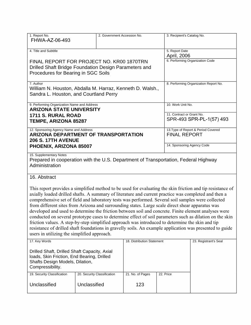
1. Report No. FHWA-AZ-06-493
2. Government Accession No.
3. Recipient's Catalog No.
4. Title and Subtitle
5. Report Date April, 2006
FINAL REPORT FOR PROJECT NO. KR00 1870TRN Drilled Shaft Bridge Foundation Design Parameters and Procedures for Bearing in SGC Soils
6. Performing Organization Code
7. Author William N. Houston, Abdalla M. Harraz, Kenneth D. Walsh., Sandra L. Houston, and Courtland Perry
8. Performing Organization Report No.
9. Performing Organization Name and Address ARIZONA STATE UNIVERSITY
10. Work Unit No.
1711 S. RURAL ROAD TEMPE, ARIZONA 85287
11. Contract or Grant No. SPR-493 SPR-PL-1(57) 493
12. Sponsoring Agency Name and Address ARIZONA DEPARTMENT OF TRANSPORTATION 206 S. 17TH AVENUE
13.Type of Report & Period Covered FINAL REPORT
PHOENIX, ARIZONA 85007 14. Sponsoring Agency Code
15. Supplementary Notes Prepared in cooperation with the U.S. Department of Transportation, Federal Highway Administration 16. Abstract This report provides a simplified method to be used for evaluating the skin friction and tip resistance of axially loaded drilled shafts. A summary of literature and current practice was completed and then a comprehensive set of field and laboratory tests was performed. Several soil samples were collected from different sites from Arizona and surrounding states. Large scale direct shear apparatus was developed and used to determine the friction between soil and concrete. Finite element analyses were conducted on several prototype cases to determine effect of soil parameters such as dilation on the skin friction values. A step-by-step simplified approach was introduced to determine the skin and tip resistance of drilled shaft foundations in gravelly soils. An example application was presented to guide users in utilizing the simplified approach. 17. Key Words Drilled Shaft, Drilled Shaft Capacity, Axial loads, Skin Friction, End Bearing, Drilled Shafts Design Models, Dilation, Compressibility.
18. Distribution Statement
23. Registrant's Seal
19. Security Classification Unclassified
20. Security Classification Unclassified
21. No. of Pages
123
22. Price

SI* (
MO
DER
N M
ETR
IC) C
ON
VER
SIO
N F
AC
TOR
S
APP
RO
XIM
ATE
CO
NVE
RSI
ON
S TO
SI U
NIT
S A
PPR
OXI
MA
TE C
ON
VER
SIO
NS
FRO
M S
I UN
ITS
Sym
bol
Whe
n Yo
u Kn
ow
Mul
tiply
By
To F
ind
Sym
bol
Sym
bol
Whe
n Yo
u Kn
ow
Mul
tiply
By
To F
ind
Sym
bol
LE
NG
TH
LEN
GTH
in
inch
es
25.4
m
illim
eter
s m
m
mm
m
illim
eter
s 0.
039
inch
es
in
ft fe
et
0.30
5 m
eter
s m
m
m
eter
s 3.
28
feet
ft
yd
yard
s 0.
914
met
ers
m
m
met
ers
1.09
ya
rds
yd
mi
mile
s 1.
61
kilo
met
ers
km
km
kilo
met
ers
0.62
1 m
iles
mi
A
REA
A
REA
in2
squa
re in
ches
64
5.2
squa
re m
illim
eter
s m
m2
mm
2 Sq
uare
milli
met
ers
0.00
16
squa
re in
ches
in
2
ft2 sq
uare
feet
0.
093
squa
re m
eter
s m
2 m
2 Sq
uare
met
ers
10.7
64
squa
re fe
et
ft2
yd2
squa
re y
ards
0.
836
squa
re m
eter
s m
2 m
2 Sq
uare
met
ers
1.19
5 sq
uare
yar
ds
yd2
ac
acre
s 0.
405
hect
ares
ha
ha
he
ctar
es
2.47
ac
res
ac
mi2
squa
re m
iles
2.59
sq
uare
kilo
met
ers
km2
km2
Squa
re k
ilom
eter
s 0.
386
squa
re m
iles
mi2
VO
LUM
E
VO
LUM
E
fl oz
flu
id o
unce
s 29
.57
milli
liter
s m
L m
L m
illilit
ers
0.03
4 flu
id o
unce
s fl
oz
gal
gallo
ns
3.78
5 lit
ers
L L
liter
s 0.
264
gallo
ns
gal
ft3 cu
bic
feet
0.
028
cubi
c m
eter
s m
3 m
3 C
ubic
met
ers
35.3
15
cubi
c fe
et
ft3
yd3
cubi
c ya
rds
0.76
5 cu
bic
met
ers
m3
m3
Cub
ic m
eter
s 1.
308
cubi
c ya
rds
yd3
NO
TE: V
olum
es g
reat
er th
an 1
000L
sha
ll be
sho
wn
in m
3 .
MA
SS
M
ASS
oz
ounc
es
28.3
5 gr
ams
g g
gram
s 0.
035
ounc
es
oz
lb
poun
ds
0.45
4 ki
logr
ams
kg
kg
kilo
gram
s 2.
205
poun
ds
lb
T sh
ort t
ons
(200
0lb)
0.
907
meg
agra
ms
(o
r “m
etric
ton”
) m
g (o
r “t”)
m
g m
egag
ram
s
(or “
met
ric to
n”)
1.10
2 sh
ort t
ons
(200
0lb)
T
TE
MPE
RA
TUR
E (e
xact
)
TE
MPE
RA
TUR
E (e
xact
)
º F Fa
hren
heit
tem
pera
ture
5(
F-32
)/9
or (F
-32)
/1.8
C
elsi
us te
mpe
ratu
re
º C
º C
Cel
sius
tem
pera
ture
1.
8C +
32
Fahr
enhe
it te
mpe
ratu
re
º F
IL
LUM
INA
TIO
N
ILLU
MIN
ATI
ON
fc
foot
can
dles
10
.76
lux
lx
lx
lux
0.09
29
foot
-can
dles
fc
fl
foot
-Lam
berts
3.
426
cand
ela/
m2
cd/m
2 cd
/m2
cand
ela/
m2
0.29
19
foot
-Lam
berts
fl
FO
RC
E A
ND
PR
ESSU
RE
OR
STR
ESS
FOR
CE
AN
D P
RES
SUR
E O
R S
TRES
S
lbf
poun
dfor
ce
4.45
ne
wto
ns
N
N
new
tons
0.
225
poun
dfor
ce
lbf
lbf/i
n2 po
undf
orce
per
sq
uare
inch
6.
89
kilo
pasc
als
kPa
kPa
kilo
pasc
als
0.14
5 po
undf
orce
per
sq
uare
inch
lb
f/in2
SI is
the
sym
bol f
or th
e In
tern
atio
nal S
yste
m o
f Uni
ts. A
ppro
pria
te ro
undi
ng s
houl
d be
mad
e to
com
ply
with
Sec
tion
4 of
AST
M E
380

TABLE OF CONTENTS INTRODUCTION............................................................................................................. 1
SUMMARY OF LITERATURE AND CURRENT PRACTICE................................. 3 SUMMARY OF HISTORIC USE............................................................................................ 3 ANALYTICAL APPROACHES.............................................................................................. 8
Introduction ................................................................................................................. 8 Tomlinson 2001 ........................................................................................................... 8 Meyerhoff 1976.......................................................................................................... 10 Reese and O'Neill 1989 (AASHTO METHOD) ......................................................... 10 Kulhawy 1989............................................................................................................ 10 Rollins, Clayton, Mikesell, and Blaise 1997.............................................................. 13
COMPARISON OF ACTUAL SKIN FRICTION FACTORS TO PREDICTED FOR DRILLED SHAFT IN GRANULAR SOIL ........................................................ 15
INTRODUCTION............................................................................................................... 15 LOAD TESTS................................................................................................................... 15 VALUES OF FS DERIVED FROM DIRECT FIELD MEASUREMENTS ..................................... 16 PREDICTED VALUES OF FS .............................................................................................. 16 RESULTS......................................................................................................................... 17 DILATION ....................................................................................................................... 30
REPORT ON PRELIMINARY FINITE ELEMENT ANALYSES OF TWO CASE HISTORY STUDIES OF AXIALLY LOADED DRILLED SHAFTS ...................... 33
INTRODUCTION............................................................................................................... 33 CHARACTERISTICS OF THE SGC SOILS ........................................................................... 33 AXIAL COMPRESSION LOADING ON DRILLED SHAFTS.................................................... 33
Soil Profile................................................................................................................. 34 Pile Configuration ..................................................................................................... 34 Finite Element Analysis ............................................................................................. 34 Effect of Dilation Angle.............................................................................................. 37 Best Fit Indicator....................................................................................................... 38 Selection of Best Set of Parameters for SGC............................................................. 39
UPLIFT LOADING ON DRILLED SHAFT TEST ................................................................... 39 Soil Profile................................................................................................................. 39 Pile Configuration ..................................................................................................... 40 Finite Element Analysis ............................................................................................. 40
CONCLUSIONS FROM STUDY OF LITERATURE AND CURRENT PRACTICE......................... 43
DEVELOPMENT OF WORK PLAN FOR COMPLETION OF THE PROJECT AND ASSESSMENT OF PROGNOSIS FOR SUCCESS........................................... 45
DATA GAPS .................................................................................................................... 45 WORK PLAN OVERVIEW................................................................................................. 46 PROGNOSIS FOR SUCCESS .............................................................................................. 48

FIELD TESTING.........................................................................................................................53 IN-SITU DENSITY.........................................................................................................................53
LAB TESTING ............................................................................................................................59 GRAIN SIZE DISTRIBUTION..........................................................................................................59
LARGE SCALE SHEAR TESTING ...................................................................................................68 Testing Procedure ..................................................................................................................69 Direct Shear Lab Test Program .............................................................................................74 Test Results.............................................................................................................................75
MODELING OF THE DATA ...........................................................................................................85
K VALUES FROM THE DIRECT SHEAR TEST ................................................................................87
NUMERICAL ANALYSES ........................................................................................................89 FINITE ELEMENT MODEL.............................................................................................................89
Analysis...................................................................................................................................90 POINT OF THE MOUNTAIN EAST SITE .........................................................................................92
K-DEPTH-% GRAVEL MODEL .....................................................................................................95
RECOMMENDED DESIGN PROCEDURES FOR DRILLED SHAFTS IN GRAVELLY MATERIALS ......................................................................................99
COMPARISON OF THE ULTIMATE TIP RESISTANCE BY EQUATION 7 USING BEREZANTSEV BEARING CAPACITY FACTORS WITH THE MEASURED TIP RESISTANCE FOR THE BECKWITH AND BEDENKOP TEST ON SALT RIVER SGC...........................................................102
EXAMPLE DRILLED SHAFT DESIGN, USING THE RECOMMENDED PROCEDURE.....................................................................105
CONCLUSIONS ........................................................................................................................109
REFERENCES...........................................................................................................................111

LIST OF FIGURES
FIGURE 1: RELATIONSHIP BETWEEN SPT N-VALUES AND ANGLE OF SHEARING RESISTANCE [TOMLINSON, 2001] .......................................................... 9
FIGURE 2: END-BEARING CAPACITY FACTORS [HANSEN, 1961;BEREZANTSEV,1961] .................... 9 FIGURE 3. PREDICTED VS. ACTUAL FS VALUES, ALL METHODS..................................................... 17 FIGURE 4. PREDICTED VS. ACTUAL FS VALUES, TOMLINSON AND KULHAWY ............................... 18 FIGURE 5. PREDICTED VS. ACTUAL FS VALUES, MEYERHOFF ........................................................ 18 FIGURE 6. PREDICTED VS. ACTUAL FS VALUES, REESE & O’NEILL ............................................... 19 FIGURE 7. PREDICTED VS. ACTUAL FS VALUES, ROLLINS ET AL. ................................................... 19 FIGURE 8. P VS. A VALUES, TOMLINSON AND KULHAWY, BY SOIL TYPE...................................... 20 FIGURE 9. P VS. A VALUES, MEYERHOFF, BY SOIL TYPE .............................................................. 20 FIGURE 10. P VS. A VALUES, REESE AND O’NEILL, BY SOIL TYPE ............................................... 21 FIGURE 11. P VS. A VALUES, ROLLINS ET AL., BY SOIL TYPE........................................................ 21 FIGURE 12. P VS. A VALUES, TOMLINSON AND KULHAWY, BY TEST TYPE ................................... 22 FIGURE 13. P VS. A VALUES, MEYERHOFF, BY TEST TYPE............................................................ 22 FIGURE 14. P VS. A VALUES, REESE AND O’NEILL, BY TEST TYPE............................................... 23 FIGURE 15. P VS. A VALUES, ROLLINS ET AL., BY TEST TYPE....................................................... 30 FIGURE 16. AVERAGE P/A VS. % GRAVEL, ALL METHODS EXCEPT ROLLINS ET AL...................... 24 FIGURE 17. AVERAGE P/A VS. % GRAVEL, ROLLINS ET AL........................................................... 25 FIGURE 18. AVERAGE P/A VS. DEPTH TO MID-LAYER, ALL METHODS EXCEPT ROLLINS ET AL. .. 26 FIGURE 19. AVERAGE P/A VS. DEPTH TO MID-LAYER, ROLLINS ET AL......................................... 26 FIGURE 20. AVERAGE P/A VS. TEST TYPE, ALL METHODS EXCEPT ROLLINS ET AL. ..................... 27 FIGURE 21. AVERAGE P/A VS. TEST TYPE, ROLLINS ET AL. .......................................................... 27 FIGURE 22. K VS. % GRAVEL ........................................................................................................ 28 FIGURE 23. KPS VS. % GRAVEL ...................................................................................................... 29 FIGURE 24. K VS. DEPTH TO MID-LAYER...................................................................................... 29 FIGURE 25. K PS VS. DEPTH TO MID-LAYER ................................................................................. 30 FIGURE 26: TYPICAL GRAIN SIZE DISTRIBUTION OF SGC SOIL..................................................... 32 FIGURE 27: PILE CONFIGURATION ................................................................................................. 34 FIGURE 28: DRUCKER-PRAGER MODEL. ........................................................................................ 35 FIGURE 29: FIELD LOAD-DEFLECTION CURVE............................................................................... 35 FIGURE 30: EFFECT OF SOIL MODULUS, E, ON THE LOAD DEFLECTION CURVE. ............................. 36 FIGURE 31: EFFECT OF SOIL ANGLE OF INTERNAL FRICTION, Ø,
ON THE LOAD DEFLECTION CURVE............................................................................ 36 FIGURE 32: EFFECT OF SOIL DILATION ANGLE ON RESULTS.......................................................... 37 FIGURE 33: SET OF TRIALS OF MATCH FIELD LOAD-DEFLECTION CURVE. .................................... 37 FIGURE 34: R2 VALUES FOR DIFFERENT SETS OF Ø AND Ψ............................................................. 38 FIGURE 35: CURVE OF MAXIMUM R2 VALUES, FOR ψ VS φ. .......................................................... 38 FIGURE 36: GRAIN SIZE DISTRIBUTION FOR THE SOIL AT UTAH SITE.............................................. 39 FIGURE 37: PILE CONFIGURATION ................................................................................................. 40 FIGURE 38: LOAD DEFLECTION CURVE FOR THE UPLIFT TEST....................................................... 41 FIGURE 39: EFFECT OF SOIL MODULUS, E ON LOAD DEFLECTION CURVE. .................................... 41 FIGURE 40: EFFECT OF COEFFICIENT OF FRICTION BETWEEN PILE AND SOIL, F. ............................ 42 FIGURE 41: EFFECT OF COEFFICIENT OF FRICTION, F, ON LOAD DEFLECTION CURVE.................... 42 FIGURE 42: BEST FIT FOR THE UPLIFT LOAD TEST......................................................................... 43

FIGURE 43: K VS DEPTH FOR DIFFERENT GRAVEL CONTENT ......................................................... 49 FIGURE 44: GRAVEL CONTENT VS. UNIT WEIGHT, �-APPROXIMATE RELATIONSHIP .................... 49 FIGURE 45: GRAVEL CONTENT VS. φ` VALUE-APPROXIMATE RELATIONSHIP................................ 50 FIGURE 46: MEASURED VS. PREDICTED FOR A NEW EMPIRICAL MODEL ....................................... 51 FIGURE 47: HOLE IS EXCAVATED USING THE BACKHOE. ............................................................... 54 FIGURE 48: THE MATERIAL IS DUMPED (COLLECTED) IN A LOADER TO BE WEIGHED.................... 54 FIGURE 49: THE HOLE IS LINED WITH A PLASTIC SHEET................................................................. 55 FIGURE 50: THE WATER TANK USED TO FILL THE HOLE. .............................................................. 55 FIGURE 51: HOLE FILLED WITH WATER......................................................................................... 56 FIGURE 52: COLLECTED SAMPLES ................................................................................................. 56 FIGURE 53: GRAIN SIZE DISTRIBUTION FOR MATERIAL # 1, 91ST AVENUE (AZ1)......................... 60 FIGURE 54: GRAIN SIZE DISTRIBUTION FOR MATERIAL # 2, 91ST AVENUE (AZ2)......................... 60 FIGURE 55: GRAIN SIZE DISTRIBUTION FOR MATERIAL # 3, 91ST AVENUE (AZ3)......................... 60 FIGURE 56: GRAIN SIZE DISTRIBUTION FOR MATERIAL # 4, 51ST AVENUE (AZ1)......................... 61 FIGURE 57: GRAIN SIZE DISTRIBUTION FOR MATERIAL # 5, 51ST AVENUE (AZ2)......................... 61 FIGURE 58: GRAIN SIZE DISTRIBUTION FOR MATERIAL # 6, 51ST AVENUE (AZ3)......................... 61 FIGURE 59: GRAIN SIZE DISTRIBUTION FOR MATERIAL # 7, MAPLETON (UT1)............................. 62 FIGURE 60: GRAIN SIZE DISTRIBUTION FOR MATERIAL # 8, MAPLETON (UT2)............................. 62 FIGURE 61: GRAIN SIZE DISTRIBUTION FOR MATERIAL # 9,
POINT OF THE MOUNTAIN EAST (UT1). ..................................................................... 62 FIGURE 62: GRAIN SIZE DISTRIBUTION FOR MATERIAL # 10,
POINT OF THE MOUNTAIN EAST (UT2). ..................................................................... 63 FIGURE 63: GRAIN SIZE DISTRIBUTION FOR MATERIAL # 11,
POINT OF THE MOUNTAIN WEST (UT1). .................................................................... 63 FIGURE 64: GRAIN SIZE DISTRIBUTION FOR MATERIAL # 12,
POINT OF THE MOUNTAIN WEST (UT2). .................................................................... 63 FIGURE 65: GRAIN SIZE DISTRIBUTION FOR MATERIAL # 13, GARCIA RIVER (CA1). .................... 64 FIGURE 66: GRAIN SIZE DISTRIBUTION FOR MATERIAL # 14, GUALALA RIVER (CA2).................. 64 FIGURE 67: GRAIN SIZE DISTRIBUTION FOR MATERIAL # 15, REDWOOD CREEK (CA3). ............... 64 FIGURE 68: GRAIN SIZE DISTRIBUTION FOR MATERIAL # 16, NAVARRO RIVER (CA4). ................ 65 FIGURE 69: GRAIN SIZE DISTRIBUTION FOR MATERIAL # 17, COLUMBIA RIVER (OR1). ............... 65 FIGURE 70: GRAIN SIZE DISTRIBUTION FOR MATERIAL # 18, ROGUE RIVER (OR2). ..................... 66 FIGURE 71: GRAIN SIZE DISTRIBUTION FOR ALL MATERIALS........................................................ 66
FIGURE 72: MEASURED d
w
γγ
VALUES VERSUS PREDICTED ............................................................ 68
FIGURE 73: LARGE SCALE SHEAR BOX.......................................................................................... 69 FIGURE 74: MATERIAL IS MIXED DRY FIRST AND THEN WETTED. ................................................... 71 FIGURE 75: COMPACTING MATERIAL IN LAYERS........................................................................... 71 FIGURE 76: A COVER PLATE USED TO MAKE SURE MATERIAL IS FLUSH TO BOX TOP.................. 72 FIGURE 77: MATERIAL IS REMOVED FROM THE UPPER HALF OF THE BOX. ...................................... 72 FIGURE 78: POURING CONCRETE INTO THE BOX............................................................................. 73 FIGURE 79: LOAD DEFLECTION CURVE FOR MATERIAL #1. ........................................................... 75 FIGURE 80: LOAD DEFLECTION CURVE FOR MATERIAL #3. ........................................................... 76 FIGURE 81: LOAD DEFLECTION CURVE FOR MATERIAL #7. ........................................................... 76 FIGURE 82: LOAD DEFLECTION CURVE FOR MATERIAL #9. ........................................................... 77 FIGURE 83: LOAD DEFLECTION CURVE FOR MATERIAL #16. ......................................................... 77

FIGURE 84: LOAD DEFLECTION CURVE FOR MATERIAL #17. ......................................................... 78 FIGURE 85: SHEAR STRENGTH ENVELOPE FOR MATERIAL #1. ....................................................... 78 FIGURE 86: SHEAR STRENGTH ENVELOPE FOR MATERIAL #3. ....................................................... 79 FIGURE 87: SHEAR STRENGTH ENVELOPE FOR MATERIAL #7. ....................................................... 79 FIGURE 88: SHEAR STRENGTH ENVELOPE FOR MATERIAL #9. ....................................................... 80 FIGURE 89: SHEAR STRENGTH ENVELOPE FOR MATERIAL #16. ..................................................... 80 FIGURE 90: SHEAR STRENGTH ENVELOPE FOR MATERIAL #17. ..................................................... 81 FIGURE 91: SUMMARY OF THE SHEAR STRENGTH ENVELOPES FOR ALL CHOSEN MATERIALS. ...... 81 FIGURE 92: HORIZONTAL DEFORMATION VERSUS VERTICAL DEFORMATION FOR MATERIAL #1. . 82 FIGURE 93: HORIZONTAL DEFORMATION VERSUS VERTICAL DEFORMATION FOR MATERIAL #3. . 82 FIGURE 94: HORIZONTAL DEFORMATION VERSUS VERTICAL DEFORMATION FOR MATERIAL #7. . 83 FIGURE 95: HORIZONTAL DEFORMATION VERSUS VERTICAL DEFORMATION FOR MATERIAL #9. . 83 FIGURE 96: HORIZONTAL DEFORMATION VERSUS VERTICAL DEFORMATION FOR MATERIAL #16. 84 FIGURE 97: HORIZONTAL DEFORMATION VERSUS VERTICAL DEFORMATION FOR MATERIAL #17. 84 FIGURE 98: MEASURED Ψ VALUES VERSUS PREDICTED................................................................ 86 FIGURE 99: MEASURED VERSUS PREDICTED δ VALUES. ................................................................ 86 FIGURE 100: HALF SYMMETRY OF SHAFT AND SOIL DISCRETIZATION MESH................................88
FIGURE 101: P-Δ CURVES WITH DIFFERENT FINITE ELEMENT TRIALS FOR 15 FT SHAFT AT MAPLETON....................................................................................... 91
FIGURE 102: P-Δ CURVES WITH DIFFERENT FINITE ELEMENT TRIALS FOR 10 FT SHAFT AT MAPLETON....................................................................................... 91
FIGURE 103:P-Δ CURVES WITH DIFFERENT FINITE ELEMENT TRIALS FOR 5 FT SHAFT AT MAPLETON ......................................................................................... 92
FIGURE 104:P-Δ CURVES WITH DIFFERENT FINITE ELEMENT TRIALS FOR 5 FT SHAFT AT PT. EAST ............................................................................................................... 94
FIGURE 105: P-Δ CURVES WITH DIFFERENT FINITE ELEMENT TRIALS FOR 10 FT SHAFT AT PT. EAST .................................................................................................................... 94
FIGURE 106: P-Δ CURVES WITH DIFFERENT FINITE ELEMENT TRIALS FOR 15 FT SHAFT AT PT. EAST ............................................................................................................... 95
FIGURE 107: P-Δ CURVES WITH DIFFERENT FINITE ELEMENT TRIALS FOR 20 FT SHAFT AT PT. EAST ............................................................................................................... 95
FIGURE 108: K-VALUE VERSUS DEPTH (FROM FINAL ELEMENT AND DIRECT SHEAR).................. 96 FIGURE 109: COMPARISON BETWEEN DIFFERENT METHODS USED TO REPRESENT
K-VERSUS-%GRAVEL ................................................................................................ 97

LIST OF TABLES
TABLE 1: LEGEND FOR PLAN DESCRIPTION AND SUMMARY............................................................ 4 TABLE 2: ζ TERMS ....................................................................................................................... 11 TABLE 3: TYPICAL ED VALUES ...................................................................................................... 12 TABLE 4: β VALUES...................................................................................................................... 13 TABLE 5: LOAD TESTS .................................................................................................................. 15 TABLE 6: RIVER BEDS AND GRAVEL PIT SITES .............................................................................. 53 TABLE 7: MOIST IN-SITU DENSITY ................................................................................................ 57 TABLE 8: NATURAL WATER CONTENT .......................................................................................... 59 TABLE 9: VARIOUS PARAMETERS OF THE GRAIN SIZE DISTRIBUTION FOR ALL MATERIALS.......... 67 TABLE 10: PROPERTIES OF THE CHOSEN SIX MATERIALS TO BE TESTED
IN LARGE SCALE SHEAR BOX .................................................................................... 74 TABLE 11: LARGE SCALE SHEAR BOX TEST MATRIX .................................................................... 74 TABLE 12: SUMMARY OF THE LARGE SCALE SHEAR BOX TEST RESULTS...................................... 85 TABLE 13: FINITE ELEMENT TRIALS FOR 15FT SHAFT AT MAPLETON............................................ 90 TABLE 14: FINITE ELEMENT TRIALS FOR 10FT SHAFT AT MAPLETON............................................ 90 TABLE 15: FINITE ELEMENT TRIALS FOR 5FT SHAFT AT MAPLETON.............................................. 90 TABLE 16: FINITE ELEMENT TRIALS FOR 5FT SHAFT AT POINT OF THE MOUNTAIN EAST .............. 92 TABLE 17: FINITE ELEMENT TRIALS FOR 10FT SHAFT AT POINT OF THE MOUNTAIN EAST ............ 93 TABLE 18: FINITE ELEMENT TRIALS FOR 15FT SHAFT AT POINT OF THE MOUNTAIN EAST ............ 93 TABLE 19: FINITE ELEMENT TRIALS FOR 20FT SHAFT AT POINT OF THE MOUNTAIN EAST ............ 93 TABLE 20: FACTOR OF SAFETY VS. DEFLECTION FOR DRILLED SHAFT SKIN FRICTION................ 100 TABLE 21: FACTOR OF SAFETY VS. DEFLECTION FOR DRILLED SHAFT TIP RESISTANCE.............. 100 TABLE 22: RESULTS FROM STEPS 1 AND 2 – EXAMPLE DESIGN ................................................... 105 TABLE 23: RESULTS FROM STEPS 3, 4, AND 5 – EXAMPLE DESIGN............................................... 105 TABLE 24: RESULTS FROM STEPS 6, 7, AND 8 – EXAMPLE DESIGN............................................... 106 TABLE 25: COMPARISON OF QTOTAL (DESIGN) AND Q APPLIED BY THE SUPERSTRUCTURE
AND INDICATED ACTIONS ........................................................................................ 107

ACKNOWLEDGMENTS
The authors wish to thank Christ Dimitroplos and all ADOT personnel and consultants associated with this project for their support, patience, and perseverance in seeing this project through. Financial support for the completion of this project was requested and received from the Federal Highway Administration and this support is also gratefully acknowledged. We would also like to thank Kyle Rollins for his encouragement and assistance in gaining access to certain sites for testing and sampling and his discussions with us on the research project.


1
INTRODUCTION
Drilled shafts are used extensively by the Arizona Department of Transportation (ADOT) for foundation support of transportation structures. Drilled shafts have become the preferred deep foundation element in the state because soil conditions are usually unfavorable to driven piles, scour depths on the ephemeral river channels are quite large, and there is increased confidence in the bearing layer afforded by the drilled shaft construction process. These foundations are typically designed using American Association of State Highway and Transportation Officials (AASHTO) guidelines and local experience. Coarse granular materials are commonly found in the high energy riverine environments of the Arizona deserts. Variously described as river-run, sand-gravel-cobbles, or SGC, these materials are encountered frequently at bridge foundation elements because of their proximity to the water courses. Typically dense and containing particles as large as boulder-sized materials, SGC is usually sub-rounded due to transport and the larger particles are very hard. The material is frequently clean and uncemented in the upper portions of the deposit but contains low- to moderate-plasticity fines and/or light cementation which generates some apparent cohesion below a depth of 20 to 30 feet. Extremely difficult to characterize, the material is impossible to sample and test. Lack of cohesion makes the sampling process difficult for any soil but the large particle sizes of SGC compound the problem dramatically. Particle sizes in excess of 12 inches or more may be found, requiring samples with a minimum diameter of 40 inches. Even if samples could be obtained, conventional lab equipment is not designed to handle the large size. Two approaches are generally adopted in geotechnical practice when sampling and testing of the material is not possible: 1) field testing and 2) extrapolation of test data and relationships for finer grained cohesionless material. Field tests involve an extremely large volume of soil and are best conducted on a drilled shaft of a size used in practice. Due to the very large capacities developed in SGC soils, testing of this kind is difficult and expensive to perform. ADOT has conducted some field testing on deep foundations with the most relevant in SGC soils — that reported by Beckwith and Bedenkop (1973)—providing information only on tip resistance. Extrapolation of test data and relationships for finer grained cohesionless material is the method used somewhat exclusively in the past design practice in Arizona. Extrapolation is not trivial and requires an excellent model that takes into account a variety of parameters. Most of the models employed in the past have not properly accounted for the differences in grain size and density between finer grained soils and SGC, especially as it relates to dilatancy. The most common approach has been a direct utilization of the results for finer grained materials (such as those outlined in the AASHTO standard as discussed by Reese and O’Neill 1989) without any accounting at all for changes in grain size and density. This approach is very conservative, as will be demonstrated subsequently. To examine these issues an ADOT research project was initiated in 2000 (SPR-493, Bridge Foundation Design Parameters and Procedures for Bearing in SGC Soil). This project's purpose was to consider possible modifications to the existing procedures for use in gravelly materials. The modifications would likely take the form of a set of recommendations for gravelly soils such

2
as SGC soils. New design procedures would need to be appropriate for a wide range of gradations of gravelly materials. A potentially measurable property of the soil in place (such as gradation) was to be related to the recommended values. Following an exhaustive literature study, a mechanistic model was to be developed and calibrated that predicts axial behavior. Full-scale load tests already reported in the literature that are representative of the soil conditions, loading geometry, and boundary conditions which ADOT typically encounters were to be used to calibrate the model. This report presents the results of all efforts to date on SPR-493. It includes a summary of literature and current practice, a summary of historic use, analytical approaches currently used, data gaps, and reports on finite element analyses performed, field and lab testing results, development of models and design methodology, and presentation of an example design of a drilled shaft in gravelly material.

3
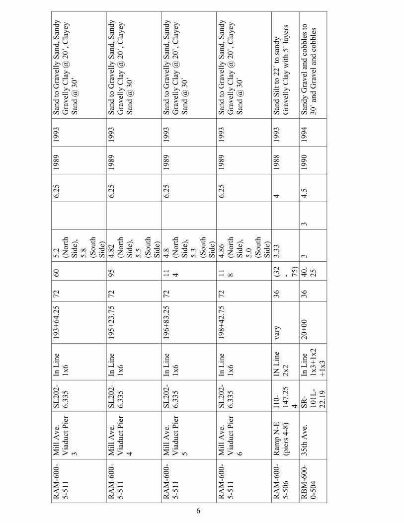
SUMMARY OF LITERATURE AND CURRENT PRACTICE An exhaustive search of the literature found nineteen articles, three Federal Highway Admin-istration (FHWA) reports, and one report prepared for ADOT that involved load tests on drilled shafts in coarse granular material. At a majority of the sites reported in these studies only strata of gravelly material were encountered. Typically, the shafts were instrumented and load transfer curves given. From these load transfer curves the average unit side resistance on the shaft over the depth of the gravelly strata could be calculated. The amount of information given on the strata was generally limited to Standard Penetration Test (SPT) N-values, Unified Soil Classification System (USCS) classifications, and general boring log descriptions. Additional information including results of Cone Penetration Tests (CPT), Pressure-Meter Tests (PMT) and grain-size distributions (GSD) were given only in a small number of cases. Ideally, densities and strength parameters also would have been provided, but these data were rare. Summary of Historic Use The purpose of this section is to display how drilled shafts are used in axial load applications in Arizona, specifically with regards to shaft geometry, group geometry, and soil conditions. Table 1 following includes first a legend for use with the inventory list provided as the continuation of Table 1.
4
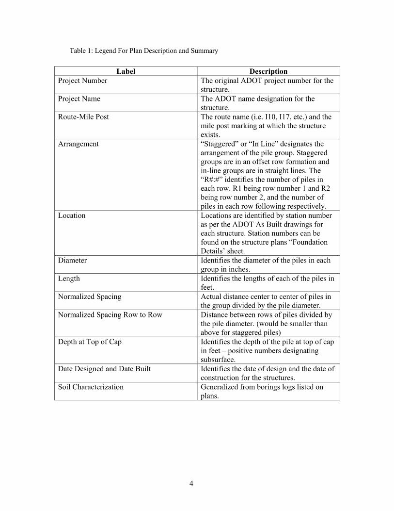
Table 1: Legend For Plan Description and Summary
Label Description Project Number The original ADOT project number for the
structure. Project Name The ADOT name designation for the
structure. Route-Mile Post The route name (i.e. I10, I17, etc.) and the
mile post marking at which the structure exists.
Arrangement “Staggered” or “In Line” designates the arrangement of the pile group. Staggered groups are in an offset row formation and in-line groups are in straight lines. The “R#:#” identifies the number of piles in each row. R1 being row number 1 and R2 being row number 2, and the number of piles in each row following respectively.
Location Locations are identified by station number as per the ADOT As Built drawings for each structure. Station numbers can be found on the structure plans “Foundation Details’ sheet.
Diameter Identifies the diameter of the piles in each group in inches.
Length Identifies the lengths of each of the piles in feet.
Normalized Spacing Actual distance center to center of piles in the group divided by the pile diameter.
Normalized Spacing Row to Row Distance between rows of piles divided by the pile diameter. (would be smaller than above for staggered piles)
Depth at Top of Cap Identifies the depth of the pile at top of cap in feet – positive numbers designating subsurface.
Date Designed and Date Built Identifies the date of design and the date of construction for the structures.
Soil Characterization Generalized from borings logs listed on plans.

5
Proj
. Num
. Pr
oj. N
ame
Rte
M
ile
Post
Arr
. Lo
c.
Dia
.Lt
h N
orm
Sp
cg
Nor
m
Spcg
R
ow
to
Row
Dep
th
at T
op
of
Cap
Dat
e D
es.
Dat
e B
uilt
Soil
Cha
r.
RA
M-6
00-
3-51
4 W
ashi
ngto
n St
. Pie
r-1
SR14
3-2.
07
InLi
ne1x
4 13
0+08
60
39
4.
7
5 19
89
1993
Si
lty sa
nd to
San
d &
Gra
vel
with
cem
ent t
o sa
nd &
Gra
vel
Con
glom
erat
e@30
ft R
AM
-600
-3-
514
Was
hing
ton
St. P
ier-
2 SR
143-
2.07
In
Line
1x4
130+
98
60
22
4.7
5
1989
19
93
Silty
sand
to S
and
& G
rave
l w
ith c
emen
t to
sand
& G
rave
l C
ongl
omer
ate@
30ft
RA
M-6
00-
3-51
4 W
ashi
ngto
n St
. Pie
r-3
SR14
3-2.
07
InLi
ne1x
4 13
1+77
60
22
4.
7
5 19
89
1993
Si
lty sa
nd to
San
d &
Gra
vel
with
cem
ent t
o sa
nd &
Gra
vel
Con
glom
erat
e@30
ft R
AM
-600
-3-
514
Was
hing
ton
St. P
ier-
4 SR
143-
2.07
In
Line
1x4
132+
50.5
60
33
4.
7
5 19
89
1993
Si
lty sa
nd to
San
d &
Gra
vel
with
cem
ent t
o sa
nd &
Gra
vel
Con
glom
erat
e@30
ft R
AM
-600
-3-
514
Was
hing
ton
St. P
ier-
5 SR
143-
2.07
In
Line
1x4
133+
23
60
21
4.7
5
1989
19
93
Silty
San
d to
20’
Gra
vel &
sa
nd &
Wea
ther
ed G
rani
te
RA
M-6
00-
5-51
1 M
ill A
ve.
Via
duct
Pie
r 1
SL20
2-6.
335
In L
ine
1x6
190+
81.2
572
84
4.
6 (N
orth
Si
de),
6.25
(S
outh
Si
de)
6.
25
1989
19
93
Sand
to G
rave
lly S
and,
San
dy
rave
lly C
lay
@ 2
0’, C
laye
y Sa
nd 3
0’
RA
M-6
00-
5-51
1
Mill
Ave
. V
iadu
ct P
ier
2
SL20
2-6.
335
In
Lin
e 1x
6
192+
22.7
5 72
61
6.
1
6.
25
1989
19
93
Sand
to G
rave
lly S
and,
San
dy
Gra
velly
Cla
y @
20’
, Cla
yey
Sand
@ 3
0’
6
RA
M-6
00-
5-51
1
Mill
Ave
. V
iadu
ct P
ier
3
SL20
2-6.
335
In
Lin
e 1x
6
193+
64.2
5 72
60
5.
2 (N
orth
Si
de),
5.8
(Sou
th
Side
)
6.
25
1989
19
93
Sand
to G
rave
lly S
and,
San
dy
Gra
velly
Cla
y @
20’
, Cla
yey
Sand
@ 3
0’
RA
M-6
00-
5-51
1
Mill
Ave
. V
iadu
ct P
ier
4
SL20
2-6.
335
In
Lin
e 1x
6
195+
23.7
5 72
95
4.
82
(Nor
th
Side
), 5.
5 (S
outh
Si
de)
6.
25
1989
19
93
Sand
to G
rave
lly S
and,
San
dy
Gra
velly
Cla
y @
20’
, Cla
yey
Sand
@ 3
0’
RA
M-6
00-
5-51
1
Mill
Ave
. V
iadu
ct P
ier
5
SL20
2-6.
335
In
Lin
e 1x
6
196+
83.2
5 72
11 4
4.
8 (N
orth
Si
de),
5.3
(Sou
th
Side
)
6.
25
1989
19
93
Sand
to G
rave
lly S
and,
San
dy
Gra
velly
Cla
y @
20`
, Cla
yey
Sand
@ 3
0`
RA
M-6
00-
5-51
1
Mill
Ave
. V
iadu
ct P
ier
6
SL20
2-6.
335
In
Lin
e 1x
6
198+
42.7
5 72
11 8
4.
86
(Nor
th
Side
), 5.
0 (S
outh
Si
de)
6.
25
1989
19
93
Sand
to G
rave
lly S
and,
San
dy
Gra
velly
Cla
y @
20`
, Cla
yey
Sand
@ 3
0`
RA
M-6
00-
5-50
6
Ram
p N
-E
(pie
rs 4
-8)
I10-
147.
254
IN L
ine
2x2
va
ry
36
(32
- 75)
3.33
4
1988
19
93
Sand
Silt
to 2
2` to
sand
y G
rave
lly C
lay
with
5` l
ayer
s
RB
M-6
00-
0-50
4
35th
Ave
. SR
-10
1L-
22.1
9
In L
ine
1x3+
1x2
+1x3
20+0
0
36
40.
25
3
3
4.5
19
90
1994
Sa
ndy
Gra
vel a
nd c
obbl
es to
30
` and
Gra
vel a
nd c
obbl
es

7
RB
M-6
00-
0-50
2
Skun
k C
reek
B
ridge
, Pi
ers 1
, 2, 3
SR41
7-21
3.49
In
Lin
e 1x
5
746+
19.0
, 74
7+40
.0,
748+
61.0
60
73
4.5
5
1986
19
90
RA
M-6
00-
0523
R
amp
S-E,
Pi
er 1
SL
101-
2
In L
ine
1x3+
1x2
+1x3
36
30
3
3
1989
RA
M-6
00-
0523
R
amp
S-E,
Pi
er 2
SL
101-
2
In L
ine
1x3+
1x2
+1x3
36
62
3
3
1989
RA
M-6
00-
0523
R
amp
S-E,
Pi
er 3
,4,5
SL
101-
2
In L
ine
3x4
36
62
3
3
19
89
RA
M-6
00-
0523
R
amp
W-N
, Pi
er 1
SL
101-
2
In L
ine
2x3
27
+88.
52
36
3
3
5
19
90
RA
M-6
00-
0523
R
amp
W-N
, Pi
er 2
SL
101-
2
In L
ine
2x5
33
+76.
52
36
3
3
5
19
90

8
Analytical Approaches Introduction All methods for determining the axial capacity of drilled shafts are based upon the general equation:
ult p sQ Q Q W= + − (1)
where Qult is the ultimate axial capacity of the shaft, Qp is the bearing capacity component of the shaft and is contributed by the tip, Qs is the side resistance component of the shaft and is contributed by side friction, and W is the weight of the shaft. It is generally agreed that the weight of the shaft is approximately equal to the weight of the soil displaced during drilling. Therefore, the W term is often neglected leaving: ult p sQ Q Q= + (2)
The components Qp and Qs are calculated by the following two equations:
p p pQ q A= (3)
s s sQ f A= (4)
where qp is the base resistance per unit area, Ap is the cross-sectional area of the tip, fs is the shaft resistance per unit area, and As is the surface area of the sides of the shaft in contact with the soil. For differing layers of soils, Qs consists of contributions from each layer. The methods that follow are focused on determining qp and fs for cohesionless granular soils. The methods are presented in their most updated form.
Tomlinson 2001 The unit skin resistance is calculated by Tomlinson (2001): tansf Kσ δ′= ≤ 110 [kN/m2] (5)
where σ ′ equals the average effective overburden pressure over the depth of a soil layer, K is a coefficient of horizontal soil stress, and δ is the soil-pile friction interface angle obtained from laboratory shear box tests. For drilled shafts in coarse soils, K equals 0.7 to 1.0 times K0 with the higher value corresponding to good construction technique. The coefficient of earth pressure at rest, K0, is the ratio between the horizontal and the vertical effective stresses, and is found from the following equation:
0 (1 sin )K OCRφ′= − (6)
where φ′ is the effective angle of shearing resistance in a soil and OCR is the over-consolidation ratio. The over-consolidation ratio is the ratio of the maximum previous vertical effective overburden pressure to the existing vertical effective overburden pressure. The value of φ′ is usually considered to be the same as the φ found using Standard Penetration Tests (SPT) N-values. The relationship between SPT and φ as established by Peck et al. (1967, p.310) and provided by Tomlinson is shown in Figure 1.

9
Figure 1: Relationship Between SPT N-Values and Angle of Shearing Resistance
[Tomlinson 2001] Tomlinson recommends that the φ value be assumed representative of loose conditions when considering drilled shafts. However, when the shafts are drilled and constructed using bentonite slurry, the φ value should correspond to undisturbed conditions. The unit base resistance is calculated by: p qq Nσ ′= (7)
where qN is a bearing capacity factor and is found using a chart that includes recommendations from both Hansen (1961) and Berezantsev (1961) (Figure 2). The φ value is also found from SPT tests and should correspond to loose conditions for dry constructed drilled shafts and undisturbed conditions for shafts constructed under bentonite slurry.
Figure 2: End-Bearing Capacity Factors (Hansen 1961; Berezantsev 1961)
10
Meyerhoff 1976 Meyerhoff gives the unit side resistance as:
100sNf = tons per square foot ( tsf) (8)
where N is the average SPT N-value, not corrected for overburden pressure.
The unit base resistance can be calculated as: 1.2p corrq N= tsf (9) where Ncorr is the SPT N-value corrected for effective overburden pressure. The value of Ncorr is referenced from Peck et al. (1967: 310) and standardizes N-values to the N-value at an effective overburden pressure of 1 tsf (Reese and O'Neill 1989). It is found by multiplying the field N-value by a correction factor CN:
10200.77logNCσ
=′ (10)
where ′σ is the vertical effective stress in tsf. Reese and O'Neill 1989 (AASHTO METHOD) The unit side resistance for a given layer is given by Reese and O’Neill and adopted by AASHTO as: sf βσ ′= (11) where β is equivalent to tanK δ in equation (5) and is given by the function 0.51.5 0.135 ;zβ = − 0.25 1.20β≤ ≤ , (12) σ ′ is the vertical effective stress at the middle of a layer, and z is the depth to the middle of a layer in feet (Reese and O’Neill 1989; AASHTO 1998). The unit base resistance is given by the following formula: 0.60pq N= tsf 45≤ tsf (13) where N is the uncorrected N-value from the SPT test within a distance of 2Bb below the tip of the shaft. Bb is the diameter of the base of the shaft. Kulhawy 1989 The unit side resistance is found using the general equation: tansf Kσ δ′= (14) where δ can be expressed as a function of φ′ . The ratio /δ φ′ is a function of construction technique and for good construction techniques equals 1. For poor slurry construction techniques where sufficient care was not taken to ensure that all of the slurry was expelled from the hole or the slurry was mixed together with and infiltrated the sides of the hole, /δ φ′ is reduced to 0.8 or lower (Kulhawy 1989). As with Tomlinson, K is a function of K0, the original in-situ coefficient of horizontal earth pressure. Kulhawy recommends that K0 can be found from the following:

11
( ) ( )0 1 sinmaxmax
31 sin 14
OCR OCRKOCROCR φ
φ ′−
⎡ ⎤⎛ ⎞′= − + −⎢ ⎥⎜ ⎟⎢ ⎥⎝ ⎠⎣ ⎦
(15)
Where OCRmax is the maximum over-consolidation ratio experienced by the soil profile of interest. If the OCRmax is unknown, or the current OCR is equal to the OCRmax, the above equation simplifies to the following by setting OCRmax equal to OCR:
( ) 'sin0 1 sinK OCR φφ′= − (16)
The value of K can now be found using the ratio K/K0. With good construction technique and prompt concreting, for both dry and slurry construction, K/K0 approaches 1. For poor slurry technique K/K0 reduces to 2/3.
The unit base resistance is given by: 0.3p r q qs qd qrq B N Nγ γγ ζ σ ζ ζ ζ′ ′= + (17) where B is the diameter of the shaft, γ ′ is the average effective unit weight from depths D to D + B, where D is the depth to the tip of the shaft, σ ′ is the vertical effective stress at depth D, Nq is found from:
( )tan2tan 452qN e π φφ ′′⎛ ⎞
= +⎜ ⎟⎝ ⎠
, (18)
Nγ is equal to ( )2 1 tanqN Nγ φ′= − , (19)
and the ζ terms are found from Table 2.
Table 2: ζ Terms (Kulhawy 1991)
Modification Symbol Value
Shape qsζ 1 tanφ′+
Depth qdζ ( )2 11 2 tan 1 sin tan180
DB
πφ φ −⎡ ⎤⎛ ⎞ ⎛ ⎞′ ′+ − ⎜ ⎟ ⎜ ⎟⎢ ⎥⎝ ⎠ ⎝ ⎠⎣ ⎦
qrζ ( )( ) ( ){ }103.8tan 3.07sin log 2 / 1 sin 1rrIe φ φ φ′ ′ ′⎡ ⎤− + +⎡ ⎤⎣ ⎦ ⎣ ⎦ ≤ Rigidity
rγζ qrζ
Irr is the reduced rigidity index and is found from the rigidity index, Ir. Ir is determined from:
tand
ravg
GIσ φ
=′ ′
(20)

12
where avgσ′ is the average vertical effective stress from depths D to D + B and Gd is the drained shear modulus. From elastic theory Gd is equal to:
( )1 / 12d d dG E ν= + (21)
where Ed is the drained Young's modulus and dν is the drained Poisson's ratio. Typical ranges of Ed are given in Table 3.
Table 3: Typical Ed Values (Kulhawy 1991)
Drained Young's Modulus, Ed
Sand Consistency tons/ft2 MN/m2
Loose 50-200 5-20
Medium 200-500 20-50
Dense 500-1000 50-100
The drained Poisson's ratio can be found from: 0.1 0.3d relν φ′= + (22) where relφ′ is given by:
2545 25relφφ
′ −′ =−
(23)
with limits of 0 and 1.
The rigidity index can now be found by:
1
rrr
r
III
=+ Δ
(24)
where Δ is given by:
( )0.005 1 avgrel
apσ
φ′⎛ ⎞
′Δ = − ⎜ ⎟⎜ ⎟⎝ ⎠
(25)
where pa is the atmospheric pressure in the appropriate stress units and avg
apσ ′
is limited to
10. Irr must then be compared to the critical rigidity index, Irc which is found from:
2.85cot 45
20.5rcI eφ′⎡ ⎤⎛ ⎞
−⎢ ⎥⎜ ⎟⎝ ⎠⎣ ⎦= (26)
If Irr is greater than Irc the soil behaves as a rigid-plastic material and 1qr rγζ ζ= = . When Irr is less than Irc the rζ factors are determined from Table 2.

13
Rollins, Clayton, Mikesell, and Blaise 1997 Rollins et al. (1997) expanded on Reese and O'Neill's 1989 (and AASHTO's) method by suggesting β factors for gravelly soils (Table 4).
Table 4: β values (Rollins, et al. 1997)
Percentage Gravel β
Less than 25% 0.51.5 0.135 ;zβ = − 0.25 1.20β≤ ≤
Between 25% and 50% 0.752.0 0.0615zβ = − with 0.25 1.8β≤ ≤
Greater than 50% 0.02653.4 zeβ −= with 0.25 3.0β≤ ≤
z is the depth to the center of the layer. Their results were based upon uplift tests and no qp factor was studied.

14

15
COMPARISON OF ACTUAL SKIN FRICTION FACTORS TO PREDICTED FOR DRILLED SHAFT IN GRANULAR SOIL Introduction Drilled shafts are used in many civil engineering projects including bridges, retaining walls, offshore structures, and tanks. Advantages of drilled shafts include that they can be drilled to different depths in many kinds of materials and can be designed and constructed with different diameters. Predictive equations have been available for determining the contribution of skin friction to the drilled shaft axial load carrying capacity for a number of years. Many load tests have been performed in clays and sands. These load test results have served to create and validate the equations used. Only a limited number of load tests have been performed in the past on granular materials with high gravel content. It is presumed that the skin friction factors of gravelly soils would be higher than those for pure sands, because of the increased dilatancy of gravels prior to failure. As the use of drilled shafts increases, more data from gravelly soils becomes available from load tests to determine how well the current predictive equations work. This section of the report focuses on skin friction factors arising from drilled shafts in granular materials with a gravel content higher than zero. By back-analyzing the results from load tests, one can determine the actual skin friction factors for drilled shafts in granular soils. These skin friction factors were compared with the various predictive equations currently employed for design purposes. The results show that the predictive equations are extremely conservative for predicting the skin friction factor in gravelly soil conditions.
Load Tests An extensive literature review was undertaken to find articles on drilled shaft load tests in granular materials. The load tests and articles are identified in Table 5.
Table 5: Load Tests Load Test Location Source Number of Shafts Tested
Takasaki Japan Fujioka and Yamada (1994) 2 Osaka Bay, Japan Matsui (1993) 1 Chalkis, Greece Frank et al. (1991) 1 Utah Bridge F-489 Price et al. (1992) 1 Utah Bridge F-438 Price et al. (1992) 1 Albuquerque: Alameda Blvd. Chua and Aspar (1993) 1
Caliente, Nevada Konstantinidis et al. (1987) 2
Baker, California Konstantinidis et al. (1987) 2
Cupertino, California Baker (1993) 1
Oahu, Hawaii Rollins et al. (1997) 2
Southern California Tucker (1987) 16
Utah Rollins et al. (1997) 26
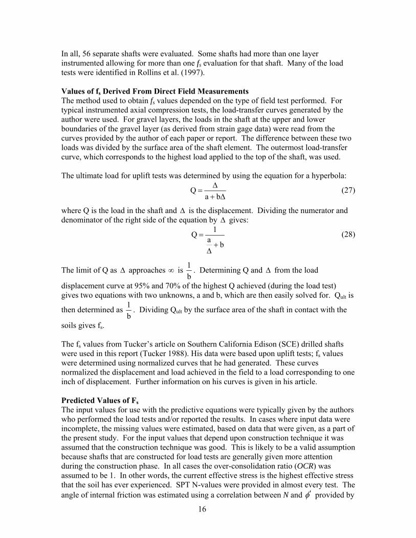
16
In all, 56 separate shafts were evaluated. Some shafts had more than one layer instrumented allowing for more than one fs evaluation for that shaft. Many of the load tests were identified in Rollins et al. (1997). Values of fs Derived From Direct Field Measurements The method used to obtain fs values depended on the type of field test performed. For typical instrumented axial compression tests, the load-transfer curves generated by the author were used. For gravel layers, the loads in the shaft at the upper and lower boundaries of the gravel layer (as derived from strain gage data) were read from the curves provided by the author of each paper or report. The difference between these two loads was divided by the surface area of the shaft element. The outermost load-transfer curve, which corresponds to the highest load applied to the top of the shaft, was used. The ultimate load for uplift tests was determined by using the equation for a hyperbola:
Qa b
Δ=
+ Δ (27)
where Q is the load in the shaft and Δ is the displacement. Dividing the numerator and denominator of the right side of the equation by Δ gives:
1Q a b=
+Δ
(28)
The limit of Q as Δ approaches ∞ is 1b
. Determining Q and Δ from the load
displacement curve at 95% and 70% of the highest Q achieved (during the load test) gives two equations with two unknowns, a and b, which are then easily solved for. Qult is
then determined as 1b
. Dividing Qult by the surface area of the shaft in contact with the
soils gives fs.
The fs values from Tucker’s article on Southern California Edison (SCE) drilled shafts were used in this report (Tucker 1988). His data were based upon uplift tests; fs values were determined using normalized curves that he had generated. These curves normalized the displacement and load achieved in the field to a load corresponding to one inch of displacement. Further information on his curves is given in his article. Predicted Values of Fs The input values for use with the predictive equations were typically given by the authors who performed the load tests and/or reported the results. In cases where input data were incomplete, the missing values were estimated, based on data that were given, as a part of the present study. For the input values that depend upon construction technique it was assumed that the construction technique was good. This is likely to be a valid assumption because shafts that are constructed for load tests are generally given more attention during the construction phase. In all cases the over-consolidation ratio (OCR) was assumed to be 1. In other words, the current effective stress is the highest effective stress that the soil has ever experienced. SPT N-values were provided in almost every test. The angle of internal friction was estimated using a correlation between N and φ′ provided by

17
Peck (1967) for the majority of cases where it was not provided. The angle of soil-pile interface was assumed to be equal to the angle of internal friction for all cases. Unit weights of the soils were estimated based on soil descriptions and the vertical effective stress was calculated using the typical procedure. The percentage of gravel was estimated using the soil descriptions and Rollins et al. (1997). It was not difficult in general to learn whether the soil was a sand, sandy gravel, or gravel.
Results The results are presented in the charts that follow. Figure 3 displays predicted versus actual fs for all of the predictive methods. Due to the assumptions made on the over-consolidation ratio, Tomlinson’s and Kulhawy’s methods yield the same results. Figure 4, Figure 5, Figure 6, and Figure 7 display the fs comparisons for each method with Tomlinson’s and Kulhawy’s shown on the same figure.
Predicted vs. Actual fs Values
02468
10
0 5 10
Actual [tsf]
Pred
icte
d [t
sf] Tomlinson and
KulhawyMeyerhoff
Reese & O'Neill
Rollins et al.
Figure 3. Predicted vs. Actual fs values, All Methods

18
Predicted vs. Actual fs Values Tomlinson and Kulhawy
02468
10
0 5 10
Actual [tsf]
Pred
icte
d [t
sf]
Tomlinson andKulhawy
Figure 4. Predicted vs. Actual fs Values, Tomlinson and Kulhawy
Predicted vs. Actual fs Values Meyerhoff
02468
10
0 5 10
Actual [tsf]
Pred
icte
d [t
sf]
Meyerhoff
Figure 5. Predicted vs. Actual fs Values, Meyerhoff

19
Predicted vs. Actual fs Values Reese & O'Neill
0
5
10
0 5 10
Actual [tsf]
Pred
icte
d [ts
f]
Reese & O'Neill
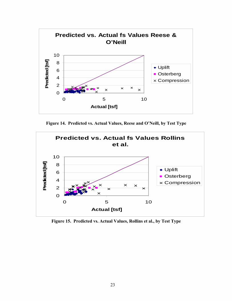
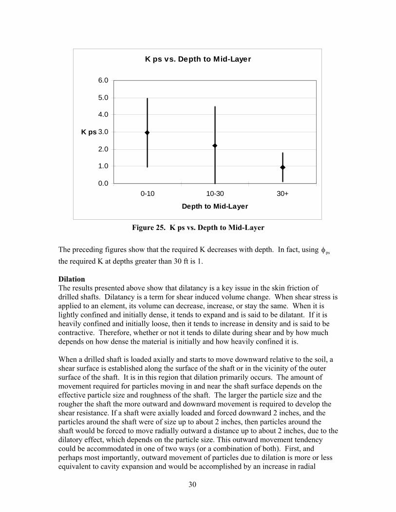
Figure 6. Predicted vs. Actual fs Values, Reese and O’Neill
Predicted vs. Actual fs Values Rollins et al.
02468
10
0 5 10
Actual [tsf]
Pred
icte
d [ts
f]
Rollins et al.
Figure 7. Predicted vs. Actual fs Values, Rollins et al. (1997)

20
There is a lot of scatter on the plots. In every case as the actual value of fs increases, the likelihood of a correct prediction decreases. The Rollins et al. (1997) method appears to offer the best correlation. To determine if a particular soil type is less likely to be accurately predicted than another, Figure 8, Figure 9, Figure 10, and Figure 11 differentiate between sands, sands w/gravels, and gravels.
Predicted vs. Actual fs Values Tomlinson and Kulhawy
0
2
4
6
8
10
0 5 10
Actual [tsf]
Pred
icte
d [ts
f]
SandSand/GravelGravel
Figure 8. Predicted vs. Actual Values, Tomlinson and Kulhawy, by Soil Type
Predicted vs. Actual fs Values Meyerhoff
0
2
4
6
8
10
0 5 10
Actual [tsf]
Pred
icte
d [ts
f]
SandSand/GravelGravel
Figure 9. Predicted vs. Actual Values, Meyerhoff, by Soil Type

21
Predicted vs. Actual fs Values Reese & O'Neill
0
2
4
6
8
10
0 5 10
Actual [tsf]
Pred
icte
d [ts
f]
SandSand/GravelGravel
Figure 10. Predicted vs. Actual Values, Reese and O’Neill, by Soil Type
Predicted vs. Actual fs Values Rollins et al.
0
2
4
6
8
10
0 5 10
Actual [tsf]
Pred
icte
d [ts
f]
SandSand/GravelGravel
Figure 11. Predicted vs. Actual Values, Rollins et al., by Soil Type

22
Gravels are the least likely to have fs accurately predicted. This is true for all methods. It appears that the modifications Rollins et al. make to the Reese and O’Neill method is sound for sand with gravel and still conservative for gravels. The Tomlinson and Kulhawy methods grossly under-predict all soil types while the Meyerhoff method offers a degree of predictability similar to Reese and O’Neill’s. There are three possible methods for testing the axial capacity of drilled shafts: Uplift, Osterberg, and Compression. Figure 12, Figure 13, Figure 14, and Figure 15 differentiate between the testing methods to determine if they have any influence on the results.
Predicted vs. Actual fs Values Tomlinson and Kulhawy
02468
10
0 5 10
Actual [tsf]
Pred
icte
d [ts
f]
UpliftOsterbergCompression
Figure 12. Predicted vs. Actual Values, Tomlinson and Kulhawy, by Test Type
Predicted vs. Actual fs Values Meyerhoff
02468
10
0 5 10
Actual [tsf]
Pred
icte
d [ts
f]
UpliftOsterbergCompression
Figure 13. Predicted vs. Actual Values, Meyerhoff, by Test Type
23
Predicted vs. Actual fs Values Reese & O'Neill
0
2
4
6
8
10
0 5 10
Actual [tsf]
Pred
icte
d [ts
f]
UpliftOsterbergCompression
Figure 14. Predicted vs. Actual Values, Reese and O’Neill, by Test Type
Predicted vs. Actual fs Values Rollins et al.
0
2
4
6
8
10
0 5 10
Actual [tsf]
Pred
icte
d [ts
f]
UpliftOsterbergCompression
Figure 15. Predicted vs. Actual Values, Rollins et al., by Test Type

24
The compression tests had the highest actual values of fs. Uplift tests had the lowest fs values while Osterberg tests fell in the middle. This is an interesting result and could imply that the test method does influence actual capacity determination. From the preceding graphs, it is obvious that the Rollins et al. (1997) method provides the best approximation of fs. The following graphs will examine the Tomlinson, Kulhawy, Meyerhoff, and Reese and O’Neill methods as one group and the Rollins et al. method as a second group. The first two figures, Figure 16 and Figure 17, take the predicted value of fs divided by the actual value of fs for the two groups described above, and compare the average to the percentage of gravel. The percentage of gravel represents the three soil types: sands, sands with gravel, and gravel. Because the percent of gravel associated with each computed value of skin friction was unknown, it was necessary to estimate these values from the soil descriptions corresponding to sands, sand with gravel and gravels. The values assigned were 20, 40, and 55 percent gravel, respectively. The uncertainty in the gravel percentages has no doubt contributed to the scatter in the computed values of the ratio of predicted to actual skin friction, P/A, and it is believed that the scatter would have been much less if the gravel percentage values had been measured and made available. However, the procedure adopted was essentially the only method available for approximately assessing the influence of gravel content on the skin friction. The point represents the average value of P/A and the line represents one standard deviation above and below the average P/A.
Average P/A vs. % Gravel All Methods sans Rollins et al.
0.00.2
0.40.60.81.0
1.21.4
20 40 55
% Gravel
Ave
rage
Pre
dict
ed/A
ctua
l
Figure 16. Average P/A vs. Percent Gravel, All Methods except Rollins et al.

25
Average P/A vs. % Gravel Rollins et al.
0.00.20.40.60.81.01.21.41.61.82.0
20 40 55
% Gravel
Ave
rage
Pre
dict
ed/A
ctua
l
Figure 17. Average P/A vs. Percent Gravel, Rollins et al.
Figure 16 displays the trend of decreasing predictability as the percentage of gravel increases for the first group of predictive methods. The actual value of fs for gravelly soils is under-predicted by an average of over 300%. For the Rollins method, Figure 17, the average values of P/A are much closer to 1 for the different soil types. Note that in the case of sands, which is the Reese and O’Neill method, the average P/A is very close to 1.

26
Figure 18 and Figure 19 examine the same groupings but this time versus depth to mid-layer. The depth to mid-layer was grouped into three depth intervals: 0-10 ft, 10-30 ft, and 30+ ft.
Average P/A vs. Depth to Mid-Layer All Methods sans Rollins et al.
0.0
0.2
0.4
0.6
0.8
1.0
0-10 10-30 30+
Depth to Mid Layer
Ave
rage
Pre
dict
ed/A
ctua
l
Figure 18. Average P/A vs. Depth to Mid-Layer, All Methods except Rollins et al.
Average P/A vs. Depth to Mid-Layer Rollins et al.
0.0
0.5
1.0
1.5
2.0
2.5
0-10 10-30 30+
Depth to Mid Layer
Ave
rage
Pre
dict
ed/A
ctua
l
Figure 19. Average P/A vs. Depth to Mid-Layer, Rollins et al.
For the first group, correlation between average P/A and depth to mid-layer is poor. The Rollins et al. group is better and the average values of P/A for depths greater than 10 ft are over-predicted.

27
Figure 20 and Figure 21 examine the same groups with respect to test type.
Average P/A vs. Test Type All Methods sans Rollins et al.
0.00
0.20
0.40
0.60
0.80
1.00
1.20
1.40
Compression Osterberg Uplift
Test Type
Ave
rage
Pre
dict
ed/A
ctua
l
Figure 20. Average P/A vs. Test Type, All Methods except Rollins et al.
Average P/A vs. Test Type Rollins et al.
0.00
0.50
1.00
1.50
2.00
2.50
Compression Osterberg Uplift
Test Type
Ave
rage
Pre
dict
ed/A
ctua
l
Figure 21. Average P/A vs. Test Type, Rollins et al.
Both figures display the same trend with the Rollins et al. method offset higher than the other group.

28
The next series of plots examines what the K value (from equation 14) would need to be to make the predicted value of fs match the actual value of fs. The vertical effective stress is determined from the soil profile while δ is set equal to φ . The value of φ is determined in one of two ways. The first is from SPT correlation as given by Peck et al. (1967: 310). The second method converts the φ found from the SPT correlation to a plane strainφ , or psφ, . The relationship between φ and psφ is: pssin tanφ = φ (29) Equation 29 is based on two assumptions: (1) the values of φ from the SPT correlation are more or less direct shear values, and (2) in the direct shear test the horizontal plane is not the “failure” plane but rather the point at the top of the corresponding Mohr’s circle. Setting fs equal to the actual value of fs, K is easily solved for. In Figure 22 the back-calculated K is based on φ . In Figure 23 the back-calculated K is based on φ ps and is denoted Kps. In figures 22 and 23, the back-calculated K values are plotted against the percentage of gravel or soil type.
K vs. % Gravel
0.0
2.0
4.0
6.0
8.0
10.0
12.0
20 40 55
% Gravel
K
Figure 22. K vs. Percent Gravel

29
K ps vs. % Gravel
0.0
1.0
2.0
3.0
4.0
5.0
6.0
20 40 55
% Gravel
K ps
Figure 23. Kps vs. Percent Gravel
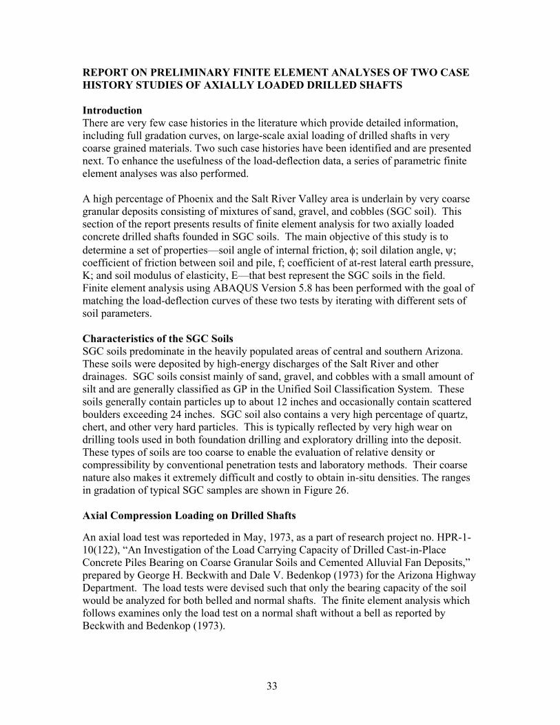
In both cases, the required K value increases as gravel content increases. Using psφ reduced the required K value for all cases by roughly half. Figure 24 and Figure 25 examine the required K values versus the depth to mid-layer.
K vs. Depth to Mid-Layer
0.0
2.0
4.0
6.0
8.0
10.0
12.0
0-10 10-30 30+
Depth to Mid-Layer
K
Figure 24. K vs. Depth to Mid-Layer
30
K ps vs. Depth to Mid-Layer
0.0
1.0
2.0
3.0
4.0
5.0
6.0
0-10 10-30 30+
Depth to Mid-Layer
K ps
Figure 25. K ps vs. Depth to Mid-Layer
The preceding figures show that the required K decreases with depth. In fact, using psφ the required K at depths greater than 30 ft is 1. Dilation The results presented above show that dilatancy is a key issue in the skin friction of drilled shafts. Dilatancy is a term for shear induced volume change. When shear stress is applied to an element, its volume can decrease, increase, or stay the same. When it is lightly confined and initially dense, it tends to expand and is said to be dilatant. If it is heavily confined and initially loose, then it tends to increase in density and is said to be contractive. Therefore, whether or not it tends to dilate during shear and by how much depends on how dense the material is initially and how heavily confined it is. When a drilled shaft is loaded axially and starts to move downward relative to the soil, a shear surface is established along the surface of the shaft or in the vicinity of the outer surface of the shaft. It is in this region that dilation primarily occurs. The amount of movement required for particles moving in and near the shaft surface depends on the effective particle size and roughness of the shaft. The larger the particle size and the rougher the shaft the more outward and downward movement is required to develop the shear resistance. If a shaft were axially loaded and forced downward 2 inches, and the particles around the shaft were of size up to about 2 inches, then particles around the shaft would be forced to move radially outward a distance up to about 2 inches, due to the dilatory effect, which depends on the particle size. This outward movement tendency could be accommodated in one of two ways (or a combination of both). First, and perhaps most importantly, outward movement of particles due to dilation is more or less equivalent to cavity expansion and would be accomplished by an increase in radial

31
normal stress as the particles are forced outward. If the material surrounding the shaft were of very low compressibility and densification could not be accommodated, then the ground surface would heave slightly to accommodate the dilation. In most cases it is expected that dilation is accommodated by both densification and heaving of the ground surface. The results of this study support the assertion of dilative behavior. The amount of dilation and corresponding increase in radial stress is expected to increase with the amount of gravel present in the soil, and the size of the gravel particles. With an increase in radial stress the skin friction capacity of the drilled shaft is expected to increase. The results clearly verified this phenomenon. As the depth increases, the confining pressure increases and the outward particle movement is accommodated by local densification around the shaft. Under these conditions the relative increase in radial stress is minimal and the K values tend to approach about 1.

32
Figure 26: Typical Grain Size Distribution of SGC Soil
33
REPORT ON PRELIMINARY FINITE ELEMENT ANALYSES OF TWO CASE HISTORY STUDIES OF AXIALLY LOADED DRILLED SHAFTS Introduction There are very few case histories in the literature which provide detailed information, including full gradation curves, on large-scale axial loading of drilled shafts in very coarse grained materials. Two such case histories have been identified and are presented next. To enhance the usefulness of the load-deflection data, a series of parametric finite element analyses was also performed. A high percentage of Phoenix and the Salt River Valley area is underlain by very coarse granular deposits consisting of mixtures of sand, gravel, and cobbles (SGC soil). This section of the report presents results of finite element analysis for two axially loaded concrete drilled shafts founded in SGC soils. The main objective of this study is to determine a set of properties—soil angle of internal friction, φ; soil dilation angle, ψ; coefficient of friction between soil and pile, f; coefficient of at-rest lateral earth pressure, K; and soil modulus of elasticity, E—that best represent the SGC soils in the field. Finite element analysis using ABAQUS Version 5.8 has been performed with the goal of matching the load-deflection curves of these two tests by iterating with different sets of soil parameters. Characteristics of the SGC Soils SGC soils predominate in the heavily populated areas of central and southern Arizona. These soils were deposited by high-energy discharges of the Salt River and other drainages. SGC soils consist mainly of sand, gravel, and cobbles with a small amount of silt and are generally classified as GP in the Unified Soil Classification System. These soils generally contain particles up to about 12 inches and occasionally contain scattered boulders exceeding 24 inches. SGC soil also contains a very high percentage of quartz, chert, and other very hard particles. This is typically reflected by very high wear on drilling tools used in both foundation drilling and exploratory drilling into the deposit. These types of soils are too coarse to enable the evaluation of relative density or compressibility by conventional penetration tests and laboratory methods. Their coarse nature also makes it extremely difficult and costly to obtain in-situ densities. The ranges in gradation of typical SGC samples are shown in Figure 26.
Axial Compression Loading on Drilled Shafts
An axial load test was reporteded in May, 1973, as a part of research project no. HPR-1-10(122), “An Investigation of the Load Carrying Capacity of Drilled Cast-in-Place Concrete Piles Bearing on Coarse Granular Soils and Cemented Alluvial Fan Deposits,” prepared by George H. Beckwith and Dale V. Bedenkop (1973) for the Arizona Highway Department. The load tests were devised such that only the bearing capacity of the soil would be analyzed for both belled and normal shafts. The finite element analysis which follows examines only the load test on a normal shaft without a bell as reported by Beckwith and Bedenkop (1973).

34
Soil Profile The soil profile for the first test consisted of roughly 7 feet of uncemented or weakly cemented silty clays and sandy clays underlain by moderate to strong lime-cemented clayey sands and sandy clays to a depth of 11 to 13.50 feet. Beneath this is a layer of moderately cemented clayey gravels; the SGC was first encountered between 14.5 to 16 feet, and it extended downward more than 20 feet according to Beckwith and Bedenkop (1973). The SGC layer is uncemented and relatively uniform except for a clean, fine to medium sand encountered at between 17.5 to 19 feet. In general, soil moisture contents were very low throughout the extent of the borings. Pile Configuration The reinforced concrete shaft had an average diameter of 2.50 feet and was 17.83 feet long. The top of the shaft was about 6 inches above the ground surface as shown in Figure 27. The side of the shaft was separated from the soil by a sonotube such that the test was strictly a measure of end-bearing capacity (frictionless shaft).
Figure 27: Pile Configuration Finite Element Analysis A finite element model was created using the ABAQUS Finite Element Program. The shaft was treated as a linear elastic material with modulus of elasticity, E, equal to 7.0×10⁸ pounds per square foot, and Poisson’s Ratio (υ) 0.30. The unit weight of the concrete is assumed to be 150 pounds per cubic foot. The soil is treated as an elastic fully-plastic material as repre-sented by the Drucker-Prager Model shown in Figure 28. The unit weight of the soil is assumed to be 125 pcf with a Poisson’s Ratio of 0.40. Sliding elements were installed between the shaft and the soil and have a coefficient of friction equal to zero to represent a frictionless shaft. A parametric study was done to study the effect of the soil internal angle of friction (φ), soil dilation angle (ψ), and soil modulus of elasticity (E), and to select opti-mum values. An associated flow rule was assumed first, such that the soil angle of internal friction equals the dilation angle. The field load-deflection curve is shown in Figure 29. Figure 30 shows the effect of soil modulus of elasticity (E) on the load deflection curve of
3 0 ``
6 ``
1 7 `-1 0 ``S o n otu b e

35
the axially loaded pier. The effect of the internal friction angle on the final load deflection curve is shown in Figure 31.
C
φ
τ
σ
φ
ψdεpl
Figure 28: Drucker-Prager Model.
0
100
200
300
400
500
600
700
800
900
1000
0 0.2 0.4 0.6 0.8 1 1.2 1.4 1.6 1.8 2
Displacement (in)
Load
(Ton
s)
Figure 29: Field Load-Deflection Curve.

36
0100200300400500600700800900
100011001200130014001500
0 0.5 1 1.5 2 2.5Displacement (in)
Load
(Ton
s)
TestE=0.4e7 psfE=1.25e7 psfE=2e7 psf
φ=36Ψ=36
Figure 30: Effect of Soil Modulus, E, on the Load Deflection Curve.
Figure 31: Effect of Soil Angle of Internal Friction, ø, on the Load Deflection Curve
0100200300400500600700800900
100011001200
0 0.5 1 1.5 2 2.5Displacement (in)
Load
(Ton
s)
Test
φ=30
φ=35
φ=37.5
φ=36
E=1.25e7 psfΨ=36

37
Effect of Dilation Angle Of course, the higher the dilation angle (ψ), the more the soil dilates. The ψ value should be less than or equal to the soil angle of internal friction (φ). A parametric study was performed to study the effect of dilation angle on the load deflection curve for the axially loaded drilled shaft. As an example of one of these sets of iterations, Figure 32 shows the effect of the dilation angle on the deflection curve for φ = 36o. Both φ and ψ were changed in such a way as to match the field load deflection curve as closely as possible. Figure 33 shows a summary of these trials and their comparison with the field test.
0100200300400500600700800900
100011001200
0 0.5 1 1.5 2 2.5Displacement (in)
Load
(Ton
s)
Testψ=36ψ=30ψ=40
E=1.25e7 psfφ=36
Figure 32: Effect of Soil Dilation Angle on Results.
0
100
200
300
400
500
600
700
800
900
1000
1100
1200
0 0.5 1 1.5 2 2.5
Displacement (in)
Load
(Ton
s)
Testφ=36, ψ=36φ=33, ψ=40φ=39, ψ=30φ=37.5, ψ=30φ=34.5, ψ=40φ=40, ψ=25φ=45, ψ=10φ=45, ψ=20φ=45, ψ=18
Figure 33: Set of Trials of Match Field Load-Deflection curve.

38
Best Fit Indicator The R2 value has been calculated using the Least Squares Method to correlate to the best fit of these results to the real field test. Figure 34 shows the R2 values for the different sets of finite element runs. Figure 35 shows the line representing the highest R2 values.
0
5
10
15
20
25
30
35
40
45
30 32.5 35 37.5 40 42.5 45 47.5
Soil Angle of Internal Friction, φ
Soil
Dila
tion
Ang
le, ψ
0.929 0.985
0.984
0.948 0.978 0.965
0.983
0.980.982
0.979
Figure 34: R2 Values for Different Sets of ø and Ψ
y = 549.44e-0.0765x
R2 = 0.9896
0
5
10
15
20
25
30
35
40
45
30 32.5 35 37.5 40 42.5 45 47.5
Soil Angle of Interanl Friction, φ
Dila
tion
Ang
le, ψ
Figure 35: Curve of Maximum R2 Values, for ψ vs φ.

39
Selection of Best Set of Parameters for SGC Based on the comparisons shown in figures 30 through 35 it was concluded that the best set of soil parameters for matching the field load-deflection curve for SGC is φ = 36o, for ψ = 36o, and E = 1.25 X 10⁷ psf. These values are associated with a unit weight of the soil of 125 pcf and Poisson’s ratio of 0.40. Uplift Loading on Drilled Shaft Test This test was reported in January, 1997, in Drilled Shaft Side Friction in Gravelly Soils, by Kyle M. Rollins, Robert J. Clayton, Rodney C. Mikesell, and Bradford C. Blaise for the Utah Department of Transportation (UT-97.02) (Rollins et al. 1997). The main objective of this test was to evaluate the side friction between the shaft and the soil generated by applying an uplift load on the shaft. This study is one of a very small number where sufficient data is available for back analysis. Soil Profile “A general description of the subsurface materials is as follows: from the ground surface to a depth of 12 feet -very dense coarse to fine gravel with cobbles; from 12 feet to the maximum depth of exploration (15 ft) - medium density sand. Percent gravel for the site ranges from 68% in the gravely materials to 2% in the silty sand. … Maximum particle size is 4 inches and ground water was encountered at 12.6 ft in the 15-foot shaft boring” (Rollins et al. 1997: 45). The grain size distribution for the soil at this site is shown in Figure 36. Additional specifics are given in Rollins et al (1997).
Figure 36: Grain size Distribution for the soil at Utah site.

40
Pile Configuration
The reinforced concrete pile had an average diameter of 2.00 feet and is 12.60 feet long as shown in Figure 37.
12.6`
24``
Very Dense Gravel with Brown to Dark Tan Sand and Cobbles
% Gravel=56 to 65%
Figure 37: Pile Configuration
Finite Element Analysis A finite element model was created using the ABAQUS Finite Element Program. The pile was treated like the last case study as a linear elastic material with modulus of elasticity, E, equal to 7.0×10⁸ psf, and a Poisson’s Ratio, υ, of 0.30. The unit weight of the concrete is assumed to be 150 pcf. The soil is also treated as an elastic fully plastic material represented by the Drucker-Prager Model as shown in Figure 28. The unit weight of the soil is assumed to be 125 pcf with a Poisson’s Ratio of 0.40. Friction elements were installed between the shaft and the soil. A parametric study was done to study the effect of the soil internal angle of friction (φ), soil dilation angle (ψ), coefficient of friction between soil and pile (f), and soil modulus of elasticity (E). The field load-deflection curve for the uplift load test is shown in Figure 38. Figure 39 shows the effect of soil modulus of elasticity, E, on the load deflection curve created by ABAQUS. The effect of the coefficient of friction between soil and pile, f, on the final load deflection curve is shown in Figure 40. Figure 41 shows the effect of the coefficient of at-rest lateral earth pressure, k, on the load deflection curve. From the above analysis, Figure 42 shows the best set of soil parameters for matching the field load-deflection curve. These parameters are: φ =42°, ψ=42°, E=2.25×10⁶ psf, k=2.8, and f=1.0.
The results of both sets of finite element analyses are expected to be useful in subsequent phases of the research project.
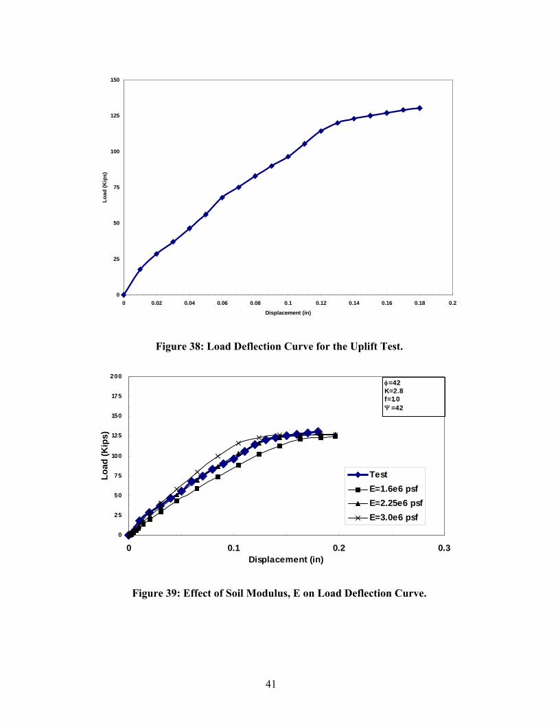
41
0
25
50
75
100
125
150
0 0.02 0.04 0.06 0.08 0.1 0.12 0.14 0.16 0.18 0.2
Displacement (in)
Load
(Kip
s)
Figure 38: Load Deflection Curve for the Uplift Test.
0
25
50
75
100
125
150
175
200
0 0.1 0.2 0.3Displacement (in)
Load
(Kip
s)
TestE=1.6e6 psfE=2.25e6 psfE=3.0e6 psf
φ=42K=2.8f=1.0Ψ =42
Figure 39: Effect of Soil Modulus, E on Load Deflection Curve.

42
0
25
50
75
100
125
150
175
200
0 0.1 0.2 0.3Displacement (in)
Load
(Kip
s)
Testf=0.70f=1.0f=1.50
φ=42E=2.25x10⁶ psfK=2.8Ψ=42
Figure 40: Effect of Coefficient of Friction between Pile and Soil, f.
0
25
50
75
100
125
150
175
200
0 0.1 0.2 0.3Displacement (in)
Load
(Kip
s)
Testk=2.5k=2.8k=3.0
φ=42E=2.25x10⁶ psff=1.0Ψ=42
Figure 41: Effect of Coefficient of Friction, f, on Load Deflection Curve.

43
0
25
50
75
100
125
150
175
200
0 0.1 0.2 0.3Displacement (in)
Load
(Kip
s)
Testk=2.8, f=1, E=1.1e5
Figure 42: Best Fit for the Uplift Load Test.
Conclusions from Study of Literature and Current Practice
None of the predictive methods for fine-grained material reported on herein work well for medium to high gravel content. All are extremely conservative at high drilled shaft capacity. Rollins et al. begins to address the issue but it would appear that a method specifically developed for gravelly soils is needed. It is relevant to note that the major source of error in these predictive methods from the literature is apparently the “K,” which is the ratio of horizontal normal stress to vertical normal stress. With the exception of the Rollins et al. (1997). procedure, essentially all the methods limit the K value to about 0.8. By contrast, Figures 16 through 25 show that the actual K ranges on average from about 1.5 to nearly 6, with the highest values being associated with shallow depth and high gravel content. Both conditions are associated with large radially-outward movements due to dilation. Even though the Rollins procedure produces more or less unbiased estimates of skin friction at low values of skin friction, the procedure greatly underestimates capacity when the skin friction is high.
As one studies each of these procedures, it typically appears that each author is
focused on assessing the K value just before the drilled shaft is constructed. No evidence exists that consideration was given to the buildup of K due to dilational behavior. In most instances it appears that the models were developed for smooth-wall driven shafts in fine-grained materials where dilational behavior was not an issue. It may well have not been the intention of the authors that their models be applied to gravelly materials.

44

45
DEVELOPMENT OF WORK PLAN FOR COMPLETION OF THE PROJECT AND ASSESSMENT OF PROGNOSIS FOR SUCCESS Data Gaps The impetus for SPR-493 came from ADOT and its consultants, who recognized the dearth of data on the drilled shaft capacity in very coarse materials with grain sizes up to that of SGC. They expressed concern that available design models from the literature for fine-grained materials that are in use today are far too conservative when used for very coarse-grained gravelly and cobbly materials and perhaps too conservative even for fine-grained materials in some cases. This report shows this concern is well justified. Given that the primary objective of SPR-493 was to develop a model for predicting the capacity of single and groups of drilled shafts in gravelly materials, including coarse gravels, it follows that potential data gaps would correspond to the data needed to develop and then to use the predictive model. A rather thorough literature review of methodologies for evaluating skin friction for drilled shafts has been conducted and the results of this review were reported in the “Summary of Literature and current Practice” section. These methodologies from the literature were combined with the experiences of the SPR-493 research team to develop a consensus on the most important parameters which influence the drilled shaft capacity and the form of a predictive model that would be practical for practitioners to use. This investigative process resulted in the conclusion that the most important parameters are:
1. Shear strength parameters of the material, φ′ (and c′ if material has significant cohesion).
2. Density of the material.
3. Dilational behavior of the material (specifically the amount of radially outward movement of particles which must occur to accommodate an increment of downward movement of the shaft).
4. Compressibility of the material as a function of effective stress state.
5. The grain size distribution (GSD) of the material.
Several of the above factors are interrelated; i.e., they are not independent. It is immediately obvious that even a modestly accurate evaluation of the above factors is not practical for practitioners engaged in routine design of drilled shafts. Therefore, the overall success of this research project requires that the above parameters be expressed as simple functions of one or two material index properties, so that evaluation of drilled shaft capacity can be easily accomplished. At this point in the research program it was tentatively concluded that only one index property would be required: the grain size distribution (GSD). It is believed that the other four parameters can be correlated, with satisfactory accuracy, with GSD. This is because we were persuaded that density could be related to GSD and the other parameters could then be related to density and/or GSD.
Because these correlations between GSD and the other 4 factors listed above had not yet been developed, this was an important first task in the next phase of this research. Correlations between grain size distribution (GSD), and each of the four factors:

46
1. c′ and φ′
2. Density
3. Dilational behavior
4. Compressibility obviously required that GSD be paired with each of these four factors so that correlations could be developed. The sources of data include (a) the literature, (b) the results of field in-situ density measurements and field sampling, and (c) the results of a lab test program performed at ASU as a part of SPR-493. The lab test program is described further under the heading “Lab Testing,” but here it is noted that it involves large scale direct shear tests on concrete/granular material interfaces. Each direct shear test series provides data on the relationships between GSD and φ′, dilational behavior, and compressibility. The relationship between GSD and density is derived from data obtained from the literature and from data gathered during visits to the field for sampling at gravelly material sites. In summary, the missing data needed to complete the SPR-493 study and develop a new model which can be used to predict drilled shaft capacity in gravelly materials are:
Pairs of values of GSD and a) c′, φ′ b) Density c) Dilational behavior d) Compressibility
Work Plan Overview This work plan entails field site investigations, laboratory testing, and analytical work including finite element simulations. It is aimed at development of a model for predicting drilled shaft axial load capacity in gravelly materials. Although some of the analyses conducted as a part of model development are rather sophisticated, the model finally developed is simple to use and employs input which is readily ascertained by practitioners. Because some background on the work plan was presented under the section “Data Gaps,” the tasks to be completed will be described very briefly.
Task 1- Site Visits for Sample Retrieval A wide variety of sites were visited to obtain data sets which relate GSD to material density. A second objective was to obtain samples for laboratory testing. Activities at each of these site visits included backhoe excavation to obtain representative samples and measure density. These pairs of values of GSD and density were used to develop a correlation between GSD and density.
Task 2- Laboratory Test Program The purpose of the laboratory test program was to generate data which can be used to relate GSD to:
1. c′, φ′ 2. Dilational behavior 3. Compressibility

47
The test apparatus and testing technique used are comprised of a large-scale (about 12 in square) direct shear apparatus which was used to measure compressibility, dilational response, and shearing resistance of concrete/material interfaces. This apparatus was designed and constructed at ASU. These tests were performed on a series of materials representing the full spectrum of gravelly materials. The percent gravel ranged from very small up to reasonably close to 100%. The materials included both well-graded and relatively uniform GSDs. The percent fines was typically less than 5. Each test series, for a material with a given GSD, included the following major steps:
1. Preparation/compaction to the density most typical of this GSD for naturally deposited materials in the field (using the correlations developed in Task 1).
2. Excavation/removal of half of the material—to be replaced with quickset concrete—while minimizing disturbance to the remaining material.
3. Casting of the concrete half of the test specimen, with the concrete being pressurized to a level typical of field placement conditions. This boundary condition is imposed to simulate as closely as possible the penetration into gravelly materials by the most liquid fractions of the concrete, which occurs in the field.
4. Application of confining pressure with measurement of compressibility of the gravelly material.
5. Shear to failure, with measurement of dilational response and measurement of shear resistance leading to c′ and φ′.
Task 3- Analysis and Model Development This task was necessarily iterative. The basic form of the predictive model used for skin friction, fs, and tip resistance, qtip, was
s vf c K tan′ ′ ′= + σ φ (30) where
• c′ and φ′ are effective stress strength parameters • v
′σ is the effective normal stress
• K is the ratio of horizontal normal stress to vertical normal stress
qtip = f(c′, φ′, compressibility, dilational response) The above forms of the predictive model were used during the conduct of the research. After completion of the research the practitioner/user will use greatly simplified predictive equations as follows:
( )s 1f f GSD,depth= (31)
( )tip 2q f GSD, depth= (32)

48
Thus the ultimate users of the model will need only grain size distribution (GSD) data as a material property as input. With only GSD data, the user can utilize a detailed step-by-step procedure for drilled shaft design, to arrive at a final design. The analyses under Task 3 proceeded somewhat as follows. The results from Tasks 1 and 2 were input to a Finite Element Model (FEM) which was used to predict the response of the drilled shaft to load. The FEM input parameters were adjusted to optimize agreement between prediction and measured results for as many as practical of the drilled shafts pre- sented under the section “Comparison of Actual Skin Friction Factors to Predicted for Drilled Shaft in Granular Soil.” The lateral stress ratio “K” was be evaluated from the FEM at all load levels. These finite element iterations were be used to develop the functions f1 and f2 cited above. At the end of the model development process we have a model that:
1. Is theoretically sound 2. Is overall consistent with available field drilled shaft test data 3. Can be used with only GSD data as input 4. Does not suffer from the ultra-conservatism exhibited by existing models.
Task 4- Development of a Design Methodology A design methodology was developed for the design of drilled shafts in gravelly materials. The methodology includes a detailed design example. Prognosis For Success It would, perhaps, be expected that the research team would be optimistic about the outcome of this effort even before the last half of the research work was completed. However, there were good reasons for this optimism. First, the approach proposed is fundamentally sound. The experimental and analytical phases were directed at identifying and evaluating fundamental material response parameters that are directly related to drilled shaft load capacity. To further illustrate the cause for optimism, the research team constructed a crude empirical model, based strictly on the data gathered under the “Summary of Literature and Current Practice.” This empirical model was constructed by combining the data in Figures 22 and 24 into one graph, using iterative adjustment to obtain smooth curves. The resulting combination is shown in Figure 43. The K value is the ratio of the horizontal to vertical stress as defined earlier. Likewise, the available database was used to very approximately relate density and φ′ value to percent gravel, P+4. These correlations shown in Figure 44 and Figure 45 are very approximate for several reasons, in particular the fact that P+4 was not typically reported in connection with the field drilled shaft test and had to be estimated from boring log material descriptions. These estimates contributed significantly to the scatter in the final results.

49
0
2
4
6
8
10
12
0 10 20 30 40 50 60Depth (ft)
K
55% = Percent Gravel = P+4
40%
20%
Figure 43: K vs Depth for different Gravel Content
105
110
115
120
125
130
20 25 30 35 40 45 50 55
% Gravel
γ (p
cf)
Figure 44: Gravel Content vs. Unit Weight, γ-Approximate Relationship

50
32
33
34
35
36
37
38
39
20 25 30 35 40 45 50 55
% Gravel
φ`
Figure 45: Gravel Content vs. φ` Value-Approximate Relationship
The values from Figure 43 through Figure 45 were used together with the estimated P+4 values and knowledge of the depth to estimate skin friction, fs by:
s vf K tan′ ′= σ φ (33)
These values of fs were then compared with the measured fs values to obtain Figure 46. Comparison of Figure 46 with Figure 3 shows that even this crude empirical model with all of its inherent approximations gives better agreement than any of the models found in the literature. The scatter in Figure 46 is still excessive and needs improvement; however, this was the starting point for the completion of the project. After the GSD and density at field locations are measured , the lab test results are received, and the analytical studies are completed, it would be quite reasonable to expect that a predictive model could be generated that exhibits much less scatter than that shown in Figure 46.

51
0
2
4
6
8
10
0 2 4 6 8 10
Measured (tsf)
Pre
dict
ed (t
sf)
Figure 46: Measured vs. Predicted for a New Empirical Model
The results presented up to this point present the findings from the survey of literature and current practice, the analyses of these literature findings, a report on preliminary finite element analyses of two axially-loaded drilled shafts, a work plan for completion of the project, and an assessment of the prognosis for success, together with a preliminary empirical model for K vs percent gravel and depth. The sections which follow present the results from newer work by the research team on field testing, laboratory work, finite element analyses, and development of a design model and design methodology.

52
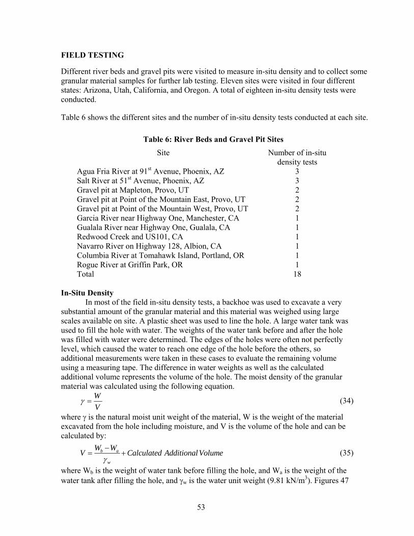
53
FIELD TESTING Different river beds and gravel pits were visited to measure in-situ density and to collect some granular material samples for further lab testing. Eleven sites were visited in four different states: Arizona, Utah, California, and Oregon. A total of eighteen in-situ density tests were conducted. Table 6 shows the different sites and the number of in-situ density tests conducted at each site.
Table 6: River Beds and Gravel Pit Sites Site Number of in-situ
density tests Agua Fria River at 91st Avenue, Phoenix, AZ 3 Salt River at 51st Avenue, Phoenix, AZ 3 Gravel pit at Mapleton, Provo, UT 2 Gravel pit at Point of the Mountain East, Provo, UT 2 Gravel pit at Point of the Mountain West, Provo, UT 2 Garcia River near Highway One, Manchester, CA 1 Gualala River near Highway One, Gualala, CA 1 Redwood Creek and US101, CA 1 Navarro River on Highway 128, Albion, CA 1 Columbia River at Tomahawk Island, Portland, OR 1 Rogue River at Griffin Park, OR 1 Total 18
In-Situ Density
In most of the field in-situ density tests, a backhoe was used to excavate a very substantial amount of the granular material and this material was weighed using large scales available on site. A plastic sheet was used to line the hole. A large water tank was used to fill the hole with water. The weights of the water tank before and after the hole was filled with water were determined. The edges of the holes were often not perfectly level, which caused the water to reach one edge of the hole before the others, so additional measurements were taken in these cases to evaluate the remaining volume using a measuring tape. The difference in water weights as well as the calculated additional volume represents the volume of the hole. The moist density of the granular material was calculated using the following equation.
=WV
γ (34)
where γ is the natural moist unit weight of the material, W is the weight of the material excavated from the hole including moisture, and V is the volume of the hole and can be calculated by:
−= +b a
w
W WV Calculated Additional Volumeγ
(35)
where Wb is the weight of water tank before filling the hole, and Wa is the weight of the water tank after filling the hole, and γw is the water unit weight (9.81 kN/m3). Figures 47

54
through 52 show photographs taken in the field illustrating the various tasks required for measuring the in-situ density.
Figure 47: Hole is Excavated Using the Backhoe.
Figure 48: The Material is Dumped (collected) in a Loader to be Weighed.
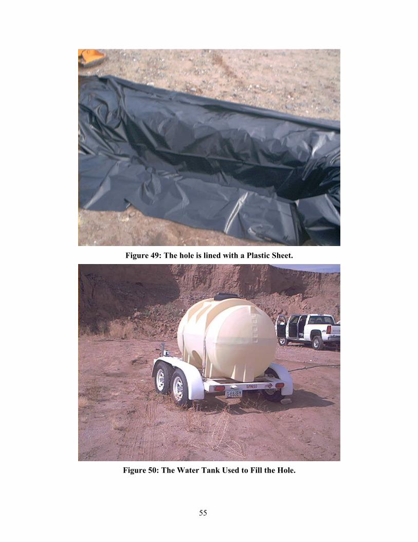
55
Figure 49: The hole is lined with a Plastic Sheet.
Figure 50: The Water Tank Used to Fill the Hole.

56
Figure 51: Hole Filled with Water.
Figure 52: Collected Samples

57
The material samples collected from the field were sealed as shown in Figure 52 to maintain the natural water content of each . Table 7 shows the moist in-situ density for each site. The moist in-situ density varied from a minimum value 104.6 pcf for the test at Columbia River, OR, to a maximum value of 148.5 pcf for the second test at 51st Avenue, Phoenix, AZ and the test at Rogue River, OR.
Table 7: Moist In-Situ Density Test No. Site Moist In-Situ Density (pcf)
1 91st Avenue (1) (AZ) 107.8 2 91st Avenue (2) (AZ) 139.9 3 91st Avenue (3) (AZ) 135.9 4 51st Avenue (1) (AZ) 144.1 5 51st Avenue (2) (AZ) 148.5 6 51st Avenue (3) (AZ) 135.0 7 Mapleton (1) (UT) 141.8 8 Mapleton (2) (UT) 144.0 9 Point of the Mountain East (1) (UT) 109.0 10 Point of the Mountain East (2) (UT) 112.0 11 Point of the Mountain West (1) (UT) 114.4 12 Point of the Mountain West (2) (UT) 109.8 13 Garcia River (CA1) 125.6 14 Gualala River (CA2) 116.3 15 Redwood Creek (CA3) 142.4 16 Navarro River (CA4) 120.2 17 Columbia River (OR1) 104.6 18 Rogue River (OR2) 148.5

58

59
LAB TESTING The lab testing can be divided into two main categories: first, grain size distribution and moisture content and second, large scale direct shear testing. Grain Size Distribution The material samples collected from the field were dried in an oven to measure the water content of each material. The water content for each test is shown in Table 8. The natural water content varied from 0.99% at Redwood Creek, CA to 7.31% at Columbia River, OR.
The dry material was sieved using large sieve shakers. The sieves ranged from 2 inches in size (5 cm) down to sieve #200 (0.074 mm). Occasionally it was necessary to measure a few very large particles manually. Figures 53 through 70 show the grain size distributions for the eighteen different material samples collected from the field. Figure 71 shows the grain size distribution curves for all materials on the same plot. The percentage of gravel varied from a minimum of 0% to a maximum of 82.1% as given in Table 9. The percentage passing the # 200 sieve varied from 0.13% for Redwood Creek, CA, to a maximum value of 5.05% for 51st Avenue, Phoenix, AZ.
Table 8: Natural Water Content
Material No. Site Water Content (%) 1 91st Avenue (1) 4.58 2 91st Avenue (2) 2.75 3 91st Avenue (3) 5.51 4 51st Avenue (1) 0.83 5 51st Avenue (2) 2.51 6 51st Avenue (3) 2.73 7 Mapleton (1) 2.74 8 Mapleton (2) 2.77 9 Point of the Mountain East (1) 2.14 10 Point of the Mountain East (2) 3.77 11 Point of the Mountain West (1) 2.90 12 Point of the Mountain West (2) 2.60 13 Garcia River (CA1) 2.15 14 Gualala River (CA2) 3.07 15 Redwood Creek (CA3) 0.99 16 Navarro River (CA4) 1.36 17 Columbia River (OR1) 7.31 18 Rogue River (OR2) 2.97

60
0102030405060708090
100
0.001 0.01 0.1 1 10 100Sieve Size (in)
Pass
ing
(%)
Figure 53: Grain Size Distribution for Material #1, 91st Avenue (1).
0102030405060708090
100
0.001 0.01 0.1 1 10 100Sieve Size (in)
Pas
sing
(%)
Figure 54: Grain Size Distribution for Material #2, 91st Avenue (2).
0102030405060708090
100
0.001 0.01 0.1 1 10 100Sieve Size (in)
Pas
sing
(%)
Figure 55: Grain Size Distribution for Material #3, 91st Avenue (3).

61
0102030405060708090
100
0.001 0.01 0.1 1 10 100Sieve Size (in)
Pas
sing
(%)
Figure 56: Grain Size Distribution for Material #4, 51st Avenue (1).
0102030405060708090
100
0.001 0.01 0.1 1 10 100Sieve Size (in)
Pas
sing
(%)
Figure 57: Grain Size Distribution for Material #5, 51st Avenue (2).
0102030405060708090
100
0.001 0.01 0.1 1 10 100Sieve Size (in)
Pass
ing
(%)
Figure 58: Grain Size Distribution for Material #6, 51st Avenue (3).

62
0102030405060708090
100
0.001 0.01 0.1 1 10 100Sieve Size (in)
Pas
sing
(%)
Figure 59: Grain Size Distribution for Material #7, Mapleton (1).
0102030405060708090
100
0.001 0.01 0.1 1 10 100Sieve Size (in)
Pas
sing
(%)
Figure 60: Grain Size Distribution for Material #8, Mapleton (2).
0102030405060708090
100
0.001 0.01 0.1 1 10 100Sieve Size (in)
Pas
sing
(%)
Figure 61: Grain Size Distribution for Material #9, Point of the Mountain East (1).

63
0102030405060708090
100
0.001 0.01 0.1 1 10 100Sieve Size (in)
Pas
sing
(%)
Figure 62: Grain Size Distribution for Material #10, Point of the Mountain East (2).
0102030405060708090
100
0.001 0.01 0.1 1 10 100Sieve Size (in)
Pas
sing
(%)
Figure 63: Grain Size Distribution for Material #11, Point of the Mountain West (1).
0102030405060708090
100
0.001 0.01 0.1 1 10 100Sieve Size (in)
Pas
sing
(%)
Figure 64: Grain Size Distribution for Material #12, Point of the Mountain West (2).

64
0102030405060708090
100
0.001 0.01 0.1 1 10 100Sieve Size (in)
Pas
sing
(%)
Figure 65: Grain Size Distribution for Material #13, Garcia River (CA1).
0102030405060708090
100
0.001 0.01 0.1 1 10 100Sieve Size (in)
Pas
sing
(%)
Figure 66: Grain Size Distribution for Material #14, Gualala River (CA2).
0102030405060708090
100
0.001 0.01 0.1 1 10 100Sieve Size (in)
Pas
sing
(%)
Figure 67: Grain Size Distribution for Material #15, Redwood Creek (CA3).

65
0102030405060708090
100
0.001 0.01 0.1 1 10 100Sieve Size (in)
Pas
sing
(%)
Figure 68: Grain Size Distribution for Material #16, Navarro River (CA4).
0102030405060708090
100
0.001 0.01 0.1 1 10 100Sieve Size (in)
Pass
ing
(%)
Figure 69: Grain Size Distribution for Material #17, Columbia River (OR1).

66
Figure 70: Grain Size Distribution for Material #18, Rogue River (OR2).
0
10
20
30
40
50
60
70
80
90
100
0.001 0.01 0.1 1 10 100Sieve Size (in)
Pass
ing
(%)
Test1 Test 2 Test 3 Test 4 Test 5 Test 6Test 7 Test 8 Test 9 Test 10 Test 11 Test 12Test 13 Test 14 Test 15 Test 16 Test 17 Test 18
Figure 71: Grain Size Distribution for All Materials.
010 20 30 40 50 60 70 80 90
100
0.001 0.01 0.1 1 10 100 Sieve Size (in)
Pass
ing
(%)

67
The primary gradation parameters, D10 up to D100, from each grain size distribution were determined and are shown in Table 9. The D10 values ranged from 0.004 in. for the first test at 91st Avenue, Phoenix, AZ, to a maximum value of 0.05 in. for the third test at 51st Avenue, Phoenix, AZ. However, D100 varied from 10 in. for the second test for the mate-rial at 91st Avenue, AZ, to a minimum of 0.25 in. for the material at Columbia River, OR.
Table 9: Various parameters of the Grain Size Distribution for All Samples.
Material No. D10 D20 D30 D40 D50 D60 D70 D80 D90 D100 P200 % Gravel1 0.004 0.006 0.008 0.012 0.015 0.026 0.053 0.081 0.524 4 5.05 17.05 2 0.009 0.026 0.062 0.226 0.501 1.168 2.405 5.502 9.138 10 4 59.1 3 0.015 0.037 0.058 0.085 0.217 0.319 0.463 0.866 1.423 5 1.657 47.46 4 0.028 0.063 0.292 0.645 1.061 1.502 2.098 2.828 5.162 7 0.57 71.66 5 0.030 0.057 0.132 0.368 0.856 1.337 1.910 2.632 4.923 8 0.608 64.74 6 0.053 0.313 0.640 0.897 1.140 1.385 1.714 2.175 2.780 6 0.202 82.1 7 0.021 0.065 0.282 0.476 0.717 0.989 1.374 1.951 2.657 8 0.848 72.1 8 0.006 0.015 0.206 0.393 0.637 0.941 1.311 1.783 2.384 3 1.67 69.3 9 0.010 0.019 0.035 0.051 0.068 0.116 0.228 0.348 1.274 7 1.56 28.02
10 0.007 0.013 0.025 0.047 0.069 0.196 0.337 0.642 1.504 3 2.88 37.47 11 0.077 0.014 0.026 0.040 0.054 0.068 0.101 0.194 0.303 2 3.677 13.96 12 0.009 0.015 0.024 0.036 0.048 0.060 0.072 0.119 0.216 1.5 1.613 6.44 13 0.020 0.036 0.053 0.319 0.442 0.621 0.836 1.140 1.524 3 1.23 67.16 14 0.030 0.049 0.068 0.104 0.162 0.220 0.284 0.357 0.574 3 0.366 34.7 15 0.033 0.062 0.134 0.277 0.486 0.822 1.200 1.682 2.549 5 0.134 61.72 16 0.013 0.045 0.088 0.139 0.190 0.241 0.357 0.068 0.498 2 0.74 38.1 17 0.007 0.009 0.011 0.013 0.015 0.021 0.037 0.053 0.069 0.25 1.07 0 18 0.044 0.210 0.593 1.042 1.468 1.880 2.261 2.631 3.000 6 0.642 78.97
All “D” are in inches.
A model for correlation between in-situ density and grain size distribution parameters of the granular material was developed using trial and error. The grain size distribution parameters D90/D10 and D50 were found to be the best parameters for a good correlation with the in-situ density. It was found that in-situ dry unit weight normalized to the unit weight of water could be correlated to the grain size distribution parameters as follows:
( )0.033
0.13439050 50
10
0.662 1.474 ,d
w
D D where D is in inchesD
γγ
⎛ ⎞= +⎜ ⎟
⎝ ⎠ (36)
( )0.033
0.13439050 50
10
0.662 0.9546 ,d
w
D D where D is in millimetersD
γγ
⎛ ⎞= +⎜ ⎟
⎝ ⎠ (37)
where γd is the in-situ dry unit weight and γw is the water unit weight (62.4 pcf or 9.81 kN/m3). The parameters D90, D50, and D10 are the particle sizes corresponding to 90, 50,
and 10 percent passing, respectively. The d
w
γγ
ratios measured from the field work were

68
compared to the d
w
γγ
ratios predicted from our model (equation 36) and the comparison is
shown in Figure 72. The predicted values from the model are adequately close to the measured ones, which indicates that the developed model is satisfactory for predicting the in-situ dry density for stream deposited granular materials from gradation data.
1.4
1.5
1.6
1.7
1.8
1.9
2.0
2.1
2.2
2.3
2.4
1.4 1.5 1.6 1.7 1.8 1.9 2.0 2.1 2.2 2.3 2.4Predicted (γd/γw)
Mea
sure
d (γ
d/ γw)
R2 = 0.90
Figure 72: Measured d
w
γγ
Values Versus Predicted
Large Scale Shear Testing A large scale shear box (1ftx1ftx1ft) was designed and built to test granular material (up to 2 inches particle size). Figure 73 shows a photograph of this device. The axial load (confining stress) was applied using four self-bottled hydraulic jacks, each of which has a 4 ton capacity. The lateral load (shear stress) was applied using two self-bottled hydraulic jacks, each of which has a 4 ton capacity. The shear load is applied on the upper half only while the lower half of the box is restrained using spacers placed between the box and the frame. The six jacks are connected to pressure gauges to read out the pressure. They were calibrated using load cells. The lateral deformation is measured using two dial gauges and the vertical deformation (compression or dilation) is measured using four dial gauges distributed to the corners of the box. The confining pressure jacks sit on steel bearings to minimize the friction between the jacks and the box.

69
Figure 73: Large Scale Shear Box
Testing Procedure
1. A certain amount of material remaining on each sieve was extracted to ensure that the gradation of each test specimen precisely matched the grain size distribution curve of each material. As shown in Figure 74, each layer of each test specimen was mixed dry in four different mixes and each compacted to the proper density.
2. An amount of water was added to each mix to match the water content in the field
as shown in Figure 74.
3. The material was compacted in four layers; each layer being 3 inches thick, as shown in Figure 75.
4. A cover plate was used to push the top layer flush with the box edges as shown in
Figure 76. This step ensures that the material is not over- or under-compacted and brings the density more or less precisely to the target value.

70
5. The box was flipped 90° to another side and half of the material was excavated as
shown in Figure 77. The gravel particles are almost never equidimensional. The longest dimension tends to be horizontal in the field. Therefore, in the field, the orientation of the particles is usually perpendicular to the axis of the drilled shaft. By flipping the box the gravel particles were oriented to be perpendicular to the concrete face, to be subsequently placed. Thus, to the extent possible, the “structure” of the gravel test specimen was matched to the expected field configuration.
6. Concrete was mixed using high cement content and an accelerator was used to
make it set up quickly and have a high strength. The upper half of the box was coated with Vaseline to make sure that the concrete would not stick to the steel plates and also to make it easy to extract the concrete block after the test. The concrete was then poured into the box as shown in Figure 78. Air pressure equal to the estimated overburden pressure was applied to the concrete face to represent the overburden pressure of the concrete at the depth of interest as shown in Figure 78.
7. After about two days, the concrete was adequately set up and the test specimen
was ready to be sheared. The box was lifted such that the concrete side was in the bottom half and the material side was in the upper half. The winch shown in Figure 73 was used to facilitate lifting and turning the filled shear box, which was quite heavy.
8. The upper steel plate (the one in contact with the material) was replaced by the
plate which carries the steel bearings and the four hydraulic jacks and which applies normal pressure.
9. The upper half of the box was then jacked up relative to the lower half to reduce
the friction between them. All six dial gauges (4 for axial deformations and 2 for lateral deformation) were then installed. Initial readings were taken for all gauges.
10. The confining pressure was first increased to a pressure equal to the overburden
pressure of concrete corresponding to the depth (section) under consideration. Next the confining pressure was adjusted to the target value (which could depend on the anticipated K value, which of course depends on depth and percentage of gravel).
11. The compressibility of the material was then determined from the increment(s) in
confining pressure described in previous steps.
12. This confining pressure was kept constant while applying the shear load. It was generally necessary to adjust the confining pressure jacks to keep the pressure constant, especially when dilation was large.
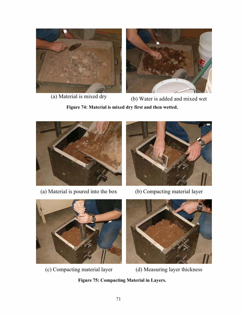
71
(a) Material is mixed dry (b) Water is added and mixed wet
Figure 74: Material is mixed dry first and then wetted.
(a) Material is poured into the box (b) Compacting material layer
(c) Compacting material layer (d) Measuring layer thickness
Figure 75: Compacting Material in Layers.

72
(a) Cover Plate into place. (b) Cover plate makes material flush
with box top.
Figure 76: A Cover Plate Used to Make Sure Material is Flush to Box Top.
Figure 77: Material is removed from the upper half of the box.

73
(a) Box Upper Half is Coated with Vaseline
(b) Concrete Poured from Mixer
(c) Concrete Poured into the Box
(d) Compacting Concrete
(e) Leveling Concrete
(f) Applying Air Pressure to Concrete
Figure 78: Pouring Concrete into the box.

74
Direct Shear Lab Test Program Six materials (out of the available eighteen) were chosen to be tested in the large scale direct shear box. They were chosen to cover a good range of percentage gravel and in-situ density. Table 10 shows these materials with their different configurations. The test matrix for all six materials is shown in Table 11. Each material was tested under three different confining pressures, and compressibility was measured. The shear stress versus lateral deformation was determined. The dilation response for each material was measured, as a function of gravel percentage and confining pressure.
Table 10: Properties of the Chosen Six Materials to be Tested in Large Scale Shear Box
Material No. γd (pcf) D10 D50 D90 D90/D10 P200 % Gravel 1 103.1 0.004 0.015 0.524 134.957 5.05 17.05 3 128.8 0.015 0.217 1.423 92.2132 1.657 47.46 7 138.0 0.021 0.717 2.657 126.524 0.848 72.1 9 106.7 0.099 0.068 1.274 12.8664 1.56 28.02 16 118.6 0.013 0.190 0.498 37.1493 0.74 38.1 17 97.5 0.007 0.015 0.069 10.0477 1.07 0
Table11: Large Scale Shear Box Test Matrix
Material No.
Confining Pressure (psf)
1 1185 2824 4345
3 1185 4345 7442
7 1185 4345 7442
9 1185 1934 4345
16 1185 2824 4345
17 418 1185 4345

75
Test Results Six materials were chosen from the complete set as representative of the full range of gradation and grain size distribution. These six were tested with large scale direct shear. All 18 grain size distribution curves are shown in Figures 53-57. Three different confining pressures, σ, were chosen for each material type as shown in Table 11. The load, P, versus lateral deformation, Δ, curves at three different confining pressures, σ, for each soil type are shown in Figure 79 through Figure 84.
Figure 79: Load Deflection Curve for Material #1.

76
0
500
1000
1500
2000
2500
3000
3500
4000
4500
0 0.05 0.1 0.15 0.2 0.25 0.3
Lateral Deformation, Δ (in)
Late
ral L
oad,
P (l
b) = 1185 psf =4345 psf =7442 psf
σσσ
Figure 80: Load Deflection Curve for Material #3.
0
1000
2000
3000
4000
5000
6000
0 0.05 0.1 0.15 0.2 0.25 0.3
Lateral Deformation, Δ (in)
Late
ral L
oad,
P (l
b)
= 1185 psf =4345 psf =7442 psf
σσσ
Figure 81: Load Deflection Curve for Material #7.

77
Figure 82: Load Deflection Curve for Material #9.
Figure 83: Load Deflection Curve for Material #16.

78
0
500
1000
1500
2000
2500
3000
0 0.05 0.1 0.15 0.2
Lateral Deformation, Δ (in)
Late
ral L
oad,
P (l
b) = 418 psf =1185 psf =4345 psf
σσσ
Figure 84: Load Deflection Curve for Material #17.
The shear strength envelope for each material tested is shown in Figure 85 through Figure 90. Figure 91 shows the summary of the shear envelops for the six tested materials.
0
500
1000
1500
2000
2500
0 1000 2000 3000 4000 5000
Confining pressure, σ (psf)
Shea
r Str
engt
h, τ
(psf
)
Figure 85: Shear Strength Envelope for Material #1.

79
0
500
1000
1500
2000
2500
3000
3500
4000
4500
0 1000 2000 3000 4000 5000
Confining pressure, σ (psf)
Shea
r Str
engt
h, τ
(psf
)
Figure 86: Shear Strength Envelope for Material #3.
0
1000
2000
3000
4000
5000
6000
7000
0 1000 2000 3000 4000 5000 6000 7000 8000
Confining pressure, σ (psf)
Shea
r Str
engt
h, τ
(psf
)
Figure 87: Shear Strength Envelope for Material #7.

80
0
500
1000
1500
2000
2500
3000
0 1000 2000 3000 4000 5000
Confining pressure, σ (psf)
Shea
r Str
engt
h, τ
(psf
)
Figure 88: Shear Strength Envelope for Material #9.
0
500
1000
1500
2000
2500
3000
3500
0 1000 2000 3000 4000 5000
Confining pressure, σ (psf)
Shea
r Str
engt
h, τ
(psf
)
Figure 89: Shear Strength Envelope for Material #16.
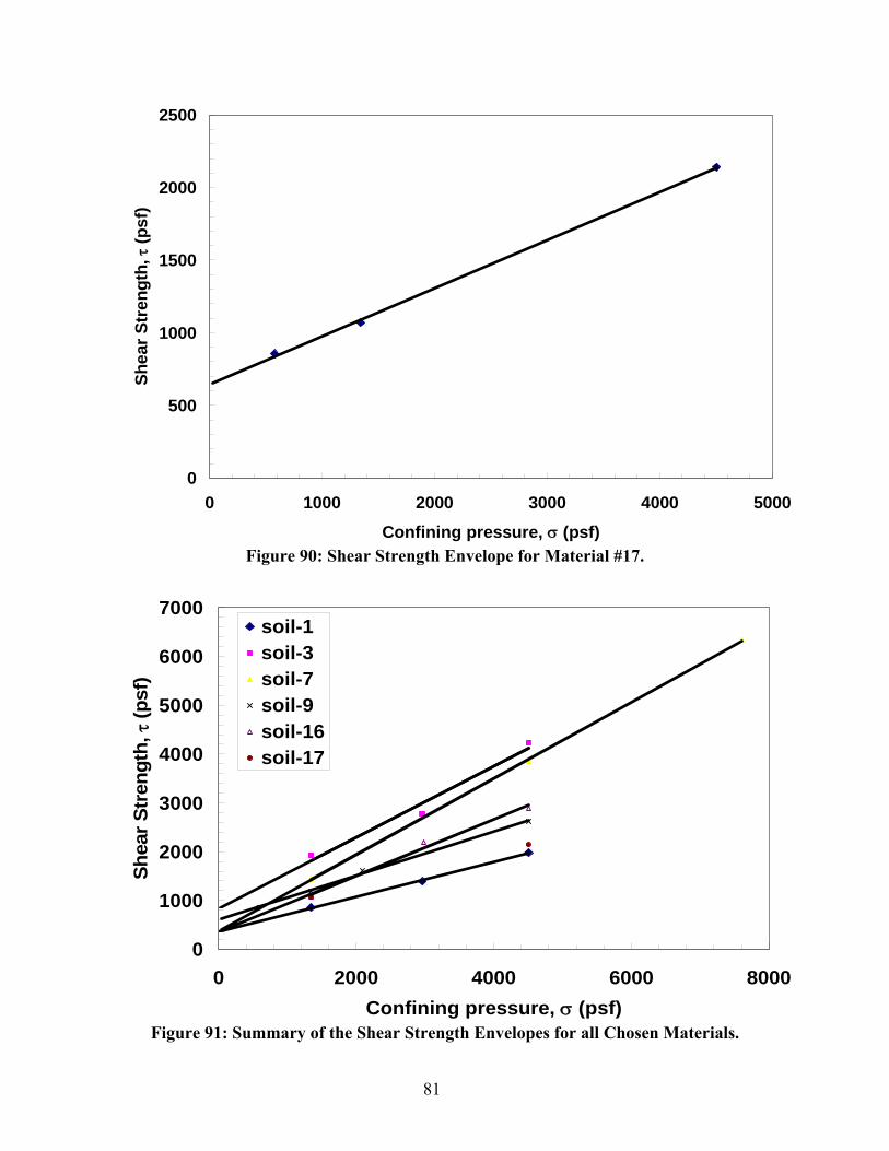
81
0
500
1000
1500
2000
2500
0 1000 2000 3000 4000 5000
Confining pressure, σ (psf)
Shea
r Str
engt
h, τ
(psf
)
Figure 90: Shear Strength Envelope for Material #17.
0
1000
2000
3000
4000
5000
6000
7000
0 2000 4000 6000 8000Confining pressure, σ (psf)
Shea
r Str
engt
h, τ
(psf
)
soil-1soil-3soil-7soil-9soil-16soil-17
Figure 91: Summary of the Shear Strength Envelopes for all Chosen Materials.

82
In figures 92-93, the lateral deformation was plotted against the vertical deformation for each soil at three different confining pressures. The dilation angle can be calculated as the average value of the arc-tan of the vertical deformation over the horizontal deformation.
Figure 92: Horizontal Deformation versus Vertical Deformation for Material #1.
0.00
0.02
0.04
0.06
0.08
0.10
0.12
0.14
0.16
0.18
0 0.05 0.1 0.15 0.2 0.25 0.3
Lateral Deformation, Δ (in)
Vertic
al D
efor
mat
ion,
δ (i
n)
=1185 psf =4345 psf =7442 psf
ψ = 27.9°σσσ
Figure 93: Horizontal Deformation versus Vertical Deformation for Material #3.

83
0.00
0.05
0.10
0.15
0.20
0 0.05 0.1 0.15 0.2 0.25 0.3
Lateral Deformation, Δ (in)
Vert
ical
Def
orm
atio
n, δ
(in)
=1185 psf =4345 psf =7442 psf
ψ = 31°σσσ
Figure 94: Horizontal Deformation versus Vertical Deformation for Material #7.
Figure 95: Horizontal Deformation versus Vertical Deformation for Material #9.

84
Figure 96: Horizontal Deformation versus Vertical Deformation for Material #16.
-0.01
0.00
0.01
0.02
0.03
0.04
0.05
0 0.05 0.1 0.15 0.2
Lateral Deformation, Δ (in)
Vert
ical
Def
orm
atio
n, δ
(in)
=418 psf =1185 psf =4345 psf
ψ = 3°σσσ
Figure 97: Horizontal Deformation versus Vertical Deformation for Material #17.
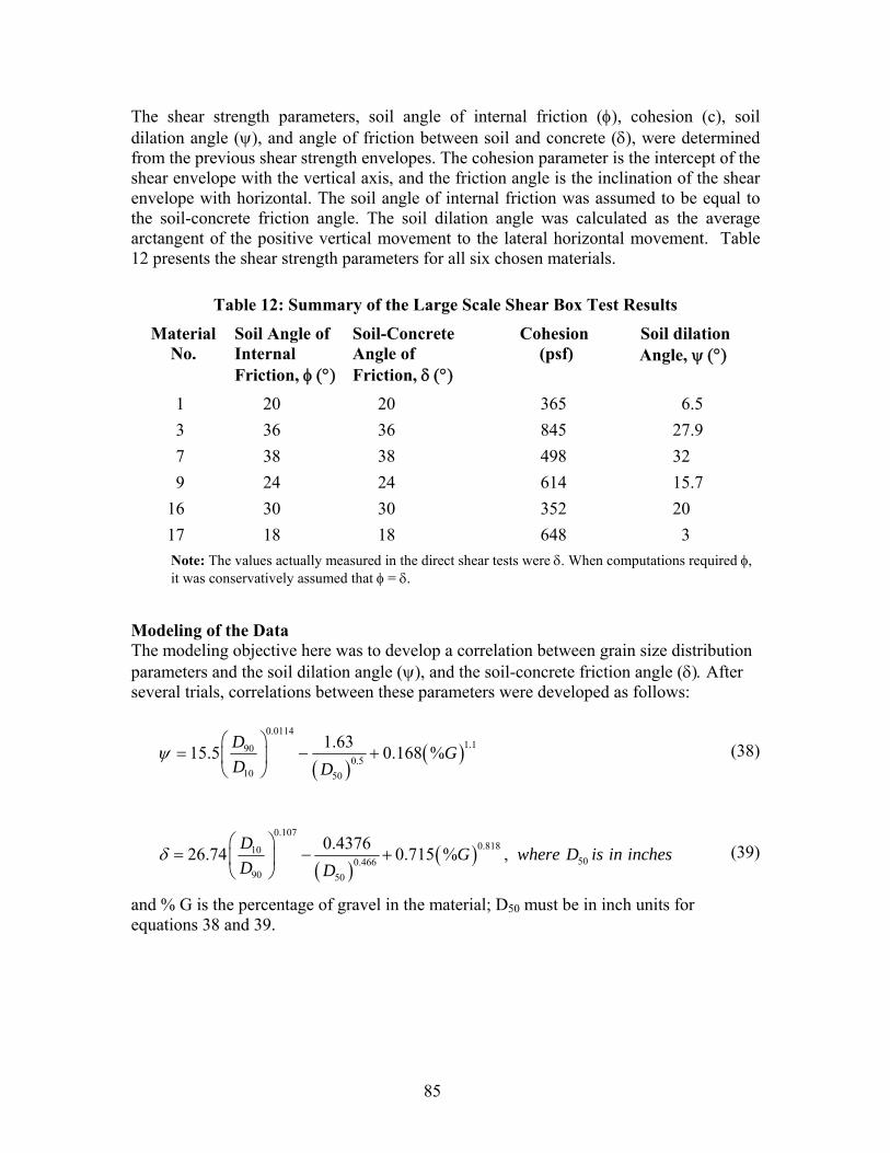
85
The shear strength parameters, soil angle of internal friction (φ), cohesion (c), soil dilation angle (ψ), and angle of friction between soil and concrete (δ), were determined from the previous shear strength envelopes. The cohesion parameter is the intercept of the shear envelope with the vertical axis, and the friction angle is the inclination of the shear envelope with horizontal. The soil angle of internal friction was assumed to be equal to the soil-concrete friction angle. The soil dilation angle was calculated as the average arctangent of the positive vertical movement to the lateral horizontal movement. Table 12 presents the shear strength parameters for all six chosen materials.
Table 12: Summary of the Large Scale Shear Box Test Results
Material No.
Soil Angle of Internal Friction, φ (°)
Soil-Concrete Angle of Friction, δ (°)
Cohesion (psf)
Soil dilation Angle, ψ (°)
1 20 20 365 6.5 3 36 36 845 27.9 7 38 38 498 32 9 24 24 614 15.7
16 30 30 352 20 17 18 18 648 3 Note: The values actually measured in the direct shear tests were δ. When computations required φ, it was conservatively assumed that φ = δ.
Modeling of the Data The modeling objective here was to develop a correlation between grain size distribution parameters and the soil dilation angle (ψ), and the soil-concrete friction angle (δ). After several trials, correlations between these parameters were developed as follows:
( )( )
0.01141.190
0.510 50
1.6315.5 0.168 %D GD D
ψ⎛ ⎞
= − +⎜ ⎟⎝ ⎠
(38)
( )( )
0.1070.81810
500.46690 50
0.437626.74 0.715 % ,D G where D is in inchesD D
δ⎛ ⎞
= − +⎜ ⎟⎝ ⎠
(39)
and % G is the percentage of gravel in the material; D50 must be in inch units for equations 38 and 39.
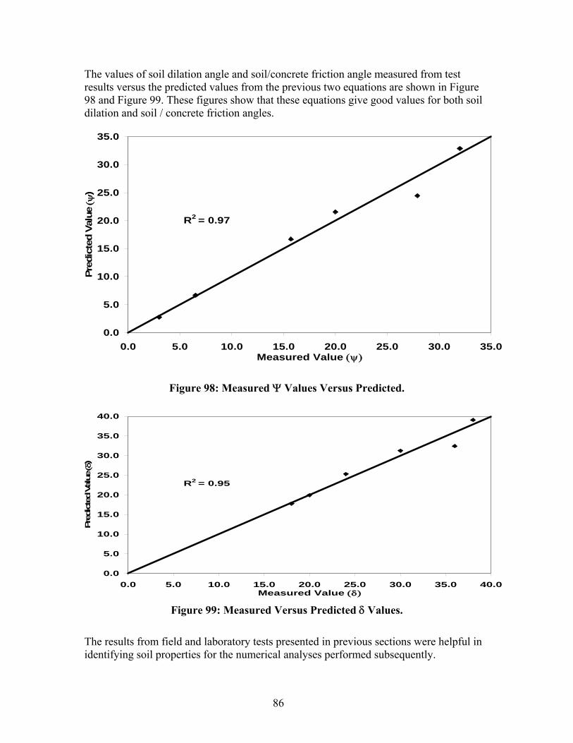
86
The values of soil dilation angle and soil/concrete friction angle measured from test results versus the predicted values from the previous two equations are shown in Figure 98 and Figure 99. These figures show that these equations give good values for both soil dilation and soil / concrete friction angles.
0.0
5.0
10.0
15.0
20.0
25.0
30.0
35.0
0.0 5.0 10.0 15.0 20.0 25.0 30.0 35.0Measured Value (ψ)
Pred
icte
d Va
lue
(ψ)
R2 = 0.97
Figure 98: Measured Ψ Values Versus Predicted.
0.0
5.0
10.0
15.0
20.0
25.0
30.0
35.0
40.0
0.0 5.0 10.0 15.0 20.0 25.0 30.0 35.0 40.0Measured Value (δ)
Pred
icte
d Va
lue
(δ)
R2 = 0.95
Figure 99: Measured Versus Predicted δ Values.
The results from field and laboratory tests presented in previous sections were helpful in identifying soil properties for the numerical analyses performed subsequently.

87
K Values From The Direct Shear Test
Given that K is defined as the ratio of the horizontal normal stress to the vertical normal stress it would appear on the surface that K cannot be measured from a direct shear test. However, if it is assumed that the following conditions exist, then K can be measured if the direct shear test progresses in increments, as it did for the tests done for this study.
1. Assume that the confining pressure initially applied represents the overburden
pressure at the particular depth being represented.
2. When the shear stress is increased, dilation ensues. However, for our tests this dilation is essentially inhibited by the stiffness of the oil in the hydraulic jacks applying the (normal) confining pressure. If it is assumed that the stiffness of the oil is comparable to the stiffness of the gravel surrounding the drilled shaft prototype, or at least sufficiently close in stiffness so as to have minor effect on the results, then the maximum normal stress generated by the dilation tendency divided by the initial value of the confining pressure would produce a K, similar to that developed in the prototype.
This excess normal pressure must be bled off before a set of readings is taken so the confining pressure returns to its initial value. It is noteworthy that if the confining pressure had been maintained constant with a pressure regulator, a servo device, or dead weights, this opportunity to infer a K value would not have been afforded. Thus, in these tests, the confining stress was only incrementally constant; that is, within the increment it did rise – in proportion to the dilation. For these tests the K values were evaluated as described above. K values for the last few increments (near failure) were averaged and plotted in Figure 108, to be presented subsequently.

88
Soil Finite Elements
Infinite (continuous) Soil Elements
Shaft Elements
Y X
Z
FIGURE 100: HALF SYMMETRY OF SHAFT AND SOIL DISCRETIZATION MESH

89
NUMERICAL ANALYSES Several finite element analyses were conducted to help in developing the final model to predict the skin friction values for drilled shaft foundations in gravelly soils. The finite element program ABAQUS was used for these analyses. Two different sites were picked where field test data on drilled shaft foundations in gravelly soils were available and also where the research team had visited and did field and lab testing on samples of these materials that had been returned to the laboratory. These two sites are Mapleton and Point of the Mountain East. The drilled shaft field load tests were done in January, 1997, at these two sites in Utah, as a part of research project UT-97.02, “Drilled Shaft Side Friction in Gravelly Soils.” The main objective of their tests was to evaluate the side friction between the shaft and the soil generated by applying an uplift load on the shaft. For each site we prepared the data required for each finite element run. The data included soil and shaft properties. The soil properties were: soil density (γ), soil angle of internal friction (φ), soil modulus of elasticity (Es), soil dilation (Ψ), Poisson Ratio (ν), and soil shaft friction angle (δ). The shaft parameters consist of shaft diameter (D), length (L), and modulus of elasticity (Ec). For all analyses we assumed that the Poisson Ratio to be 0.4 for soil and 0.3 for concrete. Equation 36 was used to predict the soil density (γ), and equations 37 and 38 to predict the soil dilation angle (Ψ), and soil shaft friction angle (δ). All of these equations utilize the soil grain size distributions which were available for each layer (different depths) in Rollins et al. (1997). Finite Element Model Finite element analyses, using the program ABAQUS (1998), were performed on a 3-D finite element model with 8-node elements. The boundary conditions include infinite (continuous) elements to reduce the effect of stress concentrations. The mesh shown in Figure 100 presents the results of several mesh refinement runs. In this mesh, the soil and shaft were discretized. The model consists of one single shaft with the load applied at the top of the shaft. The behavior of the reinforced concrete shaft was modeled as linear elastic. The soil was modeled as an elastic-perfectly-plastic, Drucker-Prager-Type material (Chen and Baladi, 1985), with volumetric dilation. Friction elements with a coefficient of friction (f), were used to represent the interaction between the soil and the shaft. A general description of the subsurface materials is as follows: from the ground surface to a depth of 12ft – very dense, coarse to fine gravel with cobbles; from 12ft to the maximum depth of exploration (15ft) – medium dense silty sand. The percent gravel for the site ranged from 68% in the gravelly material to 2% in the silty sand. Standard penetration blow counts range from 88 blows per 12 inches in the gravels to 11 blows per 12 inches in the silty sand. The reinforced concrete shaft had an average diameter of 24 inches and was 12.5 feet long.
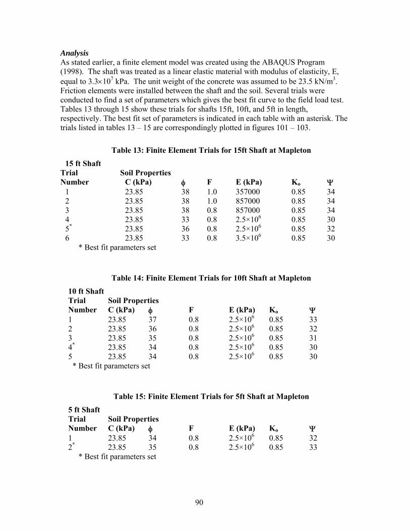
90
Analysis As stated earlier, a finite element model was created using the ABAQUS Program (1998). The shaft was treated as a linear elastic material with modulus of elasticity, E, equal to 3.3×10⁷ kPa. The unit weight of the concrete was assumed to be 23.5 kN/m3. Friction elements were installed between the shaft and the soil. Several trials were conducted to find a set of parameters which gives the best fit curve to the field load test. Tables 13 through 15 show these trials for shafts 15ft, 10ft, and 5ft in length, respectively. The best fit set of parameters is indicated in each table with an asterisk. The trials listed in tables 13 – 15 are correspondingly plotted in figures 101 – 103.
Table 13: Finite Element Trials for 15ft Shaft at Mapleton
15 ft Shaft Soil Properties Trial
Number C (kPa) φ F E (kPa) Ko Ψ 1 23.85 38 1.0 357000 0.85 34 2 23.85 38 1.0 857000 0.85 34 3 23.85 38 0.8 857000 0.85 34 4 23.85 33 0.8 2.5×10⁶ 0.85 30 5* 23.85 36 0.8 2.5×10⁶ 0.85 32 6 23.85 33 0.8 3.5×10⁶ 0.85 30
* Best fit parameters set
Table 14: Finite Element Trials for 10ft Shaft at Mapleton
10 ft Shaft Soil Properties Trial
Number C (kPa) φ F E (kPa) Ko Ψ 1 23.85 37 0.8 2.5×10⁶ 0.85 33 2 23.85 36 0.8 2.5×10⁶ 0.85 32 3 23.85 35 0.8 2.5×10⁶ 0.85 31 4* 23.85 34 0.8 2.5×10⁶ 0.85 30 5 23.85 34 0.8 2.5×10⁶ 0.85 30
* Best fit parameters set
Table 15: Finite Element Trials for 5ft Shaft at Mapleton
5 ft Shaft Soil Properties Trial
Number C (kPa) φ F E (kPa) Ko Ψ 1 23.85 34 0.8 2.5×10⁶ 0.85 32 2* 23.85 35 0.8 2.5×10⁶ 0.85 33
* Best fit parameters set

91
0
100
200
300
400
500
600
0.0 0.2 0.4 0.6 0.8 1.0Axial Deformation, Δ (in)
Axi
al L
oad,
P (K
ips)
Field Curve trial-1trial-2 trial-3trial-4 trial-5trial-6 trial-7
Best Fit
Figure 101: P-Δ Curves with Different Finite Element Trials for 15 ft Shaft at Mapleton
0
20
40
60
80
100
120
140
160
180
0.00 0.05 0.10 0.15 0.20 0.25Axial Deformation, Δ (in)
Axi
al L
oad,
P (K
ips)
Field Curvetrial-1trial-2trial-3trial-4
Best Fit
Figure 102: P-Δ Curves with Different Finite Element Trials for 10 ft Shaft at Mapleton

92
0
20
40
60
80
100
120
140
0.0 0.1 0.2 0.3 0.4 0.5Axial Deformation, Δ (in)
Load
, P (k
ips)
Field Curvetrial-1trial-2
Best fit
Figure 103: P-Δ Curves with Different Finite Element Trials
for 5 ft Shaft at Mapleton
Point of the Mountain East Site The subsurface materials generally are as follows: from the ground surface to a depth of 17ft – very dense, coarse to medium dense gravelly sand with silt; from 17ft to the maximum depth of exploration (20ft) – a dense layer of sand was found in the 10 foot shaft side, while a layer of dense fine gravel with sand and silt was found in the 5,15, and 20 foot shaft sites.. Percent gravel for the site ranges from 58% in the gravelly material to 4% in the sand with silt. Standard penetration blow counts range from 64 per 12 inches in the gravels to 15 per 12 inches in the sand layers. The reinforced concrete shaft had an average diameter of 24 inches and was 16.5 feet long. Tables 16 through 19 show the results for shaft lengths ranging from 5ft to 20ft. Again, the “Best Fit” parameters are indicated with an asterisk. The trials listed in tables 16 – 19 are correspondingly plotted in figures 104 – 107.
Table 16: Finite Element Trials for 5ft Shaft at Point of the Mountain East
5 ft Shaft Soil Properties Trial
Number C (kPa) φ f E (kPa) Ko Ψ 1 29.4 28 0.45 1.0×10⁶ 0.85 16 2 29.4 28 0.45 4.0×10⁵ 0.85 16 3 29.4 28 0.45 8.0×10⁵ 0.85 16 4* 29.4 28 0.45 9.2×10⁵ 0.85 16
* Best fit parameters set

93
Table 17: Finite Element Trials for 10ft Shaft at Point of the Mountain East
10 ft Shaft Soil Properties Trial
Number C (kPa) φ f E (kPa) Ko Ψ 1 29.4 26 0.45 9.2×10⁵ 0.85 13 2 29.4 35 0.45 9.2×10⁵ 0.85 19 3 29.4 30 0.45 9.2×10⁵ 0.85 18 4* 29.4 32 0.45 9.2×10⁵ 0.85 20
* Best fit parameters set
Table 18: Finite Element Trials for 15ft Shaft at Point of the Mountain East
15 ft Shaft Soil Properties Trial
Number C (kPa) φ f E (kPa) Ko Ψ 1 29.4 30 0.45 9.2×10⁵ 0.85 15 2 29.4 32 0.45 9.2×10⁵ 0.85 17 3 29.4 35 0.45 9.2×10⁵ 0.85 17 4 29.4 35 0.45 9.2×10⁵ 0.85 13 5* 29.4 30 0.45 9.2×10⁵ 0.85 18
* Best fit parameters set
Table 19: Finite Element Trials for 20ft Shaft at Point of the Mountain East
20 ft Shaft Soil Properties Trial
Number C (kPa) φ f E (kPa) Ko Ψ 1 29.4 25 0.45 9.2×10⁵ 0.85 14 2 29.4 28 0.45 9.2×10⁵ 0.85 18 3 29.4 32 0.45 9.2×10⁵ 0.85 20 4* 29.4 31 0.45 9.2×10⁵ 0.85 19
* Best fit parameters set
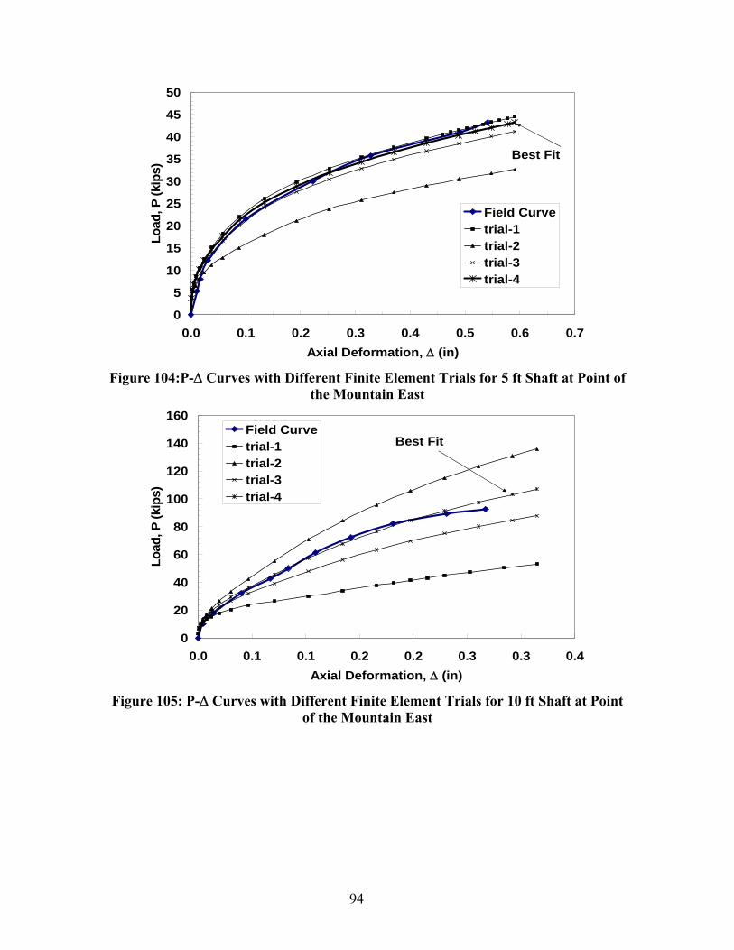
94
0
5
10
15
20
25
30
35
40
45
50
0.0 0.1 0.2 0.3 0.4 0.5 0.6 0.7Axial Deformation, Δ (in)
Load
, P (k
ips)
Field Curvetrial-1trial-2trial-3trial-4
Best Fit
Figure 104:P-Δ Curves with Different Finite Element Trials for 5 ft Shaft at Point of
the Mountain East
0
20
40
60
80
100
120
140
160
0.0 0.1 0.1 0.2 0.2 0.3 0.3 0.4Axial Deformation, Δ (in)
Load
, P (k
ips)
Field Curvetrial-1trial-2trial-3trial-4
Best Fit
Figure 105: P-Δ Curves with Different Finite Element Trials for 10 ft Shaft at Point
of the Mountain East

95
0
50
100
150
200
250
300
0.0 0.2 0.4 0.6 0.8Axial Deformation, Δ (in)
Load
, P (k
ips)
Field Curvetrial-1trial-2trial-3trial-4trial-5
Best fit
Figure 106: P-Δ Curves with Different Finite Element Trials for 15 ft Shaft at Point
of the Mountain East
0
50
100
150
200
250
300
350
0.0 0.1 0.2 0.3 0.4 0.5Axial Deformation, Δ (in)
Load
, P (k
ips)
Field Curvetrial-1trial-2trial-3trial-4
Best Fit
Figure 107: P-Δ Curves with Different Finite Element Trials for 20 ft Shaft at Point
of the Mountain East
K-Depth-% Gravel Model The results from lab and field tests as well as the results from numerical analyses (Finite Element Analyses) were used to compute the actual horizontal stress to vertical stress

96
along the shaft surface (K), with depth for different gravel contents and plotted in Figure 108. The continuous curves in Figure 108 represent the results from finite element analyses (stress ratio along the shaft surface for different gravel contents). The individual data points represent the results from the direct shear testing at a certain confining pressure (depth) for different gravel contents. The K values for the direct shear tests were determined as described in the preceding section. Given that the direct shear K values were based on rather dubious assumptions, it is quite remarkable that they plot essentially on the top of their respective finite element curves. Perhaps this is due in part to the fact that the direct shear and finite element K values are not entirely independent. A large number of the input parameters for the finite element runs were derived from the direct shear test results. Due to the fact that the direct shear K values did plot essentially on the top of the FE curves where they overlapped, the direct shear values were used to help extrapolate the FE curves (shown as small dashes) into deeper depth ranges.
Figure 108: K-Value versus Depth (From Finite Element and Direct Sheet)
It is also of interest to compare the K-Depth-%G model given by Figure 108 with the similar empirical model (Initial model) developed in Figure 43. This comparison is

97
shown in Figure 109. The curves from the strictly empirical model shown in Figure 43 are replotted in Figure 109 as dashed curves, with each curve labeled with its percentage of gravel (%G). No data points are shown for the empirical (Initial) model curves. Interpolation must be used to complete the comparison, but this interpolation shows that the agreement is quite close. These two sets of curves (the FE results and the empirical, initial model curves) were, in fact, totally independently derived.
Figure 109: Comparison between different methods used
to represent K-versus-%Gravel
In summary, the K-Depth-%G model presented in Figure 109 represents the confluence of three sets of data, all of which show very good agreement. Two of the sets, the FE and the empirical (Initial model) curves, are completely independent. Another two of the sets, FE and Direct Shear, are somewhat interdependent. However, given the very close agreement, the final model to be adopted would be the same, with or without the Direct Shear K values. Thus it is recommended that the Finite Element curves of Figure 108 be adopted for design and the proposed design procedure given in the next section is based on this K-Depth-%G model.

98

99
RECOMMENDED DESIGN PROCEDURES FOR DRILLED SHAFTS IN GRAVELLY MATERIALS
The procedure which follows is based on the findings and conclusions of the current study. Of course the findings of previous researchers, as cited in this report, were also relied upon. This procedure has been simplified so as to require only gradational data for each gravelly layer as input. Thus no laboratory or field testing is required, other than for gradation. The procedure is summarized in the following steps.
1. Divide the profile into layers within which the material properties can be assumed
to be constant. The last layer should extend down about 2D (two diameters) below the drilled shaft tip. The total number of layers should be between 4 and 12.
2. For each layer obtain the following gradation data: D90 (the diameter of the
material by which 90% is retained during sieve analysis), D50 (the diameter of the material by which 50% is retained during sieve analysis), D10 (the diameter of the material by which only10% is retained during sieve analysis), and the percent gravel (G(%)), which is the percent that will not pass through the No.4 sieve.
3. For each layer estimate the in-situ dry unit weight using Equation 36 or Equation
37.
( )0.033
0.13439050 50
10
0.662 1.474 ,d
w
D D where D is in inchesD
γγ
⎛ ⎞= +⎜ ⎟
⎝ ⎠ (36)
( )0.033
0.13439050 50
10
0.662 0.9546 ,d
w
D D where D is in millimetersD
γγ
⎛ ⎞= +⎜ ⎟
⎝ ⎠ (37)
4. For each layer, compute the effective overburden stress at the center of the layer
(σ′), and use Equation 39 to compute δ, the friction angle between the gravelly layer and the concrete shaft.
( )( )
0.1070.81810
500.46690 50
0.437626.74 0.715 % , ( )D
G where D is in inD D
δ⎛ ⎞
= − +⎜ ⎟⎝ ⎠
(39)
A limiting maximum value of 43° is recommended for δ = φ .
5. For each layer, obtain K—the ratio of the horizontal normal stress to the vertical normal stress—from Figure 108 using the depth to the midpoint of each layer. Interpolate as required for percent gravel (% G) value of the layer.
6. Compute the unit skin friction (fs), for each layer as:
δσ tan′= Kfs

100
7. Compute the skin friction contribution to the drilled shaft load capacity (Qs), for each layer, by:
Qs each layer = fs × skin area within the layer
8. Compute the total skin friction load capacity as the summation of all the
contributions of the layers from the shaft tip to the surface.
9. The total obtained in step 8 represents an ultimate skin friction value. Since design is normally controlled by allowable deflection, it is therefore necessary to apply a factor of safety to the ultimate skin friction to control the deflection. The load-deflection curve for drilled shaft skin friction is nonlinear and fairly well represented by a hyperbola. The experience of the authors from their own research and consulting and the collected experience of others, as given by the literature (Rollins et al. 2005) were used to develop the following recommendations for the relationship between factor of safety and deflection.
Table 20: Factor of Safety vs. Deflection for Drilled Shaft Skin Friction Factor of Safety, FSSK
Δ/D = Ratio of Deflection to Shaft Diameter
Stress Level = Q/Qult×100 =100/FSSK
1.0 ≈ 0.04 100 1.35 0.013 74 1.5 0.01 67 2.0 0.005 50 3.0 0.0026 33 4.0 0.002 25
In Table 20 deflection is given as a ratio of deflection, Δ, to shaft diameter, D. To complete step 9, tentatively choose a value of Δ likely to be acceptable, compute Δ/D where D corresponds to an initial trial design shaft diameter, enter Table 20 and interpolate to get a FSSK.
10. Divide the ultimate skin friction from step 8 by the FSSK from step 9: ( ) ( ) SKskinskin FSultimateQdesignQ /=
11. Compute a qp (ultimate) and multiply by the area of the shaft tip to get Qp
(ultimate). These sub steps are:
a) Use Equation 7 to get (qp)ult:
( ) qultp Nq σ ′= (7)
where σ` is the effective overburden stress at the center of the last material layer. This center point would be 1D below the shaft tip, if the layer thickness

101
was 2D, and Nq = the bearing capacity factor from the Berezantsev bearing capacity curves in Figure 2. The φ value with which the bearing capacity curves are entered is the δ value from Equation 39
( )( )
0.1070.81810
500.46690 50
0.437626.74 0.715 % ,D G where D is in inchesD D
δ⎛ ⎞
= − +⎜ ⎟⎝ ⎠
(39)
The value of δ for this and all other layers was computed in step 4 above, as were the σ′ values. The assumption that δ = φ will typically be slightly conservative. Recall from Step 4 that δ = φ is limited to a maximum value of 43°.
b) (qp)ult × Area of shaft tip = (Qp)ult
12. Apply a factor of safety (FS) for the tip of the shaft, FSp, to get (Qp)design =
(Qp)ult/FSp. The FSp is obtained from Table 21 below. The relationship between FSp and Δ/D for the tip (Table 21) is different from the relationship given in Table 20 for the skin friction because the normalized load-deflection curves are different for the skin friction and tip resistance. However, for balanced and consistent design, Table 21 should be entered with the same Δ/D that was chosen for design and used to enter Table 20.
Table 21: Factor of Safety vs. Deflection for Drilled Shaft Tip Resistance
Factor of Safety, FSp Δ/D = Ratio of Deflection to shaft Diameter
Stress Level = Q/Qult×100 =100/FSp
1.0 ≈0.1 100 1.5 0.035 67 2.0 0.02 50 2.5 0.013 40 3.3 0.008 30 5.0 0.005 20
Further reduction in Qp (design) is left to the discretion of the user. If, for example, inspection of the drilled shaft hole bottom shows that it was very poorly cleaned, further reduction in Qp (design) may be warranted. If the compression of any relatively soft material under the shaft can be estimated, then this estimate can be subtracted from the Δ value chosen in step 9 to obtain a new, net Δ, corresponding to the deflection of the actual underlying bearing layer. This new, net Δ can then be used to get a new, net Δ/D with which Table 21 can be entered to get a new (higher) FSp. As the net Δ approaches zero or goes negative it is prudent, of course, to neglect the point load contribution altogether.

102
13. Add Qsk (design) from step 10 to Qp (design) from step 12 to get Qtotal (design): Qtotal (design) = Qsk (design) + Qp (design)
14. Compare the Qtotal (design) from step 13 with the Q to be applied by the
superstructure. If Qtotal (design) from step 13 is adequate and about right, the foundation design process is complete at this point. If, however, Qtotal (design) is inadequate, then adjustments must be made in the design to increase the load-carrying capacity. Examples of such adjustments are (1) accepting a larger deflection, Δ, (2) increasing the diameter of the shaft(s) and (3) increasing the length (depth) of the shaft(s). If Qtotal (design) is well in excess of the capacity needed, make adjustments to reduce Qtotal (design), such as reducing the shaft diameter or length.
After making any adjustment to the design it is then necessary to iterate through steps 1 through 14 until Qtotal (design) is adequate and about right.
Comparison of the Ultimate Tip Resistance by Equation 7 using Berezantsev Bearing Capacity Factors with the Measured Tip Resistance for the Beckwith and Bedenkop Test on Salt River SGC
The available case histories that can be used to compare the actual measured point load with that predicted using the procedure outlined in step 11 above are very few indeed. However, one such case history is available and it is the Beckwith-Bedenkop Test on SGC presented and analyzed in this report. The load-deflection curve for this test is given in Figure 29 and shows that the Qult value is just over 1000 tons, at a deflection of about 2.2 inches. The shaft diameter is 30 inches and the length is about 17.5 ft. Thus Δ/D at the ultimate condition is about 0.073, and (qp)ult (measured) is just over 204 tsf. The gradation curves shown in Figure 26 show a range in gradation for SGC, from which the following gradation parameters were chosen:
D90 = 2” D50 = 0.6” D10 = 0.02” (G%) = 70%
Using Equation 39 - as in step 11 – the δ value is computed as 39º:
( )( ) °=+−⎟
⎠⎞
⎜⎝⎛= 3970715.0
6.04376.0
202.074.26 808.0
466.0
107.0
δ (39)
In Figure 2 the curves are labeled with values of D/B. Note that the nomenclature is different for Figure 2 compared to the usage herein. In Figure 2, D = shaft length and B = least width. In this report, when Δ/D is evaluated, D is used as the shaft diameter. For entering Figure 2 with δ = φ = 39º, a D/B ratio of 17.5’/2.5’ = 7 is used. The Berezantsev curves yield Nq = 153. The value of σ′ is given by:
σ′ = (17.5+2.5) × 131 pcf = 2620 psf, for pore pressure = 0

103
Average values of γd = 122 pcf and γtotal = 131 pcf were used, using Equation 7 as in step 11,
(qp)ult (predicted) = 153 × 2620 = 400860 psf = 200 tsf
which agrees very closely with the (qp) ultimate measured of 204 tsf.
A large database from which measured and predicted (qp)ult values could be compared is not available at the present time. If it were, however, it is likely that such good agreement, as for the case above, would not necessarily be typical. Therefore, it is of course prudent to apply a FSp to the (qp)ult, as outlined in step 12. Note, however, that the FSp being applied in step 12 is primarily for the purpose of controlling deflection. The probability of a plunging-type bearing capacity failure is quite low for FSp as low as 2, or even 1.5.

104

105
EXAMPLE DRILLED SHAFT DESIGN, USING THE RECOMMENDED PROCEDURE
For purposes of illustrating the procedure a profile with 6 layers of thicknesses as shown in Table 22 has been arbitrarily chosen. In this example Material Layer Nos. 1, 3, and 4 happen to correspond to Materials Nos. 1, 7, and 3, respectively, in Table 9. The GSD data and G (%) values for the other Material Layer Nos. of Table 22 were chosen totally arbitrarily. For the first iteration of the trial design a shaft of 3’ in diameter and 30’ in length has been chosen. The results from steps 1 and 2 are combined in Table 22 below.
Steps 1 and 2
Table 22: Results from Steps 1 and 2 – Example Design
Material Layer No.
Layer Thickness, ft
Depth to Mid-point, ft
D90, in
D50, in
D10, in
G (%)
1 5 2.5 0.524 0.015 0.004 17 2 7 8.5 0.25 0.012 0.0035 10 3 6 15 2.657 0.717 0.021 72.1 4 5 20.5 1.423 0.217 0.015 47.5 5 7 26.5 1.65 0.23 0.017 50 6* 6 33 0.574 0.162 0.03 34.7
layer 6 is below the shaft tip
Steps 3, 4, and 5 The results for steps 3, 4, and 5 are combined in Table 23 below:
Table 23: Results from Steps 3, 4, and 5 – Example Design Material Layer No.
(a) γd, pcf
(b) * moist unit weight, pcf
( c ) effective overburden stress, σ`, psf
(d) δ = φ deg
(e) ** K value
1 100.8 103.8 260 20 2.6 2 98.3 101.2 873 18 1.65 3 136.4 140.5 1649 39 7.5 4 122.9 126.6 2386 32.4 4.4 5 123.5 127.2 3148 33 3.6 6 117.6 121.1 3956 31.5 ----
*based on an assumed average moisture content of 3.0% ** from Figure 108. Note: the K value for layer 6 is not obtained because it is not
used.

106
Take layer 3 as an example:
(a) ( )
( ) pcfd
w
d
4.1364.62186.2
186.2717.0474.1021.0657.2662.0 143.0
033.0
=×=
=+⎟⎠⎞
⎜⎝⎛=
γγγ
(b) ( ) ( ) pcfdm 5.1404.13603.103.1 =×=×= γγ
(c) ( )( ) ( )( ) ( )( ) psf16495.14032.10178.1035 =++=′σ (assuming pore pressure = 0)
(d) ( )( )
°=
+−⎟⎠⎞
⎜⎝⎛=
39
1.72715.0717.0
4376.0657.2021.074.26 818.0
466.0
107.0
δ
(e) Enter Figure 108 with depth = 15` and G(%) = 72.1 to get K = 7.5
Steps 6, 7, and 8 The results for steps 6, 7, and 8 are combined in Table24 below:
Table 24: Results from Steps 6, 7, and 8 – Example Design
Material Layer No.
σ` psf
δ degrees
K fs tsf
Skin area, Ask (ft2)
Qs tons
1 260 20 2.6 0.123 47.1 5.8 2 873 18 1.65 0.234 65.96 15.4 3 1649 39 7.5 5.00 56.5 282.5 4 2386 32.4 4.4 3.33 47.1 156.8 5 3148 33 3.6 3.68 65.96 242.7 6 3956 31.5 ---- ----- ----- -----
Summation = Qsk (ultimate) 703.2
Step 9 Assume Δ = 0.35`` is selected as a target deflection. For D = 36``, Δ/D = 0.35/36 ≈ 0.01. Entering Table 20 with 0.01, the indicated FSsk = 1.5.
Step 10 Qsk (design) = Qsk (ultimate)/FSsk Qsk (design) = 703 tons / 1.5 = 469 tons

107
Step 11 Use (qp)ult = σ′Nq
σ′ = 3956 psf at a depth of 33’`, which is 1D beneath the tip of the drilled shaft. Assume φ = δ =31.5º and enter Figure 2 with 31.5º. Berezantsev’s D/B = 30/3 = 10; therefore, Nq = 32. (qp)ult = 3956 (32) = 126,592 psf = 63.3 tsf Area of tip = πD2/4 = 7.07 ft2. ∴(Qp)ult = 63.3 tsf × 7.07 ft2 = 447.5 tons Step 12 A value of Δ/D = 0.01 was used to enter Table 20 and should likewise be used to enter Table 21. Thus FSp = 2.82 is to be applied to (Qp)ult. (Qp) (design) = (Qp)ult / FSp = 447.5 tons / 2.82 (Qp) (design) = 158.7 tons Assume hole bottom was “clean” and the full 158 tons will be used. Step 13 (Qtotal) (design) = Qsk (design) + Qp (design) (Qtotal) (design) = 469 tons + 158 tons = 627 tons Step 14 The Qtotal (design) from step 13 is 627 tons. Table 25 below shows various hypothetical values of Q applied by the superstructure and the associated indicated action.
Table 25: Comparison of Qtotal (design) and Q applied by the Superstructure and Indicated Actions
Qtotal (design) (tons)
Qapplied (tons)
Indicated Action
627 600 Design is adequate. No further iteration 627 620 Design is probably adequate; no further iteration 627 800 Design is inadequate. Adjust to increase capacity and iterate 627 400 Design is excessively conservative; adjust to decrease capacity and iterate

108

109
CONCLUSIONS
As of the completion of the Summary of Literature and Current Practice, it was tentatively concluded that the presence of large amounts of gravel in a material would contribute to dilation during shear, which in turn would contribute to development of higher lateral stress during loading. The higher lateral stress is expressed as a higher K value, where K is the ratio of lateral to vertical stress. The exhibition of dilation and high K values with large amounts of coarse gravel was confirmed by the studies herein, especially the large scale direct shear tests for which dilation was measured directly and K values were inferred. These findings were also confirmed with the Finite Element Analyses, which yielded K values from the stress state of the elements adjacent to the drilled shaft. The K-depth-% G model shown in Figure 108 and the comparison in Figure 109 of (1) the entirely empirical (Initial) model for K-depth-% G of Figure 43 and (2) the K-values inferred from large-scale direct shear measurements and (3) the K-values derived from FE studies show close agreement between all three sets of the K-values. This close agreement heightens confidence in the final model adopted and depicted in Figure 108. The K-values found for gravelly materials range up to 8 or 9 times – for shallow depth and high gravel content – the corresponding K-values for fine grained materials. Values of K of 2 to 4 times those for fine grained material models are very common. Comparison between measured and predicted skin friction using fine grained models showed that the fine grained models under-predicted the measured skin friction by a factor of 2 to 8 when the gravel content of the material was moderate to high. These comparisons should not be interpreted as a criticism of the developers of the fine grained models because the models were developed and calibrated for fine-grained materials. They have been used subsequently for gravelly material simply by default because a more appropriate model has not been available. Their use in the past for gravelly materials has been conservative, though this conservatism has been very costly. This study has led to a better understanding of the reasons and mechanisms by which the K-values are so much higher for gravelly materials than for fine grained materials. First, the presence of significant gravel leads to more dilation during shear, including larger outward (radial) particles movements as the drilled shaft is loaded. Secondly, and perhaps more importantly, materials with large amounts of gravel are much less compressible than fine grained materials, up to an order of magnitude less compressible in some cases. Thus, much more lateral stress is built up during shear, for a given amount of dilation. Finally, it should be noted that some of the fine grained skin friction models seem to have been focused on the stress state in the material either just before the drilled shaft is installed or just after, whereas, the stress state which is most important in governing skin friction is the one which develops during loading, after the dilation that is going to occur has occurred. Because the high K-values depicted in Figure 108 and Figure 109 represent values directly derived from field load tests, as well as those inferred from direct shear tests and
110
computed from FE analyses, it is recommended that the associated design procedure for drilled shafts in gravelly soils be adopted. This procedure is well-founded on reality and is relatively simple and practical to use. Because the procedure uses correlations between needed parameters and gradation data it can be implemented quickly at relatively low cost. It is recommended that bucket augers be used to get disturbed but representative samples for gradation testing. If the exploratory holes are advanced with an impact hammer which crushes the larger gravel and rock fragments, it may possible to approximate the percent of gravel and to roughly approximate a corresponding “best guess” gradation curve. However, the parameters derived from these more approximate processes will be degraded somewhat and the accuracy of the corresponding computed drilled shaft capacity will likewise be degraded somewhat. It should be noted that Figure 108, which yields K-value is entered only with percentage of gravel and the K-value is the value which most strongly controls the design. The GSD is used to estimate in-situ dry unit weight and the δ angle, and eventually the tip resistance. It is therefore recommended that bucket augers be used, or any method which preserves the gradation data.

111
REFERENCES
AASHTO see American Association of State Highway and Transportation Officials American Association of State Highway and Transportation Officials. 1998. AASHTO LRFD Bridge Design Specifications.2nd ed. Washington, DC: American Association of State Highway and Transportation Officials. Baker, C. N., Jr., G. Parikh, J.-L. Briaud, E. E. Drumright, and F. Mensah, 1993. Drilled Shafts for Bridge Foundations. Report No. FHWA-RD-92-004. Washington, D.C.: Federal Highway Administration. Beckwith, George H. and Dale V. Bedenkop. 1973. An Investigation of the Load Carrying Capacity of Drilled Cast-in-Place Concrete Piles Bearing on Coarse Granular Soils and Cemented Alluvial Fan Deposits. Report No. AHD-RD-10-122. Phoenix, AZ: Arizona Highway Dept. Berezantsev, V. G. 1961. "Load-bearing Capacity and Deformation of Piled Foundations." in Proceedings of the 5th International Conference on Soil Mechanics. 2: 11-12. Paris: Dunod. Chen, W. F and G. Y. Baladi. 1985. Soil Plasticity: Theory and Implementation. New York: Elsevier. Chua, K. M. and W. A. N. Aspar. 1993. Application of Pile Driving Analyzer: Final Report. Santa Fe, N.M.: New Mexico State Highway and Transportation Dept. Frank, R., N. Kalteziotis, M. Bustamante, S. Christoulas, and H. Zervogiannis. 1991. "Evaluation of Performance of Two Piles Using Pressuremeter Method." Journal. of Geotechnical Engineering 117(5) 695-713. Fujioka, T. and K. Yamada, K. 1994. “The Development of a New Pile Load Testing System.” Proceedings, International Conference on Design and Construction of Deep Foundations 2: 670–684. Washington, D.C.: Federal Highway Administration. Hansen, J. B. 1961. A General Formula for Bearing Capacity. Danish Geotechnical Institute Bulletin No. 11. Copenhagen: Danish Geotechnical Institute. (see also the following by Hansen) Hansen, J. B. 1968. A Revised Extended Formula for Bearing Capacity. Danish Geotechnical Institute Bulletin No. 28. Copenhagen: Danish Geotechnical Institute.
112
Hansen, J. B. 1978. Code of Practice for Foundation Engineering. Danish Geotechnical Institute Bulletin No. 32. Copenhagen: Danish Geotechnical Institute. Konstantinidis, B., A. J. Pacal, and A. W.Shively. 1987. “Uplift Capacity of Drilled Piers in Desert Soils: A Case History.” In Foundations for Transmission Line Towers: Proceedings of a Session, ed. J.-L. Briaud, 128–141. Geotechnical Special Publication No. 8. New York: American Society of Civil Engineers.
Kulhawy, F. H. 1991. "Drilled Shaft Foundations." in Foundation Engineering Handbook. 2nd ed., ed. H.Y. Fang, 537-551. New York: Van Nostrand Reinhold. Matsui, T. 1993. “Case Studies on Cast-in-Place Bored Piles and Some Considerations for Design.” In Proceedings of the 2nd International Geotechnical Seminar on Deep Foundations on Bored and Auger Piles, ed. W. F. VanImpe, 77-102. Rotterdam, The Netherlands: Balkema. Meyerhoff, G.C. 1976. "Bearing Capacity and Settlement of Pile Foundations." Journal of the Geotechnical Engineering Division 102(GT3): 197-228. . Peck, R. B., W. E. Hanson, and T. H. Thornburn.1967. Foundation Engineering. 2nd ed. New York: John Wiley. Price, R., K. M. Rollins, and E. Keane. 1992. “Comparison of Measured and Computed Drilled Shaft Capacities Based on Utah Load Tests.” Transportation Research Record 1336: 57–64. Reese, L. C. and M. W. O'Neill.1989. "New Design Method for Drilled Shafts from Common Soil and Rock Tests." in Foundation Engineering: Current Principles and Practices, ed F. Kulhawy. 2:1026-1039. New York: American Society of Civil Engineers. Rollins, K. M., R. J. Clayton, R. C. Mikesell, and B. C. Blaise. 1997. Drilled Shaft Side Friction in Gravelly Soils. Report No. UT-97.02. Salt Lake City: Utah Dept. of Transportation. Rollins, K. M., R. J. Clayton, R. C. Mikesell, and B. C. Blaise. 2005. “Drilled Shaft Side Friction in Gravelly Soils.” Journal of Geotechnical and Geoenvironmental Engineering 131(8): 987-1003. Tomlinson, M. J. 2001. Foundation Design and Construction. 7th ed. London: Prentice Hall. Tucker, K. D. 1987. “Uplift Capacity of Drilled Shafts and Driven Piles in Granular Materials.” In Foundations for Transmission Line Towers: Proceedings of a Session, ed. J.-L. Briaud, 142–159. Geotechnical Special Publication No. 8. New York: American Society of Civil Engineers..

113
Tucker, K. D. 1988. “Performance Evaluation of Pile Foundation using CPT Data.” In Proceedings of the 2nd International Conference on Case Histories in Geotechnical Engineering, ed. by Shamsher Prakash, 1355-1364. Rolla, MO: Univ. of Missouri-Rolla.