dual economies, kaldorian underemployment and the big...
TRANSCRIPT

Dual economies, Kaldorian underemployment and
the big push
Giovanni Valensisi∗
October 2007
This paper develops a two-sector model with speci�c factors of production, featuring
diminishing returns and standard wages in agriculture, while increasing returns and
e�ciency wage mechanisms in industry. The asymmetric interaction of the two sectors
is such that, under plausible parametrization, the model may display multiple equilibra
and a low-development trap. Additionally, parametric increases of sectoral TFP may
reduce the basin of attraction of the low-equilibrium and increase the steady state capital
stock (and wage level) for the stable equilibrium of full industrialization.
I. Introduction
The concept of poverty trap has been used fruitfully since the very dawn of devel-opment economics, and implicitly it can be traced back even to Adam Smith's "Earlydraft of part of the Wealth of Nations"1. Starting with the seminal paper of RosensteinRodan (1943), the idea that underdevelopment could constitute a state of equilibriumthrived with Nurkse's vicious circle of poverty (1953) and Nelson's low-level equilibriumtrap (1956). Several mechanisms, essentially concerning increasing returns pecuniary ex-ternalities or demographic traps, were from time to time held responsible for creatinga multiplicity of equilibra, and possibly preventing the spontaneous development ofcertain economies2.
∗Dipartimento di Economia Politica e Metodi Quantitativi; University of Pavia;([email protected]). II am gratefully indebted to Gianni Vaggi, Marco Missaglia, Amit Bhaduri, Jaime Ros, Paolo Berto-letti, Carluccio Bianchi and Mario Cimoli for their helpful comments. I also bene�tted from thesuggestions of Alberto Botta, Francesco Bogliacino, Luca Mantovan, Lorenza Salvatori, ChiaraValensisi, Francesco Magalini and Sara Baroud. The responsibility of remaining errors is of coursemine.
1In Smith (1763) page 579 the author argues:
"That is easier for a nation, in the same manner as for an individual, to raise itself from a moderate
degree of wealth to the highest opulence, than to acquire this moderate degree of wealth."2Authors such as Young (1928), Rosenstein-Rodan (1943) and Nurkse (1953) emphasized the im-
portance of increasing returns, while Nelson (1956), Jorgenson (1964) and - later - Dixit (1970) focused
on the role of demographic dynamics in creating poverty traps, in which economic growth in absolute
terms is balanced by the counteracting dynamics of population, so that GDP per capita remains at a
2 Giovanni Valensisi
Despite the deep interest enjoyed by the so-called "high development theory" in the�fties, its predominantly discursive argumentation jointly with the di�culty to reconcileincreasing returns with competitive market structures3 contributed to its decline infavor of the more rigorous paradigm, described by Solow (1956) and Swan (1956).Notwithstanding many important contributions on the role of increasing returns andlearning by doing, during the 60's the mainstream approach to growth became that ofthe neoclassical convex economy converging to a stable and unique steady state.
Additionally, attention shifted from the "developmental perspective" - emphasiz-ing the interactions between "sectoral balances" (in terms of labor, goods and saving�ows) along the process of industrialization, as well as the dualistic nature of theeconomies of developing countries - to an aggregate growth perspective - focusing moreon reproducible factors' accumulation, and on the determinants of the steady state.In this respect, the use of a linearly homogeneous aggregate production function re-quires great caution, because of the subtle but delicate implications of such choice interms of positive theory4. More importantly, the choice of an aggregate model over-looks the empirically-founded recognition that economic growth goes hand in handwith structural change, meaning that "the permanent changes in the absolute levels ofbasic macro-economic magnitudes are invariably associated with changes in their com-position, that is, with the dynamics of their structure"5. Obviously, the importanceof structural dynamics is reinforced a fortiori, when referring to developing economiesthat are undergoing a process of industrialization.
Regardless of the possible limits of aggregate models, also the mainstream approachhas played a key role in bringing back to the center of the attention the issue of in-creasing returns, along with their crucial implications for multiple equilibra. The twistaway from the traditional paradigm of conditional convergence occurred in the mid80's, when endogenous growth theory stressed the role of knowledge and human capi-tal, be it a sort of separate product (di�erent from the composite good) or simply thestock of experience and learning by doing. The assumption of increasing returns to re-producible factors, where the latter typically include knowledge, in addition to physicalcapital, responded to the need to rationalize two elements of industrial economies thatwere basically assumed exogenously in Solow's conceptual framework: the persistence ofgrowth even after the capital labor ratio has reached fairly high levels, and the continu-ity (or possibly even the acceleration) of technical change. In light of this, endogenousgrowth theory was mostly concerned with issues other than explaining the take o� ofinitially poor countries, consequently it focused more on the properties of the steady
low level.3Notably during the 50's and 60's only demographic traps had been analyzed in mathematical form,
while poverty traps based on increasing returns, specialization and pecuniary externalities were treated
only in narrative contributions.4Solow himself recognized the di�culty to apply a linearly homogeneous aggregate production
function to both agriculture and industry. The point is raised in two di�erent articles: Solow (1956)
page 67 cautions about applying an aggregate production function, which is linearly homogeneous, to
the case in which production depends on a "nonaugmentable resource like land"; Solow (1957) page 314
states the need to net out agricultural contribution to GDP when applying the aggregate production
function to the analysis of real economies.5The quotation is taken by Pasinetti (1993), italics in the original.

Dual economies, Kaldorian underemployment and the big push 3
state path, rather than on the possible obstacles to industrialization. This di�erent rai-son d'etre also explains why early endogenous growth models featured predominantlya one sector or "quasi-one-sector" set-up6, omitting by de�nition any possible role forlabor reallocation and structural change.
In any case, in the mid 90's concepts like poverty traps, structural change andmultiplicity of equilibra recovered a central role in the debate about economic growth,leading to what has been called a "counter-counterrevolution in development theory"7.On the one hand, it had been shown that even in the standard neoclassical set-up(one sector with convex technologies operating under perfect competition), multipleequilibra cannot be excluded a priori once empirically signi�cant elements such asheterogeneity in saving behavior, low elasticity of technical substitution, or capitalmarket imperfections are taken into account8. On the other hand, advances in thetheoretical analysis of non-perfectly competitive market structure, jointly with a newstream of literature on structural change, caused a revival of categories characterizingthe "high development theory"9.
The renewed interest in poverty traps came also under the pressure of empiricalliterature, which increasingly questioned the validity of the neoclassical paradigm ofconditional beta-convergence across countries, in favor of more complex dynamics ableto generate convergence clubs and twin peaked distributions. In the literature two ap-proaches to growth empirics have confronted each other, di�ering in the instrumentsused as much as in the results obtained. Cross-country regressions - widely employedto support the validity of the neoclassical hypotheses - seem to con�rm that economiestend to converge to their own steady state at a rate consistent with the "augmentedversions" of the Solow model, once controlling for the determinants of the steady stateitself: typically the saving rate, the initial level of human capital, political stability anddegree of price distortion10. On the other hand, di�erent studies based on inferenceabout the ergodic distribution of stochastic Markovian processes of growth tend to re-veal the formation of a bimodal distribution of per capita GDP, entailing the creation of
6The expression "quasi-one-sector" refer to those models where the economy produces both knowl-
edge (a production input) and one composite good that can be both consumed or invested. See Ros
(2001) page 10.7See Krugman (1992).8See Galor (1996), and later Azariadis (2005), Easterly (2006), Kraay and Raddatz (2007)9Among the mechanisms proposed to justify the existence of multiple equilibra, and possibly of
poverty traps, we may cite: technological non-convexities (see Murphy, Shleifer, Vishny (1989); Azari-
adis, Drazen (1990); and Ros, Skott (1997)), saving based poverty traps with subsistence consumption
(see for instance Ros (2001)), learning by doing, knowledge or search externalities (see Matsuyama
(2002), Stokey (1988), Kremer (1993)), credit market imperfections (see Galor, Zeira (1993); Banerjee,
Newman (1993) and Aghion, Bolton (1997)), and institutional traps (see Murphy, Shleifer, Vishny
(1993)). In addition to these elements, the literature on structural change adds two other factors that
may explain important facets of the development process: the role of sector-speci�c technical change
(Matsuyama 1992, Hansen and Prescott 2002), and the introduction of new goods (Stokey 1988 and
Matsuyama 2002).10See among others Barro (1991); Mankiw, Romer, Weil (1992); Barro, Sala-i-Martin (1995); Sala-
i-Martin (1996); Easterly (2006).

4 Giovanni Valensisi
two di�erent convergence clubs11. While not necessarily incompatible with neoclassicalgrowth models, the existence of convergence clubs seems to come at odds with the tra-ditional paradigm of conditional β-convergence, while it rationalizes immediately theobserved absolute σ-divergence across countries12.
In light of the long standing debate summarized above, in this paper we aim atreconciling the "developmental perspective" (with its emphasis on structural changeentailed by industrialization) and the neoclassical theory of growth (highlighting therole of reproducible factors' accumulation). In particular, while taking advantage ofrecent contributions on structural change and endogenous growth, we retain from theearly development literature the dualistic set-up with its asymmetric treatment of agri-culture and industry, in order to highlight the role played by factors' reallocation in theearly phases of industrialization13. We do so by developing a speci�c-factor macromodelà la Ricardo-Viner-Jones, which under plausible parametrization may display multipleequilibra and poverty trap. For several aspects our set-up resembles the "Rosenstein-Rodan / Leibenstein model" formulated in Ros (2001); however we depart from it inadopting a sociological theory of e�ciency wage and eliminating the recourse to theLewisian labor surplus. These choices allow us to generalize Ros's results while adoptinga fully neoclassical formalization - with �exible prices, perfect competition and underthe marginal theory of distribution.
The paper is organized as follows: section II outlines the macromodel and the deter-mination of the equilibra, section III explains the e�ect of exogenous technical progress(here intended as a parametric increase of sectoral TFP)in each of the two sectors,section IV concludes and draws policy implications.
II. The model
PREFERENCES
The economy consists of two sectors, agriculture and industry, producing respec-tively food - a consumption good - and manufactures, which can be used alternativelyfor personal consumption or as investment goods. A traditional Cobb Douglas utilityfunction is used to describe consumers' preferences across goods:
U = (Xca)α (Xc
i )1−α ;
11See Quah (1993 and 1996); Ros (2001); Azariadis, Stachurski(2005); Azariadis(2005).12At this regard, Azariadis (2005) states:
"If one excludes East and Southeast Asia from the sample, then the group of less developed countries
is not catching up to the OECD nations unless one controls for a long, and not altogether meaningful,
list of di�erences in structural features."13The emphasis on the asymmetries - technological as well as organizational - between agriculture
and industry is the distinctive feature of dual economy models, among which Lewis (1954 and 1958),
Ranis and Fei (1961), Jorgenson (1961), Preobrazensky (1965), Kaldor (1967 and 1968) and Dixit
(1970).

Dual economies, Kaldorian underemployment and the big push 5
where Xca and Xc
i represent respectively the amount of food and manufactures con-sumed, while α is the constant expenditure share for food. Through standard utilitymaximization under budget constraint, representative consumers' demand can be shownto be:
α
1− αXci
Xca
=PaPi
; (1)
where Pa/Pi denotes the agricultural terms of trade (the relative price of food withrespect to manufactures). Consistently with the above speci�cation of demand, thecorresponding price index P is
P = Pαa P1−αi . (2)
TECHNOLOGIES
The agricultural sector produces food employing a backward technology that useslabor and land, but has no scope for reproducible inputs14. Agricultural productionfunction is thus given by
Xsa = AaL
1−ba ; 0 ≤ b < 1 (3)
where Xsa denotes food output, La the labor employed in agriculture, 1 − b and Aa
are two technological parameters describing respectively the degree of returns to laborand the sectoral TFP (which in the case of agriculture summarizes both technologicalfactors but also geographical and climatic conditions). The restriction on the parameterb derives from the hypothesis that land endowment is �xed even in the long-run15, andimplies decreasing returns to labor (b = 0 is a limiting case, representing constantreturn to labor).
For what concerns the industrial sector, �rms utilize labor (in e�ciency units) andcapital in the production of manufactures. The manufacturing sector is assumed toexhibit aggregate increasing returns to scale due to a positive external e�ect of cap-
ital16 captured by a Kaldor-Verdoorn coe�cient, which is explained by the presenceof "capital-embodied-knowledge". In other words, we assume that the stock of knowl-edge is proxied by the average economy-wide stock of capital, and that investmentsin capital goods translate automatically into improvements of the industrial TFP at aconstant rate µ (precisely the Kaldor-Verdoorn coe�cient). The present formalizationis equivalent to assume a learning by doing process, in which the cumulative gross in-vestment represents the index of experience, and knowledge depreciates at the same
14The absence of capital among agricultural inputs is evidently unappropriate for high and middle
income countries displaying capital-intensive techniques of cultivation (which is the case, for example,
in many Latin American nations), however it represents a suitable approximation for less developed
countries (LDC). Such assumption is widely adopted in the literature regarding dual economies; ob-
viously, however, it restricts the relevance of the present model to those countries, where subsistence
agriculture is especially widespread and the scarce physical capital is employed in non-agricultural
activities: predominantly South Asian and Sub-Saharan African countries.15The �xed argument "land" has been omitted from the production function to lean down the
notation.16Concerning technological external economies, see Marshall (1920) and Scitovsky (1954).

6 Giovanni Valensisi
rate as physical capital17.
In accordance with the previous discussion, the industrial technology is describedby a Cobb Douglas production function
Xsi = AiK
µKβ(E(wi,wa)Li
)1−β ; µ > 0, 0 < β < 1;
where Xsi , Li and K denote respectively manufactures output, industrial labor and
capital stock, while the function E(wi,wa) represents labor e�ciency, the parameters β,(1− β) and Ai are respectively the capital and labor shares, and the industrial TFP18,and �nally Kµ represents the external positive e�ect of capital accumulation, K beingthe average capital stock of our economy.
The fact that technological economies are external to each �rm derives from as-suming, that the non-rival and non-excludable nature of knowledge is such that theexperience acquired by one �rm spills over completely and immediately to the others,exerting a positive externality on all manufacturing producers19. In light of this, we canargue that in equilibrium the average capital stock of the economy will match that ofthe representative �rm; accordingly, the industrial production function can be rewrittenas
Xsi = AiK
µ+β(E(wi,wa)Li
)1−β ; µ > 0, 0 < β < 1 (4)
Clearly, as long as µ > 0 the above production function displays aggregate increasingreturns, though not necessarily constant or increasing returns to capital, as typicallyassumed in endogenous growth models à la Romer or in AK models20.
Concluding the analysis of technologies, it is straightforward to see that capitalaccumulation will not trigger a "homotetic growth" for the economy as a whole, pre-cisely because in this set-up reproducible inputs are speci�c to only one sector: industry.Unlike in aggregate models, here the accumulation of reproducible factors a�ects asym-metrically the marginal productivity of labor in the two sectors, leaving the burden of
17In this respect, the present model di�ers from both Arrow's original approach (1962), in which
experience is also proxied by cumulative gross investment but without knowledge depreciation, as well
as from recent models of structural change that disregard the idea of capital embodied knowledge and
relate the learning process to cumulative output (for instance Krugman 1987, Stokey 1988, Matsuyama
1992 and 2002).18Note that, because of the algebraic properties of Cobb Douglas production functions, all forms of
technical change - unbiased, labor augmenting and capital augmenting (also called Hicks neutral, Har-
rod neutral and Solow neutral) - translate into variations of the parameter A, and are thus essentially
indistinguishable from one another.19Despite the caveats about some more realistic re�nements of the learning by doing process, the
hypothesis of complete knowledge spillovers is quite commonly used in the structural change literature
(see Krugman 1987, Matsuyama 1992, 2002, Stokey 1988) for it allows to concentrate on the impact
of increasing returns without further analytical complications as regards the market structure.20In this way, the formalization of increasing returns overcomes the problem of excessive sensitivity
to restrictive parametrization, unlike the whole class of AK models, which necessarily require constant
returns to capital. See Stiglitz (1992) and Solow (1994) for a critique of AK models in this respect.
Obviously increasing returns to capital arise here only if µ > 1 − β, with equality yielding constant
returns to capital.

Dual economies, Kaldorian underemployment and the big push 7
equilibrium adjustment to labor reallocation, capital-labor substitution (in industry)and eventually to price adjustments. At the same time, resource reallocation acrosssectors determines a change in output composition and employment shares.
DISTRIBUTION AND LABOR MARKET
In line with the traditional literature on dual economies, distributive issues and"organizational asymmetries" between agriculture and industry play a key role in thepresent model, especially as concerns the labor market. In this respect, however, ourapproach here departs from the debated hypothesis that rural wages are determined àla Lewis by the average productivity of labor, giving rise to labor surplus21. Instead,we suppose that landlords maximize their rents, hiring all available labor and paying itat a wage rate equal to the marginal revenue product. Analytically we will thus have:
Wa = (1− b)Aa (La)−b Pa; (5)
and
R = bAa (La)1−b Pa =
b
1− bWa La; (6)
where Wa represents the rural wage in nominal terms and R the rents.
Organizational dualism comes into play as regards wage determination in the in-dustrial sector, where we assume the existence of an e�ciency mechanism, linking laborproductivity with the wage received. While such mechanism does not seem appropriatefor the agricultural sector in LDCs, dominated by casual labor and informal relations,it is indeed much more credible for the formal labor markets of the urban industrialsector22. In light of such wage-productivity linkage, the problem faced by industrialentrepreneurs will be
maxLi,Wi
[Π] = AiKµ+β
(E(wi,wa) Li
)1−βPi − LiWi; subject to Wi ≥Wa
where upper-case W indicates wages in nominal terms (lower-case w are expressedin real terms), and E(wi,wa) is a non-decreasing function relating workers' e�ciencywith the real wage they receive, and with the real wage they could get if working inagriculture. Notably, the problem faced by industrial entrepreneurs is a constrainedmaximization, since they cannot hire any worker at a wage lower than the reservationwage the latter could get in agriculture.
Consistently with Akerlof's interpretation of labor contracts as partial gift ex-changes, the e�ort function E(wi,wa) re�ects those sociological considerations (includingthe real wages paid in the other sector of the economy) that govern the determinationof work norms, and hence regulate labor productivity23. Suppose additionally that the
21The labor surplus assumption is followed also by Ros in his "Rosenstein Rodan-Leibenstein model";
see Ros (2001).22This was already noted by Mazumdar (1959) and is con�rmed by Rosenzweig (1988) and Basu
(1997).23In Marxian terminology this function may be viewed as governing labor extraction from labor
power; see Bowles (1985).

8 Giovanni Valensisi
e�ort function takes the convenient form
E(Wi) =
0; for Wi < ω
1dW γ
a P1−γ[
Wi/P
(Wa/P )γ
]d− ω; for Wi ≥ ω
1dW γ
a P1−γ 0 < d, γ < 1 ω > 0 (7)
in which the parameter ω implies a minimum threshold to obtain positive e�ort (seethe piecewise de�nition of the e�ort function), d is a positive parameter and is lowerthan one to ensure the e�ort function to be well-behaved (meaning increasing andconcave), and γ represents the elasticity of industrial real wage to agricultural one.This speci�cation is a generalization of the e�ort function proposed by Akerlof (1982),and opens the additional possibility of having a less that proportional relationshipbetween the wage received by industrial workers, and the wage they would receive ifemployed in agriculture24.
Under the above assumptions, and as long as the constraintWi ≥Wa is not binding,the FOC for their pro�t maximization problem imply the Solow condition of unitarywage elasticity of e�ort, which ensures cost minimization
Wi =(
ω
1− d
) 1d
W γa P
1−γ ; (8)
plus the usual labor demand function
Li = (1− β)1β A
1β
i (E∗)1−ββ K
µ+ββ (Wi)
− 1β P
1β
i ; (9)
where E∗ ≡ dω/(1 − d) is the e�ort level corresponding to Wi. Given that the secondorder conditions are met for the assumed well-behaving production and e�ort functions,and that the constraint is satis�ed for the assumed values of d, the FOC de�ne thesolution of the above pro�t maximization.
Figure 1(a) represents the diagram corresponding to our speci�cation of e�ort func-tion on the Wi−E space. The payroll cost per e�ciency unit of labor corresponding toeach point of the e�ort function is given by the coe�cient of the ray from the origin tothe same point. Clearly the optimal wage (indicated in the graph asW ∗
i ) corresponds tothe point of tangency between the ray and the e�ort function, since the said coe�cientis at its minimum attainable level25. Figure 1(b) instead represents the correspondentindustrial labor demand on the Wi − Li space: at W ∗
i the labor demand schedule hasa kink, because entrepreneurs will resist any wage undercutting and keep the wage atits optimal level, since wages di�erent than W ∗
i would not minimize the cost of laborper e�ciency unit and consequently will not be pro�t maximizing.
24Note that Akerlof's formalization can be obtained by simply assuming γ = 1, entailing the perfect
proportionality of industrial wages and agricultural ones. Apart from this aspect, the rationality for
choosing the above speci�cation is the usual one: the threshold ω is included to avoid the trivial solution
of an optimal zero wage (see Akerlof (1982) for more details), and the restrictions on d are needed to
ensure the existence of a unique internal maximum.25It should be noted, however, that the e�ort function depends on the real agricultural wage (Wa/P )
and on the price index P , so that the optimal industrial wage itself is increasing in (Wa/P ) and P .

Dual economies, Kaldorian underemployment and the big push 9
Figure 1: The e�ciency wage mechanism
Unless the constraint forces them to act di�erently, capitalists will hence set thewage at W ∗
i ; as a result of the downward rigidity of the industrial wage, high-earningjobs will be rationed and only L∗i workers will be hired. The remaining workers will beall employed in the rural sector at the wage that clears the labor market (see the Ldacurve in �gure 1b), so that a wage gap will arise endogenously across sectors. Clearly,the position of the Ldi curve depends, among other factors, on the existing stock ofcapital, with a higher K causing, ceteris paribus, an outwards shift of the curve andhence an increase in Li.
The adjustment process described so far, follows Kaldor's insights according towhich employment creation in the manufacturing sector of typical developing countriesis constrained by demand and not by supply factors26. For this reason, the phase inwhich Wa < Wi and wage gaps arise across economic sectors, will be called hereafterKaldorian underemployment27. Moreover, Kaldorian underemployment refers to a sit-uation in which"... a faster rate of increase in the demand for labour in the high-productivity sectorsinduces a faster rate of labour- transference even when it is attended by a reduction,
26Quoting Kaldor's own words: "... the supply of labour in the high-productivity, high-earning sector
is continually in excess of demand, so that the rate of labour-transference from the low to the high-
productivity sectors is governed only by the rate of growth of demand for labor in the latter."(1968)
See also Kaldor (1967).27Kaldor actually calls this situation "labor surplus", but we preferred a di�erent de�nition, in order
to avoid confusion between the notion applied here, and Lewis's concept of surplus labor. Clearly, the
notion of Kaldorian underemployment is logically tied to that of disguised unemployment, but in the
present case the mismatch between the shadow wage (that is the opportunity cost of labor outside the
modern sector) and the market wage in the industrial sector occurs without any breach of the marginal
theory of distribution.

10 Giovanni Valensisi
and not an increase, in the earnings-di�erential between the di�erent sectors."28.
The complete analytical description of the inputs market during the Kaldorianunderemployment phase requires to derive, in addition to equations 5, 6, 7, 8 and 9,the pro�t rate and the labor market clearing, which are respectively given by
r =β
1− βWiLiK
; (10)
andLi + La = 1. (11)
Note that in the last equation we have normalized the labor force to 1, so that La andLi respectively represent the employment share of the traditional and of the modernsector; this simplifying normalization, however, comes at the cost of eliminating thee�ect of demographic variables on our economy.
It should be clear at this point, that Kaldorian underemployment persists onlyas long as the solution implied by the FOC is admissible, that is as long as Wa <Wi. Given the hypothesis of diminishing returns to labor in agriculture, however, thewithdrawal of labor from the rural sector is bound to increase Wa; moreover, sincethe elasticity of industrial wages to rural ones is lower than one, eventually the latterwill reach Wi and the constraint will become binding. With reference to �gure 1b, theexpansion of the industrial sector (a shift of the Ldi curve toward north-east) tends toclose the wage gap, until eventually one uniform wage prevails. Indeed, capitalists arethen compelled to pay workers a wage equal to the agricultural one, and the Kaldorianunderemployment phase gives way to the economic maturity : "a state of a�airs wherereal income per head had reached broadly the same level in the di�erent sectors of theeconomy"29. During the maturity phase employees will be indi�erent between workingin industry or in agriculture, and thus lack any incentive to increase their e�ort beyondE∗, despite any possible increase in the uniform real wage rate.
In light of this reasoning, during the maturity phase wages will be set at
Wi = Wa; (12)
while industrial labor demand and pro�t rate will still be determined by the sameequations holding during Kaldorian underemployment (equations 9 and 10), with theonly caveat that now the uniform wage rate replaces the value of Wi determined ac-cording to e�ciency considerations. Obviously, the rural wage and rents determination,and the labor market clearing will hold also during maturity, so equation 5, 6 and 11complement the description of the labor market.
MARKET CLEARING
The complete characterization of the economy in the short-run involves two moreequations related to the market clearing for �nal goods: assuming that the economy
28The quotation is taken from Kaldor (1968) page 386, italics in the original.29The quotation is Kaldor's own de�nition of economic maturity, which he also de�ned as "the end
of the dual economy" (1968).

Dual economies, Kaldorian underemployment and the big push 11
is closed to international trade, such conditions are stated directly for food output,and by mean of the consumption expenditure �ow identity as concerns manufactures.In determining the proportion of income devoted to personal consumption, we assumethat wage income as well as rents are entirely consumed, while pro�t-earners save aconstant proportion s of their total income Π ≡ rK. Our system will therefore becompleted by the following two equations:
Xca = Xs
a; (13)
for the food market (with the d and s su�xes meaning respectively demanded andsupplied), and
PaXca + PiX
ci = Wa La +R+Wi Li + (1− s) Π; (14)
for manufactures30. We note by passing that Walras law can be used to take manu-factures as the numeraire, in order to have the industrial product wage equal to itsnominal value, so that
Pi = 1; P = Pαa . (15)
DYNAMIC OF CAPITAL STOCK
As concerns the dynamic of the state variable K, we follow the usual assumptionthat savings are automatically reinvested into increases of the capital stock. Combiningthis hypothesis with those underlying equation 14 we can describe the dynamic thecapital stock as
K = sΠ− δK;
where K is the time derivative of the capital stock, and δ expresses the depreciationrate of capital. Denoting by K the capital growth rate, the dynamic of the capital stockmay be rewritten as
K = sΠK− δ = sr − δ. (16)
This equation represents the fundamental di�erential equation of our model, and cor-responds to the well-know Solow-Swan equation.
Stated as it is, the present model belongs to the category of the "supply-limitedmodels of industrial growth" - using Taylor's jargon - with market-clearing prices and�exible capital labor ratio, as opposed to the �x prices and technological coe�cientscharacterizing the structuralist literature. In any case, it is important to emphasizethat the choice of a supply-limited model in this context is not meant to undervaluethe importance of keynesian arguments concerning the level of e�ective demand, but
30We can clarify the reason for closing the model using the consumption �ow identity, by making
use of some relations explained above: equations 5 and 6, together with food market clearing (equation
13) imply that WaLa + R = Pa Xsa = Pa Xc
a; while equation 10 implies that during Kaldorian
underemployment Π = WiLiβ/(1 − β). Analogous implications hold during maturity, with the only
di�erence that the wage rate is then common across the two sectors for equation 12. Regardless of the
economic phase, hence, equation 14 can be rewritten as Xsi −Xc
i = sΠ, which shows that in equilibrium
the excess supply of manufactures shall equate the total amount of savings of the pro�t-earners.

12 Giovanni Valensisi
only to focus our attention on the potential growth path of an economy. Apart fromthe presence of increasing returns in industry, the distinctive feature of this model isthe peculiar characterization of the labor market; it is this aspect that permits us torationalize one crucial insight of the "dual economy literature": the mismatch, whichexists at low level of development, between the labor productivity in the modern sectorand the correspondent opportunity cost of labor in the traditional agricultural sector.
THE EQUILIBRIUM CONFIGURATION
Analytically, the economy in the short-run is described by a system of twelve in-dependent equations (remember that Walras law was used to de�ne the numeraire inequation 15), with 11 endogenous variables (Xa, Xi, La, Li, Pa, Wa, R, Wi, E, Π, r)plus the capital stock K which is pre-determined in the short-run, and whose long-rundynamic is given by equation 16.
Instead of directly solving the whole system of equations and determine the steadystates, we prefer to proceed in a slightly di�erent way to highlight the di�erent economicmechanisms at work in the development process. We will �rst determine the nominalindustrial wage consistent with the clearing of the goods'market for each given level ofcapital stock (hereafter the correspondent locus of short-run equilibra in the logWi −logK space is called real wage schedule and indicated as RW); secondly, we obtainfrom the dynamic equation 16 the locus of stationary capital stock, which gives thevalue of the nominal industrial wage (Wi) corresponding to the break-even situationwith null net investment. Finally confronting the relative position of the two loci, wewill determine the steady state equilibra and their stability properties. Clearly, becauseof the dicothomic working of the labor market before and after the maturity thresholdWa = Wi, the equilibra shall be derived separately for the two phases.
As emphasized by classical authors (Malthus, Marx and Ricardo above all) and bydevelopment economists of the 50's and 60's (Lewis, Ranis and Fei, Nurkse, Jorgenson),the elasticity of industrial labor supply is the pivotal magnitude summarizing the eco-nomic mechanisms at work. Its crucial role is evident once we note that in two-sectorsmacromodels - unlike in aggregate models - this elasticity depends on the interactionbetween technological conditions (namely the evolution of labor productivity acrosssectors), demographic variables, and movements in relative prices, while it concurs todetermine the speed of labor reallocation across sector, and the e�ect of such realloca-tion in terms of pro�tability.
During the Kaldorian underemployment phase, the twelve independent equationsdescribing the system in the short-run are 1, 3, 4, 5, 6, 7, 8, 9, 10, 11, 13, 14 (plusequation 15 which de�nes the numeraire). After some algebraic manipulations (see theMathematical Appendix I.A) it can be shown, that the elasticity of labor supply facedby industrial entrepreneurs during Kaldorian underemployment is equal to
εLS ≡ ∂ logLi∂ logWi
=(1− α) (1− γ) (1− Li)γ + α(1− γ)(1− bLi)
; (17)
Two observations are straightforward: labor supply elasticity is non negative forthe assumed parametrization (as expected), and is a decreasing function of the food

Dual economies, Kaldorian underemployment and the big push 13
expenditure share α, of the elasticity of industrial wage to that of the agricultural sectorγ, and of the industrial employment share Li. The negative dependency of εLS on Li(on α) arises because ceteris paribus a higher industrial labor share (a higher foodexpenditure share) turns relative prices in favor of agriculture, hence the nominal wageWi will have to grow proportionally more to attract additional workers to industry. Theeconomic reason behind the negative dependency of εLS on γ lies instead in the factthat ceteris paribus, a higher γ makes industrial wages more sensitive to agriculturalones, so that an increase in Li triggering a correspondent raise in Wa, will in turnincrease industrial nominal wages even faster.
Continuing with a bit of algebra (see the Mathematical Appendix I.B), it can bedemonstrated that the equation of the short-run equilibrium in log terms is given by
γ + α(1− γ)(1− b)γ + α(1− γ)
log[1−A
1β
i (1− β)1β (E∗)
1−ββ exp
(− 1β
logWi +µ+ β
βlogK
)]+
+ log [QAα(1−γ)
γ+α(1−γ)a A
− 1β
i ]− µ+ β
βlogK +
[(1− α)(1− γ)γ + α(1− γ)
+1β
]logWi = 0; (18)
where Q is a constant de�ned as
Q =1− αα
(1− β)−1−ββ
1− sβ
[(1− d)
1d
ω1d (1− b)γ
] 1γ+α(1−γ)
(E∗)−1−ββ .
Total di�erentiation of equation 18 yields the coe�cient of the real wage schedule,which is equal to
∂ logWi
∂ logK=
µ+ β
1 + βεLS=
(µ+ β) [γ + α(1− γ)(1− bLi)]γ + α(1− γ)(1− bLi) + β(1− γ)(1− α)(1− Li)
. (19)
This coe�cient is surely positive, given that the labor supply elasticity is non-negative,and furthermore it is decreasing in εLS . Indeed, a given increase in the capital stock willtrigger an out�ow of labor from agriculture31, and the higher the elasticity of industriallabor supply the smaller - ceteris paribus - the adjustment in nominal industrial wagesrequired by the expansion Li. Besides, since a raise in industrial employment reducesεLS , the real wage schedule will be �atter for low levels of industrial labor share, and getgradually steeper as the industry expands its employment basin. On the other hand,the higher µ, the stronger the external capital e�ects prompted by the given augment inthe capital stock, and the higher the industrial wage in equilibrium; hence the greaterthe coe�cient of the real wage schedule.
In plain words during Kaldorian underemployment higher values of the capital stocktrigger the expansion of the industrial labor share and of industrial output, leading theagricultural terms of trade to augment; this relative price movement, summed to thewithdrawal of labor from agriculture, causes a sharp raise of the rural wage. Both theseforces drive the upwards adjustment of industrial wages to satisfy the Solow condition.As shown in Mathematical Appendix I.C, the adjustment process required to get theequilibrium in the goods' market is such that higher levels of K entail a reduction in thewage (and productivity) gap between manufacturing and agricultural activities, to the
31Industrial labor demand depends positively on the capital stock K (see equation 9).

14 Giovanni Valensisi
extent that for su�ciently high capital stock a unique uniform (and labor productivity)will prevail in the economy.
Once this happen, and the constraint Wa = Wi becomes binding, the system entersthe maturity phase and the above equilibrium con�guration ceases to hold. The matureeconomy in the short-run is still described by equations 1, 3, 4, 5, 6� 7, 9, 10 11, 13,14, 15, but now equations 12 replaces equation 8. As shown formally in MathematicalAppendix II.A, the prevalence of one uniform wage alters signi�cantly the dynamic inthe labor market: sectoral labor shares stabilize at the constant level
Li =(1− α)(1− β)
(1− α)(1− β) + α(1− b)(1− sβ); La = 1− Li; (20)
regardless of the capital stock, while the labor supply elasticity turns to zero32.
The null elasticity of industrial labor supply during maturity modi�es also the realwage schedule, whose equation is
log Li−1β
log(1−β) − 1β
logAi +1β
logWi −µ+ β
βlogK − 1− β
βlogE∗ = 0; (21)
from which we see that the RW curve on the usual logWi − logK plane degeneratesinto a half-line sloped
∂ logWi
∂ logK= µ+ β; (22)
as formally proved in the Mathematical Appendix II.B. The slope of the short-runequilibrium locus is now steeper that during the Kaldorian underemployment phase,since the tendency of wages to grow along with capital accumulation (captured by theterm µ+β) is not mitigated by the e�ect of elastic labor supply. Considering the wholetrend of the RW schedule on the logWi − logK space, it is �rst increasing and convexas long as Kaldorian underemployment persists, while after the corner point at thematurity threshold it turns into an upward-sloping half line33.
To determine the long-run equilibrium of the system, it is necessary to considerthe fundamental di�erential equation of capital accumulation. The equation of thestationary capital locus as a function of logWi and logK can be obtained by simplyreplacing Li in equation 16 with its short-run equilibrium value from equation 9 34.This operation yields
log[sβ
δ(1− β)
1−ββ (E∗)
1−ββ
]+
1β
logAi −1− ββ
logW ∗∗i +
µ
βlogK = 0; (23)
32The economic reason behind this result is the movement of the agricultural terms of trade: under
the above preference speci�cation the agricultural terms of trade adjusts in order to maintain the
constancy of the expenditure shares; but since the uniform wage is also a linear function of Pa (see
equation 5 and 12), in equilibrium the price adjustment will balance out other factors (including capital
accumulation) and maintain a stable employment structure.33While being a piece-wise function, the short-run equilibrium locus is continuous over its whole
domain, and continuously di�erentiable but with the exception of the corner point.34Note that equation 9 holds in both Kaldorian underemployment and maturity.

Dual economies, Kaldorian underemployment and the big push 15
where we used the notationW ∗∗i in order to distinguish the wage compatible with break-
even investment from the short-run equilibrium wage. A close inspection of equation23 shows that in the logWi − logK space it represents a straight line sloped
∂ logW ∗∗i
∂ logK=
µ
1− β. (24)
Given the parametrization, the coe�cient is positive and increasing in µ: the higher theexternal capital e�ect, the stronger the positive impact of capital accumulation on theindustrial TFP, the higher total pro�ts and the higher the nominal wage compatiblewith the break-even level of investment. On the other hand, the stationary capital locusis also steeper the greater capital share β, because a higher β means, ceteris paribus, ahigher level of total pro�ts for the same increase in capital stock35, so a higher level ofreinvestment.
Superimposing the short-run and long-run equilibrium loci on the same graph wecan determine the equilibra, at the interception points, and their stability properties,according to the relative position of the two curves. Ideally, the economy moves alongthe real wage diagram, with the capital stock growing as long as the short-run equi-librium wage lies below the K = 0 locus, and shrinking if the opposite happens. Thereason for this is the behavior of total pro�ts, and hence of investment: when the short-run equilibrium wage lies below that compatible with null net investment, reinvestedpro�ts will exceed depreciation costs and fuel capital accumulation, while in the oppo-site situation net investment will be negative and capital stock will fall. More precisely,it can be shown that
K = s β [E∗ (1− β)]1−ββ A
1β
i
(Kµ
Wi
) 1β
(Wi −W ∗∗i ) .
Figure 2 presents two possible con�gurations of the system characterized by di�erent
Figure 2: The model
parametrizations (a third possible con�guration is one with no interception betweenthe two schedules, but we disregard this trivial case36).
35Recall that Π = WiLiβ/(1− β).36With no interception between the short-run and long-run equilibrium loci, the system either di-
verges toward an in�nite capital stock or to a pure subsistence-agricultural economy, depending on
whether the real wage schedule lies entirely above or below the stationary capital locus.

16 Giovanni Valensisi
Considering at �rst the case of �gure 2a, there are two possible equilibra: an unsta-ble equilibrium of pure subsistence at zero capital stock, and an asymptotically stableequilibrium of full-industrialization F, where both sectors coexist. In the convex intervalof the RW curve the economy witnesses a dramatic change in output and employmentcomposition, undergoing a process of industrialization (Rostow's well-known take-o�)fostered by the relatively elastic supply of industrial labor, which moderates the up-ward tendency of industrial wages37. Moreover, the transference of labor from the low-productive to the high-productive sector entails a double gain in terms of growth: onthe one hand, marginal labor productivity in agriculture grows because of diminishingreturns to labor (remember that the amount of land is �xed), on the other, increasingreturns accelerate the growth of productivity in industry, fueling the expansion of thecapital stock and of the whole manufacturing sector38.
The economic dynamic described by the Kaldorian Underemployment phase ex-plains several stylized facts often cited in the literature concerning developing coun-tries39:
• The "agriculture-industry shift", meaning the declining importance of agriculturein terms of both employment share and percentage contribution to GDP in thecourse of economic development;
• The persistence of wide productivity gaps across economic sectors in developingcountries, with agriculture featuring a much higher employment share than itscorrespondent GDP share, and hence having a lower average labor productivitythan the rest of the economy. Such productivity gaps are mirrored by urban-rural wage gaps, which act as a stimulus to labor reallocation toward city-basedindustrial employment;
• The progressive reduction of the intersectoral di�erences in productivity (andwages), as labor reallocation toward industry raises agricultural labor productiv-ity relative to the rest of the economy
• The S-shaped dynamic of saving and investment ratios as GDP grows, with astrong acceleration at low-middle income levels40.
37Population growth, which was omitted from our analysis, would basically prolong the Kaldorian
underemployment phase by increasing the number of agricultural workers (since industrial jobs are
rationed), and reinforcing the tendency of the labor supply to be elastic.38Again Kaldor (1968) expresses this idea very clearly:
"... the growth of productivity is accelerated as a result of the transfer at both hands - both at the
gaining end and at the losing end; in the �rst, because, as a result of increasing returns productivity in
industry will increase faster, the faster output expands; in the second because when the surplus-sectors
lose labour, the productivity of the remainder of the working population is bound to rise."39For a more detailed exposition of these stylized facts see among others Kuznets (1966), Chenery
and Syrquin (1975), Syrquin (1989), Taylor (1989) and Bhaduri (1993 and 2003); as regards sectoral
wage di�erential, evidence is often cited in the migration literature, especially for the so-called Todarian
models.40Note that the S-shaped dynamic of the investment share of GDP may also shed some light on why
capital accumulation is a particularly important engine of growth at low- and middle-income levels,
while TFP growth becomes dominant at high income levels.

Dual economies, Kaldorian underemployment and the big push 17
Gradually, however, labor supply turns more and more inelastic counterbalancingthe e�ect of increasing returns, so that the system eventually enters in the maturityphase and stabilizes its employment structure (see equation 20) with the coexistenceof both sectors. From that point onwards, capital accumulation proceeds at an evenslower pace, while the combined e�ect of relative price movements and wage adjustmenttends to reduce total pro�ts bringing the system to the stable equilibrium F41. Clearlythe maturity stage describes the situation of more developed countries, in which the"agriculture-industry shift" has already taken place and structural dynamics typicallyinvolve the further expansion of the service sector.
In the case depicted in �gure 2a, the stability of the F equilibrium requires thecoe�cient of the real wage schedule, for the maturity phase, to be greater than thecorrespondent coe�cient of the K = 0 locus at the interception point. Taking therelevant expressions from equations 19 and 24, stability requires
µ < 1− β;
meaning decreasing returns to capital. Had the industrial production function been anAK technology (for which µ = 1 − β), the RW schedule and the K = 0 would havebeen parallel in the maturity phase, so that capital accumulation could have proceedinde�nitely, with RW below the stationary capital locus.
Alternatively, consider the case illustrated in �gure 2b, where the system displaystwo interceptions between the short-run and long-run equilibrium schedules. Three equi-libra are now possible in the system: (i) a locally stable equilibrium of pure subsistencewith zero capital stock, (ii) an unstable low development equilibrium at point T, and(iii) a stable equilibrium of full industrialization at F. Because in T the real wage sched-ule cuts the K = 0 locus from above, for capital stocks lower than KT reinvested pro�tsare insu�cient to cover entirely the depreciation, the short-run equilibrium wage beinggiven by the correspondent value of the real wage schedule. There is hence an unstablepoverty trap causing capital stock to shrink over time until the economy goes back tothe state of pure agricultural subsistence. On the other hand, when K > KT the e�ectof increasing returns raises pro�tability su�ciently to trigger a self-ful�lling process ofcapital accumulation, driving the system to the equilibrium of full industrialization F.
The situation depicted in �gure 2b may call for a big push à la Rosenstein Rodan42,that is a concerted investment capable to bring the capital stock beyond KT , breakingthe poverty trap and making the industrialization process feasible. The relevance of thebig push argument is further reinforces if we consider the role of the "social overheadcapital", of infrastructures, and of all sorts of capital characterized by large comple-
41These �ndings seem to con�rm the empirical evidence which suggests growth accelerations occur-
ring at middle income level, when capital accumulation is faster and the economy enjoys a double gain
from industrialization. See Chenery and Syrquin (1975), who �nd investment following an S-shaped
dynamic and Syrquin 1988.42A quotation from Skott and Ros (1997) summarizes clearly the concept of the big push
"the essence of a big-push argument is a model with multiple equilibra in which, under certain initial
conditions, the economy gets stuck in a poverty trap that can only be overcome trough a "big push":
No individual �rm may have an incentive to expand on its own, even though the coordinated expansion
by all �rms will be pro�table and welfare enhancing."

18 Giovanni Valensisi
mentarities, and thus capable to crowd in private investments and stimulate signi�cantsupply responses43.
Likewise in other poverty trap models, given the lack of an explicit formulationfor the real wage schedule, it is impossible to determine su�cient conditions for theexistence of the poverty trap; nevertheless we can derive the necessary conditions, whichessentially require the short-run equilibrium curve to be �atter than the stationarycapital locus. Taking the relevant expressions for the Kaldorian underemployment phaserespectively from equation 19 and 24, the presence of a poverty trap requires
µ >1− β
1 + εLS; (25)
where εLS and its determinant Li are valued in the neighborhood of the point of inter-ception.
In light of the recent wave of criticism against the idea of poverty traps44, few wordsshould be spent commenting the situation described in Figure2b. First of all, it shouldbe pointed out that the poverty trap discussed here is not driven by lack of savings,but by insu�cient pro�tability. Increases in the saving propensity do not alter thenecessary condition, but only act as a parametric shift of the two curves, and as suchmay change the basins of attraction, but not alter the necessary conditions (see SectionIII for more details). As a consequence, the poverty trap may hold even in presence ofinternational �ows of capital, regardless of whether capital markets work perfectly ornot. If anything, international capital markets would rather attract resources away fromlow-yielding national assets, thereby exacerbating the situation. Secondly, the unstableequilibrium of pure agrarian economy does not necessarily entail a zero growth: theanalysis so far has taken sectoral TFP as parameters, however exogenous technicalprogress acts also on a completely agricultural economy, and certainly spurs its growthperformances (in addition to modifying the whole equilibrium con�guration, as will beshown later). Finally, it is worth noting that the degree of increasing returns necessaryto make the poverty trap a relevant case in our set-up is far lower than in aggregatemodels45; even a value of µ around 0.2 (hence within the estimates cited by Kraayand Raddatz) may be su�cient. The reason is that the e�ect of increasing returns isampli�ed here by the elasticity of industrial labor supply, a factor rather disregardedin aggregate models of growth, although crucial for classical authors.
43In the recent literature, the importance of big push considerations in presence of non-tradeable
inputs as infrastructures (and more generally of social overhead capital) is emphasized also by Ros an
Skott (1997) and Sachs (2005). Nevertheless, the relevance of possible coordination failures requiring
a minimum critical e�ort should be carefully distinguished from the so-called "classical aid narrative"
(see Easterly 2006) which claims that a su�cient amount of aid would be capable of lifting countries
out of the poverty trap and let them enter the take o�. In our model this last statement would hold
only in as much as the only e�ect of aid would be an increase in capital stock, without adverse e�ects
on relative prices and/or crowding-out of national producers. Experience shows, however, that this is
a rather simplistic view, since too often international aid ends up increasing government consumption,
fueling corruption and rent-seeking, or at best being too volatile to be used for long-term concerted
investment project, etc.44See Kraay and Raddatz 2007 and Easterly 2006.45See for instance equation 11 and page 339 of Kraay and Raddatz 2007.

Dual economies, Kaldorian underemployment and the big push 19
We note by passing that the above model suggests a theoretical mechanism able tolink the multiplicity of equilibra in terms of di�erent income levels, with the structuralcharacteristics of the economy, and the extent of the so-called agriculture-industryshift. While this statement holds directly as regards the level-variables (notably GDPper capita), it may be extended also to the growth rates, under the plausible assumptionthat industrial TFP grows faster than agricultural one.
III. The e�ect of technical progress
THE CASE OF PARAMETRIC INCREASE IN AGRICULTURAL TFP
So far, the analysis of the two-sectors economy has been concerned with the de-termination of the short- and long-run equilibra abstracting from technical progress,and treating the sector-speci�c TFPs as exogenous parameters. This approach may beconvenient from an analytical point of view, but overlooks one of the main forces - ifnot the main force - behind the long-term increases in income: technical change.
Needless to say, increases in TFP, be it agricultural or industrial, have an unam-biguous positive welfare e�ect, for they allow a greater supply of goods by using moree�ciently the given amount of resources. More complex, however, are the e�ects of tech-nical progress on the equilibrium con�guration for the whole dynamic system. Preciselyto grasp these e�ects, in this section we carry out some comparative statics exercises,with regard to sectoral TFPs.
As seen before, any long-run equilibrium, whether stable or unstable, is basicallyde�ned by the system between the stationary capital locus (equation 23) and of therelevant expression for the real wage schedule (equation 18 for Kaldorian Underem-ployment and equation 21 for the maturity phase). To lean down the notation let usrewrite the system as {
RW (logWi, logK,Aa, Ai) = 0;G(logWi, logK,Aa, Ai) = 0; (26)
where the implicit function G(.) indicates the stationary capital locus, and RW (.) asusual is the short-run equilibrium schedule.
Besides, recall that the real wage schedule is continuously di�erentiable with respectto its four arguments but with the exception of the corner point corresponding to thematurity threshold, while the K = 0 locus is continuously di�erentiable on its wholedomain, with respect to the four arguments. In light of this, and provided that theJacobian of system 26 is non singular, the hypotheses underlying the implicit functiontheorem are satis�ed over the whole domain, excluding the neighborhood of the cornerpoint. With such exception, the implicit function theorem can therefore be applied inthe neighborhood of an equilibrium (call it point Z) to rewrite system 26 as{
RW (logWZi (Aa, Ai), logKZ(Aa, Ai), Aa, Ai) = 0;
G(logWZi (Aa, Ai), logKZ(Aa, Ai), Aa, Ai) = 0; (27)

20 Giovanni Valensisi
in which (logWZi ,logKZ) are the coordinates of the equilibrium point. This formulation
of system 26 represents the starting point for all comparative statics regarding changesin the sectoral TFPs.
As concerns changes in the agricultural total factor productivity, the chain ruletheorem can be used to compute the total derivative of each function in system 27 withrespect to Aa, obtaining:
∂RW
∂ logWi
∣∣∣∣Z
∂ logWZi
∂Aa+
∂RW
∂ logK
∣∣∣∣Z
∂ logKZ
∂Aa= −∂RW
∂Aa;
∂G
∂ logWi
∣∣∣∣Z
∂ logWZi
∂Aa+
∂G
∂ logK
∣∣∣∣Z
∂ logKZ
∂Aa= − ∂G
∂Aa;
Solving this last system for ∂ logWZi /∂Aa and ∂ logKZ/∂Aa permits to obtain, from
the sign of these derivatives, the direction in which the new equilibrium value (call itZ') lies as a result of the change in the underlying parameter Aa.
Analytically, it can be shown that46
∂ logWZi
∂Aa=
∣∣∣∣∣ −∂RW∂Aa
∂RW∂ logK
− ∂G∂Aa
∂G∂ logK
∣∣∣∣∣|J |
;∂ logKZ
∂Aa=
∣∣∣∣∣ ∂RW∂ logWi
−∂RW∂Aa
∂G∂ logWi
− ∂G∂Aa
∣∣∣∣∣|J |
; (28)
While these two expressions hold in general over the whole domain (except in theneighborhood of the corner point), the piecewise nature of the real wage schedule impliesthat comparative statics should be carried out separately for each phase: Kaldorianunderemployment and maturity.
Proceeding with a taxonomic logic, suppose �rst that the Z equilibrium occursduring the Kaldorian underemployment phase. In such a case, the partial derivativesin 28 should be replaced with their actual values computed from equations 18 and 23.Indicating with JKU the Jacobian corresponding to the Kaldorian underemploymentphase, this operation yields:
∂ logWZi
∂Aa= − µα(1− γ)
[γ + α(1− γ)]β1Aa
1|JKU |
;∂ logKZ
∂Aa= − α(1− γ)(1− β)
[γ + α(1− γ)]β1Aa
1|JKU |
;
(29)Under the assumed parametrization, 29 implies that the derivatives ∂ logWZ
i /∂Aa and∂ logKZ/∂Aa assume the opposite sign of
∣∣JKU ∣∣ (see Mathematical Appendix III.Afor more details).
Furthermore, Samuelson's "correspondence principle between statics and dynam-ics"47 can be utilized to prove that∣∣JKU ∣∣ > 0 ⇔ µ >
1− β1 + εLS
;
46Of course in the following section all partial derivatives should be valued at Z, that is at the value
corresponding to the equilibrium; for simplicity we omit this detail from the notation of the text.47The principle was analyzed by Samuelson in 1941 and 1947; for a recent treatment of the principle
see Gandolfo (1997).

Dual economies, Kaldorian underemployment and the big push 21
meaning that∣∣JKU ∣∣ is positive when the corresponding equilibrium point is unstable,
and negative in the opposite case48.
Moving to the maturity phase, the same procedure should actually be followed tocarry out the comparative statics, replacing the partial derivatives of equation 28 withtheir actual values calculated from equations 21 and 23. However, recalling that dur-ing maturity both ∂RW/∂Aa and ∂G/∂Aa are zero, it can directly be argued thatshifts in the TFP of the agricultural sector leave the equilibrium of the mature econ-omy unchanged, regardless of its stability (see Mathematical Appendix III.A for moredetails).
It is hence demonstrated that
• parametric increases in agricultural TFP reduce the basin of attraction of thelocally stable equilibrium of pure subsistence, under the condition that there existsan unstable equilibrium in the Kaldorian underemployment phase (∂ logWZ
i /∂Aaand ∂ logKZ/∂Aa from 29 are both negative);
• alternatively, increases in Aa move the stable equilibrium occurring in the Kaldo-rian underemployment phase (if any) towards North-East, increasing the steadystate value of logWi and logK (∂ logWZ
i /∂Aa and ∂ logKZ/∂Aa from 29 areboth positive);
• �nally, parametric modi�cation of Aa leave unchanged all equilibra occurring inthe maturity phase (if any), since ∂ logWZ
i /∂Aa and ∂ logKZ/∂Aa from 29 areboth zero.
Figure 3: The e�ect of an increase in agriculture TFP
These comparative statics results are shown diagrammatically in �gure 3, represent-ing the case in which a poverty trap occurs during Kaldorian underemployment (dashed
48Recall that for the implicit function theorem to hold,∣∣JKU ∣∣ must be di�erent from zero.

22 Giovanni Valensisi
schedules represent the equilibrium loci before the TFP increase) 49. The shift of the realwage schedule (in the Kaldorian underemployment interval), vis à vis the invariance ofthe stationary capital locus, reduces "the hold of the poverty trap" - more precisely thebasin of attraction of the low-level equilibrium - from (−∞, logKZ) to (−∞, logKZ′),correspondingly lowering the minimum critical level of capital beyond which increasingreturns make industry pro�table and capital accumulation self-sustaining. Intuitively,the increase in Aa leads to a larger availability of food for given agricultural employ-ment share and capital stock; this fact lowers the agricultural terms of trade and in turnraises ceteris paribus the real wages of both sectors, thus allowing a higher pro�tabilityto capitalist entrepreneurs in industry.
In line with the above results, the importance of the primary sector in the earlyphases of industrialization is con�rmed by the comparison between two emblematic his-torical cases: Russia in the 20s and China in the late 70s and 80s50. Russian land reformof 1917 distributed more equally land tenure, but was unable to stimulate decisive pro-ductivity improvements in agriculture. As a result of the de-kulakization, grain supplycollapsed, leading to sharp increases in food prices and to great social unrest betweenurban and rural classes, tensions that culminated at a political level in the Trotskyanview that industry could only expand at expenses of peasantry51. In line with our the-oretical results on the potential poverty trap, industrialization in USSR implied a deepcon�ict between city and countryside, and the impressive capital accumulation couldtake place only forcibly.
In contrast with the Russian experience, China under Deng-Xiao-Ping embarked ina large program of agrarian reforms52, which managed to stimulate large productivityimprovements in agriculture, with output growing by over 40% between 1978 and 1984.While the price liberalization lead initially to food price increases - starting howeverfrom a highly repressed base - later the dramatic raise of grain supplies spurred by thereforms helped maintaining real wages at a competitive level, favoring a rapid capitalaccumulation and fuelling industrial growth. At the same time, the boom in agriculturewas a decisive factor in lifting millions of Chinese from absolute poverty, while the ruralsector maintained a reservoir of cheap labor for the high-yielding industrial areas on thecoast. In this case, it could be argued that agrarian reforms may have reduced or eveneliminated the potential bottleneck of the poverty trap, fostering proactive conditions
49Clearly, in absence of the poverty trap the only signi�cant e�ects of agricultural technical progress
concern the possibility that the full industrialization equilibrium - if occurring in the Kaldorian un-
deremployment phase - is pushed towards North-East, with higher steady state levels of capital stock.50At this regard more recent evidence concerns of the contrasting experience of Asian and African
countries as regards the impact of the Green Revolution in raising agricultural yields (see Sachs 2005).
Whereas in the former countries agricultural productivity rose steadily along the 70s paving the way
for the successive industrialization, in Sub-Saharan Africa food production per capita actually fell.
Though interesting, the picture is however blurred by other factors such as demographic changes, soil
depletion, deserti�cation etc.51Preobrazhensky for instance criticized the New Economic Policy suggesting that the terms of trade
should be turned against agriculture in order to extract from the peasantry that surplus necessary for
the growth of heavy capital goods industry.52The post-78 reforms included notably the so-called two-tier pricing and the household responsibility
system.
Dual economies, Kaldorian underemployment and the big push 23
for the structural change.
It is important to mention at this stage that the positive link between agriculturalproductivity growth and industrialization would be further reinforced when includingEngel e�ects in consumers' demand. Non-homotetic preferences were not used here forlack of explicit solution in the determination of the RW schedule; nevertheless, it is wellaccepted that Engel e�ect can play a mayor role in reinforcing structural change, asshown for instance in Murphy Shleifer and Vishny (1989), Stokey (1988), Matsuyama(1992), but also in Pasinetti (1993).
Besides, an interesting parallel could be drawn between the role of agriculture inthe present model of industrialization and the role of agriculture in the Kaleckian andthe structuralist interpretation of in�ation in developing countries. In the Kaleckianliterature53, the inability of agricultural productivity to keep the pace with the grow-ing industrial sector leads to the so-called "wage-good-constraint": the increase in foodprices exerts upward pressure on nominal wages (which are set in real terms), thustriggering an in�ation spiral54. In the present set-up, it could be argued that the ef-�ciency wage mechanism during the Kaldorian underemployment phase acts in a waythat turns the "wage-good-constraint" into a potential pro�tability constraint possiblygiving raise to a poverty trap: unless food is available at a su�ciently low price, giventhe capital stock, capital accumulation is simply not self-sustaining, and the systemfalls back towards a purely agrarian economy.
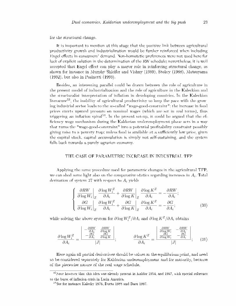
THE CASE OF PARAMETRIC INCREASE IN INDUSTRIAL TFP
Applying the same procedure used for parametric changes in the agricultural TFP,we can shed some light also on the comparative statics regarding increases in Ai. Totalderivation of system 27 with respect to Ai yields
∂RW
∂ logWi
∣∣∣∣Z
∂ logWZi
∂Ai+
∂RW
∂ logK
∣∣∣∣Z
∂ logKZ
∂Ai= −∂RW
∂Ai;
∂G
∂ logWi
∣∣∣∣Z
∂ logWZi
∂Ai+
∂G
∂ logK
∣∣∣∣Z
∂ logKZ
∂Ai= − ∂G
∂Ai; (30)
while solving the above system for ∂ logWZi /∂Ai and ∂ logKZ/∂Ai obtains
∂ logWZi
∂Ai=
∣∣∣∣∣ −∂RW∂Ai
∂RW∂ logK
− ∂G∂Ai
∂G∂ logK
∣∣∣∣∣|J |
;∂ logKZ
∂Ai=
∣∣∣∣∣ ∂RW∂ logWi
−∂RW∂Ai
∂G∂ logWi
− ∂G∂Ai
∣∣∣∣∣|J |
; (31)
Here again all partial derivatives should be values at the equilibrium point, and needto be considered separately for Kaldorian underemployment and for maturity, becauseof the piecewise nature of the real wage schedule.
53Note however that this idea was already present in Kaldor 1954, and 1967, with special reference
to the burst of in�ation crisis in Latin America.54See for instance Kalecky 1976, Dutta 1988 and Basu 1997.

24 Giovanni Valensisi
Following a conditional line of reasoning, let us suppose �rst that the equilibriumZ occurs during the Kaldorian underemployment phase; accordingly, the relevant ex-pressions for the partial derivatives should be computed from equations 18 and 23.After some algebra (shown with some more detail in Mathematical Appendix III.B)the above formulas reduce to
∂ logWZi
∂Ai= −γ + α(1− γ)(1− bLi)
βAi[γ + α(1− γ)]La1
|JKU |;∂ logKZ
∂Ai= −1− (1− γ)[1− α(1− b)]Li
βAi[γ + α(1− γ)]La1
|JKU |;
(32)which imply, under the assumed parametrization, that the derivatives ∂ logWZ
i /∂Aiand ∂ logKZ/∂Ai take the opposite sign of
∣∣JKU ∣∣. Like in the previous case, the corre-spondence principle ensures that
∣∣JKU ∣∣ is positive when Z is an unstable equilibrium,so that the direction in which the new equilibrium lies can be univocally determined.
To complete the conditional analysis, suppose instead that the equilibrium pointZ belongs to the maturity interval; in such case, the relevant partial derivatives inexpression 31 should be computed from equations 21 and 23. After some algebraicmanipulation this operation obtains:
∂ logWZi
∂Ai= − 1
β
1Ai
1|JMA|
;∂ logKZ
∂Ai= − 1
β
1Ai
1|JMA|
; (33)
in which JMA indicates the Jacobian corresponding to the maturity interval. Equation33 implies that the derivatives ∂ logWZ
i /∂Ai and ∂ logKZ/∂Ai take the opposite signof∣∣JMA
∣∣.In light of the correspondence principle, it can be shown (see Mathematical Ap-
pendix III.B) that ∣∣JMA∣∣ > 0 ⇒ µ > (1− β);
so that the sign of ∂ logWZi /∂Ai and ∂ logKZ/∂Ai can be univocally determined.
At this stage, it is therefore possible to summarize the comparative statics resultsas follows. A parametric increase in Ai
• shifts the unstable equilibrium (if any) towards the South-West, more preciselyit reduces the basin of attraction of the equilibrium of pure subsistence withzero capital stock; this statement holds in both Kaldorian underemployment andmaturity, since ∂ logWZ
i /∂Ai and ∂ logKZ/∂Ai are negative in both cases;
• moves the stable equilibrium (if any) towards north-east, increasing the steadystate level of capital and wages, since ∂ logWZ
i /∂Ai and ∂ logKZ/∂Ai in thiscase are both positive.
These results are illustrated graphically in �gure 4, which considers the case inwhich a poverty trap exists (dashed schedules represent the equilibrium loci beforethe productivity increase)55. The economic explanation goes as follows, regardless ofwhich phase the economy goes through. The increase in Ai raises, ceteris paribus, the
55In the absence of a poverty trap, the only impact of the industrial productivity increase would be
to increase the steady state level of capital and wages for the stable interception.

Dual economies, Kaldorian underemployment and the big push 25
Figure 4: The e�ect of an increase in industrial TFP
supply of manufactures, leading to a moderate increase in the agricultural terms oftrade and in agricultural wages, which in turn trigger an upwards adjustment of thenominal industrial wages. These factors explain the upwards move of the real wageschedule. The gains in terms of industrial productivity bring, however, a much largergain to entrepreneurs, boosting their pro�ts, and allowing a faster capital accumulation;this is re�ected in the upwards shift of the stationary capital locus. Since the verticalmovement of the K = 0 locus outweighs that of the real wage schedule56, the unstablelow-development equilibrium (if any) will occur for a lower level of capital stock (inthe �gure KZ > KZ′). Similarly to what happened for the agricultural TFP, technicalprogress in industry directly boosts the pro�tability of entrepreneurs, so that a self-sustaining accumulation of capital becomes viable even for lower capital stocks. Forexactly the same reasons, the equilibrium of full industrialization will always be pushedtowards higher levels of capital stock by improvements in industrial TFP, regardless ofthe phase of the economy.
VI. CONCLUSIONS
In line with our main objective, we have combined in this two-sector macro-modelseveral aspects emphasized by the neoclassical theory of growth and structural change,with other insights drawn from the more dated literature about dual economies andbig push. Interestingly, the adoption of an e�ciency wage mechanism in the urbanlabor market (unlike in the rural one), combined with technological external economies
56This can be veri�ed by directly computing ∂ logWi/∂ logAi for the real wage schedule and for the
stationary capital locus: this derivative in the latter case outweighs the correspondent derivative for
RW.

26 Giovanni Valensisi
in industry, are su�cient to rationalize a view of the agriculture industry shift à laKaldor, and to originate possible poverty traps that may justify policies of concertedinvestment to bring capital stock up to a minimum critical level.
Of course, Kaldor's structure of causality pivots around the central role of e�ectivedemand, while we retain a supply-driven framework, resembling rather closer Lewis'smodel of unlimited supply of labor. Nevertheless, the complex interactions betweenagriculture and industry, the importance of labor reallocation to the more dynamicsector, and the asymmetric working of the labor market represent common aspects thatlink the present work to the "Strategic factors in economic development", highlightingthe crucial role of industrialization and increasing returns in the process of development.
As concerns instead the long debate on the big push argument, the above analysishas shown how - in presence of a labor market characterized by the mismatch betweenthe wage and productivity levels in agriculture and industry - even moderate degreesof increasing returns in industry may be su�cient to give raise to poverty traps, sincethe e�ect of increasing returns if reinforced by the elastic supply of labor for the moredynamic industrial sector. While this result is encouraging for the plausibility of themechanisms outlined here, our model is surely very sensitive to the parametrizationadopted, and, likewise the majority of poverty trap models, it "tends to be lacking intestable quantitative implications"57. Nevertheless, we believe the mechanisms analyzedhere may well be relevant for LDCs, and above all of todays Sub-Saharan Africa, theregion with the closest conditions to our theoretical framework: extremely capital-pooragricultural sector, with widespread areas of subsistence agriculture.
Besides, this work has shown the peculiar relation between sectoral TFP, and thepossible bottlenecks to capital accumulation, explaining how increases in the TFP ofany of the two sectors, may help making the poverty trap if not less likely at leastless stringent. Interestingly, in the event of being stuck by a poverty traps, our modelsuggests two strategies, which also seem to be at the cornerstone of the Chinese eco-nomic success in the last twenty years: raising agricultural productivity and accumulat-ing physical capital, with special attention to the "social overhead capital". Now thatthese strategies are also becoming the pillar of Chinese growing economic interventionsin Sub-Saharan Africa, we may have the chance to see these policies at work in thoseeconomies with the closest resemblance to our conceptual set-up.
Mathematical Appendix
I. THE KALDORIAN UNDEREMPLOYMENT PHASE
A. DETERMINATION OF THE LABOR SUPPLY ELASTICITY
Substituting in the consumption expenditure �ow identity (equation 14), the valueof agricultural wages and rents (equations 5 and 6), and using the numeraire (equation
57The quotation is taken from Azariadis and Stachurski (2005), recognizing a limit which is common
to most models of poverty trap.

Dual economies, Kaldorian underemployment and the big push 27
15) and the fact that Π = β1−βWiLi; yields
P Xca +Xc
i = P Xsa +
1− sβ1− β
WiLi;
which combined with equation 13 obtains
Xci =
1− sβ1− β
WiLi;
Substituting Xci from the demand function (equation 1), using equations 8 and 5 to
express the agricultural terms of trade as a function of the nominal industrial wage, andapplying the labor market clearing relation and the food production function (equations11 and 3) yields
1− αα
1− β1− sβ
[(1− d)
1d
ω1d (1− b)γ
] 1γ+α(1−γ)
Aα(1−γ)
γ+α(1−γ)a (1− Li)
γ+α(1−γ)(1−b)γ+α(1−γ) = Wi
− (1−α)(1−γ)γ+α(1−γ) Li;
(34)Taking logs obtains
log
1− αα
1− β1− sβ
[(1− d)
1d
ω1d (1− b)γ
] 1γ+α(1−γ)
+α(1− γ)
γ + α(1− γ)logAa +
+(1− α)(1− γ)γ + α(1− γ)
logWi = −γ + α(1− γ)(1− b)γ + α(1− γ)
log [1− exp (logLi)] + logLi;
from which total di�erentiation yields the expression for the industrial labor supplyelasticity εLS mentioned in equation 17:
εLS =(1− α) (1− γ) (1− Li)γ + α(1− γ)(1− bLi)
;
B. DETERMINATION OF THE REAL WAGE SCHEDULE
To determine the real wage schedule, replace Li in equation 34 with its value from9, which obtains
Q Aα(1−γ)
γ+α(1−γ)a A
− 1β
i K−µ+β
β W
[1β
+(1−α)(1−γ)γ+α(1−γ)
]i =
=[1−A
1β
i (1− β)1β (E∗)
1−ββ W
− 1β
i Kµ+ββ
]− γ+α(1−γ)(1−b)γ+α(1−γ)
;
where Q is a constant de�ned as
Q =1− αα
(1− β)−1−ββ
1− sβ(E∗)−
1−ββ
[(1− d)
1d
ω1d (1− b)γ
] 1γ+α(1−γ)
.
Expressed in log terms, this equation is exactly the RW schedule mentioned in the text(equation 18).
C. THE EVOLUTION OF THE WAGE GAP

28 Giovanni Valensisi
Consider the expression for the agricultural wage relatively to the industrial one58
Wa
Wi=
(1− b)Aa (La)−b PaWi
;
using equations 8 and 5 to express Pa as a function of Wi, and then making use ofequation 11 and 9, the wage ratio can be rewritten as
Wa
Wi=
[(1− dω
) 1d
(1− b)α(1−γ)Aα(1−γ)a
] 1γ+α(1−γ)
W(1−α)(1−γ)γ+α(1−γ)i[
1−Ai1β (1− β)
1β (E∗)
1−ββ W
− 1β
i Kµ+ββ
]−bα(1−γ)γ+α(1−γ)
.
Taking logs, the wage ratio becomes
logWa
Wi=
1γ + α(1− γ)
log
[(1− dω
) 1d
(1− b)α(1−γ)Aα(1−γ)a
]+
(1− α)(1− γ)γ + α(1− γ)
logWi +
− bα(1− γ)γ + α(1− γ)
log[1−Ai
1β (1− β)
1β (E∗)
1−ββ exp
(µ+ β
βlogK − 1
βlogWi
)];
from which total di�erentiation, yields the following relation:
∂ log WaWi
∂ logK=
αb(µ+ β)(1− γ)LiβLa[γ + α(1− γ)]
+(1− γ)[β (1− α)La − αbLi]
βLa[γ + α(1− γ)]∂ logWi
∂ logK.
Substituting ∂ logWi
∂ logK in this expression with the coe�cient of the real wage scheduleobtained in equation 19, yields
∂ log WaWi
∂ logK=
(µ+ β)(1− γ)(1− α)[γ + α(1− γ)] + (1− γ)[β(1− α)La − αbLi]
> 0.
Since this derivative is strictly positive for the parametrization assumed above, the wageratio tends to grow along with increases in the capital stock, from values lower thanone (by construction) ultimately reaching one when the system enters the maturityphase and wage gap disappear. To see this, note that the logarithm is a monotonicallyincreasing transformation of the wage ratio and of the capital stock, hence the sign ofthe log-derivative ∂ log Wa
Wi/∂ logK equals the sign of the simple derivative of the wage
ratio to capital stock.
II. THE MATURITY PHASE
A. DETERMINATION OF THE LABOR SUPPLY ELASTICITY
As before, combining the consumption expenditure �ow identity (equation 14), withwage and rents determination and with food market clearing (equations 5, 12, 6 and13), and using the fact that Π = β
1−βWiLi; yields
Xci =
1− sβ1− β
Wi Li.
58The absolute wage gap is tied to the wage ratio by the following relation Wi−Wa = (1− WaWi
)Wi.
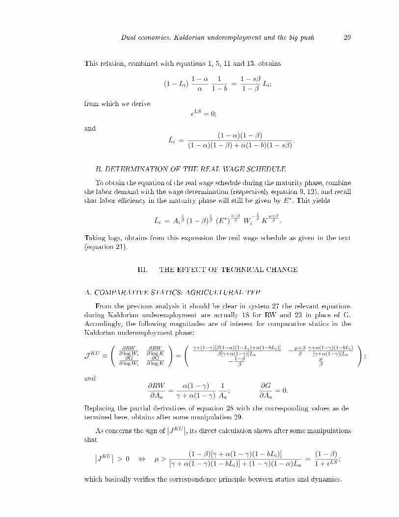
Dual economies, Kaldorian underemployment and the big push 29
This relation, combined with equations 1, 5, 11 and 13, obtains
(1− Li)1− αα
11− b
=1− sβ1− β
Li;
from which we derive
εLS = 0;
and
Li =(1− α)(1− β)
(1− α)(1− β) + α(1− b)(1− sβ).
B. DETERMINATION OF THE REAL WAGE SCHEDULE
To obtain the equation of the real wage schedule during the maturity phase, combinethe labor demand with the wage determination (respectively equation 9, 12), and recallthat labor e�ciency in the maturity phase will still be given by E∗. This yields
Li = Ai1β (1− β)
1β (E∗)
1−ββ W
− 1β
i Kµ+ββ .
Taking logs, obtains from this expression the real wage schedule as given in the text(equation 21).
III. THE EFFECT OF TECHNICAL CHANGE
A. COMPARATIVE STATICS: AGRICULTURAL TFP
From the previous analysis it should be clear in system 27 the relevant equationsduring Kaldorian underemployment are actually 18 for RW and 23 in place of G.Accordingly, the following magnitudes are of interest for comparative statics in theKaldorian underemployment phase:
JKU ≡
(∂RW∂ logWi
∂RW∂ logK
∂G∂ logWi
∂G∂ logK
)=
(γ+(1−γ)[β(1−α)(1−Li)+α(1−bLi)]
β[γ+α(1−γ)]La −µ+ββ
γ+α(1−γ)(1−bLi)[γ+α(1−γ)]La
−1−ββ
µβ
);
and∂RW
∂Aa=
α(1− γ)γ + α(1− γ)
1Aa
;∂G
∂Aa= 0.
Replacing the partial derivatives of equation 28 with the corresponding values as de-termined here, obtains after some manipulation 29.
As concerns the sign of∣∣JKU ∣∣, its direct calculation shows after some manipulations
that∣∣JKU ∣∣ > 0 ⇔ µ >(1− β)[γ + α(1− γ)(1− bLi)]
[γ + α(1− γ)(1− bLi)] + (1− γ)(1− α)La=
(1− β)1 + εLS
;
which basically veri�es the correspondence principle between statics and dynamics.

30 Giovanni Valensisi
During maturity, instead, the relevant equations for system 27 are equation 21 (forRW) and 23 for G. Accordingly, we have
JMA ≡
(∂RW∂ logWi
∂RW∂ logK
∂G∂ logWi
∂G∂ logK
)=
(1
βLa− µ∗ββLa
−1−ββ
µβ
).
and∂RW
∂Aa= 0;
∂G
∂Aa= 0.
Finally replacing the partial derivatives in equation 28 with the corresponding valuesdetermined here for the maturity phase, directly obtains
∂ logWZi
∂Aa= 0;
∂ logKZ
∂Aa= 0;
proving that the equilibrium occurring in the maturity phase (if any) is invariant toparametric changes in Aa, regardless of its stability properties.
B. COMPARATIVE STATICS: INDUSTRIAL TFP
Starting with Kaldorian underemployment, the relevant equations for system 30are 18 (for RW), and 23 (for G). Hence, in addition to the matrix JKU de�ned above,the magnitudes of interest for the comparative statics regarding Ai in the Kaldorianunderemployment phase are:
∂RW
∂Ai= −γ + α(1− γ)(1− bLi)
β[γ + α(1− γ)]La1Ai
;∂G
∂Ai=
1β
1Ai
;
Replacing these values for the corresponding partial derivatives in equation 31, obtainsafter some manipulation 32. Recalling �nally the condition for a positive determinantof JKU , yields the comparative statics result mentioned in the text.
As concerns the maturity phase, instead, the relevant Jacobian
JMA ≡
(∂RW∂ logWi
∂RW∂ logK
∂G∂ logWi
∂G∂ logK
)=
(1
βLa− µ∗ββLa
−1−ββ
µβ
);
can be derived directly from equations 21 (for RW) and 23 for G. From these sameequation, it is possible to compute the magnitudes
∂RW
∂Ai= − 1
β
1Ai
;∂G
∂Ai=
1β
1Ai.
Substituting these expressions in equation 31 obtains after a bit of algebra equation 33.
Finally, the direct calculation of∣∣JMA
∣∣ veri�es the correspondence principle, estab-lishing precisely that ∣∣JMA
∣∣ > 0 ⇔ µ > (1− β);
and with this last condition the sign of the derivatives ∂ logWZi /∂Ai and ∂ logKZ/∂Ai
can be univocally determined.

Dual economies, Kaldorian underemployment and the big push 31
References
[1] Aghion, P., and Bolton, P. A theory of trickle-down growth and development.Review of Economic Studies 64 (1997), 151�172.
[2] Akerlof, G. Labor contracts as partial gift exchange. Quarterly Journal of
Economics 97 (1982), 543�569.
[3] Akerlof, G., and Yellen, J. E�ciency wage models of the labor market.Cambridge University Press, 1986.
[4] Arrow, K. The economic implications of learning by doing. Review of Economic
Studies 29 (1962), 155�173.
[5] Azariadis, C. The theory of poverty traps: what have we learned? (in "PovertyTraps") Bowles, Durlauf and Ho� (editors) Princeton University Press, 2005.
[6] Azariadis, C., and Drazen, A. Threshold externalities in economic develop-ment. The Quarterly Journal of Economics 105 (1990), 501�526.
[7] Azariadis, C., and J., S. Poverty traps. (in "Handbook of economic growth")Aghion and Durlauf (editors) Elsevier Science Publishers, 2005.
[8] Banerjee, A., and Newman, A. Occupational choice and the process of devel-opment. Journal of Political Economy 101 (1993), 274�298.
[9] Barro, R. Economic growth in a cross section of countries. The Quarterly Journalof Economics 106 (1991), 407�443.
[10] Barro, R., and Sala-i Martin, X. Economics growth. McGraw-Hill, 1995.
[11] Basu, K. Analytical Development Economics: The Less Developed Economy Re-
visited. MIT press, 1997.
[12] Bhaduri, A. Alternative development strategies and the rural sector. (in "Eco-nomic crisis and the Third World agriculture") Singh and Tabatabai (editors)Cambridge University Press, 1993.
[13] Bhaduri, A. Structural change and economic development: on the relative roles
of e�ective demand and the price mechanism in a dual economy. (in "Rethinkingdevelopment economics") Ha Joon Chang (editor) Anthem Press, 2003.
[14] Bowles, S. The production process in a competitive economy: Walrasian, neo-hobbesian and marxian models. American Economic Review 75 (1985), 16�36.
[15] Chenery, H., and Syrquin, M. Patterns of development, 1950-1970. OxfordUniversity Press, 1975.
[16] Dixit, A. Models of dual economies. (in "Models of economic growth") Mirleesand Stern (editors) Macmillan, 1989.
[17] Dutta, J. The wage good constraint on a developing economy: Theory andevidence. Journal of Development Economics 28 (1988), 341�363.

32 Giovanni Valensisi
[18] Easterly, W. Reliving in the 50s: the big push, poverty traps, and takeo�s ineconomic development. mimeo (2006).
[19] Fei, J., and Ranis, G. A theory of economic development. American Economic
Review 51 (1961), 533�565.
[20] Galor, O. Convergence? inferences from theoretical models. The Economic
Journal 106 (1996), 1056�1069.
[21] Galor, O., and Zeira, J. Income distribution and macroeconomics. Review of
Economic Studies 60 (1993), 35�52.
[22] Gandolfo, G. Economic dynamics. Springer, 1997.
[23] Hansen, G., and Prescott, E. Malthus to Solow. American Economy Review
92 (2002), 1205�1217.
[24] Jorgenson, D. The development of a dual economy. Economic Journal 71
(1961), 309�334.
[25] Kaldor, N. Strategic Factors in Economic Development. Ithaca: Cornell Univer-sity, 1967.
[26] Kaldor, N. Productivity and growth in manufacturing industry: a reply. Eco-
nomica 35 (1968), 385�391.
[27] Kraay, A., and Raddatz, C. Poverty traps, aid, and growh. Journal of Devel-opment Economics 82 (2007), 315�347.
[28] Kremer, M. The o-ring theory of economic development. Quarterly Journal of
Economics 108 (1993), 551�575.
[29] Krugman, P. The narrow moving band, the dutch disease, and the competitiveconsequences of mrs. thatcher. Journal of Development Economics 27 (1987),41�55.
[30] Krugman, P. Toward a counter-counterrevolution in development theory. Pro-
ceedings of the Annual World Bank Conference 1992 (World Bank Economic Re-
view) (1992).
[31] Kuznets, S. Modern economic growth. Yale University Press, 1966.
[32] Lewis, A. Economic development with unlimited supplies of labor. Manchester
School of Economics and Social Studies 28 (1954), 139�191.
[33] Lewis, A. Unlimited labor: further notes. Manchester School of Economics and
Social Studies 32 (1958), 1�32.
[34] Mankiw, G., Romer, D., and Weil, D. A contribution to the empirics ofeconomic growth. The Quarterly Journal of Economics 107 (1992), 407�437.
[35] Matsuyama, K. Agricultural productivity, comparative advantage, and economicgrowth. Journal of Economic Theory 58 (1992), 317�334.

Dual economies, Kaldorian underemployment and the big push 33
[36] Murphy, K., Shleifer, A., and Vishny, R. Income distribution, market sizeand industrialization. Quarterly Journal of Economics 104 (1989), 537�564.
[37] Murphy, K., Shleifer, A., and Vishny, R. Why is rent-seeking so costly togrowth? American Economic Review 83 (1993), 409�414.
[38] Nelson, R. A theory of the low level equilibrium trap in underdevelopedeconomies. American Economic Review 46 (1956), 894�908.
[39] Nurkse, R. Problems of Capital Formation in Underdeveloped Countries. Oxford:Basil Blackwell, 1953.
[40] Pasinetti, L. Structural Economic Dynamics. Cambridge University Press, 1993.
[41] Preobrazhensky, E. The new economics. Oxford University Press, 1965.
[42] Quah, D. Galton's fallacy and tests of the convergence hypothesis. The Scandi-
navian Journal of Economics 95 (1993), 427�443.
[43] Quah, D. Twin peaks: growth and convergence in models of distribution dynam-ics. The Economic Journal 106 (1996), 1045�1055.
[44] Ray, D. Development economics. Princeton University Press, 1998.
[45] Ros, J. Development theory and the economics of growth. The University ofMichigan Press, 2000.
[46] Ros, J., and Skott, P. The big push in an open economy with non-tradableinputs. Journal of Post Keynesian Economics 20 (1997), 149�162.
[47] Rosenstein-Rodan, P. Problems of industrialization in Eastern and South-Eastern Europe. Economic Journal 53 (1943), 202�211.
[48] Rosenzweig, M. R. Labor Markets in Low Income Countries. (in "Handbookof development economics") Chenery and Srinivasan (editors) Elsevier SciencePublishers, 1988.
[49] Sachs, J. The end of poverty: how we can make it happen in our lifetime. PenguinBooks, 2005.
[50] Sala-i Martin, X. The classical approach to convergence analysis. The EconomicJournal 106 (1996), 1019�1036.
[51] Scitovsky, T. Two concepts of external economy. Journal of Political Economy62 (1954), 143�151.
[52] Smith, A. Early draft of part of the Wealth of Nations. (in "Lectures of Jurispru-dence") Meek, Raphael and Stein (editors) Claredon Press, 1978.
[53] Solow, R. M. A contribution to the theory of economic growth. Quarterly
Journal of Economics 70 (1956), 65�94.
[54] Solow, R. M. Technical change and the aggregate productio function. The
Review of Economics and Statistics 39 (1957), 312�320.

34 Giovanni Valensisi
[55] Solow, R. M. Perspectives on growth theory. Journal of Economic Perspectives8 (1994), 45�54.
[56] Stiglitz, J. Comment on toward a counter-counterrevolution in developmenttheory. Proceedings of the Annual World Bank Conference 1992 (World Bank
Economic Review) (1992).
[57] Stokey, N. Learning by doing and the introduction of new goods. Journal of
Political Economy 96 (1988), 701�717.
[58] Syrquin, M. Sector proportions and Economic Development: the evidence since
1950. (in "The balance between agriculture and industry in economic develop-ment") Panchamukhi and Williamson(editors) Macmillan, 1989.
[59] Taylor, L. Theories of Sectoral Balances. (in "The balance between agricultureand industry in economic development") Panchamukhi and Williamson(editors)Macmillan, 1989.
[60] Verdoorn, P. J. Fattori che regolano lo sviluppo della produttività del lavoro.L'industria 1 (1949), 45�53.
[61] Young, A. Increasing returns and economic progress. Economic Journal 38
(1928), 527�542.