durham e-theses stability and wave motion problems in
TRANSCRIPT

Durham E-Theses
Stability and wave motion problems in continuous
media with second sound
Jaisaardsuetrong, Jiratchaya
How to cite:
Jaisaardsuetrong, Jiratchaya (2009) Stability and wave motion problems in continuous media with second
sound, Durham theses, Durham University. Available at Durham E-Theses Online:http://etheses.dur.ac.uk/2121/
Use policy
The full-text may be used and/or reproduced, and given to third parties in any format or medium, without prior permission orcharge, for personal research or study, educational, or not-for-pro�t purposes provided that:
• a full bibliographic reference is made to the original source
• a link is made to the metadata record in Durham E-Theses
• the full-text is not changed in any way
The full-text must not be sold in any format or medium without the formal permission of the copyright holders.
Please consult the full Durham E-Theses policy for further details.

Academic Support O�ce, Durham University, University O�ce, Old Elvet, Durham DH1 3HPe-mail: [email protected] Tel: +44 0191 334 6107
http://etheses.dur.ac.uk
2
stability and Wave Motion Problems in Continuous Media
with Second Sound
Jiratchaya Jaisaardsuetrong
The copyright of this thesis rests with the author or the university to which it was submitted. No quotation from it, or Information derived from it may be published without the prior written consent of the author or university, and any information derived from it should be acknowledged.
A Thesis presented for the degree of Doctor of Philosophy
Numerical Analysis Department of Mathematical Sciences
University of Durham England
July 2009
2 9 SEP 2009

Dedicated to M y family

Stability and Wave Motion Problems in Continuous Media with Second Sound
Jiratchaya Jaisaardsuetrong
Submitted for the degree of Doctor of Philosophy
July 2009
Abstract
I n this thesis we investigate thermal convection and wave motion in models of second
sound such as the Cattaneo model, Green and Laws model, Batra model, and Green
and Naghdi model. For the Green and Laws and Batra models we also investigate
questions of stability and uniqueness.
The term second sound means the transport of heat as a thermal wave. The
models are all presented wi th in the framework of continuum mechanics. We use a
mathematical technique involving an acceleration wave to solve some problems. Fur
thermore, i n one of the chapters we use a numerical method, namely a D"^ Chebyshev
tau method to f ind eigenvalues of a thermal convection problem. This technique is
a highly accurate method.
In Chapter two we study thermal convection w i t h the Cattaneo model. The
model is about thermal convection in a layer of f lu id heated f r o m below. We also
employ Chebyshev tau method to obtain numerical results for the model.
In Chapter three we study various properties such as instabili ty and uniqueness
of the model of second sound which is derived by Green and Laws. We investigate
the model of Green and Laws for which the generalized temperature (j) depends on 6
and 6. We also show differences between the results when the boundary and in i t ia l
conditions have been changed.
In Chapter four we study uniqueness, instability and wave motion of a Batra
model. I n Chapter five we investigate thermal waves i n a r igid heat conductor. This
is a more recent model of heat transport in a r igid body, namely that derived by
I V
Green and Naghdi.
In the final chapter, Chapter six, we consider a generahzation of the theory of
Chapter five, to include fluid mechanical behaviour. We adopt a special relation for
the Helmholtz free energy in the model of Green and Naghdi. We analyse behaviour
of an acceleration wave for the model.

Declaration
The work in this thesis is based on research carried out in the Numerical Analysis
Group, the Department of Mathematical Sciences, University of Durham, England.
No part of this thesis has been submitted elsewhere for any other degree or quali
fication and i t is all my own work w i t h the exception of Chapter 5. Chapter 5 was
wr i t ten in collaboration wi th Prof. Brian Straughan of the University of Durham,
England. The content of Chapter 5 is published in [81
Copyright (c) 2009 by Jiratchaya Jaisaardsuetrong.
"The copyright of this thesis rests w i t h the author. No quotations f rom i t should be
published without the author's prior wri t ten consent and information derived f rom
i t should be acknowledged".

Acknowledgements
I would like to thank my supervisor Prof. Brian Straughan w i t h my deepest grat
itude and respect. His guidance, encouragement and patience have allowed me to
complete this work.
Thanks also to Dr. James Blowey for his kindness f rom the first day I arrived
in Durham and throughout my stay. Also, thanks to Dr. Alan Craig and Dr. John
Coleman who have schooled me in aspects of mathematics. In addition, thanks to
Dr. Max Jensen, Dr. Djoko Wirosoetisno and Dr Miguel Moyers-Gonzalez who
have inspired my mathematics. Thanks to Dr. M Imran for preparing L A T E X
template which have helped myself and many postgraduates in the mathematical
science department save much of our time.
Thanks to my colleagues in the Numerical Analysis group, Statistics and Prob
abili ty group, and Pure Mathematics group for their friendships. Thanks to my
friend. Dr. Pisuttawan Sripirom, for her friendship and L A T E X guidance. I also
thank everyone in Department of Mathematical Sciences at University of Durham
for their assistance, especially Ms. Fiona Gibl in for her administrative work in
managing my application to study here.
I extend my wholehearted thanks to my father, mother and my sisters for their
love and support. Also, thank to my Tha i friends in Durham and my colleagues in
Ubonratchathani University for their lovely friendships.
Finally, I would like to thank the Royal Thai Government for the scholarship
throughout my study at the University of Durham.
V I
Contents
Abstract iii
Declaration v
Acknowledgements vi
1 Introduction 1
1.1 Cattaneo theory 3
1.2 Outline of thesis 8
2 Thermal convection with the Cattaneo model 10
2.1 D"^ Chebyshev tau method 10
2.2 Hydrodynamic stability eigenvalue problems 13
2.3 Chebyshev tau method, Orr-Sommerfeld equation 14
2.4 Thermal convection wi th the Cattaneo law 16
2.5 Numerical results 21
3 Green and Laws model 23
3.1 Derivation of the model 23
3.2 Uniqueness for the Green and Laws model wi th ki constant 26
3.3 Uniqueness for Green and Laws model w i t h ki = ki{x) 29
3.4 Continuous dependence of the thermal energy 30
3.5 Uniqueness and continuous dependence for a related model 32
3.6 A n instability result for a solution to (3.13) 35
3.7 Uniqueness on an unbounded spatial domain 37
3.8 A non-standard problem for equation (3.13) 41
v i i

Contents vm
4 Batra Model 47
4.1 Model and uniqueness? 47
4.2 Exponential growth 51
4.3 Explosive instability in a Batra model 55
4.4 Thermal discontinuity waves in the Batra theory 61
5 Thermal waves in a rigid heat conductor 65
5.1 Basic equations and thermodynamic restrictions 67
5.2 Acceleration waves 69
5.3 Homogeneous region 72
5.4 AmpHtude behaviour 73
6 Green-Naghdi theory for a fluid. 84
6.1 Conclusions 88

List of Figures
2.1 Diagram il lustrating fluid heated f rom below 17
3.1 Diagram il lustrat ing unbounded spatial domain 37
I X

List of Tables
2.1 Cri t ical Rayleigh numbers 21

Chapter 1
Introduction
I n this thesis we study several models for "second sound". The term second sound
refers to the transport of heat as a thermal wave. I n particular, we study mod
els for second sound which have been derived using the principles of continuum
thermodynamics. A lucid introduction to continuum mechanics may be found in
pages 310-344 of the book by Fabrizio [46]. The mathematical techniques we use
are based primari ly on two ideas. The first is to analyse problems of linear instabil
i ty in a hydrodynamics setting. This involves solving eigenvalue problems numeri
cally and to this end we employ a D^-Chebyshev tau method. The Chebyshev tau
method is a highly accurate numerical method, which is described in Chapter 2.
This technique has been very successful in yielding sharp results for hydrodynamic
stability problems and suitable (mainly recent) references are Carr [17,18], Chang
et al. [23], Dongarra et al. [41], H i l l [70,71], H i l l & Straughan [72-74], Orszag [125],
Straughan [168-170], Straughan & Walker [174-176], Webber [188,189 .
The second mathematical technique we employ is that of acceleration waves. This
technique has been in employment for some time, see Chen [24], Fabrizio and Morro
49], Ogden [124], Truesdell and Toupin [181], TVuesdell and NoU [180]. However,
i t is s t i l l a very powerful technique which is much in current use. This is because
i t yields a means of analysing a fu l ly nonlinear problem w i t h no approximation
and then yields valuable results which allow one to test the validity of the physical
theory. To indicate just how important this technique is in the recent literature we
list the following references, all of which deal w i t h acceleration waves, or very similar
1
Chapter 1. Introduction
analyses such as these involving other discontinuity waves, Chen [24], Christov et
al. [27,28], Ciarletta & lesan [30], Ciarletta & Straughan [31-33], Ciarletta et al.
34], Curro et al. [39], Eremeyev [45], Fabrizio & Morro [49], Fu & Scott [53-55],
Gultop [66], lesan k Scalia [80], Jordan [83-88], Jordan & Christov [89], Jordan
and Feuillade [90], Jordan & Puri [91,92], Jordan & Straughan [95], Kameyama &
Sugiyama [100], L in & Szeri [103], Mariano & Sabatini [112], Marasco [110], Marasco
& Romano [111], Mentrell i et al. [114], Ogden [124], Ostoja-Starzewski k Trebicki
[126], Rai [156], Rajagopal & Truesdell [157], Ruggeri k Sugiyama [160], Sabatini
k Augusti [161], Straughan [170,172], Sugiyama [179], Truesdell k Toupin [181],
Truesdell k Nol l [180], Valenti et aJ. [186], Weingartner et al. [190,191], Whi tham
192 .
The topic of second sound is a very hot one in the current applied mathematical
literature. There are many theories for heat propagation as a wave in r igid bodies,
in fluids, in gases, in elastic bodies, and even in materials w i t h much more exotic
structure. A thorough review of second sound theories, generalised heat conduction
theories, and acceleration waves is contained in the book by Straughan [170] and
in the forthcoming book by Straughan [171]. The material for this introduction
and the cited references are taken f rom the books of Straughan [170,171]. To give
an idea of the extent of interest we quote the following references, all of which are
dealing wi th some aspect of second sound, Alvarez et al. [1], Alvarez et al. [2], Anile
k Romano [6], Bargman k Steinmann [8-10], Bargmann et al. [11], Bargmann
et al. [7], Brusov et al. [14], Buishvih et al. [15], Cai et al. [16], Cattaneo [19],
Caviglia et al. [20], Chandrasekhariah [21,22], Chen k Gur t in [25], Christov k
Jordan [26], Cimmelli k Prischmuth [35], Ciancio k Quintanilla [29], Coleman et
al. [36,37], Coleman k Newman [38], De Cicco k Diaco [40], Dreyer k Struchtrup
43], Duhamel [44], Fabrizio et ai. [48], Fabrizio et al. [47], Fichera [50], Franchi k
Straughan [52], Green [57], Green k Laws [58], Green k Naghdi [60-65], Gur t in k
Pipkin [67], Han et al. [68], Hetnarski k Ignaczak [69], Horgan k Quintanilla [75],
lesan [76-78], lesan k Nappa [79], Jaisaardsuetrong k Straughan [81], Johnson et al.
82], Jordan k Puri [94], Joseph k Preziosi [96,97], Jou et al. [98], Jou k Criado [99],
Kaminski [101], Lindsay k Straughan [105,106], L in k Payne [102], Linton-Johnson

1.1. Cattaneo theory
et al. [107], Loh et al. [108], Metzler & Compte [115], Meyer [116], M i t r a et al. [117],
Morro et al. [118], Morro & Ruggeri [119,120], Payne & Song [130-136], Puri k
Jordan [137-140], Puri & Kythe [141, 142], Quintanilla [143-145], Quintanilla k
Racke [146-149], Quintanil la & Straughan [150-155], Roy et al. [158], Ruggeri [159],
Saleh & A l - N i m r [162], Sanderson et al [163], Serdyukov [164], Serdyukov et al. [165],
Shnaid [166], Straughan [169-171], Straughan & Pranchi [173], Su et al. [178], Su &
Dai [177], Tzou [182,183], Vadasz [185], Vadasz et al. [184], Vedavarz et al. [187],
Zhang & Zuazua [193 .
1.1 Cattaneo theory
To give a precise application of acceleration wave analysis we begin w i t h an example
of heat propagation in a r igid solid. Straughan [170], pp. 349-360 describes these
ideas in a porous medium when the heat flux laws are of Cattaneo type and then of
dual phase lag type. We follow the presentation given there. The basic equations are
those of an energy balance, and a constitutive equation for the heat flux q. Thus, let
e be the internal energy of the body per unit mass and let 0{x, t) be the temperature.
For simplicity, we here restrict attention to one space dimension and so ^ = 0{x,t),
where wave propagation wi l l be in the x-direction. The energy balance law is in
three-dimensions ds dqi
or
pi = (1.2)
Throughout, standard indicial notation is employed w i t h a repeated index denoting
summation over 1,2 or 1,2,3.
In the one-dimensional case (1.1) becomes
The general theory of acceleration waves and shock waves in nonlinear elastody-
namics is covered in detail in Chen [24] and in Fabrizio k Morro [49], pages 518-532
for acceleration waves and pages 532-541 for shock waves. Truesdell k. Toupin [181

1.1. Cattaneo theory
and Truesdell & Noll [180] cover many aspects of acceleration waves and singular
surfaces, in general.
To illustrate the basic concepts of acceleration wave analysis, we mostly restrict
attention to a plane acceleration wave moving in the direction of the x—axis, wi th
one-dimensional motion. The precise definition of an acceleration wave depends
on the material comprising the body we are examining. However, i t wi l l involve a
surface iS across which certain derivatives of the functions defining the problem wi l l
have discontinuities. A precise definit ion of an acceleration wave w i l l be given in the
context in which i t occurs.
For a funct ion h{x, t) we define
h'^{x,t) = lim h{x,t) f rom the right, x—^S
h {x,t) = l i m h{x,t) f rom the left.
In particular, /i+ is the value of / i at 5 approaching f rom the region which S is about
to enter. The jump of h at 5, wr i t t en as [h], is,
[h] = h--h+. (1.4)
A key relation in acceleration wave analysis (or generally in any discontinu
i ty analysis) is the kinematic condition of compatibihty, sometimes known as the
Hadamard relation, 6^ 6t
where S/6t denotes the t ime derivative at the wave. (The Hadamard relation is
discussed in detail in Chen [24], Appendix 1, and also in Truesdell & Toupin [181],
Section 180.)
From the definition of [h] we may prove the relation for the j ump of a product
of functions g, h,
gh] = g+ [h] + [g] + [g][h]. (1.6)
We use this relation extensively throughout this thesis when calculating the wave
amplitudes.

1.1. Cattaneo theory
When K = K{6) and e = e{0), equation (1.3) together w i t h the Cattaneo law,
Cattaneo [19], present us w i t h the system of equations
Tqt + q = -K{e)9,
pseOt = -Qx, (1.7)
where r is a relaxation time.
Let us define an acceleration wave S for system (1.7) to be a surface across
which 9t,9x,(}t, Qx their higher derivatives suffer a finite discontinuity, jump, but
6, q e C ° ( R X (0,oo)). Then taking the j ump of (1.7) we see that
(1.8)
r[q^] = -K[dx]
pee[9t] = -[QX]-
To progress beyond (1.8) we use the Hadamard relation to find
[Qi] = -V[QX], [Ot] = -V[9xi
and then (1.8) become
-rVlqx] = -K[9x],
-peeV[9x] = - [qx],
or, wr i t ing in matr ix form,
-TV ^ \ ( [ x] 1 -psev) \ [9x]
For a non-zero solution of this we require
-TV K
1 -peeV
and so
V 2 K{e+) pTeg{9+y
where 9'^ denotes the temperature immediately ahead of the wave.
(1.9)
(1.10)

1.1. Cattaneo theory
Equation (1.10) shows that in the r igid body a temperature wave moves to the
right while an equivalent wave moves to the left w i th speed V, where
We may analyse the solution behaviour at the wave in much greater detail than
this. To do this define the wave amphtudes a and b by
a{t) = [9,], b{t) = [q,] (1.12)
and then differentiate each of (1.7) w i th respect to x,
peeedtOx + pseOtx = -Qxx, (1-13)
where K' = dK/dO.
To simplify the analysis we suppose the region ahead of the wave is in thermal
equilibrium, i.e. 9= constant.
This means
9^ = constant, 9+ = 9^ = 0. (1.14)
We take the jumps of (1.13) and use the product relation (1.6), recalling (1.14) to
deduce
r[qtx] + [QX] = -K'[9^]^ - K%^\
psee[9t][9x]+pee[etx\ = -[Qa:x]- (1.15)
Next, we use the Hadamard relation to see that
f = M + V 1 , „ 1 , | = l»j + y l« j
and employ these expressions in (1.15). In this manner one finds
P^e{jl - y%x]^ - peeeVa'' = -[9 ] (1.16)

1.1. Cat taneo theory
Prom (1.9) we know that
rVb = Ka, or b = —TJCL. TV
Using this we may deduce a satisfies the equations (note V is constant since 9'^ —
constant)
pee^ - peeV[9^x] - peeeVa^ = - [ f c ] (1-17)
Divid ing by K/V, where K/V y^O these yield
5a T V \ , 1 K'V 2 ,,rz, 1
| - m x ] - ^ V a ^ = - - M . (1.18) ot £e pee
Now, add both equations to find
2— - 9xx -[p + - ° + " F - ~ \ / a ' = 0. (1.19 5t \ K pee J r \K EQ )
Thanks to the wavespeed relation (1.10), the coefficient of [^x^] is zero. This yields
the following equation for the wave amplitude a,
where the constant Q is given by
1 / / T V _ eeeV\ ^~ 2 \ K Be J
= 1 / K{e+) fKe{9+) _ eee{n\ 2y frree{9+)\K{e+) £ e ( ^ + ) / ^ ' ^
To solve (1.20) we put u= l/a and then find
Using the integrating factor
5t 2T ^
^ ( e - / ^ - ^ ) = Ce- /^^
1.2. Out l ine of thesis
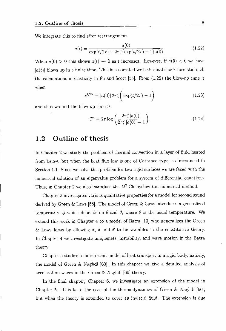
We integrate this to f ind after rearrangement
exp (V2r ) + 2 r C { e x p ( V 2 r ) - l } a ( 0 ) ' ^ " '
When a(0) > 0 this shows a{t) —> 0 as i increases. However, i f a(0) < 0 we have
|a(t)l blows up in a f ini te time. This is associated w i t h thermal shock formation, cf.
the calculations in elasticity in Fu and Scott [55]. Prom (1-22) the blow-up t ime is
when
e'/2^ = |a(0)| 2TC exp(^/2T) - 1 (1.23) \ y
and thus we f ind the blow-up t ime is
T* = 2 r l o g f - M m ^ y (1.24)
1.2 Outline of thesis
I n Chapter 2 we study the problem of thermal convection in a layer of f lu id heated
f rom below, but when the heat f lux law is one of Cattaneo type, as introduced in
Section 1.1. Since we solve this problem for two r igid surfaces we are faced wi th the
numerical solution of an eigenvalue problem for a system of differential equations.
Thus, in Chapter 2 we also introduce the D'^ Chebyshev tau numerical method.
Chapter 3 investigates various qualitative properties for a model for second sound
derived by Green & Laws [58]. The model of Green & Laws introduces a generalized
temperature 0 which depends on 6 and 9, where 9 is the usual temperature. We
extend this work in Chapter 4 to a model of Batra [13] who generalizes the Green
& Laws ideas by allowing 9, 9 and 9 to be variables in the constitutive theory.
In Chapter 4 we investigate uniqueness, instability, and wave motion in the Batra
theory.
Chapter 5 studies a more recent model of heat transport in a rigid body, namely,
the model of Green & Naghdi [60]. I n this chapter we give a detailed analysis of
acceleration waves in the Green & Naghdi [60] theory.
I n the final chapter. Chapter 6, we investigate an extension of the model in
Chapter 5. This is to the case of the thermodynamics of Green & Naghdi [60],
but when the theory is extended to cover an inviscid fluid. The extension is due

1.2. Out l ine of thesis
to Quintanilla k. Straughan [155]. We consider a different constitutive tfieory f rom
Quintanil la & Straughan [155], and study the development of an acceleration wave.
Chapter 2
Thermal convection with the
Cattaneo model
Our goal in this section is to solve a thermal convection problem. Firstly, we intro
duce a numerical method.
2.1 D'^ Chebyshev tau method
To describe the Chebyshev tau technique we follow Dongarra et al. [41] and consider
a simple example. Consider the equation and boundary conditions,
Lu=u" + Xu = ^, x e ( - l , l ) ,
u ( - l ) = « ( l ) = 0, (2.1)
where the differential operator L is defined as indicated.
Now write l i as a f ini te series of Chebyshev polynomials
N+2
= ^ t t f e T f c ( x ) . (2.2) fc=0
The idea is that (2.2) represent truncations of an infinite series. Due to the trun
cation, the tau method argues that rather than solving (2.1) one instead solves the
equation
Lu = TiTyv+i + T2TM+2 (2.3)
10

2.1. C h e b y s h e v t a u method 11
where T I , T2 are tau coefficients which may be used to measure the error associated wi th the truncation of (2.1).
To reduce (2.1) to a finite-dimensional problem the inner product w i th % is taken
of (2.3) in the weighted L ^ ( - l , 1) space wi th inner product
and associated norm ||-||. The Chebyshev polynomials are orthogonal in this space,
and then f rom (2.3) we obtain (A^ + 1) equations
{Lu,Ti) = 0 i = 0,l,...,N. (2.4)
There are two further conditions which arise f rom (2.3),
( L u , r ^ + , ) = r , | |T ;v+; | | ' , ; = 1,2,
and these may effectively be used to calculate the r 's . The two remaining conditions
are found f rom the boundary conditions, which since r „ ( ± l ) = ( ± 1 ) " , yield
^ ( - l ) " w „ = 0, 5 ] ^ „ = 0. (2.5) n=0 n=0
Equations (2.4) and (2.5) yield a linear system of (A^ + 3) equations for the (A'' + 3)
unknowns Ui, i — 0,..., N + 2.
The derivative of a Chebyshev polynomial is a Hnear combination of lower order
Chebyshev polynomials, in fact
n - l
Tn' = 2 n ^ T k , neven, fc=i n-l
Tn' = 2n^Tk + nTo, n odd. (2.6)
Then (2.4) becomes
w f ) + Aui = 0, 2 - 0 , . . . , i V , (2.7)
where the coefficients ^ are given by
p=N+2
Ci
p=N+2
p=i+2 p+i even

2.1. C h e b y s h e v tau method 12
w i t h the numbers Ci being defined by CQ = 2, Cj = 1, i = 1, 2 , . . . . (Actually, (2.8) is really a truncation to the A'' - I - 2th polynomial of an infini te expansion.) Equations (2.7) and (2.5) represent a matr ix equation
Ax = -XBx, (2.9)
w i t h X = ( u o , . . . , UN+2Y• However, the B matr ix is inevitably singular due to the
way the boundary condition rows are added to A. Indeed, the last two lines of B
are composed of zeros, while the upper left ( A - I - 1) x ( A - I - 1) part is simply the
identity.
To clarify this point, we observe
N+2
5=0 yv+2 ,N+2
s=0 ^r=0 N+2 ,N+2 V
r=0 ^s=0 /
and so we may make the identification
^ + 2
Similarly,
and, therefore.
s=0
N + 2 . N + 2 V
7^^ Kl^^ /
u.
r=0 ^ s=0
N + 2
s=0
N+2 N+2
= Y Dr,s Y ^s,kUk
s=0 k=0
N+2 N+2
= ^ ^ Dr,sDs,kUk • s=0 k=Q
This allows us to introduce the diiTerentiation matr ix D, and second differentiation

2.2. H y d r o d y n a m i c stabiHty eigenvalue problems. 13
matrix which are shown to have components
Do,2j-i = 2; - 1, > 1,
A , i + 2 , - i = 2{i + 2j - 1), i> I, J > 1,
Dl2j = \ m \ J > 1 ,
Dl^,j = {i + 2j)4j{i + j ) , i > l , j > l , (2.10)
or
D =
0 1 0 3 0 5 0 7 0 9
0 0 4 0 8 0 12 0 16 0
0 0 0 6 0 10 0 14 0 18
0 0 0 0 8 0 12 0 16 0
0 0 0 0 0 10 0 14 0 18
0 0 4 0 32 0 108
0 0 0 24 0 120 0
0 0 0 0 48 0 192
7 where we observe D"^ = D • D in the sense of matr ix mult ipl icat ion. These matrices
are started at (0,0) and truncated at column N + 2.
The A'^+l and N+2 rows of the matr ix A are replaced by the boundary conditions
(2.5) while the same rows of B are replaced by zeros.
The resulting matr ix eigenvalue problem is solved by using the QZ algorithm in
the N A G library.
2.2 Hydrodynamic stability eigenvalue problems.
To begin our discussion of hydrodynamic stability eigenvalue problems we shall
consider the Orr-Sommerfeld equation
{D^-ay(i) = iaRe{U-c){D^-a^)(P-iaReU"<p, 2 G ( - 1 , 1 ) , (2.11)

2.3. Chebyshev tau method, O r r - S o m m e r f e l d equation 14
see Drazin & Reid [42], equation (25.12), where D = d/dz, Re, a and c are Reynolds
number, wavenumber, and eigenvalue (growth rate), respectively, and (I) is the am
plitude of the stream funct ion. For Poiseuille flow U — \ - z ^ , whereas for Couette
flow U = z. Equation (2.11) is to be solved subject to the boundary conditions
0 = D 0 - O , z = ±l. (2.12)
In Poiseuille flow the basic flow is driven by a pressure gradient in the x-direction
whereas Couette flow is driven by the upper boundary being sheared relative to the
lower one. The latter is known as shear flow but the whole class of such flows is
known as parallel flow.
Equation (2.11) governs the two-dimensional stability problem for parallel flow
where Squire's theorem is employed to reduce the three-dimensional problem to a
two-dimensional one. This is standard knowledge in the fluid dynamics literature,
cf. Drazin & Reid [42]. The function (p is related to the stream function ip by
^ = 0(2)6^"^^-'=*). (2.13)
System (2.11), (2.12) has an infinite number of eigenvalues and associated eigenfunc-
tions. Since the real part of the temporal growth rate in (2.13) is e' ' c = Cr + ici,
the eigenvalue which has largest imaginary part is the most dangerous in a l in
ear instability analysis. The component in (2.13) of the solution associated wi th an
eigenvalue is referred to as a mode and the one wi th largest imaginary part is known
as the dominant, or leading, mode (eigenvalue).
2.3 D'^ Chebyshev tau method, Orr-Sommerfeld
equation
A D'^ method writes (2.11) as two equations
L2[4>, x) = [D^ - ci^)x - iaRe{U - c)x + laReVcp = 0. (2.14)

2.3. C h e b y s h e v tau method, O r r - S o m m e r f e l d equation 15
We solve exactly the equations
L2{(P,x) = r3Tr,+,+T,TM+2, (2-15)
by wr i t ing
, N+2 N+2
i=0 i=0
and then by mul t ip lying each of (2.15) in tu rn by Ti, i = 0,..., N. This yields
2(N + 1) equations for the coeflficients </)i, x-i- The equations obtained by taking the
inner product of (2.15) w i th T^r+i, yield equations for the tau coefficients. The
diff icul ty w i t h the above approach, as pointed out by McFadden [113], p. 232, is
that the boundary conditions are all on (pi and none are on Xi-
A D^-method for (2.11), (2.12) appropriate to Poiseuille flow eventually solves
an equation hke (2.14) where X = ( 0 0 , . . . , (f>N+2, XO,---, XN+2)'^,
w i t h
- -I \ BCl 0 . . .0
BC2 0 . . .0
0 a^I
BC3 0 . . .0
BCA 0 . . .0
/
A =
0
0 . . . 0
0 . . . 0
-2aReI
0 . . . 0
0 . . , 0
0
0 . . . 0
0 . . . 0
aRe{P - / )
0 . . . 0
0 . . . 0
and / r
Br = 0, Bi = -aRel
0 . . . 0
0 . . . 0
where P is the Chebyshev matr ix representing z'^, A = Ar +iAi, and B = Br + iBi
\
0
V
{P is the matr ix obtained by wr i t ing = | ( 1 + T2{z)), and then taking the inner
product ( r , , 2^0).)

2.4. T h e r m a l convection wi th the Cat taneo law 16
The rows BCl,..., B C 4 refer to the boundary conditions on (pn and for the Orr-Sommerfeld problem. The four discrete boundary conditions are obtained f rom the boundary conditions (2.12). Since r;(±l) = (± l ) "+ ln^ these are
N+2 N+2 N+2 N+2
^ ( - 1 ) > , = ^ 0. = ^ ( - l ) ^ + ' 2 V z = = 0. (2.16) i=0 i=0 t=0 i=0
Due to the way the terms split in the discretization of (2.11) when i7 = 1 - i t is
then better to write (2.16) as
i = N + l i=N+2 i=N+2 i = N + l
J2 ^^ = 0, ^ 0. = O, ^ z V z = 0, ^ ^ V ^ = 0. (2.17) i=0 i = l i = ] 2=2
i even i odd t odd i even
2.4 Thermal convection with the Cattaneo law
We use the Cattaneo law as in Straughan & Pranchi [173]. The equations for f lu id
motion consist of the balance of mass, balance of linear momentum, balance of
energy, and the Cattaneo law [19]. These equations are found in Straughan &
Franchi [173]. The balance of linear momentum is,
Vi^t + '^j'^ij = —P,i + ocgkiT -\- uAvi (2-18)
where Vi,p,T are the velocity, pressure and temperature fields, A denotes the
Laplace operator in three - dimensions, p is the constant density, u is the kinematic
viscosity, g is the gravity, k = (0, 0,1) and a is the thermal expansion coefficient.
The balance of mass equation is,
Vi,i = 0. (2.19)
The balance of energy is,
pCj,{Tt + v,Ti) - -Qi^i (2.20)
where Qi is the heat flux and Cp is the specific heat at constant pressure. The invariant
form of the Cattaneo law adopted by Straughan & Pranchi [173] is,
r{qi,t + VjQij - ^QjVi^j + ^QjVj^i) = -Qi - KTi, (2.21)
K being the thermal conductivity.
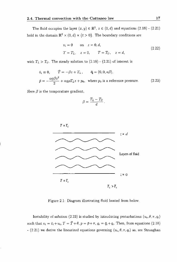
2.4. T h e r m a l convection wi th the Cat taneo law 17
The fluid occupies the layer {x,y) e R ^ , 2 G {0,d) and equations (2.18) - (2.21)
hold in the domain x ( 0 , r f ) x {t > 0 } . The boundary conditions are
Vi = 0 on z — 0,d,
T = T L , 2 = 0, T = Tu, z = d,
wi th TL > Ty. The steady solution to (2.18) - (2.21) of interest is
v, = 0, f=-pz + n, q = ( 0 , 0 , K / 3 ) ,
agPz' 2
+ agpTiZ + pq, where po is a reference pressure.
Here P is the temperature gradient,
TL-TU
(2.22)
(2.23)
T=T..
T = T,,
= d
Lavers of fluid
;= 0
Figure 2.1: Diagram il lustrating fluid heated f rom below.
Instabili ty of solution (2.23) is studied by introducing perturbations (u j , 6', T T , ^ j )
such that Vi = Vi + Ui, T = f + 9, p = p + n, Qi = Qi + Qi- Then, f rom equations (2.18)
- (2.21) we derive the hnearized equations governing (wj, ^, T T , q-j) as, see Straughan

2.4. T h e r m a l convection w i t h the Cat taneo law 18
& Pranchi [173],
Uit = — 7 r , j + agki9 + vAui, P
= °' (2.24)
r(9i ,t - ^Ui^zK'P + ^«/?^«,z) = -Qi - >
where it; = U3. Equations (2.24) are non-dimensionalized as in Straughan & Pranchi
173]. We need the Prandt l number, P r , Cattaneo number, C, and Rayleigh number,
Ra = R^, which are
(2.25)
The non-dimensional linearized equations (2.24) are
•Uj,t = —TT j - I - Rki9 + A i i j ,
Ui,i = 0,
Pr9t = Rw-
2CPrqi^t = -Qi + CR{ui^, - ^^;,^) - 9,i.
To study instabili ty we seek an exponential t ime dependence like
zxi(x, t) = e'^'uiix), 9ix, t) = e'^*^(x), gi(x, t) = e^'gi(x), 7r(x, t) = e '^V(x),
Equations (2.25) yield
aUi = —7r_j + RkiO + A u j ,
= 0, (2.26)
oPr9 = —
2aCPrqi = - g , + Ci?(wi,^ - t/;,i) - .
Ehminate T T f rom (2.26)i and put Q = Qi^t, where " _ i " means derivative wi th
respect to a;,. Thus we solve the equations
a Aw = RA*9 + A^w
aPr9 = Rw-Q (2.27)
2aCPrQ =-Q - A9 - CRAw ,

2.4. T h e r m a l convection wi th the Cat taneo \aw 19
where A* = d'^/dx'^ + d'^/dy'^ is the horizontal Laplacian.
We now use the D'^ Chebyshev tau numerical method to solve equations (2.27).
The fixed surface boundary conditions are
w = w, = 9 = 0, z = 0,l. (2.28)
Equation (2.27)i is four th order and hence we introduce the variable x by X =
We let / be a plane t i l ing periodic function so that f^x + fyy = - a ^ / where a is a
wavenumber. Next wri te it;, x, 9 and Q in the form
w^W{z)f{x,y), x = x{z)f{x,y), 9 = e { z ) f { x , y ) , Q = Q{z)f{x,y).
We now solve (2.27) as
{D^ - a^)W - X = 0,
{D' - a')x - Ra'e = ax, (2.29)
(D^ - a^)Q + Q + CRx = -2aCPrQ,
Q-RW = -aPrO.
The functions W, x, © and Q are expanded in terms of Chebyshev polynomials, for
yv odd, N N
W{Z) = ^WnTniz), X{Z) = ^XnTn{z), n=0 n=0 N N
Q{Z) = J2QnTn{z), Q{Z) ^^QnTniz). n=0 n=0
To use the boundary conditions (2.28) we note that
7 ; ( ± 1 ) = ( ± 1 ) " , T ^ ( ± l ) = {±ir-'n\
Then the boundary conditions (2.28) become, i=N-l i=N
^ Wi = 0, ^Wi = 0, (2.30) i=0 i = l
i even i odd
i=N-l i=N
i^Wi = 0, ^^^i = 0' (2.31) 1=2 i = l even i odd
=N-l i=N
5 0 , - 0 , ^ e , = 0. (2.32) i=0 1=1
i even i odd

2.4. T h e r m a l convection w i t h the Cat taneo law 20
The Chebyshev tau method now reduces to solving the matr ix system A x = aBx.
Here the (A^ + 1) x (A^ + 1) matrices A and B are given by
A =
BCl
BC2
0
BC3
BC\
0
0 . . . 0
0 . . . 0
y -RI
( 0
0 . . . 0
0 . . . 0
0
0 . . . 0
0 . . . 0 B =
0
0 . . . 0
0 . . . 0
0
- /
0 . . . 0
0 . . . 0
4D^ - o?I
0 . . . 0
0 . . . 0
CRI
0 . . . 0
0 . . . 0
0
0
0 . . . 0
0 . . . 0
/
0 . . . 0
0 . . . 0
0
0 . . . 0
0 . . . 0
0
0
0 . . . 0
0 . . . 0
-Ra?I
0 . . . 0
0 . . . 0
4L>2 _
BC5
BC6
0 \
0 . . . 0
0 . . . 0
0
0 . . . 0
0 . . . 0
/
0 . . . 0
0 . . . 0
0
0
0 . . . 0
0 . . . 0
0
0 . . . 0
0 . . . 0
0
0 . . . 0
0 . . . 0
-PrI
0 \
0 . . . 0
0 . . . 0
0
0 . . . 0
0 . . . 0
-2CPrl
0 . . . 0
0 . . . 0
0
where x = [WQ, . . . , IVAT, XO, • • •, X N , ©O, • • •, © N , <3O, • • •, QN)- The boundary condi
tions BCl,BC2, BC3,BCA, BC5,BC6 refer respectively to (2.30), (2.31), (2.32).
The matr ix system is solved by the QZ algorithm used as given in the N A G library,

2.5. N u m e r i c a l results 21
cf. Dongarra et al. [41]. Note that in the last block row of A and B there are no boundary conditions. This is due to the fact that (2.29)^ is an identity and not a differential equation.
2.5 Numerical results
Straughan and FYanchi [173] found that for two free surfaces, the following asymp
totic formula,
R a = ^ ( l + ^C7r' + 0{C') 4 V 2
We present numerical results for two fixed surfaces below. Again, we f ind Ra to be
increasing in C.
Table 2.1: Cri t ical Rayleigh numbers
c i?a a
0 1707.765 3.12
10-^ 1711.180 3.12
2 X 10" -4 1714.596 3.11
4 X 10" -4 1721.475 3.11
6 X 10" -4 1728.402 3.10
8 X 10" -4 1735.369 3.10
10-2 1742.393 3.09
2 X 10" -3 1778.194 3.07
4 X 10" -3 1853.544 3.03
6 X 10" -3 1934.276 2.98
8 X 10" -3 2020.868 2.94
10-2 2113.893 2.89

2.5. N u m e r i c a l results 22
The results in this table we found by fixing and solving for a. The numerical routine seeks that value of Ra for which Rea = 0. Then we find
min Ra{a^). a?
I t was found that a £ M throughout the table. Prom the table we see that Ra
satisfies an approximately linear relationship in C. For small C values we have
Ra ~ 1707.765 - I - 34150C (2.33)
so the slope is approximately 3.5 bigger than that in the free surface case.

Chapter 3
Green and Laws model
3.1 Derivation of the model
I n this section we wi l l summarize the derivation of the model which appeared in
Green and Laws [58 .
In the article of Green & Laws [58], they proposed the entropy production in
equality for the whole body b and for the material volumes p, by employing the
specific Helmholtz free energy and energy equation together w i t h other standard
balance equations. Moreover, they make the constitutive assumptions that •0,77, (j), Qi
are functions of 9,6,9^i. Furthermore, they treat both the external volume and sur
face supplies of entropy on an equal footing and retain a non-zero r . The balance
laws for a single phase continuum that are used in Green &: Laws [58] are
p + pvi^i = 0 (3.1)
tki,k + pFi = pVi, (3.2)
pr - Qi^i + tikdik - pi = 0, (3.3)
where p,Vi,tki,Fi,r,qi and £, are, respectively the mass density, the velocity, the
Cauchy stress tensor, the specific body force, the specific heat supply, the heat flux
and the specific internal energy. The stress tensor Uk is symmetric, so tik — t^i,
and dik is the symmetric part of the velocity gradient, dik = |(vi,fc + Vk^i). Also a
superposed dot denotes material t ime differentiation.
23

3.1. Der ivat ion of the model 24
In 1967, MuUer [121] proposed an entropy production inequality of the fo rm
4- I PVdv - / ^dv + [ kiUida > 0 (3.4)
for every material volume p, T] is the specific entropy, 9 is the absolute temperature
{9 > 0), ki is an entropy flux vector, and n j is the outward unit normal to the
boundary surface, dp, of p.
The equation of motion (3.2) and the energy equation (3.3) are balanced by suitable
choices of body forces Fj and heat supply r.
Green & Laws [59] suggest that since (3.4) holds for every material volume p, i t also
holds for the whole body b, therefore they assume that the only external volume
supply of entropy is defined in a particular way in terms of externally supplied rate
of production of heat r , namely r/9. Similarly the only external supply of entropy
over the boundary db of the continuum is that defined in the same way in terms of
the rate of supply of heat. Then they suggest that the entropy flux vector in (3.4)
be restricted by the condition
kiUi = on db. (3.5) u
Otherwise the external supply of entropy over db is of different character f rom the
external volume supply of entropy.
In 1971, Muller [123], [122] considered solutions of (3.1) to (3.3) when Fj = 0, r = 0.
Green & Laws [58] assume that associated w i t h the heat supply r there is an entropy
supply r / 0 where cj) > 0 and 0 = ^ in equihbrium. The function (p = 4>[9,9) is a
generalised temperature.
For the whole body 6, the entropy production inequality is
f PVdv - f ^ d v + [ ^ d x > 0, (3.6) dt Jb Jb 4> Jdb <P
and for all material volumes p, the entropy production inequality is
^ Iprjdv - [^dv+ [ ^ d x > 0. (3.7) dt Jp Jp 4> J dp 0
Green & Laws [58] deflne the Helmholtz free energy ip = e — 770, and consider a
stationary rigid heat conductor. Moreover, they use the constitutive assumptions

3.1. Der ivat ion of the model 25
that ijj,r],(t),qi are functions of 9,6,0^i, and exploit the Helmholtz free energy -tp
together w i t h the constitutive assumptions into (3.7) to obtain
= 0 (which yields (j) = (p{e, 6)),
For a rigid sohd which conducts heat according to a Fourier law
Qi = -iiij{9,9)9j,
(3.8)
(3.9)
leads to Kij is symmetric.
Define equilibrium to be when ^ = 0, 9^i = 0, and let (pls = 9, hence {0(p/09) \ =
1. Then Green & Laws [58] show
V\E =
and -
09
dqi
d9,j
n = 0,
is a positive semi-definite tensor. (3.10)
By employing (3.7) and the Helmholtz free energy: = e - rjcp, then the equation
(3.3) becomes
pr - Qi,, - p{tP + + (f>rj) = 0, (3.11)
and the linearized version of (3.11) is
pr Oqi
09
09
Oqj 09,
9
E \ C't'.i 9i = 0. (3.12)
Thus, (3.12) is capable of predicting a finite speed of heat propagation. We now
study the properties of a solution to equation (3.12) in some detail.
Throughout the remainder of the thesis Q w i l l denote a domain in M''. I f has
a boundary this wi l l be denoted by P.

3.2. Uniqueness for the G r e e n and L a w s model w i th kj constant 26
3.2 Uniqueness for the Green and Laws model with ki constant
In this section C M" is a bounded domain w i t h boundary F. Now, discuss equation
(3.12) and take the specific heat supply r = 0 then this equation becomes,
where the coefficients are
(3.13)
a = p\4>
dqi
dqi.
89
drj
In this section a,/?,.^ifc and h are constants, we assume ifc to be symmetric, and
equation (3.13) holds on the domain f2, t > 0.
The boundary and ini t ia l conditions are
Boundary Condition
In i t ia l Conditions
e = f[x,t)onT, (3.14)
e{x, 0) = g{x), 9t{x, 0) = h{x), x e n. (3.15)
Let P denote the boundary-init ial value problem given by (3.13)-(3.15).
To prove that the solution is unique, assume that there are 2 solutions 9^ and ^2
which satisfy the equation (3.13) and the boundary-init ial conditions (3.14) and
(3.15). Then let w ^ 9i - 9^. Prom (3.13) we find w satisfies
ail) -\- (3w -\- ^ikW^ki + hy^^i ~ 0, where x eVl, t > 0,
wi th the boundary condition
and the in i t ia l conditions
w = 0 on r ,
(3.16)
(3.17)
w{x,0) = 0, xeQ, (3.18)

3.2. Uniqueness for the G r e e n and L a w s model w i th kt constant 27
wt{x,0) = 0, xen. (3.19) To demonstrate uniqueness we mult iply (3.16) by lii and integrate over Q, to obtain
a / wwdx + P w^dx + I ^ikW^ikwdx + / kiWiwdx = 0, (3.20) Jn Jn Jn ' Jn '
or equivalently in the form,
a{w, w) + p{w, w) + i^ikw^ki, w) + {kiW^i, w) = 0, (3.21)
where (•, •) denotes the inner product on L'^{Q). Note that
a(w,iu) = a [ wwdx = ^ [ •^(w)^dx = ^-^Ww (3.22) JQ ^ Jn dt 2 at
The second term of (3.21) is
P{w, w) = P I w^dx = P\\wf, (3.23) Jn
and for the ki term we have
{kiW^i,w) = / kiW^iwdx Jn
= I h-Jn <
d'^w 9w ^ ' dxidt dt
2
= L2d^\-m) '''^"S the chain rule
1 / 5 r f d w Y ] , . ^ . ^ 2 J dx' \dt J ^^^^^ ^ constant vector
= 2 y '^ihi-Q^f'ds.hy using the divergence theorem
= 0. (3.24)
For the term,
(^ikW,ki,U!) = / ^ikW^kiWdx Jn
= / ^ikw[^w^i)dx Jn oxk
= Uk^ikWtW^ids - J ^ikW^iW^kidx,

3.2. Uniqueness for the G r e e n and L a w s model w i th ki constant 28
where we have integrated by parts and used the divergence theorem. The first term is zero since u' = 0 on F, so that
{^ik'w,ki,w) = - / ^ikW^iW^ktdx, Jo.
= - ~ y iikW,iW^kdx. (3.25)
Employing (3.22) to (3.25) in (3.21), equation (3.21) becomes
a d 2dr " - J j , k W , w , k d x = 0, (3.26)
or a d 2Jt
f v?dx + P f w^dx - ~ [ iikW^iW^kdx = 0. (3.27)
Integrate equation (3.26) f rom 0 to t,
~ [ (aw'^-^^kWiWk^dx + P [ [w^dx = 0. (3.28) ^ i n \ / Jo Jn
We now require a > 0, /? > 0, ^ik to be a negative semi-definite tensor, i.e.
^tkUk < 0, that is
^i^k < 0, v^, . C ,fe E
Then f rom equation (3.28) we obtain
0 < - / aw - ^ikW^.w^k ]dx<Q, In
and so
0 <a w^dx - / S,ikW iW kdx < 0. Jn Jn
Since a w'^dx > 0 and — ^ikW^iW^kdx > 0, then
0<a I w^dx < 0. (3.29) Jn
Therefore
/ w^dx = 0, (3.30) i n
so ti; = 0, this leads to = 0, hence 9i = 92 which yields uniqueness.

3.3. Uniqueness for G r e e n and L a w s model wi th ki = ki{x) 29
3.3 Uniqueness for Green and Laws model with
Now we use equation (3.13) but allow fcj to depend on the spatial variable, i.e.
ki = ki{x). Let 9i and ^2 be solutions to the boundary-init ial value problem defined
by equations (3.13),(3.14) and (3.15), where 9i and 62 each satisfy (3.14) and (3.15)
for the same data functions / , g and h.
Let w = 9i — 92- Then from equations (3.13),(3.14) and (3.15) we find w sat
isfies the boundary-init ial value problem (3.16), (3.17) and (3.18). We now, prove
uniqueness when A;, = ki{x).
M u l t i p l y (3.16) by w and integrate over the domain Q. Thus
a / wwdx + P / {'w)'^dx + / S,ik'w,kiwdx + I kiiii^iwdx = 0. (3.31) Jn Jn ' Jn '
As in section (2.2) we find
a f wwdx = ^ - ^ I k l P , (3.32) Jn 2 dt
and
J iikWMUJdx = J E^ikW^iW^kdx (3.33)
For the te rm in ki we note
/ kiWiwdx= ! ^4-{^?dx (3.34) Jn ' Jn ^ Oxi
and upon integration by parts
f kiWiwdx=- f -^(kiW^)dx ~ [ ^w^dx JQ ' 2Jn0xi^ Ja 2
= ^ / n^kiw'^ds-]- I kiiw'^dx 2 Jv 2 '
= - \ ! ki^iw'dx, (3.35) ^ Jn
because ti; = 0 on F.
Then, employing equation (3.32)-(3.35) in equation (3.31) we obtain
1 d J ^ikW,iW,kdx^ ^ i i (' ~ ^ ) ' '' ' " °' ^ ' ^

3.4. Cont inuous dependence of the thermal energy 30
We now require that
/ 3 - ^ f c i , i ( x ) > 0, V X G Q . (3.37)
Then we discard the /? - A:i,i/2 term in (3.36) to find
| < 0 . (3.38)
Integrate this f rom 0 to i to find
^ l l ^ ^ f / iikw^^^kdx<^, (3.39) ^ ^ Jo.
since ii;(a;,0) = 0 and w{x, 0) = 0. Since iikii^k < 0 inequality (3.39) leads to
0 < | | w ( i ) | | 2 < 0 (3.40)
Therefore
| | i i ; ( i ) | | = 0. (3.41)
Thus
10 = 0 i n Q , V t (3.42)
and so
w{x,t) = ^. (3.43)
Hence the solution 9 to the boundary-initial value problem (3.13),(3.14) and (3.15)
is unique.
3.4 Continuous dependence of the thermal energy
I n this section we suppose ki = ki{x).
We now suppose 9 satisfies the boundary and ini t ia l conditions
^ = 0 on r, ^ ( x , 0 ) = 9o{x),xe Q,
9{x,0) = 'po{x),x e Q.
Then mul t ip ly equation (3.13) by 9 and integrate over Q, we obtain,
a{9, B) + (5{9,9) + ( ^ - ^ . ^ i , 9) + {h{x)9^u 9) = 0. (3.44)

3.4. Cont inuous dependence of the thermal energy 31
We note,
{^rk9,ik.9) = I U&,ik9dx Jn
= (3.45)
as in Section (3.3) we find
{h{x)9,J) = -\j^kJ^dx. (3.46)
Employing (3.45) and (3.46) into (3.44), we obtain
^ ± f e^dx + (5 [ 9 ' d x - ~ [ ^ik9Akdx-l [ k j ' d x . (3.47) 2 dt Jn JQ dtz Jn 2. Jn
Rearranging equation (3.47), we obtain
Suppose now
/? - ^ > /3o > 0. (3.49)
Then f rom equation (3.48) we have
It In " \^^>^^^^^'>) " " + ^° X ~ ° ' ^^'^^^
Integrate f rom 0 to i over f i , we obtain / ^0'dx-\ ! ^ik9Akdx + Po f [ 9'dxdT)
Jn Jn Jo Jn < ^ j j l d x - \ j j i k 9 ' , 9 % d x . (3.51)
Suppose
^ikriiTlk < 0, (3.52)
then
- / ^ik9,r9,kdx > 0. (3.53) Jn
Therefore, f rom equality (3.51) we have
^ / 9^dx + (3o f [ 9^dxdri < Do, (3.54) 2 Jn Jo Jn

3.5. Uniqueness and continuous dependence for a related model 32
where DQ is the data term,
Do = ^ [ ^Idx - \ I E,^k9''i9\dx + Po f ! ^o'dxdrj. (3.55) ^ Jn Jn Jo Jn
Define now
F{t) = f f 9^dxdr], thus F'{t) = [ 9^dx. (3.56) Jo Jn Jn
Then the equahty (3.54) may be rearranged as
2
or
^F'it)+0oF{t)<Do, (3.57)
F'{t) + ^ F ( 0 < -Do. (3.58) a a
M u l t i p l y (3.58) by e x p ( ^ ) , then we have
d Mm ^\ ^ 2 20ai e . F <-e.'D„.
Then integrating
^'F{t) - F (0) < / -Doe'^^ds Jo »
rearranging to obtain.
a J \2jJo
e - ^ ' F ( i ) < F(0) + -r^ e ^ ' - \ Po
So
F ( t ) < | ( l - e - ^ ) (3.59)
Inequality (3.59) shows continous dependence of 9 on the in i t ia l data in the F{t)
measure.
3.5 Uniqueness and continuous dependence for a
related model
A n equation very similar to (3.13) may be taken f rom the work of Payne & Song
134]. These authors study a model for thermoelasticity which stems f rom the ther
modynamic treatment of Green &; Laws [58]. By fixing the displacement, Uj, in

3.5. Uniqueness and continuous dependence for a related model 33
equation (1.11) of Payne & Song [134] so that i t j j = 0, one arrives at the equation for the temperature field 9 of form
h9 + de- biO^i - {bi9)^, = ikik9,k)4- (3-60)
Clearly equation (3.60) is very like our equation (3.13) but has the extra term
In this section we establish uniqueness and continuous dependence on the in i t ia l
data for a solution to (3.60). Hence, let Q C M"* be a bounded domain wi th boundary
r and suppose (3.60) is defined on the space-time domain x (0, T) for some T > 0.
The boundary conditions are
9{x,t) = f { x , t ) , x e r , (3.61)
and the in i t ia l conditions are '
9{x,0) = g{x), 9t{x,0) = h{x), (3.62)
where a; e
The functions h,d may depend on x but h > 0,d > 0,bi = bi{x) and kij = kij{x),
but kij^i^j > 0, V^.
To estabhsh uniqueness and continuous dependence we let 9i and ^2 be solutions
to (3.60) and (3.61) for the same data function / . Let 9i satisfy (3.62) for g =
gi,h = hi and let ^2 satisfy (3.62) for g = g2,h = /i2- Define w = 9i - 92,G =
Qi — g2, H = hi — h2, then f rom (3.60)-(3.62) we find w satisfies the boundary-initial
value problem
hw + dw - biW^i - {biib)^i = {kijWj)^i, in fl x (0, T ) , (3.63)
w{x,t) = 0, x e r , (3.64)
w{x, 0) = G{x), wt{x, 0) = H{x), x e n . (3.65)
M u l t i p l y equation (3.63) by w and integrate over to find
/ hw'^dx+ [ dw'^dx+^]- f kijW jdx dt 2 JQ JQ dt2
= / biWWidx^- I {biw)iwdx, (3.66) Jn ' . Jn

3.5. Uniqueness and continuous dependence for a related model 34
where we have integrated by parts on the kij term and used the boundary condition. To handle the right hand side we use the chain rule and integrate by parts to see that
/ biww^idx + / {hiw)^iwdx Jn ' Jn '
= - bi{w'^)^idx+ / biW^iwdx + / bi^iw'^dx 2 Jn ' Jn ' Jn '
= [ bi{w'^) idx + I- I bi{w^)^idx+ [ bi^iW^dx 2 Jn ' 2 i n ' JQ
= / bi{'uP')^idx + I bi^iW^dx Jn ' Jn '
= J biUiW^dS = 0, (3.67)
since l i ; = 0 on F. Thus, equation (3.66) becomes
[ hw^dx + l f kijWiWjdx]+ [ dw^dx = 0. (3.68) dt\2 JQ 2 JQ ' ' / Jn
Since rf > 0 we drop the last term to obtain
^( [ hw^dx+ I kijWiWjdx] < 0. (3.69) dt\Jn Jn ' ' /
This equation is integrated f rom 0 to i and we find
! h[w{x,t)fdx+ I kijW^i{x,t)wj{x,t)dx < / hH^dx+ / kijG^iGjdx. (3.70) Jn Jn ' ' Jn Jn
Inequality (3.70) yields continuous dependence on the in i t ia l data g and h in the
measure
E{t) = / h[w{x,t)]'^dx + / ki. jW^i{x,t)wj{x,t)dx. (3.71) Jn Jn ' '
I f we additionally know kij is positive-definite, i.e.
hjUj > ^ o l ^ l ' , ko > 0, (3.72)
then since h > 0 we may deduce f rom (3.70) w i th the aid of Poincare's inequality
that
koXi I [w{x,t)fdx< I hH^dx+ f kijG^iGjdx, (3.73) Jn Jn Jn '

3.6. A n instabi l i ty result for a solution to (3.13) 35
where Aj > 0 is the constant in Poincare's inequality.
Inequality (3.73) demonstrates continuous dependence on the in i t ia l data g and
h, in the L ^ ( f i ) measure of w, and hence 9.
Uniqueness follows immediately f rom (3.73) when (3.72) holds, for in that case
G = 0, / / = 0 and so f rom (3.73)
0 < / w'^dx < 0 < / w^dx < 0 (3.74) Jn
which shows to = 0 V ( x , t ) ' e 0. x (0, T ) . Thus 9i = ^2 and hence uniqueness.
When kij is simply positive, i.e. fcjj^iCj > 0, then uniqueness follows f r o m (3.70). In
that case we see
0 < / hw^dx < 0 (3.75) Jn
and since h > 0 we must have u; = 0 in Q x ( 0 , T ) . I t then follows w = 0 and so
9i = 92 in Q X ( 0 , T ) , hence uniqueness.
3.6 A n instability result for a solution to (3.13)
We return now to equation (3.13) which we recollect together w i th the boundary
and in i t ia l data as
a9 + p9 + UO,ik + ki9,i = 0, in n X (0, oo), (3.76)
9{x,t) = 0, x e r , (3.77)
9{x, 0) = g{x), 9t{x, 0) = h{x), x e n. (3.78)
In this case we assume o;, (3 are constants but allow fcj to depend on x.
Our aim is to see whether the continuous dependence (stability) result of Section
3.4 may be negated if ki is sufficiently large and ^ij is not negative. Thus, mult iply
(3.76) by 9 and integrate over Q.. Af ter calculations like those of Section 3.4 we may
show that
si L'''' -IM-')^ 5 /„
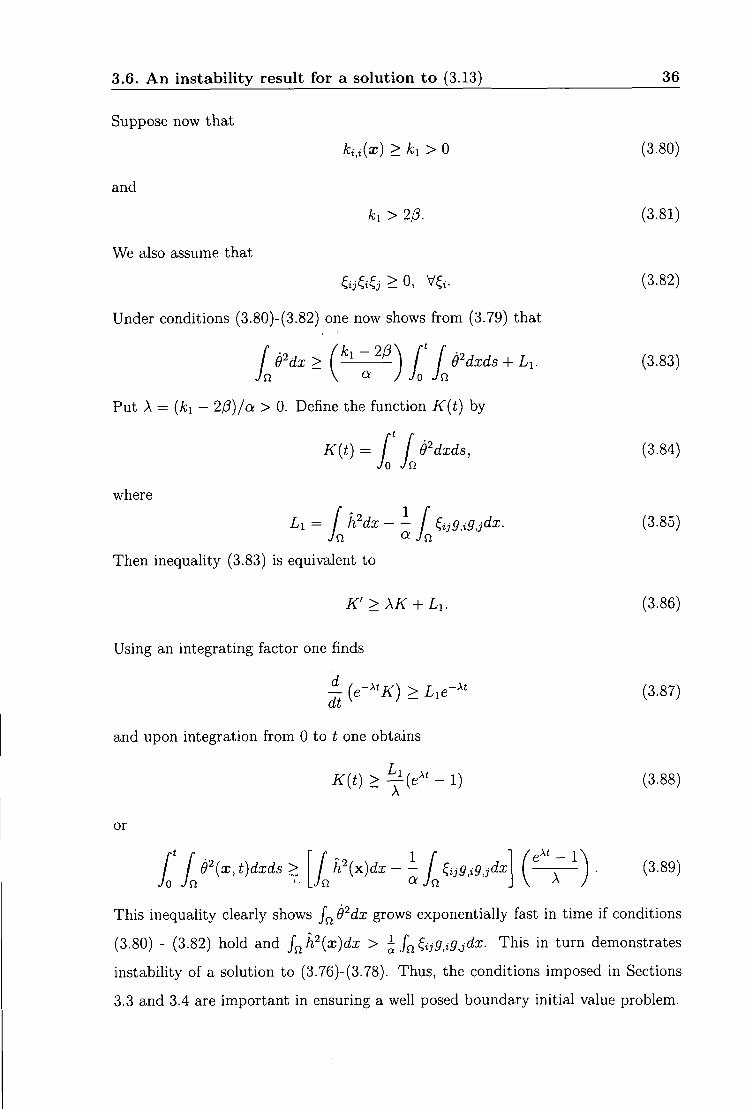
3.6. A n instabil i ty result for a solution to (3.13) 36
Suppose now that
and
We also assume that
k^,^{x) >ki>0 (3.80)
ki > 2p. (3.81)
Under conditions (3.80)-(3.82) one now shows f rom (3.79) that I
J eHx > £ J O'dxds + L i . (3.83)
Put A = (fci - 2P)/a > 0. Define the function K{t) by
K{t) = f [ 9^dxds, (3.84) Jo Jn
where
Li= f h^dx I ^ijg^iQjdx. (3.85) Jn <^ Jn
Then inequality (3.83) is equivalent to
K'>XK + Li. (3.86)
Using an integrating factor one finds
I {e-''K) > L,e-'' (3.87)
and upon integration f rom 0 to ^ one obtains
K{t)>^[e^' - \ ) (3.88)
or
j ' ^ j 9^{x,t)dxds> I h\x)dx-^ J ^ijg^iQjdx • (3-89)
This inequality clearly shows 9'^dx grows exponentially fast in time if conditions
(3.80) - (3.82) hold and J^ h?{x)dx > ^ j Q ^ i j g , i g , j d x . This in tu rn demonstrates
instabili ty of a solution to (3.76)-(3.78). Thus, the conditions imposed in Sections
3.3 and 3.4 are important in ensuring a well posed boundary ini t ia l value problem.
3.7. Uniqueness on an unbounded spat ia l domain 37
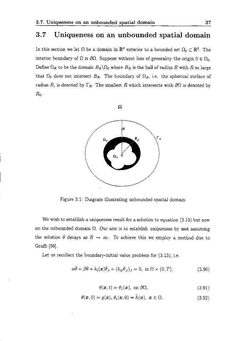
3.7 Uniqueness on an unbounded spatial domain
In this section we let be a domain in exterior to a bounded set J o C R^. The
interior boundary of f ] is Suppose wi thout loss of generality the origin 0 e QQ-
Define Q/j to be the domain BRXCIQ where Bn is the ball of radius R w i t h R so large
that CIQ does not intersect BR. The boundary of 0,^, i.e. the spherical surface of
radius R, is denoted by Ff l . The smallest R which intersects w i th dQ is denoted by
Ro.
Figure 3.1: Diagram il lustrating unbounded spatial domain
We wish to estabhsh a uniqueness result for a solution to equation (3.13) but now
on the unbounded domain Q. Our aim is to establish uniqueness by not assuming
the solution 9 decays as —> oo. To achieve this we employ a method due to
GraflS [56 .
Let us recollect the boundary-initial value problem for (3.13), i.e.
a9 + P9 + ki{x)9,i + {kij9,j),i = 0, in Q x (0, T), (3.90)
9{x,t) = 9i{x)\ on dn,
9{x,0) = g{x),9t{x,0) = hix), x e Q.
(3.91)
(3.92)

3.7. Uniqueness on an unbounded spatial domain 38
To establish uniqueness via the Graff i method we assume 9i and ^2 are solutions
to (3.90)-(3.92) for the same data functions 9i,g and h. Let w = 9i - 6*2. Then w
satisfies the boundary-init ial value problem,
aw + Pw + ki{x)w,i + {kijWj),i = 0, x e te{0,T), (3.93)
w{x,t) = 0, X e on, (3.94)
w{x, 0) = 0, wtix, 0) = 0, x e n . (3.95)
Mul t ip ly equation (3.93) by w and integrate over for R fixed. We find
[ i ^w^ — iW j ] dx + f kijW iWUjdS dt JnR\2 2 ' ' J
+ / pw-dx+ f '^iw^),idx = 0, (3.96) Jnn Jnn 2
where we have integrated by parts on the % term. For the last term
/ '^{w'),dx^ [ ^ w ' d S - [ ^w'dx. (3.97) JnR 2 J^^ z Jn^ z
Combining (3.97) w i t h (3.96) we see that
= - / (kijnjWWi+ " ^ w A dS. (3.98)
Integrate equation (3.98) twice over the t ime region (0, T ) ,
/ [ (—w'^ - l - k i j W iW j \ dxdrj + [ [ f (P - w'^dxdp,dr] Jo Jna\2 2 ' ' J Jo Jo JnnK 2 J
= - f I I (kijrijWWi + ^w^^dSdij^dr]. (3.99) Jo Jo JFRK ' 2 /
We now require
/ 3 - ^ . > 0 . (3.100)
Then the term P — ^ may be dropped, hence we obtain
Jo Jnn\2 2 J m ( kn- \
kijnjww,i + -^w^ dSdiidr]. (3.101) H V 2 J
3.7. Uniqueness on an unbounded spatial domain 39
We now suppose kij is a bounded, negative-definite tensor, so that
-kijUj > ao\^\\ ao > 0. (3.102)
By employing (3.102) in (3.101), we then obtain
J J (^^'^^ + ^oiow^iW^^ dxdr]
~~Io lo I (^^^^^'^^'^ + " ^ ^ ^ ) (3.103)
Suppose \kij\ < K, \ki\ < ki, fci > 0, then we obtain
^ / / ctow^iw^^^ dxdr)
We then use the arithmetic-geometric mean inequality on the right to see that
^ lo I ( ^ ocQW^iW^i^ dxdr]
or,
\ i I f ^ ^ ^ + oiQW^iW^^ dxdr} 2 Jo JUR ^2 /
< [ [ I ( ^ H ^ + l ^ ) < i 5 d ^ d , ^ (3.106)
Hence, we obtain
i f I {aw^ + aow,w,)dxdr, < i ^ ± A E T / {\w\'+ \Vwf) dSd^. 2 Jo JQR 2 Jo Jvn
(3.107)
Let ai = min{Q;,Q!o}, then
^ r f {w' + \^w\') dxdrj 2 Jo JQR
- \ f f i^'^^ + ao\Vw\^) dxdr] 2 Jo JUR n {\wf + \Vw\^) dSdr],
- R
^ {K + ky)T

3.7. Uniqueness on an unbounded spatial domain 40
or
a, / / {w^ + \Vw\^)dxdri<{K + k,)T [ f {\wf + \Vwf) dSdv- (3.108) Jo JUR JO JTR
Define now
F{R)= ! I [w'' + \Vw\^)dxdr}, (3.109) Jo JQR
and put A = ai/{K + k-i)T. FYom inequality (3.108) one shows
A F < ^ . (3.U0)
Thus,
^ [ F e x p ( - A / ? ) ] > 0 .
Integrate this from 0 < i?o to /? to find
F{R) > F(i?o) exp[A(i? - RQ)]. (3.111)
Suppose now that our class of solutions is such that
\w\, \Vw\ < e^'^ for some ^ > 0. (3.112)
Then, since F{RQ) = FQ is a constant (3.111) shows that
Foexp[A(/i: - i?o)] < F{R) < Ae^^'^, (3.113)
some A> 0. If we pick T small enough then (3.113) yields a contradiction, i.e. for
A > 2 ^ ,
or ai
2aK + hy Thus, w = 0 onfl X (0, T) and uniqueness follows.
However the bound (3.112) is independent of T and so we may repeat this argu
ment on (T, 2T), and so on to establish uniqueness on (0, T) .
N.B. The original Graffi method, see Graffi [56], was developed for the Navier-
Stokes equations and for the equations of compressible flow. The extension of the
Graffi method to hyperbolic equations of linear elasticity was due to Straughan [167 .
3.8. A non-standard problem for equation (3.13) 41
3.8 A non-standard problem for equation (3.13)
Payne & Schaefer [127] began a study into non-standard problems for a class of
partial differential equations. They argued that rather than prescribe initial condi
tions on the function, d, say, one prescribes a combination of the solution at i = 0
and at f = r , for some time T > 0. Such a class of problem may be employed to
obtain bounds for the solution when the problem is improperly posed. The class of
non-standard problems studied by Payne k. Schaefer [127] has proved to be a very
frui t fu l area of research as may be witnessed by the extensions of Ames & Payne [3],
Payne et al. [128,129], Ames et al. [4,5], and Quintanilla & Straughan [153,154 .
To state the class of non-standard problem we are interested in, suppose in (3.13)
we change a to m, /? to d, ^tj to -ctij and for m,d> 0 but constant we have
me + de + ki{x)9,i - {ocijej)^i = o. (3.114)
Equation (3.114) holds in h x (0, T) where Q e is bounded. On the boundary
of Q, r , we have
e{x,t) = 0, x e r . (3.115)
For constants a, /3, the "initial" conditions are replaced by
a9{x,O) + 0{x,T)=g,
p9t{x,0)-\-9t{x,T) = h, xen. (3.116)
Our goal is to establish that a solution to (3.114)-(3.116) depends continuously
in an appropriate manner on the data functions g and h. To achieve this we begin
with a general estimate which follows by multiplying (3.114) by 9 and integrating
over Q. After integration by parts and use of the boundary condition (3.115) we
may arrive at
r / ( d - ^ ) 9 ' d x d r j + l f a,,9,{t)9,{t)dx 2 Jo Jn\ 2 y 2
= y l l ^ ( 0 ) | | ' + ^ a . , ^ , ( 0 ) ^ , ( 0 ) d x , (3.117)
where here and throughout this section we have suppressed the dependence on x in
9.

3.8. A non-standard problem for equation (3.13) 42
Observe that (3.117) does not by itself yield a continuous dependence estimate for 9{t) since the right hand side consists of unknown functions ^(0), V^(0). We do not know 6{x,0),0{x,0) we only know the data functions g{x) and h{x).
We suppose throughout this section that
d - ^ > 0 \fxeQ.
\al\P\ > 1.
We firstly consider the case |Q;|, \P\ > 1. Thus, we evaluate (3.117) for t = T and
drop the second term on the left of (3.117). This yields
m | | ^ ( T ) f + / a,je,,{T)e,{T)dx Jn
<m| |^(0) | |2+ f aij9j{0)eii0)dx. (3.118)
Now, use equation (3.116) in the left hand side of (3.118) to find
m{h - Pd{0), h - pe{0)) + f aij[gj - aej{0)][g,i - a0,^iO)]dx Jn
<m\\e{0)f+ [ aij9j{0)ei{0)dx, (3.119) JQ
where (.,.) denotes the inner product on L^(Q).
Note now that
{h - petiO), h - P9t{0)) = \\hf + P'\mo)f - 2/3(/i, ^,(0))
> \\hr+p'\mQ)f - ^\mo)r - ewh^, (3.120)
for e > 0, where we have used the arithmetic-geometric mean inequality. For £i > 0
we similarly establish
JQ
= f cyijgjg,idx + I aij9ji0)9,i{0)dx - 2a I aijg^,9j{0)dx, Jn Jn Jn
> [ (x,jg^igjdx + a' [ ai,-^,,(0)^,,(0)rfx Jn Jn
- — I a , ,0i(O)0, ,(O)dx-£i [ aijg,ig,jdx. (3.121) ^1 Jn Jn

3.8. A non-standard problem for equation (3.13) 43
Combining (3.120) and (3.121) in (3.119) we thus obtain
m/?2 (l - -] 11 4(0)11" + a ^ ( l - - ] [ ai^ei{0)9 jiO)dx \ \ £\J Ja
+ m ( l - £)||/i||^ + (1 - £i) / Ciijg,ig,jdx Jn
< m | | ^ t ( 0 ) | p + / aij9,i{0)9,j{0)dx. (3.122) Jn
Since |/3| > 1, |Q;| > 1 we choose
e = -z—- > 1 and £i = — - > 1.
These choices in (3.122) yield the inequality
m ( ^ ^ ) ll^t(0)|| ' + ( ^ ^ ) J ^ c . ^ A ^ m M d x
^ ^ ll^ll + / (3-123)
Put ^ = min{|a | , and then from (3.123) we may obtain
m| |^t(0) |P+ [ aij^,i(0)^,^(0)dx Jn
<h\\h\\^ + k2 I cxijg,ig,jdx, (3.124) Jn
where
^ . = ™ ( ^ ) ( ^ ) > o . * ^ = ( ^ ^ ) i ^ ; > o . Finally, employ the bound (3.124) in (3.117) to find
< V I I ^ I I ' + T Y ^ij9,gjdx. (3.125)
Inequality (3.125) holds for any t G [0,T] and thus yields our desired estimate of how
the solution 9 depends continuously on changes in the data functions g{x) and h{x).
The case \p\ < 1
In this situation we follow the method of Payne &; Schaefer [127], p.88.

3.8. A non-standard problem for equation (3.13) 44
Let us define the bilinear form {A.,.) by
{A9{t),9{t))= I aMt)9,{t)dx. (3.126) Jn
Then we follow the procedure leading to (3.117) but now integrate from t to r(fixed)
rather than from 0 to t
Recall d - > 0. Then put
E{t) = m\\9t{t)\\' + {A9{t),9{t)). (3.127)
One obtains
m\m)f + {A9it),9{t))
= j (2c - A;,,,)|^,|'dxd77 + m\\9t{T)f + {A9{T), 9{T)). (3.128)
We cannot discard the 2d- ki^t term on the right of (3.128) since i t is non-negative.
However, we suppose
max[2d-A;,,i(x)] < a, (3.129)
for a constant. Then, from (3.128)
E{t) < a J ^ ^ \\9r,fdr] + E{T) (3.130)
and since {Ax, x) is a positive form,
E{t)<aJ^ E{ri)dri +E{T). (3.131)
Now put
P{t) = E{r])dT]. (3.132)
Then (3.131) may be rewritten as
-P'{t)<aPit) + E{T). (3.133)
Since T is fixed E{T) is constant. Hence from (3.133)
^ (e"'P) + e^'EiT) > 0. (3.134) ClZ
Upon integration from t to T we find
^^^^-(e"^-e"0 >e"*P(t). (3.135) a
3.8. A non-standard problem for equation (3.13) 45
Thus
Now put this in (3.133) to obtain
-P'it) < E(T) (e"(^-') - 1) + E(T) = £(T)e"(^- ' )
Now recall definition (3.132) so that P'{t) = -Bit), hence
E{t) < E{T)e''^'^-'\ i G [ 0 , T ] .
Evaluate this for t = 0,
m\\dmr + {Ae{0),e{0)) < [m\\e,{T)f + {A6{T)MT))\e'^^.
Using the data relations
ae{d) + e{T)=g, pe,{0) + 9,{T) = h,
we then find
h et{T)f m a a J a a J
< m||^t(r)||2e"^ {Ae{T), ^(r))e"^
The left hand side is expanded out to see that
m
+ ^{Ag, g) + ^ ( ^ ^ ( T ) , d{T)) - -JAg, e{T)) a'
< m | | ^ t ( T ) | | V ^ + (^^(r),^(T))e"^.
Next, use the arithmetic-geometric mean inequality to obtain
-l(Ag,e(T)) > -k(Ae(T).e(T)) - 4rl^9.9l
where 5i, 2 > 0 are constants.
Upon insertion of (3.143), (3.144) into (3.142) and rearranging one finds
m P' — e aT \\Oi{T)f + 1-5,
a' -e^A {Ae{T),e{T))
)
(3.136)
(3.137)
(3.138)
(3.139)
(3.140)
(3.141)
(3.142)
(3.143)
(3.144)
(3.145)

3.8. A non-standard problem for equation (3.13) 46
where we assume 0 < {61,62} < 1. Pick 61 = 62 = | . Then
m
< ' ^ ^ - M 9 , 9 y (3.146)
Suppose now |Q!|, are such that
1
^ - e " ^ > M 2 > 0 . 2a2
This requires |Q:|, |/9| < e~°^/^/\/2 and is a restriction on the data coefficients a and
p. Let 1 = minlni, fj,2] and then from (3.146) we find
^ m ^ f f + (3147)
Now, we use (3.147) in inequality (3.138) to find
E{t)< + -^{Ag,g) e x p [ a ( r - i ) ] , (3.148)
for 0 < i < T.
Inequality (3.148) is our bound for 9{t) in terms of the data functions g and h and
the data constants o: and p. Note, however, that o; and P must in the case of |Q:|,
\P\ < 1 be restricted.
When a > 1, /? < 1, or a < 1, /? > 1, Payne & Schaefer [127] show that non-
uniqueness or non-existence of a solution is possible for an equation with d = 0,
ki = 0, i.e. m9 + ( ^ ^ j ) , i = 0.
We expect similar undesirable behaviour for the more complicated equation
(3.13).

Chapter 4
Batra Model
4.1 Model and uniqueness?
In 1975, Batra [13] studied heat conduction and wave propagation in non-simple
rigid solids for which the constitutive quantities at a point depend upon the present
value of temperature and of all its derivatives up to second order at that point.
Batra's theory is also developed in Batra [12 .
He considered the balance of the internal energy
e-\-Qi^i - r = 0, (4.1)
where e is the internal energy density, q is the heat flux measured per unit surface
area and r is the supply density of the internal energy. In that paper he used /
for the time derivative of a function / of x, t, / , i for the partial derivative of /
with respect to Xj, where x is the position of a material particle in rectangular
Cartesian coordinates. Moreover, he assumes that a material point x and at time t,
the variables q, e, 77 and (p are smooth functions of 9,9, g, 9, g, G and he denotes the
corresponding functions by a superimposed caret i.e.
e{x,t) = i{9,9,g,9,g,G,x), (4.2)
where 9 is the empirical temperature, and g, G denote the temperature gradient
and second gradient, i.e.
gi = 9^i and Gij=9,,j. (4.3) 47

4.1. Model and uniqueness? 48
He notes that isotropic heat conductors, £, r), q and 4> are isotropic functions of their
variables. Furthermore, he derives for the balance of the internal energy in the linear
case when heat supply r = 0 as
C,9 + C29 + 0^9 + (C4 + K,)9^i, = K,9^n, (4.4)
where
C3 =
89
89
^ _de
C
E
Ki — —QIIE, ^4 — QilE, J\ — Gii, (4.5)
where Q\ and are the coefficients of Qi and gi in the expression for ^ j .
He shows that the equation (4.4) gives C3 and have the same sign. Moreover,
he assumes that 9, 9, g, 9, g, and G are continuous across a singular surface, from
which it follows that the jumps [9], [9] and [9^i] across the wave vanish. He therefore
obtains the solutions for the wavespeeds in the linear case as
UiUi = 0, UiUi = ± K4 + C4 C3
(4.6)
He also establishes a uniqueness theorem for (4.4) by assuming that
Ci >Q,K^> 0, C2 < 0, C3 < 0, C4 + K4< 0,
and the initial and boundary conditions are
(4.7)
9 = 9 = 9^0 on Clat t = 0, 89
9 = 0on8inx (0,T), ^ = 0 on x (0,T), an
(4.8)
where
8n = 8iQu82n, 5 i f ) n a Q = 0, (4.9)
Here fl is the region occupied by the body and dQ is its boundary. The proof of the
uniqueness theorem in Batra [13] is wrong, as we now show. Recall the equation
(4.4) with M = CA + K4 as
Ci9 + C29 + C39 + MM = KiA9. (4.10)
4.1. Model and uniqueness? 49
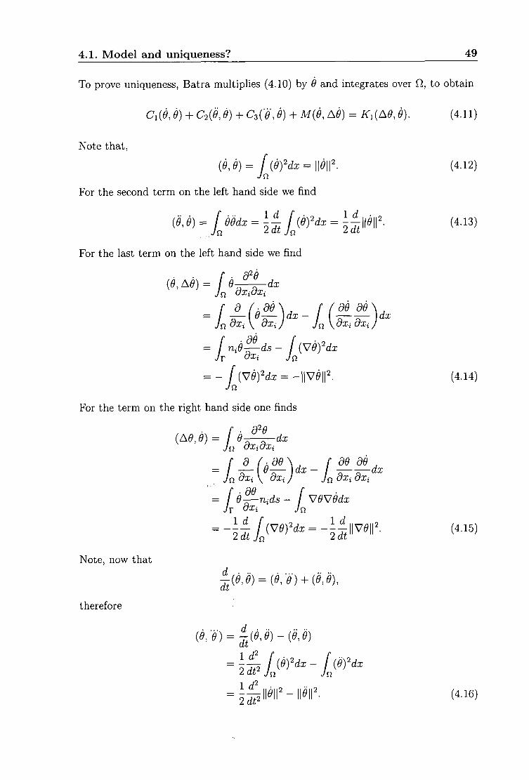
To prove uniqueness, Batra multiplies (4.10) by 9 and integrates over Q, to obtain
C,{9,9) + C2(9,9) + C^{9,9) + M{9, A9) = K,{A9,9). (4.11)
Note that,
{e,9) = / {9fdx=\\9\\\ (4.12) Jn
For the second term on the left hand side we find
( M ) = / ^ < ' < i x = i | / j . ) ^ . x = i ^ | M ^ (4.13)
For the last term on the left hand side we find
{9,M)= I 9 ^ ^ d x Jn /Q " dxidxi
Jn dxi V dxij Jn \dxidxij
= ~ ((\!efdx = - \ v e f . (4.14) Jn
For the term on the right hand side one finds
Jn axi \ dx, J JQ dxi dxi
= f 9^n,ds - / V9V9dx JT dXi Jn
Note, now that
therefore
f^{9,9) = i9,-9) + {9,9),
{9:9) = f^ie,9)-{9,9)
Id^ 2dt^
2df^
[ {9fdx - [ (9fdx Jn Jn
(4.16)
4.1. Model and uniqueness? 50
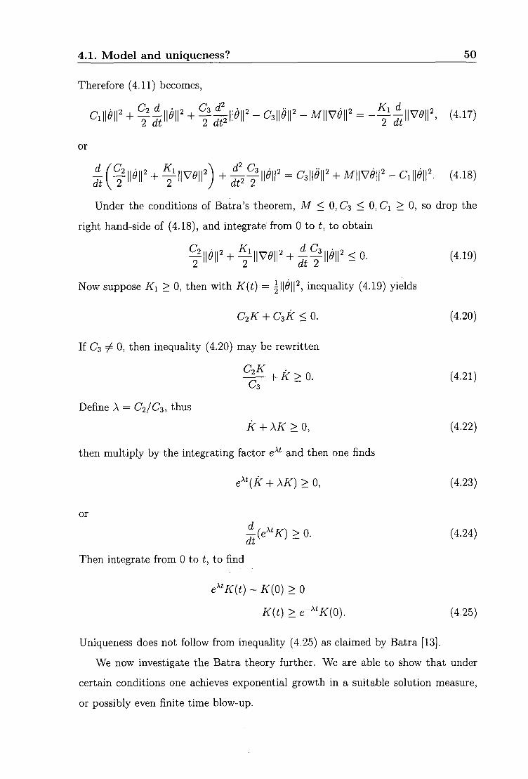
Therefore (4.11) becomes,
+ y + f ^ I I ^ I P - CsWer - MWWer = - ^ | | | V ^ I P , (4.17)
or
I (fll^ll^ + + ^ y l l ^ l P = 311 11 + M l i v ^ f - c m ' - (4.18)
Under the conditions of Batra's theorem, M < 0, C3 < 0, Ci > 0, so drop the
right hand-side of (4.18), and integrate from 0 to t, to obtain
Y N i ^ + ^ l W + | Y W < 0 . (4.19)
Now suppose Ki > 0, then with K{t) = inequahty (4.19) yields
C2K + Cjk < 0. (4.20)
If C3 7 0, then inequahty (4.20) may be rewritten
+ k>0. (4.21) C2K
C3 Define A = C2/C3, thus
k + XK>0, (4.22)
then multiply by the integrating factor e^*- and then one finds
e^\k + \K) > 0, (4.23)
or d ^ {e^'K) > 0. (4.24) dt
Then integrate from 0 to t, to find
e^'K{t) - K{0) > 0
K{t) > e-^'K{0). (4.25)
Uniqueness does not follow from inequality (4.25) as claimed by Batra [13].
We now investigate the Batra theory further. We are able to show that under
certain conditions one achieves exponential growth in a suitable solution measure,
or possibly even finite time blow-up.
4.2. Exponential growth 51
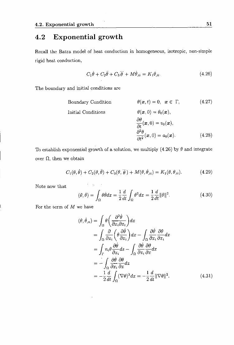
4.2 Exponential growth
Recall the Batra model of heat conduction in homogeneous, isotropic, non-simple
rigid heat conduction,
C,9 + C29 -H Ca' ' + M9^u = Ky9,u- (4.26)
The boundary and initial conditions are
Boundary Condition 9{x,t)=0, x E T, (4.27)
Initial Conditions 9{x,0) = 9 Q { X ) ,
39
— {x,0)=vo{x),
rP-9 | ^ ( x , 0 ) = ao(x). (4.28)
To estabUsh exponential growth of a solution, we multiply (4.26) by 9 and integrate
over Q, then we obtain
Ci{9,9) + C2{9,9) + C,{9, "9) + M{9,9^u) = K,{9,9,,). (4.29)
Note now that
For the term of M we have
d_ n dxi
9— dx- I ——dx oxi J dXi dxi
f ^39 ^ f 39 39^ = / ni9—ds- / ——dx
Jr 9xi Jn 3xi dx f d9_
Jn dxi 39 39 ^
dx . 3x
Id^ '2di
j j y ^ f d x = -\j^\\V9f. (4.31)

4.2. Exponential growth 52
For the term on the right hand side we obtain
IQ 8xi8xi {9,9,,) = [ 9 j ^ d x
Jn
= f f i e f ) , . - f ^^i. Jn dxi V oxij Jn 8xi8xi
= [ ni9^ds- [ dx Jr dxi JQ \8xiJ
Now, put (4.30), (4.31) and (4.32) in (4.29) to obtain.
\c^j^\m' + C,{9,9) + C,{9, -9) - f | l | V ^ f = - ^ i l l V ^ I I ^ (4.33)
Define ^ = {9,9), thus
d^ _ d ~dt ~ Jt
therefore
/ 99dx= I ^{99)dx Jn Jn
/ 9"9dx+ / Mdx Jn Jn
{9,9) + i^^^) = M ) + ~ J ^ i ^ ) ' d x
(^/6'') + ^ | l l ^ l P , (4.34)
{9,9) = '~§-lf^ll9r. (4.35)
Since ^ = {9,9), put (4.35) in (4.33), and we find
I c ^ l l ^ f . C . ^ . C a f - ^^11^11= - f IllWlP M = 0 (4.36)
Then, rearrange to obtain,
C 3 ^ + C 2 ^ + ^ , (^im' - ^ m ' - + \\v9r = o. (4.37)
dt dt \ A I I J
Divide (4.37) by C 3 0, thus (4.37) becomes . C2 ^ , d f Ci , ,^,2 1,,A | ,2 M ^^^a\^2\ , - ^ i IIV7£)H2
Put fj. = — C 2 / C 3 , then equation (4.38) may be rewritten,

4.2. Exponential growth 53
where G(t) = + ^ | | V ^ f - ^ f ^ n ^
Let ^ = - g - , then (4.39) is
Use an integrating factor
di
but
then
Put (4.43) in (4.41), therefore
dt\ J V /
and upon integration from 0 to t we find
= e-'^'G 0 Jo e->''i]xG + \\\/e\\^]ds, (4.45)
or
or, rearrangmg
e"' 'J? = e-^'G + f e-^' {]iG + ^\\^Qf\ ds + ^ ( 0 ) - G(0). Jo \ J
Let now Q{t) = ]xG + ^|| V6'|p, then (4.47) may be wriiten
e-^'^ = e-^'G + f e-^'Q{s)ds + ^.(0) - G(0). Jo
Divide (4.48) by e'^^ to obtain
^{t) = G{t) + f e^^'-'^Q{s)ds + e^\^{0) - G(0)). Jo
(4.40)
(4.41)
(4.42)
(4.43)
(4.44)
e-^^^^ - ^ ( 0 ) = e-^'G - G(0) + / e'^' fxG + ^\\V9\\^ ds, (4.46) Jo \ J
(4.47)
(4.48)
(4.49)

4.2. Exponential growth 54
Now recall that
= ^ 5 W I ^ - | * . (4.50)
In addition we define
K{0) = ^ ( 0 ) - G(0). (4.51)
Next, employ (4.50) and (4.51) in (4.49) to see that
- = G{t) + e^^'-^^Q{s)ds + e^'K{Q). (4.52)
Define now F{t) = \\9\\'^, then from (4.52) we have
I F " - \\9f = G{t) + f e^^'-'^Q{s)ds + e'^'KiO), (4.53) 2 Jo
or taking a term to the right hand side
F" |2 • — i i rz I
2 + G{t)+ f e''^'-'^Q{s)ds-he^'K{0), (4.54)
Jo
and then multiplying by 2 we arrive at
F" = 2\\9\\^ + 2G{t) + 2 f e^^'-'^Q{s)ds + 2e^'K{id). (4.55)
Next, substitute for G{t) in (4.55), to obtain
F" = 2\\9f + \\9\\^ + ^ l l ' v ^ l l ' - ^ l l ^ l l ' + 2 f e^^'-'^Q{s)ds + 2e^'K{<d), (4.56) (- 3 (^3 7o
or,
F" = 3 1 1 ^ 1 1 ' + ^ I IV^I I" - %\9f + 2 f e>'^'-'^Q{s)ds + 2e^'i^(0). (4.57) C/3 (^3 Jo
If M/C3 > 0, -C1/C3 > 0, Q{s) > 0, Vs > 0, thus (4.57) becomes
F" > 2e'''K{0). (4.58)
Recall Q{t) = iiG{t) + ^\\V9\\^
= f + f ^ l l V ^ I I ^ - ^\\e\\' + (4.59)

4.3. Explosive instability in a Batra model 55
where ^ = - C 2 / C 3 and E, — -K^/C^. Thus, if we suppose ^ > 0 and ^ > 0, then Q{t) > 0, as required.
Inequality (4.58) is the fundamental inequality from which exponential growth
follows.
Now, integrate inequality (4.58) from 0 to t, thus
F'{s)\l>^-^{en\l (4.60)
or
F'(t)>'^^^{e^'-1) + F'{0). (4.61)
Further, integrate (4.61) from 0 to t, to find
F{t) - F(0) > J\e''' - l)ds + F'{0)ds
\ f^J Jo
= H ( 2 ) ( f ! ! _ , _ i ) + 2 ( , „ , , „ ) , (4.62)
Rearrange inequality (4.62) to obtain
F{t) > F(0) + ( — - t - - ] + 2{e, d)ot
= F(o) + f 4(e'" - 1 ) - -1 ^ ( 0 ) + 2(^, e)ot
= l l ^o f + (\{e>^' - 1) - - ) ( ^ ( 0 ) - G(0)) + 2(^, e)ot.
Therefore
> IM' + {-Ae^' - 1) - ( ^ ( 0 ) - G(0)) + 2{d, 9)ot, (4.63)
Provided ,^{0) — G(0) > 0, since fx > 0, inequahty (4.63) leads to exponential
growth of \\e{t)f.
4.3 Explosive instability in a Batra model
We now investigate a generalization of equation (4.26) for which we are able to
establish that a solution ceases to exist in a finite time. A similar result for another

4.3. Explosive instability in a Batra model 56
third order in time equation was established by Quintanilla and Straughan [151 .
Recall that with M = K4 + C4 and K = A"i, equation (4.26) is
Ci9 + C2d + C39 + MM = KA9. (4.64)
We here suppose that K is a. function of temperature. This is realistic because in
general the thermal conductivity does depend on temperature. Thus, we consider
the following generalization to equation (4.64),
C^'e + C26 + Ci6 + MM = V(X(0)V0) . (4.65)
For our instability result we require either
C 3 > 0, C 2 < 0, Ci < 0, M > 0 and X < 0, (4.66)
or
C 3 < 0, C 2 > 0, Ci > 0, M < 0 and K >0. (4.67)
It is easy to see (4.66) and (4.67) are equivalent. Suppose now (4.66) holds. Then
divide by C 3 and we find 9 satisfies the equation
"9 -a9- a29 = -pA9 - \/{f{9)^9), (4.68)
where C2 M
a = , ^2 = (4.69)
and we have chosen
f{9) = -K{9) = l + a9', (4.70)
for a, e positive constants. We could easily have f = ko + a9^ for ko > 0 and our
proof will carry through.
Suppose ^ > 0, an assumption which is realistic given 9 is temperature. Then
9 satisfies equation (4.68) on the domain Q x (0, T) together with the boundary
condition
9{x,t) = 0, XET, (4.71)
and the initial conditions
89 9{x,0) = 9o{x), —{x,0)^vo{x),
— ( x , 0) = ao{x), xen. (4.72)
4.3. Explosive instability in a Batra model 57
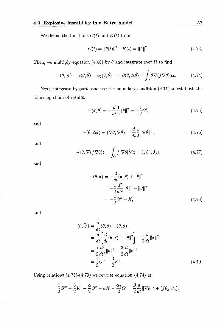
We define the functions G{t) and K{t) to be
G{t) = m t ) f , m = \\e\\ (4.73)
Then, we multiply equation (4.68) by 6 and integrate over fl to find
(9, "e) - a{9,6) - a2i9,9) = -p{9, A9) - f 9S7{fVe)dx. (4.74) Jn
Next, integrate by parts and use the boundary condition (4.71) to establish the
following chain of results.
d 1 1 ^ . (4.75)
and
and
and
-{9,A9) = {V9,V9) = j^l\m\',
- ( ^ , V ( / V ^ ) ) = / f\V9\'dx = { f e ^ i , 9 , ) , Jn
(4.76)
(4.77)
-{0,9) = --{9,9) + \\9r
(4.78)
and
{9,e) = j ^ { 9 , 9 ) - { 9 , 9 )
- 1 ~ dt
= 1 ^ ~ 2dt^
= 2^
ld_ 2dt
3_d 2dt
(4.79)
Using relations (4.75)-(4.79) we rewrite equation (4.74) as
M\f + {f9,,9,).

4.3. Explosive instability in a Batra model 58
We multiply by 2 and rearrange this equation to obtain
G'" - aG" = 2>K' - 2aK + ^{a^G + l3\\Vdf) + 2(/^,i,^,0- (4.80) at
Now, multiply by the integrating factor exp(—af) and write —2aK = —"iaK + aK,
and then from (4.80) one sees that
4[exp(-aO(:;"] = 3 ^ [ e x p ( - a O ^ ] + a^e- '^ '+ 4[e~"*(c^2G +/?||V^in] at at at
+ a e x p ( - Q i ) ( a 2 G + (5\\Vef) + 2 e x p ( - a i ) ( / ^ , „ ^ J . (4.81)
We integrate this equation from 0 to i and multiply the result by exp(Q:t) to arrive
at
G"{t) = ZK + a2G + (^WVeW + a f e''^'-'\K + a^G + (5\\Vdf)ds
Jo
+ 2 f e''^'-'\fd^u9,i)ds + Koe''^ (4.82) Jo
where the initial data term KQ given by
= G"(0) - 37^(0) - a 2 G ( 0 ) - /?||V^o||'. (4.83)
RecaUing the definitions of G and K in (4.73) and the initial data in (4.72), we find
Ko = 2(^0, ao) - U\? - oc2m? - PW^Oof. (4.84)
We henceforth require KQ > 0. (4.85)
This condition can always be achieved and requires the initial temperature and
temperature acceleration to be sufficiently different that (4.85) holds.
Next, we return to (4.82). Since a2,P,a and KQ are all non-negative we may
deduce from (4.82) that
G" >2 f exp[a{t - s)](/^,i, e ^ i ) d s . (4.86) Jo
Recall / = 1 + a r . Then
(/^,i ,6 ' , i)= / \V9\^dx + a f O'd^iO^x Jo. Jn
>a I O'e^iO^idx. (4.87) Jn
4.3. Explosive instability in a Batra model 59
Now, define
F{t)= [ G{s)ds. (4.88) Jo
Combine (4.87) and (4.88) in inequality (4.86) to find
F"'>2a Te^^'-^) / 9^9,^9^idxds. (4.89) Jo Jn ' '
To handle the right hand side of (4.89) we write
Jn
Xia (1 T7/2y
where Ai > 0 is the constant in Poincare's inequality | |V0|p > Ai||(;/!)|p for functions
0 which vanish on Q. Next, use Holder's inequality
/ 9^dx < ( / dxY^'^i f 9^Pdxy/^, - + - = 1. (4.91) Jn Jn Jn P Q
Pick
p = —-— and then q = .
Thus, with m denoting the volume of Q we find
\ 2/(2+£)
or rearrangmg, (2+e)/2
9^+'dx>-^( 9^dx] = - ^ - | | ^ | | 2 + ^ (4.92)
Thus, combining (4.92) and (4.90) one sees that
Now use (4.93) in inequality (4.89) to find
F'" > k f e""^'-'^\\9{s) f^'ds, (4.94) Jo
where

4.3. Explosive instability in a Batra model 60
We must now estimate the right hand side of inequality (4.94) in terms of F. To
do this we again employ Holder's inequality as follows, where ^ > 0 is a constant to
be chosen.
Jo Jo
< 1/9 / H
Wer^d^ (4.96)
Pick 2+e , 2+e
p - —-—, whence q =
and from the inequality above one derives
rt / ft / ll^ll^ds < / exp
Jo \Jo
(r X / exp
\Jo Now, choose ^ = 2/(2 + e), then
Jo I Jo
.Jo
- a^t - s)
Hit - s)
(2 + £) 6
2 + e
ds e/(2+£)
2+e ds 2/(2+£)
(4.97)
2/(2+£) / /.t
/ JO
exp a-{t - s)
2/(2+e) / f t \
ds
e/{2+e)
e/(2+£)
e 2^
^/(2+£) 1 — exp
-2(xt e/[2+e) y ft x 2/(2+6)
\Jo J
We now bound the second term on the right by 1 to find e/[2+e ft / \ £/i^+£; r ft 2/{2+£)
£/2
Thus, rearranging (4.99) yields
re"(*-)p(5)| |2-^^d5> {—] F(2+^)/2. Jo \ ^ J
Finally, use of (4.100) in inequality (4.94) shows
F'" > kF^+''\ where k = k{2a/ey''.
(4.98)
(4.99)
(4.100)
(4.101)
To show (4.101) leads to global non existence of a solution suppose OQ ^ 0, then
F'(0) = pQf > 0. Multiply (4.101) by F ' to show
2k \ d {F'F'y > [F"f +
A + e dt _p2+e/2 (4.102)
4.4. Thermal discontinuity waves in the Batra theory 61
Integrate this inequality from 0 to t to obtain
F'F" > F'(0)F"(0) + ( — ) F^+'/\ (4.103) \ 4 + £ /
Now multiply this inequality by F', integrate from 0 to t and multiply the result by
3. One finds
{F'f > [F'{0)]' + 3F'(0)F"(0)F(i) + -fF^+'/\ (4.104)
where the constant 7 is given by
_ 12fc ^ " (4 + e)(6 + e) •
The proof now proceeds by contradiction. Suppose 6 exists for all time t > 0.
Then
F'>{a, + P,F + ^F'+^/Y^
a i = [F ' (0)f , /3i = 3F'(0)F"(0), and so
The left hand side is bounded above by the analogous integral from F(0) to 00 and
then
t<n, (4.106)
where /•°° dF
^ " ^ i o ( a i + A F + 7 F ^ W 2 ) i / 3 ' (4.107)
where we have noted F(0) = 0.
Since < 00, inequality (4.105) shows t must be bounded which contradicts
the fact that 9 exists for all time t > 0. In fact, 6 cannot exist globally beyond the
value t — Tu-
The expected behaviour of 9 is that it blows-up in a finite time T > T^.
4.4 Thermal discontinuity waves in the Batra the
ory
Batra [13] found the wavespeed of a discontinuity wave in the linear version of his
theory. We now analyse discontinuity waves in his model, but for the fully nonlinear

4.4. Thermal discontinuity waves in the Batra theory 62
theory. A further study of thermal waves in a rigid heat conductor is contained in Chapter 5.
Recall the complete equation of Batra [13], with the heat supply r = 0,
In this section we restrict attention to a one-dimensional discontinuity wave. Thus,
e and q are functions of the variables
e, e, e, 0,, 4 , 0 , , (4.109)
Using (4.109) in (4.108) and expanding we see that
600 + Egd + Eg 9 + seX + ^ej^ + ^e.Jxx
+ qe9x + + QeOx + Qejxx + Qejxx + Qe.Jxxx = 0. (4.110)
A discontinuity wave for (4.110) is a singular surface, analogous to an acceleration
wave, S, across which 9,9x,9xx and 9xxx possess a finite discontinuity. The higher
derivatives may also be discontinuous across S. However, ^ G C" in both x and t.
As stated in the introduction the jump of a quantity / is
[/] = r-r where
f^= Urn f{x,t). I—>s*
Taking the jump of equation (4.110) and recaUing the regularity properties of S, we
obtain
^elO] + ^eM + ee,A9xx] + qg[9x] + <79.fex] + Qe.AOxxx] = 0. (4.111)
The Hadamard relation is
^-^ = [ft] + V[U (4.112)
where 5/5t is the derivative of a function at the wave S, as seen by an observer on the
wave, and V is the speed of the wave moving in the x-direction. Since ^ G C^(M x R)
we find the chain of relations
TM = 0={9]+V[9XI (4.113) dt

4.4. Thermal discontinuity waves in the Batra theory 63
and
Y^%] = 0=[9,] + V[9,,i (4.114)
and
^ W = 0 = [ 4 x ] + \^[^xxx]. (4.115)
From (4.113)-(4.115) we derive
[9] = -V[9:,] = V'[9,,] = -V'[9,,,l (4.116)
[^x] = - V [ 4 x ] = (4.117)
and
[ 4 x ] = - l ^ [ ^ x x x ] - (4.118)
Next, use (4.116)-(4.118) in equation (4.111) to find
[9..A{-V'e^ + - V^0.J + [dr.r]{V'Qe - VQe. + <le..) = 0. (4.119)
We require that [^m] ^ 0, otherwise we do not have a discontinuity wave, and then
equation (4.119) yields the following equation for the wavespeed V,
- V\e,^ + q^) + V{ee^^ + q j - qe^^ = 0. (4.120)
This is thus a cubic equation for V. In general we shall find three solutions for V.
To make a comparison with the work of Batra [13] (who only studied discontinuity
waves in the hnear theory) we suppose the wave, 5, is moving into an equilibrium
region for which 9'^ = constant and so 9^ = 0, 9^^ = 0,9^ = 0, 9+ = 0. In this case
dq 39
= 0, E ^^x 39.
= 0. (4.121) E
Equations (4.121) follow since by the representation we must have for (jj and e in the
three dimensional theory, terms Hke dqi/d9 will involve 9^i, etc, and so dqi/d9\E = 0 .
For a wave moving into equilibrium, equation (4.120) reduces to
V{s^V' + Ee^^+qeJ = 0. (4.122)
Equation (4.122) has solution
y = 0, \ / = ± J - ^ ^ ^ i ^ , (4.123)

4.4. Thermal discontinuity waves in the Batra theory 64
Solutions (4.123) correspond to those of Batra [13], his equation (4.7) when we adopt a linear theory and the appropriate expressions for q and e. Of course, our equations (4.123) are valid for a general nonlinear theory. The only solutions of interest are
y (4.124)
Since physically we must have V'^ > 0, this imposes the restriction on the derivatives
of q and £, in the sense that we must have
'-hl±SL^O. (4.125)
Equation (4.125) imposes a restriction on the possible forms of nonlinear functions
e and q may have.

Chapter 5
Thermal waves in a rigid heat
conductor
This work is published in Jaisaardsuetrong and Straughan [81]. There has been a
huge amount of interest in theories which allow heat to propagate as a wave. For
example, extensive reviews of Chandrasekharaiah [22] and Hetnarsky & IgnaczaJt [69
study several thermal wave theories coupled to the equations of elasticity. There
are many theories which allow heat to propagate as a thermal wave and among
these we quote the theories of Green & Laws [58] where a generalised temperature
(p{T,t), T being absolute temperature, is introduced, the two temperature theory
of Chen k Gurtin [25], the history-dependent theory of Gurtin k Pipkin [67], the
dual phase lag theory of Tzou [183], the t theory of Cattaneo [19], and its extension
to thermoelasticity by Lord & Shulman [109], and the internal variable theory used
by Caviglia et al. [20]. We note that the theory of [9] in the linear case reduces to
that of Lord & Shulman [109], as connectly observed by Chandrasekharaiah [22 .
A more recent theory which allows heat to propagate as thermal wave is intro
duced by Green & Naghdi [60] whose thermodynamics employs an entropy balance
equation, rather than an entropy inequality, and a thermal displacement variable
a ( x , 0 = rr (x ,s )ds . (5.1) Jto
In equation (5.1) the temperature field T is defined by Green & Naghdi [60] to be
an empirical temperature. This temperature is, however, equivalent to the absolute
65

Chapter 5. Thermal waves in a rigid heat conductor 66
temperature as shown by Green & Naghdi [ [64], pp. 338-340]. The theory of Green & Naghdi [60] has been extended to thermoelasticity and many applications are reviewed in [1] and [2], mainly in a linear setting. The theory of Green & Naghdi [60 relies on a variable 9 which they call a temperature, although it is actually a function of a and T, so that 6 — 9{ct,T) = 9{a,a). While there may appear some formal similarity with the Green & Laws [58] theory where (p = (l){T, T) the two theories are very different. In fact, most applications to date of the Green h Naghdi [60 theory assume a particular form and work with a rather than 9. In this work the goal is to analyse the ful l nonlinear theory of Green & Naghdi [60], the theory they refer to as type I I , for a rigid body, and we keep 9 = 9{a,T). We have not seen any study like this before. (It is worth pointing out that both type I and type I I I heat conduction in a rigid body lead to nonlinear theories, see Green & Naghdi [60], but wave motion in these theories is very different.) We maintain that which of the many heat propagation theories will be useful in a mundane situation will depend on an extensive and rigorous analysis of each theory and the aim in this chapter is in this fine.
There are many recent applications of the various theories outlined above, to
a variety of problems, mostly in a hnear context. While these are too numerous
to list we do draw attention to the paper of Jordan & Puri [94] where they make
a very useful comparison of the Lord & Shulman [109] model and the Green k
Laws [58] model with that of classical Fourier theory. Christov &; Jordan [26] analyse
the Cattaneo theory as do Pranchi & Straughan [51], who also dwell on the fact
that a constant relaxation time r in the Cattaneo theory is not consistent with
thermodynamics. Puri & Jordan [139] and Quintanilla & Straughan [152] study
wave motion in thermoelastic bodies of type I I I . The Tzou [183] (third order) theory
is studied from various angles by Quintanilla k Racke [147], Quintanilla [144] , Jou
and Criado-Sancho[19], and Serdyukov[20], while Quintanilla & Straughan [151]
show that finite time blow up is possible with third order theory when the thermal
conductivity is a nonlinear function of temperature, as it often is in practice. Puri
& Jordan [140] analyse the two temperature theory of Gurtin & Pipkin [25] in some
depth. Many other recent references may be found in these chapter.
5.1. Basic equations and thermodynamic restrictions 67
The goal is to perform a complete analysis of acceleration wave motion in a Green & Naghdi [60] rigid solid of type I I . By a rigid body we follow the definition of Green & Naghdi [ [60], p. 177] and such a body is one for which the distance between any two particles remains unchanged whatever the motion maybe. We keep the equations of [10] in their full generality, ful l nonlinearity, and we completely determine the wavespeed and the amplitude of the wave as a function of time. While the mathematics behind acceleration waves, cf. Chen [24], has been around for some time, the fact that its use reveals very useful understanding of the physics of a problem justifies its use. In this regard we cite the recent papers of Jordan & Puri [92,93], Jordan [86], Christov et al. [27], Pu & Scott [55], Quintanilla & Straughan [152] where acceleration waves are employed, and many other articles dealing with acceleration waves are cited there.
5.1 Basic equations and thermodynamic restric
tions
The fundamental equation of Green & Naghdi [60] is the balance of entropy, equation
(7.20a), which is
PV = P( + PS - Pi.i, (5-2)
where rj, ^, s and Pi are, respectively, density, entropy, internal rate of production
of entropy per unit mass, external rate of production of entropy per unit mass, and
the entropy fiux vector. Standard notation is used throughout, so a superposed
dot denotes d/dt, subscript comma i denotes d/dxi, and repeated indices denote
summation from 1 to 3.
Fundamental theory are a temperature function 9 = 9{T, a) such that ^ > 0 and
d9/dT > 0. In addition. Green & Naghdi [ [60], pl85], show how the energy balance
equation may be exploited to deduce restrictions on the thermodynamic variables
which may be interpreted as defining 77, pi and ^ in terms of a Helmholtz free energy
function ip — il>{9,Pi)- The relevant relations follow from Green & Naghdi [60],
5.1. Basic equations and thermodynamic restrictions 68
equation (8.15), and are
^ ~^W^df' ^^^^^ ^ ^ ^ ^ ^^"^^
f = 2 A V ' . ^ + ^ ( 5 ? | ^ - ^ . ) , (5.5)
A = a,ai = AA, (5.6)
and we write e.g. '0a = dip/dA.
For our analysis there is no less in generality in setting the external supply of
entropy to be zero and so we henceforth assume s = 0. Then, using (5.3)-(5.6),
equation (5.2) may be written as
where we have defined
Aia,a,a,) = A='^ and / i i = (5.8)
The above equations represent the general theory of heat flow in a type I I rigid
body of Green k Naghdi [60]. However, we may wish to consider the following
special cases,
i^ = c[9- 9\n9) + ^AA (5.9)
and
= c{9 -9\xi9)^^(3i(3i, 9 = a + bT (5.10)
c, k, a, b positive constants, where c and k denote the specific heat and heat con
ductivity. Case (5.10) is considered by Green k Naghdi [60]. Note that, in these
cases the theory is still nonlinear. Moreover, from equation (8.15)4 of Green k
Naghdi [60], for case (10), ^ = 0.
While we concentrate on a rigid heat conductor of type I I , we point out that
Green k Naghdi [ [60], pp.183-188] also define such a heat conductor in type I or
type I I I cases. Very briefly,, the key difference is the list of independent constitutive
variables. This list comprises T and Ti for type I ,T, o; and a,, for type I I , and
T, Q:, T I and a,, for type I I I . Type I I leads to a very different equation to both type
I and I I I , the latter types both containing substantial damping.
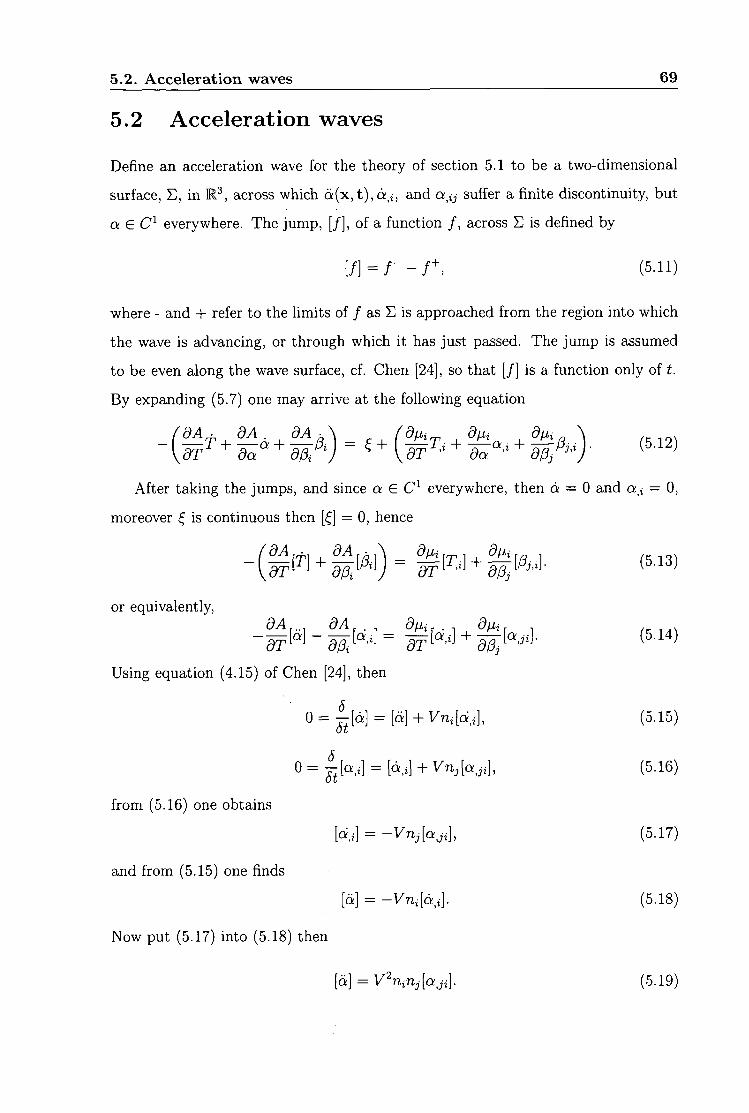
5.2. Acceleration waves 69
5.2 Acceleration waves
Define an acceleration wave for the theory of section 5.1 to be a two-dimensional
surface, E, in R^, across which Q:(x, t) ,a , j , and a,jj suffer a finite discontinuity, but
a e everywhere. The jump, [ / ] , of a function / , across E is defined by
[ f ] = r - r , (5.11)
where - and + refer to the limits of / as E is approached from the region into which
the wave is advancing, or through which it has just passed. The jump is assumed
to be even along the wave surface, cf. Chen [24], so that [/] is a function only of t.
By expanding (5.7) one may arrive at the following equation
OA. dA dA.\ f d f i , di,i ^ 5 / . , \
After taking the jumps, and since a e everywhere, then o; = 0 and a,i = 0,
moreover ^ is continuous then [^] = 0, hence
or equivalently. dA dA dfii df^r
Using equation (4.15) of Chen [24], then
0 = Tila] = [a] + Vuildi], (5.15) dt
Q = j-^[ai\ = [a^] + Vn,[aJ,], (5.16)
from (5.16) one obtains
d_i] = —Vnj[aji], (5-17)
and from (5.15) one finds
ci] = -Vmla^i]. (5.18)
Now put (5.17) into (5.18) then
a] = V^niUjlaji]. (5.19)
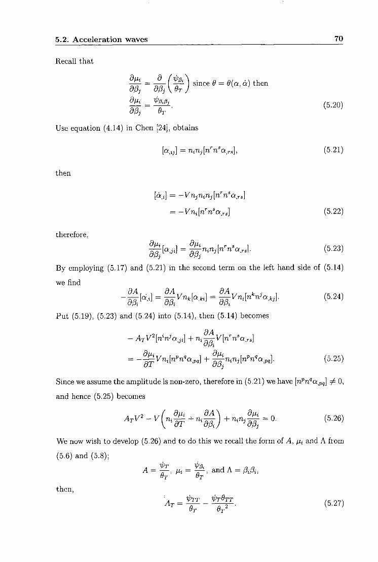
5.2. Acceleration waves 70
Recall that
dm ^ d f
dpj 9T •
Use equation (4.14) in Chen [24], obtains
(5.20)
a^ij] = riinjlrin^a^rs], (5.21)
then
[ci,t] = —Vnjriinjln^n^a^rs.
= -Vni[n'n'ars] (5.22)
therefore,
= ^n^nAn^n^arsl (5.23)
By employing (5.17) and (5.21) in the second term on the left hand side of (5.14)
we find
- — a,i = -^Vukla^ki] = ^Vni[n''n^akj]- (5.24) dPi aPi oPi
Put (5.19), (5.23) and (5.24) into (5.14), then (5.14) becomes
dA - ArV^ln'ri^aji] + ni—V[n''n^a^rs,
(jPi
= -^Vn,[n^n^a,,] + | |n ,n , [n^n^a,p , ] . (5.25)
Since we assume the amplitude is non-zero, therefore in (5.21) we have [mFn'^a^p,] ^ 0,
and hence (5.25) becomes
^ , ^ . _ ^ ( „ . | ; , „ , ^ ) ^ ^ „ , | i = 0 (5.26)
We now wish to develop (5.26) and to do this we recall the form of A, ^ and A from
(5.6) and (5.8);
A = ^ , ^ , = | ^ , a n d A = A/?.,
then,
9T 9' ^ r = ^ - ^ . (5.27)
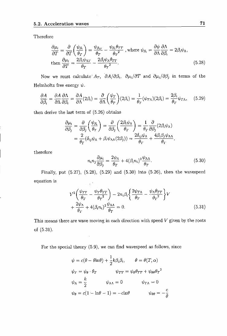
5.2. Acceleration waves 71
Therefore
diii d f ^pA ^PiT ^Pi^TT , , di^ dA
' ^ ' ^ 5 r = ( ' - ' ^ ^
Now we must calculate 'yl^, dA/dPi, djii/dT and dfii/dPj in terms of the
Helmholtz free energy ip-
then derive the last term of (5.26) obtains
din d d / 2 A ^ A \ _ 1 d
dPj d p A e r ) dp A OT J erdP: {2PM
2 /X / , /? / /o/Q ^ '^^ij'^A , iPiPji^AA
therefore
Finally, put (5.27), (5.28), (5.29) and (5.30) into (5.26), then the wavespeed
equation is
,2 f ^TT _ IPTOTT\ _ 2 n p ! ^^^^ - ^^^^^
+ ^ + 4 { f t n 0 ^ f ^ = 0. (5.31)
This means there are wave moving in each direction w i t h speed V given by the roots
of (5.31).
For the special theory (5.9), we can f ind wavespeed as follows, since
iP = c{9- e\ne) + ^kPiPi, 9 = 9{T, q)
k i>A= 2 ^ ^ ^"^^ ^ ^
i;e = c[\ - \ n 9 - l ) =-dn9 ^00 = -^

5.3. Homogeneous region 72
put these equations into (5.31), then the wavespeed equation reduces to
rearrange to obtains
^ - r ' " " - ' - - - ^ - 2 n A [ - l " ^ V ) ^ f - . (5.32)
OT "T
ox equivalently,
^-^\kn.0f-^V^^ = ^^ (5.33) u Cj. 177
For the case (5.10), as follows,
^ = c{e -e\nd) + ^^i(3i, d = a + bT,
equation (5.31) reduces further by
Ox = b, 9TT — 0,
then the wave speed theory for case (5.10) is
f rom which i t is clearly seen there are waves moving in opposite directions w i t h
speeds V = ±b-^y/ke/c.
5.3 Homogeneous region
We can calculate the wave amplitude
a{t) = [a], (5.35)
exactly, even in the general case studied in section 5.2. However, the key physics is
perhaps easier to see by considering a wave moving into a homogeneous region for
which
a,i - A = 0. (5.36)
We henceforth restrict attention to this situation.

5.4. Amplitude behaviour 73
For the wavespeed we find equation (5.31) reduces to
^ ' = 2 V ' A / ( ^ - ' / ' T ^ ) - (5-37)
Under the same conditions, equation (5.33) becomes
while equation (5.34) remains the same.
5.4 Amplitude behaviour
To calculate the wave amplitude a{t) = [a] one expand (5.7),
-{ATOC + A^a + A^A) = C(a, T, A ) + ^ d , , + ^ a , + |^/?,,.
Then differentiate w i th respect to t,
- ( ^ A A + K{AATa + A^aa + ^ I A A A } ) = ^ ^ d + ^ r d + CAA
Recalling that
A = PiPi =
A = 2pi$i = 2a,id,i
A = 2{Q! , id i + d , id , i} ,

5.4. Amplitude behaviour 74
then (5.39) becomes,
- {ATTOC'^ + AraCiOi + ATAa{2a^id^i) + Aroi) - {AarOia + AaaCxct + AaA2aa^id^i + Aad)
- AAr(i(2a, i ( i , i ) + AAaa(2a,iCt,i) + /lAA(4a,iQ,ia,fcd,fc) + AA2{Q,ia i + Q,ia,i}
= '^aa + '^Ta + ^ A ( 2 a i a i )
5/3^ aaa/5j '- a r a / j j oPkdPj
Take the jumps of the resulting equation w i t h take into account that the wave
is moving into a homogeneous region, a^i = 0 and since ct G C \ then this becomes,
- ( ^ r r M + >lTQ[ci]a + Arid]) - {Ac,Td[d] + Aa[d]) + 2AA[d^id^i
a/?j dadaj dTdPj dPkdPj Recall
^. = tiL = —IPJ^— = —2(3-9T OT dPi OT
Define denotes the homogeneous region, therefore in the homogeneous region
we have
lJiiaT\E = 2 ( 5 i { ^ = 0 , (5.40)
also.
Furthermore,
^J'iTPj\E _d_
dp,
I^^TT\E = 2a4'^) = 0 . (5.41)
and so,
2 4 « ( ^ ) ^ , (5-42)
|^U = 2 f t ( | ) , = 0, (5^43)

5.4. Amplitude behaviour 75
similarly.
and,
Moreover,
a y . a/5,a/?,-
Also,
Hence the am
= 4 ( ^ ) ^ ( A ^ , f e + M O - o .
iplitude equation becomes,
(5.44)
(5.45)
(5.46)
- A r x [ d ] ^ - 2ATaT[6i\ - AT[oi] - Aa[Q\ - 2ylA[d,id,j
= ^ r [ d ] + 2 — < [a,id,i] + [aa^a] \
^ i r i ' t f ) l a , . ) + 2 ^ 1 6 . . ] ^ (5.47)
The Hadamard relation or condition of kinematical compatibility, see Chen [24], is
5 5t [ f ] = [ft] + Vn,[f,i] (5.48)
where 5/5t is the derivative of a function on the wave as seen by the observer on the
wave. We now use (5.48) and the wave speed equation to remove the [d ] and [a^u
terms, therefore
(5.49) — [d] = [d ] + K[n 'd ; , ] ,
^ [ d , i ] = [ d j ] + Vnj[a\ij], (5.50)
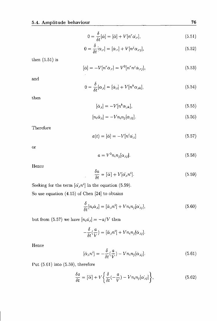
5.4. Amplitude behaviour 76
0= ha] = [a] + V[n'dr], (5.51) ot
0 = j-^[ar] = [ar] + V[n^arj], (5.52)
then (5.51) is
and
then
Therefore
or
Hence
5t
Seeking for the term [d'in^] in the equation (5.59)
So use equation (4.15) of Chen [24] to obtains
a] = -V[n'a,r] = V^[n^n^a,rj], (5.53)
0 = ^ k i ] = k i ] + V'[nVffc]> (5.54)
a,i] = -V[n''a^ik], (5.55)
rijd^i] = —yniUjla^ij]. (5.56)
a{t) = [a] = -V[n'd,i] (5.57)
a = V'^niUjla^ij]. (5.58)
^ = [Q] + y [ a y ] . (5.59)
^ [ n j d j ] = [a,in'] + Vninj[Q\ij], (5.60)
but f rom (5.57) we have [riid^i] — —a/V then
- ^ ( ^ ) = [ a i ^ ' l + VniUjid^ij .
Hence
= - ^ ( ^ ) - Vriinj[a,j]. (5.61)
Put (5.61) into (5.59), therefore
^ = [ - l + v | ^ ( - - ) - V „ < n , [ c , . , ) | , (5.62)

5.4. Amplitude behaviour 77
smce \/-^ ( ^ \ — a SV
6i \ v ) " ~~5t'^V~5t'
then (5.62) becomes
Therefore
6a ...... 6a a 6a r . i /,-
T r 9 r 1 ^6a a 5V y n . n , M = - 2 - + [a ] + - -
l ' ' M = - 2 j ^ + l « l + ^ ^ . (5.64)
Now, we can obtain the term [a^a] as follows
Put (5.65) into the last term of the amphtude equation (5.47), therefore,
- Arr[ci:]^ - 2ATaT[a] - Aria] - Aa[a] - 2AA[a^ia^i
= ^r[ci] + 2 ( ^ ^ ) ^ | [ d , a i ] + [ a a , i ] |
f ^ A \ r . - A f 6a , , a6V]
B y rearranging,
- Arrlaf - 2ATaT[a] - A^[a] - 2AA[a,id,i] - Arl'a] - 2 - ^ [ a ] V ^Ut
= eT[a] + 2 f ^ ) / [ a , d , ] + [ d a i i ] } + 2 T f ^ ) [a^,] / L J \ 9 t J a
, o VA f a 5 V \
or simplicity.
- / lTT[ci ] ' - 2 X r a T [ f i ] - A^[a] - 2AA[a^a,,] + {-At - | ^ ) [ « ]

5.4. Amplitude behaviour 78
Recall that the wavespeed relation in homogeneous region (5.37) is
T/2 o / I (i^rOxT , ^ = 2'ipA / ^ - ^ t t J .
or V^At + 2 ^ ^ = 0,
or At + 2 ^ = 0, (5.68)
therefore this term has been vanished in (5.67), hence the amplitude equation be
comes
- AtW - 2ATaTa - Aaa - 2AA[d^id^i] = + 2 ( ^ ) ^ + [<ia,u]^
+ 2 r ( | ) M + 2 ^ ( - 2 - + - - ) . (5.69)
Since the formula for the jump of a product that has been discussed by Lindsay
& Straughan [104]: [fg] = f~^[g] + g^[f] + [f][g], therefore
d^id^i] = 2d,i"^[a,i] + [d,i][a",j] = [d,i][d,j] , (5.70)
the term 2Q:+[Q;,i] of (5.70) vanished since the wave is moving ahead of the region,
d / = 0.
Prom (5.51) obtains
then,
rr -1 [< ] ^
9
i K i J 17 , hence [ a = ^7^ = F , i » i J , y ' L " , ' J L " , H y l
and f rom (5.58) we have ^^[a^ii] = a, therefore [ot^u] = a/V^, moreover
/ \ 2
= [d][au] = {a)i^^j (5.71)
Henceforth (5.69) can be reduced further as follows.
- Atto^ - 2ATaTa - Aaa - 2 A A y 2
- era + 4 ( - ) ^ ( - ) + - ( ^ - J ^ a + ^ ( ^ - ^ - 2 - j . (5.72)

5.4. Amplitude behaviour 79
Mul t ip ly both sides of (5.72) by V'^'BtI'^-^k, then obtains
By rearranging (5.73) obtains,
2 ^ + a / - l ? ^ _ ^ ' ^ ^ ^ ^ ^ ' ' ^ ' ^ ^ ^ ^ V-^^r^r T O r f ^ , '5t \ V 6t 2^A 2i/'A V^r
• ' ' ' - ^ + ^ + 2 ^ ( | ^ ) , V ^ = 0 . (5.74) 2^A ^ A ^^aOt^^J
Now the Maxwell relation and the wave speed equation are employed to remove
the [d] and [d^u] terms and we arrive at the amplitude equation
2 ^ + u;a - Ca = 0, (5.75)
where S/5t is the derivative of funct ion on the wave as seen by an observer on the
wave.
The coefficients LU and C are given by
V 5t ^ A KOrJTa 2^A V ^ T A V^T
v e r i f y . , , frr.i^T0a\ fr.^, 2 . A l V ^ ^ ^ ^ ^ J / r a . - l " f , .
' V 5 t ~ ^ A [oTjTa SV'A
V^erU^^_^) \ ( , 7 6 ) 2^A IV OOt Jr V 0 /TJ
We observe the effect of ^ is manifest in the last term of (5.76), the one involving
the braces:
= ^ r ^ J ^ " — tpa in equihbrium region. (5.78) 6 \ Ot J

5.4. Amplitude behaviour 80
The general solution to (5.75) is easily found, cf. Chen [24] as follows.
2— + w a - Ca = 0,
+ aa — f5o? = 0, where a = ^ and /5 = ^ , ot 2 2
— + aa = pa\
1 Sa a 6t a
Let / = - then
^-^-af = -p. (5.79)
Use integrating factor fj,{t) = e~- o "('^)'^'^, therefore (5.79) becomes
^ ( / / / ) = - p f i ,
MO/W = - f P{rMT)dT + f,{0)fiO),
smce
thus (5.80) becomes
a{t) =
a{ty
smce
therefore
^(0) = e- /o"W' i^ = l ,
g-/o'a(r)<ir
x(0)
However, its interpretation is perhaps easier seen by considering the special theories
(5.9) and (5.10).
For (5.9), we have
V; = c(^ - ein^) + ^ A , e^9{T,a),

5.4. Amplitude behaviour 81
then
0A = 2
i / , ^ = ^jj^Or = c ( l - \n9 - 1)9t = - c l n ^ • 9t.
ipa = tPeOa = c{l-\n9- 1)9^ = -cln9 • 9^
Hence, in this case,
and f rom (5.37) we have
1/2 _ M l ~ c9V
so C for special case (5.9) is
then.
C = - — ( l n ^ ) r T - - 7 — = - 7 - U - ^ T ' t / j - (77- (7J' y (7 J J. UT
9t n^TT C = y - 3 ^ . (5.81)
and,
u; = ^ ( - c l n ^ ) r a ^ ( - c l n ^ ) a
k ^9t''^ k W99t)t \ 0 \ 9 k9 1
Put V'^ = — — t h e n the term u can be rewritten as c 9^
1 5V 2T^r k9 . ^ ^ c9t k9 T^Ta " = - V - — + - ^
- ^ ^ ^ 4 - 2 ^ ^ 1 n e i 4- % l n ^ l
9Akf 9c.\ _^29 /^\n9 • 9^
c9T\99TJr 9 t \ 0 ;^
Since the wave is moving into the homogeneous region, a^i = 0, then
16V 2T9^ , 0 9Ta 29 \n9.9
The effect of is due to the last term of (5.82).

5.4. Amplitude behaviour 82
Finally, in case (5.10), we further assume T'^= constant, i.e. the temperature ahead of the wave is constant, thus
e = a + bT, eT = b, BTT = 0
kO then = — = constant, since 9 = a-\-bT = constant.
hence
so equation (5.75) becomes
1
u; = 0, C = — r ; ^ , (5-83) a + bl
| 4 „ ^ = 0. (5.S4)
+ a(t) • a i 5 ) = i i « ^ ) ' ' ^ _
Therefore solution is
Since C > 0, we see that if a(0) > 0 then a{t) blows up in a finite time to, where to
has derived f rom
Jo 2
b , 2 -as =
Jo a + bT^" a{0)' bt _ 2
a + bT ~ a (0) ' 2(a + bT+)
Thus, to depends on T in the homogeneous region. In the last case we have = 0 and
i t is interesting to note that this may always lead to the thermal shock formation.
For a deeper discussion of how an acceleration wave may develop into a shock wave,

5.4. Amplitude behaviour 83
see Fu & Scott [55]. To interpret thermal shock formation we note that the aid of Hadamard relation,
[a] = -V[a:,] = -V[T,]. (5.87)
Since = constant we may deduce T + = 0 and hence [a] = —VT~. The con
di t ion a(0) > 0 then implies T~ < 0 and f rom (5.85) T~ increases in absolute
value as time increases. Thus, as the wave moves right the temperature gradient
increases(negatively) and blow-up is consistent w i t h the thermal shock formation,
i.e. a j u m p in T (or 6*).

Chapter 6
Green-Naghdi theory for a fluid
We now consider a generaUzation of the theory of chapter 5, that developed by
Green and Naghdi [60 .
Green and Naghdi [65] extended their theory of [60] to be applicable to a perfect
fluid. They, however, adopted a special relation for the Helmholtz free energy of
fo rm
-0 = - m a , i a , i + / ( p , ^ ) , (6.1)
where m is a constant. A general theory satisfying the laws of continuum ther
modynamics was constructed by Quintanilla and Straughan [155]. Quintanilla and
Straughan [155] also developed a fu l ly nonlinear acceleration wave analysis w i t h a
very general form for —' 'lp{p, 9, V a ) .
In this section we derive the wavespeeds of an acceleration wave when the
Helmholtz free energy is more general than (6.1), but less general than that proposed
by Quintanil la and Straughan [155]. We assume that
i; = ^m{p,9)\Va\' + F{p,9). (6.2)
Here, m and F are allowed to be functions of p and 9. Note that again a is a
temperature displacement function,
a= f 9ds, (6.3) Jo
while p is the density.
84

Chapter 6. Green-Naghdi theory for a fluid. 85
The equations of Quintanil la and Straughan [155] are those of continuity of mass, the momentum equation, and the energy balance law, namely,
Pt + Vip^i + pvi^i = 0, (6.4)
1 d
p{vi^t + V j V i j ) = - - — {p{ipajOi,i + i p c i a j ) } , (6.5)
-p{^e,t + Vitpe^i) = {pipa,i),i, (6.6)
where the pressure p is given by
We note that f rom (6.2),
p = p 2 ^ , . (6.7)
-ipe-\m0\Va\^ + Fg, (6.8)
= ma , i , (6.9)
1 2
m,\ya\' + F„ (6.10)
i>ajOL,i + i>oi,i(^j = 2mQja , i . (6-11)
Employing the above relations, equations (6.4)-(6.6) become
Pt + Vip^i + pVi^i - 0,
p{vi,t + VjVi^j) = - p , i - {pma^iaj)j,
~'^{ Wt^^ " [pma^^^^. (6.12)
We now analyse the behaviour of an acceleration wave 5 for equations (6.12). By
an acceleration wave we here mean a surface <S across which a^, a^u, ^ i j , "i^i.t, P,t, P,i
and higher derivatives posses a finite discontinuity, but a £ C^(M'^), Vi,p G C°(M'^).
Equations (6.12) are expanded recalhng p = p'^ipp and •0 = tp{p,9,a^i) to find
after taking the j ump [ . ] across S,
Pt] + Vi[pA + p[viA = 0, (6.13)
PiM + = -Pe[9,i] - PPIPA - PaA^Ji] - - P'>^p[P,j](^,i(^,j
- pmg[9j]aja^i - pmaj{a^^j] - pma^a^jj], (6.14)

Chapter 6. Green-Naghdi theory for a fluid. 86
- Vipi^]^mee[0,i\a^rOc^r + ^mep[p,i]a,ra:,r + rneaj[aji\ + Fee[0,i\ + fflp[p,i]|
= /9,i]ma,i + pa^^{mg[6^i] + mp[p^i]) + pm[a jj]. (6.15)
We now analyse equations (6.13)-(6.15), but when the accelaration wave S is
moving into an equilibrium region. A n equilibrium region is one for which
p = Po, Vi = 0, 9 = 9o, a = ao-
Since in an equilibrium region a,j = 0, Vi = 0, equations (6.13)-(6.15) reduce to
PM = -Pe\9,i] - Pp[p,i], (6.16)
-pFgg[9t] - pFep[pt] = pm[a,ii], (6.17)
[ p t ] + p K i ] = 0 . (6.18)
Since p = p'^ipp we find 2
Pe = jrnpg\VQ\^ + p^Fpg
Pp = | V a | 2 1 Y"^pp + "^pp} + P^^PP + 2pFp.
In equilibrium, therefore,
Pe = P^Fep, pp = p^Fpp + 2pFp. (6.19)
Define now the wave amplitudes A\ B and C by
A' = [rijVi^j], B = [nV,i], C = [n^n^a^ij .
Use the compatibil i ty relations given in chapter 1 we see
[Pt] = -VB,
Vi^t] = -VAi,
[PA = n^B, (6.20)
. [OA = M = -VmC
[9t] = [ocu] = VC,
[a,n] = C.

Chapter 6. Green-Naghdi theory for a fluid. 87
Next, employ equations (6.20) in (6.16)-(6.18) and we derive the relations
- pVAi = p^FepVuiC - {p^Fpp + 2pFp)niB,
- pFeeVC + pFepVB = pmC.
-VB + pA'n, = 0,
(6.21)
(6.22)
(6.23)
For equation (6.23) we see immediately that <S is a longitudinal wave, i.e. A' = An''
where A = [rurija^ij]. Equations (6.21)-(6.23) then reduce to a system of three
simultaneous equations for the wave amplitudes A, B and C, namely
-VA^ pFepVC - {pFpp + 2Fp)B
- FeeV^C + FgpVB = mC
VB-pA = Q
To require non-zero wave amplitudes A, B, C we require non-vanishing of the deter
minant
pFpp + 2Fp -pFepV
0 VFep -{m + FeeV) = 0 .
-p V 0
Expanding this determinant we find
-V'Fgg + V^p^FppFee - m - p'^F^ + 2pFeeFp) + mp''Fpp + 2mpFp = 0. (6.24)
Equation (6.24) is a quadratic equation for V^. This, in general, allows for a
slow wave, speed Vi, and a fast wave, speed V 2 . (Note < V^, where each fast
and slow wave moves in the + and - directions.)
To analyse (6.24) further we may consider a further simplification to the consti
tutive theory for •0, equation (6.2). Hence, we suppose
Thus, we find
i) = c{p){0 - e \ n 0 ) + ^m{p,e)a,ia^i.
Fe = -c\ne c{p)
(6.25)
Fee e Fp = c'{p){e-e\ne).

6.1. Conclusions 88
The solution to the wavespeed equation (6.24) is then
= - ^ I - [p^F^pFee - m - p-^F^ + 2pF,,F,)
± [{p''FppFee - m - p'^F^ + 2pFegFp)- + AFee{mp''Fpp + 2mpFp)Y'''Y If c = constant, so that all the p dependence is in m{p, 6), then Fp = 0,
1 TTl
V' = --—{m±m] = 0 or - — .
Thus, we find a standing wave, V = 0, and one with wavespeed given by
6.1 Conclusions
In this thesis we have analysed a variety of models in continuum mechanics which
are capable of admitting temperature waves of finite speed (second sound). In
particular, in Chapter 1 we saw how an acceleration wave evolves in a rigid body
with a heat flux law of Cattaneo type. Chapter 2 investigated the problem of a
layer of fluid heated from below when the Cattaneo law is involved. In Chapter 3
we investigated uniqueness, stabihty and instability together with a class of non -
standard problems for a class of rigid bodies using thermodynamics of Green & Laws.
Chapter 4 investigated an extension of the Green - Laws model due to Batra. Here
we analysed uniqueness, exponential growth, finite time blow - up and discontinuity
waves.
In Chapters 5 and 6 we concentrated on a model for a rigid solid and then a fluid
when the thermodynamics is based on more recent ideas due to Green and Naghdi.
Al l of these theories have shown to yield desirable physical properties. Which
model is preferable can only be decided by comparision with experimental results.
There are still many open problems. In particular, the theory of type I I fluids
studied in Chapter 6 is very new. There are many open questions concerning unique
ness, continuous dependence, and other stability issues. Such studies will form part
of future work.

Bibliography
1] J. Alvarez-Ramirez, G. Fernandez-Anaya, F. J. Valdes-Parada, and J. A.
Ochoa-Tapia. A high order extension for Cattaneo's diffusion equation. Phys-
ica A - Statistical Mechanics and its Applications, 368:345-354, 2006.
2] J. Alvarez-Ramirez, F. J. Valdes-Parada, and J. A. Ochoa-Tapia. A lattice -
Boltzmann scheme for Cattaneo's diffusion equation. Physica A - Statistical
Mechanics and its Applications, 387:1475-1484, 2008.
3] K. A. Ames and L. E Payne. Asymptotic behavior for two regularizations of
the cauchy problem for the backward heat equation. Mathematical Models and
Methods in Applied Sciences, 8:187-202, 1998.
4] K. A. Ames, L. E. Payne, and P. W. Schaefer. Energy and pointwise bounds in
some non-standard parabohc problems. Proc. Roy. Soc. Edinburgh A, 134:1-9,
2004.
[5] K. A. Ames, L. E. Payne, and J. C. Song. On two classes of nonstan
dard parabolic problems. Journal of Mathematical Analysis and Applications,
311:254-267, 2005.
[6] A. M. Anile and V. Romano. Numerical investigation of shock waves in a
radiating gas described by a variable Eddington factor. In B. Straughan,
R. Greve, H. Ehrentraut, and Y. Wang, editors, Continuum Mechanics and
Applications in Geophysics and the Environment. Springer, 2001.
7] S. Bargmann, R. Greve, and P. Steinmann. Simulation of cryovolcanism on
Saturns moon Enceladus with the Green - Naghdi theory of thermoelasticity.
Bulletin of Glaciological Research, 26:23-32, 2008. 89
Bibliography 90
8] S. Bargmann and P. Steinmann. Finite element approaches to non-classical heat conduction in solids. Comput. Model. Eng. Sci., 9:133-150, 2005.
9] S. Bargmann and P. Steinmann. Theoretical and computational aspects of
non-classical thermoelasticity. Comp. Methods Appl. Mech. Engrg., 196:516-
527, 2006.
10] S. Bargmann and P. Steinmann. Classical results for a non-classical the
ory: Remarks on thermodynamic relations in Green - Naghdi thermo-
hyperelasticity. Cant. Mech. Thermodyn., 19:59-66, 2007.
11] S. Bargmann, P. Steinmann, and P. M. Jordan. On the propagation of second-
sound in linear and nonlinear media: Results from Green Naghdi theory.
Physics Letters / I , 372:4418-4424, 2008.
12] R. C. Batra. A thermodynamic theory of rigid heat conductors. Arch. Rational
Mech. Anal., 53:359-365, 1974.
13] R. C. Batra. On heat conduction and wave propagation in non-simple rigid
solids. Letters in applied and engineering sciences, 3:97-107, 1975.
14] P. Brusov, P. Brusov, G. Lawes, C. Lee, A. Matsubara, 0 . Ishikawa, and
P. Majumdar. Novel sound phenomena in superfluid helium in aerogel and
other impure superfluids. Physics Letters A, 310:311-321, 2003.
15] T. Buishvili, S. Kekutia, 0 . Tkeshelashvih, and L. Tkeshelashvili. Theory
of sound propagation in superfluid - filled porous media. Physics Letters A,
300:672-686, 2002.
16] R. Cai, C. Gou, and H. Li . Algebraically explicit solutions of unsteady 3-D
nonlinear non-Fourier (hyperbolic) heat conduction. Int. J. Thermal Sciences,
45:893-896, 2006.
17] M. Carr. Convection in porous media flows. PhD thesis. University of Durham,
2003.

Bibliography 91
18] M. Carr. Penetrative convection in a superposed porous - medium - fluid layer
via internal heating. J. Flmd Mech., 509:305-329, 2004.
19] C. Cattaneo. Sulla conduzione del calore. Atti Sem. Mat. Fis. Modena, 3:83-
101, 1948.
[20] G. Caviglia, A. Morro, and B. Straughan. Therraoelasticity at cryogenic tem
peratures. Int. J. Nonlinear Mech., 27:251-263, 1992.
21] D. S. Chandrasekharaiah. Hyperbolic thermoelasticity: a review. Appl. Mech.
Rev., 39:355-376, 1986.
[22] D. S. Chandrasekharaiah. Hyperbolic thermoelasticity: a review of recent
Hterature. Appl. Mech. Rev., 51:705-729, 1998.
23] M. H. Chang, F. Chen, and B. Straughan. Instability of Poiseuille flow in a
fluid overlying a porous layer. J. Fluid Mech., 564:287-303, 2006.
24] P. J. Chen. Growth and decay of waves in solids. In S. Fliigge and C. Truesdell,
editors, Handhuch der Physik, volume VIa/3, pages 303-402. Springer, Berlin,
1973.
25] P. J. Chen and M. E. Gurtin. On a theory of heat conduction involving two
temperatures. ZAMP, 19:614-627, 1968.
[26] C. I . Christov and P. M. Jordan. Heat conduction paradox involving second
sound propagation in moving media. Physical Review Letters, 94:154301-1-
154301-4, 2005.
27] I . Christov, P. M. Jordan, and C. I . Christov. Nonhnear acoustic propagation
in homentropic perfect gases: a numerical study. Phys. Letters A, 353:273-280,
2006.
[28] I . Christov, P. M. Jordan, and C. I . Christov. Modelling weakly nonlinear
acoustic wave propagation. Quart. Jl. Mech. Appl. Math., 60:473-495, 2007.

Bibliography 92
29] V. Ciancio and R. Quintanilla. Thermodynamics of materials with internal variables in the context of the Green and Naghdi theories. Balkan J. Geom. Applications, 12:16-31, 2007.
30] M. Ciarletta and D. lesan. Non-classical elastic solids. Longman, New York,
1993.
31] M. Ciarletta and B. Straughan. Poroacoustic acceleration waves. Proc. Roy.
Soc. London A, 462:3493-3499, 2006.
32] M. Ciarletta and B. Straughan. Poroacoustic acceleration waves with second
sound. J. Sound Vibration, 306:725-731, 2007.
33] M. Ciarletta and B. Straughan. Thermo-poroacoustic acceleration waves in
elastic materials with voids. / Math. Anal. Appl, 333:142-150, 2007.
34] M. Ciarletta, B. Straughan, and V. Zampoli. Thermo-poroacoustic accelera
tion waves in elastic materials with voids without energy dissipation. Int. J.
Engng. Sci., 45:736-743, 2007.
35] V. A. Cimmelli and K. Frischmuth. Gradient generalization to the extended
thermodynamic approach and diffusive - hyperbolic heat conduction. Physica
B, 400:257-265, 2007.
36] B. D. Coleman, M. Fabrizio, and D. R. Owen. On the thermodynamics of
second sound in dielectric crystals. Arch. Rational Mech. Anal., 80:135-158,
1982.
37] B. D. Coleman, M. Fabrizio, and D. R. Owen. Thermodynamics and the
constitutive relations for second sound in dielectric crystals. In J. Serrin,
editor. New perspectives in thermodynamics. Springer, 1986.
38] B. D. Coleman and D. C. Newman. Implications of a nonlinearity in the theory
of second sound in sohds. Phys. Rev. B, 37:1492-1498, 1988.
Bibliography 93
[39] C. Curro, G. Valenti, M. Sugiyama, and S. Taniguchi. Propagation of an acceleration wave in layers of isotropic solids at finite temperatures. Wave Motion, pages 1-23, 2008. doi:10.1016/j.wavemoti.2008.09.003.
40] S. De Cicco and M. Diaco. A theory of thermoelastic materials with voids
without energy dissipation. J. Thermal Stresses, 25:493-503, 2002.
41] J. J. Dongarra, B. Straughan, and D. W. Walker. Chebyshev tau - QZ al
gorithm methods for calculating spectra of hydrodynamic stability problems.
Appl. Numer. Math., 22:399-435, 1996.
42] P. G. Drazin and W. H. Reid. Hydrodynamic Stability. Cambridge University
Press, Cambridge, 1981.
43] W. Dreyer and H. Struchtrup. Heat pulse experiments revisited. Continuum
Mech. Thermodyn., 5:3-50, 1993.
44] P. Duhamel. A new finite integral transform pair for hyperbolic conduction
problems in heterogeneous media. Int. J. Heat Mass Trans., 44:3307-3320,
2001.
45] V. A. Eremeyev. Acceleration waves in incompressible elastic media. Doklady
Physics, 50:204-206, 2005.
46] M. Fabrizio. Introduzione alia meccanica rationale e ai suoi metodi matem-
atici. Zanichelli, Bologna, second edition, 1994.
47] M. Fabrizio, F. Franchi, and B. Straughan. On a model for thermo-
poroacoustic waves. Int. J. Engng. Sci., 46:790-798, 2008.
48] M. Fabrizio, G. Gentili, and D. W. Reynolds. On rigid linear heat conductors
with memory. Int. J. Engng. Sci., 36:765-782, 1998.
49] M. Fabrizio and A. Morro. Electromagnetism of continuous media. Oxford
University Press, Oxford, 2003.
50] G. Fichera. Is the Fourier theory of heat propagation paradoxical? Rend.
Circolo Matem. Palermo, 41:5-28, 1992.
Bibliography 94
[51] F. Franchi and B. Straughan. Continuous dependence on the relaxation time and modelling, and unbounded growth, in theories of heat conduction with finite propagation speeds. J. Math. Anal. Appl, 185:726-746, 1994.
52] F. Franchi and B. Straughan. Thermal convection at low temperature. J.
Non-Equilibrium Thermodynamics, 19:368-374, 1994.
[53] Y. B. Fu and N. H. Scott. Acceleration wave propagation in an inhomogeneous
heat conducting elastic rod of slowly varying cross section. J. Thermal Stresses,
15:253-264, 1988.
[54] Y. B. Fu and N. H. Scott. One-dimensional shock waves in simple materials
with memory. Proc. Roy. Sac. London A, 428:547-571, 1990.
55] Y. B. Fu and N. H. Scott. The transistion from acceleration wave to shock
wave. Int. J. Engng. Sci., 29:617-624, 1991.
56] D. Graffi. Opere scelte. CNR Gruppo Nazionale per la Fisica Matematica,
1999.
57] A. E. Green. A note on linear thermoelasticity. Mathematika, 19:69-75, 1972.
[58] A. E. Green and N. Laws. On the entropy production inequality. Arch. Ra
tional Mech. Anal., 45:47-53, 1972.
59] A. E. Green and N. Laws. On the global entropy production inequality. The
Quarterly Journal of Mechanics and Applied Mathematics, 25:1-11, 1972.
60] A. E. Green and P. M. Naghdi. A re-examination of the basic postulates of
thermomechanics. Proc. Roy. Soc. London A, 432:171-194, 1991.
[61] A. E. Green and P. M. Naghdi. On undamped heat waves in an elastic solid.
J. Thermal Stresses, 15:253-264, 1992.
62] A. E. Green and P. M. Naghdi. Thermoelasticity without energy-dissipation.
J. Elasticity, 31:189-208, 1993.

Bibliography 95
63] A. E. Green and P. M. Naghdi. A new thermoviscous theory for fluids. J. Non-Newtonian Fluid Mech., 56:289-306, 1995.
[64] A. E. Green and P. M. Naghdi. A unified procedure of construction of theories
of deformable media.i. Proc. Roy. Soc. London A, 448:335-342, 1995.
65] A.E. Green and P. M. Naghdi. An extended theory for incompressible viscous
fluid flow. J. Non-Newtonian Fluid Mech., 66:233-255, 1996.
66] T. Gultop. On the propagation of acceleration waves in incompressible hyper-
elastic solids. J. Sound Vibration, 462:409-418, 2006.
67] M. E. Gurtin and A. C. Pipkin. A general theory of heat conduction with
finite wavespeeds. Arch. Rational Mech. Anal, 31:113-126, 1968.
68] P. Han, D. Tang, and L. Zhou. Numerical analysis of two-dimensional lagging
thermal behaviour under short-pulse-laser heating on surface. Int. J. Engng.
Sci, 44:1510-1519, 2006.
69] R. B. Hetnarski and J. Ignaczak. Generalized thermoelasticity. J. Thermal
Stresses, 22:451-476, 1999.
70] A. A. Hill . Convection problems in porous media. PhD thesis, University of
Durham, 2005.
71] A. A. Hill . Double-diffusive convection in a porous medium with a concen
tration based internal heat source. Proc. Roy. Soc. London A, 461:561-574,
2005.
[72] A. A. Hill and B. Straughan. A Legendre spectral element method for eigen
values in hydrodynamic stability. J. Computational Appl. Math., 193:363-381,
2005.
73] A. A. Hill and B. Straughan. Linear and nonlinear stabihty thresholds for
thermal convection in a box. Math. Meth. Appl. Sci., 29:2123-2132, 2006.
74] A. A. Hill and B. Straughan. Poiseuille flow of a fluid overlying a porous layer.
J. Fluid Mech., 603:137-149, 2008.

Bibliography 96
75] C. O. Horgan and R. Quintanilla. Spatial behaviour of solutions of the dual -phase - lag heat equation. Math. Meth. Appl. Sci., 28:43-57, 2005.
76] D. lesan. On the theory of heat conduction in micromorphic continua. Int. J.
Engng. Sci., 40:1859-1878, 2002.
77] D. lesan. Thermoelastic models of continua. Kluwer, Dordrecht, 2004.
78] D. lesan. Thermopiezoelectricity without energy dissipation. Proc. Roy. Soc.
London A, 464:631-656, 2008.
79] D. lesan and L. Nappa. On the theory of heat for micromorphic bodies. Int.
J. Engng. Sci., 43:17-32, 2005.
80] D. lesan and A. Scalia. Propagation of singular surfaces in thermo-microstretch
continua with memory. Int. J. Engng. Sci., 44:845-858, 2006.
81] J. Jaisaardsuetrong and B. Straughan. Thermal waves in a rigid heat conduc
tor. Phys. Letters A, 36:433-436, 2007.
82] D. L. Johnson, T. J. Plona, and H. Kajima. Probing porous media with first
and second sound. I I . Acoustic properties of water saturated porous media. J.
Appl. Phys., 76:115-125, 1994.
83] P. M. Jordan. An analytical study of Kuznetsov's equation: diffusive solitons,
shock formation, and solution bifurcation. Phys. Letters A, 326:77-84, 2004.
[84] P. M. Jordan. Growth and decay of acoustic acceleration waves in Darcy-type
porous media. Proc. Roy. Soc. London A, 461:2749-2766, 2005.
85] P. M . Jordan. Growth and decay of shock and acceleration waves in a traffic
flow model with relaxation. Physica D, 207:220-229, 2005.
[86] P. M. Jordan. Finite amplitude acoustic traveling waves in a fluid that
saturates a porous medium: acceleration wave formation. Phys. Letters A,
355:216-221, 2006.

Bibliography 97
87] P. M. Jordan. Growth, decay and bifurcation of shock amphtudes under the type-II flux law. Proc. Roy. Soc. London A, 463:2783-2798, 2007.
88] P. M. Jordan. On the growth and decay of transverse acceleration waves on a
nonhnear, externally damped string. J. Sound Vibration, 311:597-607, 2008.
89] P. M. Jordan and C. I . Christov. A simple finite difference scheme for modelling
the finite-time blow-up of acoustic acceleration waves. J. Sound Vibration,
281:1207-1216, 2005.
90] p. M. Jordan and C. Feuillade. On the propagation of harmonic acoustic waves
in bubbly liquids. Int. J. Engng. Sci., 42:1119-1128, 2004.
91] P. M. Jordan and A. Puri. Digital signal propagation in dispersive media. J.
Appl. Phys., 85:1273-1282, 1999.
92] P. M. Jordan and A. Puri. Growth/decay of transverse acceleration waves in
nonhnear elastic media. Phys. Letters A, 341:427-434, 2005.
93] P. M. Jordan and A. Puri. A note on traveling wave solutions for a class of
nonhnear viscoelastic media. Phys. Letters A, 335:150-156, 2005.
94] P. M. Jordan and P. Puri. Thermal stresses in a spherical shell under three
thermoelastic models. J. Thermal Stresses, 24:47-70, 2001.
[95] P. M. Jordan and B., Straughan. Acoustic acceleration waves in homentropic
Green and Naghdi gases. Proc. Roy. Soc. London A, 462:3601-3611, 2006.
96] D. D. Joseph and L. Preziosi. Heat waves. Rev. Mod. Phys., 61:41-73, 1989.
97] D. D. Joseph and L. Preziosi. Heat waves: addendum. Rev. Mod. Phys.,
62:375-391, 1990.
98] D. Jou, J. Casas-Vazquez, and G. Lebon. Extended irreversible thermodynam
ics. Springer, Berlin, second edition, 1996.
99] D. Jou and M. Criado-Sancho. Thermodynamic stability and temperature
overshooting in dual-phase-lag heat transfer. Phys. Letters A, 248:172-178,
1998.

BibHography 98
100] N. Kameyama and M . Sugiyama. Analysis of acceleration waves in crystalline solids based on a continuum model incorporating microscopic thermal vibration. Continuum Mech. Thermodyn., 8:351-359, 1996.
101] W. Kaminski. Hyperbohc heat conduction equation for materials with a non-
homogeneous inner structure. ASME J. Heat Transfer, 112:555-560, 1990.
102] C. Lin and L. E. Payne. Continuous dependence of heat flux on spatial geom
etry for the generalized Maxwell-Cattaneo system. ZAMP, 55:575-591, 2004.
103] H. Lin and A. J. Szeri. Shock formation in the presence of entropy gradients.
J. Fluid Mech., 431:161-188, 2001.
[104] K. A. Lindsay and B. Straughan. Temperature waves in a rigid heat conductor.
J. Appl. Math. Phys(ZAMP), 27:653-662, 1976.
105] K. A. Lindsay and R: Straughan. Acceleration waves and second sound in a
perfect fluid. Arch. Rational Mech. Anal, 68:53-87, 1978.
106] K. A. Lindsay and B. Straughan. Propagation of mechanical and temperature
acceleration waves in thermoelastic materials. ZAMP, 30:477-490, 1979.
107] D. Linton-Johnson, T. J. Plona, and H. Kajiraa. Probing porous media with
first and second sound. Acoustic properties of water saturated porous media.
J. Appl. Phys., 76:115-125, 1994.
108] J. S. Loh, L A. Azid, K. N. Seetharamu, and G. A. Quadir. Fast transient
thermal analysis of Fourier and non-Fourier heat conduction. Int. J. Heat
Mass Trans., 50:4400-4408, 2007.
109] H. W. Lord and Y. Shulman. A generalized dynamical theory of thermoelas-
ticity. J. Mech. Phys. Solids, 15:299-309, 1967.
110] A. Marasco. On the first-order speeds in any direction of acceleration
waves in prestressed second - order isotropic, compressible, and homoge
neous materials. Mathematical and Computer Modelling, pages 1-17, 2008.
doi:10.1016/j.mcm.2008.07.037.

Bibliography 99
111] A. Marasco and A. Romano. On the acceleration waves in second - order elastic, isotropic, compressible, and homogeneous materials. Mathematical and Computer Modelling, pages 1-15, 2008. doi:10.1016/j.mcm.2008.06.005.
[112] P. M. Mariano and L. Sabatini. Homothermal acceleration waves in multifield
theories of continua. Int. J. Non-Linear Mech., 35:963-977, 2000.
113] G. B. McFadden, B. T. Murray, and R. F. Boisvert. Ehniination of spurious
eigenvalues in the Chebyshev tau spectral method. J. Computational Physics,
91:228-239, 1990.
114] A. Mentrelli, T. Ruggeri, M. Sugiyama, and N. Zhao. Interaction between a
shock and an acceleration wave in a perfect gas for increasing shock strength.
Wave Motion, 45:498-517, 2008.
115] R. Metzler and A. Compte. Stochastic foundation of normal and anomalous
Cattaneo - type transport. Physica A, 268:454-468, 1999.
116] R. J. Meyer. Ultrasonic drying of saturated porous solids via second sound.
http://www.freepatentsonline.com/6376145.html, 2006.
117] K. Mitra, S. Kumar, A. Vedavarz, and M. K. Moallemi. Experimental evi
dence of hyperbolic heat conduction in processed meat. Trans. AS ME, J. Heat
Transfer, 117:568-573, 1995.
118] A. Morro, L. E. Payne, and B. Straughan. Decay, growth, continuous depen
dence and uniqueness results in generalized heat conduction theories. Appli
cable Analysis, 38:231-243, 1990.
119] A. Morro and T. Ruggeri. Second sound and internal energy in solids. Int. J.
Nonlinear Mech., 22:27-36, 1987.
120] A. Morro and T. Ruggeri. Non-equihbrium properties of solids obtained from
second - sound measurements. J. Phys. C: Solid State Phys., 21:1743-1752,
1988.
Bibliography 100
121] I . Muller. On the entropy inequality. Archive for Rational Mechanics and Analysis, 26:118-141, 1967.
122] I . Muller. The coldness, a universal function in thermoelastic bodies. Archive
for Rational Mechanics and Analysis, 41:319-332, 1971.
123] I . Muller. Die kaltefunktion, eine universelle funktion in der thermodynamik
viskoser warmeleitender flussigkeiten. Archive for Rational Mechanics and
Analysis, 40:1-36, 1971.
124] R. W. Ogden. Non-linear elastic deformations. Dover, Mineola, New York,
1997.
[125] S. A. Orszag. Accurate solution of the Orr-Sommerfeld stability equation. J.
Fluid Mech., 50:689-703, 1971.
126] M. Ostoja-Starzewski and J. Trebicki. On the growth and decay of acceleration
waves in random media. Proc. Roy. Soc. London A, 455:2577-2614, 1999.
127] L. E. Payne and P. W. Schaefer. Energy bounds for some nonstandard prob
lems in partial differential equations. Journal of Mathematical Analysis and
Applications, 273:75-92, 2002.
128] L. E. Payne, P. W. Schaefer, and J. C. Song. Improved bounds for some non
standard problems in generalized heat conduction. Journal of Mathematical
Analysis and Applications, 298:325-340, 2004.
129] L. E. Payne, P. W. Schaefer, and J. C. Song. Some nonstandard problems in
generalizized heat conduction. Z. angew. Math. Phys., 56:931-941, 2005.
130] L. E. Payne and J. C. Song. Phragmen - Lindelof and continuous dependence
type results in generalized heat conduction. ZAMP, 47:527-538, 1996.
[131] L. E. Payne and J. C. Song. Continuous dependence on initial-time and spatial
geometry in generahzed heat conduction. J. Math. Anal. Appl., 214:173-190,
1997.

Bibliography 101
132] L. E. Payne and J. C. Song. Continuous dependence on initial-time geometry in generahzed heat conduction. Math. Models Meth. Appl. Sci., 7:125-138, 1997.
133] L. E. Payne and J. C Song. Convergence results for generalized heat conduc
tion as the relaxation time tends to zero. J. Math. Anal. Appl., 256:175-189,
2001.
134] L. E. Payne and J. C. Song. Growth and decay in generalized thermoelasticity.
Int. J. Engng. Sci., 40:385-400, 2002.
135] L. E. Payne and J. C. Song. Temporal decay bounds in generalized heat
conduction. J. Math. Anal. Appl, 294:82-95, 2004.
[136] L. E. Payne and J. C Song. Improved spatial decay bounds in generalized
heat conduction. ZAMP, 56:805-820, 2005.
137] P. Puri and P. M. Jordan. Stokes's first problem for a dipolar fluid with
nonclassical heat conduction. J. Engng. Math., 36:219-240, 1999.
138] P. Puri and P. M. Jordan. Wave structure in Stokes' second problem for a
dipolar fluid with nonclassical heat conduction. Acta Mechanica, 133:145-160,
1999.
139] P. Puri and P. M. Jordan. On the propagation of plane waves in type-iii
thermoelastic media. Proc. Roy. Soc. London A, 460:3203-3221, 2004.
140] P. Puri and P. M. Jordan. On the propagation of harmonic plane waves under
the two-temperature theory. Int. J. Engng. Sci., 44:1113-1126, 2006.
141] P. Puri and P. K. Kythe. Discontinuities in velocity gradients and temeprature
in the Stokes' first problem with nonclassical heat conduction. Quart. Appl.
Math., 55:167-176, 1997.
[142] P. Puri and P. K. Kythe. Stokes' first and second problems for Rivlin - Ericksen
fluids with nonclassical heat conduction. J. Heat Transfer, ASME, 120:44-50,
1998.

Bibliography 102
143] R. Quintanilla. Instability and non-existence in the nonlinear theory of thermoelasticity without energy dissipation. Continuum Mech. Thermodyn., 13:121-129, 2001.
144] R. Quintanilla. Exponential stability in the dual-phase-lag heat conduction
theory. J. Non-Equilibrium Thermodyn., 27:217-227, 2002.
145] R. Quintanilla. On the impossibility of localization in linear thermoelasticity.
Proc. Roy. Soc. London A, 463:3311-3322, 2007.
146] R. Quintanilla and R. Racke. Stabihty in thermoelasticity of type I I I . Discrete
and Continuous Dynamical Systems B, 1:383-400, 2003.
147] R. Quintanilla and R. Racke. A note on stability in dual-phase-lag heat con
duction. Int. J. Heat Mass Transfer, 49:1209-1213, 2006.
[148] R. Quintanilla and R. Racke. Qualitative aspects in dual-phase-lag heat con
duction. Proc. Roy. Soc. London A, 463:659-674, 2007.
[149] R. Quintanilla and R. Racke. A note on stability in three-phase lag heat
conduction. Int. J. Heat Mass Transfer, 51:24-29, 2008.
150] R. Quintanilla and B. Straughan. Growth and uniqueness in thermoelasticity.
Proc. Roy. Soc. London A, 456:1419-1429, 2000.
151] R. Quintanilla and B. Straughan. Explosive instabilities in heat transmission.
Proc. Roy. Soc. London A, 458:2833-2837, 2002.
152] R. Quintanilla and B. Straughan. Discontinuity waves in type I I I thermoelas
ticity. Proc. Roy. Soc. London A, 460:1169-1175, 2004.
153] R. Quintanilla and B. Straughan. Bounds for some non-standard problems
in porous flow and viscous Green-Naghdi fluids. Proc. Roy. Soc. London A,
461:3159-3168, 2005.
154] R. Quintanilla and B Straughan. Energy bounds for some non-standard prob
lems in thermoelasticity. Proc. Roy. Soc. London A, 461:1147-1162, 2005.

Bibliography 103
[155] R. Quintanilla and B. Straughan. Nonlinear waves in a Green-Naghdi dissi-pationless fluid. J. Non-Newtonian Fluid Mech., 154:207-210, 2008.
156] A. Rai. Breakdown of acceleration waves in radiative magnetic fluids. Defence
Science Journal, 53:425-430, 2003.
157] K. R. Rajagopal and C. Truesdell. An introduction to the mechanics of fluids.
Birkhauser, Basel, 1999.
158] S. Roy, A. S. V. Murthy, and R. B. Kudenati. A numerical method for the
hyperbolic - heat conduction equation based on multiple scale technique. Appl.
Numer. Math., pages 1-12, 2008. doi:10.1016/j.apnum.2008.09.001.
159] T. Ruggeri. The binary mixtures of Euler fluids: a unified theory of second
sound phenomena. In B. Straughan, R. Greve, H. Ehrentraut, and Y. Wang,
editors. Continuum Mechanics and Applications in Geophysics and the Envi
ronment. Springer, 2001.
160] T. Ruggeri and M. Sugiyama. Hyperbolicity, convexity and shock waves in
one-dimensional crystalhne solids. J. Phys. A: Math. Gen., 38:4337-4347,
2005.
161] L. Sabatini and G. Augusti. Homothermal acceleration waves in nematic liquid
crystals. Int. J. Solids Struct., 38:1227-1242, 2001.
162] A. Saleh and M. Al-Nimr. Variational formulation of hyperbolic heat conduc
tion problems applying Laplace transform technique. Int. Communications in
Heat and Mass Transfer, 35:204-214, 2008.
[163] T. Sanderson, C. Ume, and J. Jarzynski. Hyperbolic heat conduction effects
caused by temporally modulated laser pulses. Ultrasonics, 33:423-427, 1995.
[164] S. I . Serdyukov. A new version of extended irreversible thermodynamics and
dual-phase-lag model in heat transfer. Phys. Letters A, 281:16-20, 2001.

Bibliography 104
[165] S. I . Serdyukov, N. M. Voskresenskii, V. K. Bel'nov, and 1.1. Karpov. Extended irreversible thermodynamics and generation of the dual-phase-lag model in heat transfer. J. Non-Equilih. Thermodyn., 28:207-219, 2003.
166] I . Shnaid. Thermodynamically consistent description of heat conduction with
finite speed of heat propagation. Int. J. Heat Mass Transfer, 46:3853-3863,
2003.
167] B. Straughan. Qualitative estimates for some equations in contemporary Con
tinuum Mechanics. PhD thesis, Heriot-Watt University, 1974.
168] B. Straughan. Porous convection, the Chebyshev tau method, and spurious
eigenvalues. In B. Straughan, R. Greve, H. Ehrentraut, and Y. Wang, editors.
Continuum Mechanics and Applications in Geophysics and the Environment.
Springer, 2001.
169] B. Straughan. The energy method, stability, and nonlinear convection, vol
ume 91 of Appl. Math. Sci. Springer, New York, second edition, 2004.
170] B. Straughan. Stability, and wave motion in porous media, volume 165 of
Appl. Math. Sci. Springer, New York, 2008.
171] B. Straughan. Heat waves. Springer, New York, 2009. to be published.
172] B. Straughan. Nonlinear acceleration waves in porous media. Mathematics
and Computers in Simulation, pages 1-9, 2009. in the press.
173] B. Straughan and F. Pranchi. Benard convection and the Cattaneo law of heat
conduction. Proc. Roy. Soc. Edinburgh A, 96:175-178, 1984.
174] B. Straughan and D. W. Walker. Anisotropic porous penetrative convection.
Proc. Roy. Soc. London A, 452:97-115, 1996.
175] B. Straughan and D. W. Walker. Two very accurate and efficient methods for
computing eigenvalues and eigenfunctions in porous convection problems. J.
Computational Phys., .127:128-141, 1996.
Bibliography 105
176] B. Straughan and D. W. Walker. Mult i component diffusion and penetrative convection. Fluid Dyn. Res., 19:77-89, 1997.
177] S. Su and W. Dai. Comparison of the solutions of a phase-lagging heat trans
port equation and damped wave equation with a heat source. Int. J. Heat
Mass Transfer, 49:2793-2801, 2006.
178] S. Su, W. Dai, P. M. Jordan, and R. E. Mickens. Comparison of the solutions
of a phase-lagging heat transport equation and damped wave equation. Int.
J. Heat Mass Transfer, 48:2233-2241, 2005.
179] M. Sugiyama. Statistical mechanical study of wave propagation in crystalline
solids at finite temperatures. Current Topics in Acoustics Research, 1:139-158,
1994.
180] C. Truesdell and W. Noll. The non-linear field theories of mechanics. Springer,
Berlin, second edition, 1992.
181] C. Truesdell and R. A. Toupin. The classical field theories. In S. Fliigge,
editor, Handbuch der Physik, volume I I I / l , pages 226-793. Springer, 1960.
[182] D. Y. Tzou. The generalized lagging response in small-scale and high-rate
heating. Int. J. Heat Mass Transfer, 38:3231-3234, 1995.
183] D. Y. Tzou. A unified approach for heat conduction from macro to micro-
scales. J. Heat Transfer, 117:8-16, 1995.
[184] J. J. Vadasz, S. Govender, and R Vadasz. Heat transfer enhancement in nano-
fluids suspensions: possible mechanisms and explanations. Int. J. Heat Mass
Transfer, 48:2673-2683, 2005.
185] P. Vadasz. Lack of oscillations in dual - phase - lagging heat conduction for a
porous slab subject to heat flux and temperature. Int. J. Heat Mass Transfer,
48:2822-2828, 2005.

Bibliography 106
186] G. Valenti, C. Curro, and M. Sugiyama. Acceleration waves analysed by a
new continuum model of solids incorporating microscopic thermal vibrations.
Contmuum Mech. Thermodyn., 16:185-198, 2004.
187] A. Vedavarz, K. Mitra, S. Kumar, and M. K. Moallemi. Effect of hyperbolic
heat conduction on temperature distribution in laser irradiated tissue with
blood perfusion. Adv. Biological Heat Mass Transfer, ASME HTD, 231:7-16,
1992.
188] M. Webber. Instability of fluid flows, including boundary slip. PhD thesis,
Durham University, 2007.
189] M. Webber. Instability of thread - annular flow with small characteristic length
to three - dimensional disturbances. Proc. Roy. Soc. London A, 464:673-690,
2008.
190] B. Weingartner, V. A. Osinov, and W. Wu. Acceleration wave speeds in a
hypoplastic constitutive model. Int. J. Non-linear Mech., 41:991-999, 2006.
191] B. Weingartner, V. A. Osinov, and W. Wu. Effect of inherent anisotropy on
acceleration wave speeds in hypoplasticity. Int. J. Engng. Sci., 46:286-292,
2008.
192] G. B. Whitham. Linear and nonlinear waves. John Wiley and Sons, New
York, 1974.
193] X. Zhang and E. Zuazua. Decay of solutions of the system of thermoelasticity
of type I I I . Comm. Contemporary Math., 5:25-84, 2003.