DYNAMIC ANALYSIS OF PRE-CAST RC TELECOMMUNICATION TOWERS USING A SIMPLIFIED

MODEL

Marcelo A. Silvaa, Jasbir S. Arorab and Reyolando M. L. R. F. Brasilc

aRM Soluções Engenharia Ltda. - Engineering Director - Av. General MacArthur, 330, 2º Andar - CEP: 05.338-000 - São Paulo-SP. – Brazil - E-mail: marcelo@rmsol.com.br

bF. Wendell Miller Professor, The University of Iowa, Associate Director, Virtual Soldier Research (VSR)

Program/CCAD,4110 SC/Eng/UIowa, Iowa City, IA 52242 - E-mail: jasbir-arora@uiowa.edu  

cDepartment of Structural and Geotechnical Engineering - Polytechnic School - The University of Sao Paulo – Associate Professor, Cx. Postal 61548, CEP 05.424-970, Sao Paulo -SP., Brazil - E-mail:

rmlrdfbr@usp.br

Keywords: Telecommunication Tower; Concrete Structure; Wind Load; Dynamic Analysis; Optimization ABSTRACT

The main goal of this paper is to propose a simplified procedure to accomplish the dynamic analysis of pre-cast RC (reinforced concrete) telecommunication towers subjected to wind loads. A new procedure, based on graphs and curves obtained using optimization techniques, uses the results of the static analysis to compute the dynamic response of this kind of structures. According to NBR-6123 code (ABNT, 1988), if the first natural frequency of vibration of a given structure is smaller than 1 Hz, it is necessary to perform dynamic analysis of the structure; otherwise a static model can be used. One peculiar characteristic of these pre-cast RC structures is that they often present the first natural frequency of vibration smaller than 1 Hz and so the dynamic analysis is needed. The main feature researched is the dynamic magnification factor, defined here as the ratio between the bending moment given by the dynamic and static models (ABNT, 1988). Surfaces are created to give the dynamic magnification factor as a function of the structure height and the first natural frequency of vibration. To create these surfaces, optimization problems (inverse problems) were formulated where the objective function is the error between the dynamic magnification factor, computed according to (ABNT, 1988), and other given by equations, defined in function of the structure height and first natural frequency of vibration. The design variables are the coefficients of these equations and constraints are imposed to avoid negative and also very large frequencies. With the methodology proposed here only the static results and the first natural frequency of vibration are needed to accomplish the dynamic analysis of a given structure. The method is easier and faster than the tradition dynamic analysis approach. In this work, results of the dynamic and static analysis of 90 real structures are used in the optimization process. The difference between the results given by the simplified method proposed here and the complete dynamic analysis are less than 2%.

1. INTRODUCTION AND MOTIVATION The theme of the present work is related to the recent public auctions for

operation of cellular telephony in Brazil, besides of the natural growth of the sector of telecommunication in the world. With this, new systems of transmission and reception of electromagnetic waves are being installed. In function of the restrictions of the local legislations, the installation of new towers has been an extremely difficult work. One possible solution is the sharing of existing structures, where several telecommunication companies use a same tower already previously existent. It is necessary to verify if the existing structure, when subjected to the loads of a given configuration of antennas and supports, presents appropriate safety. The installation of the systems must be accomplished in very few months. Such fact demands the analysis, with reliability and speed, of thousands of existing telecommunications towers in a short period of time. A typical structure analyzed here is show in Fig. 1.

Fig. 1 – Typical pre-cast RC telecommunication tower

Unfortunately, some accidents occurred with some of these structures. In Fig. 2 we show one structure collapsed during a wind storm.

Fig. 2 – Pre-cast RC structure collapsed during a wind storm

Among several hypothesis, based on investigations, studies and tests, the main causes of the collapses are:

- design error in the junction of the sections; - over load; the number of antennas, platforms and supports are larger than the

prescribed; the place of installation of the tower is different from the one considered in the design;

- structures designed without considering the dynamic effects of the wind loads. The present work deals with the dynamic effects of the wind loads. We show

here that the dynamic effects of wind are very significant and can drastically contribute to structural collapse. The main feature researched is the dynamic magnification factor, defined here as the ratio between the bending moment given by the dynamic and static models (ABNT, 1988). Surfaces are created to give this factor in function of the structure height and the first natural frequency of vibration. To create these surfaces, optimization problems were formulated where the objective function is the error between the dynamic magnification factor, computed according to ABNT (1988), and other given by equations, defined in function of the structure height and first natural frequency of vibration. The design variables are the coefficients of these equations and constraints are imposed to avoid negative magnification factor. The static analysis is quite straightforward and easy to implement. However, the same thing is not true for dynamic analysis because it requires computation of natural frequencies and mode shapes and coefficient of amplification, beside others variables. The main goal of this paper is to define a procedure to simplify the dynamic analysis of Reinforced Concrete (RC) Telecommunication Towers. So, using graphs created by the authors, engineers can easily obtain the dynamic response of a tower, only by multiplying the results of the static analysis by the coefficients given in graphs. In this kind of structures, the main internal loads are the bending moment, the shear load and the axial load. Only the flexure moment and the shear load are multiplied by the magnification factor to obtain the dynamic results. In cases analyzed here, the axial load is not influenced by the dynamic response. 

To solve the problems discussed here, use of advanced tools and models is needed, such as the reinforced concrete modeling, dynamic analysis structures subjected to wind loading and Lagrangian optimization. First is presented the linear dynamic model used to accomplish the structural analysis. This model is based on the discrete dynamic model of the NBR-6123 code (ABNT, 1988). In this model, the structure’s effective stiffness is considered constant computed as the gross moment of inertia. Next, the optimization problem is described, containing a description of the structures, the formulation of the problem and the obtained results. Finally, conclusions based on the present study and suggestions for further works are presented.

2. REVIEW OF LITERATURE The RC analysis is done based on the NBR-6118 code (ABNT, 2003). A review

of the literature indicates that the effective stiffness of RC structures depends on the bending moment, as well as the distribution and the amount of reinforcement. An equation proposed by Branson (1963) for the calculation of the effective stiffness was incorporated in ACI-318 (ACI, 1971) and, more recently, in ABNT (2003). Several researchers have used Branson’s equation to compute the displacement of RC beams and slabs. Inspired by Branson’s equation, Brasil and Silva (2006) present a methodology for calculation of effective stiffness of RC beams subjected to bending moment and shear load. The methodology consists of using optimization techniques to minimize the error between the displacements measured in tests with those given by the integration of the elastic line, thus representing the effective stiffness of the member. In the present work, according to the dynamic linear model, we consider constant stiffness as the gross section moment of inertia.

Fig. 3 – Original and discretized structure

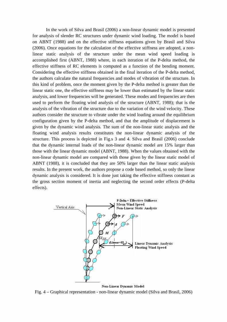
In the work of Silva and Brasil (2006) a non-linear dynamic model is presented for analysis of slender RC structures under dynamic wind loading. The model is based on ABNT (1988) and on the effective stiffness equations given by Brasil and Silva (2006). Once equations for the calculation of the effective stiffness are adopted, a non-linear static analysis of the structure under the mean wind speed loading is accomplished first (ABNT, 1988) where, in each iteration of the P-delta method, the effective stiffness of RC elements is computed as a function of the bending moment. Considering the effective stiffness obtained in the final iteration of the P-delta method, the authors calculate the natural frequencies and modes of vibration of the structure. In this kind of problem, once the moment given by the P-delta method is greater than the linear static one, the effective stiffness may be lower than estimated by the linear static analysis, and lower frequencies will be generated. These modes and frequencies are then used to perform the floating wind analysis of the structure (ABNT, 1988); that is the analysis of the vibration of the structure due to the variation of the wind velocity. These authors consider the structure to vibrate under the wind loading around the equilibrium configuration given by the P-delta method, and that the amplitude of displacement is given by the dynamic wind analysis. The sum of the non-linear static analysis and the floating wind analysis results constitutes the non-linear dynamic analysis of the structure. This process is depicted in Fig.s 3 and 4. Silva and Brasil (2006) conclude that the dynamic internal loads of the non-linear dynamic model are 15% larger than those with the linear dynamic model (ABNT, 1988). When the values obtained with the non-linear dynamic model are compared with those given by the linear static model of ABNT (1988), it is concluded that they are 50% larger than the linear static analysis results. In the present work, the authors propose a code based method, so only the linear dynamic analysis is considered. It is done just taking the effective stiffness constant as the gross section moment of inertia and neglecting the second order effects (P-delta effects).

Fig. 4 – Graphical representation - non-linear dynamic model (Silva and Brasil, 2006)

For the optimization process, the augmented Lagrangian method for dynamic

response optimization problems as described by Chahande and Arora (1994) and Arora (2004) is used. This method transforms a constrained optimization problem into an unconstrained optimization problem. The objective and constraints functions are combined using the Lagrange multipliers and penalty parameters to create an augmented Lagrangian functional. A sequence of functionals is created by properly altering the penalty parameters and Lagrange multipliers. The unconstrained minimum value of the functional in this sequence converges to the minimum of the constrained problem. Considering all the methods describe in this section we developed the work here presented. 3. LINEAR DYNAMIC ANALYSIS 3.1 Linear Static Analysis (LSA)

According to ABNT (1988), V0 (m/s) is the mean wind speed computed based on a 3 s interval, at 10 m above ground, for a plain terrain with no roughness, and a return period of 50 years. The topographic factor is S1, while the terrain roughness factor is S2, given as

p

r zbFS )10(2 = (1) where b, p and Fr are factors that depend on the terrain characteristics and z is the height above ground in meters. Factors S1, S2 and S3 are given in tables in ABNT (1988). The characteristic wind speed (m/s) and the wind pressure (Pa), respectively, are

3210 SSSVVk = and 2613.0 kVq = . (2)

The wind load (N) on an area A (projected area on a vertical plane of the given object in m2) is computed as

AqCF a= , (3)

where Ca is the drag coefficient. ABNT (1988) presents tables for Ca values. 3.2 Linear Dynamic Analysis (LDA) If the first natural frequency of vibration of a given structure is smaller than 1 Hz, it is necessary to perform dynamic analysis of the structure (ABNT, 1988). According ABNT (1988), the dynamic analysis is performed as follows. For the j-th degree of freedom, the total load Xj due to direct wind along the tower is the sum of the mean and the floating loads given as:

jjj XXX ˆ+= . (4)

The mean load jX is given as

p

r

jjjoj z

zACbqX

22

⎟⎟⎠

⎞⎜⎜⎝

⎛= , (5)

where

2613.0 po Vq = and 31069.0 SSVVp = ( oq in N/m2 and pV in m/s), (6) and b and p are given in Table 20 in ABNT (1988); zr is the reference height, taken as 10 m in this work; pV is the design wind speed corresponding to the mean speed during

10 minutes at 10 m above the ground for a terrain roughness (S2) for category II. The floating component jX̂ in Eq. (4) is given as

jjHj FX ϕψ=ˆ (7) where

o

jj m

m=ψ , ξ

ϕψ

ϕβ

∑

∑

=

==n

iii

n

iii

ooH AbqF

1

2

12 , p

r

i

o

iaii z

zAAC ⎟⎟

⎠

⎞⎜⎜⎝

⎛=β (8)

and mi, m0, Ai, A0, ξ and Cai are the lumped mass at the i-th degree of freedom, a reference mass, the equivalent area at the i-th degree of freedom, a reference area, the dynamic coefficient of amplification in Figs. 14 to 18 of ABNT (1988), and the drag coefficient for area Ai, respectively. Note that ϕ = [ϕi] is a given mode of vibration. To compute ϕi and ξ, it is necessary to consider the structural mass and stiffness. The damping factor ζ is given by ABNT (1988). When the section varies in function of the diameter ζ = 1.5 and for cylindrical structures ζ = 1.0. The lumped mass can be easily calculated by summing the mass around the influence region of a node. The total homogenized moment of inertia of the cross-section is given as

hom total sG III += , )1(sec

hom −=c

sss E

EII , ) ( 560085.0sec MPafE ckc ×= , (9)

where Es, Ec sec, Is, Is hom, IG and fck are the elasticity modulus of steel, the secant elasticity modulus of concrete (ABNT, 2003), the moment of inertia about the structural axis of the total longitudinal steel area, the homogenized moment of inertia of the longitudinal steel area, the gross moment of inertia of the cross-section, and the characteristic compressive resistance in MPa for 28 days old concrete, respectively. In the linear dynamic analysis here accomplished, we consider the cross-sectional moment of inertia as,

IEF = IG, (10)

 

of each section to compute stiffness matrix of the structure. We consider that the structure under linear static behavior does not suffer any plastification or irreversible cracking. Consider a given vector iQ̂ which represents a quantity such as internal loads,

stress, or strain, due to the i-th natural mode of vibration. The contribution Q̂ of r modes in the dynamic analysis is computed as

2/1

1

2ˆˆ⎥⎦

⎤⎢⎣

⎡= ∑

=

r

kiQQ , while ii XY

31

= (11)

is the transverse load, due to the variation of the wind direction. The first expression of Eq. (11) is called simply the RSS method, which means square root of the sum of the squares method. 4. THE AUGMENTED LAGRANGIAN METHOD

To solve the structural optimization problem formulated in this paper, it is necessary to adopt optimization algorithms that deal with static and dynamic constraints, as well as non-linear functions. A non-linear optimization problem with static and dynamic constraints is presented as follows: find the design variables b∈ nR that minimize the non-linear objective function f(b) subjected to the non-linear constraint functions:

Static l,=i ;)(ig 10=b

(12) m,+l=i ;)(g i 10≤b (13)

and dynamic, ∀ t ∈ [t0,tf],

l',+m=i ;=t)(t),(t),(t),,(gt),(g ii 10zz &&&zbb = (14) m',l'+=i ;t)(t),(t),(t),,(gt),(g ii 10≤= zz &&&zbb (15)

In dynamics of structures, the displacement vector z(t) must satisfy the equations of motion, a system of second-order ordinary differential equations:

),,,,(),,,,(+)(),,,,(+)(),,,,( tttttt zzzzzz zzbpzzbRzzbCzzbM &&&&&&&&&&&&&&& = (16)

with the initial conditions as 0000 )(and )( zz zz == tt && . Here M ),,,,( tzzzb &&& and C ),,,,( tzzzb &&& are the mass and damping matrices, respectively; the vector R ),,,,( tzzzb &&& is the generalized elastic force; and p ),,,,( tzzzb &&& is the generalized force vector. Equations (12) and (13) include, for example, limits of the design variables. Equations (14) and (15) represent constraints on dynamic response such as the maximum and minimum values of the displacements z(t), dynamic strain and stress. The initial and final times are t0 and tf , respectively.

During the design process, a set of parameters, denoted as design variables b, are selected to define the system. Once the design variables are specified, the vector z(t) is determined by Eq. (16). The displacements are called state variables, as they determine the structure configuration for every t ∈ [t0,tf], and Eq. (16) is the state equation. The constraints on dynamic response are explicit functions of state variables and implicit functions of the design variables. Usually, in structural optimization problems with dynamic constraints, the state variables vector is denoted as z(t). In this work, we use an equivalent static method where the analysis is done by computing the maximum amplitude of each mode of vibration and then using the RSS method, as shown previously in Eq. (11).

There are several optimization methods to solve the problem defined by Eqs. (12) to (16). We treat this problem using the augmented Lagrangian method where an augmented functional is created using the objective and the constraint functions:

),),(P()f(),,( rubgbrub +=Φ (17)

P(g(b),u,r) is a penalty functional, and u R∈ m' and r R∈ m' are the Lagrange multipliers and the penalty parameters, respectively. It is possible to determine u* and r* so that the minimum point b* of the functional defined in Eq. (17) is the minimum point of the problem defined by Eqs. (12) to (16). As we use iterative methods to find u* and r*, it is necessary to use a stopping criterion.

The augmented Lagrangian method defines procedures for updating penalty parameters and Lagrange multipliers. This method can be simply described by the algorithm:

Step 1. Set k=0, estimate vector u and r. Step 2. Minimize Φ(b,uk,rk) with respect to b. Let bk be the best point obtained in

this step. Step 3. If the stopping criterion is satisfied, stop the iterative process. Step 4. Update uk and rk if necessary. Step 5. Set k=k+1 and go to Step 2.

The multipliers method is quite simple, and its essence is contained in Steps 2 and 4. The functional in Eq. (17) can be defined in several ways. In the present work, the Lagrangian functional adopted to solve the problem with dynamic response is defined as:

( ) ( )

( ) ( ) dttgrtgr

grgrf

ft

t

m

liiii

l

miiii

m

liiii

l

iiii

∫ ∑∑

∑∑

⎭⎬⎫

⎩⎨⎧

+++

+⎭⎬⎫

⎩⎨⎧

++++=Φ

+=+

+=

+=+

=

0

'

1'

2'

1

2

1

2

1

2

),(),(21

)()(21 )(),(

θθ

θθ

bb

bbbrb ,θ

(18) In Eq. (18) ri represents the penalty parameters and θi defines the Lagrangian multipliers as ui = riθi, for i=1,...,m’. Note that, in Eq. (18), the dynamic constraint functions are integrated over the time interval and combined with the objective function to obtain the Lagrangian functional. At Steps 2 and 3, it is necessary to adopt a stopping criterion. Here, we consider the following stopping criterion:

K < p, (19) where p is the maximum number of iterations, and

ε≤Φ∇ ),,( krub kk

and (20)

εθ

θ

≤−

−=

≤≤≤≤+≤≤≤≤

≤≤+≤≤

} |)

|;) |;| i

(t))t),,(max(g| max( max|);t),(g| max( max

),(max(g| max)(gmax maxK

i(k)

itttm'il

(k)itttl'i

(k)imil

(k)ilib

f0f0

bb

bb

1'1

11{

(21)

[ ] ε≤ΦΦ−Φ +++ ),,(/),,(),,( 11 kk1k rubrubrub kkkkkk

(22) In Eq. (21) Kb is the maximum constraint violation, and in Eqs. (20) to (22) ε is the tolerance. If the algorithm is not converging, the condition in Eq. (19) states a finite number of iterations. Chahande and Arora (1994) noted in several examples analyzed that the best value for p is 2n. The process of updating the Lagrange multipliers and penalty parameters and more details on the adopted algorithm are presented by Arora (2004) and Chahande and Arora (1994). In the work of Chahande and Arora (1994), only Eq. (21) is suggested as the stopping criterion, but in this work, based on tests accomplished by the authors, we adopt other conditions as well.

A computer program was developed, based on the augmented Lagrangian method. The following numerical methods were utilized to implement this method:

- to solve the equations of motion (16), we use the procedure given in Section 2 for non-linear analysis;.

- related to unconstrained minimization (Step 2), we use the conjugate gradient method with Armijo line search;

- to calculate the gradient vector, we use the finite difference method; - to solve linear systems, we use Cholesky decomposition.

5. DESCRIPTION OF THE STRUCTURES

The RC towers analyzed here presents height varying from 20 m to 60 m with a circular cross-section. Based on that, we suggest that the results given here be used only to structures with height no larger than 60 m. The diameter, thickness and steel areas may change along the height of the tower and are different from one tower to the other. The concrete used in the fabrication of the tower has a characteristic resistance at 28 days (fck) as 45 MPa, which gives secant elasticity modulus (Ecsec) of 31.9 GPa from Eq. (9). Applying the safety factor, the concrete design resistance is then fcd = 45/1.3 MPa. The steel has a cover of 25 mm, design resistance of fyd = 500/1.15 MPa and elasticity modulus Es = 210 GPa.

The structures are discretized with 41 nodes and 40 elements. The first element starts at the first node and ends at the second, the second element starts at the second node and ends at the third, and so on. With this discretization, the structure has 240 degrees of freedom. The displacement vector corresponding to the structural degrees of freedom is also denoted as the state variable vector. Fig. 5 shows a typical structure cross-section, where ø, e, As and Asw are respectively the external diameter, thickness, the longitudinal steel area and the traverse reinforcement.

Fig. 5 – Cross-section

As the ninety structures analyzed here are installed in several places in Brazil,

the basic wind speed V0, topographic factor S1 and terrain roughness S2 ≡ (b; p; Fr), are adopted according to the local of installation. The statistical factor is S3 = 1.1. As stated before, the wind load on an area A is AqCF a= , where Ca represents the drag coefficients. Several pieces of equipment are installed on the structure, such as a ladder with anti-fall cable, a platform with antenna supports, night signer lights, a system of protection against lightning, and antennas. The values of A and Ca changes from tower to tower.

Besides these areas and drag coefficients, the tower mass is considered distributed along the structure proportionally to the volume and can be computed using

a density of 2500 kg/m3. The masses of the other components are also considered. As the goal of the paper is to compare the static with the dynamic internal loads, specially the bending moment, these data are not important to the final result of the work.

5. COMPUTATION OF THE DYNAMIC MAGNIFICATION FACTOR To explain the methodology and the results obtained here, let’s take as example

a 40 m tall structure, whose diameter varies along the height. In this case, the damping factor ζ = 1.5 (ABNT, 1988). Accomplishing a dynamic finite element analysis, we compute the first natural frequency of vibration f1 = 0.42 Hz. The wind factors are V0 = 40 m/s, topographic factor S1 = 1.0, and terrain roughness S2 ≡ III and the statistical factor is S3 = 1.1. The structure is loaded with antennas, supports, platforms, cables, ladder, etc. After analyzing this structure considering the static and dynamic models we obtain the bending moments given in Table 1. Note that the results of some nodes were suppressed to reduce the size of the table.

Table 1 – Internal loads of a given 40 m tall structure Node (i) z (m) Mlsad (kN.m) Mldad (kN.m) γd

1 40,0 0,00 0,002 39,0 19,40 16,20 0,833 38,0 39,82 35,18 0,884 37,0 61,27 56,84 0,93

10 31,0 212,00 241,07 1,1420 21,0 550,32 730,47 1,3326 15,0 807,20 1109,14 1,3727 14,0 853,96 1176,92 1,3828 13,0 901,85 1245,82 1,3829 12,0 950,87 1315,77 1,3830 11,0 1000,99 1386,70 1,3931 10,0 1052,22 1458,51 1,3932 9,0 1104,54 1531,13 1,3933 8,0 1157,91 1604,48 1,3934 7,0 1212,33 1678,49 1,3835 6,0 1267,76 1753,09 1,3836 5,0 1324,18 1828,20 1,3837 4,0 1381,56 1903,78 1,3838 3,0 1439,85 1979,75 1,3739 2,0 1499,02 2056,01 1,3740 1,0 1558,76 2132,47 1,3741 0,0 1619,01 2209,14 1,36

resume 100% 138% 1,38

In this Table, z is the height above ground, while Mlsad and Mldad are the design bending moments given, respectively, by the linear static analysis and linear dynamic analysis. We consider the bending moment to develop the methodology proposed here because it is the most important internal load in this kind of structure. The magnification factor γd(i) of a given section (i) is computed as

)()(

)(iMiM

ilsad

ldadd =γ (23)

Fig. 6 – Dynamic and static flexure moment along the structure axis

The magnification factor of the structure γd is the average of γd(i) computed in the results of nodes 27 to 41 (approximately the one third of structure near to the ground level):

∑=

=41

27)(

151

idd iγγ (24)

In Table 1, in the resume line, 100% means the result of the static analysis while 138% is the ratio between the dynamic and static results. It means that the dynamic flexure moment is 38% larger than the static flexure moment (average in the third part of the structure near to the ground level). So γd, defined here as the dynamic magnification factor, is the factor that can be used to find directly the dynamic results of a given tower. In Fig. 6 are shown these flexure moments along the structure axis. Table 2 – Values of γd for ζ = 1.5 and S2 = III

H (m) f1 (Hz) γd γd0 γd1 γd2 E0 E1 E220 0,97 1,28 1,44 1,28 1,30 0,012 0,000 0,00030 0,45 1,38 1,44 1,40 1,38 0,002 0,000 0,00040 0,31 1,42 1,44 1,46 1,45 0,000 0,001 0,00150 0,20 1,56 1,44 1,51 1,54 0,007 0,001 0,00060 0,19 1,53 1,44 1,55 1,53 0,004 0,000 0,00020 1,15 1,27 1,44 1,25 1,27 0,014 0,000 0,00030 0,54 1,36 1,44 1,38 1,35 0,003 0,000 0,00040 0,42 1,38 1,44 1,44 1,38 0,002 0,002 0,00050 0,28 1,50 1,44 1,50 1,47 0,002 0,000 0,00060 0,23 1,49 1,44 1,54 1,50 0,002 0,001 0,00020 0,65 1,34 1,44 1,33 1,33 0,004 0,000 0,00030 0,39 1,42 1,44 1,41 1,40 0,000 0,000 0,00040 0,26 1,45 1,44 1,46 1,48 0,000 0,000 0,00150 0,17 1,59 1,44 1,51 1,57 0,012 0,003 0,00060 0,14 1,58 1,44 1,55 1,59 0,011 0,000 0,000

total error 0,086 0,075 0,009 0,002

Adopting the same procedure for several structures and grouping those that present the same value of ζ and S2, we can build a table similar to Table 2. In this table H is the structure height, f1 is the first natural frequency of vibration and γd the dynamic magnification factor. Consider now that γd is written approximately as:

⎪⎩

⎪⎨

⎧

+++++=→=++=→=

=→=≅

21

2112

11

0

21

0 where,

ffeHdHfcfbHakcfbHak

ak

d

d

d

dkd

γγ

γγγ (25)

In Eq. (25) we note that for k = 0 the approximation of γd is given by a constant function, when k = 1 by a linear function and for k = 2 by a quadratic equation. Considering the approximations given by Eq. (25), we define the following design variables of the optimization problem to determinate the dynamic magnification factor:

[ ]

[ ][ ]⎪⎩

⎪⎨

⎧=

fedcbacba

ab . (26)

Consider respectively the real and approximated dynamic magnification factor vectors γd and γdk of a given group of structures which present the same ζ and S2. The quadratic error between the approximation γdk and the real factor γd is:

∑=

−=j

ididkikE

1

2))( (21)( γγ bb . (27)

Once that γdki, is computed according to one of Eq. (25), always generates an approximation error in (27), the problem of minimizing this error is an optimization problem. We formulate the following optimization problems: determine b that Minimize Ek(b) Subjected to jidki ,...,1 0)( =≥bγ (28) Note that for k = 0 we have one optimization problem, k = 1 other problem and so on, and that the value of j is 15. The optimization problems presented here are of inverse analysis. As we mentioned in the present work, we analyzed a total of ninety towers and computed the real dynamic magnification factor vectors of groups of these towers with same ζ and S2. These vectors were used to compute the approximation dynamic magnification factor.

Coming back to Table 2, γd0 is the approximation of the constant function, while γd1 and γd2 are the approximations given by the linear and quadratic functions respectively. The same way, E0, E1 and E2 are respectively the approximation errors of constant, linear and quadratic functions. One can note that column E2 is the one that presents the smallest errors. However, in some cases, when the height is larger than 60 m the value of γd2 can present non-realistic values. Because of that, we suggest to the readers and engineers that use the method to adopt the linear approximation γd1 and only consider the results presented here in structures no longer than 60 m. In Tables 3 to 8 are shown the coefficients of γdk for several values of ζ and S2.

Table 3 – Coefficients of γdk for ζ = 1.5 and S2 = II

Design Variablesfunction a b c d e f

0 1,5963971 1,592341 0,002299 ‐0,208512 1,095788 0,026414 0,632866 ‐0,03026 ‐0,00021 ‐0,11634

Fig. 7 – Dynamic magnification factor γd1 for ζ = 1.5 and S2 = II

Table 4 – Coefficients of γdk for ζ = 1.5 and S2 = III

Design Variablesk a b c d e f0 1,4363331 1,3615 0,003594 ‐0,163392 0,943021 0,02439 0,575259 ‐0,02768 ‐0,00018 ‐0,08937

Fig. 8 – Dynamic magnification factor γd1 for ζ = 1.5 and S2 = III

Table 5 – Coefficients of γdk for ζ = 1.5 and S2 = IV

Design Variablesfunction a b c d e f

0 1,2630541 1,172087 0,003751 ‐0,140042 0,79765 0,022412 0,50859 ‐0,02418 ‐0,00017 ‐0,08094  

Fig. 9 – Dynamic magnification factor γd1 for ζ = 1.5 and S2 = IV

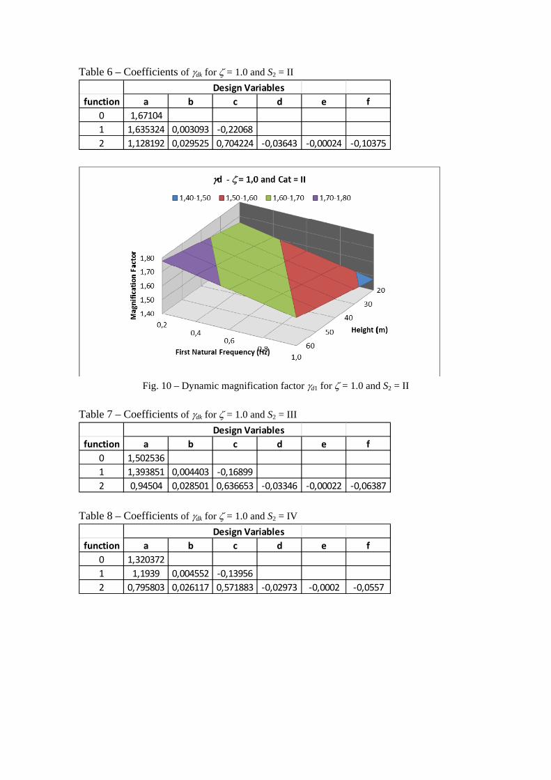
Table 6 – Coefficients of γdk for ζ = 1.0 and S2 = II Design Variables

function a b c d e f0 1,671041 1,635324 0,003093 ‐0,220682 1,128192 0,029525 0,704224 ‐0,03643 ‐0,00024 ‐0,10375  

 

 Fig. 10 – Dynamic magnification factor γd1 for ζ = 1.0 and S2 = II

 Table 7 – Coefficients of γdk for ζ = 1.0 and S2 = III

Design Variablesfunction a b c d e f

0 1,5025361 1,393851 0,004403 ‐0,168992 0,94504 0,028501 0,636653 ‐0,03346 ‐0,00022 ‐0,06387

Table 8 – Coefficients of γdk for ζ = 1.0 and S2 = IV

Design Variablesfunction a b c d e f

0 1,3203721 1,1939 0,004552 ‐0,139562 0,795803 0,026117 0,571883 ‐0,02973 ‐0,0002 ‐0,0557

Fig. 11 – Dynamic magnification factor γd1 for ζ = 1.0 and S2 = III

Fig. 12 – Dynamic magnification factor γd1 for ζ = 1.0 and S2 = IV

One can note that in the results showed in the present work γd varies from 1.2 to

1.7. As we stated before, in this kind of structures, the main internal loads are the bending moment, the shear load and the axial load. Only the bending moment and the shear load are multiplied by the magnification factor to obtain the dynamic results. In cases analyzed here, the axial load is not influenced by the dynamic response. 

6. CONCLUSIONS We presented the linear static and dynamic models based on the NBR-6123 (ABNT, 1988) code to compute the wind loads. A special emphasis was placed in pre-cast RC towers. A new procedure, based on graphs and curves obtained using optimization techniques, uses the results of the static analysis to compute the dynamic response of this kind of structures. One peculiar characteristic of these pre-cast RC structures is that they often present the first natural frequency of vibration smaller than 1 Hz and so the dynamic analysis is needed. The main feature researched is the dynamic magnification factor, defined here as the ratio between the bending moment given by the dynamic and static models (ABNT, 1988). Surfaces are created to give the dynamic magnification factor as a function of the structure height and the first natural frequency of vibration. To create these surfaces, optimization problems (inverse problems) were formulated where the objective function is the error between the dynamic magnification factor, computed according to (ABNT, 1988), and other given by equations, defined in function of the structure height and first natural frequency of vibration. The design variables are the coefficients of these equations and constraints are imposed to avoid negative and also very large frequencies. With the methodology proposed here only the static results and the first natural frequency of vibration are need to accomplish the dynamic analysis of a given structure. The method is easier and faster than the tradition dynamic analysis approach. In this work, results of the dynamic and static analysis of 90 real structures are used in the optimization process. The methodology proposed here is quite precise and can reduce drastically engineering and computational time used to accomplish the dynamic analysis of RC Telecommunication Towers. Thus, the graphs created by the authors constitute a new tool that can easily be used by Engineers. As suggestions for futures works we state the determination of a simplified model that takes into consideration the non-linearities of the structure  

REFERENCES ABNT – Associação Brasileira de Normas Técnicas, (1988), NBR-6123 - Forças

Devidas ao Vento em Edificações (in portuguese). ABNT – Associação Brasileira de Normas Técnicas, (2003), NBR-6118 - Projeto de

Obras de Concreto (in portuguese). ACI – American Concrete Institute, (1971), ACI Committee 318 - Building Code

Requirements for Reinforced Concrete, Detroit. Arora, J. S., (2004), Introduction to Optimum Design, Second Edition, Elsevier

Academic Press. Branson, D. E., (1963). Instantaneous and Time-Dependent Deflections of Simple and

Continuous Reinforced Concrete Beams, Report Nº. 7, Alabama Highway Research Report, Bureau of Public Roads, Aug. 1963, pp. 1-78.

Brasil, R. M. L. R. F. and Silva, M. A., (2006). RC Large Displacements: Optimization Applied To Experimental Results, Computer and Structures 84 (2006), Elsevier, pp. 1164-1171.

Chahande, A. I. and Arora, J. S., (1994). Optimization of large structures subjected to dynamic loads with the multiplier method, International Journal For Numerical Methods in Engineering, 37, pp. 413-430.

Silva, M. A. and Brasil, R. M. L. R. F., (2006). Nonlinear Dynamic Analysis Based on Experimental Data of RC Telecommunication Towers Subjected to Wind

Loading, Mathematical Problems in Engineering 2006 (2006), Article ID 46815, 10 pages.

ACKNOWLEDGEMENTS

This work is result of a research project completed during an academic visit accomplished by Marcelo Araujo da Silva at The University of Iowa, under the supervision of Prof. Jasbir S. Arora, in Iowa City, IA, USA. The program was sponsored by RM Soluções Engenharia Ltda. A great portion of the work was developed using resources of the Optimal Design Laboratory at The University of Iowa. All these supports are gratefully acknowledged.