dynamic asset allocation - auecon.au.dk/.../dynamic_asset_allocation/daacurrent.pdf · dynamic...
TRANSCRIPT

Dynamic Asset Allocation
Claus Munk
Until August 2012:
Aarhus University, e-mail: [email protected]
From August 2012:
Copenhagen Business School, e-mail: [email protected]
this version: July 3, 2012
The document contains graphs in color, use color printer for best results.


Contents
Preface v
1 Introduction to asset allocation 1
1.1 Introduction . . . . . . . . . . . . . . . . . . . . . . . . . . . . . . . . . . . . . . . . 1
1.2 Investor classes and motives for investments . . . . . . . . . . . . . . . . . . . . . . 1
1.3 Typical investment advice . . . . . . . . . . . . . . . . . . . . . . . . . . . . . . . . 3
1.4 How do individuals allocate their wealth? . . . . . . . . . . . . . . . . . . . . . . . 3
1.5 An overview of the theory of optimal investments . . . . . . . . . . . . . . . . . . . 3
1.6 The future of investment management and services . . . . . . . . . . . . . . . . . . 3
1.7 Outline of the rest . . . . . . . . . . . . . . . . . . . . . . . . . . . . . . . . . . . . 3
1.8 Notation . . . . . . . . . . . . . . . . . . . . . . . . . . . . . . . . . . . . . . . . . . 3
2 Preferences 5
2.1 Introduction . . . . . . . . . . . . . . . . . . . . . . . . . . . . . . . . . . . . . . . . 5
2.2 Consumption plans and preference relations . . . . . . . . . . . . . . . . . . . . . . 6
2.3 Utility indices . . . . . . . . . . . . . . . . . . . . . . . . . . . . . . . . . . . . . . . 9
2.4 Expected utility representation of preferences . . . . . . . . . . . . . . . . . . . . . 10
2.5 Risk aversion . . . . . . . . . . . . . . . . . . . . . . . . . . . . . . . . . . . . . . . 16
2.6 Utility functions in models and in reality . . . . . . . . . . . . . . . . . . . . . . . . 20
2.7 Preferences for multi-date consumption plans . . . . . . . . . . . . . . . . . . . . . 26
2.8 Exercises . . . . . . . . . . . . . . . . . . . . . . . . . . . . . . . . . . . . . . . . . 33
3 One-period models 37
3.1 Introduction . . . . . . . . . . . . . . . . . . . . . . . . . . . . . . . . . . . . . . . . 37
3.2 The general one-period model . . . . . . . . . . . . . . . . . . . . . . . . . . . . . . 37
3.3 Mean-variance analysis . . . . . . . . . . . . . . . . . . . . . . . . . . . . . . . . . . 43
3.4 A numerical example . . . . . . . . . . . . . . . . . . . . . . . . . . . . . . . . . . . 49
3.5 Mean-variance analysis with constraints . . . . . . . . . . . . . . . . . . . . . . . . 49
3.6 Estimation . . . . . . . . . . . . . . . . . . . . . . . . . . . . . . . . . . . . . . . . 49
i

ii Contents
3.7 Critique of the one-period framework . . . . . . . . . . . . . . . . . . . . . . . . . . 49
3.8 Exercises . . . . . . . . . . . . . . . . . . . . . . . . . . . . . . . . . . . . . . . . . 50
4 Discrete-time multi-period models 51
4.1 Introduction . . . . . . . . . . . . . . . . . . . . . . . . . . . . . . . . . . . . . . . . 51
4.2 A multi-period, discrete-time framework for asset allocation . . . . . . . . . . . . . 51
4.3 Dynamic programming in discrete-time models . . . . . . . . . . . . . . . . . . . . 54
5 Introduction to continuous-time modelling 59
5.1 Introduction . . . . . . . . . . . . . . . . . . . . . . . . . . . . . . . . . . . . . . . . 59
5.2 The basic continuous-time setting . . . . . . . . . . . . . . . . . . . . . . . . . . . . 59
5.3 Dynamic programming in continuous-time models . . . . . . . . . . . . . . . . . . 62
5.4 Loss from suboptimal strategies . . . . . . . . . . . . . . . . . . . . . . . . . . . . . 66
5.5 Exercises . . . . . . . . . . . . . . . . . . . . . . . . . . . . . . . . . . . . . . . . . 67
6 Asset allocation with constant investment opportunities 69
6.1 Introduction . . . . . . . . . . . . . . . . . . . . . . . . . . . . . . . . . . . . . . . . 69
6.2 General utility function . . . . . . . . . . . . . . . . . . . . . . . . . . . . . . . . . 70
6.3 CRRA utility function . . . . . . . . . . . . . . . . . . . . . . . . . . . . . . . . . . 72
6.4 Logarithmic utility . . . . . . . . . . . . . . . . . . . . . . . . . . . . . . . . . . . . 75
6.5 Discussion of the optimal investment strategy for CRRA utility . . . . . . . . . . . 76
6.6 The life-cycle . . . . . . . . . . . . . . . . . . . . . . . . . . . . . . . . . . . . . . . 78
6.7 Loss due to suboptimal investments . . . . . . . . . . . . . . . . . . . . . . . . . . 80
6.8 Infrequent rebalancing of the portfolio . . . . . . . . . . . . . . . . . . . . . . . . . 81
6.9 Exercises . . . . . . . . . . . . . . . . . . . . . . . . . . . . . . . . . . . . . . . . . 84
7 Stochastic investment opportunities: the general case 85
7.1 Introduction . . . . . . . . . . . . . . . . . . . . . . . . . . . . . . . . . . . . . . . . 85
7.2 General utility functions . . . . . . . . . . . . . . . . . . . . . . . . . . . . . . . . . 86
7.3 CRRA utility . . . . . . . . . . . . . . . . . . . . . . . . . . . . . . . . . . . . . . . 93
7.4 Logarithmic utility . . . . . . . . . . . . . . . . . . . . . . . . . . . . . . . . . . . . 105
7.5 How costly are deviations from the optimal investment strategy? . . . . . . . . . . 105
7.6 Exercises . . . . . . . . . . . . . . . . . . . . . . . . . . . . . . . . . . . . . . . . . 107
8 The martingale approach 111
8.1 The martingale approach in complete markets . . . . . . . . . . . . . . . . . . . . . 111
8.2 Complete markets and constant investment opportunities . . . . . . . . . . . . . . 115
8.3 Complete markets and stochastic investment opportunities . . . . . . . . . . . . . . 119
8.4 The martingale approach with portfolio constraints . . . . . . . . . . . . . . . . . . 120
8.5 Exercises . . . . . . . . . . . . . . . . . . . . . . . . . . . . . . . . . . . . . . . . . 127
9 Numerical methods for solving dynamic asset allocation problems 129

Contents iii
10 Asset allocation with stochastic interest rates 131
10.1 Introduction . . . . . . . . . . . . . . . . . . . . . . . . . . . . . . . . . . . . . . . . 131
10.2 One-factor Vasicek interest rate dynamics . . . . . . . . . . . . . . . . . . . . . . . 132
10.3 One-factor CIR dynamics . . . . . . . . . . . . . . . . . . . . . . . . . . . . . . . . 135
10.4 A numerical example . . . . . . . . . . . . . . . . . . . . . . . . . . . . . . . . . . . 137
10.5 Two-factor Vasicek model . . . . . . . . . . . . . . . . . . . . . . . . . . . . . . . . 143
10.6 Other studies with stochastic interest rates . . . . . . . . . . . . . . . . . . . . . . 146
10.7 Exercises . . . . . . . . . . . . . . . . . . . . . . . . . . . . . . . . . . . . . . . . . 149
11 Asset allocation with stochastic market prices of risk 153
11.1 Introduction . . . . . . . . . . . . . . . . . . . . . . . . . . . . . . . . . . . . . . . . 153
11.2 Mean reversion in stock returns . . . . . . . . . . . . . . . . . . . . . . . . . . . . . 153
11.3 Stochastic volatility . . . . . . . . . . . . . . . . . . . . . . . . . . . . . . . . . . . 160
11.4 More . . . . . . . . . . . . . . . . . . . . . . . . . . . . . . . . . . . . . . . . . . . . 164
11.5 Exercises . . . . . . . . . . . . . . . . . . . . . . . . . . . . . . . . . . . . . . . . . 164
12 Inflation risk and asset allocation with no risk-free asset 167
12.1 Introduction . . . . . . . . . . . . . . . . . . . . . . . . . . . . . . . . . . . . . . . . 167
12.2 Real and nominal price dynamics . . . . . . . . . . . . . . . . . . . . . . . . . . . . 167
12.3 Constant investment opportunities . . . . . . . . . . . . . . . . . . . . . . . . . . . 169
12.4 General stochastic investment opportunities . . . . . . . . . . . . . . . . . . . . . . 172
12.5 Hedging real interest rate risk without real bonds . . . . . . . . . . . . . . . . . . . 172
13 Labor income 179
13.1 Introduction . . . . . . . . . . . . . . . . . . . . . . . . . . . . . . . . . . . . . . . . 179
13.2 A motivating example . . . . . . . . . . . . . . . . . . . . . . . . . . . . . . . . . . 179
13.3 Exogenous income in a complete market . . . . . . . . . . . . . . . . . . . . . . . . 181
13.4 Exogenous income in incomplete markets . . . . . . . . . . . . . . . . . . . . . . . 189
13.5 Endogenous labor supply and income . . . . . . . . . . . . . . . . . . . . . . . . . . 191
13.6 More . . . . . . . . . . . . . . . . . . . . . . . . . . . . . . . . . . . . . . . . . . . . 194
14 Consumption and portfolio choice with housing 195
15 Other variations of the problem... 197
15.1 Multiple and/or durable consumption goods . . . . . . . . . . . . . . . . . . . . . . 197
15.2 Uncertain time of death; insurance . . . . . . . . . . . . . . . . . . . . . . . . . . . 197
16 International asset allocation 199
17 Non-standard assumptions on investors 201
17.1 Preferences with habit formation . . . . . . . . . . . . . . . . . . . . . . . . . . . . 201
17.2 Recursive utility . . . . . . . . . . . . . . . . . . . . . . . . . . . . . . . . . . . . . 203
17.3 Model/parameter uncertainty, incomplete information, learning . . . . . . . . . . . 210
17.4 Ambiguity aversion . . . . . . . . . . . . . . . . . . . . . . . . . . . . . . . . . . . . 210
17.5 Other objective functions . . . . . . . . . . . . . . . . . . . . . . . . . . . . . . . . 210
17.6 Consumption and portfolio choice for non-price takers . . . . . . . . . . . . . . . . 210

iv Contents
17.7 Non-utility based portfolio choice . . . . . . . . . . . . . . . . . . . . . . . . . . . . 210
17.8 Allowing for bankruptcy . . . . . . . . . . . . . . . . . . . . . . . . . . . . . . . . . 211
18 Trading and information imperfections 213
18.1 Trading constraints . . . . . . . . . . . . . . . . . . . . . . . . . . . . . . . . . . . . 213
18.2 Transaction costs . . . . . . . . . . . . . . . . . . . . . . . . . . . . . . . . . . . . . 213
A Results on the lognormal distribution 219
B Stochastic processes and stochastic calculus 223
B.1 Introduction . . . . . . . . . . . . . . . . . . . . . . . . . . . . . . . . . . . . . . . . 223
B.2 What is a stochastic process? . . . . . . . . . . . . . . . . . . . . . . . . . . . . . . 224
B.3 Brownian motions . . . . . . . . . . . . . . . . . . . . . . . . . . . . . . . . . . . . 231
B.4 Diffusion processes . . . . . . . . . . . . . . . . . . . . . . . . . . . . . . . . . . . . 234
B.5 Ito processes . . . . . . . . . . . . . . . . . . . . . . . . . . . . . . . . . . . . . . . 237
B.6 Stochastic integrals . . . . . . . . . . . . . . . . . . . . . . . . . . . . . . . . . . . . 237
B.7 Ito’s Lemma . . . . . . . . . . . . . . . . . . . . . . . . . . . . . . . . . . . . . . . . 241
B.8 Important diffusion processes . . . . . . . . . . . . . . . . . . . . . . . . . . . . . . 242
B.9 Multi-dimensional processes . . . . . . . . . . . . . . . . . . . . . . . . . . . . . . . 249
B.10 Change of probability measure . . . . . . . . . . . . . . . . . . . . . . . . . . . . . 255
B.11 Exercises . . . . . . . . . . . . . . . . . . . . . . . . . . . . . . . . . . . . . . . . . 258
C Solutions to Ordinary Differential Equations 261
References 263

Preface
INCOMPLETE!
Preliminary and incomplete lecture notes intended for use at an advanced master’s level or
an introductory Ph.D. level. I appreciate comments and corrections from Kenneth Brandborg,
Jens Henrik Eggert Christensen, Heine Jepsen, Thomas Larsen, Jakob Nielsen, Nicolai Nielsen,
Kenneth Winther Pedersen, Carsten Sørensen, and in particular Linda Sandris Larsen. Additional
comments and suggestions are very welcome!
Claus Munk
Internet homepage: sites.google.com/site/munkfinance
v


CHAPTER 1
Introduction to asset allocation
1.1 Introduction
Financial markets offer opportunities to move money between different points in time and dif-
ferent states of the world. Investors must decide how much to invest in the financial markets and
how to allocate that amount between the many, many available financial securities. Investors can
change their investments as time passes and they will typically want to do so for example when
they obtain new information about the prospective returns on the financial securities. Hence, they
must figure out how to manage their portfolio over time. In other words, they must determine an
investment strategy or an asset allocation strategy. The term asset allocation is sometimes used for
the allocation of investments to major asset classes, e.g., stocks, bonds, and cash. In later chapters
we will often focus on this decision, but we will use the term asset allocation interchangeably with
the terms optimal investment or portfolio management.
It is intuitively clear that in order to determine the optimal investment strategy for an investor,
we must make some assumptions about the objectives of the investor and about the possible returns
on the financial markets. Different investors will have different motives for investments and hence
different objectives. In Section 1.2 we will discuss the motives and objectives of different types
of investors. We will focus on the asset allocation decisions of individual investors or households.
Individuals invest in the financial markets to finance future consumption of which they obtain
some felicity or utility. We discuss how to model the preferences of individuals in Chapter 2.
1.2 Investor classes and motives for investments
We can split the investors into individual investors (households; sometimes called retail investors)
and institutional investors (includes both financial intermediaries – such as pension funds, insurance
companies, mutual funds, and commercial banks – and manufacturing companies producing goods
or services). Different investors have different objectives. Manufacturing companies probably invest
mostly in short-term bonds and deposits in order to manage their liquidity needs and avoid the
1

2 Chapter 1. Introduction to asset allocation
deadweight costs of raising small amounts of capital very frequently. They will rarely set up long-
term strategies for investments in the financial markets and their financial investments constitute
a very small part of the total investments.
Individuals can use their money either for consumption or savings. Here we use the term savings
synonymously with financial investments so that it includes both deposits in banks and investments
in stocks, bonds, and possibly other securities. Traditionally most individuals have saved in form
of bank deposits and maybe government bonds, but in recent years there has been an increasing
interest of individuals for investing in the stock market. Individuals typically save when they
are young by consuming less than the labor income they earn, primarily in order to accumulate
wealth they can use for consumption when they retire. Other motives for saving is to be able to
finance large future expenditures (e.g., purchase of real estate, support of children during their
education, expensive celebrations or vacations) or simply to build up a buffer for “hard times”
due to unemployment, disability, etc. We assume that the objective of an individual investor is
to maximize the utility of consumption throughout the life-time of the investor. We will discuss
utility functions in Chapter 2.
A large part of the savings of individuals are indirect through pension funds and mutual funds.
These funds are the major investors in today’s markets. Some of these funds are non-profit funds
that are owned by the investors in the fund. The objective of such funds should represent the
objectives of the fund investors.
Let us look at pension funds. One could imagine a pension fund that determines the optimal
portfolio of each of the fund investors and aggregates over all investors to find the portfolio of the
fund. Each fund investor is then allocated the returns on his optimal portfolio, probably net of
some servicing fee. The purpose of forming the fund is then simply to save transaction costs. A
practical implementation of this is to let each investor allocate his funds among some pre-selected
portfolios, for example a portfolio mimicking the overall stock market index, various portfolios of
stocks in different industries, one or more portfolios of government bonds (e.g., one in short-term
and one in long-term bonds), portfolios of corporate bonds and mortgage-backed bonds, portfolios
of foreign stocks and bonds, and maybe also portfolios of derivative securities and even non-financial
portfolios of metals and real estate. Some pension funds operate in this way and there seems to be
a tendency for more and more pension funds to allow investor discretion with regards to the way
the deposits are invested.
However, in many pension funds some hired fund managers decide on the investment strategy.
Often all the deposits of different fund members are pooled together and then invested according
to a portfolio chosen by the fund managers (probably following some general guidelines set up by
the board of the fund). Once in a while the rate of return of the portfolio is determined and the
deposit of each investor is increased according to this rate of return less some servicing fee. In
many cases the returns on the portfolio of the fund are distributed to the fund members using more
complicated schemes. Rate of return guarantees, bonus accounts,.... The salary of the manager of
a fund is often linked to the return on the portfolio he chooses and some benchmark portfolio(s).
A rational manager will choose a portfolio that maximizes his utility and that portfolio choice may
be far from the optimal portfolio of the fund members....
Mutual funds...
This lecture note will focus on the decision problem of an individual investor and aims to analyze

1.3 Typical investment advice 3
and answer the following questions:
• What are the utility maximizing dynamic consumption and investment strategies of an indi-
vidual?
• What is the relation between optimal consumption and optimal investment?
• How are financial investments optimally allocated to different asset classes, e.g., stocks and
bonds?
• How are financial investments optimally allocated to single securities within each asset class?
• How does the optimal consumption and investment strategies depend on, e.g., risk aversion,
time horizon, initial wealth, labor income, and asset price dynamics?
• Are the recommendations of investment advisors consistent with the theory of optimal in-
vestments?
1.3 Typical investment advice
TO COME... References: Quinn (1997), Siegel (2002)
Concerning the value of analyst recommendations: Barber, Lehavy, McNichols, and Trueman
(2001), Jegadeesh and Kim (2006), Malmendier and Shanthikumar (2007), Elton and Gruber
(2000)
1.4 How do individuals allocate their wealth?
TO COME...
References: Friend and Blume (1975), Bodie and Crane (1997), Heaton and Lucas (2000),
Vissing-Jørgensen (2002), Ameriks and Zeldes (2004), Gomes and Michaelides (2005), Campbell
(2006), Calvet, Campbell, and Sodini (2007), Curcuru, Heaton, Lucas, and Moore (2009), Wachter
and Yogo (2010)
Christiansen, Joensen, and Rangvid (2008): differences due to education
Yang (2009): house owners vs. non-owners
1.5 An overview of the theory of optimal investments
TO COME...
1.6 The future of investment management and services
TO COME... References: Bodie (2003), Merton (2003)
1.7 Outline of the rest
1.8 Notation
Since we are going to deal simultaneously with many financial assets, it will often be mathe-
matically convenient to use vectors and matrices. All vectors are considered column vectors. The

4 Chapter 1. Introduction to asset allocation
superscript > on a vector or a matrix indicates that the vector or matrix is transposed. We will
use the notation 1 for a vector where all elements are equal to 1; the dimension of the vector will
be clear from the context. We will use the notation ei for a vector (0, . . . , 0, 1, 0, . . . , 0)> where
the 1 is entry number i. Note that for two vectors x = (x1, . . . , xd)> and y = (y1, . . . , yd)
> we
have x>y = y>x =∑di=1 xiyi. In particular, x>1 =
∑di=1 xi and e>
i x = xi. We also define
‖x‖2 = x>x =∑di=1 x
2i .
If x = (x1, . . . , xn) and f is a real-valued function of x, then the (first-order) derivative of f
with respect to x is the vector
f ′(x) ≡ fx(x) =
(∂f
∂x1
, . . . ,∂f
∂xn
)>
.
This is also called the gradient of f . The second-order derivative of f is the n× n Hessian matrix
f ′′(x) ≡ fxx(x) =
∂2f∂x2
1
∂2f∂x1∂x2
. . . ∂2f∂x1∂xn
∂2f∂x2∂x1
∂2f∂x2
2. . . ∂2f
∂x2∂xn...
.... . .
...∂2f
∂xn∂x1
∂2f∂xn∂x2
. . . ∂2f∂x2n
.
If x and a are n-dimensional vectors, then
∂
∂x(a>x) =
∂
∂x(x>a) = a.
If x is an n-dimensional vector and A is a symmetric [i.e., A = A>] n× n matrix, then
∂
∂x
(x>Ax
)= 2Ax.
If A is non-singular, then (AA>)−1 = (A>)−1A−1.

CHAPTER 2
Preferences
2.1 Introduction
In order to say anything concrete about the optimal investments of individuals we have to
formalize the decision problem faced by individuals. We assume that individuals have preferences
for consumption and must choose between different consumption plans, i.e., plans for how much to
consume at different points in time and in different states of the world. The financial market allows
individuals to reallocate consumption over time and over states and hence obtain a consumption
plan different from their endowment.
Although an individual will typically obtain utility from consumption at many different dates
(or in many different periods), we will first address the simpler case with consumption at only
one future point in time. In such a setting a “consumption plan” is simply a random variable
representing the consumption at that date. Even in one-period models individuals should be
allowed to consume both at the beginning of the period and at the end of the period, but we will
first ignore the influence of current consumption on the well-being of the individual. We do that
both since current consumption is certain and we want to focus on how preferences for uncertain
consumption can be represented, but also to simplify the notation and analysis somewhat. Since
we have in mind a one-period economy, we basically have to model preferences for end-of-period
consumption.
Sections 2.2–2.4 discuss how to represent individual preferences in a tractable way. We will
demonstrate that under some fundamental assumptions (“axioms”) on individual behavior, the
preferences can be modeled by a utility index which to each consumption plan assigns a real
number with higher numbers to the more preferred plans. Under an additional axiom we can
represent the preferences in terms of expected utility, which is even simpler to work with and used
in most models of financial economics. Section 2.5 defines and discusses the important concept
of risk aversion. Section 2.6 introduces the utility functions that are typically applied in models
of financial economics and provides a short discussion of which utility functions and levels of risk
aversions that seem to be reasonable for representing the decisions of individuals. In Section 2.7
5

6 Chapter 2. Preferences
we discuss extensions to preferences for consumption at more than one point in time.
There is a large literature on how to model the preferences of individuals for uncertain outcomes
and the presentation here is by no means exhaustive. The literature dates back at least to the Swiss
mathematician Daniel Bernoulli in 1738 (see English translation in Bernoulli (1954)), but was put
on a firm formal setting by von Neumann and Morgenstern (1944). For some recent textbook
presentations on a similar level as the one given here, see Huang and Litzenberger (1988, Ch. 1),
Kreps (1990, Ch. 3), Gollier (2001, Chs. 1-3), and Danthine and Donaldson (2002, Ch. 2).
2.2 Consumption plans and preference relations
It seems fair to assume that whenever the individual compares two different consumption plans,
she will be able either to say that she prefers one of them to the other or to say that she is indifferent
between the two consumption plans. Moreover, she should make such pairwise comparisons in a
consistent way. For example, if she prefers plan 1 to plan 2 and plan 2 to plan 3, she should
prefer plan 1 to plan 3. If these properties hold, we can formally represent the preferences of the
individual by a so-called preference relation. A preference relation itself is not very tractable so
we are looking for simpler ways of representing preferences. First, we will find conditions under
which it makes sense to represent preferences by a so-called utility index which attaches a real
number to each consumption plan. If and only if plan 1 has a higher utility index than plan 2, the
individual prefers plan 1 to plan 2. Attaching numbers to each possible consumption plan is also not
easy so we look for an even simpler representation. We show that under an additional condition
we can represent preferences in an even simpler way in terms of the expected value of a utility
function. A utility function is a function defined on the set of possible levels of consumption. Since
consumption is random it then makes sense to talk about the expected utility of a consumption
plan. The individual will prefer consumption plan 1 to plan 2 if and only if the expected utility
from consumption plan 1 is higher than the expected utility from consumption plan 2. This
representation of preferences turns out to be very tractable and is applied in the vast majority of
asset pricing models.
Our main analysis is formulated under some simplifying assumptions that are not necessarily
appropriate. At the end of this section we will briefly discuss how to generalize the analysis and
also discuss the appropriateness of the axioms on individual behavior that need to be imposed in
order to obtain the expected utility representation.
We assume that there is uncertainty about how the variables affecting the well-being of an
individual (e.g., asset returns) turn out. We model the uncertainty by a probability space (Ω,F,P).
In most of the chapter we will assume that the state space is finite, Ω = 1, 2, . . . , S, so that there
are S possible states of which exactly one will be realized. For simplicity, think of this as a model
of one-period economy with S possible states at the end of the period. The set F of events that
can be assigned a probability is the collection of all subsets of Ω. The probability measure P is
defined by the individual state probabilities pω = P(ω), ω = 1, 2, . . . , S. We assume that all pω > 0
and, of course, we have that p1 + . . . pS = 1. We take the state probabilities as exogenously given
and known to the individuals.
Individuals care about their consumption. It seems reasonable to assume that when an individual
chooses between two different actions (e.g., portfolio choices), she only cares about the consumption

2.2 Consumption plans and preference relations 7
state ω 1 2 3
state prob. pω 0.2 0.3 0.5
cons. plan 1, c(1) 3 2 4
cons. plan 2, c(2) 3 1 5
cons. plan 3, c(3) 4 4 1
cons. plan 4, c(4) 1 1 4
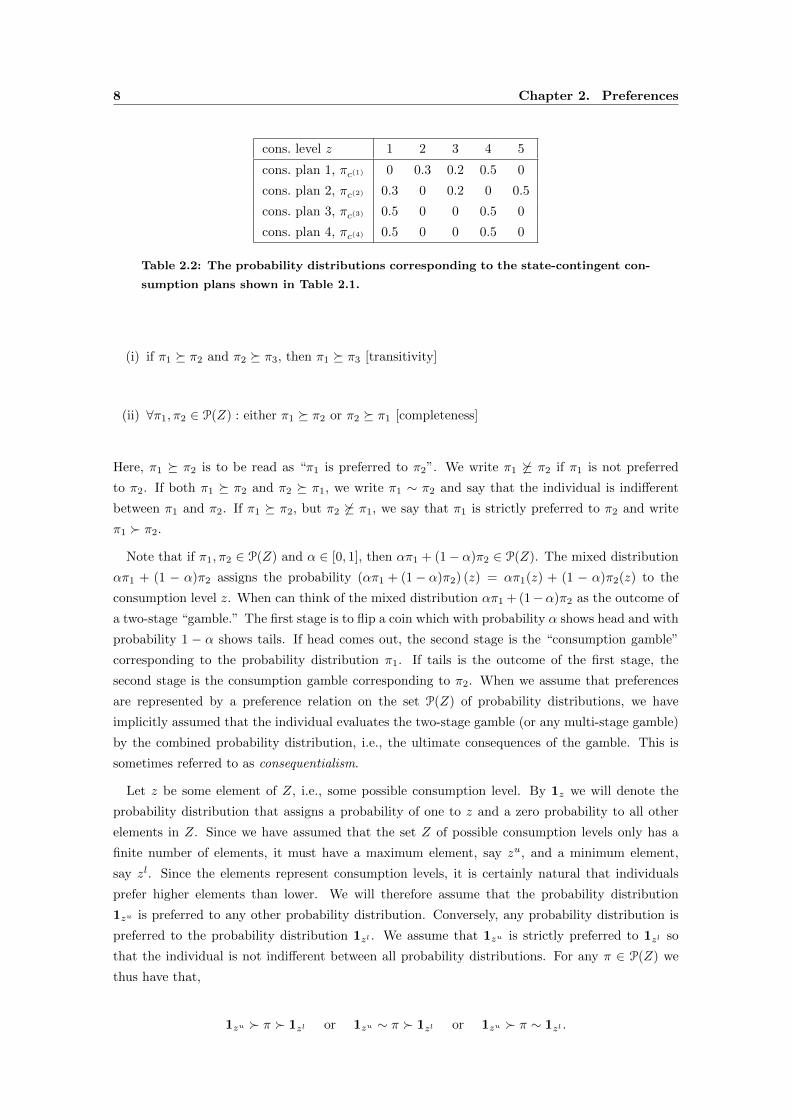
Table 2.1: The possible state-contingent consumption plans in the example.
plans generated by these choices. For example, she will be indifferent between two choices that
generate exactly the same consumption plans, i.e., the same consumption levels in all states. In
order to simplify the following analysis, we will assume a bit more, namely that the individual
only cares about the probability distribution of consumption generated by each portfolio. This is
effectively an assumption of state-independent preferences.
We can represent a consumption plan by a random variable c on (Ω,F,P). We assume that
there is only one consumption good and since consumption should be non-negative, c is valued in
R+ = [0,∞). As long as we are assuming a finite state space Ω = 1, 2, . . . , S we can equivalently
represent the consumption plan by a vector (c1, . . . , cS), where cω ∈ [0,∞) denotes the consumption
level if state ω is realized, i.e., cω ≡ c(ω). Let C denote the set of consumption plans that the
individual has to choose among. Let Z ⊆ R+ denote the set of all the possible levels of the
consumption plans that are considered, i.e., no matter which of these consumption plans we take,
its value will be in Z no matter which state is realized. Each consumption plan c ∈ C is associated
with a probability distribution πc, which is the function πc : Z → [0, 1], given by
πc(z) =∑
ω∈Ω: cω=z
pω,
i.e., the sum of the probabilities of those states in which the consumption level equals z.
As an example consider an economy with three possible states and four possible state-contingent
consumption plans as illustrated in Table 2.1. These four consumption plans may be the prod-
uct of four different portfolio choices. The set of possible end-of-period consumption levels is
Z = 1, 2, 3, 4, 5. Each consumption plan generates a probability distribution on the set Z. The
probability distributions corresponding to these consumption plans are as shown in Table 2.2. We
see that although the consumption plans c(3) and c(4) are different they generate identical proba-
bility distributions. By assumption individuals will be indifferent between these two consumption
plans.
Given these assumptions the individual will effectively choose between probability distributions
on the set of possible consumption levels Z. We assume for simplicity that Z is a finite set, but the
results can be generalized to the case of infinite Z at the cost of further mathematical complexity.
We denote by P(Z) the set of all probability distributions on Z that are generated by consumption
plans in C. A probability distribution π on the finite set Z is simply a function π : Z → [0, 1] with
the properties that∑z∈Z π(z) = 1 and π(A ∪B) = π(A) + π(B) whenever A ∩B = ∅.
We assume that the preferences of the individual can be represented by a preference relation on P(Z), which is a binary relation satisfying the following two conditions:
8 Chapter 2. Preferences
cons. level z 1 2 3 4 5
cons. plan 1, πc(1) 0 0.3 0.2 0.5 0
cons. plan 2, πc(2) 0.3 0 0.2 0 0.5
cons. plan 3, πc(3) 0.5 0 0 0.5 0
cons. plan 4, πc(4) 0.5 0 0 0.5 0
Table 2.2: The probability distributions corresponding to the state-contingent con-
sumption plans shown in Table 2.1.
(i) if π1 π2 and π2 π3, then π1 π3 [transitivity]
(ii) ∀π1, π2 ∈ P(Z) : either π1 π2 or π2 π1 [completeness]
Here, π1 π2 is to be read as “π1 is preferred to π2”. We write π1 6 π2 if π1 is not preferred
to π2. If both π1 π2 and π2 π1, we write π1 ∼ π2 and say that the individual is indifferent
between π1 and π2. If π1 π2, but π2 6 π1, we say that π1 is strictly preferred to π2 and write
π1 π2.
Note that if π1, π2 ∈ P(Z) and α ∈ [0, 1], then απ1 + (1− α)π2 ∈ P(Z). The mixed distribution
απ1 + (1 − α)π2 assigns the probability (απ1 + (1− α)π2) (z) = απ1(z) + (1 − α)π2(z) to the
consumption level z. When can think of the mixed distribution απ1 + (1−α)π2 as the outcome of
a two-stage “gamble.” The first stage is to flip a coin which with probability α shows head and with
probability 1 − α shows tails. If head comes out, the second stage is the “consumption gamble”
corresponding to the probability distribution π1. If tails is the outcome of the first stage, the
second stage is the consumption gamble corresponding to π2. When we assume that preferences
are represented by a preference relation on the set P(Z) of probability distributions, we have
implicitly assumed that the individual evaluates the two-stage gamble (or any multi-stage gamble)
by the combined probability distribution, i.e., the ultimate consequences of the gamble. This is
sometimes referred to as consequentialism.
Let z be some element of Z, i.e., some possible consumption level. By 1z we will denote the
probability distribution that assigns a probability of one to z and a zero probability to all other
elements in Z. Since we have assumed that the set Z of possible consumption levels only has a
finite number of elements, it must have a maximum element, say zu, and a minimum element,
say zl. Since the elements represent consumption levels, it is certainly natural that individuals
prefer higher elements than lower. We will therefore assume that the probability distribution
1zu is preferred to any other probability distribution. Conversely, any probability distribution is
preferred to the probability distribution 1zl . We assume that 1zu is strictly preferred to 1zl so
that the individual is not indifferent between all probability distributions. For any π ∈ P(Z) we
thus have that,
1zu π 1zl or 1zu ∼ π 1zl or 1zu π ∼ 1zl .

2.3 Utility indices 9
2.3 Utility indices
A utility index for a given preference relation is a function U : P(Z) → R that to each
probability distribution over consumption levels attaches a real-valued number such that
π1 π2 ⇔ U(π1) ≥ U(π2).
Note that a utility index is only unique up to a strictly increasing transformation. If U is a utility
index and f : R → R is any strictly increasing function, then the composite function V = f U,
defined by V(π) = f (U(π)), is also a utility index for the same preference relation.
We will show below that a utility index exists under the following two axiomatic assumptions
on the preference relation :
Axiom 2.1 (Monotonicity). Suppose that π1, π2 ∈ P(Z) with π1 π2 and let a, b ∈ [0, 1]. The
preference relation has the property that
a > b ⇔ aπ1 + (1− a)π2 bπ1 + (1− b)π2.
This is certainly a very natural assumption on preferences. If you consider a weighted average
of two probability distributions, you will prefer a high weight on the best of the two distributions.
Axiom 2.2 (Archimedean). The preference relation has the property that for any three proba-
bility distributions π1, π2, π3 ∈ P(Z) with π1 π2 π3, numbers a, b ∈ (0, 1) exist such that
aπ1 + (1− a)π3 π2 bπ1 + (1− b)π3.
The axiom basically says that no matter how good a probability distribution π1 is, it is so that
for any π2 π3 we can find some mixed distribution of π1 and π3 to which π2 is preferred. We just
have to put a sufficiently low weight on π1 in the mixed distribution. Similarly, no matter how bad
a probability distribution π3 is, it is so that for any π1 π2 we can find some mixed distribution
of π1 and π3 that is preferred to π2. We just have to put a sufficiently low weight on π3 in the
mixed distribution.
We shall say that a preference relation has the continuity property if for any three probability
distributions π1, π2, π3 ∈ P(Z) with π1 π2 π3, a unique number α ∈ (0, 1) exists such that
π2 ∼ απ1 + (1− α)π3.
We can easily extend this to the case where either π1 ∼ π2 or π2 ∼ π3. For π1 ∼ π2 π3,
π2 ∼ 1π1 +(1−1)π3 corresponding to α = 1. For π1 π2 ∼ π3, π2 ∼ 0π1 +(1−0)π3 corresponding
to α = 0. In words the continuity property means that for any three probability distributions there
is a unique combination of the best and the worst distribution so that the individual is indifferent
between the third “middle” distribution and this combination of the other two. This appears
to be closely related to the Archimedean Axiom and, in fact, the next lemma shows that the
Monotonicity Axiom and the Archimedean Axiom imply continuity of preferences.
Lemma 2.1. Let be a preference relation satisfying the Monotonicity Axiom and the Archimedean
Axiom. Then it has the continuity property.
Proof. Given π1 π2 π3. Define the number α by
α = supk ∈ [0, 1] | π2 kπ1 + (1− k)π3.

10 Chapter 2. Preferences
By the Monotonicity Axiom we have that π2 kπ1 + (1 − k)π3 for all k < α and that kπ1 +
(1 − k)π3 π2 for all k > α. We want to show that π2 ∼ απ1 + (1 − α)π3. Note that by the
Archimedean Axiom, there is some k > 0 such that π2 kπ1 + (1 − k)π3 and some k < 1 such
that kπ1 + (1− k)π3 π2. Consequently, α is in the open interval (0, 1).
Suppose that π2 απ1 + (1 − α)π3. Then according to the Archimedean Axiom we can find
a number b ∈ (0, 1) such that π2 bπ1 + (1 − b)απ1 + (1 − α)π3. The mixed distribution on
the right-hand side has a total weight of k = b + (1 − b)α = α + (1 − α)b > α on π1. Hence we
have found some k > α for which π2 kπ1 + (1 − k)π3. This contradicts the definition of α.
Consequently, we must have that π2 6 απ1 + (1− α)π3.
Now suppose that απ1 + (1 − α)π3 π2. Then we know from the Archimedean Axiom that a
number a ∈ (0, 1) exists such that aαπ1 + (1 − α)π3 + (1 − a)π3 π2. The mixed distribution
on the left-hand side has a total weight of aα < α on π1. Hence we have found some k < α for
which kπ1 + (1− k)π3 π2. This contradicts the definition of α. We can therefore also conclude
that απ1 + (1− α)π3 6 π2. In sum, we have π2 ∼ απ1 + (1− α)π3.
The next result states that a preference relation which satisfies the Monotonicity Axiom and
has the continuity property can always be represented by a utility index. In particular this is true
when satisfies the Monotonicity Axiom and the Archimedean Axiom.
Theorem 2.1. Let be a preference relation which satisfies the Monotonicity Axiom and has the
continuity property. Then it can be represented by a utility index U, i.e., a function U : P(Z)→ Rwith the property that
π1 π2 ⇔ U(π1) ≥ U(π2).
Proof. Recall that we have assumed a best probability distribution 1zu and a worst probability
distribution 1zl in the sense that
1zu π 1zl or 1zu ∼ π 1zl or 1zu π ∼ 1zl
for any π ∈ P(Z). For any π ∈ P(Z) we know from the continuity property that a unique number
απ ∈ [0, 1] exists such that
π ∼ απ1zu + (1− απ)1zl .
If 1zu ∼ π 1zl , απ = 1. If 1zu π ∼ 1zl , απ = 0. If 1zu π 1zl , απ ∈ (0, 1).
We define the function U : P(Z)→ R by U(π) = απ. By the Monotonicity Axiom we know that
U(π1) ≥ U(π2) if and only if
U(π1)1zu + (1− U(π1)) 1zl U(π2)1zu + (1− U(π2)) 1zl ,
and hence if and only if π1 π2. It follows that U is a utility index.
2.4 Expected utility representation of preferences
Utility indices are functions of probability distributions on the set of possible consumption
levels. With many states of the world and many assets to trade in, the set of such probability
distributions will be very, very large. This will significantly complicate the analysis of optimal
choice using utility indices to represent preferences. To simplify the analysis financial economists

2.4 Expected utility representation of preferences 11
traditionally put more structure on the preferences so that they can be represented in terms of
expected utility.
We say that a preference relation on P(Z) has an expected utility representation if there exists
a function u : Z → R such that
π1 π2 ⇔∑z∈Z
π1(z)u(z) ≥∑z∈Z
π2(z)u(z). (2.1)
Here∑z∈Z π(z)u(z) is the expected utility of end-of-period consumption given the consumption
probability distribution π, so (2.1) says that E[u(c1)] ≥ E[u(c2)], where ci is the random variable
representing end-of-period consumption with associated consumption probability distribution πi.
The function u is called a von Neumann-Morgenstern utility function or simply a utility function.
Note that u is defined on the set Z of consumption levels, which in general has a simpler structure
than the set of probability distributions on Z. Given a utility function u, we can obviously define
a utility index by U(π) =∑z∈Z π(z)u(z).
2.4.1 Conditions for expected utility
When can we use an expected utility representation of a preference relation? The next lemma
is a first step.
Lemma 2.2. A preference relation has an expected utility representation if and only if it can
be represented by a linear utility index U in the sense that
U (aπ1 + (1− a)π2) = aU(π1) + (1− a)U(π2)
for any π1, π2 ∈ P(Z) and any a ∈ [0, 1].
Proof. Suppose that has an expected utility representation with utility function u. Define
U : P(Z) → R by U(π) =∑z∈Z π(z)u(z). Then clearly U is a utility index representing and U
is linear since
U (aπ1 + (1− a)π2) =∑z∈Z
(aπ1(z) + (1− a)π2(z))u(z)
= a∑z∈Z
π1(z)u(z) + (1− a)∑z∈Z
π2(z)u(z)
= aU(π1) + (1− a)U(π2).
Conversely, suppose that U is a linear utility index representing . Define a function u : Z → Rby u(z) = U(1z). For any π ∈ P(Z) we have
π ∼∑z∈Z
π(z)1z.
Therefore,
U(π) = U
(∑z∈Z
π(z)1z
)=∑z∈Z
π(z)U(1z) =∑z∈Z
π(z)u(z).
Since U is a utility index, we have π1 π2 ⇔ U(π1) ≥ U(π2), which the computation above shows
is equivalent to∑z∈Z π1(z)u(z) ≥
∑z∈Z π2(z)u(z). Consequently, u gives an expected utility
representation of .

12 Chapter 2. Preferences
z 1 2 3 4
π1 0 0.2 0.6 0.2
π2 0 0.4 0.2 0.4
π3 1 0 0 0
π4 0.5 0.1 0.3 0.1
π5 0.5 0.2 0.1 0.2
Table 2.3: The probability distributions used in the illustration of the Substitution
Axiom.
The question then is under what assumptions the preference relation can be represented by
a linear utility index. As shown by von Neumann and Morgenstern (1944) we need an additional
axiom, the so-called Substitution Axiom.
Axiom 2.3 (Substitution). For all π1, π2, π3 ∈ P(Z) and all a ∈ (0, 1], we have
π1 π2 ⇔ aπ1 + (1− a)π3 aπ2 + (1− a)π3
and
π1 ∼ π2 ⇔ aπ1 + (1− a)π3 ∼ aπ2 + (1− a)π3.
The Substitution Axiom is sometimes called the Independence Axiom or the Axiom of the
Irrelevance of the Common Alternative. Basically, it says that when the individual is to compare
two probability distributions, she needs only consider the parts of the two distributions which
are different from each other. As an example, suppose the possible consumption levels are Z =
1, 2, 3, 4 and consider the probability distributions on Z given in Table 2.3. Suppose you want
to compare the distributions π4 and π5. They only differ in the probabilities they associate with
consumption levels 2, 3, and 4 so it should only be necessary to focus on these parts. More formally
observe that
π4 ∼ 0.5π1 + 0.5π3 and π5 ∼ 0.5π2 + 0.5π3.
π1 is the conditional distribution of π4 given that the consumption level is different from 1 and
π2 is the conditional distribution of π5 given that the consumption level is different from 1. The
Substitution Axiom then says that
π4 π5 ⇔ π1 π2.
The next lemma shows that the Substitution Axiom is more restrictive than the Monotonicity
Axiom.
Lemma 2.3. If a preference relation satisfies the Substitution Axiom, it will also satisfy the
Monotonicity Axiom.
Proof. Given π1, π2 ∈ P(Z) with π1 π2 and numbers a, b ∈ [0, 1]. We have to show that
a > b ⇔ aπ1 + (1− a)π2 bπ1 + (1− b)π2.
Note that if a = 0, we cannot have a > b, and if aπ1 + (1− a)π2 bπ1 + (1− b)π2 we cannot have
a = 0. We can therefore safely assume that a > 0.

2.4 Expected utility representation of preferences 13
First assume that a > b. Observe that it follows from the Substitution Axiom that
aπ1 + (1− a)π2 aπ2 + (1− a)π2
and hence that aπ1 + (1 − a)π2 π2. Also from the Substitution Axiom we have that for any
π3 π2, we have
π3 ∼(
1− b
a
)π3 +
b
aπ3
(1− b
a
)π2 +
b
aπ3.
Due to our observation above, we can use this with π3 = aπ1 + (1− a)π2. Then we get
aπ1 + (1− a)π2 b
aaπ1 + (1− a)π2+
(1− b
a
)π2
∼ bπ1 + (1− b)π2,
as was to be shown.
Conversely, assuming that
aπ1 + (1− a)π2 bπ1 + (1− b)π2,
we must argue that a > b. The above inequality cannot be true if a = b since the two combined
distributions are then identical. If b was greater than a, we could follow the steps above with a and
b swapped and end up concluding that bπ1 + (1− b)π2 aπ1 + (1− a)π2, which would contradict
our assumption. Hence, we cannot have neither a = b nor a < b but must have a > b.
Next we state the main result:
Theorem 2.2. Assume that Z is finite and that is a preference relation on P(Z). Then can
be represented by a linear utility index if and only if satisfies the Archimedean Axiom and the
Substitution Axiom.
Proof. First suppose the preference relation satisfies the Archimedean Axiom and the Substi-
tution Axiom. Define a utility index U : P(Z) → R exactly as in the proof of Theorem 2.1, i.e.,
U(π) = απ, where απ ∈ [0, 1] is the unique number such that
π ∼ απ1zu + (1− απ)1zl .
We want to show that, as a consequence of the Substitution Axiom, U is indeed linear. For that
purpose, pick any two probability distributions π1, π2 ∈ P(Z) and any number a ∈ [0, 1]. We want
to show that U (aπ1 + (1− a)π2) = aU(π1) + (1− a)U(π2). We can do that by showing that
aπ1 + (1− a)π2 ∼ (aU(π1) + (1− a)U(π2)) 1zu + (1− aU(π1) + (1− a)U(π2)) 1zl .
This follows from the Substitution Axiom:
aπ1 + (1− a)π2 ∼ aU(π1)1zu + (1− U(π1)) 1zl+ (1− a)U(π2)1zu + (1− U(π2)) 1zl
∼ (aU(π1) + (1− a)U(π2)) 1zu + (1− aU(π1) + (1− a)U(π2)) 1zl .
Now let us show the converse, i.e., if can be represented by a linear utility index U, then it must
satisfy the Archimedean Axiom and the Substitution Axiom. In order to show the Archimedean
14 Chapter 2. Preferences
Axiom, we pick π1 π2 π3, which means that U(π1) > U(π2) > U(π3), and must find numbers
a, b ∈ (0, 1) such that
aπ1 + (1− a)π3 π2 bπ1 + (1− b)π3,
i.e., that
U (aπ1 + (1− a)π3) > U(π2) > U (bπ1 + (1− b)π3) .
Define the number a by
a = 1− 1
2
U(π1)− U(π2)
U(π1)− U(π3).
Then a ∈ (0, 1) and by linearity of U we get
U (aπ1 + (1− a)π3) = aU(π1) + (1− a)U(π3)
= U(π1) + (1− a) (U(π3)− U(π1))
= U(π1)− 1
2(U(π1)− U(π2))
=1
2(U(π1) + U(π2))
> U(π2).
Similarly for b.
In order to show the Substitution Axiom, we take π1, π2, π3 ∈ P(Z) and any number a ∈ (0, 1].
We must show that π1 π2 if and only if aπ1 + (1− a)π3 aπ2 + (1− a)π3, i.e.,
U(π1) > U(π2) ⇔ U (aπ1 + (1− a)π3) > U (aπ2 + (1− a)π3) .
This follows immediately by linearity of U:
U (aπ1 + (1− a)π3) = aU(π1) + U ((1− a)π3)
> aU(π2) + U ((1− a)π3)
= U (aπ2 + (1− a)π3)
with the inequality holding if and only if U(π1) > U(π2). Similarly, we can show that π1 ∼ π2 if
and only if aπ1 + (1− a)π3 ∼ aπ2 + (1− a)π3.
The next theorem shows which utility functions that represent the same preference relation. The
proof is left for the reader as Exercise 2.1.
Theorem 2.3. A utility function for a given preference relation is only determined up to a strictly
increasing affine transformation, i.e., if u is a utility function for , then v will be so if and only
if there exist constants a > 0 and b such that v(z) = au(z) + b for all z ∈ Z.
If one utility function is an affine function of another, we will say that they are equivalent. Note
that an easy consequence of this theorem is that it does not really matter whether the utility is
positive or negative. At first, you might find negative utility strange but we can always add a
sufficiently large positive constant without affecting the ranking of different consumption plans.
Suppose U is a utility index with an associated utility function u. If f is any strictly increasing
transformation, then V = f U is also a utility index for the same preferences, but f u is only
the utility function for V if f is affine.

2.4 Expected utility representation of preferences 15
The expected utility associated with a probability distribution π on Z is∑z∈Z π(z)u(z). Recall
that the probability distributions we consider correspond to consumption plans. Given a con-
sumption plan, i.e., a random variable c, the associated probability distribution is defined by the
probabilities
π(z) = P (ω ∈ Ω|c(ω) = z) =∑
ω∈Ω:c(ω)=z
pω.
The expected utility associated with the consumption plan c is therefore
E[u(c)] =∑ω∈Ω
pωu(c(ω)) =∑z∈Z
∑ω∈Ω:c(ω)=z
pωu(z) =∑z∈Z
π(z)u(z).
Of course, if c is a risk-free consumption plan in the sense that a z exists such that c(ω) = z for all
ω, then the expected utility is E[u(c)] = u(z). With a slight abuse of notation we will just write
this as u(c).
2.4.2 Some technical issues
Infinite Z. What if Z is infinite, e.g., Z = R+ ≡ [0,∞)? It can be shown that in this case a
preference relation has an expected utility representation if the Archimedean Axiom, the Substi-
tution Axiom, an additional axiom (“the sure thing principle”), and “some technical conditions”
are satisfied. Fishburn (1970) gives the details.
Expected utility in this case: E[u(c)] =∫Zu(z)π(z) dz, where π is a probability density function
derived from the consumption plan c.
Boundedness of expected utility. Suppose u is unbounded from above and R+ ⊆ Z. Then
there exists (zn)∞n=1 ⊆ Z with zn → ∞ and u(zn) ≥ 2n. Expected utility of consumption plan π1
with π1(zn) = 1/2n:∞∑n=1
u(zn)π1(zn) ≥∞∑n=1
2n1
2n=∞.
If π2, π3 are such that π1 π2 π3, then the expected utility of π2 and π3 must be finite. But
for no b ∈ (0, 1) do we have
π2 bπ1 + (1− b)π3 [expected utility =∞].
• no problem if Z is finite
• no problem if R+ ⊆ Z, u is concave, and consumption plans have finite expectations:
u concave ⇒ u is differentiable in some point b and
u(z) ≤ u(b) + u′(b)(z − b), ∀z ∈ Z.
If the consumption plan c has finite expectations, then
E[u(c)] ≤ E[u(b) + u′(b)(c− b)] = u(b) + u′(b) (E[c]− b) <∞.

16 Chapter 2. Preferences
z 0 1 5
π1 0 1 0
π2 0.01 0.89 0.1
π3 0.9 0 0.1
π4 0.89 0.11 0
Table 2.4: The probability distributions used in the illustration of the Allais Para-
dox.
Subjective probability. We have taken the probabilities of the states of nature as exogenously
given, i.e., as objective probabilities. However, in real life individuals often have to form their own
probabilities about many events, i.e., they form subjective probabilities. Although the analysis is
a bit more complicated, Savage (1954) and Anscombe and Aumann (1963) show that the results
we developed above carry over to the case of subjective probabilities. For an introduction to this
analysis, see Kreps (1990, Ch. 3).
2.4.3 Are the axioms reasonable?
The validity of the Substitution Axiom, which is necessary for obtaining the expected utility
representation, has been intensively discussed in the literature. Some researchers have conducted
experiments in which the decisions made by the participating individuals conflict with the Substi-
tution Axiom.
The most famous challenge is the so-called Allais Paradox named after Allais (1953). Here is
one example of the paradox. Suppose Z = 0, 1, 5. Consider the consumption plans in Table 2.4.
The Substitution Axiom implies that π1 π2 ⇒ π4 π3. This can be seen from the following:
0.11($1) + 0.89 ($1) ∼ π1 π2 ∼ 0.11
(1
11($0) +
10
11($5)
)+ 0.89 ($1) ⇒
0.11($1) + 0.89 ($0)︸ ︷︷ ︸π4∼
0.11
(1
11($0) +
10
11($5)
)+ 0.89 ($0) ∼ 0.9($0) + 0.1($5)︸ ︷︷ ︸
π3∼
Nevertheless individuals preferring π1 to π2 often choose π3 over π4. Apparently people tend to
over-weight small probability events, e.g., ($0) in π2.
Other “problems”:
• the “framing” of possible choices, i.e., the way you get the alternatives presented, seem to
affect decisions
• models assume individuals have unlimited rationality
2.5 Risk aversion
In this section we focus on the attitudes towards risk reflected by the preferences of an individual.
We assume that the preferences can be represented by a utility function u and that u is strictly
increasing so that the individual is “greedy,” i.e., prefers high consumption to low consumption.
We assume that the utility function is defined on some interval Z of R, e.g., Z = R+ ≡ [0,∞).

2.5 Risk aversion 17
2.5.1 Risk attitudes
Fix a consumption level c ∈ Z. Consider a random variable ε with E[ε] = 0. We can think of
c+ ε as a random variable representing a consumption plan with consumption c+ ε(ω) if state ω
is realized. Note that E[c+ ε] = c. Such a random variable ε is called a fair gamble or a zero-mean
risk.
An individual is said to be (strictly) risk-averse if she for all c ∈ Z and all fair gambles ε
(strictly) prefers the sure consumption level c to c + ε. In other words, a risk-averse individual
rejects all fair gambles. Similarly, an individual is said to be (strictly) risk-loving if she for all
c ∈ Z (strictly) prefers c + ε to c, and said to be risk-neutral if she for all c ∈ Z is indifferent
between accepting any fair gamble or not. Of course, individuals may be neither risk-averse, risk-
neutral, or risk-loving, for example if they reject fair gambles around some values of c and accept
fair gambles around other values of c. Individuals may be locally risk-averse, locally risk-neutral,
and locally risk-loving. Since it is generally believed that individuals are risk-averse, we focus on
preferences exhibiting that feature.
We can think of any consumption plan c as the sum of its expected value E[c] and a fair gamble
ε = c−E[c]. It follows that an individual is risk-averse if she prefers the sure consumption E[c] to
the random consumption c, i.e., if u(E[c]) ≥ E[u(c)]. By Jensen’s Inequality, this is true exactly
when u is a concave function and the strict inequality holds if u is strictly concave and c is a
non-degenerate random variable, i.e., it does not have the same value in all states. Recall that
u : Z → R concave means that for all z1, z2 ∈ Z and all a ∈ (0, 1) we have
u (az1 + (1− a)z2) ≥ au(z1) + (1− a)u(z2).
If the strict inequality holds in all cases, the function is said to be strictly concave. By the above
argument, we have the following theorem:
Theorem 2.4. An individual with a utility function u is (strictly) risk-averse if and only if u is
(strictly) concave.
Similarly, an individual is (strictly) risk-loving if and only if the utility function is (strictly)
convex. An individual is risk-neutral if and only if the utility function is affine.
2.5.2 Quantitative measures of risk aversion
We will focus on utility functions that are continuous and twice differentiable on the interior
of Z. By our assumption of greedy individuals, we then have u′ > 0, and the concavity of the
utility function for risk-averse investors is then equivalent to u′′ ≤ 0.
The certainty equivalent of the random consumption plan c is defined as the c∗ ∈ Z such that
u(c∗) = E[u(c)],
i.e., the individual is just as satisfied getting the consumption level c∗ for sure as getting the random
consumption c. With Z ⊆ R, c∗ uniquely exists due to our assumptions that u is continuous and
strictly increasing. From the definition of the certainty equivalent it is clear that an individual will
rank consumption plans according to their certainty equivalents.

18 Chapter 2. Preferences
For a risk-averse individual we have the certainty equivalent c∗ of a consumption plan is smaller
than the expected consumption level E[c]. The risk premium associated with the consumption
plan c is defined as λ(c) = E[c]− c∗ so that
E[u(c)] = u(c∗) = u(E[c]− λ(c)).
The risk premium is the consumption the individual is willing to give up in order to eliminate the
uncertainty.
The degree of risk aversion is associated with u′′, but a good measure of risk aversion should be
invariant to strictly positive, affine transformations. This is satisfied by the Arrow-Pratt measures
of risk aversion defined as follows. The Absolute Risk Aversion is given by
ARA(c) = −u′′(c)
u′(c).
The Relative Risk Aversion is given by
RRA(c) = −cu′′(c)
u′(c)= cARA(c).
We can link the Arrow-Pratt measures to the risk premium in the following way. Let c ∈ Z
denote some fixed consumption level and let ε be a fair gamble. The resulting consumption plan
is then c = c+ ε. Denote the corresponding risk premium by λ(c, ε) so that
E[u(c+ ε)] = u(c∗) = u (c− λ(c, ε)) . (2.2)
We can approximate the left-hand side of (2.2) by
E[u(c+ ε)] ≈ E
[u(c) + εu′(c) +
1
2ε2u′′(c)
]= u(c) +
1
2Var[ε]u′′(c),
using E[ε] = 0 and Var[ε] = E[ε2] − E[ε]2 = E[ε2], and we can approximate the right-hand side
of (2.2) by
u (c− λ(c, ε)) ≈ u(c)− λ(c, ε)u′(c).
Hence we can write the risk premium as
λ(c, ε) ≈ −1
2Var[ε]
u′′(c)
u′(c)=
1
2Var[ε] ARA(c).
Of course, the approximation is more accurate for “small” gambles. Thus the risk premium for a
small fair gamble around c is roughly proportional to the absolute risk aversion at c. We see that
the absolute risk aversion ARA(c) is constant if and only if λ(c, ε) is independent of c.
Loosely speaking, the absolute risk aversion ARA(c) measures the aversion to a fair gamble of
a given dollar amount around c, such as a gamble where there is an equal probability of winning
or loosing 1000 dollars. Since we expect that a wealthy investor will be less averse to that gamble
than a poor investor, the absolute risk aversion is expected to be a decreasing function of wealth.
Note that
ARA′(c) = −u′′′(c)u′(c)− u′′(c)2
u′(c)2=
(u′′(c)
u′(c)
)2
− u′′′(c)
u′(c)< 0 ⇒ u′′′(c) > 0,
that is, a positive third-order derivative of u is necessary for the utility function u to exhibit
decreasing absolute risk aversion.

2.5 Risk aversion 19
Now consider a “multiplicative” fair gamble around c in the sense that the resulting consumption
plan is c = c (1 + ε) = c+ cε, where E[ε] = 0. The risk premium is then
λ(c, cε) ≈ 1
2Var[cε] ARA(c) =
1
2c2 Var[ε] ARA(c) =
1
2cVar[ε] RRA(c)
implying thatλ(c, cε)
c≈ 1
2Var[ε] RRA(c). (2.3)
The fraction of consumption you require to engage in the multiplicative risk is thus (roughly) pro-
portional to the relative risk aversion at c. Note that utility functions with constant or decreasing
(or even modestly increasing) relative risk aversion will display decreasing absolute risk aversion.
Some authors use terms like risk tolerance and risk cautiousness. The absolute risk tolerance
at c is simply the reciprocal of the absolute risk aversion, i.e.,
ART(c) =1
ARA(c)= − u
′(c)
u′′(c).
Similarly, the relative risk tolerance is the reciprocal of the relative risk aversion. The risk cau-
tiousness at c is defined as the rate of change in the absolute risk tolerance, i.e., ART′(c).
2.5.3 Comparison of risk aversion between individuals
An individual with utility function u is said to be more risk-averse than an individual with
utility function v if for any consumption plan c and any fixed c ∈ Z with E[u(c)] ≥ u(c), we have
E[v(c)] ≥ v(c). So the v-individual will accept all gambles that the u-individual will accept – and
possibly some more. Pratt (1964) has shown the following theorem:
Theorem 2.5. Suppose u and v are twice continuously differentiable and strictly increasing. Then
the following conditions are equivalent:
(a) u is more risk-averse than v,
(b) ARAu(c) ≥ ARAv(c) for all c ∈ Z,
(c) a strictly increasing and concave function f exists such that u = f v.
Proof. First let us show (a) ⇒ (b): Suppose u is more risk-averse than v, but that ARAu(c) <
ARAv(c) for some c ∈ Z. Since ARAu and ARAv are continuous, we must then have that
ARAu(c) < ARAv(c) for all c in an interval around c. Then we can surely find a small gamble
around c, which the u-individual will accept, but the v-individual will reject. This contradicts the
assumption in (a).
Next, we show (b) ⇒ (c): Since v is strictly increasing, it has an inverse v−1 and we can define
a function f by f(x) = u(v−1(x)
). Then clearly f(v(c)) = u(c) so that u = f v. The first-order
derivative of f is
f ′(x) =u′(v−1(x)
)v′ (v−1(x))
,
which is positive since u and v are strictly increasing. Hence, f is strictly increasing. The second-
order derivative is
f ′′(x) =u′′(v−1(x)
)−v′′(v−1(x)
)u′(v−1(x)
)/v′(v−1(x)
)v′ (v−1(x))
2
=u′(v−1(x)
)v′ (v−1(x))
2
(ARAv
(v−1(x)
)−ARAu
(v−1(x)
)).

20 Chapter 2. Preferences
From (b), it follows that f ′′(x) < 0, hence f is concave.
Finally, we show that (c) ⇒ (a): assume that for some consumption plan c and some c ∈ Z, we
have E[u(c)] ≥ u(c) but E[v(c)] < v(c). We want to arrive at a contradiction.
f (v(c)) = u(c) ≤ E[u(c)] = E[f(v(c))]
< f (E[v(c)])
< f (v(c)) ,
where we use the concavity of f and Jensen’s Inequality to go from the first to the second line, and
we use that f is strictly increasing to go from the second to the third line. Now the contradiction
is clear.
2.6 Utility functions in models and in reality
2.6.1 Frequently applied utility functions
CRRA utility. (Also known as power utility or isoelastic utility.) Utility functions u(c) in this
class are defined for c ≥ 0:
u(c) =c1−γ
1− γ, (2.4)
where γ > 0 and γ 6= 1. Since
u′(c) = c−γ and u′′(c) = −γc−γ−1,
the absolute and relative risk aversions are given by
ARA(c) = −u′′(c)
u′(c)=γ
c, RRA(c) = cARA(c) = γ.
The relative risk aversion is constant across consumption levels c, hence the name CRRA (Constant
Relative Risk Aversion) utility. Note that u′(0+) ≡ limc→0 u′(c) = ∞ with the consequence that
an optimal solution will have the property that consumption/wealth c will be strictly above 0
with probability one. Hence, we can ignore the very appropriate non-negativity constraint on
consumption since the constraint will never be binding. Furthermore, u′(∞) ≡ limc→∞ u′(c) = 0.
Some authors assume a utility function of the form u(c) = c1−γ , which only makes sense for
γ ∈ (0, 1). However, empirical studies indicate that most investors have a relative risk aversion
above 1, cf. the discussion below. The absolute risk tolerance is linear in c:
ART(c) =1
ARA(c)=c
γ.
Except for a constant, the utility function
u(c) =c1−γ − 1
1− γ
is identical to the utility function specified in (2.4). The two utility functions are therefore equiv-
alent in the sense that they generate identical rankings of consumption plans and, in particular,
identical optimal choices. The advantage in using the latter definition is that this function has a
well-defined limit as γ → 1. From l’Hospital’s rule we have that
limγ→1
c1−γ − 1
1− γ= limγ→1
−c1−γ ln c
−1= ln c,

2.6 Utility functions in models and in reality 21
-6
-4
-2
0
2
4
6
0 4 8 12 16
RRA=0.5 RRA=1 RRA=2 RRA=5
Figure 2.1: Some CRRA utility functions.
which is the important special case of logarithmic utility. When we consider CRRA utility,
we will assume the simpler version (2.4), but we will use the fact that we can obtain the optimal
strategies of a log-utility investor as the limit of the optimal strategies of the general CRRA investor
as γ → 1.
Some CRRA utility functions are illustrated in Figure 2.1.
HARA utility. (Also known as extended power utility.) The absolute risk aversion for CRRA
utility is hyperbolic in c. More generally a utility function is said to be a HARA (Hyperbolic
Absolute Risk Aversion) utility function if
ARA(c) = −u′′(c)
u′(c)=
1
αc+ β
for some constants α, β such that αc + β > 0 for all relevant c. HARA utility functions are
sometimes referred to as affine (or linear) risk tolerance utility functions since the absolute risk
tolerance is
ART(c) =1
ARA(c)= αc+ β.
The risk cautiousness is ART′(c) = α.
How do the HARA utility functions look like? First, let us take the case α = 0, which implies
that the absolute risk aversion is constant (so-called CARA utility) and β must be positive.
d(lnu′(c))
dc=u′′(c)
u′(c)= − 1
β
implies that
lnu′(c) = − cβ
+ k1 ⇒ u′(c) = ek1e−c/β

22 Chapter 2. Preferences
for some constant k1. Hence,
u(c) = − 1
βek1e−c/β + k2
for some other constant k2. Applying the fact that increasing affine transformations do not change
decisions, the basic representative of this class of utility functions is the negative exponential
utility function
u(c) = −e−ac, c ∈ R,
where the parameter a = 1/β is the absolute risk aversion. Constant absolute risk aversion is
certainly not very reasonable. Nevertheless, the negative exponential utility function is sometimes
used for computational purposes in connection with normally distributed returns, e.g., in one-
period models.
Next, consider the case α 6= 0. Applying the same procedure as above we find
d(lnu′(c))
dc=u′′(c)
u′(c)= − 1
αc+ β⇒ lnu′(c) = − 1
αln(αc+ β) + k1
so that
u′(c) = ek1 exp
− 1
αln(αc+ β)
= ek1 (αc+ β)
−1/α. (2.5)
For α = 1 this implies that
u(c) = ek1 ln(c+ β) + k2.
The basic representative of such utility functions is the extended log utility function
u(c) = ln (c− c) , c > c,
where we have replaced β by −c. For α 6= 1, Equation (2.5) implies that
u(c) =1
αek1
1
1− 1α
(αc+ β)1−1/α
+ k2.
For α < 0, we can write the basic representative is
u(c) = − (c− c)1−γ, c < c,
where γ = 1/α < 0. We can think of c as a satiation level and call this subclass satiation HARA
utility functions. The absolute risk aversion is
ARA(c) =−γc− c
,
which is increasing in c, conflicting with intuition and empirical studies. Some older financial
models used the quadratic utility function, which is the special case with γ = −1 so that u(c) =
− (c− c)2. An equivalent utility function is u(c) = c− ac2.
For α > 0 (and α 6= 1), the basic representative is
u(c) =(c− c)1−γ
1− γ, c > c,
where γ = 1/α > 0. The limit as γ → 1 of the equivalent utility function (c−c)1−γ−11−γ is equal to the
extended log utility function u(c) = ln(c− c). We can think of c as a subsistence level of wealth or
2.6 Utility functions in models and in reality 23
consumption (which makes sense only if c ≥ 0) and refer to this subclass as subsistence HARA
utility functions. The absolute and relative risk aversions are
ARA(c) =γ
c− c, RRA(c) =
γc
c− c=
γ
1− (c/c),
which are both decreasing in c. The relative risk aversion approaches ∞ for c → c and decreases
to the constant γ for c→∞. Clearly, for c = 0, we are back to the CRRA utility functions so that
these also belong to the HARA family.
Mean-variance preferences. For some problems it is convenient to assume that the expected
utility associated with an uncertain consumption plan only depends on the expected value and the
variance of the consumption plan. This is certainly true if the consumption plan is a normally
distributed random variable since its probability distribution is fully characterized by the mean and
variance. However, it is generally not appropriate to use a normal distribution for consumption
(or wealth or asset returns).
For a quadratic utility function, u(c) = c− ac2, the expected utility is
E[u(c)] = E[c− ac2
]= E[c]− aE
[c2]
= E[c]− a(Var[c] + E[c]2
),
which is indeed a function of the expected value and the variance of the consumption plan. Alas,
the quadratic utility function is inappropriate for several reasons. Most importantly, it exhibits
increasing absolute risk aversion.
For a general utility function the expected utility of a consumption plan will depend on all
moments. This can be seen by the Taylor expansion of u(c) around the expected consumption,
E[c]:
u(c) = u(E[c]) + u′(E[c])(c− E[c]) +1
2u′′(E[c])(c− E[c])2 +
∞∑n=3
1
n!u(n)(E[c])(c− E[c])n,
where u(n) is the n’th derivative of u. Taking expectations, we get
E[u(c)] = u(E[c]) +1
2u′′(E[c]) Var[c] +
∞∑n=3
1
n!u(n)(E[c]) E [(c− E[c])n] .
Here E [(c− E[c])n] is the central moment of order n. The variance is the central moment of order 2.
Obviously, a greedy investor (which just means that u is increasing) will prefer higher expected
consumption to lower for fixed central moments of order 2 and higher. Moreover, a risk-averse
investor (so that u′′ < 0) will prefer lower variance of consumption to higher for fixed expected
consumption and fixed central moments of order 3 and higher. But when the central moments
of order 3 and higher are not the same for all alternatives, we cannot just evaluate them on the
basis of their expectation and variance. With quadratic utility, the derivatives of u of order 3
and higher are zero so there it works. In general, mean-variance preferences can only serve as an
approximation of the true utility function.
2.6.2 What do we know about individuals’ risk aversion?
From our discussion of risk aversion and various utility functions we expect that individuals are
risk averse and exhibit decreasing absolute risk aversion. But can this be supported by empirical

24 Chapter 2. Preferences
evidence? Do individuals have constant relative risk aversion? And what is a reasonable level of
risk aversion for individuals?
You can get an idea of the risk attitudes of an individual by observing how they choose between
risky alternatives. Some researchers have studied this by setting up “laboratory experiments” in
which they present some risky alternatives to a group of individuals and simply see what they
prefer. Some of these experiments suggest that expected utility theory is frequently violated,
see e.g., Grether and Plott (1979). However, laboratory experiments are problematic for several
reasons. You cannot be sure that individuals will make the same choice in what they know is an
experiment as they would in real life. It is also hard to formulate alternatives that resemble the
rather complex real-life decisions. It seems more fruitful to study actual data on how individuals
have acted confronted with real-life decision problems under uncertainty. A number of studies do
that.
Friend and Blume (1975) analyze data on household asset holdings. They conclude that the
data is consistent with individuals having roughly constant relative risk aversion and that the
coefficients of relative risk aversion are “on average well in excess of one and probably in excess of
two” (quote from page 900 in their paper). Pindyck (1988) finds support of a relative risk aversion
between 3 and 4 in a structural model of the reaction of stock prices to fundamental variables.
Other studies are based on insurance data. Using U.S. data on so-called property/liability
insurance, Szpiro (1986) finds support of CRRA utility with a relative risk aversion coefficient
between 1.2 and 1.8. Cicchetti and Dubin (1994) work with data from the U.S. on whether
individuals purchased an insurance against the risk of trouble with their home telephone line.
They conclude that the data is consistent with expected utility theory and that a subsistence
HARA utility function performs better than log utility or negative exponential utility.
Ogaki and Zhang (2001) study data on individual food consumption from Pakistan and India
and conclude that relative risk aversion is decreasing for poor individuals, which is consistent with
a subsistence HARA utility function.
It is an empirical fact that even though consumption and wealth have increased tremendously
over the years, the magnitude of real rates of return has not changed dramatically. As indicated
by (2.3) relative risk premia are approximately proportional to the relative risk aversion. As
discussed in, e.g., Munk (2012), basic asset pricing theory implies that relative risk premia on
financial assets (in terms of expected real return in excess of the real risk-free return) will be
proportional to the “average” relative risk aversion in the economy. If the “average” relative risk
aversion was significantly decreasing (increasing) in the level of consumption or wealth, we should
have seen decreasing (increasing) real returns on risky assets in the past. The data seems to be
consistent with individuals having “on average” close to CRRA utility.
To get a feeling of what a given risk aversion really means, suppose you are confronted with
two consumption plans. One plan is a sure consumption of c, the other plan gives you (1 − α)c
with probability 0.5 and (1 + α)c with probability 0.5. If you have a CRRA utility function
u(c) = c1−γ/(1− γ), the certainty equivalent c∗ of the risky plan is determined by
1
1− γ(c∗)
1−γ=
1
2
1
1− γ((1− α)c)
1−γ+
1
2
1
1− γ((1 + α)c)
1−γ,

2.6 Utility functions in models and in reality 25
γ = RRA α = 1% α = 10% α = 50%
0.5 0.00% 0.25% 6.70%
1 0.01% 0.50% 13.40%
2 0.01% 1.00% 25.00%
5 0.02% 2.43% 40.72%
10 0.05% 4.42% 46.00%
20 0.10% 6.76% 48.14%
50 0.24% 8.72% 49.29%
100 0.43% 9.37% 49.65%
Table 2.5: Relative risk premia for a fair gamble of the fraction α of your consump-
tion.
which implies that
c∗ =
(1
2
)1/(1−γ) [(1− α)1−γ + (1 + α)1−γ]1/(1−γ)
c.
The risk premium λ(c, α) is
λ(c, α) = c− c∗ =
(1−
(1
2
)1/(1−γ) [(1− α)1−γ + (1 + α)1−γ]1/(1−γ)
)c.
Both the certainty equivalent and the risk premium are thus proportional to the consumption
level c. The relative risk premium λ(c, α)/c is simply one minus the relative certainty equivalent
c∗/c. These equations assume γ 6= 1. In Exercise 2.5 you are asked to find the certainty equivalent
and risk premium for log-utility corresponding to γ = 1.
Table 2.5 shows the relative risk premium for various values of the relative risk aversion coefficient
γ and various values of α, the “size” of the risk. For example, an individual with γ = 5 is willing to
sacrifice 2.43% of the safe consumption in order to avoid a fair gamble of 10% of that consumption
level. Of course, even extremely risk averse individuals will not sacrifice more than they can loose
but in some cases it is pretty close. Looking at these numbers, it is hard to believe in γ-values
outside, say, [1, 10]. In Exercise 2.6 you are asked to compare the exact relative risk premia shown
in the table with the approximate risk premia given by (2.3).
2.6.3 Two-good utility functions and the elasticity of substitution
Consider an atemporal utility function f(c, z) of two consumption of two different goods at
the same time. An indifference curve in the (c, z)-space is characterized by f(c, z) = k for some
constant k. Changes in c and z along an indifference curve are linked by
∂f
∂cdc+
∂f
∂zdz = 0
so that the slope of the indifference curve (also known as the marginal rate of substitution) is
dz
dc= −
∂f∂c∂f∂z
.

26 Chapter 2. Preferences
Unless the indifference curve is linear, its slope will change along the curve. Indifference curves are
generally assumed to be convex. The elasticity of substitution tells you by which percentage you
need to change z/c in order to obtain a one percent change in the slope of the indifference curve. It
is a measure of the curvature or convexity of the indifference curve. If the indifference curve is very
curved, you only have to move a little along the curve before its slope has changed by one percent.
Hence, the elasticity of substitution is low. If the indifference curve is almost linear, you have to
move far away to change the slope by one percent. In that case the elasticity of substitution is
very high. Formally, the elasticity of substitution is defined as
ψ = −d(zc
) /zc
d( ∂f∂z∂f∂c
)/ ∂f∂z∂f∂c
= −∂f∂z
/∂f∂c
z/c
d (z/c)
d(∂f∂z
/∂f∂c
) ,which is equivalent to
ψ = − d ln (z/c)
d ln(∂f∂z
/∂f∂c
) .Assume now that
f(c, z) = (acα + bzα)1/α
, (2.6)
where α < 1 and α 6= 0. Then
∂f
∂c= acα−1 (acα + bzα)
1α−1
,∂f
∂z= bzα−1 (acα + bzα)
1α−1
,
and thus∂f∂z∂f∂c
=b
a
(zc
)α−1
.
Computing the derivative with respect to z/c, we get
d( ∂f∂z∂f∂c
)d(zc
) =b
a(α− 1)
(zc
)α−2
and thus
ψ = −ba
(zc
)α−1
zc
1ba (α− 1)
(zc
)α−2 = − 1
α− 1=
1
1− α,
which is independent of (c, z). Therefore the utility function (2.6) is referred to as CES (Constant
Elasticity of Substitution) utility.
For the Cobb-Douglas utility function
f(c, z) = caz1−a, 0 < a < 1, (2.7)
the intertemporal elasticity of substitution equals 1. In fact, the Cobb-Douglas utility function (2.7)
can be seen as the limit of the utility function (2.6) assuming b = 1− a as α→ 0.
2.7 Preferences for multi-date consumption plans
Above we implicitly considered preferences for consumption at one given future point in time.
We need to generalize the ideas and results to settings with consumption at several dates. In
one-period models individuals can consume both at time 0 (beginning-of-period) and at time 1
(end-of-period). In multi-period models individuals can consume either at each date in the discrete

2.7 Preferences for multi-date consumption plans 27
time set T = 0, 1, 2, . . . , T or at each date in the continuous time set T = [0, T ]. In any case a
consumption plan is a stochastic process c = (ct)t∈T where each ct is a random variable representing
the state-dependent level of consumption at time t.
Consider the discrete-time case and, for each t, let Zt ⊆ R denote the set of all possible consump-
tion levels at date t and define Z = Z0 ×Z1 × · · · ×ZT ⊆ RT+1, then any consumption plan c can
again be represented by a probability distribution π on the set Z. For finite Z, we can again apply
Theorem 2.1 so that under the relevant axioms, we can represent preferences by a utility index U,
which to each consumption plan (ct)t∈T = (c0, c1, . . . , cT ) attaches a real number U(c0, c1, . . . , cT )
with higher numbers to the more preferred consumption plans. If we further impose the Substitu-
tion Axiom, Theorem 2.2 ensures an expected utility representation, i.e., the existence of a utility
function U : Z → R so that consumption plans are ranked according to their expected utility, i.e.,
U(c0, c1, . . . , cT ) = E [U(c0, c1, . . . , cT )] ≡∑ω∈Ω
pωU (c0, c1(ω), . . . , cT (ω)) .
We can call U a multi-date utility function since it depends on the consumption levels at all
dates. Again this result can be extended to the case of an infinite Z, e.g., Z = RT+1+ , but also
to continuous-time settings where U will then be a function of the entire consumption process
c = (ct)t∈[0,T ].
2.7.1 Additively time-separable expected utility
Often time-additivity is assumed so that the utility the individual gets from consumption in
one period does not directly depend on what she consumed in earlier periods or what she plan to
consume in later periods. For the discrete-time case, this means that
U(c0, c1, . . . , cT ) =
T∑t=0
ut(ct)
where each ut is a valid “single-date” utility function. Still, when the individual has to choose her
current consumption rate, she will take her prospects for future consumption into account. The
continuous-time analogue is
U((ct)t∈[0,T ]) =
∫ T
0
ut(ct) dt.
In addition it is typically assumed that ut(ct) = e−δtu(ct) for all t. This is to say that the direct
utility the individual gets from a given consumption level is basically the same for all dates, but
the individual prefers to consume any given number of goods sooner than later. This is modeled by
the subjective time preference rate δ, which we assume to be constant over time and independent
of the consumption level. More impatient individuals have higher δ’s. In sum, the life-time utility
is typically assumed to be given by
U(c0, c1, . . . , cT ) =
T∑t=0
e−δtu(ct)
in discrete-time models and
U((ct)t∈[0,T ]) =
∫ T
0
e−δtu(ct) dt
28 Chapter 2. Preferences
in continuous-time models. In both cases, u is a “single-date” utility function such as those
discussed in Section 2.6.1
Time-additivity is mostly assumed for tractability. However, it is important to realize that the
time-additive specification does not follow from the basic axioms of choice under uncertainty, but
is in fact a strong assumption, which most economists agree is not very realistic. One problem
is that time-additive preferences induce a close link between the reluctance to substitute con-
sumption across different states of the economy (which is measured by risk aversion) and the
willingness to substitute consumption over time (which can be measured by the so-called elasticity
of intertemporal substitution). Solving intertemporal utility maximization problems of individuals
with time-additive CRRA utility, it turns out that an individual with a high relative risk aversion
will also choose a very smooth consumption process, i.e., she will have a low elasticity of intertem-
poral substitution. There is nothing in the basic theory of choice that links the risk aversion and
the elasticity of intertemporal substitution together. For one thing, risk aversion makes sense even
in an atemporal (i.e., one-date) setting where intertemporal substitution is meaningless and, con-
versely, intertemporal substitution makes sense in a multi-period setting without uncertainty in
which risk aversion is meaningless. The close link between the two concepts in the multi-period
model with uncertainty is an unfortunate consequence of the assumption of time-additive expected
utility.
According to Browning (1991), non-additive preferences were already discussed in the 1890 book
“Principles of Economics” by Alfred Marshall. See Browning’s paper for further references to the
critique on intertemporally separable preferences. Let us consider some alternatives that are more
general and still tractable.
2.7.2 Habit formation and state-dependent utility
The key idea of habit formation is to let the utility associated with the choice of consumption at
a given date depend on past choices of consumption. In a discrete-time setting the utility index of
a given consumption process c is now given as E[∑Tt=0 e
−δtu(ct, ht)], where ht is a measure of the
standard of living or the habit level of consumption, e.g., a weighted average of past consumption
rates such as
ht = h0e−βt + α
t−1∑s=1
e−β(t−s)cs,
where h0, α, and β are non-negative constants. It is assumed that u is decreasing in h so that
high past consumption generates a desire for high current consumption, i.e., preferences display
intertemporal complementarity. In particular, models where u(c, h) is assumed to be of the power-
linear form,
u(c, h) =1
1− γ(c− h)1−γ , γ > 0, c ≥ h,
1Some utility functions are negative, including the frequently used power utility u(c) = c1−γ/(1 − γ) with a
constant relative risk aversion γ > 1. When δ > 0, we will then have that e−δtu(c) is in fact bigger (less negative)
than u(c), which may seem to destroy the interpretation of δ stated in the text. However, for the decisions made by
the investor it is the marginal utilities that matter and, when δ > 0 and u is increasing, e−δtu′(c) will be smaller
than u′(c) so that, other things equal, the individual will choose higher current than future consumption. Therefore,
it is fair to interpret δ as a time preference rate and expect it to be positive.

2.7 Preferences for multi-date consumption plans 29
turn out to be computationally tractable. This is closely related to the subsistence HARA utility,
but with habit formation the “subsistence level” h is endogenously determined by past consump-
tion. The corresponding absolute and relative risk aversions are
ARA(c, h) ≡ −ucc(c, h)
uc(c, h)=
γ
c− h, RRA(c, h) ≡ −cucc(c, h)
uc(c, h)=
γc
c− h, (2.8)
where uc and ucc are the first- and second-order derivatives of u with respect to c. In particular,
the relative risk aversion is decreasing in c. Note that the habit formation preferences are still
consistent with expected utility.
A related line of extension of the basic preferences is to allow the preferences of an individual
to depend on some external factors, i.e., factors that are not fully determined by choices made
by the individual. One example that has received some attention is where the utility which some
individual attaches to her consumption plan depends on the consumption plans of other individuals
or maybe the aggregate consumption in the economy. This is often referred to as “keeping up
with the Jones’es.” If you see your neighbors consume at high rates, you want to consume at
a high rate too. Utility is state-dependent. Models of this type are sometimes said to have an
external habit, whereas the habit formation discussed above is then referred to as internal habit.
If we denote the external factor by Xt, a time-additive life-time expected utility representation
is E[∑Tt=0 e
−δtu(ct, Xt)], and a tractable version is u(c,X) = 11−γ (c−X)
1−γvery similar to the
subsistence CRRA or the specific habit formation utility given above. In this case, however,
“subsistence” level is determined by external factors. Another tractable specification is u(c,X) =1
1−γ (c/X)1−γ .
The empirical evidence of habit formation preferences is mixed. The time variation in risk
aversion induced by habits as shown in (2.8) will generate variations in the Sharpe ratios of risky
assets over the business cycle, which are not explained in simple models with CRRA preferences
and appear to be present in the asset return data. Campbell and Cochrane (1999) construct a
model with a representative individual having power-linear external habit preferences in which
the equilibrium Sharpe ratio of the stock market varies counter-cyclically in line with empirical
observations. However, a counter-cyclical variation in the relative risk aversion of a representative
individual can also be obtained in a model where each individual has a constant relative risk
aversion, but the relative risk aversions are different across individuals, as explained, e.g., by Chan
and Kogan (2002). Various studies have investigated whether a data set of individual decisions
on consumption, purchases, or investments are consistent with habit formation in preferences. To
mention a few studies, Ravina (2007) reports strong support for habit formation, whereas Dynan
(2000), Gomes and Michaelides (2003), and Brunnermeier and Nagel (2008) find no evidence of
habit formation at the individual level.
2.7.3 Recursive utility
Another preference specification gaining popularity is the so-called recursive preferences or
Epstein-Zin preferences, suggested and discussed by, e.g., Kreps and Porteus (1978), Epstein and
Zin (1989, 1991), and Weil (1989). The original motivation of this representation of preferences is
that it allows individuals to have preferences for the timing of resolution of uncertainty, which is not
consistent with the standard multi-date expected utility theory and violates the set of behavioral
axioms.

30 Chapter 2. Preferences
In a discrete-time framework Epstein and Zin (1989, 1991) assumed that life-time utility from
time t on is captured by a utility index Ut (in this literature sometimes called the “felicity”)
satisfying the recursive relation
Ut = f(ct, zt),
where zt = CEt(Ut+1) is the certainty equivalent of Ut+1 given information available at time t and
f is an aggregator on the form
f(c, z) = (acα + bzα)1/α
.
The aggregator is identical to the two-good CES utility specification (2.6) and, since zt here refers
to future consumption or utility, ψ = 1/(1−α) is called the intertemporal elasticity of substitution.
An investor’s willingness to substitute risk between states is modeled through zt as the certainty
equivalent of a constant relative risk aversion utility function. Recall that the certainty equivalent
for an atemporal utility function u is defined as
CE = u−1 (E[u(x)]) .
In particular for CRRA utility u(x) = x1−γ/(1− γ) we obtain
CE =(E[x1−γ ]
) 11−γ ,
where γ > 0 is the relative risk aversion.
To sum up, Epstein-Zin preferences are specified recursively as
Ut =
(acαt + b
(Et[U
1−γt+1 ]
) α1−γ)1/α
. (2.9)
Using the fact that α = 1− 1ψ , we can rewrite Ut as
Ut =
ac1− 1ψ
t + b(
Et[U1−γt+1 ]
) 1− 1ψ
1−γ
1
1− 1ψ
.
Introducing θ = (1− γ)/(1− 1ψ ), we have
Ut =
(ac
1−γθ
t + b(
Et[U1−γt+1 ]
) 1θ
) θ1−γ
. (2.10)
When the time horizon is finite, we need to specify the utility index UT at the terminal date. If
we allow for consumption at the terminal date and for a bequest motive, a specification like
UT = (acαT + εaWαT )
1/α(2.11)
assumes a CES-type weighting of consumption and bequest in the terminal utility with the same
CES-parameter α as above. The parameter ε ≥ 0 can be seen as a measure of the relative
importance of bequest compared to consumption. Note that (2.11) involves no expectation as
terminal wealth is known at time T . Alternatively, we can think of cT−1 as being the consumption
over the final period and specify the terminal utility index as
UT = (εaWαT )
1/α= (εa)1/αWT . (2.12)

2.7 Preferences for multi-date consumption plans 31
Bansal (2007) and other authors assume that a = 1− b, but the value of a is in fact unimportant
as it does not affect optimal decisions and therefore no interpretation can be given to a. At least
this is true for an infinite time horizon and for a finite horizon when the terminal utility takes the
form (2.11) or (2.12). In order to see this, first note that we can rewrite (2.9) as
Ut = a1/α
(cαt + ba−1
(Et
[U
1−γt+1
]) α1−γ)1/α
= a1/α
(cαt + b
(Et
[a−1/αUt+1
1−γ]) α
1−γ)1/α
,
which implies that
a−1/αUt =
(cαt + b
(Et
[a−1/αUt+1
1−γ]) α
1−γ)1/α
.
This suggests that the utility index U defined for any t by Ut = a−1/αUt is equivalent to the utility
index U, since it is just a scaling, and it does not involve a. With a finite time horizon and terminal
utility given by (2.11), we see that
UT = a−1/αUT = (cαT + εWαT )
1/α,
which also not involves a. Similarly when terminal utility is specified as in (2.12). Without loss of
generality we can therefore let a = 1.
Time-additive power utility is the special case of recursive utility where γ = 1/ψ. In order to
see this, first note that with γ = 1/ψ, we have α = 1− γ and θ = 1 and thus
Ut =(ac1−γt + bEt[U
1−γt+1 ]
) 11−γ
or
U1−γt = ac1−γt + bEt[U
1−γt+1 ].
If we start unwinding the recursions, we get
U1−γt = ac1−γt + bEt
[ac1−γt+1 + bEt+1[U1−γ
t+2 ]]
= aEt
[c1−γt + bc1−γt+1
]+ b2 Et
[U
1−γt+2
].
If we continue this way and the time horizon is infinite, we obtain
U1−γt = a
∞∑s=0
Et
[bsc1−γt+s
],
whereas with a finite time horizon and the terminal utility index (2.12), we obtain
U1−γt = a
(T−t∑s=0
bs Et
[c1−γt+s
]+ εbT−t Et
[W 1−γT
]).
In any case, observe that
Vt =1
a(1− γ)U
1−γt
is an increasing function of Ut and will therefore represent the same preferences as Ut. Moreover,
Vt is clearly equivalent to time-additive expected utility. Note that b plays the role of the subjective
discount factor which we often represent by e−δ.
32 Chapter 2. Preferences
The Epstein-Zin preferences are characterized by three parameters:2 the relative risk aversion γ,
the elasticity of intertemporal substitution ψ, and the subjective discount factor b = e−δ. Relative
to the standard time-additive power utility, the Epstein-Zin specification allows the relative risk
aversion (attitudes towards atemporal risks) to be disentangled form the elasticity of intertemporal
substitution (attitudes towards shifts in consumption over time). Moreover, Epstein and Zin (1989)
shows that when γ > 1/ψ, the individual will prefer early resolution of uncertainty. If γ < 1/ψ,
late resolution of uncertainty is preferred. For the standard utility case γ = 1/ψ, the individual
is indifferent about the timing of the resolution of uncertainty. Note that in the relevant case of
γ > 1, the auxiliary parameter θ will be negative if and only if ψ > 1. Empirical studies disagree
about reasonable values of ψ. Some studies find ψ smaller than one (for example Campbell 1999),
other studies find ψ greater than one (for example Vissing-Jørgensen and Attanasio 2003).
The continuous-time equivalent of recursive utility is called stochastic differential utility and
studied by, e.g., Duffie and Epstein (1992). The utility index Ut associated at time t with a given
consumption process c over the remaining lifetime [t, T ] is recursively given by
Ut = Et
[∫ T
t
f (cs,Us) ds
]
where we assume a zero utility of terminal wealth, UT = 0. Here f is a so-called normalized
aggregator. A somewhat tractable version of f is
f(c,U) =
δ1−1/ψ c
1−1/ψ([1− γ]U)1−1/θ − δθU, for ψ 6= 1
(1− γ)δU ln c− δU ln ([1− γ]U) , for ψ = 1
δ1−1/ψ c
1−1/ψe−(1−1/ψ)U − δ1−1/ψ , for γ = 1, ψ 6= 1
δ ln c− δU, for γ = ψ = 1
(2.13)
where θ = (1 − γ)/(1 − 1ψ ). This can be seen as the continuous-time version of the discrete-time
Epstein-Zin preferences in (2.10). Again, δ is a subjective time preference rate, γ reflects the
degree of risk aversion towards atemporal bets, and ψ > 0 reflects the intertemporal elasticity of
substitution towards deterministic consumption plans. It is also possible to define a normalized
aggregator for γ = 1 and for 0 < γ < 1 but we focus on the empirically more reasonable case
of γ > 1. As in the discrete-time framework, the special case where ψ = 1/γ (so that θ = 1)
corresponds to the classic time-additive power utility utility specification. Let us confirm that for
the case ψ = 1/γ 6= 1, where the first definition in (2.13) applies. In this case
Ut = Et
[∫ T
t
(δ
1− γc1−γs − δUs
)ds
]= Et
[∫ T
t
δ
1− γc1−γs ds
]− δ Et
[∫ T
t
Us ds
].
This recursive relation is satisfied by
Ut = δ Et
[∫ T
t
e−δ(s−t)1
1− γc1−γs ds
], (2.14)
2With a finite time horizon and a bequest motive, there is really a fourth parameter, namely the relative weight
of bequest and consumption, as represented by the constant ε in (2.11) or (2.12).

2.8 Exercises 33
because then
Et
[∫ T
t
Us ds
]= Et
[∫ T
t
(Es
[δ
∫ T
s
e−δ(v−s)1
1− γc1−γv dv
])ds
]
= δ Et
[∫ T
t
(∫ v
t
e−δ(v−s) ds
)1
1− γc1−γv dv
]
= Et
[∫ T
t
(1− e−δ(v−t)
) 1
1− γc1−γv dv
],
where the second equality follows by changing the order of integration, and consequently
Et
[∫ T
t
δ
1− γc1−γs ds
]− δ Et
[∫ T
t
Us ds
]
= Et
[∫ T
t
δ
1− γc1−γs ds
]− δ Et
[∫ T
t
(1− e−δ(s−t)
) 1
1− γc1−γs ds
]
= δ Et
[∫ T
t
e−δ(s−t)1
1− γc1−γs ds
]= Ut.
The utility index in (2.14) is a positive multiple of—and therefore equivalent to—the traditional
time-additive power utility specification.
Note that, in general, recursive preferences are not consistent with expected utility since Ut
depends non-linearly on the probabilities of future consumption levels.
2.7.4 Two-good, multi-period utility
For studying some problems it is useful or even necessary to distinguish between different con-
sumption goods. Until now we have implicitly assumed a single consumption good which is perish-
able in the sense that it cannot be stored. However, individuals spend large amounts on durable
goods such as houses and cars. These goods provide utility to the individual beyond the period
of purchase and can potentially be resold at a later date so that it also acts as an investment.
Another important good is leisure. Individuals have preferences both for consumption of physical
goods and for leisure. A tractable two-good utility function is the Cobb-Douglas function:
u(c1, c2) =1
1− γ
(cψ1 c
1−ψ2
)1−γ,
where ψ ∈ [0, 1] determines the relative weighting of the two goods.
2.8 Exercises
Exercise 2.1. Give a proof of Theorem 2.3.
Exercise 2.2 ((Adapted from Problem 3.3 in Kreps (1990).)). Consider the following two prob-
ability distributions of consumption. π1 gives 5, 15, and 30 (dollars) with probabilities 1/3, 5/9,
and 1/9, respectively. π2 gives 10 and 20 with probabilities 2/3 and 1/3, respectively.
(a) Show that we can think of π1 as a two-step gamble, where the first gamble is identical to
π2. If the outcome of the first gamble is 10, then the second gamble gives you an additional 5
(total 15) with probability 1/2 and an additional −5 (total 5) also with probability 1/2. If the

34 Chapter 2. Preferences
outcome of the first gamble is 20, then the second gamble gives you an additional 10 (total 30)
with probability 1/3 and an additional −5 (total 15) with probability 2/3.
(b) Observe that the second gamble has mean zero and that π1 is equal to π2 plus mean-zero
noise. Conclude that any risk-averse expected utility maximizer will prefer π2 to π1.
Exercise 2.3 ((Adapted from Chapter 3 in Kreps (1990).)). Imagine a greedy, risk-averse, ex-
pected utility maximizing consumer whose end-of-period income level is subject to some uncer-
tainty. The income will be Y with probability p and Y ′ < Y with probability 1 − p. Think of
∆ = Y − Y ′ as some loss the consumer might incur due an accident. An insurance company is
willing to insure against this loss by paying ∆ to the consumer if she sustains the loss. In return,
the company wants an upfront premium of δ. The consumer may choose partial coverage in the
sense that if she pays a premium of aδ, she will receive a∆ if she sustains the loss. Let u denote
the von Neumann-Morgenstern utility function of the consumer. Assume for simplicity that the
premium is paid at the end of the period.
(a) Show that the first order condition for the choice of a is
pδu′(Y − aδ) = (1− p)(∆− δ)u′(Y − (1− a)∆− aδ).
(b) Show that if the insurance is actuarially fair in the sense that the expected payout (1− p)∆equals the premium δ, then the consumer will purchase full insurance, i.e., a = 1 is optimal.
(c) Show that if the insurance is actuarially unfair, meaning (1 − p)∆ < δ, then the consumer
will purchase partial insurance, i.e., the optimal a is less than 1.
Exercise 2.4. Consider a one-period choice problem with four equally likely states of the world
at the end of the period. The consumer maximizes expected utility of end-of-period wealth. The
current wealth must be invested in a single financial asset today. The consumer has three assets
to choose from. All three assets have a current price equal to the current wealth of the consumer.
The assets have the following end-of-period values:
state 1 2 3 4
probability 0.25 0.25 0.25 0.25
asset 1 100 100 100 100
asset 2 81 100 100 144
asset 3 36 100 100 225
(a) What asset would a risk-neutral individual choose?
(b) What asset would a power utility investor, u(W ) = 11−γW
1−γ choose if γ = 0.5? If γ = 2?
If γ = 5?
Now assume a power utility with γ = 0.5.
(c) Suppose the individual could obtain a perfect signal about the future state before she makes
her asset choice. There are thus four possible signals, which we can represent by s1 = 1, s2 = 2,s3 = 3, and s4 = 4. What is the optimal asset choice for each signal? What is her expected
utility before she receives the signal, assuming that the signals have equal probability?
(d) Now suppose that the individual can receive a less-than-perfect signal telling her whether
the state is in s1 = 1, 4 or in s2 = 2, 3. The two possible signals are equally likely. What is
the expected utility of the investor before she receives the signal?

2.8 Exercises 35
Exercise 2.5. Consider an individual with log utility, u(c) = ln c. What is her certainty equivalent
and risk premium for the consumption plan which with probability 0.5 gives her (1−α)c and with
probability 0.5 gives her (1+α)c? Confirm that your results are consistent with numbers for γ = 1
shown in Table 2.5.
Exercise 2.6. Use Equation (2.3) to compute approximate relative risk premia for the consump-
tion gamble underlying Table 2.5 and compare with the exact numbers given in the table.
Exercise 2.7. Consider an atemporal setting in which an individual has a utility function u of
consumption. His current consumption is c. As always, the absolute risk aversion is ARA(c) =
−u′′(c)/u′(c) and the relative risk aversion is RRA(c) = −cu′′(c)/u′(c).Let ε ∈ [0, c] and consider an additive gamble where the individual will end up with a consump-
tion of either c+ε or c−ε. Define the additive indifference probability π(W, ε) for this gamble
by
u(c) =
(1
2+ π(c, ε)
)u(c+ ε) +
(1
2− π(c, ε)
)u(c− ε). (1)
Assume that π(c, ε) is twice differentiable in ε.
(a) Argue that π(c, ε) ≥ 0 if the individual is risk-averse.
(b) Show that the absolute risk aversion is related to the additive indifference probability by
the following relation
ARA(c) = 4 limε→0
∂π(c, ε)
∂ε(2)
and interpret this result. Hint: Differentiate twice with respect to ε in (1) and let ε→ 0.
Now consider a multiplicative gamble where the individual will end up with a consumption of
either (1 + ε)c or (1− ε)c, where ε ∈ [0, 1]. Define the multiplicative indifference probability
Π(W, ε) for this gamble by
u(c) =
(1
2+ Π(c, ε)
)u ((1 + ε)c) +
(1
2−Π(c, ε)
)u ((1− ε)c) . (3)
Assume that Π(c, ε) is twice differentiable in ε.
(c) Derive a relation between the relative risk aversion RRA(c) and limε→0∂Π(c,ε)∂ε and interpret
the result.


CHAPTER 3
One-period models
3.1 Introduction
TO COME...
3.2 The general one-period model
Given d risky assets with (stochastic) rates of returnR = (R1, . . . , Rd)> and a risk-free asset with
a (certain) rate of return r over the period of interest. Consider an investor having an initial wealth
W0 and no income from non-financial sources. If the investor invests amounts θ = (θ1, . . . , θd)> in
the risky assets and the remainder θ0 = W0−θ>1 in the risk-free asset, he will end up with wealth
W = W0 + θ>R+ θ0r = (1 + r)W0 + θ>(R− r1)
at the end of the period. Letting πi = θi/W0 denote the fraction of wealth invested in the i’th
asset, we can rewrite the terminal wealth as
W = W0 [1 + r + π>(R− r1)] ,
where π = (π1, . . . , πd)>.
We assume that preferences can be represented by expected utility of end-of-period consumption
or wealth so the decision problem is to choose θ or, equivalently, π to maximize E[u(W )], where u
is a utility function. We will assume throughout the chapter that u is increasing and concave and
is sufficiently smooth for all the relevant derivatives to exist. Note that we ignore any consumption
decision at the beginning of the planning period, i.e., we assume that the consumption decision
has already been taken independently of the investment decision.
The first-order condition for the problem
supθ∈Rd
E [u ((1 + r)W0 + θ>(R− r1))]
is
E [u′ ((1 + r)W0 + θ>(R− r1)) (R− r1)] = 0. (3.1)
37

38 Chapter 3. One-period models
The second-order condition for a maximum will be satisfied since we will assume that u is concave.
Hence, the first-order condition alone will characterize the optimal investment.
Without further assumptions, Arrow (1971), Pratt (1964), and others have shown a number of
interesting results on the optimal portfolio choice. We will state only a few and refer to Merton
(1992, Ch. 2) for further properties of the general solution to this utility maximization problem.
3.2.1 One risky asset
First we will specialize to the case with a single risky asset so that the first-order condition
simplifies to
E[u′((1 + r)W0 + θ(R− r)︸ ︷︷ ︸
W
)(R− r)
]= 0. (3.2)
Assuming a single risky asset may seem very restrictive, but we will later see that under some
conditions, all individuals will optimally combine the risk-free asset and a single portfolio of the
available risky asset. In the results below, the only risky asset can thus be interpreted as that
portfolio.
The first result concerns the sign of the optimal investment in the risky asset:
Theorem 3.1. Assume a single risky asset and a strictly increasing and concave utility function u.
The optimal risky investment θ is positive/zero/negative if and only if the excess expected return
E[R]− r is positive/zero/negative.
Proof. Define f(θ) = E [u′ ((1 + r)W0 + θ(R− r)) (R− r)]. The first-order condition (3.2) for θ
is f(θ) = 0. Note that f ′(θ) = E[u′′ ((1 + r)W0 + θ(R− r)) (R− r)2
], which is negative since
u′′ < 0. Hence, f(θ) is decreasing in θ. Also note that f(0) = E [u′ ((1 + r)W0) (R− r)] =
u′ ((1 + r)W0) (E[R]− r). Since u′ > 0, we have f(0) > 0 if and only if E[R] > r. For E[R] > r,
the equation f(θ) = 0 is therefore satisfied for a θ > 0.
The next result describes how the optimal investment in the risky asset varies with initial wealth:
Theorem 3.2. Assume a single risky asset with E[R] > r and assume a strictly increasing and
concave utility function u. The optimal risky investment θ = θ(W0) has the following properties:
(i) If ARA(·) is uniformly decreasing (respectively increasing; constant), then θ is increasing
(respectively decreasing; constant) in W0.
(ii) If RRA(·) is uniformly decreasing (respectively increasing; constant), then π = θ/W0 is
increasing (respectively decreasing; constant) in W0.
Proof. (i) Suppose that ARA is decreasing; the other cases can be handled similarly. By the
assumption E[R] > r and Theorem 3.1, we have θ > 0. For states in which the realized return
on the risky asset exceeds the risk-free return, we will therefore have that end-of-period wealth
satisfiesW > (1+r)W0. With decreasing ARA, this implies that ARA(W ) ≤ ARA((1+r)W0)
or, equivalently,
u′′(W ) ≥ −ARA ((1 + r)W0)u′(W ).
Multiplying by R− r > 0 gives
u′′(W )(R− r) ≥ −ARA ((1 + r)W0)u′(W )(R− r). (3.3)

3.2 The general one-period model 39
For states in which the realized return on the risky asset is smaller than the risk-free return,
we obtain
u′′(W ) ≤ −ARA ((1 + r)W0)u′(W ),
and multiplying by R−r < 0, we have to reverse the inequality, so that we again obtain (3.3),
which is therefore true for all realized returns. Taking expectations, we have
E [u′′(W )(R− r)] ≥ −ARA ((1 + r)W0) E [u′(W )(R− r)] = 0, (3.4)
due to the first-order condition (3.2).
Now, differentiating the first-order condition with respect to W0 gives
E
[u′′(W )(R− r)
(1 + r +
∂θ
∂W0
(R− r))]
= 0,
which implies that∂θ
∂W0
=(1 + r) E [u′′(W )(R− r)]−E [u′′(W )(R− r)2]
. (3.5)
The denominator is strictly positive since u′′ < 0 and the numerator is positive due to (3.4).
Hence ∂θ∂W0
≥ 0.
(ii) Rewrite the first-order condition as
E
[u′(
(1 + r)W0 +W0
(θ
W0
)(R− r)
)(R− r)
]= 0.
Then the proof of the result is similar to the proof of (i) with the relative risk aversion
replacing the absolute risk aversion. The details are left for the reader (see Exercise 3.1).
The following results provide insights about how the optimal investments depend on returns.
Differentiating the first-order condition (3.2) with respect to the risk-free rate r, we get
E
[u′′(W )
(W0 − θ +
∂θ
∂r(R− r)
)(R− r)− u′(W )
]= 0,
which implies that
∂θ
∂r=
E[u′(W )]
E [u′′(W )(R− r)2]− (W0 − θ)
E [u′′(W )(R− r)]E [u′′(W )(R− r)2]
. (3.6)
Applying (3.5), we arrive at
∂θ
∂r=
E[u′(W )]
E [u′′(W )(R− r)2]+W0 − θ1 + r
∂θ
∂W0
.
The first term on the right-hand side can be interpreted as the substitution effect and is strictly
negative. If the risk-free rate increases, the risk-free asset is more attractive, and the individual
will invest more in the risk-free asset and less in the risky asset. The second term on the right-hand
side is the income effect. Note that W0−θ is the investment in the risk-free asset. Assuming this is
positive, an increase in the risk-free rate will make the individual wealthier. For a unit increase in
the risk-free rate, the end-of-period wealth will increase by exactly W0 − θ, and the present value
of that is (W0 − θ)/(1 + r). This increase in present wealth is multiplied by the derivative ∂θ∂W0
to get the impact on the optimal risky investment. The income effect can be positive or negative.

40 Chapter 3. One-period models
If the income effect is negative, then the sum of the substitution and the income effects is clearly
negative so that ∂θ∂r < 0. This will be the case if θ ≤ W and ∂θ
∂W0> 0. The latter condition is
satisfied when the absolute risk aversion is increasing in wealth, cf. Theorem 3.2, but this is an
unrealistic assumption on preferences. A more interesting result is the following:
Theorem 3.3. Assume a single risky asset with limited liability so that the return satisfies R ≥−1. Assume a strictly increasing and concave utility function u so that the relative risk aversion
RRA(W ) ≤ 1 for all W . Then the optimal risky investment is strictly decreasing in the risk-free
rate.
Proof. First note that we can rewrite (3.6) as
∂θ
∂r=
E [u′(W )− (W0 − θ)u′′(W )(R− r)]E [u′′(W )(R− r)2]
=E [u′(W ) (1 + ARA(W )(W0 − θ)(R− r))]
E [u′′(W )(R− r)2]
=E [u′(W ) (1− RRA(W ) + ARA(W )W0(1 +R))]
E [u′′(W )(R− r)2].
The denominator is negative. Under the assumptions of the theorem, the numerator is surely
non-negative. Hence ∂θ∂r ≤ 0.
Under the assumptions of the theorem, the income effect is positive but it is dominated by the
negative substitution effect. Note however that the relative risk aversion is generally believed to
exceed 1. From the proof, we can see that if the relative risk aversion is “sufficiently higher” than 1,
we will typically end up with the opposite conclusion, i.e., ∂θ∂r ≥ 0.
How does the optimal investment depend on the expected return on the risky asset? Decompose
the risky return as R = µ+ ε, where µ = E[R] so that ε is the unexpected return. The first-order
condition can then be rewritten as
E[u′((1 + r)W0 + θ(µ+ ε− r)︸ ︷︷ ︸
W
)(µ+ ε− r)
]= 0.
If we differentiate with respect to µ and use (3.5), we find
∂θ
∂µ=
E[u′(W )]
−E[u′′(W )(R− r)2]+
θ
1 + r
∂θ
∂W0
.
The first term on the right-hand side (the substitution effect) is positive for u increasing and
concave. The second term on the right-hand side (the income effect) will be positive if θ ≥ 0 and∂θ∂W0
≥ 0, which is true if µ ≥ r and the absolute risk aversion is decreasing in wealth, as we expect
it to be. We summarize the conclusion as follows:
Theorem 3.4. Assume a single risky asset with E[R] ≥ r. Assume that the utility function is
strictly increasing and concave and exhibits a decreasing absolute risk aversion, ARA′(W ) ≤ 0.
Then the optimal risky investment is increasing in the expected return on the risky asset.
3.2.2 Multiple risky assets
Now we return to the case with multiple risky assets. First we state a very intuitive result for
general utility functions.

3.2 The general one-period model 41
Theorem 3.5. An individual with strictly increasing and concave u will undertake risky invest-
ments if and only if E[Rj ] > r for some j ∈ 1, . . . , d.
Proof. Define f(θ) = E [u′ ((1 + r)W0 + θ>(R− r1)) (R− r1)]. As in the proof of Theorem 3.1,
it can be shown that f is decreasing in each θj . If, and only if, the optimal portfolio has θj ≤ 0
for all j = 1, . . . , d, then
E [u′ ((1 + r)W0) (Rj − r)] ≤ 0, ∀j = 1, . . . , d,
or, equivalently,
u′ ((1 + r)W0) E[Rj − r] ≤ 0, ∀j = 1, . . . , d.
Since u′(·) > 0, this condition holds exactly when E[Rj ] ≤ r for all j = 1, . . . , d.
The optimal portfolio will contain a positive position in some risky asset i as long as at least
one of the risky assets, say asset j, have an expected return exceeding the risk-free rate. But, with
multiple risky assets, you cannot be sure that i = j, that will depend on the correlation between
the risky assets.
For the special case of HARA utility where the absolute risk aversion is of the form
ARA(z) = −u′′(z)
u′(z)=
1
αz + β
we can say more about the optimal investments. Recall from Section 2.6 that, ignoring unimportant
constants, marginal utility is given either by
u′(z) = (αz + β)−1/α
(3.7)
or by
u′(z) = ae−az (3.8)
where a = 1/β and the parameter α in the absolute risk aversion is zero.
Theorem 3.6. For an investor with HARA utility, the amount optimally invested in each risky
asset is affine in wealth, i.e.,
θ∗(W0) = (α(1 + r)W0 + β)k (3.9)
for some vector k = (k1, . . . , kd)> independent of wealth and of the parameter β.
Note that the amount optimally invested in the risk-free asset is then also affine in wealth since
θ∗0(W0) = W0 − (θ∗(W0))>
1 = (1− α(1 + r)k>1)W0 − βk>1.
We give a proof of the theorem for the case (3.7) and leave the case with negative exponential
utility for the reader as Exercise 3.2.
Proof. With marginal utility given by (3.7), the first-order condition (3.1) becomes
E[(α(1 + r)W0 + β + αθ> (R− r1)
)−1/α(R− r1)
]= 0. (3.10)
Fix some initial wealth W0. Then the corresponding optimal portfolio θ∗(W0) satisfies
E
[(α(1 + r)W0 + β + α
(θ∗(W0)
)>
(R− r1))−1/α
(R− r1)
]= 0.

42 Chapter 3. One-period models
If we divide through by(α(1 + r)W0 + β
)−1/α
, we get
E
(1 +α
α(1 + r)W0 + β
(θ∗(W0)
)>
(R− r1)
)−1/α
(R− r1)
= 0. (3.11)
Next, we multiply through by (α(1 + r)W0 + β)−1/α
and arrive at
E
(α(1 + r)W0 + β + αα(1 + r)W0 + β
α(1 + r)W0 + β
(θ∗(W0)
)>
(R− r1)
)−1/α
(R− r1)
= 0.
Comparing this with (3.10), we see that the optimal portfolio with initial wealth W0 is
θ∗(W0) =α(1 + r)W0 + β
α(1 + r)W0 + βθ∗(W0)
so that (3.9) is satisfied with k = θ∗(W0)/[α(1 + r)W0 + β]. If we substitute θ∗(W0) = k[α(1 +
r)W0 + β] into (3.11), we get that the vector k satisfies
E[(1 + αk> (R− r1))
−1/α(R− r1)
]= 0
so that it cannot depend on β.
3.2.3 Examples with explicit solutions
For the special case of quadratic utility,
u(z) = −(z − z)2, u′(z) = 2(z − z),
the first-order condition is
E [(z − (1 + r)W0 − θ> (R− r1)) (R− r1)] = 0,
which implies that
(z − (1 + r)W0) (E [R]− r1)− E[(R− r1) (R− r1)
>]θ = 0.
We then get the explicit solution
θ = (z − (1 + r)W0)(E[(R− r1) (R− r1)
>])−1(E [R]− r1) ,
which is (3.9) with α = −1, β = z, and k =(E[(R− r1) (R− r1)
>])−1(E [R]− r1).
Under the assumption that the returns on the risky assets are normally distributed, we can also
derive an explicit expression for the optimal portfolio for the special case of negative exponential
utility, u(W ) = −e−aW . If R ∼ N(µ,Σ) where µ is a d-dimensional vector of the expected rates
of return and Σ is the d × d variance-covariance matrix of these rates of return, then the end-of-
period wealth for any given portfolio θ is also normally distributed, W ∼ N(µθ, σ2θ), with mean
and variance given by
µθ = W0(1 + r) + θ> (µ− r1) , σ2θ = θ>Σθ.
Therefore,
E[u(W )] = −E[e−aW
]= −e−aµθ+ 1
2a2σ2θ .

3.3 Mean-variance analysis 43
The function x 7→ −e−ax is an increasing function so the portfolio θ that maximizes expected
utility will also maximize
µθ −a
2σ2θ = W0(1 + r) + θ>(µ− r1)− a
2θ>Σθ.
This is achieved by the portfolio
θ∗ =1
aΣ−1 (µ− r1) ,
which is independent of wealth. This is consistent with Theorem 3.6 since α = 0 for negative
exponential utility. With normally distributed returns and constant absolute risk aversion, the
amount optimally invested in each risky asset is independent of wealth.
3.3 Mean-variance analysis
Mean-variance analysis was introduced by Markowitz (1952, 1959). Mean-variance analysis as-
sumes that the portfolio choice of investors will depend only on the mean and variance of their
end-of-period wealth and hence on the mean and variances of the portfolios investors can form.
A portfolio is said to be mean-variance efficient if it has the lowest return variance for a given
expected return. The mean-variance efficient portfolios can thus be found by solving constrained
optimization problems. We will follow Merton (1972) and use the Lagrangian optimization tech-
nique to solve for the efficient portfolios. For an alternative characterization see Hansen and
Richard (1987) or Cochrane (2005, Ch. 5). Before we go into the derivations of optimal portfolios,
let us discuss the theoretical foundation of mean-variance analysis.
3.3.1 Theoretical foundation
In general an individual’s utility of wealth will depend on all moments of wealth. This can be
seen by the Taylor expansion of u(W ) around the expected wealth, E[W ]:
u(W ) = u(E[W ])+u′(E[W ])(W−E[W ])+1
2u′′(E[W ])(W−E[W ])2+
∞∑n=3
1
n!u(n)(E[W ])(W−E[W ])n,
where u(n) is the n’th derivative of u. Taking expectations, we get
E[u(W )] = u(E[W ]) +1
2u′′(E[W ]) Var(W ) +
∞∑n=3
1
n!u(n)(E[W ]) E [(W − E[W ])n] .
Here E [(W − E[W ])n] is the central moment of order n. The variance is the central moment of
order 2. Obviously, a greedy investor (which just means that u is increasing) will prefer higher
expected wealth to lower for fixed central moments of order 2 and higher. Moreover, a risk averse
investor (so that u′′ < 0) will prefer lower variance of wealth to higher for fixed expected wealth
and fixed central moments of order 3 and higher. But when the central moments of order 3 and
higher are not the same for all alternatives, we cannot just evaluate them on the basis of their
expectation and variance. Of course, with quadratic utility, the derivatives of u of order 3 and
higher are zero, so the higher order moments of wealth are irrelevant. However, quadratic utility
is a very unrealistic model of investor preferences.
Mean-variance analysis is valid if the returns on the risky assets are multivariate normally
distributed, R ∼ N(µ,Σ). Here, µ is a vector of the expected rates of return on the risky assets,

44 Chapter 3. One-period models
and Σ = (Σij) is the variance-covariance matrix of these rates of return, so that Σij denotes the
covariance between the returns on asset i and asset j. Given that the returns on all individual
assets are normally distributed, the return on any portfolio—being a weighted average of the
returns on the assets in the portfolio—will also be normally distributed. A portfolio characterized
by the portfolio weights π = (π1, . . . , πd)> on the risky assets and the weight π0 = 1−π>1 on the
risk-free asset has a return of
Rπ ≡ π0r + π>R = r + π> (R− r1) = r +
d∑i=1
πi(Ri − r),
which is normally distributed with mean and variance given by
µ(π) ≡ E[Rπ] = π0r + π>µ = r + π> (µ− r1) = r +
d∑i=1
πi(µi − r),
σ2(π) ≡ Var[Rπ] = π>Σπ =
d∑i=1
d∑j=1
πiπjΣij .
Consequently, the end-of-period wealth of each investor will also be normally distributed for any
portfolio choice. All higher-order moments of wealth can be written in terms of mean and variance
so that expected utility depends only on expected wealth and the variance of wealth.
An obvious short-coming of the assumption of normally distributed returns is the possibility of
rates of returns smaller than -100%, which is inconsistent with limited liability of securities. It also
allows for negative end-of-period wealth and hence negative consumption with positive probability,
which is clearly unreasonable. An alternative which at first looks promising is to assume that the
end-of-period prices of individual assets are lognormally distributed, ruling out negative prices
and rates of return below 100%. The lognormal distribution is also fully described by its first
two moments. Unfortunately, such an assumption is not tractable in a one-period setting since
neither the value nor the return on a portfolio will then be lognormally distributed (the lognormal
distribution is not stable under addition).
3.3.2 Mean-variance analysis with only risky assets
Assume that the variance-covariance matrix Σ is non-singular, which is the case if none of the
assets are redundant, i.e., no asset has a return which is a linear combination of the returns of other
assets. The inverse of Σ is denoted by Σ−1. A portfolio is said to be mean-variance efficient
if it has the minimum return variance among all the portfolios with the same mean return. Given
the normality assumption on returns, greedy and risk averse investors will only choose among the
mean-variance efficient portfolios. Assuming that there are no portfolio constraints, we can find
a mean-variance efficient portfolio with expected return µ by solving the quadratic minimization
problem
minπ
1
2π>Σπ
s.t. π>µ = µ,
π>1 = 1.
The ‘ 12 ’ in the objective will be notationally convenient when we solve the problem. Clearly, the
portfolio that minimizes half the variance will also minimize the variance.

3.3 Mean-variance analysis 45
We solve the problem by the Lagrange technique. Letting α and β denote the Lagrange multi-
pliers of the two constraints, the Lagrangian is
L =1
2π>Σπ + α (µ− π>µ) + β (1− π>1) .
The first-order condition with respect to π is
∂L
∂π= Σπ − αµ− β1 = 0,
which implies that
π = αΣ−1µ+ βΣ−11. (3.12)
The first-order conditions with respect to the multipliers simply give the two constraints to the
minimization problem. Substituting the expression (3.12) for π into the two constraints, we obtain
the equations
αµ>Σ−1µ+ β1>Σ−1µ = µ,
αµ>Σ−11 + β1>Σ−11 = 1.
Defining
A = µ>Σ−1µ, B = µ>Σ−11 = 1>Σ−1µ, C = 1>Σ−11, D = AC −B2, (3.13)
we can write the solution to these two equations in α and β as
α =Cµ−BD
, β =A−BµD
.
Substituting this into (3.12) we obtain
π = π(µ) ≡ Cµ−BD
Σ−1µ+A−BµD
Σ−11. (3.14)
Some tedious calculations show that the variance of the return on this portfolio is equal to
σ2(µ) ≡ π(µ)>Σπ(µ) =Cµ2 − 2Bµ+A
D. (3.15)
This is to be shown in Exercise 3.3. We see that the combinations of variance and mean form a
parabola in a (mean, variance)-diagram.
Traditionally the portfolios are depicted in a (standard deviation, mean)-diagram. The above
relation can also be written asσ2(µ)
1/C− (µ−B/C)2
D/C2= 1,
from which it follows that the optimal combinations of standard deviation and mean form a hy-
perbola in the (standard deviation, mean)-diagram. This hyperbola is called the mean-variance
frontier of risky assets. The mean-variance efficient portfolios are sometimes called frontier port-
folios.
Before we proceed let us clarify a point in the derivation above. We have assumed that D is
non-zero. In fact, D > 0. To see this is true, first recall the following definition. A symmetric
d × d matrix Σ is said to be positive definite if π>Σπ > 0 for any non-zero d-vector π. Since in
our case π>Σπ equals the variance of the portfolio π and all portfolios of risky assets will have a
return with positive variance, the variance-covariance matrix Σ is indeed a positive definite matrix.

46 Chapter 3. One-period models
A result in linear algebra says that the inverse Σ−1 is then also positive definite, i.e., x>Σ−1x > 0
for any non-zero d-vector x. In particular we have A > 0 and C > 0. Also
AD = A(AC −B2) = (Bµ−A1)>Σ−1(Bµ−A1) > 0
and since A > 0 we must have D > 0.
The minimum-variance portfolio is the portfolio that has the minimum variance among all
portfolios. We can find this directly by solving the constrained minimization problem
minπ
1
2π>Σπ
s.t. π>1 = 1
where there is no constraint on the mean portfolio return. Alternatively, we can minimize the
variance σ2(µ) in (3.15) over all µ. Taking the latter route, we find that the minimum variance
is obtained when the mean return is µmin = B/C and the minimum variance is given by σ2min =
σ2(µmin) = 1/C. From (3.14) we get that the minimum-variance portfolio is
πmin =1
CΣ−11 =
1
1>Σ−11Σ−11. (3.16)
It can be shown that the portfolio
πslope =1
BΣ−1µ =
1
1>Σ−1µΣ−1µ (3.17)
is the portfolio that maximizes the slope of a straight line between the origin and a point on
the mean-variance frontier in the (σ, µ)-diagram. (This follows as a special case of the tangency
portfolio derived in the following subsection.) Let us call πslope the maximum slope portfolio.
This portfolio has mean A/B and variance A/B2. From (3.14) we see that any mean-variance
optimal portfolio can be written as a linear combination of the maximum slope portfolio and the
minimum-variance portfolio:
π(µ) =(Cµ−B)B
Dπslope +
(A−Bµ)C
Dπmin.
Note that the two multipliers of the portfolios sum to one. This is a two-fund separation result.
If the investors can only form portfolios of the d risky assets with normally distributed returns,
any greedy and risk-averse investor will choose a combination of two special portfolios or funds,
namely the maximum slope portfolio and the minimum-variance portfolio. These two portfolios
are said to generate the mean-variance frontier of risky assets. In fact, it can be shown that any
other two frontier portfolios generate the entire frontier.
Figure 3.1 shows an example of the mean-variance frontier generated from 10 individual assets.
3.3.3 Mean-variance analysis with both risky assets and a risk-free asset
A risk-free asset corresponds to a point (0, r) in the (standard deviation, mean)-diagram. The
investors can combine any portfolio of risky assets with an investment in the risk-free asset. The
(standard deviation, mean)-pairs that can be obtained by such a combination form a straight line
between the point (0, r) and the point corresponding to the portfolio of risky asset. Suppose for
example that we invest a fraction α ≤ 1 of wealth in the risk-free asset and the fraction 1−α ≥ 0 in

3.3 Mean-variance analysis 47
-0.02
0.00
0.02
0.04
0.06
0.08
0.10
0.12
0.14
0.16
0.00 0.05 0.10 0.15 0.20 0.25
standard deviation
exp
ecte
d r
etu
rn
Figure 3.1: The mean-variance frontier. The curve shows the mean-variance frontier
generated from the 10 individual assets corresponding to the red x’s.
a given portfolio of risky assets with some expected rate of return µ and some standard deviation
σ. Then the mean and standard deviation of the combined portfolio are
µ(α) = αr + (1− α)µ, σ(α) = (1− α)σ.
Consequently,
µ(α) = αr +µ
σσ(α)
so that the set of points (σ(α), µ(α)) | α ≤ 1 will form a straight line.1
Other things equal, greedy and risk-averse investors want high expected return and low standard
deviation so they will move as far to the “north-west” as possible in the diagram. Therefore they
will pick a point somewhere on the upward-sloping line that is tangent to the mean-variance frontier
of risky assets and goes through the point (0, r). The point where this line is tangent to the frontier
of risky assets corresponds to a portfolio which we refer to as the tangency portfolio. This is
a portfolio of risky assets only. It is the portfolio that maximizes the Sharpe ratio over all risky
portfolios. The Sharpe ratio of a portfolio is the ratio (µ(π)−r)/σ(π) between the excess expected
return of a portfolio and the standard deviation of the return.
To determine the tangency portfolio we consider the problem
maxπ
π>µ− r(π>Σπ
)1/2s.t. π>1 = 1.
1For α > 1, the standard deviation of the combined portfolio is σ(α) = −(1 − α)σ so that we get µ(α) =
αr − [µ/σ]σ(α).

48 Chapter 3. One-period models
Applying the constraint, the objective function can be rewritten as
f(π) =π>(µ− r1)(π>Σπ
)1/2 = π>(µ− r1)(π>Σπ
)−1/2.
The derivative is
∂f
∂π= (µ− r1)
(π>Σπ
)−1/2 −(π>Σπ
)−3/2π>(µ− r1)Σπ
and ∂f∂π = 0 implies that
π>(µ− r1)
π>Σππ = Σ−1 (µ− r1) , (3.18)
which we want to solve for π. Note that the equation has a vector on each side. If two vectors are
identical, they will also be identical after a division by the sum of the elements of the vector. The
sum of the elements of the vector on the left-hand side of (3.18) is
1>
(π>(µ− r1)
π>Σππ
)=π>(µ− r1)
π>Σπ1>π =
π>(µ− r1)
π>Σπ,
where the last equality is due to the constraint. The sum of the elements of the vector on the
right-hand side of (3.18) is simply 1>Σ−1 (µ− r1). Dividing each side of (3.18) with the sum of
the elements we obtain the tangency portfolio
πtan =Σ−1 (µ− r1)
1>Σ−1 (µ− r1). (3.19)
The expectation and standard deviation of the rate of return on the tangency portfolio are given
by
µtan = µ>πtan =µ>Σ−1 (µ− r1)
1>Σ−1 (µ− r1),
σtan =(π>
tanΣπtan
)1/2=
((µ− r1)>Σ−1(µ− r1)
)1/21>Σ−1 (µ− r1)
.
The maximum Sharpe ratio, i.e., the slope of the line, is thus
µtan − rσtan
=
µ>Σ−1(µ−r1)
1>Σ−1(µ−r1)− r
((µ−r1)>Σ−1(µ−r1))1/2
1>Σ−1(µ−r1)
=µ>Σ−1 (µ− r1)− r[1>Σ−1 (µ− r1)](
(µ− r1)>Σ−1(µ− r1))1/2
=(µ− r1)>Σ−1(µ− r1)(
(µ− r1)>Σ−1(µ− r1))1/2 =
((µ− r1)>Σ−1(µ− r1)
)1/2.
The upward-sloping straight line between the points (0, r) and (σtan, µtan) constitutes the mean-
variance frontier of all assets. Again we have two-fund separation since all investors will combine
just two funds, where one fund is simply the risk-free asset and the other is the tangency portfolio.
This result is the basis for the famous Capital Asset Pricing Model (CAPM) developed by Sharpe
(1964), Lintner (1965), and Mossin (1966). Note that also in this setting all investors will hold
different risky assets in the same proportion to each other, i.e., for any i, j ∈ 1, . . . , d the ratio
πi/πj is the same for all investors.
Exactly which combination of the two generating portfolios that a particular investor prefers is
in general difficult to determine. For the unrealistic case of negative exponential utility (CARA)

3.4 A numerical example 49
the optimal combination can be determined in closed form as shown in Section 3.2. For other
utility functions numerical optimization is necessary. In this regard the only advantage of the
mean-variance framework is the two fund separation result since that allows us to look for a single
portfolio weight (the fraction of wealth invested in the tangency portfolio) rather than portfolio
weights of all risky assets. The numerical optimization is thus simpler assuming the mean-variance
set-up.
Note that due to the assumption of normally distributed returns, the terminal wealth of the
investor can go anywhere from −∞ to +∞ as long as some non-zero amount is invested in some
risky asset. For utility functions with infinite marginal utility at a level higher than −∞, the
utility-maximizing decision will be to invest the entire wealth in the risk-free asset. This is for
example the case for CRRA utility. The assumptions of the mean-variance analysis thus rule out
its applications for reasonable utility functions!
3.4 A numerical example
TO COME...
3.5 Mean-variance analysis with constraints
TO COME...
Elton, Gruber, and Padberg (1976), Alexander (1993), Best and Grauer (1991): non-negativity
constraints
Alexander, Baptista, and Yan (2007): Value-at-risk type constraints
3.6 Estimation
Mean-variance optimization is quite sensitive to the magnitudes of the inputs, i.e., expected
returns, variances, and covariances. Chopra and Ziemba (1993) show that it is particularly impor-
tant to obtain precise estimates of the expected returns. On the other hand, the expected returns
are very hard to estimate precisely from historical returns, cf., e.g., Merton (1980).
For more on estimation and model uncertainty and how that affects optimal portfolio choice, see
Garlappi, Uppal, and Wang (2007) and the references therein...
3.7 Critique of the one-period framework
• Investors typically get utility from consumption at many points in time and not simply the
wealth level at one particular date.
• Even in the case where the investor only obtains utility from wealth at one date, she has
the opportunity to change her portfolio over time, which she would normally do as new
information arises (e.g., when stock prices and interest rates change) or simply because time
passes. Investors live in a dynamic model and will take decisions dynamically. Of course, the
existence of transaction costs is a reason for not changing the portfolio too frequently, but if
we are really worried about transaction costs we should explicitly model that imperfection;
the analysis of such models is quite difficult, however.

50 Chapter 3. One-period models
• Consumption and investment decisions are generally not to be separated from each other.
Investments are meant to generate future consumption!
• The normality (or similar sufficient distributional) assumption employed in the mean-variance
analysis is not reasonable, neither from a theoretical nor an empirical point of view. For
example, the normal distribution allocates a strictly positive probability to a return below
-100%, which cannot happen for investments in securities with limited liability.
3.8 Exercises
Exercise 3.1. Provide the details of the proof of part (ii) in Theorem 3.2.
Exercise 3.2. Give a proof of Theorem 3.6 for the case of negative exponential utility where
marginal utility is given by (3.8).
Exercise 3.3. Show Equation (3.15).
Exercise 3.4. Let Rπ denote the return on a portfolio located on the mean-variance efficient
frontier for risky assets only and suppose that π is different from the minimum-variance port-
folio. Show that there is a portfolio z(π) also located on the mean-variance efficient frontier
for risky assets only, which has the property that Cov[Rπ, Rz(π)] = 0. Show that E[Rz(π)] =
(A−B E[Rπ])/(B−C E[Rπ]), where A, B, and C are the constants defined in (3.13). Hint: First
show that the covariance between the return on the efficient portfolio with mean m1 and the return
on the efficient portfolio with mean m2 is equal to (Cm1m2 −B[m1 +m2] +A)/D.
Exercise 3.5. Let Rmin denote the return on the minimum-variance portfolio of risky assets.
Let R be the return on any risky asset or portfolio of risky assets, efficient or not. Show that
Cov[R,Rmin] = Var[Rmin]. Hint: Consider a portfolio consisting of a fraction a in this risky asset
and a fraction (1− a) in the minimum-variance portfolio. Compute the variance of the return on
this portfolio and realize that the variance has to be minimized for a = 0.
Exercise 3.6. Let R1 denote the return on a mean-variance efficient portfolio of risky assets and
let R2 denote another, not necessarily efficient, portfolio of risky assets with E[R2] = E[R1]. Show
that Cov[R1, R2] = Var[R1] and conclude that R1 and R2 are positively correlated.

CHAPTER 4
Discrete-time multi-period models
4.1 Introduction
To study dynamic consumption and investment decisions, several papers have looked at multi-
period, discrete-time models where the investor has the opportunity to consume and rebalance
her portfolio at a number of fixed dates. Certainly this is a valuable extension of the single-
period setting, but it is still a limitation that the investor can only change her decisions at pre-
specified points in time and not react to new information arriving between these points in time.
A continuous-time model seems more reasonable. Furthermore, the results on optimal consumption
and investment strategies are typically clearer in continuous-time models than in discrete-time
models, and the necessary mathematical computations are much more elegant in a continuous-
time framework. Therefore, we will not give much attention to multi-period, discrete-time models.
However, some aspects of the set-up of continuous-time models may be easier to understand if we
start by looking at a discrete-time model and then take the limit as the period length goes to zero.
The basic references for the discrete-time models are Samuelson (1969), Hakansson (1970), Fama
(1970, 1976), and Ingersoll (1987, Ch. 11).
4.2 A multi-period, discrete-time framework for asset allocation
We consider an individual living over the time interval [0, T ] and assume that the individual can
revise consumption and investment decisions at time points tn = n∆t, cf. the time line below. The
terminal date T is assumed to be a multiple of the decision frequency, T = N∆t. We define the
set T = t0, t1, . . . , tN−1 of time points, where decisions are made. At the terminal date T no
decisions are made.
t0 ≡ 0 t1 t2 tN−1 tN ≡ T
∆t ∆t ∆t
51

52 Chapter 4. Discrete-time multi-period models
We will assume that at any time t ∈ T, the individual can invest in d + 1 assets. Asset 0 is an
asset with a known return rt∆t over the next period, i.e., over the interval [t, t+ ∆t], so that rt is
the annualized short-term risk-free rate at time t. The returns on this asset in later periods are not
necessarily known yet, but at least the asset is risk-free over the next period. The value at time t
of a dollar invested at time 0 and subsequently rolled over at the risk-free rate is denoted by P 0t .
We will refer to this investment as a “unit bank account.” The other assets 1, 2, . . . , d are risky
assets, i.e., assets with unknown returns even over the next period. For any t ∈ T and t = T , we
denote by P t = (P 1t , . . . , P
dt )> the vector of prices of the d risky assets at time t. We assume for
notational simplicity that the assets do not pay intermediate dividends so that returns are given
only by percentage price changes. Let Rit+∆t = (P it+∆t−P it )/P it denote the return on risky asset i
over the interval [t, t+ ∆t] and let Rt+∆t = (R1t+∆t, . . . , R
dt+∆t)
> denote the vector of returns on
all the risky assets over the same interval.
At any time t ∈ T the investor chooses a portfolio which is held unchanged until time t+ ∆t and
a consumption rate ct such that the total consumption in the interval [t, t + ∆t) is ct · ∆t. (We
assume that there is a single consumption good so that ct is one-dimensional.) This is subtracted
from her wealth at time t. Of course, the portfolio and consumption chosen at time t for the
interval [t, t+ ∆t] can only be based on the information known at time t. We assume that there is
no consumption or investment beyond time T , which we can think of as the time of death (assumed
to be known in advance!).
For the purposes of deriving the budget constraint we will first represent the portfolio by the
number of units of each asset held. For any t ∈ T, we let M it denote the number of units of asset
i = 0, 1, . . . , d held in the period [t, t+∆t). We will allow for the case where the agent earns income
from other sources than his financial investments. We let yt be the rate of income earned in the
period [t, t + ∆t) such that the entire income in this period is yt ·∆t. We assume that the agent
receives this amount at time t. Note that we do not model the labor supply decision resulting in
this income, but take yt as exogenously given.
The agent enters date t ∈ T with a wealth of
Wt =
d∑i=0
M it−∆tP
it .
This is the value of her portfolio chosen in the previous period. She then receives income yt ·∆tand simultaneously has to choose the consumption rate ct and the new portfolio represented by
M0t ,M
1t , . . . ,M
dt . The budget restriction on these choices is that
(yt − ct) ∆t =
d∑i=0
[M it −M i
t−∆t
]P it ,

4.2 A multi-period, discrete-time framework for asset allocation 53
i.e., that income net of consumption equals the extra amount invested in the financial market. We
then get that
Wt+∆t −Wt =
d∑i=0
M itP
it+∆t −
d∑i=0
M it−∆tP
it
=
d∑i=0
M it
(P it+∆t − P it
)+
d∑i=0
(M it −M i
t−∆t
)P it
=
d∑i=0
M it
(P it+∆t − P it
)+ (yt − ct) ∆t.
Let θit = M itP
it denote the amount invested in asset i at time t ∈ T and let θt = (θ1
t , . . . , θdt )>.
Then the change in wealth can be rewritten as
Wt+∆t −Wt = θ0t rt∆t+ θ>
t Rt+∆t + (yt − ct) ∆t. (4.1)
We can also represent the portfolio by the fractions of wealth invested in the different assets.
After receiving income and consuming at time t, the funds invested will be Wt + (yt − ct)∆t.
Assuming this is non-zero, we can define the portfolio weight of asset i at time t as
πit =θit
Wt + (yt − ct)∆t, i = 0, 1, . . . , d.
The vector of portfolio weights in the risky assets is denoted by πt = (π1t , . . . , π
dt )>. By construction
the portfolio weight of the bank account is given by π0t = 1−π>
t 1 = 1−∑di=1 π
it. The end-of-period
wealth can then be restated as
Wt+∆t = (Wt + yt∆t− ct∆t)RWt+∆t, (4.2)
where
RWt+∆t = 1 + rt∆t+ π>t
(Rt+∆t − rt ∆t1
). (4.3)
Note that the only random variable (seen from time t) on the right-hand side of these wealth
expressions is the return vector Rt+∆t. Let us decompose the return into an expected and an
unexpected part,
Rt+∆t = µt∆t+ σ tεt+∆t
√∆t. (4.4)
Here µt is the vector of expected rates of return per year, εt+∆t is a vector of independent stochastic
shocks all with mean zero and variance one, and σ t is a matrix determining how the returns are
affected by these shocks. The values of µt and σ t are known at time t. The realization of the shock
vector εt+∆t will be known at time t + ∆t, just before the consumption and portfolio decisions
at that date are taken. It follows that, seen at time t, the variance-covariance matrix of Rt+∆t is
given by σ tσ>t ∆t. The elements in Σt ≡ σ tσ
>t are hence annualized variances and covariances.
The wealth dynamics (4.1) can now be rewritten as
Wt+∆t −Wt =[θ0t rt + θ>
t µt + yt − ct]
∆t+ θ>t σ tεt+∆t
√∆t. (4.5)
At time 0 the investor must choose the entire consumption rate process c = (ct)t∈T and the
entire portfolio process represented by π = (πt)t∈T or θ = (θt)t∈T. In other words, she must
choose the current values c0 and π0 and for each future date tn (with n = 1, . . . , N − 1) she must

54 Chapter 4. Discrete-time multi-period models
choose a consumption rate ctn(ω) and a portfolio πtn(ω) for each possible state of the world ω at
day tn.
We assume that the life-time utility of consumption and terminal wealth is given by
U(c0, c1, . . . , ctN−1,WT ) =
N−1∑n=0
e−δtnu(ctn)∆t+ e−δT u(WT )
as discussed in Section 2.7. The maximal obtainable expected life-time utility seen from time 0 is
therefore
J0 = sup(ctn ,πtn )N−1
n=0
E
[N−1∑n=0
e−δtnu(ctn)∆t+ e−δT u(WT )
],
where the supremum is taken over all budget-feasible consumption and investment strategies.
Similarly, for each t = i∆t ∈ T, we define
Jt = sup(ctn ,πtn )N−1
n=i
Et
[N−1∑n=i
e−δ(tn−t)u(ctn)∆t+ e−δ(T−t)u(WT )
], (4.6)
where the subscript on the expectations operator denotes that the expectation is taken conditional
on the information known to the agent at time t = ti. J is often called the indirect or derived
utility of wealth process or function, since it measures the highest attainable expected life-time
utility the investor can derive from her current wealth in the current state of the world. Note that
JT = u(WT ).
4.3 Dynamic programming in discrete-time models
In the definition of indirect utility in (4.6) the maximization is over both the current and all
future consumption rates and portfolios. This is clearly a complicated maximization problem. We
will now show that we can alternatively perform a sequence of simpler maximization problems.
This result is based on the following manipulations, where t = ti = i∆t as before:
Jt = sup(ctn ,πtn )N−1
n=i
Et
[N−1∑n=i
e−δ(tn−t)u(ctn)∆t+ e−δ(T−t)u(WT )
]
= sup(ctn ,πtn )N−1
n=i
Et
[u(ct)∆t+
N−1∑n=i+1
e−δ(tn−t)u(ctn)∆t+ e−δ(T−t)u(WT )
]
= sup(ctn ,πtn )N−1
n=i
Et
[u(ct)∆t+ Et+∆t
[N−1∑n=i+1
e−δ(tn−t)u(ctn)∆t+ e−δ(T−t)u(WT )
]]
= sup(ctn ,πtn )N−1
n=i
Et
[u(ct)∆t+ e−δ∆t Et+∆t
[N−1∑n=i+1
e−δ(tn−[t+∆t])u(ctn)∆t+ e−δ(T−[t+∆t])u(WT )
]]
= supct,πt
Et
u(ct)∆t+ e−δ∆t sup(ctn ,πtn )N−1
n=i+1
Et+∆t
[N−1∑n=i+1
e−δ(tn−[t+∆t])u(ctn)∆t+ e−δ(T−[t+∆t])u(WT )
]Here, the first equality is simply due to the definition of indirect utility, the second equality
comes from separating out the first term of the sum, the third equality is valid according to the
law of iterated expectations, the fourth equality comes from separating out the discount term
e−δ∆t, and the final equality is due to the fact that only the inner expectation depends on future

4.3 Dynamic programming in discrete-time models 55
consumption rates and portfolios. Noting that the inner supremum is by definition the indirect
utility at time t+ ∆t, we arrive at
Jt = supct,πt
Et[u(ct)∆t+ e−δ∆tJt+∆t
]= supct,πt
u(ct)∆t+ e−δ∆t Et [Jt+∆t]
. (4.7)
This equation is called the Bellman equation, and the indirect utility J is said to have the
dynamic programming property. The decision to be taken at time t is split up in two: (1) the
consumption and portfolio decision for the current period and (2) the consumption and portfolio
decisions for all future periods. We take the decision for the current period assuming that we will
make optimal decisions in all future periods. Note that this does not imply that the decision for
the current period is taken independently from future decisions. We take into account the effect
that our current decision has on the maximum expected utility we can get from all future periods.
The expectation Et [Jt+∆t] will depend on our choice of ct and πt.1
The dynamic programming property is the basis for a backward iterative solution procedure.
First, we choose ctN−1and πtN−1
to maximize
u(ctN−1)∆t+ e−δ∆t EtN−1
[u(WT )] ,
where
WT =(WtN−1
+ ytN−1∆t− ctN−1
∆t)(
1 + rtN−1∆t+ π>
tN−1
(RT − rtN−1
∆t1)).
This is done for each possible state at time tN−1 and gives us JtN−1. Then we choose ctN−2
and
πtN−2to maximize
u(ctN−2)∆t+ e−δ∆t EtN−2
[JtN−1
],
and so on until we reach time zero. Since we have to perform a maximization for each state of
the world at every point in time, we have to make assumptions on the possible states at each
point in time before we can implement the recursive procedure. The optimal decisions at any time
are expected to depend on the wealth level of the agent at that date, but also on the value of
other time-varying state variables that affect future returns on investment (e.g., the interest rate
level) and future income levels. To be practically implementable only a few state variables can be
incorporated. Also, these state variables must follow Markov processes so only the current values
of the variables are relevant for the maximization at a given point in time.
Suppose that the relevant information is captured by a one-dimensional Markov process x = (xt)
so that the indirect utility at any time t ∈ 0,∆t, . . . , N∆t can be written as Jt = J(Wt, xt, t).
Then the dynamic programming equation (4.7) becomes
J(Wt, xt, t) = supct,πt
u(ct)∆t+ e−δ∆t Et [J(Wt+∆t, xt+∆t, t+ ∆t)]
, t ∈ T.
Doing the maximization we have to remember that Wt+∆t will be affected by the choice of ct and
πt. From our analysis of the wealth dynamics we have that
Wt+∆t = (Wt + yt∆t− ct∆t)RWt+∆t, RWt+∆t = 1 + rt∆t+ π>t
(Rt+∆t − rt ∆t1
),
1Readers familiar with option pricing theory may note the similarity to the problem of determining the optimal
exercise strategy of a Bermudan/American option. However, for that problem the decision to be taken is much
simpler (exercise or not) than for the consumption/portfolio problem.

56 Chapter 4. Discrete-time multi-period models
cf. (4.2) and (4.3). In particular, we see that
∂Wt+∆t
∂ct= −RWt+∆t∆t,
∂Wt+∆t
∂πt= (Wt + yt∆t− ct∆t) (Rt+∆t − rt∆t1) .
The first-order condition for the maximization with respect to ct is
u′(ct)∆t+ e−δ∆t Et
[JW (Wt+∆t, xt+∆t, t+ ∆t)
∂Wt+∆t
∂ct
]= 0,
which implies that
u′(ct) = e−δ∆t Et[JW (Wt+∆t, xt+∆t, t+ ∆t)RWt+∆t
]. (4.8)
The first-order condition for the maximization with respect to πt is
Et
[JW (Wt+∆t, xt+∆t, t+ ∆t)
∂Wt+∆t
∂πt
]= 0,
which implies that
Et [JW (Wt+∆t, xt+∆t, t+ ∆t) (Rt+∆t − rt∆t1)] = 0. (4.9)
While we cannot generally solve for the optimal decisions, we can show an interesting and
important result, the so-called envelope condition. First note that for the optimal choice ct, πt we
have that
J(Wt, xt, t) = u(ct)∆t+ e−δ∆t Et
[J(Wt+∆t, xt+∆t, t+ ∆t)
],
where Wt+∆t is next period’s wealth using ct, πt. Taking derivatives with respect to Wt in this
equation, and acknowledging that ct and πt will in general depend on Wt, we get
JW (Wt, xt, t) = u′(ct)∂ct∂Wt
∆t+ e−δ∆t Et
[JW (Wt+∆t, xt+∆t, t+ ∆t)
∂Wt+∆t
∂Wt
],
where
∂Wt+∆t
∂Wt
= RWt+∆t
(1− ∂ct
∂Wt
∆t
)+ (Wt + yt∆t− ct∆t)
(∂ πt∂Wt
)>
(Rt+∆t − rt∆t1) .
Inserting this and rearranging terms, we get
JW (Wt, xt, t) = e−δ∆t Et
[JW (Wt+∆t, xt+∆t, t+ ∆t)RWt+∆t
]+(u′(ct)− e−δ∆t Et
[JW (Wt+∆t, xt+∆t, t+ ∆t)RWt+∆t
]) ∂ct∂Wt
∆t
+ (Wt + yt∆t− ct∆t) e−δ∆t(∂ πt∂Wt
)>
Et
[JW (Wt+∆t, xt+∆t, t+ ∆t) (Rt+∆t − rt∆t1)
].
On the right-hand side the last two terms are zero due to the first-order conditions (4.8) and (4.9)
so only the leading term remains, i.e.,
JW (Wt, xt, t) = e−δ∆t Et
[JW (Wt+∆t, xt+∆t, t+ ∆t)RWt+∆t
].
Combining this with (4.8) we obtain
u′(ct) = JW (Wt, xt, t), (4.10)

4.3 Dynamic programming in discrete-time models 57
which is the so-called envelope condition. As we will see, the condition also holds in the
continuous-time models. The intuition of the envelope condition is that the optimal decision
must be such that the marginal utility from consumption a bit more must be identical to the
marginal utility from investing that bit in an optimal way. If that was not the case the allocation
of wealth between consumption and investment should be reconsidered. For example, if u′(ct) >
JW (Wt, xt, t), the consumption ct should be increased and the amount invested should be decreased.
Under some simplifying assumptions on the precise form of the utility functions u and u and on
the dynamics of asset returns and income, the backward iterative procedure yields an explicit solu-
tion to the maximization problem in the form of the optimal (possibly state- and time-dependent)
consumption rate and portfolio process (and also the indirect utility of wealth Jt). Since we can ob-
tain similar (and often clearer) results under similar assumptions in the more elegant and realistic
continuous-time setting, we will not go into these discrete-time examples.


CHAPTER 5
Introduction to continuous-time modelling
5.1 Introduction
An introduction to stochastic processes and stochastic calculus is given in Appendix B...
5.2 The basic continuous-time setting
The basic elements of mainstream continuous-time models can be seen as the limit of the multi-
period discrete-time model elements. The basis is a probability space (Ω,F,P) with an associated
filtration F = (Ft)t∈[0,T ] which is the formal model of the evolution of the relevant uncertainty for
the investor.
The agent now has to choose a continuous-time process of consumption rates c = (ct)t∈[0,T ] and
a continuous-time portfolio process. The portfolio process can be represented by θ = (θt)t∈[0,T ],
where θt is the d-dimensional vector of amounts invested at time t in the d risky assets, or—at
least when wealth is non-zero—by π = (πt)t∈[0,T ], where πt is the d-dimensional vector of fractions
of wealth invested at time t in the d risky assets. The remaining financial wealth is invested in
the locally risk-free asset so θ0t = Wt − θ>
t 1 = Wt −∑di=1 θit and π0
t = 1 − π>t 1. We assume
that there is a single consumption good in the economy and this good is used as a numeraire so
that all prices are measured in units of this consumption good, i.e., in real terms. We will always
require that ct ≥ 0 with probability one. We focus on unconstrained investors so that there are
no constraints on the values θt or πt may have, i.e., they can take any value in Rd; see references
in Section 18.1 to problems with constraints on the portfolios, e.g., short-selling constraints or
portfolio mix constraints. The stochastic variables ct and θt (or πt) must be Ft-measurable, i.e.,
they can only depend on information available at time t. In other words, the processes c and θ (or
π) are adapted. Other technical requirements should be added.1 A consumption and investment
1 The consumption process c must be an L1-process, i.e.,∫ T0 ‖ct‖ dt < ∞ with probability one. The portfolio
strategy θ must satisfy that θ>µ is an L1-process and that θ>σ is an L2-process, i.e., that∫ T0 ‖θ
>t σ t‖2 dt < ∞
with probability one. Finally, θ must be a progressively measurable process which generally involves a bit more
59

60 Chapter 5. Introduction to continuous-time modelling
strategy must also satisfy that the wealth process induced by the strategy always stays above
a lower bound, say K, where K ∈ R. This rules out doubling strategies, cf. the discussion in
Duffie (2001, Ch. 6). In fact, we will typically require that wealth stays non-negative at all times,
corresponding to K = 0. This is a natural requirement, at least for the case where the investor
does not receive a minimum income from non-financial sources (labor). The set of all consumption
and investment strategies that satisfy all these requirements on the interval [t, T ] is denoted by At.
Preferences: The objective is to maximize the expected life-time utility which is assumed to be
on the additively time-separable form
E
[∫ T
0
e−δtu(ct) dt+ e−δT u(WT )
], (5.1)
where u and u are increasing and concave von Neumann-Morgenstern utility functions. We will
assume that u and u are twice continuously differentiable on their domain. We will define the
indirect utility process J = (Jt) as
Jt = sup(c,θ)∈At
Et
[∫ T
t
e−δ(s−t)u(cs) ds+ e−δ(T−t)u(WT )
]. (5.2)
An optimal consumption and investment strategy (c∗,θ∗) has the property that it provides at least
as high an expected life-time utility as any other feasible strategy. In particular,
J0 = E
[∫ T
0
e−δtu(c∗t ) dt+ e−δT u(W ∗T )
],
where W ∗T is the terminal wealth level that follows from the strategy (c∗,θ∗). In other words,
when an optimal strategy exists the supremum in the definition of J is attained. Of course, J0 will
depend on the initial wealth W0 of the investor. We shall assume that J0 <∞ for all W0 <∞. It
can be shown that J0 is an increasing and concave function of initial wealth W0. See Exercise 5.1
at the end of the chapter.
Dynamics of prices and wealth: When the investor is about to choose consumption and
investment strategies she has to deal with a number of variables that can evolve stochastically over
time such as:
• the (locally) risk-free rate rt (i.e., the short-term interest rate),
• the prices, the expected rates of returns, the variance-covariance matrix of rates of return on
the risky assets,
• the expected rate of change and variation in her income rate,
• covariances or correlations between all these variables.
Of course, in a fuller model we should also include uncertainty e.g., about the time of death of
the investor, relative prices of different consumption goods, etc., but we ignore such issues at this
point.
than just being adapted.

5.2 The basic continuous-time setting 61
We shall assume that all exogenous shocks to these variables can be represented by standard
Brownian motions. A direct consequence is that we do not allow for any jumps in prices, except
for points in time where the asset provides its owner with a lump-sum payment, e.g., a dividend
payment of a stock or a coupon payment of a bond.2 For simplicity, we assume that the assets
provide no payments in the life of the investor and that the vector of risky asset prices P t follows
a stochastic process of the form
dP t = diag(P t)[µt dt+ σ t dzt
], (5.3)
where z = (z1, . . . , zd)> is a d-dimensional standard Brownian motion, i.e., a vector of d indepen-
dent one-dimensional standard Brownian motions. The term diag(P t) denotes the (d× d)-matrix
with the vector P t along the main diagonal and zeros off the diagonal. We can write this compo-
nentwise as
dPit = Pit
µit dt+
d∑j=1
σijt dzjt
, i = 1, . . . , d.
The instantaneous rate of return on asset i is given by dPit/Pit. The d-vector µt = (µ1t, . . . , µdt)>
contains the expected rates of return and the (d × d)-matrix σ t = (σijt)di,j=1 measures the sensi-
tivities of the risky asset prices with respect to exogenous shocks so that the (d× d)-matrix σ tσ>t
contains the variance and covariance rates of instantaneous rates of return. We assume that σ t is
non-singular. Of course, µ and σ must be adapted to the information filtration F = (Ft).3 This
way of modeling price dynamics in continuous-time can be seen as the limit of (4.4) when εt+∆t
in that expression is assumed to be multivariate standard normally distributed.
Taking the limit of the wealth dynamics in (4.5) we get
dWt =[θ0t rt + θ>
t µt + yt − ct]dt+ θ>
t σ t dzt.
The amount invested in the (locally) risk-free asset can be expressed as total wealth minus the
amounts invested in the risky assets,
θ0t = Wt − θ>
t 1.
Substituting this into the wealth dynamics above, we obtain
dWt = [rtWt + θ>t (µt − rt1) + yt − ct] dt+ θ>
t σ t dzt.
Since σ t is assumed to be a non-singular (d×d)-matrix, we can define the d-dimensional process
λ = (λt) by
λt = σ−1t (µt − rt1),
so that
µt = rt1 + σ tλt,
i.e., µit = rt +∑dj=1 σijtλjt. λ has the interpretation of a vector of market prices of risk (corre-
sponding to the shock process z) since it measures the excess rate of return relative to the standard
2See, e.g., Bardhan and Chao (1995), Wu (2006), and Jeanblanc-Picque and Pontier (1990) for utility maximiza-
tion problems involving jump processes.3Further technical requirements should be imposed, e.g., that the processes r, µ, and σ are progressively mea-
surable, that diag(P t)µt is an L1-process, and that diag(P t)σ t is an L2-process; cf. footnote 1.
62 Chapter 5. Introduction to continuous-time modelling
deviation. For example, if asset i is only sensitive to the first component of the exogenous shock
zt, it will have σi2t = · · · = σidt = 0 and hence an expected rate of return of µit = rt + σi1tλ1t so
that λ1t = (µit − rt)/σi1t, where σi1t is identical to the volatility of the asset. We can now rewrite
the price dynamics as
dP t = diag(P t)[(rt1 + σ tλt
)dt+ σ t dzt
].
The wealth dynamics can be rewritten as
dWt =[rtWt + θ>
t σ tλt + yt − ct]dt+ θ>
t σ t dzt. (5.4)
In terms of the portfolio weights π, the wealth dynamics can be written as
dWt = Wt
[rt + π>
t σ tλt]dt+ [yt − ct] dt+Wtπ
>t σ t dzt. (5.5)
Solution techniques: There are two major questions to be answered: (i) Under which assump-
tions do optimal strategies exist, and (ii) How can optimal strategies (and the indirect utility
function) be computed. In these notes we will focus on the second question. There are two major
approaches for solving this type of optimization problems: the dynamic programming approach
(also known as the stochastic control approach) and the martingale approach. In the following sec-
tion we consider the dynamic programming approach, while the martingale approach is introduced
in Section 8.1.
5.3 Dynamic programming in continuous-time models
In Section 4.3 we introduced the dynamic programming approach in a discrete-time multi-period
setting. Apparently, Merton (1969, 1971) was the first to apply the dynamic programming approach
to a continuous-time optimal consumption/investment problem. The dynamic programming ap-
proach requires that a (possibly multi-dimensional) state variable exists so that this variable follows
a Markov process and all relevant objects can be written as functions of this state variable and
time. The theory of dynamic programming contains some results on the existence of optimal
strategies, but they often require that all admissible strategies take values in a compact set, an
assumption which is certainly unsuitable for most portfolio problems. Therefore, verification the-
orems are typically applied. This involves solving the so-called Hamilton-Jacobi-Bellman (HJB)
equation associated with the control problem. Under some technical conditions the solution to the
HJB equation will give us both the optimal strategies and the indirect utility function. The HJB
equation is a fully non-linear second-order partial differential equation. Despite the complexity of
the equation, explicit solutions have been found in many interesting settings, as we shall see in the
following chapters.
Surely we must include the wealth Wt of the agent as a state variable and then look for a
process x = (xt), possibly multi-dimensional, such that the pair (Wt,xt) captures all relevant
information for the agent’s decision at time t. Basically, the pair of stochastic processes (W,x)
must constitute a Markov system, for any given consumption-portfolio choice (c,π). If both r,
λ, σ , and y are constant (or at least deterministic functions of time), then the wealth process is
by itself a Markov process and we need not add some x. We will refer to this situation as the
case of constant investment opportunities. We study portfolio and consumption choice under that
assumption in detail in Chapter 6. However, we do know that for example the short-term interest

5.3 Dynamic programming in continuous-time models 63
rate varies stochastically over time. If r = (rt) is in itself a Markov process, we should include r
as a state variable, i.e., one of the elements of x should be r. Maybe multiple state variables are
needed to capture the interest rate dynamics. Then these variables should be included in x. We
will study examples of such so-called stochastic investment opportunities in Chapters 7–13.
For simplicity we assume in the following that the agent receives no labor income, i.e., yt ≡ 0.
We assume further that there is a stochastically evolving state variable x = (xt) that captures the
variations in r, µ, and σ over time, i.e.,
rt = r(xt), µt = µ(xt, t), σ t = σ (xt, t),
where r, µ, and σ now (also) denote sufficiently well-behaved functions. The variations in the
state variable x determine the future expected returns and covariance structure in the financial
market. The market price of risk is also given by the state variable:
λ(xt) = σ (xt, t)−1 (µ(xt, t)− r(xt)1) .
Note that we have assumed that the short-term interest rate rt and the market price of risk vector λt
do not depend on calendar time directly. The fluctuations in rt and λt over time are presumably
not due to the mere passage of time, but rather due to variations in some more fundamental
economic variables. In contrast, the expected rates of returns and the price sensitivities of some
assets will depend directly on time, e.g., the volatility and the expected rate of return on a bond
will depend on the time-to-maturity of the bond and therefore on calendar time.
For simplicity we will first assume that the state variable is one-dimensional and write it as x.
Afterwards we turn to the case of multi-dimensional state variables. The wealth process for a given
portfolio and consumption strategy now evolves as
dWt = Wt
[r(xt) + π>
t σ (xt, t)λ(xt)]dt− ct dt+Wtπ
>t σ (xt, t) dzt.
The state variable x is assumed to follow a one-dimensional diffusion process
dxt = m(xt) dt+ v(xt)> dzt + v(xt) dzt,
where z = (zt) is a one-dimensional standard Brownian motion independent of z = (zt). Hence, if
v(xt) 6= 0, there is an exogenous shock to the state variable that cannot be hedged by investments
in the financial market. In other words, the financial market is incomplete. Conversely, if v(xt)
is identically equal to zero, the financial market is complete. We shall consider examples of both
cases later. The d-vector v(xt) represents the sensitivity of the state variable with respect to the
exogenous shocks to market prices. Note that the d-vector σ (x, t)v(x) is the vector of instantaneous
covariance rates between the returns on the risky assets and the state variable.
The pair (Wt, xt) forms a two-dimensional Markov diffusion process that contains all the infor-
mation the investor needs for making her consumption/investment decision. The indirect utility
at time t is therefore Jt = J(Wt, xt, t), where the function J is given by
J(W,x, t) = sup(cs,πs)s∈[t,T ]
EW,x,t
[∫ T
t
e−δ(s−t)u(cs) ds+ e−δ(T−t)u(WT )
],
where EW,x,t[ · ] denotes the expectation given that Wt = W and xt = x. In a discrete-time
approximation of this setting, it follows from (4.7) that
J(W,x, t) = supct≥0,πt∈Rd
u(ct)∆t+ e−δ∆t EW,x,t [J(Wt+∆t, xt+∆t, t+ ∆t)]
,

64 Chapter 5. Introduction to continuous-time modelling
where ct and πt is held fixed over the interval [t, t+∆t). If we multiply by eδ∆t, subtract J(W,x, t),
and then divide by ∆t, we get
eδ∆t − 1
∆tJ(W,x, t) = sup
ct≥0,πt∈Rd
eδ∆tu(ct) +
1
∆tEW,x,t [J(Wt+∆t, xt+∆t, t+ ∆t)− J(W,x, t)]
.
(5.6)
When we let ∆t→ 0, we have that (by l’Hospital’s rule)
eδ∆t − 1
∆t→ δ,
and that (by definition of the drift of a process)
1
∆tEW,x,t [J(Wt+∆t, xt+∆t, t+ ∆t)− J(W,x, t)]
will approach the drift of J at time t, which according to Ito’s Lemma is given by
∂J
∂t(W,x, t) + JW (W,x, t)
(W[r(x) + π>
t σ (x, t)λ(x)]− ct
)+
1
2JWW (W,x, t)W 2π>
t σ (x, t)σ (x, t)>πt + Jx(W,x, t)m(x)
+1
2Jxx(W,x, t)(v(x)>v(x) + v(x)2) + JWx(W,x, t)Wπ>
t σ (x, t)v(x).
The limit of (5.6) is therefore
δJ(W,x, t) = supc≥0,π∈Rd
u(c) +
∂J
∂t(W,x, t) + JW (W,x, t)
(W[r(x) + π>σ (x, t)λ(x)
]− c)
+1
2JWW (W,x, t)W 2π>σ (x, t)σ (x, t)>π + Jx(W,x, t)m(x)
+1
2Jxx(W,x, t)(v(x)>v(x) + v(x)2)
+ JWx(W,x, t)Wπ>σ (x, t)v(x).
(5.7)
This is called the Hamilton-Jacobi-Bellman (HJB) equation corresponding to the dynamic
optimization problem. Subscripts on J denote partial derivatives, however we will write the partial
derivative with respect to time as ∂J/∂t to distinguish it from the value Jt of the indirect utility
process. The HJB equation involves the supremum over the feasible time t consumption rates
and portfolios (not the supremum over the entire processes!) and is therefore a highly non-linear
second-order partial differential equation.
Note that we can split up the maximization over c and π into separate maximization terms and
rewrite the HJB equation (5.7) as
δJ(W,x, t) = LcJ(W,x, t) + LπJ(W,x, t) +∂J
∂t(W,x, t) + r(x)WJW (W,x, t)
+ Jx(W,x, t)m(x) +1
2Jxx(W,x, t)(v(x)>v(x) + v(x)2),
(5.8)
where
LcJ(W,x, t) = supc≥0u(c)− cJW (W,x, t) ,
LπJ(W,x, t) = supπ∈Rd
WJW (W,x, t)π>σ (x, t)λ(x) +
1
2JWW (W,x, t)W 2π>σ (x, t)σ (x, t)>π
+ JWx(W,x, t)Wπ>σ (x, t)v(x).

5.3 Dynamic programming in continuous-time models 65
From the analysis above we will expect that the indirect utility function J(W,x, t) solves the
HJB equation for all possible values of W and x and all t ∈ [0, T ) and that it satisfies the terminal
condition
J(W,x, T ) = u(W ) (5.9)
for all W and x. In the mathematical literature on stochastic control problems like the one we are
looking at, there are a few results concerning when a solution to the HJB equation exists. However,
these results are only valid under restrictive conditions, e.g., that the controls (c and π in our case)
can only take values in a compact set. This is generally not true for the consumption/investment
problems. We are mostly interested in finding a solution. Here, we can apply a verification result.
Let us formulate the result for the problem with a one-dimensional state variable:
Theorem 5.1. Assume that V (W,x, t) solves the HJB equation (5.8) with the terminal condi-
tion (5.9) and satisfies some technical conditions. Let C(W,x, t) and Π(W,x, t) be given by
C(W,x, t) = arg maxc≥0
u(c)− cVW (W,x, t) ,
Π(W,x, t) = arg maxπ∈Rd
WVW (W,x, t)π>σ (x, t)λ(x) +
1
2VWW (W,x, t)W 2π>σ (x, t)σ (x, t)>π
+ VWx(W,x, t)Wπ>σ (x, t)v(x)
If the strategies
c∗t = C(W ∗t , xt, t), π∗t = Π(W ∗t , xt, t),
where (W ∗t ) is the wealth process that (c∗,π∗) induces, are feasible (i.e., (c,π) ∈ A0), then they
are optimal, and V equals the indirect utility function, i.e.
J(W,x, t) = V (W,x, t) = EW,x,t
[∫ T
t
e−δ(s−t)u(c∗s) ds+ e−δ(T−t)u(W ∗T )
].
The verification theorem suggests a two-step procedure. First, solve the maximization problem
embedded in the HJB-equation giving a candidate for the optimal strategies expressed in terms
of the yet unknown indirect utility function and its derivatives. Second, substitute the candidate
for the optimal strategies into the HJB-equation, ignore the sup-operator, and solve the resulting
partial differential equation for J(W,x, t). Such a solution will then also give the candidate optimal
strategies in terms of W , x, and t. However, there is really also a third step, namely to check
that the assumptions made along the way and the technical conditions needed for the verification
theorem to apply are all satisfied. The standard version of the verification theorem is precisely
stated and proofed in Øksendal (2003) or Fleming and Soner (1993). The technical conditions of
the standard version are not always satisfied in concrete consumption-portfolio problems, however,
but at least for some concrete problems a version with an appropriate set of conditions can be
found; see, e.g., Korn and Kraft (2001) and Kraft (2009). In the current version of these lecture
notes, we will generally ignore these technicalities and trust that a suitable verification theorem
applies.
Suppose now that the state variable x is k-dimensional and follows the diffusion process
dxt = m(xt) dt+ v(xt)> dzt + v(xt) dzt,

66 Chapter 5. Introduction to continuous-time modelling
where m now is a k-vector valued function, v is a (d× k)-matrix valued function4, v is a (k × k)-
matrix valued function, and z is a k-dimensional standard Brownian motion independent of z.
The basic derivation is the same as with a one-dimensional state variable, but the drift of J now
becomes more complicated and so does the HJB equation:
δJ(W,x, t) = LcJ(W,x, t) + LπJ(W,x, t) +∂J
∂t(W,x, t) + r(x)WJW (W,x, t)
+ Jx(W,x, t)>m(x) +1
2tr(Jxx(W,x, t)[v(x)>v(x) + v(x)v(x)>]
),
where
LcJ(W,x, t) = supc≥0u(c)− cJW (W,x, t) ,
LπJ(W,x, t) = supπ∈Rd
WJW (W,x, t)π>σ (x, t)λ(x) +
1
2JWW (W,x, t)W 2π>σ (x, t)σ (x, t)>π
+Wπ>σ (x, t)v(x)JWx(W,x, t).
Now, Jx and JWx are k-vectors and Jxx is a (k × k)-matrix. The notation tr(A) stands for
the trace of the square matrix A = (Aij), which is defined as the sum of the diagonal elements,
tr(A) =∑iAii.
In the special case of constant investment opportunities, the indirect utility is given by Jt =
J(Wt, t) and the corresponding HJB equation is simply
δJ(W, t) = LcJ(W, t) + LπJ(W, t) +∂J
∂t(W, t) + rWJW (W, t) (5.10)
with
LcJ(W, t) = supc≥0u(c)− cJW (W, t) ,
LπJ(W, t) = supπ∈Rd
WJW (W, t)π>σλ+
1
2JWW (W, t)W 2π>σσ>π
.
The terminal condition is
J(W,T ) = u(W ).
In the next chapter we study this case in detail.
5.4 Loss from suboptimal strategies
The utility induced by the application of any given admissible strategy (c,π) from time t on is
V c,πt = Et
[∫ T
t
e−δ(s−t)u(cs) ds+ e−δ(T−t)u(W c,πT )
],
where W c,πT is the terminal wealth generated by the strategy (c,π). Suppose the dynamics of the
investment opportunities is captured by a one-dimensional diffusion x = (xt) and that the strategy
at any time s at most depends on wealth Ws, on time, and on xs. Then V c,πt = V c,π(Wt, xt, t).
By definition, the application of a suboptimal strategy (c,π) leads to a lower level of utility, i.e.,
V c,π(Wt, xt, t) ≤ J(Wt, xt, t) ≡ V c∗,π∗(Wt, xt, t).
4In this multi-dimensional setting it would be natural to write the dzt-term in the state dynamics on the form
v(xt) dzt, but this would conflict with our notation in the one-dimensional case, where we have used the term
v(xt)> dzt.

5.5 Exercises 67
If we want to measure how bad the strategy (c,π) is compared to the optimal strategy, we cannot
just use the distance in utility J(Wt, xt, t) − V c,π(Wt, xt, t) since that distance is not stable to
positive affine transformation of the utility function. A better measure is the wealth-equivalent
percentage loss `t defined implicitly by5
V c,π(Wt, xt, t) = J(Wt[1− `t], xt, t). (5.11)
We can interpret `t as the percentage of time t wealth that the individual is willing to sacrifice in
order to be able to apply the optimal strategy (c∗,π∗) instead of the strategy (c,π) from time t
on. Of course, `t depends on (c,π) and generally also on Wt, xt, and t, i.e., `t = `c,π(Wt, xt, t).
An equivalent measure would be the percentage of extra wealth, ˜t, needed to obtain the same
utility with the suboptimal strategy (c,π) as with the optimal strategy, i.e.,
V c,π(Wt[1 + ˜t], xt, t) = J(Wt, xt, t).
Again, ˜t = ˜c,π(Wt, xt, t).
5.5 Exercises
Exercise 5.1. Show that the indirect utility, Jt, defined in (5.2) is an increasing and concave
function of wealth, Wt. Hint: To show concavity, let (c1,θ1) be the optimal strategy with initial
wealth W1 and let (c2,θ2) be the optimal strategy with initial wealth W2. Here, ci is the con-
sumption rate and θi the vector of dollar amounts invested in the risky assets. The corresponding
terminal wealth levels are denoted W1T and W2T , respectively. For any α ∈ (0, 1), you should first
show that the strategy (αc1 + (1− α)c2, αθ1 + (1− α)θ2) is a feasible strategy with initial wealth
αW1t + (1 − α)W2t that results in the terminal wealth αW1T + (1 − α)W2T . Then apply that u
and u are assumed concave.
5An early example of calculations of the monetary costs associated with suboptimal intertemporal behavior was
given by Cochrane (1989).


CHAPTER 6
Asset allocation with constant investment opportunities
6.1 Introduction
In this chapter we will consider the relatively simple case in which the short-term interest rate
r, the expected rates of return µ, and the volatility matrix σ of the risky assets are all assumed to
be constant through time. The market price of risk vector λ is therefore also a constant. We shall
also assume that the investor has no income other than the returns on the financial investments,
i.e., y = 0. This is the problem originally considered by Merton (1969). A direct consequence
of these additional assumptions is that the risky asset price processes in (5.3) become geometric
Brownian motions so that future risky asset prices are lognormally distributed, as is well-known
from the Black-Scholes model for stock option pricing; see, e.g., Hull (2009). In this case the wealth
dynamics for a given consumption strategy c and a given portfolio weight process π is
dWt =(Wt
[r + π>
t σλ]− ct
)dt+Wtπ
>t σ dzt, (6.1)
and the indirect utility function (sometimes called the value function) is a function of only current
wealth and time
J(W, t) = sup(cs,πs)s∈[t,T ]
EW,t
[∫ T
t
e−δ(s−t)u(cs) ds+ e−δ(T−t)u(WT )
],
where EW,t denotes the expectations operator given Wt = W (and given the chosen consumption
and investment strategies).
We will first attack this problem applying the dynamic programming approach and try to solve
the HJB equation associated with the utility maximization problem. From (5.10), we have that
the HJB equation is given by
δJ(W, t) = LcJ(W, t) + LπJ(W, t) +∂J
∂t(W, t) + rWJW (W, t) (6.2)
69
70 Chapter 6. Asset allocation with constant investment opportunities
with
LcJ(W, t) = supc≥0u(c)− cJW (W, t) , (6.3)
LπJ(W, t) = supπ∈Rd
WJW (W, t)π>σλ+
1
2JWW (W, t)W 2π>σσ>π
. (6.4)
The terminal condition is
J(W,T ) = u(W ).
In Section 6.2 we will see how far we can get for a general utility function. Then in Sections 6.3
and 6.4 we specialize to CRRA and logarithmic utility, respectively, for which explicit solutions can
be obtained (in Section 8.2 we derive the same results using the martingale approach). Section 6.6
discusses how wealth, investments, and consumption vary over the life-cycle. In Section 6.5 we
analyze further the optimal investment strategy for the CRRA investors. Section 6.7 explains
how to quantify the loss from following a suboptimal strategy. Finally, Section 6.8 considers the
importance of the frequency of portfolio rebalancing.
6.2 General utility function
We will try to solve our consumption and investment problem by an application of the verification
theorem, Theorem 5.1, i.e., by solving the HJB equation (6.2). The first-order condition for the
maximization in (6.3) leads to
u′(c) = JW (W, t),
where we have used the fact that the non-negativity constraint on consumption will not be binding
under the assumption that marginal utility is infinite for zero consumption (or even at a positive
subsistence level of consumption). This optimality condition is called the envelope condition, which
we also derived in a discrete-time framework in Chapter 4, cf. Equation (4.10). The condition says
that the marginal utility from currently consuming one unit more must equal the marginal utility
from investing that unit optimally. This is an intuitive optimality condition for intertemporal
choice. If we let Iu denote the inverse of marginal utility u′(c), we can write our candidate for the
optimal consumption strategy as
c∗t = C(W ∗t , t),
where
C(W, t) = Iu(JW (W, t)). (6.5)
Substituting the maximizing c back into (6.3), we get
LcJ(W, t) = u (Iu(JW (W, t)))− Iu(JW (W, t))JW (W, t).
The first-order condition for the (unconstrained) maximization in (6.4) leads to
JW (W, t)Wσλ+ JWW (W, t)W 2σσ>π = 0.
Isolating π, we get
π = − JW (W, t)
WJWW (W, t)(σ>)−1λ,

6.2 General utility function 71
so that our candidate for the optimal investment strategy can be written as
π∗t = Π(W ∗t , t),
where
Π(W, t) = − JW (W, t)
WJWW (W, t)(σ>)−1λ = − JW (W, t)
WJWW (W, t)(σσ>)−1(µ− r1). (6.6)
Note that the fraction −JW (W, t)/[WJWW (W, t)] is the relative risk tolerance (i.e., the reciprocal
of the relative risk aversion) of the indirect utility function. The optimal risky investment is
therefore given by the relative risk tolerance of the investor times a vector that is the same for
all investors (assuming they have the same perceptions about σ , µ, and r), namely the inverse of
the variance-covariance matrix multiplied by the vector of excess expected rates of return. The
second-order conditions for a maximum are satisfied since J is concave in W and u is concave in
c. Substituting the maximizing π back into (6.4) and simplifying, we get
LπJ(W, t) = −1
2‖λ‖2 JW (W, t)2
JWW (W, t),
where ‖λ‖2 = λ>λ.
The HJB equation is thus transformed into the second order PDE
δJ(W, t) = u(Iu(JW (W, t))
)− JW (W, t)Iu(JW (W, t)) +
∂J
∂t(W, t)
+ rWJW (W, t)− 1
2‖λ‖2 JW (W, t)2
JWW (W, t).
(6.7)
If this PDE has a solution J(W, t) such that the strategy defined by (6.5) and (6.6) is feasible
(satisfies the technical conditions), then we know from the verification theorem that this strategy
is indeed the optimal consumption and investment strategy and the function J(W, t) is indeed the
indirect utility function. We shall sometimes consider problems with no utility from intermediate
consumption, i.e., u ≡ 0. In that case, it is of course optimal not to consume, and it is relatively
easy to see that the first two terms of the right-hand side of (6.7) will vanish, i.e., the equation
simplifies to
δJ(W, t) =∂J
∂t(W, t) + rWJW (W, t)− 1
2‖λ‖2 JW (W, t)2
JWW (W, t).
In the following sections we shall obtain simple, closed-form solutions for problems with CRRA
and logarithmic utility. In Exercise 6.4 at the end of the chapter we will consider the problem
with a subsistence HARA utility function, where a simple solution also can be obtained. Semi-
explicit solutions for other utility functions have been given by Karatzas, Lehoczky, Sethi, and
Shreve (1986). Merton (1971, Sec. 6) claimed to have found a solution for the general class of
HARA functions but as noted by Sethi and Taksar (1988), this solution does not satisfy the non-
negativity constraints on wealth and consumption.
Without further computations we can already note an important result: With constant r, µ,
and σ , two-fund separation obtains in the continuous-time setting. This is obvious from the
optimal investment strategy in (6.6).
Theorem 6.1 (Two-fund separation). In a financial market with constant r, µ, and σ, the optimal
investment strategy of any unconstrained investor with time-separable utility of the form (5.1) and

72 Chapter 6. Asset allocation with constant investment opportunities
no non-financial income is a combination of the risk-free asset and a single portfolio of risky assets
given by the weights
πtan =1
1>(σ>)−1λ(σ>)−1λ =
1
1>(σσ>)−1(µ− r1)(σσ>)−1(µ− r1). (6.8)
The investor will invest the fraction − JW (W,t)WJWW (W,t)1
>(σ>)−1
λ of her wealth in the risky fund and
the remaining wealth in the risk-free asset.
The portfolio πtan is almost indistinguishable from the tangency portfolio (3.19) of the one-period
mean-variance analysis, but in the continuous-time case the relevant expected rates of return and
variances and covariances are measured over the next infinitesimal period of time. With this little
modification of the interpretation we can again look at the investment problem graphically in a
(standard deviation,mean)-diagram as we are used to from the static one-period setting. Also, we
again have the conclusion that all investors should hold risky assets in the same proportion, i.e.,
πi/πj is the same for all investors. Note that the necessary assumption of lognormal prices is much
more realistic than the normality assumption in the one-period model. Analogous to the one-
period setting, the two-fund separation result above is the basis for a capital market equilibrium
result, which in the continuous-time case is referred to as the Intertemporal Capital Asset Pricing
Model (ICAPM) or the Continuous-time CAPM; see, e.g., Merton (1973b), Duffie (2001), Cochrane
(2005), and Munk (2012) for more on equilibrium asset pricing.
6.3 CRRA utility function
We will now focus on the case where the utility function exhibits constant relative risk aversion.
We are interesting in three types of problems:
(1) utility from consumption only,
(2) utility from terminal wealth only,
(3) utility both from consumption and terminal wealth.
We can solve all three problems simultaneously by introducing two non-negative coefficients ε1 and
ε2 and letting
u(c) = ε1c1−γ
1− γ, u(W ) = ε2
W 1−γ
1− γ.
Situation (1) above corresponds to ε2 = 0 and ε1 > 0. The exact value of ε1 has no impact on
optimal decisions, but ε1 = 1 would be the natural choice as notation is then simpler. Similarly,
situation (2) corresponds to ε1 = 0 and ε2 > 0 with ε2 = 1 being the natural choice (in that
case we can disregard discounting and put δ = 0). Finally, situation (3) requires both ε1 > 0 and
ε2 > 0. The ratio ε2/ε1 determines the relative importance of terminal wealth and intermediate
consumption and will therefore in general affect the optimal decisions, but we could fix one of the
coefficients (to 1, for example) without loss of generality. In order to encompass all three situations,
we will allow for general ε1 ≥ 0 and ε2 ≥ 0 with ε1 + ε2 > 0. The indirect utility function is
J(W, t) = sup(cs,πs)s∈[t,T ]
EW,t
[ε1
∫ T
t
e−δ(s−t)c1−γs
1− γds+ ε2e
−δ(T−t)W1−γT
1− γ
].

6.3 CRRA utility function 73
The marginal utility for consumption is u′(c) = ε1c−γ . If ε1 > 0, marginal utility has the inverse
function Iu(a) = ε1/γ1 a−1/γ . Consequently, we have that
u(Iu(a)) = ε1Iu(a)1−γ
1− γ= ε1/γ a
1−1/γ
1− γ
and
u(Iu(a))− aIu(a) = ε1/γ1
a1−1/γ
1− γ− ε1/γ
1 a1−1/γ = ε1/γ1
γ
1− γa1−1/γ .
The first two terms on the right-hand side of Eq. (6.7) are thus equal to ε1/γ1
γ1−γJ
1−1/γW . This is
also true if ε1 = 0. Therefore, the HJB equation with or without intermediate consumption implies
that
δJ(W, t) = ε1/γ1
γ
1− γJW (W, t)1− 1
γ +∂J
∂t(W, t) + rWJW (W, t)− 1
2‖λ‖2 JW (W, t)2
JWW (W, t). (6.9)
The terminal condition is that J(W,T ) = ε2W1−γ/(1− γ).
Due to the linearity of the wealth dynamics in (6.1) it seems reasonable to conjecture that if
the strategy (c∗,π∗) is optimal with time t wealth W and the corresponding wealth process W ∗,
then the strategy (kc∗,π∗) will be optimal with time t wealth kW and the corresponding wealth
process kW ∗. If this is true, then
J(kW, t) = Et
[ε1
∫ T
t
e−δ(s−t)(kc∗s)
1−γ
1− γds+ ε2e
−δ(T−t) (kW ∗T )1−γ
1− γ
]
= k1−γ Et
[ε1
∫ T
t
e−δ(s−t)(c∗s)
1−γ
1− γds+ ε2e
−δ(T−t) (W ∗T )1−γ
1− γ
]= k1−γJ(W, t),
i.e., the indirect utility function J(W, t) is homogeneous of degree 1−γ in the wealth W . Inserting
k = 1/W and rearranging, we get
J(W, t) =g(t)γW 1−γ
1− γ,
where g(t)γ = (1 − γ)J(1, t). From the terminal condition J(W,T ) = ε2W1−γ/(1 − γ), we have
that g(T )γ = ε2, hence g(T ) = ε1/γ2 .
The relevant derivatives of our guess J(W, t) are
JW (W, t) = g(t)γW−γ , JWW (W, t) = −γg(t)γW−γ−1,
∂J
∂t(W, t) =
γ
1− γg(t)γ−1g′(t)W 1−γ .
Substituting into (6.9) and gathering terms, we get(δ
1− γ− r − 1
2γ‖λ‖2
)g(t)− ε
1/γ1 γ
1− γ− γ
1− γg′(t)
g(t)γ−1W 1−γ = 0.
Since this equation should hold for all W and all t ∈ [0, T ), the term in the brackets must be equal
to zero for all t, i.e., the function g must satisfy the ordinary differential equation
g′(t) = Ag(t)− ε1/γ1 (6.10)

74 Chapter 6. Asset allocation with constant investment opportunities
with the terminal condition g(T ) = ε1/γ2 . Here A is the constant
A =δ + r(γ − 1)
γ+
1
2
γ − 1
γ2‖λ‖2
=δ + r(γ − 1)
γ+
1
2
γ − 1
γ2(µ− r1)>(σσ>)−1(µ− r1),
(6.11)
which we assume is different from zero. It can be checked that the solution is given by1
g(t) =1
A
(ε
1/γ1 +
[ε
1/γ2 A− ε1/γ
1
]e−A(T−t)
),
We will generally assume that the relative risk aversion γ exceeds 1 and that δ and r are non-
negative, and in that case we have A > 0.
Let us show that g(t) ≥ 0 for all t ∈ [0, T ]. It is sufficient to demonstrate that the function
G(τ) = 1A
(ε
1/γ1 +
[ε
1/γ2 A− ε1/γ
1
]e−Aτ
)is non-negative for all τ ≥ 0. Note that G(0) = ε
1/γ2 ≥ 0
and G′(τ) = (ε1/γ1 − ε1/γ
2 A)e−Aτ . We split the analysis into three cases:
(1) Suppose ε1/γ1 = ε
1/γ2 A. Since ε1 and ε2 are not allowed both to be zero, this case is only
possible if both ε1 and ε2 are strictly positive. The function G is then constant, G(τ) =
ε1/γ1 /A = ε
1/γ2 > 0 for all τ .
(2) Suppose ε1/γ1 > ε
1/γ2 A. Then G′(τ) > 0 for all τ so that G is monotonically increasing and,
since G(0) ≥ 0, we have G(τ) > 0 for τ > 0. For A > 0, the limit is limτ→∞G(τ) = ε1/γ1 /A >
ε1/γ2 . For A < 0, G(τ)→∞ for τ →∞.
(3) Suppose ε1/γ1 < ε
1/γ2 A. Since both ε1 and ε2 are non-negative, this can only happen if A > 0.
We have G′(τ) < 0 so that G is monotonically decreasing, but the limit limτ→∞G(τ) =
ε1/γ1 /A is non-negative. Hence, G(τ) stays non-negative.
We summarize our findings in the following theorem:
Theorem 6.2. Assume that the constant A defined in (6.11) is different from zero. For the CRRA
utility maximization problem in a market with constant r, µ, and σ, we then have that the indirect
utility function is given by
J(W, t) =g(t)γW 1−γ
1− γ
with
g(t) =1
A
(ε
1/γ1 +
[ε
1/γ2 A− ε1/γ
1
]e−A(T−t)
). (6.12)
The optimal investment strategy is given by
Π(W, t) =1
γ(σ>)−1λ =
1
γ(σσ>)−1(µ− r1).
If the agent has utility from intermediate consumption (ε1 > 0), her optimal consumption rate is
C(W, t) = ε1/γ1
W
g(t)= A
(1 +
[(ε2/ε1)1/γA− 1
]e−A(T−t)
)−1
W.
1For A = 0, the ODE (6.10) simplifies to g′(t) = −ε1/γ1 which with the terminal condition g(T ) = ε1/γ2 has the
solution g(t) = ε1/γ2 + ε
1/γ1 (T − t).

6.4 Logarithmic utility 75
A similar result was first demonstrated by Merton (1969).
The optimal consumption strategy is to consume a time-varying fraction of wealth. It is easy to
show that when ε2 > 0, the consumption/wealth ratio approaches (ε1/ε2)1/γ as t → T , whereas
c/W →∞ for t→ T when ε2 = 0.
The higher the risk aversion coefficient γ, the lower the investment in the risky assets and the
higher the investment in the risk-free asset. The optimal investment strategy is independent of the
horizon of the investor. The fraction of wealth invested in each asset is to be kept constant over
time. Note that this requires continuous rebalancing of the portfolio since the prices of individual
assets vary all the time. Consider an asset which enters the optimal portfolio with a positive
weight. If the price of this asset increases more than the prices of the other assets in the portfolio,
the fraction of wealth made up by that asset will increase. Hence, the investor should reduce the
number of units of that particular asset. So the optimal investment strategy is a “sell winners,
buy losers” strategy. The fact that this asset has given a high return in the previous period has
no consequence for the optimal position in that asset since the distribution of future returns is
assumed to be constant over time. If the investor does not sell a recent winner stock, he will be
too exposed to the risk of that stock.
Inserting the optimal strategy into the general expression for the dynamics of wealth, we find
that
dW ∗t = W ∗t
[(r +
1
γ‖λ‖2 − ε1/γ
1 g(t)−1
)dt+
1
γλ> dzt
]. (6.13)
Therefore, optimal wealth evolves as a geometric Brownian motion (although with a time-dependent
drift). Future values of wealth are lognormally distributed. In particular, wealth stays positive.
The optimal strategy is to be further analyzed in Exercise 6.1 at the end of the chapter.
For the case where the agent only gets utility from terminal wealth (ε1 = 0, ε2 = 1 and δ = 0),
the function g reduces to g(t) = e−A(T−t) and
A =γ − 1
γ
(r +
1
2γ‖λ‖2
).
Hence, the indirect utility function can be written as
J(W, t) =1
1− γe−γA(T−t)W 1−γ =
1
1− γe−(γ−1)(r+ 1
2γ ‖λ‖2)(T−t)W 1−γ .
The optimal investment strategy is unaltered. Exactly the same portfolio should be held whether or
not the agent has utility from intermediate consumption. With constant investment opportunities
and time-additive CRRA utility there is no clear link between investment and consumption. Of
course, wealth will evolve differently over time if the agent withdraws money for consumption.
Consequently, ceteris paribus, the value of the portfolio and the number of units held of the
different assets will be different (smaller) with utility from intermediate consumption.
6.4 Logarithmic utility
The solution for the case of logarithmic utility is obtained by a similar procedure. This is the
subject of Exercise 6.2 at the end of the chapter. The indirect utility function is here defined as
J(W, t) = sup(cs,πs)s∈[t,T ]
EW,t
[ε1
∫ T
t
e−δ(s−t) ln cs ds+ ε2e−δ(T−t) lnWT
].
The result is:

76 Chapter 6. Asset allocation with constant investment opportunities
Theorem 6.3. For the logarithmic utility maximization problem in a market with constant r, µ,
and σ, we have that the indirect utility function is given by
J(W, t) = g(t) lnW + h(t),
with
g(t) =1
δ
(ε1 +
[ε2δ − ε1
]e−δ(T−t)
)(6.14)
and, for t < T ,
h(t) =
(r +
1
2‖λ‖2 − δ
)(ε1
δ2− e−δ(T−t)
[ε1
δ2+ε1
δ(T − t)− ε2(T − t)
])− g(t) ln g(t).
The optimal investment strategy is given by
Π(W, t) = (σ>)−1λ = (σσ>)−1(µ− r1),
and if the agent has utility from intermediate consumption (ε1 > 0) the optimal consumption
strategy is
C(W, t) = ε1g(t)−1W = δ(
1 + [(ε2/ε1)δ − 1] e−δ(T−t))−1
W.
Note that if we take the limit of g(t) defined in Eq. (6.12) as γ → 1, we get the expression given
in Eq. (6.14). Also note that the optimal strategy for the logarithmic utility case can be obtained
by taking limits of the optimal strategy for the CRRA case as γ → 1.
6.5 Discussion of the optimal investment strategy for CRRA utility
Many empirical studies have documented that in the past century long-term stock investments
have in most cases outperformed (i.e., have given a higher return than) a long-term bond invest-
ment. Over short investment horizons, the dominance of stock investments is less clear. Referring
to these empirical facts, many investment consultants recommend that long-term investors should
place a large part of their wealth in stocks and then gradually shift from stocks to bonds as they
get older and their investment horizon shrinks. This recommendation conflicts with the optimal
portfolio strategy we have derived above. According to our analysis, the optimal portfolio weights
of CRRA investors are independent of the investment horizon. Is this because our model of the
financial asset prices is inconsistent with the empirical facts mentioned before? The answer is no.
To see this let us consider the simplest case with a single stock (representing the stock index) with
price dynamics
dPt = Pt [µdt+ σ dzt] ,
where µ and σ as well as the interest rate r are constants. In other words, the price process is a
geometric Brownian motion. This implies that
PT = P0e(µ− 1
2σ2)T+σzT .

6.5 Discussion of the optimal investment strategy for CRRA utility 77
Since zT ∼ N(0, T ), the probability that a stock investment outperforms a risk-free investment
over a period of T years is equal to
Prob
(PTP0
> erT)
= Prob
((µ− 1
2σ2
)T + σzT > rT
)= Prob
(zT > −
(µ− r − 1
2σ2)T
σ
)
= Prob
(zT <
(µ− r − 1
2σ2)T
σ
)
= N
((µ− r − σ2/2)
√T
σ
),
where N(·) is the cumulative distribution function for a standard normally distributed random
variable.
Figure 6.1 illustrates the relation between the outperformance probability and the investment
horizon. The curves differ with respect to the presumed expected rate of return on the stock, i.e.,
µ, whereas the interest rate is 4% and the volatility of the stock is 20% for all curves. Empirical
studies indicate that U.S. stocks over a 100-year period have had an average excess rate of return
of 8-9% per year. A µ-value of 15% corresponds to an expected excess rate of return of 9% per year
since 0.15 − 0.04 − (0.20)2/2 = 0.09. However, it should be emphasized that historical estimates
of expected rates of return, volatilities, and correlations are not necessarily good predictors of the
future values of these quantities. In particular, the value of the excess expected rate of return
on the stock market is frequently discussed both among practitioners and academics. There are
several reasons to believe that the average return on the US stock market over the past century
is higher than what the stock market is currently offering in terms of expected returns. This
discussion is also closely linked to the so-called equity premium puzzle. See, e.g., Mehra and
Prescott (1985), Weil (1989), Welch (2000), and Mehra (2003), Shiller (2000), and Ibbotson and
Chen (2003). Probably the curves labeled µ = 9% and µ = 12% are more representative of the
current investment opportunities. In any case, it is tempting to conclude from the graph that
long-term investors should invest more in stocks than short-term investors. Why does the optimal
portfolio derived previously not reflect this property?
It is important to realize that the optimal decision cannot be based just on the probabilities of
gains and losses. After all most individuals will reject a gamble with a 99% probability of winning
1 dollar and a 1% probability of losing a million dollars. The magnitudes of gains and losses are
also important for the optimal investment decision. Let us look at the probability that a stock
investment will provide a return which is K percentage points lower than a risk-free investment
over the same period, i.e.,
Prob
(PTP0
< erT −K)
= Prob
((µ− 1
2σ2
)T + σzT < ln
(erT −K
))= Prob
(zT <
ln(erT −K
)−(µ− 1
2σ2)T
σ
)
= N
(ln(erT −K
)−(µ− 1
2σ2)T
σ√T
).
Table 6.1 shows such probabilities for various combinations of the return shortfall constant K

78 Chapter 6. Asset allocation with constant investment opportunities
40%
50%
60%
70%
80%
90%
100%
0 5 10 15 20 25 30 35 40
investment horizon, years
outp
erf
orm
ance p
robabili
ty
6%
9%
12%
15%
Figure 6.1: Outperformance probabilities. The figure shows the probability that a stock
investment outperforms a risk-free investment over different investment horizons. For all curves
the risk-free interest rate is 4%, and the volatility of the stock is 20%. Each of the curves
correspond to the value of the parameter µ which is shown besides the curve.
and the investment horizon. (The numbers in the row labeled 0% are equal to 100% minus the
outperformance probabilities shown in Figure 6.1.) Over a 10-year period the return on a risk-free
investment at a rate of 4% per year is(e0.04·10 − 1
)· 100% ≈ 49.1%.
The table shows that with a 22.2% probability a stock investment over a 10-year period will give
a return which is lower than 49.1%− 25% = 24.1%, and there is a 5.7% probability that the stock
return will be lower than 49.1% − 75% = −25.9%. Over a 40-year period the risk-free return is
395%. There is a 13% probability that a stock investment will give a return which is at least 100
percentage points lower, i.e., lower than 295%. Over longer periods the probability that stocks
underperform bonds is lower, but the probability of extremely bad stock returns is larger than over
short periods. The expected excess return on the stock increases with the length of the investment
horizon, but so does the variance of the return. Any risk-averse investor has to consider this trade-
off. For a CRRA investor in our simple financial model, the two effects offset each other exactly
so that the optimal portfolio is independent of the investment horizon.
6.6 The life-cycle
Let us look at how wealth, consumption, and investments vary over the life-cycle. Of course,
these quantities all depend on the future shocks to the prices of the financial assets and thus to
the wealth of the individual, but we can compute the expected future wealth, consumption, and
investment given the initial wealth.
First, consider consumption. Optimal consumption at time t is given in terms of wealth and

6.6 The life-cycle 79
Excess return on bond 1 year 10 years 40 years
0% 44.0% 31.8% 17.1%
25% 6.4% 22.2% 16.1%
50% 0.0% 13.1% 15.1%
75% 0.0% 5.7% 14.0%
100% 0.0% 1.3% 13.0%
Table 6.1: Underperformance probabilities. The table shows the probability that a stock
investment over a period of 1, 10, and 40 years provides a percentage return which is at least 0,
25, 50, 75, or 100 percentage points lower than the risk-free return. The numbers are computed
using the parameter values µ = 9%, r = 4%, and σ = 20%.
time by
c∗t = ε1/γ1
W ∗tg(t)
.
With the wealth dynamics in (6.13), the consumption dynamics follows from an application of Ito’s
Lemma
dc∗t =ε
1/γ1
g(t)dW ∗t − ε
1/γ1
g′(t)
g(t)2W ∗t dt
= c∗t
[(r +
1
γ‖λ‖2 −A
)dt+
1
γλ> dzt
]= c∗t
[1
γ
(r − δ +
γ + 1
2γ‖λ‖2
)dt+
1
γλ> dzt
],
where we have applied (6.10) and (6.11). Consequently, optimal consumption is a geometric
Brownian motion. In particular, the initial expectation of the future consumption is (see properties
of the geometric Brownian motion in Section B.8.1 of the appendix)
E[c∗t ] = c∗0 exp
1
γ
(r − δ +
γ + 1
2γ‖λ‖2
)t
= W0
A
1 +[(ε2/ε1)1/γA− 1
]e−AT
exp
1
γ
(r − δ +
γ + 1
2γ‖λ‖2
)t
.
Clearly, consumption is expected to increase with age, decrease with age, or to be age-independent
depending on whether r − δ + γ+12γ ‖λ‖
2 is positive, negative, or zero. With realistic parameters,
the constant is positive so that consumption should increase, on average, over life.
Empirical studies show a hump-shaped consumption pattern over the life-cycle (Browning and
Crossley 2001, Gourinchas and Parker 2002) so that consumption typically increases up to around
age 40-45 and then drops throughout the rest of life. The simple model considered in this chapter
cannot generate such a pattern. In fact, the more advanced models with closed-form solutions
that we will look at in subsequent chapters cannot match the hump either. Several explanations of
the hump have been suggested in the literature, including mortality risk (Hansen and Imrohoroglu
2008, Feigenbaum 2008), borrowing constraints (Thurow 1969, Gourinchas and Parker 2002), and
endogenous labor supply with a hump-shaped wage profile (Bullard and Feigenbaum 2007). How-
ever, none of these additional features would preserve the explicitness of our solutions in this

80 Chapter 6. Asset allocation with constant investment opportunities
model.2 Numerical solutions that include mortality risk and borrowing constraints in a setting
with labor income can generate the consumption hump, cf., for example, Cocco, Gomes, and
Maenhout (2005).
Next, consider wealth. From (6.13) it is clear that expected future wealth is
E[W ∗t ] = W ∗0 exp
(r +
1
γ‖λ‖2
)t− ε1/γ
1
∫ t
0
1
g(u)du
,
and it can be shown that
ε1/γ1
∫ t
0
1
g(u)du = A
∫ t
0
1
1 +[(ε2/ε1)1/γA− 1
]e−A[T−u]
du
= At− ln
(1 +
[(ε2/ε1)1/γA− 1
]e−A[T−t]
1 +[(ε2/ε1)1/γA− 1
]e−AT
)so that
E[W ∗t ] = W ∗0 exp
1
γ
(r − δ +
γ + 1
2γ‖λ‖2
)t
1 +
[(ε2/ε1)1/γA− 1
]e−A[T−t]
1 +[(ε2/ε1)1/γA− 1
]e−AT
.
One can show that the sign of the derivative ∂ E[W ∗t ]/∂t is equal to the sign of(r +
1
γ‖λ‖2
)(1 +
[(ε2/ε1)1/γA− 1
]e−A[T−t]
)−A.
For the special case with no utility of terminal wealth, ε2 = 0, the sign will be negative at least
for t very close to T , which makes sense since in that case the individual will consume all wealth
before the terminal date. More generally, the behavior of E[W ∗t ] over life depends both on the
relative weights on consumption and terminal wealth, on the time preference rate and relative risk
aversion (δ affects A), and on the investment opportunities (via r and ‖λ‖2).
The expected amounts invested in the financial assets in the future is simply 1γ
(σ>)−1
λE[W ∗t ]
which obviously follows the same life-cycle pattern as wealth itself.
6.7 Loss due to suboptimal investments
In the section we want to assess the importance of getting the portfolio exactly right, so we
disregard consumption and put δ = 0, ε1 = 0, and ε2 = 1. We focus on the case with a single
risky asset in addition to the riskfree asset. For any fixed portfolio weight π in the risky asset, the
wealth dynamics will be
dWπt = Wπ
t [(r + πσλ) dt+ πσ dzt] ,
so that wealth follows a geometric Brownian motion. It can be shown (see Exercise 6.3) that the
expected utility for a given π is
V π(W, t) ≡ Et
[1
1− γ(Wπ
T )1−γ]
=1
1− γ(gπ(t))
γW 1−γ , (6.15)
2Labor supply flexibility is limited and thus induces constraints that, like borrowing constraints, prevent closed-
form solutions. Mortality risk effectively implies an increasing time preference rate over life which may produce a
consumption hump, but it also adds unspanned risk to the labor income impeding the computation of human wealth
in closed form, unless the investor can purchase full insurance against the loss of income in case of death (Kraft
and Steffensen 2008). However, the actual demand for such insurance contracts is much smaller than a theoretical
model would suggest, even for the simple constant-income life annuities relevant in retirement as reflected by the
discussion of the so-called annuity puzzle (Davidoff, Brown, and Diamond 2005, Inkmann, Lopes, and Michaelides
2011).
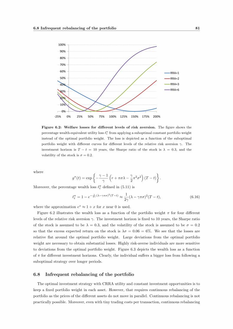
6.8 Infrequent rebalancing of the portfolio 81
40%
50%
60%
70%
80%
90%
100%
RRA=1
RRA=2
RRA=3
0%
10%
20%
30%
40%
50%
60%
70%
80%
90%
100%
-25% 0% 25% 50% 75% 100% 125% 150% 175% 200%
RRA=1
RRA=2
RRA=3
RRA=6
Figure 6.2: Welfare losses for different levels of risk aversion. The figure shows the
percentage wealth-equivalent utility loss `πt from applying a suboptimal constant portfolio weight
instead of the optimal portfolio weight. The loss is depicted as a function of the suboptimal
portfolio weight with different curves for different levels of the relative risk aversion γ. The
investment horizon is T − t = 10 years, the Sharpe ratio of the stock is λ = 0.3, and the
volatility of the stock is σ = 0.2.
where
gπ(t) = exp
−γ − 1
γ
(r + πσλ− γ
2π2σ2
)(T − t)
.
Moreover, the percentage wealth loss `πt defined in (5.11) is
`πt = 1− e−1
2γ (λ−γπσ)2(T−t) ≈ 1
2γ(λ− γπσ)2(T − t), (6.16)
where the approximation ex ≈ 1 + x for x near 0 is used.
Figure 6.2 illustrates the wealth loss as a function of the portfolio weight π for four different
levels of the relative risk aversion γ. The investment horizon is fixed to 10 years, the Sharpe ratio
of the stock is assumed to be λ = 0.3, and the volatility of the stock is assumed to be σ = 0.2
so that the excess expected return on the stock is λσ = 0.06 = 6%. We see that the losses are
relative flat around the optimal portfolio weight. Large deviations from the optimal portfolio
weight are necessary to obtain substantial losses. Highly risk-averse individuals are more sensitive
to deviations from the optimal portfolio weight. Figure 6.3 depicts the wealth loss as a function
of π for different investment horizons. Clearly, the individual suffers a bigger loss from following a
suboptimal strategy over longer periods.
6.8 Infrequent rebalancing of the portfolio
The optimal investment strategy with CRRA utility and constant investment opportunities is to
keep a fixed portfolio weight in each asset. However, that requires continuous rebalancing of the
portfolio as the prices of the different assets do not move in parallel. Continuous rebalancing is not
practically possible. Moreover, even with tiny trading costs per transaction, continuous rebalancing

82 Chapter 6. Asset allocation with constant investment opportunities
30%
40%
50%
60%
70%
80%
T=1
T=10
T=20
0%
10%
20%
30%
40%
50%
60%
70%
80%
-25% 0% 25% 50% 75% 100% 125% 150% 175% 200%
T=1
T=10
T=20
Figure 6.3: Welfare losses for different investment horizons. The figure shows the
percentage wealth-equivalent utility loss `πt from applying a suboptimal constant portfolio weight
instead of the optimal portfolio weight. The loss is depicted as a function of the suboptimal
portfolio weight with different curves for different investment horizons T − t. The relative risk
aversion is γ = 2, the Sharpe ratio of the stock is λ = 0.3, and the volatility of the stock is
σ = 0.2.
would be infinitely expensive. It is therefore interesting to see how bad it is to rebalance in a non-
continuous way. Let us disregard consumption in the following considerations and assume a single
risky asset.
A very simple strategy is to predetermine a finite number of trading dates. At each trading
date the portfolio is rebalanced so that the portfolio weights coincide with the solution for the
continuous time case. In between trading dates, the portfolio weights will deviate from the truly
optimal weights. Suppose that ∆t > 0 is the time period between any two adjacent trading dates.
Suppose the portfolio is rebalanced at time t so that the total wealth Wt is split into the amount
πWt invested in the stock and the amount (1−π)Wt in the riskfree asset. The gross return on the
stock until the next rebalancing is
St+∆t
St= exp
(r + σλ− 1
2σ2
)∆t+ σ(zt+∆t − zt)
,
and the gross return on the riskfree investment is expr∆t. The wealth at time t+∆t is therefore
Wt+∆t = πWt exp
(r + σλ− 1
2σ2
)∆t+ σ(zt+∆t − zt)
+ (1− π)Wt expr∆t
= Wter∆t
1 + π
[exp
(σλ− 1
2σ2
)∆t+ σ(zt+∆t − zt)
− 1
].
Seen at time t, the only random variable on the right-hand side is zt+∆t − zt ∼ N(0,∆t). The
discrete rebalancing strategy can be evaluated by Monte Carlo simulation.3 The wealth can be
simulated forward using the above relation by replacing zt+∆t − zt by εt+∆t
√∆t, where εt+∆t
3Monte Carlo simulation is described in most derivatives textbooks, e.g., Hull (2009) and Munk (2011).

6.8 Infrequent rebalancing of the portfolio 83
is a draw from the standard normal distribution, N(0, 1), with independent draws for different
time steps as the increments to the standard Brownian motion over non-overlapping intervals are
independent.4 We can generate a simulated value of the terminal wealth WT and compute the
utility u(WT ) = 11−γW
1−γT . By generating a large number, M , of samples Wm
T of terminal wealth,
we can take the average utility as an approximation of the expected utility of terminal wealth for
this discrete rebalancing strategy:
E[u(WT )] ≈ 1
M
M∑m=1
u (WmT ) .
We can then compare that (approximation of the) expected utility with the value function and
compute a percentage wealth-equivalent loss `t as defined in (5.11) and used above.
As an example, assume r = 0.02, σ = 0.2, and λ = 0.3, and consider an investor with a relative
risk aversion of γ = 2 and an investment horizon of T − t = 10 years. The optimal strategy
is to have π = 0.75 = 75% of the wealth invested in the stock at any point in time. If we fix
initial wealth to 1, the indirect utility will be −0.65377. In a Monte Carlo simulation procedure
implemented in Microsoft Excel, 2000 “antithetic” pairs of terminal wealth were simulated using
quarterly rebalancing.5 The average utility was−0.65547, which corresponds to a wealth-equivalent
loss of only 0.26% (in Exercise 6.5 you are asked to do similar experiments). This experiment
indicates that it is not important to rebalance the portfolio very frequently. Between two adjacent
rebalancing dates the portfolio weight of the stock can deviate somewhat from the optimal weight,
but the deviation is typically rather small, and we have already seen in the previous section that
expected utility is relatively insensitive to small deviations from the optimal strategy.
Rogers (2001) provides a more formal analysis of the impact of infrequent portfolio rebalancing.
Branger, Breuer, and Schlag (2010) perform a detailed Monte Carlo simulation study, also for some
models with stochastic investment opportunities that we will discuss in later chapters. Their study
4Some spread sheet applications, programming environments, and other software tools may have a built-in
procedure for generating such draws, but not all of them are of a good quality, i.e., if you use the procedure for
generating a number of such draws, the distribution of these draws may be quite different from the standard normal
distribution. Alternatively, you can generate draws from the N(0, 1) distribution by transforming draws from a
uniform distribution on the unit interval, a distribution we will denote by U [0, 1]. Most computer tools used for
financial applications have a built-in generator of random numbers from the U [0, 1] distribution, but there are also
algorithms for generating these draws that can easily be implemented in any programming environment, cf., e.g.,
Press, Teukolsky, Vetterling, and Flannery (2007, Ch. 7). A popular choice is the so-called Box-Muller transformation
suggested by Box and Muller (1958). Given two draws U1 and U2 from the uniform U [0, 1] distribution, ε1 and ε2
defined by
ε1 =√−2 lnU1 cos(2πU2), ε2 =
√−2 lnU1 sin(2πU2)
are two independent draws from the standard normal distribution. An alternative approach is to transform a draw
U from the U [0, 1] distribution into a draw ε from the N(0, 1) distribution by
ε = N−1(U),
where N−1(·) denotes the inverse of the probability distribution function N(·) associated with the standard normal
distribution, i.e., N(x) =∫ x−∞
1√2π
exp(−z2/2) dz. This follows from the fact that P(ε < a) = P(N−1(U) < a) =
P(U < N(a)) = N(a). Of course, this approach requires an implementation of the inverse normal distribution
N−1(·), which is not known in closed form. Again, some software tools (such as Microsoft Excel) have a built-in
algorithm for computing the inverse normal distribution, but the precision of the algorithm is generally unknown to
the user, and the computation is bound to be more time-consuming than when using the Box-Muller transformation.5The idea of antithetic variates is explained in most textbook presentations of Monte Carlo simulation, including
Hull (2009) and Munk (2011).

84 Chapter 6. Asset allocation with constant investment opportunities
confirms that for investment problems involving only stocks and bonds, relatively infrequent rebal-
ancing induces small wealth-equivalent losses. However, when derivatives are included, frequent
rebalancing is sometimes important.
6.9 Exercises
Exercise 6.1. Consider the optimal consumption and investment strategy for a CRRA investor
(with no labor income) in a market with constant r, µ, and σ, cf. Theorem 6.2. How does the
optimal strategy depend on time and the parameters of the model? (You may assume that only
one risky asset is traded.)
Exercise 6.2. Give a proof of Theorem 6.3.
Exercise 6.3. Verify the expressions (6.15) and (6.16). Try to create figures like Figures 6.2– 6.3.
Show that the alternative loss measure ˜t under the given assumptions becomes
˜t = e
12γ (λ−γπσ)2(T−t) − 1 ≈ 1
2γ(λ− γπσ)2(T − t),
so that the two loss measures are approximately the same for small deviations from the optimal
strategy.
Exercise 6.4. Assume a financial market with a constant risk-free rate r and risky assets with
constant µ and σ . Consider an investor with no income from non-financial sources and an indirect
utility function
J(W, t) = sup(cs,πs)s∈[t,T ]
EW,t
[∫ T
t
e−δ(s−t)u(cs) ds
],
where u now is a subsistence HARA function,
u(c) =(c− c)1−γ
1− γ
with c being the subsistence level of consumption. What is the optimal consumption and investment
strategy for this investor? Compare with the standard CRRA solution. Hint: How do you invest
to finance the subsistence level of consumption in the rest of your life? What is the cost of that
investment? The remaining wealth can be invested “freely”.
Exercise 6.5. Implement a Monte Carlo simulation to study the impact of infrequent trading
as explained in Section 6.8. Consider an investor with utility of terminal wealth only, a constant
relative risk aversion γ, and an investment horizon of T − t. The market consists of a riskfree asset
with a constant rate of return r and a single risky asset with volatility σ and a Sharpe ratio λ,
both assumed constant. Experiment with the frequency of trading, e.g., by considering 1, 4, 12,
and 52 trading dates per year. Compute wealth-equivalent losses for the discrete-trading strategies
compared to the continuous-time solution. How sensitive is the wealth-equivalent losses to the
parameters r, σ, λ, γ, and T − t?

CHAPTER 7
Stochastic investment opportunities: the general case
7.1 Introduction
In the previous chapter we analyzed the optimal investment/consumption decision under the
assumption of constant investment opportunities, i.e., constant interest rates, expected rates of
return, volatilities, and correlations. However, it is well-documented that some, if not all, of these
quantities vary over time in a stochastic manner. This situation is referred to as a stochastic
investment opportunity set. In this chapter we will study the dynamic investment/consumption
choice in a general financial market with stochastic investment opportunities. In later chapters we
will then focus on concrete models in which, for example, interest rates or expected excess stock
returns follow some specific dynamics.
The main effect of allowing investment opportunities to vary over time is easy to explain. Risk-
averse investors with time-additive utility are reluctant to substitute consumption over time, as
discussed in Section 2.7. To keep consumption stable across states and time, a (sufficiently) risk-
averse investor will therefore choose a portfolio with high positive returns in states with relatively
bad future investment opportunities (or bad future labor income) and conversely. This is what is
known as intertemporal hedging. The optimal investment strategy will thus be different from
the case with constant investment opportunities. From this argument, we also see that there will
be a close link between the optimal consumption strategy and the intertemporal hedging part of
the optimal investment strategy.
In the rest of this chapter we will formalize these issues in a general modeling framework. We will
continue to assume that the investor receives no non-financial income, i.e., no labor income, and
refer to Chapter 13 for the extension to the case with labor income. Throughout the chapter we
apply the dynamic programming approach, i.e., we focus on solving the Hamilton-Jacobi-Bellman
equation associated with the utility maximization problem.
85

86 Chapter 7. Stochastic investment opportunities: the general case
7.2 General utility functions
7.2.1 One-dimensional state variable
As in Section 5.3 we assume that there is a stochastically evolving state variable x = (xt) that
captures the variations in r, µ, and σ over time. The variations in the state variable x determine
the future expected returns and covariance structure in the financial market. For simplicity we will
first consider the case where x is one-dimensional and afterwards turn to the multi-dimensional
case.
The dynamics of the d risky asset prices is in this setting given by
dP t = diag(P t)[µ(xt, t) dt+ σ (xt, t) dzt
]= diag(P t)
[(r(xt)1 + σ (xt, t)λ(xt)
)dt+ σ (xt, t) dzt
].
We assume that x follows a one-dimensional diffusion process
dxt = m(xt) dt+ v(xt)> dzt + v(xt) dzt, (7.1)
where z is a one-dimensional standard Brownian motion independent of z. If v(xt) 6= 0, the market
is incomplete; otherwise, it is complete. Let
Σx(x) = v(x)>v(x) + v(x)2
denote the instantaneous variance of the state variable. For a given consumption strategy c = (ct)
and investment strategy π = (πt) the wealth evolves as
dWt = Wt
[r(xt) + π>
t σ (xt, t)λ(xt)]dt− ct dt+Wtπ
>t σ (xt, t) dzt,
and the indirect utility function is defined by
J(W,x, t) = sup(cs,πs)s∈[t,T ]
EW,x,t
[∫ T
t
e−δ(s−t)u(cs) ds+ e−δ(T−t)u(WT )
].
The HJB equation associated with this problem is
δJ(W,x, t) = LcJ(W,x, t) + LπJ(W,x, t) +∂J
∂t(W,x, t) + r(x)WJW (W,x, t)
+ Jx(W,x, t)m(x) +1
2Jxx(W,x, t)Σx(x),
(7.2)
with the terminal condition J(W,x, T ) = u(W ). Here
LcJ(W,x, t) = supc≥0u(c)− cJW (W,x, t) , (7.3)
LπJ(W,x, t) = supπ∈Rd
WJW (W,x, t)π>σ (x, t)λ(x) +
1
2JWW (W,x, t)W 2π>σ (x, t)σ (x, t)>π
+ JWx(W,x, t)Wπ>σ (x, t)v(x).
(7.4)
The first-order condition with respect to c is
u′(c) = JW (W,x, t)
so that the (candidate) optimal consumption strategy is
c∗t = C(W ∗t , xt, t),

7.2 General utility functions 87
where
C(W,x, t) = Iu(JW (W,x, t)) (7.5)
and, as before, Iu(·) is the inverse of u′(·). Substituting the maximizing c back into (7.3), we get
LcJ(W,x, t) = u (Iu(JW (W,x, t)))− Iu(JW (W,x, t))JW (W,x, t). (7.6)
Note that these relations are exactly as in the case with constant investment opportunities studied
in Section 6.2 with the only exception that the indirect utility function now depends on the state
variable x.
The first-order condition with respect to π is different than with constant investment opportu-
nities:
JW (W,x, t)Wσ (x, t)λ(x) + JWW (W,x, t)W 2σ (x, t)σ (x, t)>π + JWx(W,x, t)Wσ (x, t)v(x) = 0
so that the candidate optimal portfolio is
π∗t = Π(W ∗t , xt, t),
where
Π(W,x, t) = − JW (W,x, t)
WJWW (W,x, t)
(σ (x, t)>
)−1λ(x)− JWx(W,x, t)
WJWW (W,x, t)
(σ (x, t)>
)−1v(x). (7.7)
Substituting the maximizing π back into (7.4) and simplifying, we get
LπJ(W,x, t) = −1
2‖λ(x)‖2 JW (W,x, t)2
JWW (W,x, t)− 1
2‖v(x)‖2 JWx(W,x, t)2
JWW (W,x, t)
− v(x)>λ(x)JW (W,x, t)JWx(W,x, t)
JWW (W,x, t).
(7.8)
Let us take a closer look at the portfolio (7.7). As the horizon shrinks, the indirect utility
function J(W,x, t) approaches the terminal utility function u(W ) which is independent of the
state x. Consequently, the derivative JWx(W,x, t) and hence the last term of the portfolio will
approach zero as t → T . In other words, very short-term investors do not hedge. The last term
will also disappear for “non-instantaneous” investors in two special cases:
(1) JWx(W,x, t) ≡ 0: The state variable does not affect the marginal utility of the investor. As
we shall see below this is always true for investors with logarithmic utility. Such an investor
is not interested in hedging changes in the state variable.
(2) v(x) ≡ 0: The state variable is uncorrelated with instantaneous returns on the traded assets.
In this case the investor is not able to hedge changes in the state variable.
In all other cases the state variable induces an additional term to the optimal portfolio relative to
the case of constant investment opportunities. From (7.7) we have the following important result:
Theorem 7.1 (Three-fund separation). All investors will combine (1) the locally risk-free asset
(“the bank account”), (2) the tangency portfolio given by the weights
πtant =
1
1>(σ (xt, t)>
)−1λ(xt)
(σ (xt, t)
>)−1
λ(xt),
and (3) the hedge portfolio given by the weights
πhdgt =
1
1>(σ (xt, t)>
)−1v(xt)
(σ (xt, t)
>)−1
v(xt).

88 Chapter 7. Stochastic investment opportunities: the general case
Note that the composition of the two risky funds varies over time due to fluctuations in the state
variable. It is no longer true that all investors will hold different risky assets in the same proportion,
i.e., the fractions πi/πj will be investor-specific since different investors may put different weights on
the two portfolios of risky assets. The tangency portfolio has the same interpretation as previously.
The position in the portfolio πhdg is the change in the optimal investment strategy due to the
stochastic variations in the investment opportunity set, hence the name “hedge portfolio”. The next
theorem shows that among all portfolios the hedge portfolio has the maximal absolute correlation
with the state variable. In that sense it is the portfolio that is best at hedging changes in the state
variable. In a complete market the maximal correlation is one and the hedge portfolio basically
replicates the dynamics of the state variable.
Theorem 7.2. The absolute value of the instantaneous correlation between the change in the value
of an investment strategy and the change in the state variable is maximized for the investment
strategy πt = πhdgt .
Proof. The value process of an investment strategy π = (πt) has dynamics
dV πt = V πt(r(xt) + π>
t σ (xt, t)λ(xt))dt+ V πt π
>t σ (xt, t) dzt.
The instantaneous variance rate is (V πt )2π>t σ (xt, t)σ (xt, t)
>πt and the instantaneous covariance
rate with the state variable is V πt π>t σ (xt, t)v(xt). Hence, the square of the instantaneous correla-
tion is
ρ2 ≡(V πt π
>t σ (xt, t)v(xt)
)2((V πt )2π>
t σ (xt, t)σ (xt, t)>πt)
Σx(xt)
=(π>t σ(xt, t)v(xt))
2(π>t σ (xt, t)σ (xt, t)>πt
)Σx(xt)
.
The portfolio that maximizes ρ2 will also maximize the absolute correlation |ρ|. The first-order
condition for the maximization implies that
σ (xt, t)v(xt)(π>t σ (xt, t)σ (xt, t)
>πt)
=(π>t σ (xt, t)v(xt)
)σ (xt, t)σ (xt, t)
>πt.
Multiplying through by the inverse of σ (xt, t)σ (xt, t)>, we arrive at(
σ (xt, t)>)−1
v(xt)(π>t σ (xt, t)σ (xt, t)
>πt)
=(π>t σ (xt, t)v(xt)
)πt,
which we want to solve for πt. The sum of the elements of the vector on the left-hand side is
1>(σ (xt, t)
>)−1
v(xt)(π>t σ (xt, t)σ (xt, t)
>πt), while the sum of the elements of the right-hand
side vector is π>t σ (xt, t)v(xt) since 1>πt = 1. Dividing each side by the sum of the elements, we
obtain (σ (xt, t)
>)−1
v(xt)
1>(σ (xt, t)>
)−1v(xt)
= πt,
as was to be shown.
Let us focus for a moment on the case with a single risky asset so that both σ(x, t) and v(x)
are scalars. The hedge term in π∗t can then be written as − JWx
WJWW
vσ . Note that JWW < 0 by
concavity. If v and σ have the same sign, then the return of the risky asset will be positively

7.2 General utility functions 89
correlated with changes in the state variable. In this case we see that the hedge demand on the
asset is positive if marginal utility JW is increasing in x so that JWx > 0. This makes good sense:
relative to the situation with a constant investment opportunity set, the agent will devote a larger
fraction of wealth to a risky asset that has a high return in states of the world where marginal
utility is high. Conversely, if v and σ have opposite signs so that they are negatively correlated.
Here is another interpretation of the optimal portfolio strategy, following Ingersoll (1987, p. 282):
Theorem 7.3. The optimal portfolio strategy π∗ is the one that minimizes fluctuations in con-
sumption over time among all portfolio strategies with the same expected rate of return as π∗.
Proof. The expected rate of return on the optimal portfolio in (7.7) is
µ∗(x, t) = r(x) + (π∗t )>(µ(x, t)− r(x)1).
The consumption rate is given by
c∗t = C(Wt, xt, t).
An application of Ito’s Lemma yield
dc∗t = . . . dt+(CW (Wt, xt, t)Wtπ
>t σ (xt, t)
+ Cx(Wt, xt, t)v(xt)>)dzt + Cx(Wt, xt, t)v(xt) dzt,
where we leave the drift term unspecified and the subscripts on C denote partial derivatives. It
follows that the instantaneous variance rate of consumption is equal to
σ2c ≡ CW (W,x, t)2W 2π>σ (x, t)σ (x, t)>π + Cx(W,x, t)2Σx(x)
+ 2CW (W,x, t)Cx(W,x, t)Wπ>σ (x, t)v(x).
Now consider the problem of minimizing σ2c over all portfolios π that have an expected rate of
return equal to µ∗(x, t), i.e., portfolios π with r(x) + π>σ (x, t)λ(x) = µ∗(x, t). Forming the
Lagrangian
L = σ2c + ψ
[µ∗(x, t)− r(x)− π>σ (x, t)λ(x)
]we find the optimality condition
π∗∗ =ψ
2CW (W,x, t)2W 2
(σ (x, t)>
)−1λ(x)− Cx(W,x, t)
WCW (W,x, t)
(σ (x, t)>
)−1v(x).
Differentiating the envelope condition u′(C(W,x, t)) = JW (W,x, t) along the optimal consumption
path with respect to W we get
u′′(C(W,x, t))CW (W,x, t) = JWW (W,x, t)
and by differentiating with respect to x we get
u′′(C(W,x, t))Cx(W,x, t) = JWx(W,x, t).
Hence,Cx(W,x, t)
WCW (W,x, t)=
JWx(W,x, t)
WJWW (W,x, t)
so that the second terms in π∗ and π∗∗ are identical. The first term in π∗∗ is proportional to the
first term in π∗ and since π∗∗ is chosen such that it has the same expected rate of return as π∗,
the first terms must also coincide. In total, π∗∗ = π∗, which was to be shown.

90 Chapter 7. Stochastic investment opportunities: the general case
On the other hand, if we minimize the instantaneous variance rate of wealth, i.e., σ2W =
π>σ (x, t)σ (x, t)>π, over all portfolios π having the same expected rate of return as π∗, we get
π∗∗ = ψ(σ (x, t)>
)−1λ(x).
This only involves the tangency portfolio. We can conclude that the investor is concerned about
fluctuations over time in consumption, not in wealth.
Above, we discussed the general expressions for the optimal consumption and investment strategy
in the presence of a state variable. But these were expressed in terms of the unknown indirect
utility function. How do we proceed to find concrete solutions?
Substituting (7.6) and (7.8) back into the HJB equation (7.2) and gathering terms, we get the
second order PDE
δJ(W,x, t) = u (Iu(JW (W,x, t)))− JW (W,x, t)Iu(JW (W,x, t)) +∂J
∂t(W,x, t) + r(x)WJW (W,x, t)
− 1
2
JW (W,x, t)2
JWW (W,x, t)‖λ(x)‖2 + Jx(W,x, t)m(x) +
1
2Jxx(W,x, t)Σx(x)
− 1
2
JWx(W,x, t)2
JWW (W,x, t)‖v(x)‖2 − JW (W,x, t)JWx(W,x, t)
JWW (W,x, t)λ(x)>v(x).
(7.9)
If this PDE has a solution J(W,x, t) satisfying the terminal condition J(W,x, T ) = u(W ) and the
strategy defined by (7.5) and (7.7) is feasible (satisfies the technical conditions), then we know
from the verification theorem that this strategy is indeed the optimal consumption and investment
strategy and the function J(W,x, t) is indeed the indirect utility function. With no utility from
intermediate consumption, i.e., u ≡ 0, the first two terms of the right-hand side of (7.9) vanish.
Although the PDE (7.9) looks very complicated, closed-form solutions can be found for a number
of interesting model specifications as we shall see later in this chapter and in other chapters.
7.2.2 Multi-dimensional state variable
Suppose now that the state variable x is k-dimensional and follows the diffusion process
dxt = m(xt) dt+ v(xt)> dzt + v(xt) dzt,
where m now is a k-vector valued function, v is a (d × k)-matrix valued function, v is a (k × k)-
matrix valued function, and z is a k-dimensional standard Brownian motion independent of z.
The instantaneous variance-covariance matrix of the state variable is the (k × k) matrix
Σx(x) = v(x)>v(x) + v(x)v(x)>.
denote the instantaneous variance of the state variable. As explained in Section 5.3, the HJB
equation is then
δJ(W,x, t) = LcJ(W,x, t) + LπJ(W,x, t) +∂J
∂t(W,x, t) + r(x)WJW (W,x, t)
+ Jx(W,x, t)>m(x) +1
2tr(Jxx(W,x, t)Σx(x)
),

7.2 General utility functions 91
where
LcJ(W,x, t) = supc≥0u(c)− cJW (W,x, t) ,
LπJ(W,x, t) = supπ∈Rd
WJW (W,x, t)π>σ (x, t)λ(x) +
1
2JWW (W,x, t)W 2π>σ (x, t)σ (x, t)>π
+Wπ>σ (x, t)v(x)JWx(W,x, t).
Analogously to the case with a one-dimensional state variable discussed in the previous section,
the (candidate) optimal consumption strategy is
c∗t = C(W ∗t ,xt, t),
where
C(W,x, t) = Iu(JW (W,x, t)),
so that
LcJ(W,x, t) = u (Iu(JW (W,x, t)))− Iu(JW (W,x, t))JW (W,x, t).
Likewise, the candidate optimal portfolio is
π∗t = Π(W ∗t ,xt, t),
where
Π(W,x, t) = − JW (W,x, t)
WJWW (W,x, t)
(σ (x, t)>
)−1λ(x)−
(σ (x, t)>
)−1v(x)
JWx(W,x, t)
WJWW (W,x, t), (7.10)
and
LπJ(W,x, t) = −1
2
JW (W,x, t)2
JWW (W,x, t)‖λ(x)‖2 − λ(x)>v(x)
JW (W,x, t)JWx(W,x, t)
JWW (W,x, t)
− 1
2JWW (W,x, t)JWx(W,x, t)>v(x)>v(x)JWx(W,x, t).
We can split up the last term of the optimal portfolio into k terms, one for each element of the
state variable:
Π(W,x, t) = − JW (W,x, t)
WJWW (W,x, t)
(σ (x, t)>
)−1λ(x)−
k∑j=1
(σ (x, t)>
)−1
v1j(x)
v2j(x)...
vdj(x)
JWxj (W,x, t)
WJWW (W,x, t).
Each of the terms in the sum has the interpretation as a fund hedging changes in one element of
the state variable. Therefore, we have (k + 2)-fund separation: all investors are satisfied with
access to trade in the risk-free asset, the tangency portfolio, and k hedge funds.
Substituting LcJ and LπJ back into the HJB equation and gathering terms, we get the second-
order PDE
δJ(W,x, t) = u (Iu(JW (W,x, t)))− JW (W,x, t)Iu(JW (W,x, t)) +∂J
∂t(W,x, t)
+ r(x)WJW (W,x, t)− 1
2
JW (W,x, t)2
JWW (W,x, t)‖λ(x)‖2 + Jx(W,x, t)>m(x)
+1
2tr(Jxx(W,x, t)Σx(x)
)− λ(x)>v(x)
JW (W,x, t)JWx(W,x, t)
JWW (W,x, t)
− 1
2JWW (W,x, t)JWx(W,x, t)>v(x)>v(x)JWx(W,x, t).
(7.11)

92 Chapter 7. Stochastic investment opportunities: the general case
As before, the first two terms on the right-hand side are not present when the agent has no utility
from intermediate consumption.
7.2.3 What risks are to be hedged?
It may appear from the analysis above that investors would want to hedge all variables affecting
rt, µt, and σ t, but this is actually not so. We will show that the only risks the agent will want to
hedge are those affecting rt and λt.
Since σ t and thus σ>t are assumed to be non-singular, we can think of the investor choosing the
“volatility vector of wealth” ϕt = σ>t πt directly rather than πt. In these terms wealth evolves as
dWt = Wt [rt +ϕ>t λt] dt− ct dt+Wtϕ
>t dzt.
The indirect utility function is
Jt = sup(c,ϕ)
Et
[∫ T
t
e−δ(s−t)u(cs) ds+ e−δ(T−t)u(WT )
].
Note that this optimization problem does not involve µt or σ t. Assuming now that there is a
variable xt so that
rt = r(xt), λt = λ(xt),
then Jt = J(Wt,xt, t) and we can use the dynamic programming approach.
For a multidimensional x we will get the optimal wealth volatility vector
ϕt = − JW (Wt,xt, t)
WtJWW (Wt,xt, t)λ(xt)− v(xt)
JWx(Wt,xt, t)
WtJWW (Wt,xt, t).
Hence, the optimal portfolio strategy is
πt = − JW (Wt,xt, t)
WtJWW (Wt,xt, t)
(σ>t
)−1λ(xt)−
(σ>t
)−1v(xt)
JWx(Wt,xt, t)
WtJWW (Wt,xt, t).
We can conclude from this analysis that the investor will only hedge the variables that affect the
short-term interest rate and the market prices of risk (this is of course only true within the present
framework; e.g., an investor with stochastic income will also want to hedge the income risk).
Stochastic variations in µt and σ t are only interesting to the extent that they cause stochastic
variations in the market price of risk! One could imagine a market where volatilities vary stochas-
tically but expected rates of return follow the variations in volatilities so that the market price of
risk is constant over time. In such a market no agent would hedge the variations in volatilities and
expected rates of return. Similar observations were made by Detemple, Garcia, and Rindisbacher
(2003) and Munk and Sørensen (2004). The volatility matrix σ t of the risky assets becomes rel-
evant when the agent wants to find a portfolio πt that will generate the desired wealth volatility
vector ϕt.
In fact, the statement above can be strengthened slightly. Look at the PDE (7.11). Suppose
that both r and ‖λ‖2 are independent of x. Then the function J(W, t) that satisfies the simple
PDE
δJ(W, t) = u (Iu(JW (W, t)))− JW (W, t)Iu(JW (W, t)) +∂J
∂t(W, t)
+ rWJW (W, t)− 1
2
JW (W, t)2
JWW (W, t)‖λ‖2

7.3 CRRA utility 93
with J(W,T ) = u(W ) will also solve the full HJB equation (7.9) as all derivatives with respect to x
will be zero. Consequently, the hedge term in (7.10) disappears. In other words, the investor will
only hedge stochastic variations that affect the short-term interest rate rt and the squared market
prices of risk1
‖λt‖2 = (µt − rt1)> (σ tσ
>t
)−1(µt − rt1) .
Nielsen and Vassalou (2006) show that this result is also true for non-Markov dynamics of prices.
We summarize this in the following theorem:
Theorem 7.4. Investors with time-additive utility functions and no income from non-financial
sources will only hedge stochastic variations in the short-term interest rate rt and in the squared
market prices of risk ‖λt‖2.
There is a very intuitive interpretation of this result, which we can see after a few computations:
The tangency portfolio is in general given by [see (6.8)]
πtant =
1
1>(σ>t
)−1λt
(σ>t
)−1λt.
The expected excess rate of return on the tangency portfolio is(πtant
)>(µt − rt1) =
1
1>(σ>t
)−1λt‖λt‖2.
The volatility (instantaneous standard deviation) of the tangency portfolio is√(πtan
t )>σ tσ>
t πtant =
1
1>(σ>t
)−1λt‖λt‖.
The slope of the instantaneous capital market line is therefore equal to ‖λt‖. (In a setting with a
single risky asset, λt = (µt − rt)/σt and ‖λt‖ = λt.) In a static framework the optimal portfolio is
determined by the position of the capital market line, i.e., (1) the intercept which is equal to the
risk-free rate of return and (2) the slope which is the Sharpe ratio of the tangency portfolio. It is
therefore natural that investors in a dynamic framework only are concerned about the variations
in these two variables.
7.3 CRRA utility
In this section we assume that the investor has time-additive expected CRRA utility with a
constant relative risk aversion γ > 1. The case γ = 1 that corresponds to logarithmic utility has
to be analyzed separately (see Section 7.4). However, it turns out that when γ is put equal to 1 in
the optimal strategies derived for γ > 1 we obtain the optimal strategies derived for logarithmic
utility.
7.3.1 One-dimensional state variable
Consider the indirect utility function with CRRA utility:
J(W,x, t) = sup(cs,πs)s∈[t,T ]
EW,x,t
[ε1
∫ T
t
e−δ(s−t)c1−γs
1− γds+ ε2e
−δ(T−t)W1−γT
1− γ
],
1Examples where ‖λ‖2 is constant, but λ itself is not, can be given [see Nielsen and Vassalou (2006)], but seem
rather contrived.

94 Chapter 7. Stochastic investment opportunities: the general case
where ε1 and ε2 are greater than or equal to zero with at least one of them being non-zero. We
set up a conjecture for the form of J using the same arguments as we did in the case of constant
investment opportunities. Due to the linearity of the wealth dynamics it seems reasonable to guess
that if the strategy (c∗,π∗) is optimal with time t wealth W and state x and the corresponding
wealth process W ∗, then the strategy (kc∗,π∗) will be optimal with time t wealth kW and state
x and the corresponding wealth process kW ∗. If this is true, then
J(kW, x, t) = Et
[ε1
∫ T
t
e−δ(s−t)(kc∗s)
1−γ
1− γds+ ε2e
−δ(T−t) (kW ∗T )1−γ
1− γ
]
= k1−γ Et
[ε1
∫ T
t
e−δ(s−t)(c∗s)
1−γ
1− γds+ ε2e
−δ(T−t) (W ∗T )1−γ
1− γ
]= k1−γJ(W,x, t),
i.e., the indirect utility function is homogeneous of degree 1 − γ in the wealth level. Inserting
k = 1/W and rearranging, we get
J(W,x, t) =1
1− γg(x, t)γW 1−γ ,
where g(x, t)γ = (1− γ)J(1, x, t). From the terminal condition J(W,x, T ) = ε2W1−γ/(1− γ), we
have that g(x, T )γ = ε2.
The relevant derivatives of J are
JW (W,x, t) = g(x, t)γW−γ ,
JWW (W,x, t) = −γg(x, t)γW−γ−1,
Jx(W,x, t) =γ
1− γg(x, t)γ−1gx(x, t)W 1−γ ,
Jxx(W,x, t) = −γg(x, t)γ−2gx(x, t)2W 1−γ +γ
1− γg(x, t)γ−1gxx(x, t)W 1−γ ,
JWx(W,x, t) = γg(x, t)γ−1gx(x, t)W−γ ,
∂J
∂t(W,x, t) =
γ
1− γg(x, t)γ−1 ∂g
∂t(x, t)W 1−γ .
Substituting into (7.7), the optimal investment strategy becomes
Π(W,x, t) =1
γ
(σ (x, t)>
)−1λ(x) +
gx(x, t)
g(x, t)
(σ (x, t)>
)−1v(x), (7.12)
and from (7.5) the optimal consumption strategy becomes
C(W,x, t) = ε1/γ1
W
g(x, t),
which, of course, is zero if the investor obtains no utility from intermediate consumption. It is
optimal to consume a time- and state-dependent fraction of wealth. The optimal fractions of
wealth allocated to the various risky assets are independent of the level of wealth, but depend on
the state and time.
Note again the close link between the optimal consumption strategy and the intertemporal
hedging term in the optimal investment strategy. With intermediate consumption the function
g(x, t) is the optimal wealth-to-consumption ratio. By Ito’s Lemma, the dynamics will be
dg(xt, t) = g(xt, t)
[. . . dt+
gx(x, t)
g(x, t)v(xt)
> dzt +gx(x, t)
g(x, t)v(xt) dzt
].

7.3 CRRA utility 95
The dynamics of the value of a given portfolio π is
dV πt = V πt[(r(xt) + π>
t σ (xt, t)λ(xt))dt+ π>
t σ (xt, t) dzt].
We see that the hedge portfolio is matching the sensitivity of the optimal wealth-to-consumption
ratio with respect to the hedgeable shocks represented by dzt.
Inserting the derivatives above into (7.9) and simplifying, we get that g(x, t) must solve the PDE
0 = ε1/γ1 −
(δ
γ+γ − 1
γr(x) +
γ − 1
2γ2‖λ(x)‖2
)g(x, t) +
(m(x)− γ − 1
γλ(x)>v(x)
)gx(x, t)
+∂g
∂t(x, t) +
1
2gxx(x, t)Σx(x) +
γ − 1
2v(x)2 gx(x, t)2
g(x, t)
(7.13)
with the terminal condition g(x, T ) = ε1/γ2 . In the case with no intermediate consumption we have
ε1 = 0, and we can without loss of generality assume ε2 = 1 and δ = 0. If we write
g(x, t) ≡ g(x, t;T ) = exp
−γ − 1
γH(x, T − t)
,
then H(x, τ) has to solve the simpler PDE
0 =r(x) +1
2γ‖λ(x)‖2 − ∂H
∂τ(x, τ) +
(m(x)− γ − 1
γλ(x)>v(x)
)Hx(x, τ)
+1
2Σx(x)Hxx(x, τ)− γ − 1
2γ
(Σx(x) + (γ − 1)v(x)2
)Hx(x, τ)2
(7.14)
with the condition H(x, 0) = 0.
Theorem 7.5. With CRRA utility of terminal wealth only (ε1 = 0, ε2 = 1, δ = 0), the indirect
utility function is
J(W,x, t) =1
1− γe−(γ−1)H(x,T−t)W 1−γ =
1
1− γ
(WeH(x,T−t)
)1−γ,
and the optimal investment strategy in (7.12) can be rewritten as
Π(W,x, t) =1
γ
(σ (x, t)>
)−1λ(x)− γ − 1
γHx(x, T − t)
(σ (x, t)>
)−1v(x),
where H(x, τ) solves the PDE (7.14) with initial condition H(x, 0) = 0.
When the market is complete so that v(x) ≡ 0, the next theorem shows that the solution to
the utility maximization problem with intermediate consumption follows from the solution to the
problem of maximizing utility of wealth at a single point in time. The proof is left for Exercise 7.1.
Theorem 7.6. Let H(x, τ) be the solution to the PDE
0 =r(x) +1
2γ‖λ(x)‖2 − ∂H
∂τ(x, τ) +
(m(x)− γ − 1
γλ(x)>v(x)
)Hx(x, τ)
+1
2Σx(x)Hxx(x, τ)− γ − 1
2γΣx(x)Hx(x, τ)2
(7.15)
with terminal condition H(x, 0) = 0. Define
g(x, t; s) = exp
− δγ
(s− t)− γ − 1
γH(x, s− t)
.

96 Chapter 7. Stochastic investment opportunities: the general case
Then the solution to the PDE (7.13) with v(x) ≡ 0 is
g(x, t) = ε1γ
1
∫ T
t
g(x, t; s) ds+ ε1γ
2 g(x, t;T ).
In a complete market (v(x) ≡ 0), the maximization of CRRA utility of intermediate consumption
and/or terminal wealth leads to the indirect utility J(W,x, t) = 11−γ g(x, t)γW 1−γ , the optimal
consumption strategy is
C(W,x, t) = ε1/γ1
W
g(x, t)=
(∫ T
t
g(x, t; s) ds+
(ε2
ε1
) 1γ
g(x, t;T )
)−1
W,
and the optimal investment strategy is
Π(W,x, t) =1
γ
(σ (x, t)>
)−1λ(x)− γ − 1
γD(x, t, T )
(σ (x, t)>
)−1v(x),
where
D(x, t, T ) =
∫ TtHx(x, s− t)g(x, t; s) ds+ (ε2/ε1)
1γ Hx(x, T − t)g(x, t;T )∫ T
tg(x, t; s) ds+ (ε2/ε1)
1γ g(x, t;T )
.
The solution for the case with utility of intermediate consumption is thus obtained by simply
integrating up the solution for the case with utility of wealth at each of the fixed time horizons
over the remaining life-time [t, T ]. In any specific case with complete markets, the key challenge is
therefore to solve the PDE (7.15).
The PDE (7.14)—and thus the special case (7.15)—has a nice solution in a large class of in-
teresting models as we will show below. This leads to closed-form solutions to the power utility
maximization problem with terminal wealth only and—if the market is complete—with interme-
diate consumption. If the market is incomplete, the power utility maximization problem with
intermediate consumption is generally intractable, but the PDE (7.13) can be solved numerically.
7.3.2 Affine models
In this and the following subsection we will look at models in which the optimal portfolio and
consumption strategies of a CRRA investor can be derived in closed-form. In some of these cases
we can obtain explicit solutions, in other cases the solution involves time-dependent functions
that can be found by numerically solving ordinary differential equations. Many of our concrete
examples in the following chapters are special cases of these models. In this section we will discuss
so-called affine models, while the next section focuses on the so-called quadratic models. The
results presented are similar to those obtained by Liu (1999, 2007). For notational simplicity we
shall assume that the state variable is one-dimensional with dynamics given by (7.1). We will
briefly discuss solutions to problems with a multi-dimensional state variable in Section 7.3.4.
As explained above, the key is to solve the PDE (7.14) for H(x, τ) with the initial condition
H(x, 0) = 0. Let us consider when we can find a solution of the affine form
H(x, τ) = A0(τ) +A1(τ)x,
where A0 and A1 are real-valued deterministic functions that have to satisfy A0(0) = A1(0) = 0

7.3 CRRA utility 97
to meet the initial condition. Substituting into (7.14), we find
0 = r(x) +1
2γ‖λ(x)‖2 −A′0(τ)−A′1(τ)x+
(m(x)− γ − 1
γλ(x)>v(x)
)A1(τ)
− γ − 1
2γ
(Σx(x) + (γ − 1)v(x)2
)A1(τ)2.
(7.16)
If r(x), ‖λ(x)‖2, m(x), v(x)>λ(x), ‖v(x)‖2, and v(x)2 are all affine functions2 of x, then we can
find two ordinary differential equations for A0 and A1. In order to see this, suppose that
r(x) = r0 + r1x, (7.17)
m(x) = m0 +m1x, (7.18)
v(x) =√v0 + v1x
for some constants r0, r1,m0,m1, v0, and v1. Of course, we should have that v0 + v1x ≥ 0 for all
possible values of x, which is easily satisfied if either v0 or v1 are zero and the other parameter is pos-
itive. The term ‖λ(x)‖2 will be affine in x if each element of the vector λ(x) = (λ1(x), . . . , λd(x))>
is of the form λi(x) =√λi0 + λi1x since then
‖λ(x)‖2 =
d∑i=1
λi(x)2 =
d∑i=1
(λi0 + λi1x) =
(d∑i=1
λi0
)+
(d∑i=1
λi1
)x ≡ Λ0 + Λ1x. (7.19)
Similarly, the term ‖v(x)‖2 will be affine in x if each element of the vector v(x) = (v1(x), . . . , vd(x))>
is of the form vi(x) =√vi0 + vi1x. Then we have
‖v(x)‖2 =
d∑i=1
vi(x)2 =
d∑i=1
(vi0 + vi1x) =
(d∑i=1
vi0
)+
(d∑i=1
vi1
)x ≡ V0 + V1x. (7.20)
In addition, we must have that v(x)>λ(x) is affine in x. With the specifications of λ(x) and v(x)
just given, we have
v(x)>λ(x) =
d∑i=1
vi(x)λi(x) =
d∑i=1
√(vi0 + vi1x)(λi0 + λi1x).
This will only be affine in x if, for each i, we have either
(i) vi0 = λi0 = 0, or
(ii) vi1 = λi1 = 0, or
(iii) vi0 = λi0 and vi1 = λi1.
To encompass all possible situations let us write
v(x)>λ(x) = K0 +K1x, (7.21)
where K0 and K1 are real-valued parameters. If we substitute (7.17)–(7.21) into (7.16) and use
the fact that (7.16) must hold for all values of x and all τ , we obtain a system of two ordinary
2A real-valued function is said to be an affine function of the k-vector x, if it can be written as a1 +a>2 x, where
a1 is a constant scalar and a2 is a constant k-vector (possibly zero so that a constant is also included in the set of
affine functions). A vector- or matrix-valued function is said to be affine if all its elements are affine.

98 Chapter 7. Stochastic investment opportunities: the general case
differential equations for A0 and A1:
A′0(τ) = r0 +Λ0
2γ+
(m0 −
γ − 1
γK0
)A1(τ)− γ − 1
2γ(V0 + γv0)A1(τ)2,
A′1(τ) = r1 +Λ1
2γ+
(m1 −
γ − 1
γK1
)A1(τ)− γ − 1
2γ(V1 + γv1)A1(τ)2. (7.22)
These equations are to be solved with the initial conditions A0(0) = A1(0) = 0.
First (7.22) is solved for A1(τ). From Theorem C.2, we can make the following conclusion.
Suppose that (m1 −
γ − 1
γK1
)2
+ 2γ − 1
γ
(r1 +
Λ1
2γ
)(V1 + γv1) > 0 (7.23)
and define
ν =
√(m1 −
γ − 1
γK1
)2
+ 2γ − 1
γ
(r1 +
Λ1
2γ
)(V1 + γv1).
Then the solution to (7.22) with A1(0) = 0 is
A1(τ) =2(r1 + Λ1
2γ
)(eντ − 1)(
ν + γ−1γ K1 −m1
)(eντ − 1) + 2ν
. (7.24)
Since A0(τ) = A0(τ)−A0(0) =∫ τ
0A′0(s) ds, we can afterwards compute A0(τ) as
A0(τ) =
(r0 +
Λ0
2γ
)τ +
(m0 −
γ − 1
γK0
)∫ τ
0
A1(s) ds− γ − 1
2γ(V0 + γv0)
∫ τ
0
A1(s)2 ds. (7.25)
Also from Theorem C.2, we have that∫ τ
0
A1(s) ds = − 2γ
(γ − 1) (V1 + γv1)
1
2
(ν +
γ − 1
γK1 −m1
)τ + ln
2ν(ν + γ−1
γ K1 −m1
)(eντ − 1) + 2ν
and ∫ τ
0
A1(s)2 ds = - ugly expression to be filled in -
Combining these findings with Theorem 7.5, we arrive at the following conclusion:3
Theorem 7.7. Assume that r(x), ‖λ(x)‖2, m(x), v(x)>λ(x), ‖v(x)‖2, and v(x)2 are all affine
functions of x and given by (7.17)–(7.21), and that the parameter condition (7.23) holds. For an
investor with CRRA utility from terminal wealth only, the indirect utility function is then given by
J(W,x, t) =1
1− γ
(WeA0(T−t)+A1(T−t)x
)1−γ,
where A1 is given by (7.24) and A0 is given by (7.25). The optimal investment strategy is given by
Π(W,x, t) =1
γ
(σ (x, t)>
)−1λ(x)− γ − 1
γ
(σ (x, t)>
)−1v(x)A1(T − t).
In some important special cases, A0 and A1 simplify considerably. For example, if V1 + γv1 = 0
so that the second-order term in (7.22) vanishes then (again see Theorem C.2)
ν = −(m1 −
γ − 1
γK1
)=γ − 1
γK1 −m1,
3Note the close connection between the analysis above and the analysis for so-called affine models of the term
structure of interest rates, see e.g., Duffie and Kan (1996), Dai and Singleton (2000), or Munk (2011).

7.3 CRRA utility 99
so that A1(τ) reduces to
A1(τ) =r1 + Λ1
2γ
ν
(1− e−ντ
).
In this case the integrals in (7.25) are also relatively simple:∫ τ
0
A1(u) du =1
m1 − γ−1γ K1
((r1 +
Λ1
2γ
)τ −A1(τ)
),
∫ τ
0
A1(u)2 du =1(
r1 + Λ1
2γ
)(m1 − γ−1
γ K1
)(r1 + Λ1
2γ
)3
τ −A1(τ)
m1 − γ−1γ K1
− A1(τ)2
2(r1 + Λ1
2γ
) .
This special case is relevant in Chapter 10.
For the problem with utility of intermediate consumption, we can provide a solution for the
complete markets case (v(x) ≡ 0) by combining the above computations with Theorem 7.6. The
only difference in the relevant ODEs, and thus in their solutions, is that we have to impose the
restriction v0 = v1 = 0 because of the complete market assumption.
Theorem 7.8. Assume a complete financial market (v(x) ≡ 0) in which r(x), ‖λ(x)‖2, m(x),
v(x)>λ(x), and ‖v(x)‖2 are all affine functions of x and given by (7.17), (7.18), (7.19), (7.20),
and (7.21). Imposing the restriction v0 = v1 = 0, assume that the parameter condition (7.23) holds,
and let A1 and A0 be given by (7.24) and (7.25). Define
g(x, t; s) = exp
− δγ
(s− t)− γ − 1
γ(A0(s− t) +A1(s− t)x)
.
For an investor with CRRA utility from intermediate consumption and possibly terminal wealth,
the indirect utility function is then given by
J(W,x, t) =1
1− γ
(ε
1γ
1
∫ T
t
g(x, t; s) ds+ ε1γ
2 g(x, t;T )
)γW 1−γ ,
the optimal consumption strategy is
C(W,x, t) =
(∫ T
t
g(x, t; s) ds+
(ε2
ε1
) 1γ
g(x, t;T )
)−1
W,
and the optimal investment strategy is
Π(W,x, t) =1
γ
(σ (x, t)>
)−1λ(x)− γ − 1
γD(x, t, T )
(σ (x, t)>
)−1v(x),
where
D(x, t, T ) =
∫ TtA1(s− t)g(x, t; s) ds+ (ε2/ε1)
1γA1(T − t)g(x, t;T )∫ T
tg(x, t; s) ds+ (ε2/ε1)
1γ g(x, t;T )
.
Assuming for simplicity that ε2 = 0 and ε1 = 1, we can rewrite the ratio in the hedge term of
the optimal investment strategy as∫ TtA1(s− t)g(x, t; s) ds∫ Ttg(x, t; s) ds
=
∫ T
t
w(x, s− t)A1(s− t) ds,
where we have defined w(x, s− t) = g(x, t; s)/∫ Ttg(x, t; s) ds. Since w(x, s− t) > 0 and
∫ Ttw(x, s−
t) ds = 1, we may interpret the hedging demand of an investor with utility of consumption and a

100 Chapter 7. Stochastic investment opportunities: the general case
time horizon of T as a weighted average of the hedging demands of investors with time horizons of
s ∈ [t, T ] and utility of terminal wealth only. If A1 is either monotonically increasing or decreasing
(as will be the case in many concrete settings), there will exist a T ∗ ∈ [t, T ] such that
∫ T
t
w(x, s− t)A1(s− t) ds = A1(T ∗ − t),
in which case we can represent the hedging demand as(σ (x, t)>
)−1v(x)A1(T ∗ − t). Since this
is exactly the hedging demand of an investor with time horizon T ∗ and utility of terminal wealth
only, we may interpret T ∗ as the effective time horizon of the investor with time horizon T and
utility of consumption. Note the similarity to the concept of duration for fixed-income securities,
cf. Munk (2011).
7.3.3 Quadratic models
The assumptions of the affine models cover some interesting settings, but not all. In this section
we shall see that under another set of assumptions on the market parameter functions r, m, v, λ,
and v, we obtain an exponential-quadratic expression for the function g(x, t). In Chapter 11, we
will study an important example which is covered by these assumptions.
As before, the key is to solve the PDE (7.14) for H(x, τ) with the initial condition H(x, 0) = 0.
Let us consider when we can find a solution of the quadratic form
H(x, τ) = A0(τ) +A1(τ)x+1
2A2(τ)x2,
where A0, A1, and A2 are real-valued deterministic functions that have to satisfy A0(0) = A1(0) =
A2(0) to ensure that H(x, 0) = 0 for all x. Substituting the relevant derivatives into (7.14), we
arrive at
0 = r(x) +1
2γ‖λ(x)‖2 +
(m(x)− γ − 1
γv(x)>λ(x)
)(A1(τ) +A2(τ)x)
−A′0(τ)−A′1(τ)x− 1
2A′2(τ)x2 +
1
2
(‖v(x)‖2 + v(x)2
)A2(τ)
− γ − 1
2γ
(‖v(x)‖2 + γv(x)2
)(A1(τ) +A2(τ)x)
2.
(7.26)
To ensure that we only have powers of x of order zero, one, and two, we can allow (i) r(x) and
‖λ(x)‖2 to be quadratic4 in x, (ii) m(x) and v(x)>λ(x) can be affine in x, while (iii) ‖v(x)‖2 and
v(x)2 have to be constant. Therefore, write v(x) = v = (v1, . . . , vd)>, v(x) = v, and
r(x) = r0 + r1x+ r2x2, (7.27)
m(x) = m0 +m1x, (7.28)
λi(x) = λi0 + λi1x (7.29)
4A real-valued function is said to be a quadratic function of the k-vector x, if it can be written as a1 + a>2 x+
x>a3x, where a1 is a constant scalar, a2 is a constant k-vector, and a
3is a constant (k × k)-matrix (either a2
or a3
or both can be zero so that a constant and an affine function are also considered quadratic. A vector- or
matrix-valued function is said to be quadratic if all its elements are quadratic.

7.3 CRRA utility 101
for some constants r0, r1, r2,m0,m1,m2, λi0, λi1, λi2. Consequently,
‖λ(x)‖2 =
d∑i=1
λi(x)2 =
(d∑i=1
λ2i0
)+ 2
(d∑i=1
λi0λi1
)x+
(d∑i=1
λ2i1
)x2
≡ Λ0 + Λ1x+ Λ2x2, (7.30)
v(x)>λ(x) =
d∑i=1
vi(x)λi(x) =
(d∑i=1
viλi0
)+
(d∑i=1
viλi1
)x ≡ K0 +K1x. (7.31)
If we substitute (7.27)–(7.31) into (7.26) and use the fact that (7.26) must hold for all values
of x and all t, we obtain a system of three ordinary differential equations for A0, A1, and A2:
A′0(τ) = r0 +Λ0
2γ+
(m0 −
γ − 1
γK0
)A1(τ)
+1
2
(‖v‖2 + v2
)A2(τ)− γ − 1
2γ
(‖v‖2 + γv2
)A1(τ)2, (7.32)
A′1(τ) = r1 +Λ1
2γ+
(m0 −
γ − 1
γK0
)A2(τ)
+
[m1 −
γ − 1
γK1 −
γ − 1
γ
(‖v‖2 + γv2
)A2(τ)
]A1(τ), (7.33)
A′2(τ) = 2r2 +Λ2
γ+ 2
(m1 −
γ − 1
γK1
)A2(τ)− γ − 1
γ
(‖v‖2 + γv2
)A2(τ)2. (7.34)
These equations are to be solved with the initial conditions A0(0) = A1(0) = A2(0) = 0.
The equations (7.33) and (7.34) can be solved using Theorem C.3. Suppose that(m1 −
γ − 1
γK1
)2
+γ − 1
γ
(2r2 +
Λ2
γ
)(‖v‖2 + v2
)> 0 (7.35)
and define
ν = 2
√(m1 −
γ − 1
γK1
)2
+γ − 1
γ
(2r2 +
Λ2
γ
)(‖v‖2 + v2).
Then the solution to (7.34) with A2(0) = 0 is
A2(τ) =2(
2r2 + Λ2
γ
)(eντ − 1)(
ν + 2γ−1γ K1 − 2m1
)(eντ − 1) + 2ν
. (7.36)
The solution to (7.33) with A1(0) = 0 is
A1(τ) =r1 + Λ1
2γ
2r2 + Λ2
γ
A2(τ) +4q
ν
(eντ/2 − 1
)2(ν + 2γ−1
γ K1 − 2m1)(eντ − 1) + 2ν, (7.37)
where
q =
(m0 −
γ − 1
γK0
)(2r2 +
Λ2
γ
)−(m1 −
γ − 1
γK1
)(r1 +
Λ1
2γ
).
Finally, we can compute A0(τ) by integrating up (7.32):
A0(τ) =
(r0 +
Λ0
2γ
)τ +
(m0 −
γ − 1
γK0
)∫ τ
0
A1(s) ds
+1
2
(‖v‖2 + v2
) ∫ τ
0
A2(s) ds− γ − 1
2γ
(‖v‖2 + γv2
) ∫ τ
0
A1(s)2 ds.
(7.38)
These integrals can be calculated explicitly and are generally quite complex, but simplify somewhat
in relevant special cases.

102 Chapter 7. Stochastic investment opportunities: the general case
We summarize our findings in the following theorem.5
Theorem 7.9. Assume that v(x) = v, v(x) = v, and that r(x), m(x), and λ(x) are given as
in (7.27)–(7.29), and that the parameter condition (7.35) holds. For an investor with CRRA utility
from terminal wealth only, the indirect utility function is then given by
J(W,x, t) =1
1− γ
(WeA0(T−t)+A1(T−t)x+ 1
2A2(T−t)x2)1−γ
,
where A2, A1, and A0 are given by (7.36), (7.37), and (7.38). The optimal investment strategy is
given by
Π(W,x, t) =1
γ
(σ (x, t)>
)−1λ(x)− γ − 1
γ
(σ (x, t)>
)−1v (A1(T − t) +A2(T − t)x) .
For a complete market we can generalize the above results to encompass investors with utility
from intermediate consumption. The relevant ODEs are the same, and thus their solutions are the
same as above,except that we impose the condition v = 0.
Theorem 7.10. Assume that the market is complete (v(x) ≡ 0), that v(x) = v, and that r(x),
m(x), and λ(x) are given as in (7.27)–(7.29). Imposing the restriction v = 0, assume that the
parameter condition (7.35) holds, and let A2, A1, and A0 be given by (7.36), (7.37), and (7.38).
Define
g(x, t; s) = exp
− δγ
(s− t)− γ − 1
γ
(A0(s− t) +A1(s− t)x+
1
2A2(s− t)x2
).
For an investor with CRRA utility from intermediate consumption and possibly terminal wealth,
the indirect utility function is then given by
J(W,x, t) =1
1− γ
(ε
1γ
1
∫ T
t
g(x, t; s) ds+ ε1γ
2 g(x, t;T )
)γW 1−γ ,
the optimal consumption strategy is
C(W,x, t) =
(∫ T
t
g(x, t; s) ds+
(ε2
ε1
) 1γ
g(x, t;T )
)−1
W,
and the optimal investment strategy is
Π(W,x, t) =1
γ
(σ (x, t)>
)−1λ(x)− γ − 1
γD(x, t, T )
(σ (x, t)>
)−1v,
where
D(x, t, T ) =
∫ Tt
(A1(s− t) +A2(s− t)x)g(x, t; s) ds+(ε2ε1
) 1γ
(A1(T − t) +A2(T − t)x) g(x, t;T )∫ Ttg(x, t; s) ds+
(ε2ε1
) 1γ
g(x, t;T )
.
5Note the close connection to the so-called quadratic models of the term structure of interest rates, see e.g., Ahn,
Dittmar, and Gallant (2002) and Leippold and Wu (2003).

7.3 CRRA utility 103
7.3.4 Multi-dimensional state variable
With a multi-dimensional state variable x, a qualified guess on the indirect utility function is
J(W,x, t) =1
1− γg(x, t)γW 1−γ ,
which indeed is a solution to the HJB equation (7.11) if the function g(x, t) solves the PDE
0 = ε1/γ1 −
(δ
γ+γ − 1
γr(x) +
γ − 1
2γ2‖λ(x)‖2
)g(x, t) +
∂g
∂t(x, t)
+
(m(x)− γ − 1
γv(x)>λ(x)
)>
gx(x, t) +1
2tr(gxx(x, t)Σx(x)
)+
1
2(γ − 1)g(x, t)−1gx(x, t)>v(x)v(x)>gx(x, t)
(7.39)
with the terminal condition g(x, T ) = ε1/γ2 . The optimal investment strategy is
Π(W,x, t) =1
γ
(σ (x, t)>
)−1λ(x) +
1
g(x, t)
(σ (x, t)>
)−1v(x)gx(x, t),
and with intermediate consumption the optimal consumption rate is given by
C(W,x, t) = ε1/γ1
W
g(x, t).
With no intermediate consumption (ε1 = 0, ε2 = 1, δ = 0), we can write
g(x, t) ≡ g(x, t;T ) = exp
−γ − 1
γH(x, T − t)
,
and H(x, τ) then has to solve
0 =r(x) +1
2γ‖λ(x)‖2 − ∂H
∂τ(x, τ) +
(m(x)− γ − 1
γv(x)>λ(x)
)>
Hx(x, τ)
+1
2tr(Σx(x)Hxx(x, τ)
)− γ − 1
2γHx(x, τ)>
(Σx(x) + (γ − 1)v(x)v(x)>
)Hx(x, τ)
(7.40)
with the condition H(x, 0) = 0. In this case, the indirect utility function is
J(W,x, t) =1
1− γ
(WeH(x,T−t)
)1−γ, (7.41)
and the optimal investment strategy is
Π(W,x, t) =1
γ
(σ (x, t)>
)−1λ(x)− γ − 1
γ
(σ (x, t)>
)−1v(x)Hx(x, T − t).
As in the case of a one-dimensional state variable, the solution to the problem with utility of
consumption can be stated in terms of various integrals involving H under the assumption that
the market is complete.
The results for affine and quadratic models with a one-dimensional state variable can be gen-
eralized to settings with a multi-dimensional state variable. We get exactly the same results as
in Theorems 7.7–7.10 except that the A1-function is now vector-valued and the A2-function is
matrix-valued. We get a larger system of differential equations to solve.
Let us briefly summarize the results for the multi-dimensional affine case. The short rate is of
the form
r(x) = r0 + r>1 x,

104 Chapter 7. Stochastic investment opportunities: the general case
the dynamics of the state variable x is
dxt =(m0 +mxt
)dt+D
√V (xt)︸ ︷︷ ︸
v(xt)
dzt + D√V (xt)︸ ︷︷ ︸
v(xt)
dzt,
where m0 is a k-vector, m is a k × k-matrix, D is a k × d-matrix, D is a k × k-matrix, and the
d× d-matrix V (x) and the k × k-matrix V (x) are diagonal matrices with elements
[V (x)]ii = νi + V >i x, [V (x)]ii = νi + V
>
i x.
Furthermore, we must have
v(x)λ(x) = D√V (xt)λ(x) = K0 +K
1x (7.42)
for some k-vector K0 and (k × k)-matrix K1, and
‖λ(x)‖2 = Λ0 + Λ>1 x (7.43)
for some scalar Λ0 and k-vector Λ1. Eqs. (7.42) and (7.43) are satisfied if λ(x) =√V (x)ξ for
some d-vector ξ but slightly more general specifications of λ(x) are also possible. In this case, the
PDE (7.40) has a solution of the affine form
H(x, τ) = A0(τ) +A1(τ)>x,
where A1(τ) satisfies A1(0) = 0 and the ODE
A′1(τ) = r1 +Λ1
2γ+
(m
1− γ − 1
γK
1
)>
A1(τ)
− γ − 1
2γ
(d∑i=1
[D>A1(τ)]2iV i + γ
k∑i=1
[D>A1(τ)]2i V i
),
and A0(τ) satisfies A0(0) = 0 and the ODE
A′0(τ) = r0 +Λ0
2γ+
(m0 −
γ − 1
γK0
)>
A1(τ)
− γ − 1
2γ
(d∑i=1
[D>A1(τ)]2i νi + γ
k∑i=1
[D>A1(τ)]2i νi
).
Given A1, A0 can be computed by integration:
A0(τ) =
∫ τ
0
A′0(s) ds =
(r0 +
Λ0
2γ
)τ +
(m0 −
γ − 1
γK0
)> ∫ τ
0
A1(s) ds
− γ − 1
2γ
(d∑i=1
νi
∫ τ
0
[D>A1(s)]2i ds+ γ
k∑i=1
νi
∫ τ
0
[D>A1(s)]2i ds
).
The optimal portfolio with utility of terminal wealth only is
π(x, t) =1
γ
(σ (x, t)>
)−1λ(x)− γ − 1
γ
(σ (x, t)>
)−1√V (x)D>A1(T − t).
These results can be extended to utility of intermediate consumption as long as the market is
complete.

7.4 Logarithmic utility 105
There are also cases in which the function H(x, t) is the sum of a function which is affine in some
of the individual state variables and quadratic in the others. For example, with a two-dimensional
state variable x = (x1, x2)>, we will under some conditions get a solution of the form
H(x1, x2, t) = A0(T − t) +A11(T − t)x1 +A12(T − t)x2 +1
2A2(T − t)x2
2,
and, consequently, the investment strategy
Π(W,x, t) =1
γ
(σ (x, t)>
)−1λ(x)
− γ − 1
γ
(σ (x, t)>
)−1[v1(x)A11(T − t) + v2(x) (A12(T − t) +A2(T − t)x2)] ,
where vi is the d-vector of sensitivities of xi with respect to the “traded” risks dzt.
7.4 Logarithmic utility
Logarithmic utility is the special case of CRRA utility in which the relative risk aversion equals
one. For notational simplicity, let us assume a one-dimensional state variable. Applying the same
procedure to the problem with log utility as we did for CRRA utility, one can show that (this is
Exercise 7.2)
J(W,x, t) = g(t) lnW + h(x, t)
where g(t) is again given by (6.14) and where h(x, t) must satisfy a certain PDE. Since the cross
derivative JWx(W,x, t) = 0, the optimal risky portfolio in (7.7) reduces to
Π(W,x, t) =(σ (x, t)>
)−1λ(x).
We can conclude that a logarithmic investor does not hedge stochastic variations in the
investment opportunity set. She behaves myopically, i.e., as in a static one-period framework.
Optimal consumption is again given by
C(W,x, t) = ε1/γ1
W
g(t).
Letting Π0(W,x, t) denote the fraction of wealth optimally invested in the instantaneously risk-free
asset, we can summarize the entire investment strategy as(Π0(W,x, t)
Π(w, x, t)
)=
(1− 1>
(σ (x, t)>
)−1λ(x)(
σ (x, t)>)−1
λ(x)
)
This portfolio is sometimes referred to as the log portfolio or the growth-optimal portfolio,
since it is also the portfolio with the highest expected average compound growth rate of portfolio
value. This average growth rate is defined as 1T−t ln (WT /Wt) .
7.5 How costly are deviations from the optimal investment strategy?
The following results are taken from Larsen and Munk (2012).
We consider an investor with a power utility function of wealth at some future date T and ignore
both intermediate consumption and income other than financial returns. Any combination of an
initial wealth W and an investment strategy π will give rise to a terminal wealth WπT (a partially

106 Chapter 7. Stochastic investment opportunities: the general case
controlled random variable) and the expected utility associated with that investment strategy is
thus
Jπ(W,x, t) = Et
[1
1− γ(Wπ
T )1−γ],
where W is the initial (time t) wealth and γ > 1 is the constant relative risk aversion coefficient.
It is well-known that no matter what assumptions are made about the dynamics of investment
opportunities, the optimal investment strategy for a CRRA investor will be independent of her
wealth level. Hence, we will focus on strategies of the form π(x, t) that only depends on the
state variable and time (and not on wealth). The next theorem characterizes the expected utility
generated by such an investment strategy.
Theorem 7.11. The expected utility generated by the investment strategy πt = π(xt, t) is
Jπ(W,x, t) =1
1− γ
(WeH
π(x,t))1−γ
, (7.44)
where the function Hπ(x, t) satisfies the PDE
∂Hπ
∂t+(m(x)− (γ − 1)v(x)σ (x, t)>π(x, t)
)> ∂Hπ
∂x+
1
2tr(HπxxΣ(x)
)− γ − 1
2(Hπx )
>Σ(x)Hπx + r(x) + π(x, t)>σ (x, t)
[λ(x)− γ
2σ (x, t)>π(x, t)
]= 0
with the terminal condition Hπ(x, T ) = 0.
As explained in Section 5.4, we can associate a percentage wealth loss `t with any given subop-
timal investment strategy π. The loss is implicitly defined by the relation
Jπ(Wt,xt, t) = J(Wt[1− `t],xt, t).
With π = π(x, t) and CRRA utility of terminal wealth only, it follows from Eqs. (7.41) and (7.44)
that the loss can be stated as
`t = 1− exp −[H(xt, t)−Hπ(xt, t)] ≈ H(xt, t)−Hπ(xt, t).
Using these results, one can investigate various interesting suboptimal strategies, e.g.,
(i) the optimal strategy given that some assets are omitted from the portfolio,
(ii) the myopic, “no hedge” strategy, and
(iii) a certain absolute deviation from the optimal portfolio weights.
When the return dynamics have an affine or quadratic structure, the utility losses associated with
these three suboptimal strategies can be derived from solving appropriate ordinary differential
equations (ODEs). Obviously, case (i) allows us to evaluate the benefits of adding an extra asset
class to the portfolio decision problem. Various recent academic papers have investigated portfolio
choice models with various derivatives, corporate bonds, or other assets not traditionally included
in a Merton-style model. From time to time innovative members of the financial industry promote
investments in asset classes typically ignored. We provide a framework for a well-founded analysis
of the investor welfare gains from expanding the investment universe. Case (ii) allows us to address
the importance of intertemporal hedging. Some authors report that, for the specific model of return

7.6 Exercises 107
dynamics they consider, the intertemporal hedging demand is quite small; see, e.g., Aıt-Sahalia
and Brandt (2001), Ang and Bekaert (2002), Brandt (1999), and Chacko and Viceira (2005).
However, it is not clear that a small change in the long-term investment strategy cannot have a
significant impact on the expected life-time utility. In fact, in a model with a constant risk-free
rate and a single stock index with constant expected return and time-varying volatility, Gomes
(2007) reports small intertemporal hedging demands and significant—although not dramatically
large—utility losses from ignoring the hedge term. Case (iii) allows us to gauge the robustness of
the optimal investment strategy, e.g., deviations from the truly optimal strategy due to applying a
slightly mis-specified model or slightly inaccurate parameter values. The size of the utility loss from
small perturbations of the optimal strategy will also indicate how frequent the portfolio should be
rebalanced in practical implementations. Exercise 7.3 deals with case (iii).
For further discussions and examples see Larsen and Munk (2012).
7.6 Exercises
Exercise 7.1. Give a proof of Theorem 7.6.
Exercise 7.2. Verify the results stated in Section 7.4.
Exercise 7.3. Consider a trading strategy πε which is a perturbation of the optimal strategy π∗
in the sense that
πε(xt, t) = π∗(xt, t) +(σ (xt, t)
>)−1
ε(xt, t)
for some ε(x, t) that can be interpreted as the error made in the assessment of the optimal sensi-
tivity of wealth with respect to the shocks to asset prices. Let ∆ε(x, t) = H(x, t) −Hπε(x, t) so
that the wealth loss is `πε
(x, t) = 1− exp−∆ε(x, t) ≈ ∆ε(x, t). Show that ∆ε satisfies the PDE(m(x)− (γ − 1)v(x)
[1
γλ(x) + ε(x, t)
]− (γ − 1)
[1
γv(x)>v(x) + v(x)v(x)>
]H∗x
)>
∆εx
+∂∆ε
∂t+
1
2tr(∆εxxΣ(x)
)+γ − 1
2(∆ε
x)>
Σ(x)∆εx +
γ
2‖ε(x, t)‖2 = 0 (7.45)
with the terminal condition ∆ε(x, T ) = 0. In particular, show that if ε(x, t) is independent of x,
the solution ∆ε(x, t) = ∆ε(t) to
(∆ε)′(t) +
γ
2‖ε(t)‖2 = 0, ∆ε(T ) = 0,
will also solve the full PDE (7.45). Hence, the solution is
∆ε(t) =γ
2
∫ T
t
‖ε(s)‖2 ds.
Observe that the loss is increasing in the risk aversion, the time horizon, and the “squared error”
‖ε(s)‖2.
Exercise 7.4. In the models considered so far we have assumed a single consumption good, but
modern economics offer an enormous variety of different consumption goods. The purpose of this
exercise is to perform a preliminary analysis of how the presence of multiple consumption goods
may affect the optimal consumption and investment strategies of an individual investor.

108 Chapter 7. Stochastic investment opportunities: the general case
For simplicity, assume that the investor cares about only two consumption goods and both goods
are perishable (non-storable). For i = 1, 2, let cit denote that units of good i consumed at time t.
Let good 1 be the numeraire so that its price is normalized to one at all times. The time t price
of good 2 is denoted by ϕt. To focus on the impact of multiple consumption goods, let us assume
constant investment opportunities, i.e., we assume that the investor can invest in a risk-free asset
with a constant annualized rate of return equal to r and in d risky assets with price dynamics
dP t = diag(P t)[(r1 + σλ
)dt+ σ dzt
]in the usual notation. Furthermore, assume that the price of good 2 follows a diffusion process
dϕt = µϕ(ϕt) dt+ σϕ(ϕt)> dzt + σϕ(ϕt) dzt.
Here z is a one-dimensional standard Brownian motion independent of the d-dimensional standard
Brownian motion z.
We consider an individual with time-additive expected utility (and, for simplicity, we disregard
any utility of terminal wealth) so that the indirect utility function is
J(W,ϕ, t) = sup(c1s,c2s,πs)s∈[t,T ]
Et
[∫ T
t
e−δ(s−t)u(c1s, c2s) ds
].
(a) Explain why the HJB-equation associated with this problem can be written as
δJ(W,ϕ, t) =LcJ(W,ϕ, t) + LπJ(W,ϕ, t) +∂J
∂t(W,ϕ, t) + rWJW (W,ϕ, t)
+ µϕ(ϕ)Jϕ(W,ϕ, t) +1
2(‖σϕ(ϕ)‖2 + σϕ(ϕ)2)Jϕϕ(W,ϕ, t),
where
LcJ = supc1,c2
u(c1, c2)− (c1 + c2ϕ)JW ,
LπJ = supπ
WJWπ
>σλ+1
2W 2JWWπ
>σ σ>π +WJWϕπ>σ σϕ
.
(b) Show that the optimal consumption decisions at any point in time have the property that
u2(c1, c2)
u1(c1, c2)= ϕ,
where ui denotes the derivative of u with respect to ci. Interpret this result.
In the remainder of the exercise assume the Cobb-Douglas style utility function
u(c1, c2) =1
1− γ(cα1 c
1−α2
)1−γ,
where γ > 0 is the relative risk aversion and α ∈ (0, 1) captures the relative preference weights of
the two goods.
(c) Show that the optimal consumption decisions imply that c2ϕ = 1−αα c1 and interpret that
result.
(d) Show that LcJ(W,ϕ, t) = ηϕξJ1−1/γW for some constants η and ξ and determine those
constants.

7.6 Exercises 109
(e) Express the optimal portfolio π in terms of relevant derivatives of J and interpret your
findings. How does the presence of two consumption goods affect the optimal portfolio?
(f) Show that
LπJ = −1
2
J2W
JWW‖λ‖2 − 1
2
J2Wϕ
JWW‖σϕ‖2 −
JWJWϕ
JWWλ>σϕ.
(g) Conjecture that J(W,ϕ, t) = 11−γ g(ϕ, t)γW 1−γ and derive a partial differential equation for
g.
(h) Is the market complete or incomplete?
In the remainder of the exercise assume that the price process for good 2 is a geometric Brownian
motion spanned by the traded assets, i.e.,
dϕt = ϕt [µ dt+ σ> dzt] ,
where µ is a constant scalar and σ a constant vector.
(i) Show that
g(ϕ, t) = ηϕ(1−α) γ−1γ h(t)
solves the relevant partial differential equation for some constant η and some function h(t).
(j) What is the optimal consumption and investment strategy in this case?


CHAPTER 8
The martingale approach
8.1 The martingale approach in complete markets
The dynamic programming approach requires the existence of a finite-dimensional Markov pro-
cess x = (xt) such that the indirect utility function of the investor can be written as Jt =
J(Wt,xt, t). In contrast, the martingale approach does not require additional assumptions on the
stochastic processes that the investor cannot control beyond those outlined in Section 5.2. In par-
ticular, we do not have to assume that the interest rates, price variances etc. are fully described by
a finite-dimensional Markov process. The dynamic programming approach does not allow many
conclusions on problems where the PDE cannot be solved explicitly. For example, it is hard to tell
whether an optimal strategy actually exists. This question is easier to study with the martingale
approach. In this section we consider the case where the market is complete. The subsequent
section incorporates various portfolio constraints.
We go back to the general model for risky asset prices stated in (5.3). We consider a complete
market so that the variations in the risk-free rate of return rt, expected rates of return µt, and vari-
ances and covariances defined by σ t between rates of return are caused by the same d-dimensional
standard Brownian motion z that affects the risky asset prices. Therefore, the market price of risk
vector λt defined by
λt = σ−1t (µt − rt1)
summarizes the risk-return tradeoff of all risks. In a complete market there is a unique state-price
deflator process (a.k.a. the pricing kernel) ζ = (ζt) given by
ζt = exp
−∫ t
0
rs ds−∫ t
0
λ>s dzs −
1
2
∫ t
0
‖λs‖2 ds, (8.1)
Consequently (to be shown in Exercise 8.1), the state-price deflator evolves as
dζt = −ζt [rt dt+ λ>t dzt] . (8.2)
We also have a unique equivalent martingale measure (also known as the risk-neutral probability
measure) Q defined by the Radon-Nikodym derivative dQ/dP = exp∫ T
0rs dsζT . We assume that
111

112 Chapter 8. The martingale approach
λ is an L2[0, T ] process. The time zero price of a stochastic payoff XT at some point T is given by
EQ[e−∫ T0rs dsXT
]= E [ζTXT ] .
Similarly, the time t price is
EQt
[e−∫ Ttrs dsXT
]= Et
[ζTζtXT
].
For more information about state-price deflators, market prices of risk, and risk-neutral probabili-
ties, see Bjork (2009), Duffie (2001), Munk (2012) or other textbook presentations of modern asset
pricing theory.
For simplicity we assume that the investor receives no income from non-financial sources. Then
a natural constraint on the investor’s choice of consumption and portfolio strategy (c,π) at time 0
is that
E
[∫ T
0
ζtct dt+ ζTWT
]≤W0,
where WT is the terminal wealth induced by (c,π) and W0 is the initial wealth of the investor. This
simply says that the time zero “price” of the strategy cannot exceed the initial wealth available.
This is shown rigorously in the following theorem. But first we recall from (5.5) that wealth evolves
as
dWt = Wt
[rt + π>
t σ tλt]dt− ct dt+Wtπ
>t σ t dzt.
From this, (8.2), and Ito’s Lemma we get that
d (ζtWt) = −ζtct dt+ ζtWt
(π>t σ t − λ
>t
)dzt,
or equivalently
ζtWt +
∫ t
0
ζscs ds = W0 +
∫ t
0
ζsWs
(π>s σ s − λ
>s
)dzs. (8.3)
Theorem 8.1. If (c,π) is a feasible strategy, then
E
[∫ T
0
ζtct dt+ ζTWT
]≤W0,
where WT is the terminal wealth induced by (c,π).
Proof. Define the stopping times (τn)n∈N by
τn = T ∧ inf
t ∈ [0, T ]
∣∣∣∣∫ t
0
‖ζsWs
[π>s σ s − λs
]‖2 ds ≥ n
.
Then the stochastic integral on the right-hand side of (8.3) is a martingale on [0, τn]. Taking
expectations in (8.3) leaves us with
E [ζτnWτn ] + E
[∫ τn
0
ζtct dt
]= W0.
Letting n ↑ ∞, we have τn ↑ T , and it can be shown by use of Lebesgue’s monotone convergence
theorem that
E
[∫ τn
0
ζtct dt
]→ E
[∫ T
0
ζtct dt
].

8.1 The martingale approach in complete markets 113
Furthermore, Fatou’s lemma can be applied to show that
lim infn→∞
E [ζτnWτn ] ≥ E [ζTWT ] .
The claim now follows.
The idea of the martingale approach is to focus on the static optimization problem
sup(c,W )
E
[∫ T
0
e−δtu(ct) dt+ e−δT u(W )
], (8.4)
s.t. E
[∫ T
0
ζtct dt+ ζTW
]≤W0
rather than the original dynamic problem
sup(c,π)
E
[∫ T
0
e−δtu(ct) dt+ e−δT u(WT )
],
s.t. dWt = Wt
[rt + π>
t σ tλt]dt− ct dt+Wtπ
>t σ t dzt.
In the static problem the agent chooses the terminal wealth directly, whereas in the dynamic prob-
lem the terminal wealth follows from the portfolio strategy (and the consumption strategy). For
the terminal wealth variable W , the agent is allowed to choose among the non-negative, integrable
and FT -measurable random variables. This approach was suggested by Karatzas, Lehoczky, and
Shreve (1987) and Cox and Huang (1989, 1991). Some preliminary aspects were addressed by
Pliska (1986).
The Lagrangian for the constrained optimization problem (8.4) is given by
L = E
[∫ T
0
e−δtu(ct) dt+ e−δT u(W )
]+ ψ
(W0 − E
[∫ T
0
ζtct dt+ ζTW
])
= ψW0 + E
[∫ T
0
(e−δtu(ct)− ψζtct
)dt+
(e−δT u(W )− ψζTW
)],
where ψ is a Lagrange multiplier. We can maximize the expectation in the last line by max-
imizing(e−δT u(W )− ψζTW
)with respect to W for each possible value of ζT and maximizing(
e−δtu(ct)− ψζtct)
with respect to ct for each t and each possible value of ζt. This results in the
first-order conditions
e−δtu′(ct) = ψζt, e−δT u′(W ) = ψζT ,
where ψ is then chosen such that the inequality constraint holds as an equality. Let Iu(·) denote
the inverse of the marginal utility function u′(·) and Iu(·) the inverse of u′(·). Then the candidates
for the optimal consumption and the optimal terminal wealth can be written as
ct = Iu(eδtψζt
), W = Iu
(eδTψζT
).
The present value of this choice depends on the Lagrange multiplier ψ:
H(ψ) = E
[∫ T
0
ζtIu(ψeδtζt) dt+ ζT Iu(ψeδT ζT )
]. (8.5)
We look for a multiplier ψ such that H(ψ) = W0 so that the entire budget is spend. Since marginal
utility is decreasing, this is also the case for the inverse of marginal utility and hence also for the

114 Chapter 8. The martingale approach
function H. We will assume that H(ψ) is finite for all ψ > 0. This condition should be verified in
concrete applications. Under this assumption, H has an inverse denoted by Y, and the appropriate
Lagrange multiplier is ψ = Y(W0). The next theorem says that the optimal policy in the static
problem is feasible and optimal in the dynamic problem.
Theorem 8.2. Assume that H(ψ) <∞ for all ψ > 0. The optimal consumption rate is given by
c∗t = Iu(Y(W0)eδtζt
).
Under the optimal portfolio strategy the terminal wealth level is
W ∗ = Iu(Y(W0)eδT ζT
).
The wealth process under the optimal policy is given by
W ∗t =1
ζtEt
[∫ T
t
ζsc∗s ds+ ζTW
∗
]. (8.6)
Proof. First note that for a concave and differentiable function u we have that
u(c)− u(c)
c− c≥ u′(c)
for any c > c since the left-hand side is the slope of the line through the points (c, u(c)) and (c, u(c))
and the right-hand side is the slope of the tangent at c. It follows immediately that
u(c)− u(c) ≥ u′(c)(c− c).
A moment of reflection (maybe supported by a sketch of a graph) will convince you that the
inequality holds even if c ≤ c. Let us take c = Iu(z) for some z. Then u′(c) = z so that we can
conclude that
u(Iu(z))− u(c) ≥ z (Iu(z)− c) ,∀c, z > 0.
Analogously, we have
u(Iu(z))− u(W ) ≥ z (Iu(z)−W ) , ∀W, z > 0.
Hence, for any feasible strategy (c, π) with associated terminal wealth W , we have that
E
[∫ T
0
e−δt (u(c∗t )− u(ct)) dt+ e−δT (u(W ∗)− u(W ))
]
≥ E
[∫ T
0
Y(W0)ζt (c∗t − ct) dt+ Y(W0)ζT (W ∗ −W )
]≥ 0,
where the last inequality follows from the fact that, by Theorem 8.1,
E
[∫ T
0
ζtct dt+ ζTW
]≤W0,
and, per construction,
E
[∫ T
0
ζtc∗t dt+ ζTW
∗
]= W0.

8.2 Complete markets and constant investment opportunities 115
Thus, if there is a portfolio strategy π∗ such that (c∗, π∗) is feasible and gives a terminal wealth of
W ∗, then the strategy (c∗, π∗) will be optimal. Define the process W ∗ by (8.6). Obviously,
ζtW∗t +
∫ t
0
ζsc∗s ds = Et
[∫ T
0
ζsc∗s ds+ ζTW
∗T
]
defines a martingale, so by the martingale representation theorem, an adapted L2[0, T ] process η
exists such that
ζtW∗t +
∫ t
0
ζsc∗s = W0 +
∫ t
0
η>s dzs. (8.7)
Define a portfolio process π by
πt =(σ>t
)−1(
ηtW ∗t ζt
+ λt
)(with the remaining wealth W ∗t (1 − π>
t 1) invested in the bank account). A comparison of (8.7)
and (8.3) shows that the wealth process corresponding to this strategy together with the consump-
tion strategy c∗ is exactly (W ∗t ). From (8.6), it is clear that terminal wealth is W ∗T = W ∗.
Note that the indirect utility at time 0 as a function of initial wealth W0 is
J(W0) = E
[∫ T
0
e−δtu(c∗s) ds+ e−δT u(W ∗)
]
= E
[∫ T
0
e−δtu(Iu(Y(W0)eδtζt)
)dt+ e−δT u
(Iu(Y(W0)eδT ζT )
)].
We shall demonstrate how to apply the martingale approach on concrete consumption and
investment choice problems in Sections 8.2 and 8.3. The martingale approach is in many aspects
more elegant and it is better suited for answering the existence question under general conditions, cf.
Cuoco (1997). However, the existence of an optimal portfolio strategy is based on the martingale
representation theorem, which in itself does not give an explicit representation of the optimal
portfolio, nor a way to compute it. In some settings the martingale approach can give an abstract
characterization of both the optimal consumption and portfolio strategy even for non-Markov
dynamics, but in order to obtain explicit expressions for the optimal strategies the setting is
typically specialized to a Markov setting. So far, there are only a few examples of explicit solutions
computed with the martingale approach where the solution could not have been easily found by
an application of the dynamic programming approach. (See Munk and Sørensen (2004) for one
example.) However, in some of the relatively simple problems, such as the complete markets case
studied by Cox and Huang (1989), it can be shown that the optimal portfolio policies can be
found by solving a partial differential equation (PDE), which has a simpler structure than the
HJB equation.
8.2 Complete markets and constant investment opportunities
As discussed in Section 8.1 portfolio/consumption problems can also be analyzed using the so-
called martingale approach instead of the dynamic programming approach used above. Recall that
the application of the martingale approach is considerably more complex for incomplete markets,
so we assume a complete market setting. We will try to get as far as possible without imposing

116 Chapter 8. The martingale approach
constant investment opportunities so that we will not have to start all over when we generalize to
stochastic investment opportunities.
According to Theorem 8.2, if ε1 > 0, the optimal consumption rate is given by
c∗t = Iu(Y(W0)eδtζt
)and, if ε2 > 0, the optimal level of terminal wealth level is
W ∗ = Iu(Y(W0)eδT ζT
).
For the case of CRRA utility
u(c) = ε1c1−γ
1− γ, u(W ) = ε2
W 1−γ
1− γ,
we have
u′(c) = ε1c−γ , u′(W ) = ε2W
−γ
with inverse functions
Iu(z) = ε1/γ1 z−
1γ , Iu(z) = ε
1/γ2 z−
1γ ,
assuming that ε1, ε2 > 0. It turns out to be useful to define a process g = (gt) by
gt = Et
[∫ T
t
ε1/γ1 e−
δγ (s−t)
(ζsζt
)1−1/γ
ds+ ε1/γ2 e−
δγ (T−t)
(ζTζt
)1−1/γ].
Consequently, the function H defined in (8.5) can be computed as
H(ψ) = E
[∫ T
0
ζtε1/γ1 e−
δγ tψ−
1γ ζ− 1γ
t dt+ ζT ε1/γ2 e−
δγ Tψ−
1γ ζ− 1γ
T
]
= ψ−1γ E
[∫ T
0
ε1/γ1 e−
δγ tζ
1− 1γ
t dt+ ε1/γ2 e−
δγ T ζ
1− 1γ
T
]= ψ−
1γ g0
with inverse function
Y(W0) = W−γ0 gγ0 .
Therefore, the optimal consumption policy is
c∗t = ε1/γ1 e−
δγ tY(W0)−
1γ ζ− 1γ
t = ε1/γ1
W0
g0e−
δγ tζ− 1γ
t
= e−δγ tζ− 1γ
t W0
(E
[∫ T
0
e−δγ tζ
1−1/γt dt+
(ε2
ε1
)1/γ
e−δγ T ζ
1−1/γT
])−1
,
(8.8)
and the optimal terminal wealth level is
W ∗ = ε1/γ2 e−
δγ TY(W0)−
1γ ζ− 1γ
T = ε1/γ2
W0
g0e−
δγ T ζ
− 1γ
T
= e−δγ T ζ
− 1γ
T W0
(E
[∫ T
0
(ε1
ε2
)1/γ
e−δγ tζ
1−1/γt dt+ e−
δγ T ζ
1−1/γT
])−1
.

8.2 Complete markets and constant investment opportunities 117
The wealth process under the optimal policy is given by
W ∗t =1
ζtEt
[∫ T
t
ζsc∗s ds+ ζTW
∗
]
=W0
g0
1
ζtEt
[∫ T
t
ε1/γ1 e−
δγ sζ
1− 1γ
s ds+ ε1/γ2 e−
δγ T ζ
1− 1γ
T
]
=W0
g0e−
δγ tζ− 1γ
t Et
[∫ T
t
ε1/γ1 e−
δγ (s−t)
(ζsζt
)1− 1γ
ds+ ε1/γ2 e−
δγ (T−t)
(ζTζt
)1− 1γ
]
=W0
g0e−
δγ tζ− 1γ
t gt. (8.9)
Consequently,W ∗tgt
=W0
g0e−
δγ tζ− 1γ
t .
We see immediately from (8.8) that we can rewrite the optimal time t consumption rate as
c∗t = ε1/γ1
W ∗tgt
so that gt is proportional to the optimal wealth-to-consumption ratio. Moreover, for s > t, we
have
c∗s =W0
g0ε
1/γ1 e−
δγ sζ− 1γ
s =W0
g0ε
1/γ1 e−
δγ tζ− 1γ
t e−δγ (s−t)
(ζsζt
)− 1γ
=W ∗tgt
ε1/γ1 e−
δγ (s−t)
(ζsζt
)− 1γ
,
(8.10)
which states the uncertain consumption rate at time s given information available at time t.
Similarly, we can express the optimal terminal wealth as
W ∗ =W ∗tgt
ε1/γ2 e−
δγ (T−t)
(ζTζt
)− 1γ
. (8.11)
The indirect utility at time t is
Jt = Et
[∫ T
t
e−δ(s−t)u(c∗s) ds+ e−δ(T−t)u(W ∗)
]
=1
1− γEt
[∫ T
t
e−δ(s−t)ε1 (c∗s)1−γ
ds+ e−δ(T−t)ε2 (W ∗)1−γ
]
=1
1− γ
(W ∗tgt
)1−γ
Et
[∫ T
t
e−δγ (s−t)ε
1/γ1
(ζsζt
)1−1/γ
ds+ e−δγ (T−t)ε
1/γ2
(ζTζt
)1−1/γ]
=1
1− γgγt (W ∗t )1−γ ,
where the third equality is due to (8.10) and (8.11), whereas the last equality follows from the
definition of gt.
The equations above are generally valid for CRRA utility. Now let us specialize to the case of
constant investment opportunities, where the state-price deflator is
ζt = e−rt−λ>zt− 1
2‖λ‖2t.

118 Chapter 8. The martingale approach
Consequently, future values of the state-price deflator are lognormally distributed. Note that for
any s > t, we have1
Et
[e−
δγ (s−t)
(ζsζt
)1−1/γ]
= Et
[e−
δγ (s−t)
(e−r(s−t)−λ
>(zs−zt)− 12‖λ‖
2(s−t))1− 1
γ
]= e−
δγ (s−t)e−(1− 1
γ )r(s−t)− 12 (1− 1
γ )‖λ‖2(s−t) Et
[e−(1− 1
γ )λ>(zs−zt)]
= e−δγ (s−t)e−(1− 1
γ )r(s−t)− 12 (1− 1
γ )‖λ‖2(s−t)e12 (1− 1
γ )2‖λ‖2(s−t)
= e−(δ−r(1−γ)
γ − 12
1−γγ2 ‖λ‖
2)
(s−t)
= e−A[s−t],
where A is again the constant given by (6.11). Now we can compute gt in closed form:
gt = Et
[∫ T
t
ε1/γ1 e−
δγ (s−t)
(ζsζt
)1−1/γ
ds+ ε1/γ2 e−
δγ (T−t)
(ζTζt
)1−1/γ]
=
∫ T
t
ε1/γ1 Et
[e−
δγ (s−t)
(ζsζt
)1−1/γ]ds+ ε
1/γ2 Et
[e−
δγ (T−t)
(ζTζt
)1−1/γ]
=
∫ T
t
ε1/γ1 e−A[s−t] ds+ ε
1/γ2 e−A[T−t]
=1
A
(ε
1/γ1 + [Aε
1/γ2 − ε1/γ
1 ]e−A[T−t]),
which is deterministic and identical to the function g(t) defined in (6.12). Hence, for the case
of constant investment opportunities, the formulas for the optimal consumption rate and the
indirect utility derived above coincide with the results obtained by use of the dynamic programming
approach.
It remains to derive the optimal investment strategy. The optimal wealth process is given in (8.9).
Since we know by now that gt is deterministic, the only stochastic process on the right-hand side is
the state-price deflator ζt. With constant investment opportunities the dynamics of the state-price
deflator is
dζt = −ζt [r dt+ λ> dzt] .
Applying Ito’s Lemma we can now derive the dynamics of the optimal wealth. Focusing on the
volatility term, we get
dW ∗t = . . . dt− W ∗tζtdζt
= . . . dt+W ∗t1
γλ> dzt.
If we compare with the dynamics of the wealth for any given investment strategy π = (πt) stated
in (6.1), we see that the optimal wealth process is obtained with the investment strategy
π∗t =1
γ
(σ>)−1
λ,
as we found out using the dynamic programming approach.
1The third equality is due to the following result: For a random variable x ∼ N(m, s2), E[e−ax] = e−am+ 12a2s2 .
In our case a = 1 − 1γ
and x = λ>(zs − zt) =∑di=1 λi(zis − zit) is normally distributed with mean zero and
variance∑di=1 λ
2i (s− t) = ‖λ‖2(s− t).

8.3 Complete markets and stochastic investment opportunities 119
8.3 Complete markets and stochastic investment opportunities
In this section we will apply the martingale approach to solve the consumption/portfolio problem
in a situation with stochastic investment opportunities. The martingale approach was introduced
in Section 8.1. In Section 8.2 we used the martingale approach to solve the consumption-portfolio
problem of a CRRA investor in the case of constant investment opportunities. Also in this section
we will assume complete markets and CRRA preferences for both intermediate consumption and
terminal wealth corresponding to ε1 = ε2 = 1.
We know already from Section 8.2 that the optimal time t consumption rate is
c∗t =W0
g0e−
δγ tζ− 1γ
t =W ∗tgt
,
where W ∗t is the wealth at time t if the optimal strategies are pursued, and the process g = (gt) is
defined by
gt = Et
[∫ T
t
e−δγ (s−t)
(ζsζt
)1−1/γ
ds+ e−δγ (T−t)
(ζTζt
)1−1/γ].
The optimal terminal wealth level is
W ∗ =W0
g0e−
δγ T ζ
− 1γ
T .
The indirect utility at time t is
Jt =1
1− γgγt (W ∗t )1−γ .
Furthermore, the wealth process under the optimal policy is given by
W ∗t =W0
g0e−
δγ tζ− 1γ
t gt.
If r and λ are constant, gt is a deterministic function of time and the optimal investment strategy
is given in Section 8.2. If the investment opportunities are stochastic in the sense that r or λ or
both are stochastic processes, then g is a stochastic process. Write the dynamics of g as
dgt = gt[µgt dt+ σ>
gt dzt],
for some drift process µg = (µgt) and some sensitivity process σg = (σgt). The optimal wealth is
a function of t, ζt, and gt. Recall that the dynamics of the state-price deflator ζt is
dζt = −ζt [rt dt+ λ>t dzt] .
An application of Ito’s Lemma gives that the dynamics of optimal wealth is
dW ∗t = . . . dt− 1
γ
W ∗tζt
dζt +W ∗tgt
dgt
= . . . dt+W ∗t
(1
γλt + σgt
)>
dzt.
Comparing with the dynamics of wealth for any given portfolio, we can conclude that an optimal
investment strategy is
π∗t =1
γ
(σ>t
)−1λt +
(σ>t
)−1σgt.
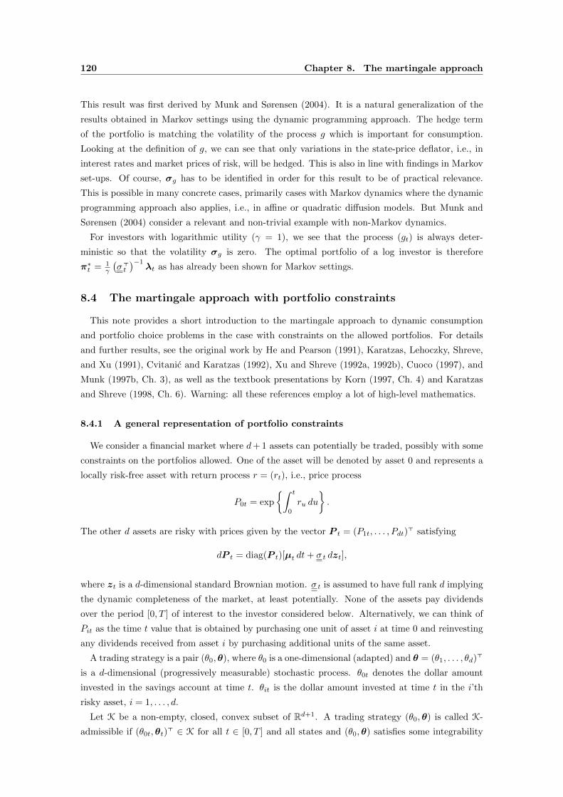
120 Chapter 8. The martingale approach
This result was first derived by Munk and Sørensen (2004). It is a natural generalization of the
results obtained in Markov settings using the dynamic programming approach. The hedge term
of the portfolio is matching the volatility of the process g which is important for consumption.
Looking at the definition of g, we can see that only variations in the state-price deflator, i.e., in
interest rates and market prices of risk, will be hedged. This is also in line with findings in Markov
set-ups. Of course, σg has to be identified in order for this result to be of practical relevance.
This is possible in many concrete cases, primarily cases with Markov dynamics where the dynamic
programming approach also applies, i.e., in affine or quadratic diffusion models. But Munk and
Sørensen (2004) consider a relevant and non-trivial example with non-Markov dynamics.
For investors with logarithmic utility (γ = 1), we see that the process (gt) is always deter-
ministic so that the volatility σg is zero. The optimal portfolio of a log investor is therefore
π∗t = 1γ
(σ>t
)−1λt as has already been shown for Markov settings.
8.4 The martingale approach with portfolio constraints
This note provides a short introduction to the martingale approach to dynamic consumption
and portfolio choice problems in the case with constraints on the allowed portfolios. For details
and further results, see the original work by He and Pearson (1991), Karatzas, Lehoczky, Shreve,
and Xu (1991), Cvitanic and Karatzas (1992), Xu and Shreve (1992a, 1992b), Cuoco (1997), and
Munk (1997b, Ch. 3), as well as the textbook presentations by Korn (1997, Ch. 4) and Karatzas
and Shreve (1998, Ch. 6). Warning: all these references employ a lot of high-level mathematics.
8.4.1 A general representation of portfolio constraints
We consider a financial market where d+ 1 assets can potentially be traded, possibly with some
constraints on the portfolios allowed. One of the asset will be denoted by asset 0 and represents a
locally risk-free asset with return process r = (rt), i.e., price process
P0t = exp
∫ t
0
ru du
.
The other d assets are risky with prices given by the vector P t = (P1t, . . . , Pdt)> satisfying
dP t = diag(P t)[µt dt+ σ t dzt],
where zt is a d-dimensional standard Brownian motion. σ t is assumed to have full rank d implying
the dynamic completeness of the market, at least potentially. None of the assets pay dividends
over the period [0, T ] of interest to the investor considered below. Alternatively, we can think of
Pit as the time t value that is obtained by purchasing one unit of asset i at time 0 and reinvesting
any dividends received from asset i by purchasing additional units of the same asset.
A trading strategy is a pair (θ0,θ), where θ0 is a one-dimensional (adapted) and θ = (θ1, . . . , θd)>
is a d-dimensional (progressively measurable) stochastic process. θ0t denotes the dollar amount
invested in the savings account at time t. θit is the dollar amount invested at time t in the i’th
risky asset, i = 1, . . . , d.
Let K be a non-empty, closed, convex subset of Rd+1. A trading strategy (θ0,θ) is called K-
admissible if (θ0t,θt)> ∈ K for all t ∈ [0, T ] and all states and (θ0,θ) satisfies some integrability

8.4 The martingale approach with portfolio constraints 121
conditions ensuring that the value of the trading strategy is well-defined. K is called the portfolio
constraint set. Various interesting specifications of K are listed below. The set of K-admissible
trading strategies is denoted by P(K). A consumption process is a non-negative (progressively
measurable) process c in L1[0, T ]. The set of consumption processes is denoted by C.
Given a trading strategy (θ0,θ) ∈ P(K) and a consumption process c ∈ C, the dynamics of the
investor’s wealth Wt = W θ0,θ,ct is
dWt =[θ0t rt + θ>
t µt + yt − ct]dt+ θ>
t σ t dzt. (8.12)
Initial wealth is W0 = w. Here y is a non-negative (progressively measurable) stochastic process
representing the endowment stream of the agent, e.g., labor income. Since θ0t = Wt− θ>
t 1, we can
rewrite the wealth dynamics as
dWt = [rtWt + θ>t (µt − rt1) + yt − ct] dt+ θ>
t σ t dzt,
which does not involve θ0 explicitly. Note, however, that there may be constraints on the investment
in the instantaneously risk-free asset.
A triple (θ0,θ, c) is called K-admissible given the initial wealth w if
(i) (θ0,θ) ∈ P(K), c ∈ C,
(ii) W θ0,θ,ct ≥ −K at all times t ∈ T for some positive constant K,
(iii) W θ0,θ,cT ≥ 0.
Let A(w;K) denote the set of triples (θ0,θ, c), which are K-admissible with initial wealth w.
In some situations, it is advantageous to let the agent choose a terminal wealth W directly
instead of choosing a trading strategy (θ0,θ). A consumption/terminal wealth pair (c,W ), where
c ∈ C and W is a non-negative FT -measurable random variable with finite expectations, is called
K-admissible with initial wealth w, if there exists a trading strategy (θ0,θ) such that (θ0,θ, c) is
K-admissible with W θ0,θ,c0 = w and W θ0,θ,c
T = W . In that case (θ0,θ) is said to finance (c,W ).
Let A′(w;K) denote the set of K-admissible consumption/terminal wealth pairs (c,W ). Clearly, if
(θ0,θ, c) ∈ A(w;K), then (c,W θ0,θ,cT ) ∈ A′(w;K).
Note that we can model situations, where the endowment stream is not spanned by traded assets,
i.e., where y is not adapted to the filtration generated by traded assets, by letting y depend on,
say, Pd and then restricting the investor to a policy with values in (a subset of) R× Rd−1 × 0.By restricting the individuals to K-admissible processes, a number of interesting situations can
be examined. It turns out that the so-called support function of −K plays an important role. Let
ν = (ν0,ν) ∈ R× Rd. Then the support function δ : Rd+1 → R ∪ −∞,+∞ of −K is defined by
δ(ν) = sup(θ0,θ)∈K
(−θ0ν0 − θ>ν) .
The effective domain of δ, i.e. the set of ν ∈ Rd+1 for which δ(ν) < ∞, is denoted by K. Next,
we list a few interesting properties of δ and K. See, e.g., Rockafellar (1970, Sect. 13) for more on
support functions.
(i) K is a closed convex cone2, called the barrier cone of −K.
2A set D ⊆ RN is called a cone if αx ∈ D whenever x ∈ D and α > 0.

122 Chapter 8. The martingale approach
(ii) If K is a cone, then δ ≡ 0 on K.
(iii) δ is sub-additive, that is
δ(ν1) + δ(ν2) ≥ δ(ν1 + ν2),
which follows from the corresponding property of the supremum operator.
(iv) If (θ0,θ) ∈ K and ν ∈ K, then
θ0ν0 + θ>ν + δ(ν) ≥ 0. (8.13)
Of course, this follows trivially from the definition of δ.
It turns out that we need to impose the following assumption on K.
Assumption 8.1. K is such that δ is bounded from above on K, or, equivalently, δ is non-positive
on K and ν0 ≥ 0 for all ν ∈ K.
Note that we are considering constraints on the amounts invested in the different assets. Cvitanic
and Karatzas (1992) started all this, but considered constraints on portfolio weights, which is less
general than constraints on amounts invested. Munk (1997b) extended/adapted the results of
Cvitanic and Karatzas (1992) to constraints on amounts invested, which is particularly important
to cover labor income where portfolio weights might not be well-defined. Here are examples of
interesting constraint sets:
Example 8.1. [Complete market] A complete market corresponds to having K = Rd+1. This
implies that K = 0d+1 and δ(ν) = 0 for all ν ∈ K. This is the standard market structure,
in which (in various degrees of generality) consumption/portfolio problems are studied by, e.g.,
Merton (1969, 1971), Karatzas, Lehoczky, and Shreve (1987), and Cox and Huang (1989, 1991).
2
Example 8.2. [Non-traded assets] A situation where there are only m < d tradable risky assets,
but otherwise no constraints on the tradable assets, can be modeled by letting K = R × Rm ×0d−m. In that case, K = 0 × 0m × Rd−m and δ(ν) = 0 on K. 2
Example 8.3. [Short-sale constraints] To model prohibition of short-selling the risky assets number
m+ 1, . . . , d, let K = R×Rm ×Rd−m+ . Then K = 0× 0m ×Rd−m+ and again δ(ν) = 0 on K.
2
Example 8.4. [Buying constraints] With K = R × Rm × Rd−m− , the investor is not allowed to
have positive amounts invested in the last d−m risky assets. Then K = 0 × 0m ×Rd−m− and
δ(ν) = 0 on K. 2
Example 8.5. [Portfolio mix constraints] K = (θ0,θ) ∈ Rd+1 | x ≡ θ0 +θ>1 ≥ 0 and π ∈ K(x),where K(x) is some non-empty, closed, convex subset of Rd containing the origin, and vπ = θ/x

8.4 The martingale approach with portfolio constraints 123
for x > 0 and vπ = 0 for x = 0, models a portfolio mix constraint. In this case
K = ν ∈ Rd+1 | ν>(θ0,θ) ≥ 0, ∀(θ0,θ) ∈ K
and δ(ν) = 0 on K. 2
Example 8.6. [Collateral constraints] With K =
(θ0,θ) ∈ Rd+1∣∣ψ>(θ0,θ) ≥ 0
, where ψ ∈
[0, 1]d+1, we can model the situation, where, using the j’th security (j = 0, 1, . . . , d) as collateral,
it is only possible to borrow the fraction ψj of its value. In this case K = ψR+ = kψ|k ≥ 0 and
δ(ν) = 0 on K. 2
Example 8.7. [Minimum capital requirements] Let K = (θ0,θ) ∈ Rd+1 | θ0 + θ>1 ≥ k, where
k ∈ R+. Then K = R+1d+1 = (ψ, . . . , ψ) ∈ Rd+1 | ψ ≥ 0, and δ(ν) = −kν0 for ν = (ν0,ν) ∈ K.
The special minimum capital requirement k = 0 represents a borrowing constraint. 2
Example 8.8. [Combinations of constraints] Any combination of the above constraints, i.e., where
K is the intersection of some of the K’s of the previous examples. 2
8.4.2 The problem to solve
The general utility maximization problem to solve is
J(w) = sup(θ0,θ,c)∈A(w;K)
V θ0,θ,c(w),
where
V θ0,θ,c(w) = E
[∫ T
0
U1(cs, s) ds+ U2(W θ0,θ,cT , T )
]and it is understood that the wealth process starts at W θ0,θ,c
0 = w. Equivalently, we can solve
J(w) = sup(c,W )∈A′(w;K)
V c,W (w),
where
V c,W (w) = E
[∫ T
0
U1(cs, s) ds+ U2(W,T )
].
We assume that the utility functions U1(·, t) and U2(·, T ) have infinite marginal utility at zero, i.e.,
U ′1(0, t) ≡ limc↓0 U′1(c, t) = ∞ and similarly U ′2(0, T ) ≡ limW↓0 U
′2(W,T ) = ∞. A technical aside:
we have to modify the definition of the set of admissible policies such that now A(w;K) denotes
the set of strategies (θ0,θ, c) which are admissible in the sense explained above and, further, satisfy
the condition3
E
[∫ T
0
U1(ct, t)− dt+ U2(W θ0,θ,c
T , T )−
]<∞
and similarly for A′(w;K).
3Here X− = max0,−X.

124 Chapter 8. The martingale approach
8.4.3 Auxiliary unconstrained problems
We will define a set of artificial, auxiliary unconstrained markets. Given a process (ν0,ν), where
(ν0t,νt) ∈ K for any t ∈ [0, T ], we define a market Mν where the short-term risk-free rate, the
expected returns on the risky assets, and the income rate are perturbed relative to the true market:
(i) the risk-free rate at time t is rt + ν0t,
(ii) the drift vector of the risky asset prices is µt + νt,
(iii) the income rate is yt + δ(νt).
There are no portfolio constraints in the artificial market Mν , i.e., it is a complete market. The
unique market price of risk is
λνt = σ−1t (µt + νt − (rt + ν0t)1),
the change of measure to the unique risk-neutral measure Qν is captured by dQνdP = ZνT , where
Zνt = exp
−∫ t
0
λ>νs dzs −
1
2
∫ t
0
λ>νsλνs ds
,
and the unique state-price deflator is given by
ζνt = exp
−∫ t
0
(rs + ν0s)) ds
Zνt.
In general, Zν is a local martingale. For technical reasons, we have to restrict ourselves to ν’s for
which Z is a true martingale. Let N∗ be the set of such processes ν, i.e.,
N∗ =ν ∈ L2[0, T ]
∣∣∣ν(t, ω) ∈ K, ∀(t, ω) ∈ [0, T ]× Ω and Zν is a martingale.
The wealth process in the auxiliary market Mν corresponding to any investment/consumption
policy (θ0,θ, c) is the process W θ0,θ,cν given by
dW θ0,θ,cνt = (θ0t[rt + ν0t] + θ>
t [µt + νt]) dt− (ct − yt − δ(νt)) dt+ θ>t σ t dzt
= (θ0trt + θ>t µt) dt− (ct − yt) dt+ θ>
t σ t dzt + (δ(νt) + θ0tν0t + θ>t νt) dt.
(8.14)
Note that, from (8.13),
δ(νt) + θ0tν0t + θ>t νt ≥ 0,
so a comparison of (8.14) and (8.12) yields that
W θ0,θ,cνt ≥W θ0,θ,c
t (8.15)
path-by-path: following a given strategy you will always end up with at least as high a terminal
wealth in any artificial market as in the true market.
A triple (θ0,θ, c) consisting of a trading strategy (θ0,θ) and a consumption process c is called
admissible in Mν [with initial wealth w] if (θ0,θ, c) and W θ0,θ,cν satisfy the same conditions as a
K-admissible triple in the original market except for the requirement (θ0t,θt) ∈ K, ∀t. The set of

8.4 The martingale approach with portfolio constraints 125
triples (θ0,θ, c) admissible in Mν is denoted Aν(w), i.e.,
Aν(w) =
(θ0,θ, c) ∈ P(Rd+1)× C
∣∣∣∣∣W θ0,θ,cνt ≥ −K, t ∈ [0, T ], W θ0,θ,c
νT ≥ 0, and
E
[∫ T
0
U1(ct, t)− dt+ U2(W θ0,θ,c
νT , T )−
]<∞
.
The unconstrained utility maximization problem in Mν is
Jν(w) = sup(θ0,θ,c)∈Aν(w)
V θ0,θ,c(w).
We let (θν0 ,θν , cν) denote the optimal strategy in the market Mν , i.e., Jν(w) = V θ
ν0 ,θ
ν ,cν (w). As
before, we can also maximize over consumption and terminal wealth:
Jν(w) = sup(c,W )∈A′ν(w)
V c,W (w).
Let (cν ,W ν) denote the optimal consumption process and terminal wealth in the market Mν , i.e.,
Jν(w) = V cν ,W ν
(w). Admissibility means budget-feasible in the sense that
E
[∫ T
0
ζνt (ct − yt − δ(νt)) dt+ ζνTW
]≤ w,
plus some technical integrability conditions.
8.4.4 Linking the artificial markets to the true market
Due to (8.15), we can conclude that (θ0,θ, c) ∈ A(w;K)⇒ (θ0,θ, c) ∈ Aν(w). Consequently,
J(w) ≤ Jν(w), ∀ν ∈ N∗. (8.16)
The indirect utility obtainable in any of the artificial markets is at least as high as the indirect
utility in the true market. The main result of Cvitanic and Karatzas (1992) and Munk (1997b,
Ch. 3) is to provide the following four ways to characterize optimality in the true market via the
artificial markets:
1. Minimality of ν: The optimal trading strategy in an artificial market is not necessarily
K-valued and is therefore not necessarily admissible in the true market. If we can find an
artificial market Mν in which the optimal strategy (θν0 ,θν , cν) is also admissible in the true
market, then it is clear that
J(w) ≥ V θν0 ,θ
ν ,cν (w) = Jν(w).
Combining that with (8.16), we can conclude that
J(w) = Jν(w) = V θν0 ,θ
ν ,cν (w)
so that (θν0 ,θν , cν) is the optimal strategy also in the true market. It is clear that J(w) =
Jν(w) can only be satisfied in the the least favorable artificially unconstrained market, i.e.,
we should minimize the indirect utility over all artificial markets.

126 Chapter 8. The martingale approach
2. Financiability of (cν ,W ν): Suppose we can find a ν so that the optimal consumption and
terminal wealth (cν ,W ν) is financed by a trading strategy (θν0 ,θν), which is K-valued and
satisfies
δ(νt) + θν0tν0t + (θνt )>νt = 0
for all t and all states. Then it follows from (8.14) that the strategy will generate the same
terminal wealth in the true market as in the artificial market Mν . Since the strategy is
admissible in the true market, we have
J(w) ≥ V θν0 ,θ
ν ,cν (w) = Jν(w),
and again we can combine that with (8.16) and conclude that (θν0 ,θν , cν) is optimal in the
true market.
3. Parsimony of ν: If we can find a ν ∈ N∗ such that (cν ,W ν) ∈ C× L1+ satisfies
E
[∫ T
0
ζνt (cνt − yt − δ(νt)) dt+ ζνTWν
]≤ w, ∀ν ∈ N∗,
then (cν ,W ν) and the corresponding strategy (θν0 ,θν , cν) are optimal in the true market.
This proof is complicated and will be skipped here. Note that the left-hand side of the above
inequality is the cost of implementing (cν ,W ν) in the artificial market Mν . For ν = ν,
the above inequality will be satisfied as an equality. The intuition is that if we can find
an artificial market for which the optimal strategy is budget-feasible in all other artificial
markets, then it is the least expensive and hence the least favorable of the solutions to the
artificial market problems.
4. Dual optimality of ν: The unconstrained maximization problem
Jν(w) = sup(c,W )
E
[∫ T
0
U1(cs, s) ds+ U2(W,T )
],
s.t. E
[∫ T
0
ζνt (ct − yt − δ(νt)) dt+ ζνTW
]≤ w,
can be solved with Lagrangian technique. If ψ denotes the Lagrange multiplier on the budget
constraint, the solution can be written as ct = I1(ψζνt, t), W = I2(ψζνT , T ), where I1(·, t)and I2(·, T ) are the inverse functions of U ′1(·, t) and U2(·, T ), respectively. Substituting the
solution back into the objective function, we obtain V ν(ψ) + ψw, where
V ν(ψ) = E
[∫ T
0
U1(ψζνt, t) dt+ U2(ψζνT , T )
]+ ψE
[∫ T
0
ζνt (yt + δ(νt) dt
],
and U1 and U2 are the convex conjugates of U1 and U2, respectively, i.e.
U1(x, t) = supq>0U1(q, t)− qx = U1(I1(x, t), t)− xI1(x, t),
and similarly for U2. The problem
J(ψ) = infν∈N∗
V ν(ψ)

8.5 Exercises 127
is called the dual problem. The Lagrange multiplier in Mν is related to initial wealth w via
some function ψ = Yν(w) which ensures that the budget constraint is satisfied as an equality.
It can then be shown that the dual problem is linked to the original problem as follows: if
we can find a ν ∈ N∗ such that
J(ψ) = V ν(ψ) for ψ = Yν(w),
then Mν is the least favorable market and (θν0 ,θν , cν) is optimal for the original constrained
problem in the true market.
The dual problem leads to a way of proving the existence of an optimal consumption and
investment strategy in the constrained true market. If there is a solution to the dual problem, then
there is also a solution to the primal problem, i.e., the utility maximization problem in the true
market. Cvitanic and Karatzas (1992) state sufficient conditions for the existence of an optimal
solution to the dual problem, which are then also sufficient conditions for the existence of an
optimal consumption and investment strategy in the constrained true market. However, one of
the conditions is that the Arrow-Pratt relative risk aversion measures corresponding to the utility
functions U1 and U2 are smaller than or equal to one, whereas individuals are generally believed to
have a relative risk aversion greater than one. Cuoco (1997) attacks the primal problem directly
using alternative methods and is able to establish less restrictive conditions for the existence of an
optimal solution.
The results above provide important intuition for constrained utility maximization problems.
The results have been used to provide explicit solutions to some constrained utility maximization
problems, but only with simple constraints and simple preferences such as logarithmic utility. The
ideas of considering the dual problem and the artificially unconstrained markets have also been
used recently in various numerical solution techniques, cf. Haugh, Kogan, and Wang (2006) and
Bick, Kraft, and Munk (2012).
8.5 Exercises
Exercise 8.1. Show that (8.2) follows from (8.1).


CHAPTER 9
Numerical methods for solving dynamic asset allocation problems
If the problem features CRRA utility, no portfolio constraints, and return dynamics that do not
fit into neither the affine nor the quadratic class: with (i) utility of terminal wealth only or (ii)
complete markets and utility of intermediate consumption and/or terminal wealth, it suffices to
solve a PDE like (7.40) numerically. This can be done (when the dimension of the state variable is
three or lower) using standard methods, like finite difference methods. See, e.g., Wilmott, Dewynne,
and Howison (1993), Thomas (1995), Wilmott (1998), Tavella and Randall (2000), Seydel (2009),
and Munk (2011). With incomplete markets and intermediate consumption, the more complicated
PDE (7.39) has to be solved numerically. For more general preferences, we would normally have
to solve the even more complicated PDE (7.9) numerically.
In many realistic cases, the portfolios are constrained and these constraints have to be taken into
account when solving the HJB equation, and then closed-form solutions are generally impossible
to find. It is still possible (at least, for low-dimensional problems) to implement a finite difference
type recursive solution method to solve the relevant HJB equation (a variant is called the Markov
Chain Approximation Approach). See, e.g., Brennan, Schwartz, and Lagnado (1997), Fitzpatrick
and Fleming (1991), Munk (1997a, 2003), Van Hemert (2010), and Munk and Sørensen (2010). A
more or less equivalent approach used in some papers is to assume a discrete-time setting from
the beginning and then solve the Bellman equation by backwards recursive dynamic programming.
However, some authors use large time steps (e.g., allow only annual consumption and investment
decisions) and assume very simple distributions (binomial, trinomial) of the relevant state variables
over these long time steps. See, e.g., Campbell and Cocco (2003), Cocco (2005), Cocco, Gomes,
and Maenhout (2005), and Yao and Zhang (2005a).
An alternative which, at least potentially, can handle higher-dimensional problems is Monte
Carlo simulation based approaches to the HJB equation. Various versions have been proposed.
See, e.g., Detemple, Garcia, and Rindisbacher (2003, 2005), Cvitanic, Goukasian, and Zapatero
(2003), Brandt, Goyal, Santa-Clara, and Stroud (2005), van Binsbergen and Brandt (2007), and
Koijen, Nijman, and Werker (2007, 2010).
129

130 Chapter 9. Numerical methods for solving dynamic asset allocation problems
Yet another alternative for the solution of some consumption and portfolio choice problems
involving portfolio constraints and/or incomplete markets is suggested by Bick, Kraft, and Munk
(2012). The method applies to CRRA utility and return dynamics of the affine-quadratic type.
The method combines (i) the idea of artificially unconstrained and complete markets introduced in
connection with the martingale approach in Section 8.4 and (ii) the results on closed-form solutions
for unconstrained affine-quadratic settings and CRRA utility. The method considers a subset of
artificially unconstrained and complete markets for which relatively simple closed-form solutions
exists. Each of these strategies is transformed into a feasible strategy in the true, constrained
market. This gives a set of feasible strategies parameterized by a number of parameters. If this
number is fairly low, one can search for the best of the strategies, where the evaluation of the
strategy is done via Monte Carlo simulation. The method also provides an upper bound for the
true, unknown optimal expected utility (given by the worst of the considered artificial markets)
and thus an upper bound on the wealth-equivalent loss the individual might suffer by following the
best of the feasible strategies considered. Another numerical method building on the martingale
techniques was suggested by Haugh, Kogan, and Wang (2006).

CHAPTER 10
Asset allocation with stochastic interest rates
10.1 Introduction
It is an empirical fact that both nominal and real interest rates and bond yields vary stochasti-
cally over time. It is therefore natural to include the short-term interest rate rt as a state variable.
This was first done in a portfolio-choice context by Merton (1973b) who considered a general
one-factor dynamics for rt, but he was not able to go beyond the general characterization of the
investment strategy in (7.7). We will focus on individuals with CRRA utility and on models in
which the interest rate dynamics is of an affine form, since then we can obtain closed-form solutions
for the optimal strategies as explained in Section 7.3.2. The affine class includes the well-known
models of Vasicek (1977) and Cox, Ingersoll, and Ross (1985). See, e.g., Munk (2011) for a com-
prehensive analysis of dynamic models of the term structure of interest rates. We can also apply
the general results of Section 7.3 to cases where the dynamics of the term structure of interest rate
is given by a multi-factor affine or quadratic model.
Recall that investors are (or should be) concerned about real interest rates and hence they
would want to invest in real bonds. Indeed, we will assume that investors have access to trade
in a complete market of real bonds (Exercise 10.1 at the end of the chapter discusses an optimal
investment problem with stochastic interest rates when no bonds are traded.) We will focus on
determining the optimal bond/stock mix so we assume that only a single stock is traded. We
interpret this stock as the entire stock market index. The results can be generalized to the case
with multiple stocks.
Investors with non-log utility will hedge variations in interest rates. Bonds carry a build-in hedge
against interest rate risk since bond prices are inversely related to interest rates. Over a period
where interest rates have fallen, indicating that future investment opportunities are worsened, bond
prices have risen and generated a positive return. The converse is also true. We will therefore
expect that interest rates are hedged by investing in bonds, but precisely how many bonds and
which bonds this hedge should involve has to be computed using concrete models.
In Section 10.2 we study the case where the real short-term interest rate behaves according to
131

132 Chapter 10. Asset allocation with stochastic interest rates
the Vasicek model. Section 10.3 considers the CIR model of interest rates. Section 10.4 gives
a numerical example in which the quantitative effects of interest rate uncertainty on optimal
portfolios can be assessed. Section 10.5 briefly looks at optimal portfolio choice when interest rate
dynamics is given by a two-factor version of the Vasicek model. Other studies with stochastic
interest rates are briefly discussed in Section 10.6. In many countries there are no liquid markets
for real bonds, only for nominal bonds. Then we have to take the dynamics of consumer prices
and inflation into account. We consider those issues in Chapter 12.
10.2 One-factor Vasicek interest rate dynamics
Following Vasicek (1977), assume that rt follows the Ornstein-Uhlenbeck process
drt = κ[r − rt] dt− σr dz1t,
with an associated constant market price of risk λ1. We assume that κ, r, and σ are positive
constants. The process exhibits mean reversion in the sense that, if rt < r, the short rate is
expected to increase over the next instant, whereas if rt > r, the short rate is expected to fall.
This is a very realistic feature of the model. Future values of the short rate are normally distributed
so, in particular, short rates can take on any negative value, which is not realistic.
It is a consequence of these assumptions that the price of a zero-coupon bond with maturity T
is given by
BTt = e−a(T−t)−b(T−t)rt ,
where
b(τ) =1
κ
(1− e−κτ
),
a(τ) = y∞ (τ − b(τ)) +σ2r
4κb(τ)2,
where y∞ =(r + λ1σr
κ − σ2r
2κ2
)is the asymptotic zero-coupon yield as time-to-maturity goes to
infinity. From Ito’s Lemma it follows that the dynamics of the zero-coupon bond price is
dBTt = BTt[(rt + λ1σrb(T − t)
)dt+ σrb(T − t) dz1t
],
and similarly the dynamics of any bond (or any other fixed-income security) is of the form
dBt = Bt [(rt + λ1σB(rt, t)) dt+ σB(rt, t) dz1t] . (10.1)
It is well-known that any bond (or other fixed-income security) can be generated from an appro-
priate dynamic investment strategy in the bank account and in just one (arbitrary) bond (or other
long-lived term structure derivative). Let us for the present take an arbitrary bond with price Bt
and dynamics given by (10.1).
The price of the single stock (representing the stock market index) is assumed to follow the
process
dSt = St
[(rt + ψσS) dt+ ρσS dz1t +
√1− ρ2σS dz2t
].
The parameter ρ is the correlation between bond market returns and stock market returns, σS is
the volatility of the stock, and ψ is the Sharpe ratio of the stock which we assume constant.

10.2 One-factor Vasicek interest rate dynamics 133
The asset allocation problem of a CRRA investor under these assumptions was studied by
Sørensen (1999) and Bajeux-Besnainou, Jordan, and Portait (2001) for utility of terminal wealth
only. Korn and Kraft (2001) discuss some technical issues related to the application of the verifi-
cation theorem to this problem.
To get this into the notation applied so far, we rewrite the price dynamics as(dBt
dSt
)=
(Bt 0
0 St
)[(rt1 +
(σB(rt, t) 0
ρσS√
1− ρ2σS
)(λ1
λ2
))dt
+
(σB(rt, t) 0
ρσS√
1− ρ2σS
)(dz1t
dz2t
)],
where
λ2 = (ψ − ρλ1)/√
1− ρ2. (10.2)
We are therefore in a complete market model with a single state variable (x = r). We can rewrite
the dynamics of r as
drt = κ[r − rt] dt+(−σr, 0
)dzt,
where z = (z1, z2)>. In this model the state variable has an affine drift and a constant volatility,
and the market price of risk vector λ = (λ1, λ2)> is also constant. Hence, Theorem 7.7 applies
with CRRA utility from terminal wealth only and Theorem 7.8 applies with CRRA utility from
intermediate consumption and possibly terminal wealth. In the notation used there, we have
r0 = 0, r1 = 1, m0 = κr, m1 = −κ,
Λ0 = λ21 + λ2
2, Λ1 = 0, v0 = 0, v1 = 0,
V0 = σ2r , V1 = 0, K0 = −σrλ1, K1 = 0.
In this case the ordinary differential equation (7.22) reduces to
A′1(τ) = 1− κA1(τ),
which with the initial condition A1(0) = 0 has the unique solution
A1(τ) =1
κ
(1− e−κτ
)= b(τ).
This result also follows from the discussion below Theorem 7.7. Next, A0 follows from (7.25):
A0(τ) =1
2γ
(λ2
1 + λ22
)τ +
(κr +
γ − 1
γσrλ1
)∫ τ
0
b(s) ds− γ − 1
2γσ2r
∫ τ
0
b(s)2 ds
=1
2γ
(λ2
1 + λ22
)τ +
(r − γ − 1
2κ2γ
[σ2r − 2κσrλ1
])(τ − b(τ)) +
γ − 1
4κγσ2rb(τ)2,
where we have used that∫ τ
0
b(s) ds =1
κ(τ − b(τ)) ,
∫ τ
0
b(s)2 ds =1
κ2(τ − b(τ))− 1
2κb(τ)2.
For the case with utility from terminal wealth only we have from Theorem 7.7 that the optimal
investment strategy is
Π(W, r, t) ≡
(ΠB(W, r, t)
ΠS(W, r, t)
)=
1
γ
(σ (r, t)>
)−1λ− γ − 1
γ
(σ (r, t)>
)−1
(−σr
0
)b(T − t)
=1
γ
(σ (r, t)>
)−1λ+
γ − 1
γ
(σ (r, t)>
)−1
(σr
0
)b(T − t).
(10.3)

134 Chapter 10. Asset allocation with stochastic interest rates
We can see that the hedge portfolio only involves the bond, not the stock, which should not come
as a surprise since bonds seem more appropriate for hedging interest rate risk than stocks. The
higher the risk aversion γ, the lower the investment in the tangency portfolio and the higher the
investment in the hedge bond. The inverse of the transposed volatility matrix is(σB(r, t) ρσS
0√
1− ρ2σS
)−1
=1√
1− ρ2σB(r, t)σS
(√1− ρ2σS −ρσS
0 σB(r, t)
)
so that we can write out the fraction of wealth invested in the stock and the bond as
ΠS(W, r, t) =λ2
γσS√
1− ρ2, (10.4)
ΠB(W, r, t) =1
γσB(r, t)
(λ1 −
ρ√1− ρ2
λ2
)+γ − 1
γ
σrb(T − t)σB(r, t)
. (10.5)
If the bond in the portfolio is the zero-coupon bond maturing at the end of the investment
horizon of the investor, i.e., at time T , then σB(r, t) = σrb(T − t), and we see that the hedge term
simply consists of a fraction (γ − 1)/γ in the zero-coupon bond. This is a natural choice of hedge
instrument since it is exactly the truly risk-free asset for an investor only interested in time T
wealth. The log utility investor (γ = 1) does not hedge. The hedge position of a less risk averse
investor (γ < 1) is negative, while a more risk averse investor (γ > 1) takes a long position in the
bond in order to hedge interest rate risk. An infinitely risk averse investor (γ →∞) will invest her
entire wealth in the zero-coupon bond maturing at T .
If we continue to use the zero-coupon bond maturing at T as the bond instrument, we see
from (10.3) that we can write the risky part of the optimal investment strategy as
Π(W, r, t) ≡
(ΠB(W, r, t)
ΠS(W, r, t)
)=
1
γ
(σ (t)>
)−1λ+
γ − 1
γ
(1
0
).
Consequently, the fraction of wealth invested in the bank account (i.e., the locally risk-free asset)
is
Π0(W, r, t) = 1−ΠB(W, r, t)−ΠS(W, r, t)
= 1− 1
γ1>(σ (t)>
)−1λ− γ − 1
γ
=1
γ
(1− 1>
(σ (t)>
)−1λ).
Note that the term in the parenthesis is exactly what a log investor would hold in the bank account.
The entire investment strategy can be written asΠ0
ΠB
ΠS
=1
γ
Πlog
0
ΠlogB
ΠlogS
+γ − 1
γ
0
1
0
.
The strategy is hence a simple combination of the log investor’s portfolio and the zero-coupon bond
maturing at the investment horizon of the investor. Note that as the risk aversion γ increases, the
position in stocks will decrease, while the position in bonds will increase. Hence, the bond/stock
ratio increases with risk aversion consistent with popular advice. However, the allocation to stock

10.3 One-factor CIR dynamics 135
is still independent of the investment horizon which conflicts with traditional advice that the stock
weight should increase with the investment horizon.
With utility from intermediate consumption only, it follows from Theorem 7.8 that the hedge
term of the optimal bond investment strategy is
γ − 1
γ
σrσB(rt, t)
∫ Tte−
δγ (s−t)− γ−1
γ A0(s−t)− γ−1γ b(s−t)rb(s− t) ds∫ T
te−
δγ (s−t)− γ−1
γ A0(s−t)− γ−1γ b(s−t)r ds
, (10.6)
where σB(rt, t) again represents the volatility of the bond chosen for implementing the strategy.
It can be shown that the time t volatility of a coupon bond paying a continuous coupon at a
deterministic rate K(s) up to time T is given by
σB(r, t) =
∫ TtK(s)Bst σrb(s− t) ds∫ T
tK(s)Bst ds
.
Hence, we can interpret the time t interest rate hedge as the fraction (γ − 1)/γ of wealth invested
in a bond with continuous coupon
K(s) = ea(s−t)− γ−1γ A0(s−t)− δγ (s−t)+ 1
γ b(s−t)r.
Munk and Sørensen (2004) show that this coupon is closely related to the expected consumption
rate at time s. For an investor with utility from consumption over the entire period [t, T ], the zero-
coupon bond maturing at T is no longer the truly risk-free asset. Since the investor is interested
in payments at all dates in [t, T ], he hedges interest rate risk by investing in a combination of all
zero-coupon bonds maturing in this interval, i.e., in some sort of coupon bond.
10.3 One-factor CIR dynamics
Consider the same set-up as above except that the short-term interest rate now is assumed to
follow the square-root process
drt = κ[r − rt] dt− σr√rt dz1t, (10.7)
where κ, r, and σr are positive constants. The market price of the risk represented by z1 is assumed
to be given by λ1(r, t) = λ1√rt/σr. As shown by Cox, Ingersoll, and Ross (1985), zero-coupon
bond prices are on the form
BTt = e−a(T−t)−b(T−t)rt
as in the Vasicek model, but a and b are now given by
b(τ) =2(eατ − 1)
(α+ κ)(eατ − 1) + 2α,
a(τ) = −2κr
σ2r
(1
2(κ+ α)τ + ln
2α
(α+ κ)(eατ − 1) + 2α
),
where κ = κ− λ1 and α =√κ2 + 2σ2
r . The price evolves as
dBTt = BTt[(rt + b(T − t)λ1rt
)dt+ b(T − t)σr
√rt dz1t
].
We assume that the investor can also trade in a single stock with price St evolving as
dSt = St
[(rt + ψ(rt)σS) dt+ ρσS dz1t +
√1− ρ2σS dz2t
].

136 Chapter 10. Asset allocation with stochastic interest rates
Here σS is a positive constant, and z2 is a one-dimensional standard Brownian motion independent
of z1 so that the constant ρ is the instantaneous correlation between stock returns and bond returns.
We assume that the market price of risk associated with z2 is a constant λ2 so that
ψ(r) = ρλ1
σr
√r +
√1− ρ2λ2. (10.8)
Again we have an affine, complete market model of the type studied in Section 7.3.2. In this case
we have
r0 = 0, r1 = 1, m0 = κr, m1 = −κ,
Λ0 = λ22, Λ1 =
λ21
σ2r
, v0 = 0, v1 = 0,
V0 = 0, V1 = σ2r , K0 = 0, K1 = −λ1.
The solution is stated in terms of two deterministic functions A0 and A1. Let
κ = κ− γ − 1
γλ1.
The ordinary differential equation (7.22) for A1 becomes
A′1(τ) =
(1 +
λ21
2γσ2r
)− κA1(τ)− γ − 1
2γσ2rA1(τ)2
with the initial condition A1(0) = 0. Assuming
κ2 + 2σ2r
γ − 1
γ
(1 +
λ21
2γσ2r
)> 0,
which is certainly satisfied for γ ≥ 1, the unique solution is follows immediately from (7.24):
A1(τ) =2(
1 +λ2
1
2γσ2r
)(eντ − 1)
(ν + κ) (eντ − 1) + 2ν,
and we have introduced the additional auxiliary parameters
ν =
√κ2 + 2σ2
r
γ − 1
γ
(1 +
λ21
2γσ2r
).
A0 can then be computed from (7.25):
A0(τ) =λ2
2
2γτ + κr
∫ τ
0
A1(s) ds =λ2
2
2γτ − γ − 1
γ
2κr
σ2r
(1
2(ν + κ) τ + ln
2ν
(ν + κ) (eντ − 1) + 2ν
).
It follows from Theorem 7.7 that the optimal investment strategy for an investor with CRRA
utility from terminal wealth only is
ΠB(W, r, t) =1
γσB(r, t)
(λ1
σr
√r − ρλ2√
1− ρ2
)+γ − 1
γ
σr√r
σB(r, t)A1(T − t),
ΠS(W, r, t) =λ2
γσS√
1− ρ2.
If the bond instrument used is the zero-coupon bond maturing at the end of the investor’s horizon,
we have σB(r, t) = σr√rb(T − t), and the hedge component will simplify to γ−1
γ A1(t− t)/b(T − t).

10.4 A numerical example 137
As opposed to the Vasicek case we do not have A1(T − t) = b(T − t). This implies that the optimal
hedge consists of investing the time-varying fraction γ−1γ A1(T − t)/b(T − t) in the zero-coupon
bond maturing at the end of the investor’s horizon. A similar result was obtained by Deelstra,
Grasselli, and Koehl (2000) and Grasselli (2000) using the martingale approach for the case of
utility from terminal wealth only.
For an investor with CRRA utility of intermediate consumption only, Theorem 7.8 applies. The
fraction of wealth optimally invested in the stock is the same as above, while the fraction of wealth
optimally invested in the bond instrument changes to
ΠB(W, r, t) =1
γσB(r, t)
(λ1
σr
√r − ρλ2√
1− ρ2
)
+γ − 1
γ
σr√r
σB(r, t)
∫ TtA1(s− t)e−
δγ (s−t)− γ−1
γ A0(s−t)− γ−1γ A1(s−t)r ds∫ T
te−
δγ (s−t)− γ−1
γ A0(s−t)− γ−1γ A1(s−t)r ds
.
10.4 A numerical example
We will take historical estimates of mean returns, standard deviations, and correlations as rep-
resentative of future investment opportunities. These estimates are taken from Dimson, Marsh,
and Staunton (2002). All returns are measured per year. The historical average real return on
the U.S. stock market is µS = 8.7% with a standard deviation of σS = 20.2%, while the average
real return on bonds is µB = 2.1% with a standard deviation of σB = 10.0%. The average real
U.S. short-term interest rate is r = 1.0%. The correlation between stock returns and bond returns
is ρ = 0.2. Different bonds will have different average returns and different standard deviation of
the return. Similarly, the correlation between the return on a bond and the return on the stock
market index may not be identical for all bonds. It is not clear exactly what bond or bond index,
the above estimates are based on, but we will assume that the estimates for µB and σB apply to
a 10-year zero-coupon bond.
The volatility matrix of the bond and the stock is
σ =
(0.1 0
0.0404 0.1979
).
The (average) Sharpe ratio of the bond is λ1 = (2.1 − 1.0)/10.0 = 0.11 and the (average) Sharpe
ratio of the stock market is ψ = (8.7 − 1.0)/20.2 ≈ 0.3812. Using (10.2) this corresponds to a
market price of risk of λ2 ≈ 0.3666 on the exogenous shock that only affects the stock market. The
variance-covariance matrix of returns is Σ = σσ>. From (6.8), the tangency portfolio of the bond
and the stock is given by
πtan =
(πtanB
πtanS
)=
(0.1596
0.8404
),
so that the bond/stock ratio is approximately 0.19. Recall that this will be true for all agents who
have time-additive utility and who believe that investment opportunities are constant over time.
The tangency portfolio has a mean return of 7.65% and a standard deviation of 17.37%.
CRRA investors ignoring the fluctuations of interest rates will choose a portfolio of risky assets
given by π = 1γ [1>(σ>)−1λ]πtan, where γ is the relative risk aversion of the agent. The portfolio
is independent of the investment horizon. In Table 10.1 we show the portfolio allocation for

138 Chapter 10. Asset allocation with stochastic interest rates
γ tangency bond stock cash exp. return volatility
0.5 4.4079 0.7034 3.7045 -3.4079 0.3030 0.7655
1 2.2039 0.3517 1.8522 -1.2039 0.1565 0.3827
2 1.1020 0.1758 0.9261 -0.1020 0.0832 0.1914
2.2039 1.0000 0.1596 0.8404 0.0000 0.0765 0.1737
3 0.7346 0.1172 0.6174 0.2654 0.0588 0.1276
4 0.5510 0.0879 0.4631 0.4490 0.0466 0.0957
5 0.4408 0.0703 0.3704 0.5592 0.0393 0.0765
6 0.3673 0.0586 0.3087 0.6327 0.0344 0.0638
8 0.2755 0.0440 0.2315 0.7245 0.0283 0.0478
10 0.2204 0.0352 0.1852 0.7796 0.0246 0.0383
20 0.1102 0.0176 0.0926 0.8898 0.0173 0.0191
50 0.0441 0.0070 0.0370 0.9559 0.0129 0.0077
200 0.0110 0.0018 0.0093 0.9890 0.0107 0.0019
Table 10.1: Portfolio weights for CRRA investors ignoring interest rate fluctuations.
various γ-values. The numbers in the column “tangency” denotes the fraction of wealth invested
in the tangency portfolio. This investment is divided into the bond and the stock in the following
two columns. The cash position is determined residually so that weights sum to one. The last
two columns show the instantaneous expected rate of return and volatility of the portfolio. In
Figure 10.1 the curved line shows the mean-variance efficient portfolios of risky assets, i.e., the
combinations of expected returns and volatility that can be obtained by combining the bond and
the stock. The straight line corresponds to the optimal portfolios for investors assuming constant
investment opportunities with an interest rate equal to the long-term average.
Now let us look at investors who realize that interest rates vary over time and consequently
alter their investment strategy (except for log-utility investors). First, we assume that the real
short-term interest rate rt follows the one-factor Vasicek model so that the analysis and results
of Section 10.2 applies. The long-term average interest rate is r = 1.0% and we take a short-rate
volatility of σr = 5%, which is also consistent with the U.S. historical estimate. We use the same
values of the market prices of risk as above. We set the value of the mean reversion rate κ = 0.4965
so that the volatility of a 10-year zero-coupon bond according to the model is equal to the historical
estimate of 10.0%. The current short rate is assumed to equal the long-term level, rt = r.
Let us first consider investors with utility of terminal wealth only. Their optimal portfolios
are given by (10.4) and (10.5). Table 10.2 shows the optimal portfolios for CRRA investors with
different combinations of risk aversion and investment horizon. The numbers under the column
heading ‘hedge’ are γ−1γ b(T )/b(10), which is the hedge demand for the 10-year zero-coupon bond
which the investors are allowed to trade in. While the weight on the tangency portfolio and thus
the stock is independent on the investment horizon, this is not true for the weight on the hedge
portfolio and hence not true for the total weight on the bond and on cash. The ratio of the bond
weight to the stock weight is shown in the column ‘bond/stock’. The bond-stock ratio increases
considerably with the risk aversion and, for investors with γ > 1, with the investment horizon.
10.4 A numerical example 139
0%
2%
4%
6%
8%
10%
12%
14%
16%
0% 5% 10% 15% 20% 25% 30% 35% 40%
volatility
ex
p.
rate
of
retu
rn
Figure 10.1: The mean-variance frontiers. The figure shows the mean-variance frontier
without the risk-free asset (blue curve) and with the risk-free asset (straight black line). The
tangency portfolio of the risky assets is indicated with a red x.
The investor with a horizon of T will want to hedge interest rate risk by investing in the T -period
zero-coupon bond. That bond is replicated by a portfolio of b(T )/b(10) units of the 10-year zero-
coupon bond and a cash position. Since b is increasing in T , the hedge demand for the 10-year bond
increases with the horizon T . It is important to emphasize that the portfolio weights on the bond
and thus the bond/stock ratio will depend on the maturity (and payment schedule) of the bond, the
investor is trading in. In particular, a recommendation of a particular bond weight or bond/stock
ratio should always be accompanied by a specification of what bond the recommendation applies
to.
Next, we consider investors with utility from intermediate consumption and no utility from
terminal wealth. In this case the hedge term in the bond weight (10.5) is replaced by (10.6). Now
the hedge demand depends on the current interest rate level, which we assume is equal to the
long-term average of 1%. Table 10.3 shows the optimal portfolios for investors with a 1-year and a
30-year horizon. We see the same overall picture as for investors with utility from terminal wealth
only, but for a given investment horizon the hedge demand for bond and hence the bond/stock
ratio are smaller with utility of consumption since the optimal bond for hedging has a smaller
duration then the investment horizon.
Let us now compare the current mean/variance tradeoff chosen by different investors. As dis-
cussed above, CRRA investors that either have a zero (or very, very short) investment horizon or
do not take interest rate risk into account will pick a portfolio that corresponds to a point on the
straight line in Figure 10.2. This is the instantaneous mean-variance efficient frontier. Similarly,
each of the other curves corresponds to the combinations chosen by CRRA investors with a given

140 Chapter 10. Asset allocation with stochastic interest rates
horizon γ tangency hedge bond stock bondstock cash exp. return volatility
T = 1 0.5 4.4079 -0.3941 0.3093 3.7045 0.08 -3.0138 0.2986 0.7551
1 2.2039 0.0000 0.3517 1.8522 0.19 -1.2039 0.1565 0.3827
2 1.1020 0.1970 0.3729 0.9261 0.40 -0.2990 0.0854 0.1979
5 0.4408 0.3153 0.3856 0.3704 1.04 0.2439 0.0428 0.0908
10 0.2204 0.3547 0.3899 0.1852 2.11 0.4249 0.0286 0.0592
20 0.1102 0.3744 0.3920 0.0926 4.23 0.5154 0.0214 0.0467
T = 5 0.5 4.4079 -0.9229 -0.2195 3.7045 -0.06 -2.4850 0.2928 0.7442
1 2.2039 0.0000 0.3517 1.8522 0.19 -1.2039 0.1565 0.3827
2 1.1020 0.4615 0.6373 0.9261 0.69 -0.5634 0.0883 0.2094
5 0.4408 0.7383 0.8087 0.3704 2.18 -0.1791 0.0474 0.1207
10 0.2204 0.8306 0.8658 0.1852 4.67 -0.0510 0.0338 0.1010
20 0.1102 0.8768 0.8943 0.0926 9.66 0.0130 0.0270 0.0950
T = 10 0.5 4.4079 -1.0000 -0.2966 3.7045 -0.08 -2.4079 0.2920 0.7429
1 2.2039 0.0000 0.3517 1.8522 0.19 -1.2039 0.1565 0.3827
2 1.1020 0.5000 0.6758 0.9261 0.73 -0.6020 0.0887 0.2112
5 0.4408 0.8000 0.8703 0.3704 2.35 -0.2408 0.0481 0.1256
10 0.2204 0.9000 0.9352 0.1852 5.05 -0.1204 0.0345 0.1074
20 0.1102 0.9500 0.9676 0.0926 10.45 -0.0602 0.0278 0.1022
T = 30 0.5 4.4079 -1.0070 -0.3036 3.7045 -0.08 -2.4009 0.2919 0.7428
1 2.2039 0.0000 0.3517 1.8522 0.19 -1.2039 0.1565 0.3827
2 1.1020 0.5035 0.6794 0.9261 0.73 -0.6055 0.0888 0.2114
5 0.4408 0.8056 0.8760 0.3704 2.37 -0.2464 0.0482 0.1261
10 0.2204 0.9063 0.9415 0.1852 5.08 -0.1267 0.0346 0.1080
20 0.1102 0.9567 0.9743 0.0926 10.52 -0.0669 0.0278 0.1028
Table 10.2: Portfolio weights for CRRA investors who assume Vasicek interest rate
dynamics and have utility from terminal wealth only.

10.4 A numerical example 141
horizon γ tangency hedge bond stock bondstock cash exp. return volatility
T = 1 0.5 4.4079 -0.2253 0.4780 3.7045 0.1290 -3.1825 0.3005 0.7593
1 2.2039 0.0000 0.3517 1.8522 0.1899 -1.2039 0.1565 0.3827
2 1.1020 0.1114 0.2872 0.9261 0.3101 -0.2134 0.0845 0.1949
5 0.4408 0.1787 0.2490 0.3704 0.6722 0.3805 0.0413 0.0835
10 0.2204 0.2013 0.2365 0.1852 1.2766 0.5783 0.0269 0.0481
20 0.1102 0.2126 0.2302 0.0926 2.4856 0.6772 0.0197 0.0324
T = 30 0.5 4.4079 -0.9639 -0.2605 3.7045 -0.0699 -2.4440 0.2924 0.7435
1 2.2039 0.0000 0.3517 1.8522 0.1899 -1.2039 0.1565 0.3827
2 1.1020 0.4428 0.6187 0.9261 0.6677 -0.5448 0.0881 0.2085
5 0.4408 0.7254 0.7957 0.3704 2.1445 -0.1662 0.0473 0.1196
10 0.2204 0.8245 0.8597 0.1852 4.6319 -0.0449 0.0337 0.1004
20 0.1102 0.8751 0.8927 0.0926 9.6176 0.0147 0.0270 0.0948
Table 10.3: Portfolio weights for CRRA investors who assume Vasicek interest rate
dynamics and have utility from intermediate consumption only.
horizon tangency hedge bond stock bondstock cash exp. return volatility
T = 0 1.1020 0 0.1758 0.9261 0.19 -0.1020 0.0832 0.1914
T = 1, wealth 1.1020 0.1970 0.3729 0.9261 0.40 -0.2990 0.0854 0.1979
T = 5, wealth 1.1020 0.4615 0.6373 0.9261 0.69 -0.5634 0.0883 0.2094
T = 10, wealth 1.1020 0.5000 0.6758 0.9261 0.73 -0.6020 0.0887 0.2112
T = 30, wealth 1.1020 0.5035 0.6794 0.9261 0.73 -0.6055 0.0888 0.2114
T = 1, cons. 1.1020 0.1114 0.2872 0.9261 0.3101 -0.2134 0.0845 0.1949
T = 30, cons. 1.1020 0.4428 0.6187 0.9261 0.6677 -0.5448 0.0881 0.2085
Table 10.4: Portfolio weights for investors with a constant relative risk aversion of
γ = 2.
non-zero horizon who take interest rate risk into account. Since these curves lie to the right of
the instantaneous mean-variance frontier, all these investors could obtain a higher instantaneous
expected rate of return for the same volatility by choosing a different portfolio. But the long-term
investors are willing to sacrifice some expected return in the short term in order to hedge changes
in interest rates and place themselves in a better position if interest rates should decline.
Table 10.4 shows the optimal portfolios for investors with a constant relative risk aversion equal
to 2, but with different investment horizons. Here we can clearly see the effect of the investment
horizon on the optimal bond holdings and the bond/stock ratio. Relative to the extreme short-term
investor, long-term investors have the same stock weight but shifts wealth from cash to bonds. If
we look at the instantaneous risk/return trade-off, the longer-term investors choose more risky
portfolios, i.e., they take on more short-term risk. But the main point is that long-term investors
do not choose their portfolio according to the short-term risk/return trade-off.
Next, we want to investigate how sensitive the asset allocation choice is to the assumed interest

142 Chapter 10. Asset allocation with stochastic interest rates
0%
2%
4%
6%
8%
10%
12%
14%
16%
0% 5% 10% 15% 20% 25% 30% 35% 40%
volatility
exp
. ra
te o
f re
turn
Figure 10.2: Optimal frontiers with Vasicek interest rates. Each curve contains the
combinations of current expected rate of return and volatility for CRRA investors with a given
investment horizon T . From the left, the curves represent (a) T = 0 (black straight line; identical
to the mean-variance frontier), (b) T = 1 and utility of consumption (blue curve), (c) T = 1 and
utility from terminal wealth only (red cruve), (d) T = 30 and utility from consumption (grey
curve), and (e) T = 30 and utility from terminal wealth only (green curve).
rate model. We do that by computing the optimal portfolios when interest rates follow the CIR
model (10.7). We want to make a reasonably fair comparison between the two models. For that
purpose we choose σr = 0.5 in the CIR model so that the average short rate volatility is σr√r = 0.05
as in the Vasicek model. We set λ1 = 0.55 and λ2 = 0.3666 so that the model is consistent with
the estimated mean stock and bond returns when r = r is used to compute the Sharpe ratios of
the bond market (λ1(r)) and the stock market (ψ(r) in (10.8)). The mean reversion rate is set at
κ = 0.7994 so that the volatility of a 10-year zero-coupon bond according to the model is equal to
the historical estimate of 10.0%. The optimal portfolio in the CIR setting depends on the current
interest rate level. In the computations we put this equal to the long-term average of 1%.
In Table 10.5 we list the optimal portfolios for investors with CRRA utility of terminal wealth
both for the Vasicek and the CIR setting. We consider an investor with a 1-year horizon and
an investor with a 30-year horizon. The stock weight is identical in the two models. The hedge
demand for bonds and hence the total bond demand (and the cash position) do depend on the
interest rate model, but the differences are relatively small. The yield curves of the two models
are almost identical. The long-term yield is 1.601% in the Vasicek model and 1.600% in the CIR
model. With a current short rate of 1%, the yield curve is uniformly increasing in both models,
cf. the results on the shape of the yield curve in the two models reported by, e.g., Munk (2011).

10.5 Two-factor Vasicek model 143
Vasicek model CIR model
horizon γ tangency stock hedge bond cash hedge bond cash
T = 1 0.5 4.4079 3.7045 -0.3941 0.3093 -3.0138 -0.6374 0.0660 -2.7705
1 2.2039 1.8522 0.0000 0.3517 -1.2039 0 0.3517 -1.2039
2 1.1020 0.9261 0.1970 0.3729 -0.2990 0.2482 0.4241 -0.3502
5 0.4408 0.3704 0.3153 0.3856 0.2439 0.3653 0.4357 0.1939
10 0.2204 0.1852 0.3547 0.3899 0.4249 0.3979 0.4331 0.3817
20 0.1102 0.0926 0.3744 0.3920 0.5154 0.4129 0.4305 0.4769
T = 30 0.5 4.4079 3.7045 -1.0070 -0.3036 -2.4009 -1.0066 -0.3033 -2.4012
1 2.2039 1.8522 0.0000 0.3517 -1.2039 0 0.3517 -1.2039
2 1.1020 0.9261 0.5035 0.6794 -0.6055 0.5012 0.6771 -0.6032
5 0.4408 0.3704 0.8056 0.8760 -0.2464 0.8012 0.8715 -0.2420
10 0.2204 0.1852 0.9063 0.9415 -0.1267 0.9010 0.9362 -0.1214
20 0.1102 0.0926 0.9567 0.9743 0.0669 0.9509 0.9685 -0.0611
Table 10.5: Portfolio weights with Vasicek or CIR dynamics for CRRA investors
with utility from terminal wealth only.
10.5 Two-factor Vasicek model
Brennan and Xia (2000) study a two-factor Vasicek interest rate model with utility from terminal
wealth only. Assume that the dynamics of the short-term interest rate rt is
drt = (ϕr + ut − κrrt) dt− σr dz1t,
dut = −κuut dt− σuρru dz1t − σu√
1− ρ2ru dz2t,
where z1 = (z1t) and z2 = (z2t) are independent one-dimensional standard Brownian motions. The
one-factor Vasicek model is the special case where ut ≡ 0, and then the short rate rt is expected
to move towards the long-run level ϕr/κr. The new state variable u allows for variations in this
long-run target for the short-term interest rate. Note that we can rewrite the drift rate of u as
κu(0− ut) which shows that u exhibits mean reversion around the long-run level 0. Future values
of r and u are normally distributed so it is a Gaussian model. The market prices of risk associated
with the shocks represented by z1 and z2 are denoted by λ1 and λ2, respectively, and are assumed
constant.
Beaglehole and Tenney (1991) and Hull and White (1994) studied such a model and its impli-
cations for the pricing of bonds. They have shown that the time t price of the zero-coupon bond
maturing at time T is given by
BT (r, u, t) = e−a(T−t)−b1(T−t)r−b2(T−t)u,
where
b1(τ) =1
κr
(1− e−κrτ
),
b2(τ) =1
κrκu+
1
κr(κr − κu)e−κrτ − 1
κu(κr − κu)e−κuτ ,

144 Chapter 10. Asset allocation with stochastic interest rates
and a(·) is a quite complicated function which is not important for what follows. The dynamics of
the price of the zero-coupon bond maturing at time T is then
dBTt = BTt
[(rt + ψB(T − t)
)dt+ σB1(T − t) dz1t + σB2(T − t) dz2t
],
where, for all τ ≥ 0, we have defined
ψB(τ) = λ1σB1(τ) + λ2σB2(τ),
σB1(τ) = σrb1(τ) + σuρrub2(τ),
σB2(τ) = σu√
1− ρ2rub2(τ).
Consider an investor with utility of wealth at time T exhibiting a constant relative risk aversion
γ > 1. The investor earns no labor income, has no preferences for consumption before time T ,
and is not subject to portfolio constraints. The investor can trade in a single non-dividend paying
stock (representing the stock market index) with time t price St, which evolves according to
dSt = St [(rt + ψSσS) dt+ σSk1 dz1t + σSk2 dz2t + σSk3 dz3t] ,
where z3 = (z3t) is a one-dimensional standard Brownian motion independent of z1 and z2, and
k3 =√
1− k21 − k2
2 so that σS is the volatility of the stock. The constant λ3 is the market price of
risk associated with z3 so the Sharpe ratio of the stock is
ψS = k1λ1 + k2λ2 +√
1− k21 − k2
2λ3.
In total we assume that the investor can invest in the following four assets:
(1) the locally risk-free asset (aka. the bank account or cash deposits) providing a net rate of
return of rt,
(2) a zero-coupon bond maturing at time T1,
(3) a zero-coupon bond maturing at time T2 6= T1,
(4) the stock.
Of course, both T1 and T2 must be greater than current time t, but they can be smaller or larger
than the investment horizon T . If one or both bonds mature before T , the investor will then
have to replace the matured bond with a new bond maturing further into the future. As the
term structure of interest rates is driven by two Brownian motions, it would not help the investor
to trade in additional default-free bonds. The dynamics of the three risky assets can be written
compactly as
d
BT1(r, u, t)
BT2(r, u, t)
St
=
BT1(r, u, t) 0 0
0 BT2(r, u, t) 0
0 0 St
[(rt1 + σ (t)λ)dt+ σ (t) dzt
],
where
λ =
λ1
λ2
λ3
, σ (t) =
σB1(T1 − t) σB2(T1 − t) 0
σB1(T2 − t) σB2(T2 − t) 0
σSk1 σSk2 σSk3
.

10.5 Two-factor Vasicek model 145
This is a two-dimensional affine asset allocation model as defined in Section 7.3.4. By solving
the relevant ODEs, the indirect utility function turns out to be (the following results are to be
verified in Exercise 10.3)
J(W, r, u, t) =1
1− γg(r, u, t)γW 1−γ ,
g(r, u, t) = exp
−γ − 1
γA0(T − t)− γ − 1
γA1r(T − t)r −
γ − 1
γA1u(T − t)u
,
A1r(τ) ≡ b1(τ), A1u(τ) ≡ b2(τ),
where b1 and b2 are defined above. A0(τ) is another deterministic function, which is not impor-
tant for the optimal portfolio if we disregard intermediate consumption. The optimal investment
strategy is1πB1(t)
πB2(t)
πS
=1
γ
(σ (t)>
)−1λ− γ − 1
γ
(σ (t)>
)−1
−σr −σuρru
0 −σu√
1− ρ2ru
0 0
(A1r(T − t)A1u(T − t)
)
The optimal investment in the stock reduces to
πS =1
γ
λ3
σSk3.
The optimal investments in the two bonds can be rewritten as
πB1(t) =1
γσrσu√
1− ρ2rud(t)
(σrb1(T2 − t)
[k2λ3
k3− λ2
]
+ σub2(T2 − t)[(λ1 −
k1λ3
k3
)√1− ρ2
ru +
(k2λ3
k3− λ2
)ρru
])
+γ − 1
γd(t)(b2(T2 − t)b1(T − t)− b1(T2 − t)b2(T − t)) ,
πB2(t) =1
γσrσu√
1− ρ2rud(t)
(σrb1(T1 − t)
[λ2 −
k2λ3
k3
]
+ σub2(T1 − t)[(
k1λ3
k3− λ1
)√1− ρ2
ru +
(λ2 −
k2λ3
k3
)ρru
])
+γ − 1
γd(t)(b1(T1 − t)b2(T − t)− b1(T − t)b2(T1 − t)) ,
where
d(t) = b1(T1 − t)b2(T2 − t)− b1(T2 − t)b2(T1 − t).
Note that the portfolio weights are purely deterministic and thus independent of the state variables
r and u. Also note that if T = T1, the hedge term for the T1-bond reduces to γ−1γ , whereas the
hedge term for the T2-bond vanishes. Conversely, if T = T2.
1When computing (σ>t )−1, it is useful to know that
M11 M12
..
. M13
M21 M22
... M23
. . . . . . . . . . . .
0 0... M33
−1
=
(M11 M12
M21 M22
)−1 ... − 1M33
(M11 M12
M21 M22
)−1(M13
M23
). . . . . . . . . . . . . . . . . . . . . . . . . . . . . . . . . . . . . . . . . . . . . . . .
0 0... 1
M33

146 Chapter 10. Asset allocation with stochastic interest rates
Now assume the following parameters:
ϕr = 0.02, κr = 0.5, σr = 0.022, λ1 = 0.11,
κu = 0.1, σu = 0.005, ρru = 0, λ2 = 0.07,
σS = 0.141, ψS = 0.284, k1 = 0.15, k2 = 0.2.
Suppose in the following that at any point in time the two zero-coupon bonds which the individual
invests in mature in 5 years and 20 years, respectively. Hence, the sensitivity matrix σ (t) is constant
and so is the speculative part of the optimal investment strategy. With the listed parameters, the
5-year bond has a volatility of 4.82% and an expected excess rate of return of 0.63%, whereas
the 20-year bond has a volatility of 9.40% and an excess expected rate of return of 1.07%. The
instantaneous correlations between the stock and the 5-year bond and 20-year bond are 0.235 and
0.247, respectively. The instantaneous correlation between the two bonds is 0.874. The tangency
portfolio (normalized so that the weights sum to 100%) consists of 62.5% in the 5-year bond,
−14.5% in the 20-year bond, and 52.0% in the stock.
The Figures 10.3 and 10.4 depict the optimal investments in the risky assets as a function of
the investment horizon for a relative risk aversion of γ = 2 and γ = 4, respectively. The lines
corresponding to the speculative demands are flat as explained above, and the figures confirm that
for each asset the speculative demand for γ = 4 is exactly half of the speculative demand for γ = 2.
There is no hedge demand for the stock so the speculative stock demand equals the total stock
demand. The hedge demand for the two bonds are highly dependent on the investment horizon of
the investor. With a 5-year horizon, the 5-year bond is the perfect hedge instrument so the 20-year
bond drops out of the hedge portfolio. Conversely for a 20-year horizon. For a horizon between
5 and 20 years, the hedge portfolio consists of long positions in both bonds in order to replicate
a zero-coupon bond with a maturity identical to the horizon. The same argument explains the
composition of the hedge portfolio for other horizons. For a horizon shorter than 5 years, a large
long position in the 5-year bond and a small short position in the 20-year bond to emulate the
desired bond maturity. For a horizon longer than 20 years, this requires a large long position in
the 20-year bond and a small short position in the 5-year bond. A consequence of these results is
that the optimal portfolio weight in a bond of a given maturity is non-monotonic in the horizon of
the investor.
10.6 Other studies with stochastic interest rates
Brennan, Schwartz, and Lagnado (1997) apply the two-factor Brennan-Schwartz interest rate
dynamics in a model that also has stochastic dividends on stocks. They study the effect the length
of the investment horizon has for an investor with utility from terminal wealth only. Due to the
complexity of their model they must resort to numerical solution techniques.
Wachter (2003) shows that as risk aversion approaches infinity, an investor with utility only of
wealth at time T will invest solely in the real zero-coupon bond maturing at time T . This holds for
any utility function and for all well-behaved Ito-processes for the returns of the available assets.
With utility of intermediate consumption, the infinitely risk-averse individual should invest in a
certain coupon bond with coupons related to expected future consumption.
Munk and Sørensen (2004) study the asset allocation problem when the term structure of interest

10.6 Other studies with stochastic interest rates 147
20%
40%
60%
80%
100%
120%
140%
Po
rtfo
lio
we
igh
t
5Y bond - spec
20Y bond -spec
Stock
5Y bond -hedge
20Y bond -hedge
-40%
-20%
0%
20%
40%
60%
80%
100%
120%
140%
0 10 20 30 40 50
Po
rtfo
lio
we
igh
t
Investment horizon, years
5Y bond - spec
20Y bond -spec
Stock
5Y bond -hedge
20Y bond -hedge
Figure 10.3: Optimal portfolios in the two-factor Vasicek model: risk aversion of 2.
20%
40%
60%
80%
100%
120%
140%
Po
rtfo
lio
we
igh
t
5Y bond - spec
20Y bond -spec
Stock
5Y bond -hedge
20Y bond -hedge
-40%
-20%
0%
20%
40%
60%
80%
100%
120%
140%
0 10 20 30 40 50
Po
rtfo
lio
we
igh
t
Investment horizon, years
5Y bond - spec
20Y bond -spec
Stock
5Y bond -hedge
20Y bond -hedge
Figure 10.4: Optimal portfolios in the two-factor Vasicek model: risk aversion of 4.
148 Chapter 10. Asset allocation with stochastic interest rates
rates evolve according to models in the Heath-Jarrow-Morton (HJM) class. As shown by Heath,
Jarrow, and Morton (1992), any dynamic interest rate model is fully specified by the current term
structure and the forward rate volatilities. Therefore the HJM modeling framework is natural
when comparing the separate effects of the current term structure and the dynamics of the term
structure on the optimal interest rate hedging strategy. Term structure models in the HJM class
are not necessarily Markovian, but the class includes the well-known Markovian models such as the
Vasicek model. To cover the non-Markovian models the authors apply the martingale approach
to solve the utility maximization problem instead of the dynamic programming approach. Within
the HJM framework one may fix the current yield curve and vary its future dynamics to gauge the
effect of the interest rate dynamics. As in all term structure models one can fix the dynamics and
vary the initial yield curve (for absolute pricing models, such as the Vasicek and CIR models, not
all initial yield curves are possible). The paper compares the optimal portfolio and consumption
strategies for a standard one-factor Vasicek and a three-factor model where the term structure
can exhibit three kinds of changes: A parallel shift, a slope change, and a curvature change. The
authors find that the form of the initial term structure is of crucial importance for the certainty
equivalents of future consumption and, hence, important for the relevant interest rate hedge, while
the specific dynamics of the term structure is of minor importance. Of course, further studies of
this kind is needed to find out whether this conclusion is generally valid.
Detemple and Rindisbacher (2010) derive a new and very general portfolio decomposition result.
Assuming utility of time T wealth only, the optimal portfolio is decomposed into three terms: (i)
the speculative term, (ii) a term hedging variations in the price of the zero-coupon bond maturing
at time T , and (iii) a term hedging against fluctuations in the density of the so-called T -forward
probability measure, i.e., the equivalent martingale measure corresponding to the use of the zero-
coupon bond maturing at T as the numeraire, cf. Bjork (2009) or Munk (2011).
It has long been recognized that the volatility of interest rates varies over time in a non-
deterministic way. This is a key motivation behind models in which one or several of the state
variables follow square-root processes. In the basic interest rate models with stochastic volatility,
the zero-coupon bond prices will depend non-trivially on all state variables and thus in particu-
lar on the volatility-determining state variables. Because the first-order partial derivatives of the
zero-coupon bond price with respect to these volatility factors are generally non-zero, it is possible
to set up a trading strategy in bonds of different maturities which is completely hedged against
volatility shocks, i.e., the stochastic volatility is spanned by the traded bonds. However, some
recent empirical studies document unspanned stochastic volatility in the sense that a part of the
stochastic volatility in the yield curve cannot be hedged away using only bonds. Simple fixed-
income derivatives like caps and swaptions, which obviously depend on the volatility of interest
rates, cannot be perfectly replicated by trading even a larger number of bonds. Bond markets are
incomplete.2 Trolle (2009) studies the optimal demand for bonds and interest rate derivatives in a
2For example, based on 1995-2000 data from the U.S., the U.K., and Japan, Collin-Dufresne and Goldstein (2002)
find that only a (small) part of the returns on at-the-money straddles can be explained by changes in the underlying
swap rates in a regression analysis. An at-the-money straddle is a portfolio consisting of an at-the-money cap and
an at-the-money floor. By construction, such a straddle is neutral to small changes in the interest rate level, but
very sensitive to changes in volatility. The results thus show that variations in interest rate volatility are only partly
due to variations in the level of interest rates. Note that this is model-independent evidence of unspanned stochastic
volatility: no model is assumed for the pricing of the caps and floors involved. For further empirical support of

10.7 Exercises 149
model featuring unspanned stochastic volatility (such a model is necessarily quite complex). Since
interest rate derivatives (options, caps, floors, swaptions, etc.) will depend on the volatility factors
not spanned by the bonds, investing in derivatives allow you to pick up the market price of risk
associated with those factors and also to hedge against adverse shifts in the factors. Trolle’s empir-
ical investigation shows that the market prices of risk of the unspanned volatility factors and thus
the Sharpe ratios of the interest rate derivatives are high (compared to bonds). As a consequence,
he finds substantial welfare gains from including interest rate derivatives in the portfolio.
A number of papers explore models with both stochastic interest rates and stochastic inflation
rates. We will study such a setting in Chapter 12. As an example, Campbell and Viceira (2001)
study a discrete-time consumption and portfolio choice problem of an infinitely-lived investor with
recursive utility of the Epstein-Zin type. They assume that the real short-term interest rate and
the expected inflation rate follow correlated AR(1) processes, i.e., discrete-time versions of the
Ornstein-Uhlenbeck process, similar to the dynamics of r and u in the two-factor Vasicek model
above. They derive an approximate analytic solution to the problem and compare the optimal
bond demand for a long-term inflation-indexed bond to the optimal bond demand for a long-term
nominal bond.
Another study with both stochastic interest rates and inflation is Sangvinatsos and Wachter
(2005). They assume that the nominal short-term interest rate and the expected inflation rate are
affine functions of a three-dimensional state variable, which follows an Ornstein-Uhlenbeck process.
The market prices of risk are allowed to be affine in the state variable as well so that excess expected
bond returns vary with the state variables in contrast to the one- and two-factor Vasicek models
considered earlier in the chapter. The model is still affine, so they can derive a closed-form solution
for the optimal portfolio of an investor with CRRA utility of terminal wealth. Among other things
they show that, when the investor has access to several long-term bonds of different maturities,
the optimal portfolio typically involves relatively extreme long and short positions.
10.7 Exercises
Exercise 10.1. Consider a financial market where the only two assets traded are (1) a bank
account with a rate of return of rt and (2) a risky asset with price Pt following the geometric
Brownian motion,
dPt = Pt [µdt+ σ dzt] .
The short-term interest rate is assumed to follow a Vasicek process:
drt = κ [r − rt] dt+ ρσr dzt +√
1− ρ2σr dzt.
(a) Describe the model!
We look at an investor with CRRA utility of terminal wealth only,
J(W, r, t) = supπ
EW,r,t
[W 1−γT
1− γ
],
where the process π denotes the fraction of wealth invested in the risky asset.
unspanned stochastic volatility, see Heidari and Wu (2003), Li and Zhao (2006), Jarrow, Li, and Zhao (2007), and
Trolle and Schwartz (2009).

150 Chapter 10. Asset allocation with stochastic interest rates
(b) State the HJB equation corresponding to this problem.
(c) Find the first-order condition for π.
(d) Show that the indirect utility function is of the form
J(W, r, t) =1
1− γ
(WeA0(T−t)+A1(T−t)r+ 1
2A2(T−t)r2)1−γ
.
What can you say about the functions Ai?
(e) Find the optimal portfolio strategy. Compare it with the solution for constant r.
Exercise 10.2. Consider an economy with a single agent. The agent owns a production plant that
generates units of the consumption good of the economy. The agent can choose to withdraw con-
sumption goods from the production or reinvest them in the production process. The productivity
of her plant depends on a state variable Yt that follows the process
dYt = (b− κYt) dt+ k√Yt dzt, Y0 = y,
where b, κ and k are positive constants with 2b > k2. Let ct ≥ 0 denote the rate by which the agent
withdraws consumption goods from the production plant and let Xct be the value of the plant at
time t given the consumption process c. We assume that
dXct = (Xc
t hYt − ct) dt+Xct ε√Yt dzt, Xc
0 = x,
where h and ε are positive constants with h > ε2. The agent has a log utility of consumption over
her life-time T , so that the indirect utility function is
V (x, y, t) = supc
Ex,y,t
[∫ T
t
e−δ(s−t) ln cs ds
].
(a) State the HJB equation corresponding to the problem and find the first-order condition for
the optimal consumption rate.
(b) Verify that the function
V (x, y, t) = A0(t) lnx+A1(t)y +A2(t)
satisfies the HJB equation and find ordinary differential equations that the functions A0, A1 and
A2 must solve. Show that A0(t) = 1δ (1 − e−δ(T−t)). Find an explicit expression for the optimal
consumption rate, c∗t .
(c) We know from the martingale approach that the state-price deflator ζt satisfies ψζt =
u′(c∗t , t), where ψ is a constant, and where u(c, t) = e−δt ln c in our case. Use this and the ex-
pression for optimal consumption to show that
ζt =1
ψe−δt
A0(t)
X∗t,
where X∗t is the optimal value of the production plant, i.e., X∗t = Xc∗
t . Apply Ito’s Lemma in
order to find the dynamics of ζt.
(d) We also know that
dζt = −ζt [rt dt+ λt dzt] ,

10.7 Exercises 151
where rt is the short-term interest rate. Conclude that rt = (h − ε2)Yt. Show that the dynamics
of rt is on the form
drt = κ[r − rt] dt+ σr√rt dzt,
where κ, r and σr are positive constants. Appreciate this result!
Exercise 10.3. Verify the expressions stated in Section 10.5 for the indirect utility function and
the optimal investment strategy for the two-factor Vasicek model. If preferences for intermediate
consumption are included, how will the optimal consumption and investment strategy look like?


CHAPTER 11
Asset allocation with stochastic market prices of risk
11.1 Introduction
In this chapter we consider models where interest rates are constant, but the market price of
stock market risk varies stochastically over time.
11.2 Mean reversion in stock returns
Several empirical studies provide evidence of mean reversion in stock returns so that expected
stock returns are high after a period of low realized returns and vice versa. See, e.g., Poterba
and Summers (1988), Fama and French (1989), Campbell, Lo, and MacKinlay (1997, Ch. 7), and
Cochrane (2005, Ch. 20). Formulated differently, stock returns appear to be predictable by factors
related to the current stock price, such as the earnings/price ratio or the dividend/price ratio.1
We have seen earlier that CRRA investors should have a constant fraction of wealth invested in
the stock market index if the stock market risk premium is constant over time. Mean reversion
in stock returns leads to lower variance of long-term stock returns, which intuitively should lead
to larger investments in the stock. Moreover, we expect that CRRA investors should invest more
[less] in the stock in periods where the expected future stock return is high [low].
Some recent papers have set up formal models studying the implications for portfolio decisions
of mean reversion in stock returns. Both Kim and Omberg (1996) and Wachter (2002) obtain
closed-form expressions for the optimal investment strategy in a set-up with a constant risk-free
interest rate r and a single risky asset (representing the stock market) with price Pt evolving as
dPt = Pt [(r + σλt) dt+ σ dzt] , (11.1)
where the volatility σ is assumed to be a positive constant, but the market price of risk λt follows
a mean-reverting process. Note that in this setting the market price of risk is identical to the
1There is also evidence that stock returns can be predicted by the current level of interest rates, cf., e.g., Ang
and Bekaert (2007).
153

154 Chapter 11. Asset allocation with stochastic market prices of risk
Sharpe ratio of the stock. Kim and Omberg (1996) consider an investor with a CRRA utility of
terminal wealth only, which allows them to let λt have an undiversifiable risk component. On
the other hand, Wachter (2002) considers a time-separable CRRA utility function of consumption,
so to obtain explicit solutions she assumes that the market price of risk is perfectly (negatively)
correlated with the price level. Wachter argues that the assumption of a correlation of −1 is
empirically not unreasonable. To allow for non-perfect correlation we write the dynamics of λ as
dλt = κ[λ− λt
]dt+ ρσλ dzt +
√1− ρ2σλ dzt. (11.2)
All constants are assumed positive, except the correlation parameter ρ. The market price of risk is
assumed to follow an Ornstein-Uhlenbeck process with long-term average λ, mean reversion speed
κ, and volatility σλ.
A negative value of the correlation ρ will represent mean reversion in the returns on the stock in
the following sense. A positive shock dzt will then affect the current stock return dPtPt
= Pt+dt−PtPt
positively and the market price of risk λt+dt = λt + dλt negatively. Hence the market price of risk
and the expected stock return for a short period starting at t+ dt will be lower. So high realized
return in the current period will be followed by a low expected return in the following period.
Likewise, low realized return in the current period will be followed by a high expected return in
the subsequent period.
Let us first study how the distribution of future prices is affected by the mean reversion property.
It follows from the price dynamics (11.1) that
PT = Pt exp
∫ T
t
(r − 1
2σ2 + σλs
)ds+
∫ T
t
σ dzu
= Pt exp
(r − 1
2σ2
)(T − t) + σ
∫ T
t
λs ds+
∫ T
t
σ dzu
. (11.3)
From (11.2), it follows that
λs = λ+ e−κ(s−t) (λt − λ)+
∫ s
t
ρσλe−κ(s−u) dzu +
∫ s
t
√1− ρ2σλe
−κ(s−u) dzu
and, hence,∫ T
t
λs ds = λ(T − t) +(λt − λ
) ∫ T
t
e−κ(s−t) ds
+
∫ T
t
[∫ s
t
ρσλe−κ(s−u) dzu
]ds+
∫ T
t
[∫ s
t
√1− ρ2σλe
−κ(s−u) dzu
]ds.
To proceed, we interchange the order of integration in the two double integrals, which leaves us
with∫ T
t
λs ds = λ(T − t) +(λt − λ
) ∫ T
t
e−κ(s−t) ds
+
∫ T
t
[∫ T
u
ρσλe−κ(s−u) ds
]dzu +
∫ T
t
[∫ T
u
√1− ρ2σλe
−κ(s−u) ds
]dzu
= λ(T − t) +(λt − λ
)b(T − t) +
∫ T
t
ρσλb(T − u) dzu +
∫ T
t
√1− ρ2σλb(T − u) dzu
= λ(T − t) +(λt − λ
)b(T − t) +
∫ T
t
ρσλb(T − s) dzs +
∫ T
t
√1− ρ2σλb(T − s) dzs,

11.2 Mean reversion in stock returns 155
where we have introduced b(τ) = (1 − e−κτ )/κ, and where the last line simply replaces u by s in
the integrals. Next, we substitute this expression into (11.3) and combine the two z-integrals so
that we end up with
PT = Pt exp
(r − σ2
2+ σλ
)(T − t) + σb(T − t)
(λt − λ
)+ σ
∫ T
t
(1 + ρσλb(T − s)) dzs + σσλ√
1− ρ2
∫ T
t
b(T − s) dzs
.
Only the last two terms are stochastic and since the integrands are deterministic functions of time,
the two stochastic integrals are normally distributed random variables. Hence, PT is lognormally
distributed. Since the integrals have mean zero, we get
Et[lnPT ] = lnPt +
(r − σ2
2+ σλ
)(T − t) + σb(T − t)
(λt − λ
).
The variance is
Vart[lnPT ] = Vart
[σ
∫ T
t
(1 + ρσλb(T − s)) dzs + σσλ√
1− ρ2
∫ T
t
b(T − s) dzs
]
= σ2
(∫ T
t
(1 + ρσλb(T − s))2ds+ σ2
λ(1− ρ2)
∫ T
t
b(T − s)2 ds
)
= σ2
∫ T
t
(1 + 2ρσλb(T − s) + σ2
λb(T − s)2)ds
= σ2
[(1 +
2ρσλκ
+σ2λ
κ2
)(T − t)−
(2ρσλκ
+σ2λ
κ2
)b(T − t)− σ2
λ
2κb(T − t)2
],
where the last equality follows from the integrals∫ T
t
b(T −u) du =1
κ(T − t− b(T − t)) ,
∫ T
t
b(T −u)2 du =1
κ2(T − t− b(T − t))− 1
2κb(T − t)2.
With a constant Sharpe ratio λ, the stock price would follow a geometric Brownian motion so that
the future price would be lognormally distributed with Et[lnPT ] = lnPt +(r − σ2
2 + σλ)
(T − t)and Vart[lnPT ] = σ2(T − t). If we take the ratio of the variance of lnPT with the mean reversion
feature to the variance of lnPT without mean reversion, we get
Vart[lnPT ]
σ2(T − t)= 1 +
2ρσλκ
+σ2λ
κ2−(
2ρσλκ
+σ2λ
κ2
)b(T − t)T − t
− σ2λ
2κ
b(T − t)2
T − t
→ 1 +2ρσλκ
+σ2λ
κ2for T →∞.
The variations in the Sharpe ratio will therefore decrease the variance in the long run if
2ρσλκ
+σ2λ
κ2< 0 ⇔ ρ < −σλ
2κ,
i.e., if the correlation between the Sharpe ratio and the stock price is sufficiently negative.
Figure 11.1 illustrates the effects of the mean reversion feature on the distribution of ln(PT /P0)
for T = 5 and T = 30 years by comparing with the distribution under the assumption of the
standard Merton model in which λt is constant and the stock price follows a geometric Brownian
motion (GBM). As expected, the distribution with mean reversion has thinner tails and a higher

156 Chapter 11. Asset allocation with stochastic market prices of risk
-1.5 -1 -0.5 0 0.5 1 1.5 2
ln (P_T/P_0)
mean rev GBM
(a) Horizon of T = 5 years
-2 -1 0 1 2 3 4 5 6
ln (P_T/P_0)
mean rev GBM
(b) Horizon of T = 30 years
Figure 11.1: Effects of mean reversion on the distribution of the log-return,
ln(PT /P0). The graphs show the distribution of log-return with mean reversion (black curve)
and without mean reversion, i.e., assuming the stock price follows a geometric Brownian motion
(red curve). The parameter values are r = 0.03, σ = 0.2, κ = 0.02, λ = 0.3, σλ = 0.01, ρ = −0.8,
and λt = λ.
top. Given the seemingly reasonable parameter values assumed when generating the figure, the
differences between the two distributions are not visible for horizons lower than one year (not
illustrated), still quite small for the 5-year horizon, while very clear for the 30-year horizon. This
suggests that it is more important to take the mean reversion property of stock returns into account
for investors with relatively long investment horizons. Figure 11.2 shows that the mean reversion
feature increases the probability that a 100% stock market position outperforms a 100% risk-free
position, but—with the given parameters—the increase is rather limited even for long investment
horizons.
Now, let us turn to the effect of mean reversion on the optimal investment strategy for investors
with a constant relative risk aversion γ > 1. In the model introduced above the market price of
risk is the only state variable, i.e., we put x = λ in the notation of Chapter 7. For CRRA utility
we have from Section 7.3 that the indirect utility function will be of the form
J(W,λ, t) =1
1− γg(λ, t)γW 1−γ .
Since λ is an affine function of itself, we have a “quadratic” model according to the classification in
Chapter 7. For an investor with CRRA utility of terminal wealth only, we get from Theorem 7.9
that the indirect utility function is given by
J(W,λ, t) =1
1− γ
(WeA0(T−t)+A1(T−t)λ+ 1
2A2(T−t)λ2)1−γ
and the optimal investment strategy in the stock is
Π(W,λ, t) =1
γ
λ
σ− γ − 1
γ
ρσλσ
(A1(T − t) +A2(T − t)λ) .
In the notation of Section 7.3.3 we have
r0 = r, r1 = 0, r2 = 0, m0 = κλ,
m1 = −κ, Λ0 = 0, Λ1 = 0, Λ2 = 1,
K0 = 0, K1 = ρσλ, ‖v‖2 = ρ2σ2λ, v2 = (1− ρ2)σ2
λ.

11.2 Mean reversion in stock returns 157
0%
20%
40%
60%
80%
100%
0 5 10 15 20 25 30
investment horizon, years
ou
tpe
rfo
rma
nc
e p
rob
ab
ilit
y
Mean rev
GBM
Figure 11.2: Outperformance probabilities as a function of the investment horizon.
The graphs show the probability that a stock investment outperforms a risk-free investment for
different investment horizons with mean reversion (black curve) and without mean reversion,
i.e., assuming the stock price follows a geometric Brownian motion (red curve). The parameter
values are r = 0.03, σ = 0.2, κ = 0.02, λ = 0.3, σλ = 0.01, ρ = −0.8, and λt = λ.
If we define
κ = κ+γ − 1
γρσλ,
assume that2
κ2 + σ2λ
(ρ2 + γ(1− ρ2)
) γ − 1
γ2> 0
and define
ν = 2
√κ2 +
γ − 1
γ2σ2λ (ρ2 + γ(1− ρ2)),
it follows from Section 7.3.3 that
A2(τ) =2
γ
eντ − 1
(ν + 2κ) (eντ − 1) + 2ν,
A1(τ) =4κλ
γν
(eντ/2 − 1
)2(ν + 2κ) (eντ − 1) + 2ν
,
and
A0(τ) = rτ + κλ
∫ τ
0
A1(s) ds+1
2σ2λ
∫ τ
0
A2(s) ds− γ − 1
2γσ2λ
(ρ2 + γ(1− ρ2)
) ∫ τ
0
A1(s)2 ds
= rτ +1
γ
(2κ2λ2
ν2+
σ2λ
ν + 2κ
)τ +
4
γ
κ2λ2
ν3
(ν − 4κ) e−ντ + 8κe−ντ/2 − 4κ− ν2ν − (ν − 2κ) (1− e−ντ )
+γ
2(γ − 1)
1
ρ2 + γ(1− ρ2)ln
(2ν − (ν − 2κ) (1− e−ντ )
2ν
),
where the last equality is adapted from Kim and Omberg (1996).
2This condition will be satisfied except for “extreme” combinations of κ, σλ, ρ, and γ. A discussion of the
solution if this condition is not satisfied can be found in Kim and Omberg (1996).

158 Chapter 11. Asset allocation with stochastic market prices of risk
70%
75%
80%
85%
90%
0 10 20 30 40 50
investment horizon, years
po
rtfo
lio
we
igh
t
Mean rev
GBM
Figure 11.3: Optimal portfolio weight of stock as a function of the investment
horizon. The parameter values are γ = 2, r = 0.03, σ = 0.2, κ = 0.02, λ = 0.3, σλ = 0.01,
ρ = −0.8, and λt = λ.
With γ > 1, it can be shown that A1(τ) and A2(τ) are positive3 and increasing.4 If the current
value of the market price of risk is positive and the correlation is negative (consistent with empirical
observations), it follows that the hedge term of the optimal portfolio is positive and increasing with
the horizon of an investor with γ > 1. An investor with a long horizon should therefore invest
a larger fraction of wealth in stocks than an investor with the same risk aversion, but a shorter
horizon. This is consistent with typical recommendations of investment advisors. This is illustrated
by Figure 11.3 for reasonable parameter values. Note, however, that the extra fraction of wealth
invested in the stock due to the mean reversion of returns is relatively small even for long horizons.
Figure 11.4 shows how the optimal stock allocation depends on the current market price of risk,
both in the model with mean reversion and in the model where the market price of risk is assumed
to be constant.
With utility from intermediate consumption and possibly terminal wealth, we must assume that
either ρ = 1 or ρ = −1. We will stick to the latter, more realistic case. The restriction ρ = −1
affects all the functions A0, A1, and A2 due to the presence of ρ in κ and q. For notational
simplicity let us consider an investor with utility stemming only from intermediate consumption,
i.e., ε2 = 0. From Theorem 7.10, we get that the optimal investment strategy is
Π(W,λ, t) =1
γ
λ
σ+γ − 1
γD(λ, t, T )
σλσ,
3First note that ρ2 + γ(1− ρ2) > ρ2 + 1− ρ2 = 1 and, hence, ν + 2κ > 2√κ2 + 2κ ≥ 0. It is then clear that A1
and A2 are positive.4Direct differentiation leads to A′2(τ) = 8γ−1ν2eντ/[(ν + 2κ)(eντ − 1) + 2ν]2, which is positive, and A′1(τ) =
4γ−1κλeντ/2(eντ/2 − 1)[(ν + 2κ)(eντ/2 − 1) + 2ν]/[(ν + 2κ)(eντ − 1) + 2ν]2, which is also positive.

11.2 Mean reversion in stock returns 159
-50%
0%
50%
100%
150%
200%
-0.2 -0.1 0 0.1 0.2 0.3 0.4 0.5 0.6 0.7
current market price of risk
po
rtfo
lio
we
igh
t
Mean rev
GBM
Figure 11.4: Optimal portfolio weight of stock as a function of the current market
price of risk. The parameter values are γ = 2, T − t = 30, r = 0.03, σ = 0.2, κ = 0.02, λ = 0.3,
σλ = 0.01, ρ = −0.8, and λt = λ.
where
D(λ, t, T ) =
∫ Tt
(A1(s− t) +A2(s− t)λ) g(λ, t; s) ds∫ Ttg(λ, t; s) ds
,
g(λ, t; s) = exp
− δγ
(s− t)− γ − 1
γ
(A0(s− t) +A1(s− t)λ+
1
2A2(s− t)λ2
),
and we must insert ρ = −1 in the expressions of the Ai’s. Again it can be shown that, for γ > 1
and λ > 0, the hedging component is positive and increasing with the time horizon T . With
intermediate consumption the horizon effect on the stock investment is dampened relative to the
case with utility from terminal wealth only since the “effective” investment horizon is lower than T .
The optimal consumption rate is
C(W,λ, t) =
(∫ T
t
g(λ, t; s) ds
)−1
W.
It can be shown that the consumption/wealth ratio is increasing in λ when λ > 0 and γ >
1. To see this note that the derivative of the wealth/consumption ratio with respect to λ is
−γ−1γ
∫ Ttg(λ, t; s) (A1(s− t) +A2(s− t)λ) ds, which also enters the hedging demand. In fact,
whenever the hedging demand is positive, the wealth/consumption ratio will be decreasing in λ,
and the consumption/wealth ratio will therefore be increasing in λ. The intuition for this result
is as follows: An increase in λ indicates better future investment opportunities. This gives an
income effect that induces higher current consumption. On the other hand, investments are then
more profitable – there is a substitution effect. With γ > 1, the income effect dominates. To keep
consumption stable across states, the investor must choose a portfolio which gives positive returns
160 Chapter 11. Asset allocation with stochastic market prices of risk
in states with relatively bad future investment opportunities, i.e., low λ. With ρ = −1, stocks have
high returns exactly when λ is low so the investor will hold more stocks relative to the case with
constant investment opportunities.
Various empirical studies show that value (high book-to-market) stocks and growth (low book-
to-market) stocks have risk-return characteristics that deviate considerably from the general stock
market, cf., e.g., Fama and French (1992, 2007) and Campbell and Vuolteenaho (2004). In par-
ticular, short-term returns of value stocks have a higher average and lower standard deviation
than growth stocks, but value stocks are riskier than growth stocks in the long run. Although the
practical interest in value and growth stocks is immense, only few papers have studied dynamic
portfolio choice models taking into account the special characteristics of value and growth stocks.
Lynch (2001) and Jurek and Viceira (2011) use a vector auto regression model of return dynamics
incorporating predictive variables and allow for infrequent rebalancing of portfolios. While Lynch
solves for the optimal portfolios by numerical dynamic programming, Jurek and Viceira suggest a
recursive approach based on an approximation. Larsen and Munk (2012) set up a continuous-time
model that leads to exact and relative simple closed-form expressions for the optimal strategies and
for the losses associated with selected suboptimal strategies. The model allows both for special
return characteristics in growth and value stocks and for mean reversion in returns. They derive
simple expressions (involving solutions to some Ricatti-type ODEs) for the optimal investments
in the different types of stocks and a risk-free asset for a power utility maximizing investor. The
model is estimated using U.S. return data.
Further references: Barberis (2000), Lynch (2001), Pastor and Stambaugh (2012), Wachter
and Warusawitharana (2009), and Branger, Larsen, and Munk (2012).
11.3 Stochastic volatility
As discussed in Section 7.2.3, stochastic volatility will only induce hedging to the extent that
it affects the market prices of risk. Suppose, for example, that a CRRA investor can trade in a
risk-free asset with a constant interest rate and in the stock market index following the process
dPt = Pt [(r + λ1σt) dt+ σt dz1t] ,
where the volatility σt can follow any stochastic process. The Sharpe ratio of the stock, λ1, is
assumed constant. Then the optimal fraction of wealth invested in the stock index is
πt =1
γ
λ1
σt
without any hedge term. The dynamics of wealth is then
dWt = (Wt [r + πtσtλ1]− ct) dt+Wtπtσt dz1t
=
(Wt
[r +
λ21
γ
]− ct
)dt+Wt
λ1
γdz1t
with the constant relative risk exposure that the CRRA investor prefers. The optimal combination
of the risk-free asset and the stock index varies over time as the volatility varies, corresponding
to movements along the instantaneous mean-variance frontier. Of course to know exactly how the
portfolio is to be rebalanced, it is necessary to model the fluctuations in volatility.

11.3 Stochastic volatility 161
The more interesting case is when the Sharpe ratio of the stock depends on the level of the
volatility. A tractable model is the Heston model, introduced by Heston (1993) for the pricing
of stock options in the presence of stochastic volatility. The dynamics of the stock price and the
instantaneous variance Vt = σ2t of the stock is assumed to be
dPt = Pt
[(r + λ1Vt
)dt+
√Vt dz1t
],
dVt = κ[V − Vt] dt+ ρσV√Vt dz1t +
√1− ρ2σV
√Vt dz2t,
where z1 and z2 are independent standard Brownian motions. Hence, σV√Vt is the volatility
of the variance, ρ is the instantaneous correlation between the stock and the variance, and the
variance is assumed to mean-revert around a long-term level of V with κ reflecting the speed of
mean reversion. The market price of risk associated with z1, which is identical to the Sharpe ratio
of the stock, is λ1(Vt) = λ1
√Vt. Of course, we can safely assume λ1 > 0.
If |ρ| 6= 1 and the investor can only trade in the stock and the riskfree asset, the market is
incomplete. The optimal portfolio choice of a CRRA investor in this framework was derived by
Liu (1999, 2007) and Kraft (2005) and follows as a special case of our analysis of affine models.
The state variable is Vt, which obviously follows an affine process, and the squared market price
of risk is proportional to Vt and thus also affine. More precisely, in the notation of Section 7.3.2,
we have
r0 = r, r1 = 0, m0 = κV , m1 = −κ, V0 = 0, V1 = ρ2σ2V ,
v0 = 0, v1 = (1− ρ2)σ2V , Λ0 = 0, Λ1 = λ2
1, K0 = 0, K1 = ρσV λ1.
Let
κ = κ+γ − 1
γρσV λ1.
The condition (7.23) becomes
κ2 +γ − 1
γ2λ2
1σ2V
(ρ2 + γ[1− ρ2]
)> 0,
which is certainly satisfied for γ > 1. Defining
ν =
√κ2 +
γ − 1
γ2λ2
1σ2V (ρ2 + γ[1− ρ2]),
the key function A1(τ) follows from (7.24):
A1(τ) =λ2
1
γ
eντ − 1
(ν + κ)(eντ − 1) + 2ν.
A1 is positive and increasing in τ . For a CRRA investor with utility of time T wealth only, the
optimal fraction of wealth invested in the stock is then
π(t) =λ1
γ− γ − 1
γρσVA1(T − t)
=λ1
γ− γ − 1
γ2λ2
1ρσVeν(T−t) − 1
(ν + κ)(eν(T−t) − 1) + 2ν,
cf. Theorem 7.7. Note that the portfolio weight does not vary with the current volatility level.
Empirical estimates of the correlation between the stock and its instantaneous variance are
negative. Volatility tends to go up, when stock prices go down. Consequently, the hedge term is

162 Chapter 11. Asset allocation with stochastic market prices of risk
positive. A low variance represents a situation of bad investment opportunities since the market
prices of risk are then also low. Due to the negative correlation, stocks have a built-in hedge:
should investment opportunities deteriorate (falling variance), the stock will typically increase
substantially in price.
When the volatility of the stock is stochastic and imperfectly correlated with the stock, options
on the stock are non-redundant assets. By investing in an option, which is sensitive to the shock z2,
the investor can improve his welfare. Let Ot = f(Pt, Vt, t) denote the price of such an option (or any
asset/portfolio with non-zero exposure to z2), where f is assumed to be sufficiently differentiable.
By Ito’s Lemma
dOt = . . . dt+ fP (Pt, Vt, t)Pt√Vt dz1t + fV (Pt, Vt, t)
(ρσV
√Vt dz1t +
√1− ρ2σV
√Vt dz2t
)⇒
dOtOt
= . . . dt+ (fP (Pt, Vt, t)Pt + fV (Pt, Vt, t)ρσV )
√VtOt
dz1t + fV (Pt, Vt, t)√
1− ρ2σV
√VtOt
dz2t.
An important element of the model, which has to be specified at this point, is the market price of
risk λ2t associated with z2. Following Liu and Pan (2003), assume that λ2t = λ2
√Vt, which will
keep us in the affine model class. The expected rate of return of the option is then
µOt = r + λ1t (fP (Pt, Vt, t)Pt + fV (Pt, Vt, t)ρσV )
√VtOt
+ λ2tfV (Pt, Vt, t)√
1− ρ2σV
√VtOt
= r +[λ1 (fP (Pt, Vt, t)Pt + fV (Pt, Vt, t)ρσV ) + λ2fV (Pt, Vt, t)
√1− ρ2σV
] VtOt.
We now have a complete markets model with two risky assets having a volatility matrix of
σ t =
( √Vt 0
(fP (Pt, Vt, t)Pt + fV (Pt, Vt, t)ρσV )√VtOt
fV (Pt, Vt, t)√
1− ρ2σV√VtOt
),
and
λ(Vt) =
(λ1
√Vt
λ2
√Vt
), v(Vt) =
(ρσV√Vt√
1− ρ2σV√Vt
), v(Vt) = 0.
In the notation and terminology of Section 7.3.2, this is an affine model with
r0 = r, r1 = 0, m0 = κV , m1 = −κ, V0 = 0, V1 = σ2V ,
v0 = 0, v1 = 0, Λ0 = 0, Λ1 = λ21 + λ2
2, K0 = 0, K1 = σV
(ρλ1 +
√1− ρ2λ2
).
Let
κ = κ+γ − 1
γσV (ρλ1 +
√1− ρ2λ2)
and note that the condition (7.23) is satisfied as long as γ > 1. Define
ν =
√κ2 +
γ − 1
γ2σ2V (λ2
1 + λ22).
From (7.24) we get the relevant version of the A1-function, which we now denote by A1 to distin-
guish it from the A1-function earlier in this section:
A1(τ) =λ2
1 + λ22
γ
eντ − 1
(ν + κ)(eντ − 1) + 2ν.
Just like A1 above, A1 is also positive and increasing.

11.3 Stochastic volatility 163
According to Theorem 7.7, the optimal portfolio for an investor with CRRA utility of time T
wealth is then(πSt
πOt
)=
1
γ
(σ>t
)−1
(λ1
√Vt
λ2
√Vt
)− γ − 1
γ
(σ>t
)−1
(ρσV√Vt√
1− ρ2σV√Vt
)A1(T − t),
which implies that the fraction of wealth optimally invested in the option is
πOt =Ot
fV (Pt, Vt, t)
(λ2
γσV√
1− ρ2− γ − 1
γA1(T − t)
),
and the fraction of wealth optimally invested in the stock is
πSt =1
γ
(λ1 − λ2
[ρ√
1− ρ2+
fP (Pt, Vt, t)Pt
σV√
1− ρ2fV (Pt, Vt, t)
])+γ − 1
γ
fP (Pt, Vt, t)PtfV (Pt, Vt)
A1(T − t)
=λ1
γ− ρλ2
γ√
1− ρ2− fP (Pt, Vt, t)Pt
πOtOt
.
Let us assume that the option price is positively related to the stock volatility so that fV (Pt, Vt, t) >
0. The hedge demand for the option is then negative. The hedge portfolio should increase in value
when the variance Vt drops as this implies deteriorating market prices of risk. As the option price
increases with the variance, a short position in the option will give the desired hedge. The sign
of the speculative demand for the option equals the sign of the constant λ2 in the market price of
z2-risk. According to most empirical studies, this market price of risk is negative; see, e.g., Bakshi
and Kapadia (2003) and Chernov and Ghysels (2000).5 A negative position in the option will give
a negative exposure to the volatility-specific risk represented by z2, which leads to a positive risk
premium. Both the speculative demand and the hedging demand for the option are thus negative.
In their illustration of the solution, Liu and Pan (2003) assumes that the “option” the investor
trades in is a socalled delta-neutral straddle. A straddle is a combination of a long position in a
call and a long position in a put with the same strike prices and maturity dates. The strike price
is determined so that the delta of the call, i.e., the derivative of the call price with respect to the
stock price, equals 12 . Then it follows from the put-call parity that the delta of the put equals
− 12 so that the delta of the straddle is equal to zero. The value of the straddle is thus insensitive
to small changes in the stock price. On the other hand, the straddle will be highly sensitive to
changes in the volatility, so it is an obvious instrument for “trading volatility.” In their numerical
illustrations, Liu and Pan (2003) find for example that the optimal portfolio of an investor with
a relative risk aversion of 3 and a horizon of 5 years consists of (approximately) 24% in the stock
and -54% in the straddle, and thus 130% in the riskfree asset. This is certainly a non-standard
investment recommendation.
Liu and Pan (2003) and Larsen and Munk (2012) compute utility losses from ignoring options
completely when determining the optimal investment or from including options in a suboptimal
way. Both studies conclude that the utility losses from excluding options can be substantial.
The results of Larsen and Munk (2012) indicate that inclusion of the option is mainly important
because it gives access to the apparently sizeable volatility risk premium, whereas the benefits from
5There is less consensus about the magnitude of the market price of volatility risk. Liu and Pan (2003) refers to
λ2 = 0−6 as a conservative estimate. Note that it remains unclear whether the assumption that λ2t is proportional
to σt =√Vt is appropriate.

164 Chapter 11. Asset allocation with stochastic market prices of risk
volatility hedging are smaller. Of course, the attractiveness of the option depends heavily on the
estimate of the parameter λ2.
Liu and Pan (2003) extend the above setting to include jumps of a given size in the stock price,
motivated by the observed stock market crashes. With the assumption that the intensity of jump
arrivals is be proportional to Vt, they are able to find a closed-form solution (this is an affine
jump-diffusion setting). Their results indicate that the estimates of the jump size, the jump risk
premium, and the jump intensity are highly important for the optimal option position. A put
option provides protection against big drops in the stock price and thus becomes more attractive
due to the inclusion of negative jumps in the model. Liu, Longstaff, and Pan (2003) and Branger,
Schlag, and Schneider (2008) consider extensions where both the stock price and the variance may
jump.
Chacko and Viceira (2005) consider a quite spurious model with stochastic volatility that does
not fit into the cases where we have explicit solutions. They find explicit, approximate solutions
for an investor with Epstein-Zin utility.
11.4 More
Mean reversion and momentum in stock prices: Koijen, Rodriguez, and Sbuelz (2009)
Correlation risk: Buraschi, Porchia, and Trojani (2010)
11.5 Exercises
Exercise 11.1. Throughout this exercise consider an individual with a time-additive expected
power utility of consumption and/or terminal wealth, so that the objective of the individual at
any time t ≤ T is to maximize
Et
[∫ T
t
e−δ(s−t)ε1u(cs) ds+ e−δ(T−t)ε2u(WT )
],
where ε1, ε2 ≥ 0 with ε1 +ε2 > 0, δ > 0 is the subjective time preference rate, and u(c) = 11−γ c
1−γ ,
where γ > 1 is the constant relative risk aversion. The individual has an initial (time t) wealth of
Wt and earns no income from non-financial sources. The individual has access to a financial market
with a risk-free asset and a risky asset (a stock). The risk-free asset pays a constant continuously
compounded annualized rate of return of r. The risky asset has a price process P = (Pt) with
dynamics
dPt = Pt [µt dt+ σt dzt] ,
where z = (zt) is a one-dimensional standard Brownian motion, and µt and σt are well-behaved
stochastic processes. Below you are going to consider various models for µt and σt.
First, consider “Model 1” in which µt = r + σtλ for a constant λ > 0 and any well-behaved σt.
(a) What is the optimal consumption and investment strategy of the individual?
Next, consider “Model 2” in which µt = µ > r and σt = kP βt for some constants k > 0 and
β ∈ R.
(b) Show that the instantaneous return variance rate of the stock, 1dt Vart[dPt/Pt], has a constant

11.5 Exercises 165
elasticity with respect to the stock price.6 (The elasticity of a function f(x) is defined as df/fdx/x =
dfdx
xf = f ′(x) x
f(x) .) Describe the impact of the sign of β on the relation between the stock price and
the volatility.
(c) Determine and describe the market price of the (stock) risk in this model.
The natural next step would be to note that the indirect utility must be depending on the stock
price, i.e., of the form J(Wt, Pt, t), and then write down and try to solve the associated HJB-
equation. However, the HJB-equation for J(W,P, t) turns out to appear quite complicated (try it
yourself!). A change-of-variable simplifies the equation to be solved. Define the process x = (xt)
by
xt = k−2P−2βt .
(d) What is the dynamics of x (if possible, express dxt without any Pt in the equation)?
(e) Argue that the model fits into the affine setting of Chapter 7. State the optimal consumption
and investment strategy. Find explicit expressions for the two deterministic functions entering the
solution, i.e., A0 and A1 in the notation of Section 7.3 of the lecture notes.
(f) How does the optimal consumption and investment at a given point in time depend on the
stock price at that date? Explain! How does the optimal investment depend on the time horizon?
(When considering the optimal investment here, you may assume ε1 = 0, ε2 > 0.)
Next, consider “Model 3”: suppose that µt = µ > r and σt = 1/√xt, where
dxt = κ(x− xt) dt+ σx√xt
(ρ dzt +
√1− ρ2 dzt
),
where z = (zt) is a one-dimensional standard Brownian motion independent of z and ρ ∈ [−1,+1].
(g) Determine the dynamics of the instantaneous stock variance Vt = σ2t ; if possible, express
dVt without any xt in the equation. What is the instantaneous correlation between the stock price
and the instantaneous stock variance?
(h) For the case ε1 = 0, ε2 > 0, find the optimal investment strategy. Provide explicit expressions
for any functions entering the optimal investment strategy.
(i) Compare models 2 and 3.
Assume the following parameter values:
r = 0.02, µ = 0.10, κ = 0.34, x = 28, σx = 0.65, ρ = 0.5.
(j) Assume that the current (time 0) value of the state variable is equal to the long-run level,
i.e., x0 = x. For all combinations of γ ∈ 1.01, 2, 4, 10, 20 and T ∈ 1, 5, 10, 30, compute the
optimal fraction of wealth invested in the stock. How big is the hedge demand compared to the
myopic demand?
(k) How sensitive is the optimal portfolio to the current volatility of the stock? Provide a few
graphs illustrating your answer.
(l) For each of the three models, discuss whether the individual would benefit from having access
to trade in an option on the stock.
6Therefore the stock price process is called a CEV process (CEV: Constant Elasticity of Variance).

166 Chapter 11. Asset allocation with stochastic market prices of risk
Exercise 11.2. In Vasicek’s original model the excess expected return of any zero-coupon bond
is given by λ1σrb(T − t) and thus deterministic. However, empirical studies indicate that excess
bond returns vary with the level of interest rates. We can obtain that by generalizing the Vasicek
model to the socalled essentially affine Vasicek model in which the real-world short rate dynamics
is still
drt = κ[r − rt] dt− σr dz1t,
but the market price of risk associated with z1 is now allowed to be an affine function of the short
rate:
λ1t = λ1 + λ1rt,
where λ1 and λ1 are constants. It turns out that the price of a zero-coupon bond is still of the
exponential-affine form
BTt = e−a(T−t)−b(T−t)rt ,
but a and b are different from the original Vasicek model. In particular,
b(τ) =1
κ
(1− e−κτ
), κ = κ− σrλ1.
(a) State the bond price dynamics in this model.
There is also evidence that the excess expected return on the stock market vary (negatively)
with the level of short-term interest rates. Write the stock price dynamics as
dSt = St
[(rt + σSψt) dt+ ρσS dz1t +
√1− ρ2σS dz2t
].
Here ψt is the instantaneous Sharpe ratio of the stock. Assume that the market price of risk
associated with z2 is of the affine form
λ2t = λ2 + λ2rt,
where λ2 and λ2 are constants.
(b) Determine ψt as a function of rt and check that the model can potentially capture the
explained predictability pattern.
Now think of the asset allocation model in which a CRRA investor (with no labor income and
utility of terminal wealth only) can invest in the bank account, a single bond, and the stock index
with price dynamics as stated above.
(c) Verify that the model fits into the quadratic framework.
(d) Determine the optimal investment strategy (including the necessary Ai-functions).
(e) How does the optimal strategy in this model differ from the strategy found in Section 10.2,
where we assumed the original Vasicek model and no return predictability?

CHAPTER 12
Inflation risk and asset allocation with no risk-free asset
12.1 Introduction
We should recognize that the models discussed in the previous chapters really use the consump-
tion good as the numeraire and, hence, all asset prices are assumed to be formulated in real terms,
i.e., the price of an asset is the number of units of the consumption good into which the asset can
be exchanged. In particular, the bonds considered in the models have been real bonds that pay out
in units of the consumption good. However, in many markets real bonds are not traded (at least
not at a volume ensuring liquid prices). Furthermore, the risk-free asset in the previous models is
assumed to be risk-free in real terms and the short-term interest rate is the real short rate. The
risk-free asset has been modeled as a continuous roll-over strategy in deposits over infinitesimal
short periods. While such a strategy is of course quite extreme, it may be seen as a reasonable ap-
proximation to a strategy of frequently rolling over short-term deposits. While it may be possible
to lock in a risk-free nominal return over a short period, it seems to be more questionable to get
someone to promise you a return which is risk-free in real terms. In this chapter we will discuss
effects of inflation risk on asset allocation, optimal asset allocation involving nominal bonds and
asset allocation without a truly risk-free asset.
12.2 Real and nominal price dynamics
In order to study the link between the real and the nominal return on an asset we have to model
the dynamics of the nominal asset price and the price of the consumption good. Let Pit denote
the nominal price of asset i at time t, i.e., the price in monetary units (like dollars). Let Φt denote
the monetary price of the consumption good at time t. (With many consumption goods we may
loosely think of Φt as the consumer price index.) Then the real price of asset i is Pit = Pit/Φt.
Assume that
dPit = Pit [µit dt+ σ>it dzt]
167

168 Chapter 12. Inflation risk and asset allocation with no risk-free asset
and that
dΦt = Φt [ϕt dt+ σ>Φt dzt + σΦt dzΦt] ,
where zΦ is a one-dimensional standard Brownian motion independent of z. We can interpret
dΦt/Φt as the realized inflation over the period [t, t + dt], which in general will not be known
before t + dt, and interpret ϕt as the expected rate of inflation per year. Using Ito’s Lemma, we
can derive the dynamics of the real price of asset i as
dPit = Pit[(µit − ϕt − σ>
itσΦt + ‖σΦt‖2 + σ2Φt
)dt+ (σit − σΦt)
>dzt − σΦt dzΦt
].
It is important to realize that if there is uncertainty about the change in consumer prices over
the deposit period, the real value of a nominal deposit will not be risk-free. Let rt denote the
nominal risk-free short rate at time t. Then the nominal value of the nominally risk-free asset
satisfies
dAt = rtAt dt.
The real value of the nominally risk-free asset is again obtained by deflating with the price of
consumption, At = At/Φt, and applying Ito’s Lemma we get
dAt = At[(rt − ϕt + ‖σΦt‖2 + σ2
Φt
)dt− σ>
Φt dzt − σΦt dzΦt
].
Unless there is no uncertainty about the realized inflation, the nominally risk-free asset is risky in
real terms.
Assume now that we have m nominally risky assets with nominal price dynamics of the form
dP t = diag(P t)[µt dt+ σ
tdzt
],
where z is an m-dimensional standard Brownian motion. Suppose that we invest fractions of
wealth given by the vector πt in the nominally risky assets and, consequently, the fraction 1−π>t 1
in the nominally risk-free asset. Then the nominal wealth Wt will evolve as
dWt =(rtWt + Wtπ
>t (µt − rt1)− ctΦt
)dt+ Wtπ
>t σ t dzt,
where ct is the number of units consumed of the consumption good. The real wealth is Wt = Wt/Φt,
which evolves as
dWt =(Wt
[rt − ϕt + ‖σΦt‖2 + σ2
Φt
]+Wtπ
>t
(µt − rt1− σ tσΦt
)− ct
)dt
+Wt
(π>t σ t − σ
>Φt
)dzt −WtσΦt dzΦt.
(12.1)
Of course, we could also derive the dynamics of real wealth directly from the dynamics of real
prices. We can see that any asset will have the same real sensitivity towards the shock process zΦ
so that it will be impossible to hedge against such a shock.
If σt
is non-singular, we can define
λt = σ−1t
(µt − rt1) ,
which has the interpretation as the nominal market price of risk vector. Then the dynamics of real
wealth can be rewritten as
dWt =(Wt
[rt − ϕt + ‖σΦt‖2 + σ2
Φt
]+Wtπ
>t σ t
(λt − σΦt
)− ct
)dt
+Wt
(π>t σ t − σ
>Φt
)dzt −WtσΦt dzΦt.
(12.2)

12.3 Constant investment opportunities 169
If σΦt = 0 and σt
is non-singular, the inflation uncertainty is spanned by the traded assets and
we can obtain a risk-free real return by investing in the portfolio given by πsafet =
(σ>
t
)−1
σΦt.
The rate of return in this portfolio is then the real short-term interest rate which will be
rt = rt − ϕt + ‖σΦt‖2 + σ2Φt +
(πsafet
)> (µt − rt1− σ tσΦt
)= rt − ϕt + σ>
Φtλt.
The above set-up involves m+ 1 assets in total, all of them being risky in an inflation-adjusted
sense except when σΦt = 0 and σt
is non-singular. We have given special attention to one of these
assets, namely the nominally risk-free asset. Since we can loosely interpret this asset as “cash”, it
may make sense to include that asset in an asset allocation framework. However, there is really
nothing especially attractive about that asset. Therefore we might as well collect all real risky
asset prices in a vector P t with dynamics of the form
dP t = diag(P t)[µt dt+ σ t dzt
]. (12.3)
and no other assets, in particular no risk-free asset. If we let ωt denote the vector of portfolio
weights invested in these assets, we have to require that ω>t 1 = 1. The real wealth dynamics is
dWt = [Wtω>t µt − ct] dt+Wtω
>t σ t dzt. (12.4)
The earlier formulation of the price dynamics can be fitted into this more general framework by
letting the nominally risk-free asset be one of the assets, say the one corresponding to the last
element in the price vector. Furthermore, we must let
ωt =
(πt
1− π>t 1
), (12.5)
zt =
(zt
zΦt
),
µt =
(µt − σ tσΦt −
(ϕt − ‖σΦt‖2 − σ2
Φt
)1
rt − ϕt + ‖σΦt‖2 + σ2Φt
),
σ t =
(σt− 1σ>
Φt −σΦt1
−σ>Φt −σΦt
). (12.6)
12.3 Constant investment opportunities
In this section we solve our general utility maximization problem in the case where no asset is
risk-free in real terms and real investment opportunities are constant.
12.3.1 General formulation
First, we consider the case where the real price dynamics of all available assets are given by (12.3)
so that the real wealth dynamics for a given consumption process c = (ct) and a given portfolio
process ω = (ωt) is represented by (12.4). The indirect utility function is
J(W, t) = sup(cs,ωs)s∈[t,T ]
EW,t
[∫ T
t
e−δ(s−t)ε1u(cs) ds+ e−δ(T−t)ε2u(WT )
],

170 Chapter 12. Inflation risk and asset allocation with no risk-free asset
where the indicators ε1 and ε2 are either zero or one with at least one of them being equal to one,
and where it is implicitly understood that ω>s 1 = 1 for all s. The HJB-equation associated with
the utility maximization problem is
δJ(W, t) = supc≥0,ω>1=1
ε1 (u(c)− cJW (W, t)) +
∂J
∂t(W, t) + JW (W, t)Wω>µ
+1
2JWW (W, t)W 2ω>σσ>ω
with the terminal condition J(W,T ) = ε2u(W ). The first-order condition for consumption is the
usual envelope condition. The first-order condition for the portfolio is now different since we have
to maximize under the constraint ω>1 = 1. The Lagrangian for this constrained maximization
problem is
L = JW (W, t)Wω>µ+1
2JWW (W, t)W 2ω>σσ>ω − ν (1− ω>1) ,
where ν is the Lagrange multiplier. Solving for ω, we get
ω = − JW (W, t)
WJWW (W, t)
(σσ>
)−1µ− ν
W 2JWW (W, t)
(σσ>
)−11.
The constraint ω>1 = 1>ω = 1 implies that
1 = − JW (W, t)
WJWW (W, t)1>(σσ>
)−1µ− ν
W 2JWW (W, t)1>(σσ>
)−11,
so that
− ν
W 2JWW (W, t)=
1−(− JW (W,t)WJWW (W,t)
)1>(σσ>
)−1µ
1>(σσ>
)−11
.
The optimal portfolio is therefore
ω = − JW (W, t)
WJWW (W, t)
(σσ>
)−1µ+
1−(− JW (W,t)WJWW (W,t)
)1>(σσ>
)−1µ
1>(σσ>
)−11
(σσ>
)−11.
This is a combination of two portfolios, namely the portfolio
ωslope =1
1>(σσ>
)−1µ
(σσ>
)−1µ
and the portfolio
ωmin =1
1>(σσ>
)−11
(σσ>
)−11
since the optimal portfolio can be written as
ω = − JW (W, t)
WJWW (W, t)
(1>(σσ>
)−1µ)ωslope +
(1−
(− JW (W, t)
WJWW (W, t)
)1>(σσ>
)−1µ
)ωmin.
(12.7)
Again, we have a two-fund separation result. As discussed in the one-period mean-variance frame-
work, see Equations (3.16) and (3.17), we can interpret ωmin as the minimum-variance portfolio
and ωslope as the portfolio with the largest mean-to-standard deviation ratio (i.e., the maximum
slope in a (σ, µ)-diagram).
With CRRA utility of both consumption and terminal wealth, it can be shown (by solving the
HJB-equation) that the indirect utility function is given by
J(W, t) =1
1− γg(t)γW 1−γ , (12.8)

12.3 Constant investment opportunities 171
where
g(t) =1
A
(ε
1/γ1 + (ε
1/γ2 A− ε1/γ
1 )e−A[T−t]),
and
A =δ
γ− 1− γ
2γ
(µ>(σσ>)−1µ− γk21>(σσ>)−11
),
k =1
1>(σσ>)−11
(1− 1
γ1>(σσ>)−1µ
).
The optimal portfolio is then
ω =1
γ(σσ>)−1µ+ k(σσ>)−11,
while the optimal consumption rate is
c = ε1/γ1
W
g(t).
The general structure of the solution is thus the same as for the case with a traded risk-free asset.
12.3.2 Formulation with a nominally risk-free asset
Now let us consider the formulation where one of the assets is the nominally risk-free asset so
that the dynamics of real wealth is of the form (12.1). The indirect utility function is now
J(W, t) = sup(cs,πs)s∈[t,T ]
EW,t
[∫ T
t
e−δ(s−t)ε1u(cs) ds+ e−δ(T−t)ε2u(WT )
],
and the associated HJB-equation is
δJ(W, t) = supc,π
ε1 (u(c)− cJW (W, t)) +
∂J
∂t(W, t)
+WJW (W, t)[r − ϕ+ ‖σΦ‖2 + σ2
Φ + π>(µ− r1− σσΦ
)]+
1
2W 2JWW (W, t)
(π>σ σ>π + ‖σΦ‖2 + σ2
Φ − 2π>σσΦ
)with terminal condition J(W,T ) = ε2u(W ). Here there is no constraint on the portfolio vector π.
As always, if ε1 = 1, the first-order condition for c is the envelope condition, which implies that
c = Iu(JW (W, t)), where Iu is the inverse of u′. The first-order condition for π implies that
π =(σ σ>
)−1σσΦ −
JW (W, t)
WJWW (W, t)
(σ σ>
)−1 (µ− r1− σσΦ
), (12.9)
which gives the optimal portfolio weights in the nominally risky assets so that the optimal weight
in the nominally risk-free asset is
π0t = 1− π>1 = 1− 1>
(σ σ>
)−1σσΦ +
JW (W, t)
WJWW (W, t)1>(σ σ>
)−1 (µ− r1− σσΦ
). (12.10)
If σ is non-singular, we may simplify these expressions to
π =(σ>)−1
σΦ −JW (W, t)
WJWW (W, t)
(σ>)−1
(λ− σΦ
), (12.11)
π0t = 1− π>1 = 1− 1>
(σ>)−1
σΦ +JW (W, t)
WJWW (W, t)1>(λ− σΦ
).
Apparently, the optimal portfolio exhibits three-fund separation with the three funds being

172 Chapter 12. Inflation risk and asset allocation with no risk-free asset
(1) the portfolio of nominally risky assets given by the weights
π =1
1>(σ σ>
)−1σΦ
(σ σ>
)−1σσΦ;
this basically mimics the inflation process as well as possible,
(2) the portfolio of nominally risky assets given by the weights
π =1
1>(σ σ>
)−1 (µ− r1− σσΦ
) (σ σ>)−1 (
µ− r1− σσΦ
),
(3) the nominally risk-free asset.
However, since the formulation in this subsection is just a special case of that in the previous
subsection, we know that two-fund separation obtains. In fact, using the link between the two
formulations given by (12.5)–(12.6), one can verify (after some hours work!) that the portfolio
vector
(πt
π0t
)defined by (12.9) and (12.10) is identical to the portfolio vector ωt defined by (12.7).
For CRRA utility, the indirect utility function is, of course, given by (12.8), but we can rewrite
the constant A as
A =δ
γ+γ − 1
γ
[r − ϕ+
1
2γ(µ− r1)
> (σ σ>
)−1(µ− r1)
+γ − 1
γ(µ− r1)
> (σ σ>
)−1σσΦ +
(1− γ
2
) (‖σΦ‖2 + σ2
Φ
)−(
1− γ
2− 1
2γ
)σ>
Φσ>(σ σ>
)−1σσΦ
].
If σ is non-singular, we can write A as
A =δ
γ+γ − 1
γ
[r − ϕ+
1
2γ‖λ‖2 +
γ − 1
γλ
>σΦ +
(1− γ
2
)σ2
Φ +1
2γ‖σΦ‖2
],
where λ = σ−1 (µ− r1) as defined earlier.
12.4 General stochastic investment opportunities
We now turn to the case where investment opportunities are stochastic. Let us consider the
setting in which the investor will invest in a nominally risk-free asset and a number of nominally
risky assets so that the dynamics of his real wealth for a given consumption process c = (ct) and
a given portfolio process π = (πt) is represented by (12.1).
MORE TO COME LATER – go to specific case in next subsection...
12.5 Hedging real interest rate risk without real bonds
It is sometimes claimed that stocks are appropriate for hedging inflation uncertainty so that the
real returns on stocks are quite stable relative to the real returns on long-term nominal bonds.
This could explain the popular advice that long-term investors should invest more in stocks than
short-term investors.
If only nominal bonds are traded, the optimal investment strategy of an investor with utility
of terminal wealth only is to combine the mean-variance portfolio and the portfolio that has the

12.5 Hedging real interest rate risk without real bonds 173
highest correlation with the return on an indexed bond with a maturity equal to the remaining
horizon. The hedge portfolio generally involves both stocks and nominal bonds, the precise mix will
be determined by the correlation structure. If inflation uncertainty is modest, nominal bonds are
good substitutes for real bonds (true in the U.S. for the period 1983-2000; not true for 1950-1982)
and nominal bonds will dominate the hedge portfolio. Estimates on U.S. data over the period of
approximately 1950–2000 show that the stock index is slightly positively correlated with the real
interest rate. Hence the stock will enter the hedge portfolio with a negative weight unlike the
popular advice.
General aspects of the portfolio choice problem with uncertain inflation are discussed by Munk
and Sørensen (2007). The effects of uncertain inflation on portfolio choice have been studied
in concrete settings by e.g., Brennan and Xia (2002), Munk, Sørensen, and Vinther (2004), and
Campbell and Viceira (2001). Both Brennan and Xia (2002) and Munk, Sørensen, and Vinther
(2004) consider investors with CRRA utility of wealth at the end of a finite horizon, whereas
Campbell and Viceira (2001) allow for intermediate consumption and a more general recursive
utility specification in an infinite horizon setting. The infinite horizon assumption, however, makes
it difficult to address effects due to investors having different investment horizons. In both Brennan
and Xia (2002) and Campbell and Viceira (2001) (a proxy for) the real interest rate is described by
a one-factor Vasicek model and the expected inflation dynamics is given by an Ornstein-Uhlenbeck
process. The term structure of nominal interest rates is therefore described by a two-factor model.
Munk, Sørensen, and Vinther (2004) differ slightly by assuming a one-factor Vasicek model for
the nominal interest rates, while the implied term structure of real interest rates is described by
a two-factor model. In the model of Munk, Sørensen, and Vinther it is impossible to replicate a
real bond by trading in any number of nominal bonds whereas this is possible in the other models.
The main conclusions of Brennan and Xia (2002) and Munk, Sørensen, and Vinther (2004) are
very close, however. For concreteness, let us follow the set-up of Munk, Sørensen, and Vinther.1
We consider the investment problem of an investor who has CRRA utility of terminal (time T )
real wealth only. As before γ represents the relative risk aversion of the agent. The investor can
hold cash (i.e., a money market bank account), nominal bonds, and stocks. The nominal short
rate dynamics is described by an Ornstein-Uhlenbeck process,
drt = κ(r − rt) dt− σr dz1t,
as we have previously assumed to hold for the real short rate. The dynamics of the nominal price
Bt of any bond (or other fixed-income securities) is of the form
dBt = Bt
[(rt + λ1σB(rt, t)
)dt+ σB(rt, t) dz1t
],
where λ1 is the (nominal) market price of risk induced by the exogenous shock process z1. The
nominal stock price or stock index value (with dividends reinvested) is assumed to evolve according
to the stochastic differential equation
dSt = St
[(rt + ψσS
)dt+ ρBS σS dz1t +
√1− ρ2
BS σS dz2t
].
1The model of Munk, Sørensen, and Vinther (2004) also allows for mean reversion in stock returns in a similar
way as studied in Chapter 11. We ignore that feature in the discussion here.

174 Chapter 12. Inflation risk and asset allocation with no risk-free asset
The parameter ρBS is the correlation between bond market returns and stock market returns, σS
is the volatility of the nominal stock price, and ψ is the Sharpe ratio of the stock which we assume
constant. In total, the dynamics of nominal asset prices can be written as(dBt
dSt
)=
(Bt 0
0 St
)[(rt1 +
(σB(rt, t) 0
ρBS σS√
1− ρ2BS σS
)(λ1
λ2
))dt
+
(σB(rt, t) 0
ρBS σS√
1− ρ2BS σS
)(dz1t
dz2t
)],
where λ2 = (ψ−ρBS λ1)/√
1− ρ2BS . Letting π = (πB , πS)> denote the fractions of wealth invested
in the bond and the stock, the nominal wealth Wt will evolve as
dWt = Wt
[(rt + π>
t σ (rt, t)λ)dt+ π>
t σ (rt, t)
(dz1t
dz2t
)],
where
σ (rt, t) =
(σB(rt, t) 0
ρBS σS√
1− ρ2BS σS
), λ =
(λ1
λ2
).
The dynamics of the nominal price of the consumption good is given by the following system of
differential equations:
dΦtΦt
= ϕt dt+ σΦ1 dz1t + σΦ2 dz2t + σΦ3 dz3t,
and
dϕt = β(ϕ− ϕt) dt+ σϕ1 dz1t + σϕ2 dz2t + σϕ3 dz3t + σϕ4 dz4t,
where ϕt is the expected rate of inflation, ϕ describes the long-run mean of the rate of inflation, β
describes the degree of mean-reversion, and the volatility coefficients σΦk and σϕk are all constant.
Define Σ2Φ = σ2
Φ1 + σ2Φ2 + σ2
Φ3 and Σ2ϕ = σ2
ϕ1 + σ2ϕ2 + σ2
ϕ3 + σ2ϕ4. The instantaneous variance rates
of the price index and the expected inflation rate are then Σ2ΦΦ2
t and Σ2ϕ, respectively.
The real wealth of the investor at time t is Wt = Wt/Φt, which by Ito’s Lemma has the dynamics
dWt = Wt
[rt − ϕt + Σ2
Φ + π>t σ (rt, t)
(λ−
(σΦ1
σΦ2
))dt
+ π>t σ (rt, t)
(dz1t
dz2t
)−
σΦ1
σΦ2
σΦ3
>
dz1t
dz2t
dz3t
],
which is just how the equation (12.2) looks like in this specific model. The variables W , r, and ϕ
form a Markov system and provide sufficient information for the decisions of the investor. Hence,
the indirect utility is given as a function J(W, r, ϕ, t).
Let us focus on the utility maximization problem of an investor with utility of terminal wealth
so that the indirect utility function is
J(W, r, ϕ, t) = sup(πs)s∈[t,T ]
EW,r,ϕ,t [u(WT )] .
12.5 Hedging real interest rate risk without real bonds 175
The associated HJB-equation is
0 = supπ=(πB ,πS)∈R2
∂J
∂t+WJW
r − ϕ+ Σ2
Φ + π>σ (r, t)
(λ−
(σΦ1
σΦ2
))
+1
2W 2JWW
(π>σ (r, t)σ (r, t)>π + Σ2
Φ − 2π>σ (r, t)
(σΦ1
σΦ2
))
+ κ(r − r)Jr +1
2σ2rJrr + β(ϕ− ϕ)Jϕ +
1
2Σ2ϕJϕϕ
−WJWrσr (πBσB − σΦ1)− Jϕrσrσϕ1
+WJWϕ
π>σ (r, t)
(σϕ1
σϕ2
)−
σΦ1
σΦ2
σΦ3
>
σϕ1
σϕ2
σϕ3
.
(12.12)
The boundary condition is J(W, r, ϕ, T ) = u(W ). The first-order condition of the maximization
problem in (12.12) provides the following characterization of the optimal risky asset proportions π:
π =
(πB
πS
)=(σ (r, t)>
)−1
(σΦ1
σΦ2
)− JWWJWW
(σ (r, t)>
)−1
(λ−
(σΦ1
σΦ2
))
+JWr
WJWW
σrσB(r, t)
(1
0
)− JWϕ
WJWW
(σ (r, t)>
)−1
(σϕ1
σϕ2
).
(12.13)
The first two terms are also present in the setting with constant investment opportunities, cf. (12.11).
The last two terms hedge variations in the two state variables, i.e., the nominal short-term interest
rate r and the expected inflation rate ϕ. Since the nominal bond price is perfectly correlated
with the nominal short rate, only the nominal bond is used for hedging those variations. This is
similar to the analysis in Chapter 10. On the other hand, both the nominal bond and the stock are
generally used for hedging variations in the expected inflation rate with the weights determined by
(σ (r, t)>
)−1
(σϕ1
σϕ2
)=
1σB(r,t)
(σϕ1 − ρBS√
1−ρ2BS
σϕ2
)σϕ2
σS√
1−ρ2BS
Note that the values of σϕ1 and σϕ2 capture the correlations between the asset returns and the
expected inflation:
σϕ1 = ρBϕΣϕ, ρBSσϕ1 +√
1− ρ2BSσϕ2 = ρSϕΣϕ.
Now let us specialize to the case of CRRA utility, u(W ) = 11−γW
1−γ . Note that the dynamics
of the state variables r and ϕ have an “affine” structure. Given the analysis of Chapter 7, it should
therefore come as no surprise that the indirect utility function of the CRRA investor is given by
J(W, r, ϕ, t) =1
1− γ
(WeA0(T−t)+A1(T−t)r+A2(T−t)ϕ
)1−γ,
where
A1(τ) =1
κ
(1− e−κτ
), A2(τ) = − 1
β
(1− e−βτ
),
and A0 can be found explicitly, but is not important for the optimal portfolio choice. By substitu-
tion of the relevant derivatives into (12.13), the vector of optimal risky asset allocations at time t

176 Chapter 12. Inflation risk and asset allocation with no risk-free asset
is given by(πB
πS
)=(σ (r, t)>
)−1
(σΦ1
σΦ2
)+
1
γ
(σ (r, t)>
)−1
(λ−
(σΦ1
σΦ2
))
+
(1− 1
γ
)A1(T − t) σr
σB(r, t)
(1
0
)−(
1− 1
γ
)A2(T − t)
(σ (r, t)>
)−1
(σϕ1
σϕ2
)
=1
γ
(σ (r, t)>
)−1λ+
(1− 1
γ
)A1(T − t) σr
σB(r, t)
(1
0
)
+
(1− 1
γ
)(σ (r, t)>
)−1
[(σΦ1
σΦ2
)−A2(T − t)
(σϕ1
σϕ2
)]. (12.14)
The residual 1− πS − πB is invested in the nominally risk-free bank account.
The optimal portfolio weights for CRRA investors are linear combinations of the speculative
portfolio and the different hedge portfolios. In particular, for investors with the same investment
horizon T the optimal portfolios are linear combinations of the speculative portfolio and a single
hedge portfolio; the relative risk tolerance, 1/γ, describes the weights on the two relevant portfolios.
The second term in (12.14) describes the hedge against changes in the nominal interest rate
and consists entirely of a position in the bond. As noted in Section 10.2, the occurrence of this
hedge term implies that the bond/stock ratio will increase with the risk aversion consistent with
popular recommendations. If the bond is a zero-coupon bond of the same maturity as the horizon
of the investor, it is a well-known result from Vasicek’s model that the volatility of the bond is
σB(r, t) = σrA1(T − t). In that case this hedge term will be constant over time. The last hedge
term in (12.14) describes the inflation hedge and involves the stock. This term is depending on
the investment horizon through the negative and decreasing function A2(T − t). In particular, the
parameter β determines the difference on the stock allocations for myopic and long term investors
with the same relative risk aversion. If β is small, changes in the expected inflation rate are
relatively permanent, and horizon effects may be significant. However, whether this horizon effect
implies more or fewer stocks for the long-term investor depends on the sign of the correlation ρSϕ
between stock returns and inflation, that is whether the stock serves as a relatively good substitute
for the real bond that should ideally be used for hedging changes in real rates in a complete market
setting. Moreover, while the last term in (12.14) can potentially explain the typically recommended
horizon dependence for stocks, it may also change the ratio between bonds and stocks.
Munk, Sørensen, and Vinther calibrate the model using historical US data from the period 1951–
2001. The estimation is based on maximum likelihood and an application of the Kalman filter. The
point estimate of the correlation parameter ρSϕ is slightly negative so that the optimal stock weight
for γ > 1 is slightly decreasing with the investment horizon in contrast to popular investment
advice. The stock index is, in fact, positively correlated with the (proxy for the) real interest
rate2 and is therefore a bad substitute for the relevant real bond that should ideally be used as the
instrument for hedging long term inflation risk and real interest rate risk. However, when the capital
market parameters are allowed to vary within intervals of plus-minus two standard deviations on the
estimates (which could reflect reasonable uncertainty on the parameter estimates), the theoretical
asset allocation results can closely mimic popular asset allocation advice. In particular, the model
2Under the assumptions of the model, the (proxy for the) real short-term interest rate is given by the nominal
interest rate minus the expected inflation rate plus a constant.

12.5 Hedging real interest rate risk without real bonds 177
can generate both a bond/stock ratio which is increasing in the risk aversion coefficient and a stock
investment that increases with the length of the investment horizon. The recommendations are
quantitatively very difficult to match, however.


CHAPTER 13
Labor income
13.1 Introduction
In the general description of the continuous-time model in Section 5.2 we allowed for the case
where the agent receives income from non-financial sources at a rate yt. But in all the concrete
problems studied until now we have assumed yt ≡ 0. We shall refer to income from non-financial
sources as labor income although this may in general include gifts, welfare payments, etc. In this
section we will study the influence of labor income on optimal portfolio and consumption choice.
Intuitively, the effects of labor income will depend on the present value of the future labor income,
which we will refer to as the human wealth, and on the riskiness of labor income. An investor
will focus on the magnitude and riskiness of his total wealth, i.e., the sum of the current financial
and the human wealth. The size of the human wealth will therefore affect how much to consume
and how much to invest and the riskiness of the human wealth will affect the allocation of financial
wealth between risky assets and the risk-free asset.
13.2 A motivating example
Let us look at a small numerical example illustrating the main effects of labor income.1 Assume
that investment opportunities are constant and that a single risky financial asset (representing the
stock market index) is traded. With constant interest rates the risk-free asset is equivalent to a
bond. Consider an investor with a financial wealth of 500,000 dollars and a constant relative risk
aversion of γ = 2. Assume that the risk-free interest rate is r = 4%, the expected rate of return
on stocks is µ = 10%, and the volatility of the stock is σ = 20%. (The market price of risk is
λ = (µ − r)/σ = 0.3.) We know from the analysis in Chapter 6 that, in the absence of labor
income, it is optimal for the investor to have 75% of his wealth invested in stocks and 25% in the
risk-free asset, i.e., the bond. When the investor receives labor income it seems fair to conjecture
that he will invest his financial wealth such that the riskiness of his total position corresponds to
1The example is inspired by Jagannathan and Kocherlakota (1996).
179

180 Chapter 13. Labor income
Stock investment Bond investment
Risk-free income 0 (0%) 500,000 (100%)
Financial inv. 750,000 (150%) -250,000 (-50%)
Total position 750,000 (75%) 250,000 (25%)
Quite risky income 250,000 (50%) 250,000 (50%)
Financial inv. 500,000 (100%) 0 (0%)
Total position 750,000 (75%) 250,000 (25%)
Very risky income 500,000 (100%) 0 (0%)
Financial inv. 250,000 (50%) 250,000 (50%)
Total position 750,000 (75%) 250,000 (25%)
Table 13.1: Investments with a relatively short horizon. The table shows the optimal
investment strategy for three types of labor income. The financial wealth is 500,000 and the
capitalized labor income is 500,000 corresponding to a relatively short investment horizon.
investing 75% of his total wealth in stocks. We will verify this in a following section.
Let us first assume that the investor has a labor income stream with a present value of 500,000
dollars and, hence, a total wealth of one million. It is then optimal to have a total position of
750,000 dollars in stocks and 250,000 dollars in the risk-free asset. How the financial wealth is to
be allocated depends on the riskiness of his labor income. In Table 13.1 we consider three cases:
(a) If the labor income is completely risk-free, it is equivalent to a position of 0 dollars in stocks
and 500,000 dollars in the risk-free asset. To obtain the desired overall riskiness, he has to
allocate his financial wealth of 500,000 by investing 750,000 dollars in stocks and -250,000
dollars in the risk-free asset. This corresponds to a stock investment of 150% of the financial
wealth, financed in part by borrowing 50% of the financial wealth. The certain labor income
corresponds to the returns of a risk-free investment. Hence the financial wealth (and more)
has to be invested in stocks to achieve the desired balance between risky and risk-free returns.
(b) If the labor income is quite risky and corresponds to an equal combination of stocks and
bonds, the entire financial wealth (100%) is to be invested in stocks.
(c) If the labor income is extremely risky and corresponds to a 100% investment in stocks, the
financial wealth is to be split equally between stocks and bonds.
Clearly, the optimal allocation of financial wealth is highly dependent on the risk profile of labor
income.
Next, let us consider an investor with the same risk aversion, but a longer investment horizon
and, consequently, a higher capitalized labor income, namely 1,500,000 dollars. Table 13.2 shows
the allocation of the financial wealth that is needed to obtain the desired 75-25 split between risky
and risk-free returns. Comparing with Table 13.1 we see that the younger investor in Table 13.2
will have a significantly higher fraction of financial wealth invested in stocks than the older investor
in Table 13.1, except for the case where the income is extremely uncertain. The optimal stock
weight in the portfolio is clearly depending on the investment horizon.

13.3 Exogenous income in a complete market 181
Stock investment Bond investment
Risk-free income 0 (0%) 1,500,000 (100%)
Financial inv. 1,500,000 (300%) -1,000,000 (-200%)
Total position 1,500,000 (75%) 500,000 (25%)
Quite risky income 750,000 (50%) 750,000 (50%)
Financial inv. 750,000 (150%) -250,000 (-50%)
Total position 1,500,000 (75%) 500,000 (25%)
Very risky income 1,500,000 (100%) 0 (0%)
Financial inv. 0 (0%) 500,000 (100%)
Total position 1,500,000 (75%) 500,000 (25%)
Table 13.2: Investments with a relatively long horizon. The table shows the optimal
investment strategy for three types of labor income. The financial wealth is 500,000 and the
capitalized labor income is 1,500,000 corresponding to a relatively long investment horizon.
According to empirical studies, the correlation between labor income and the stock market index
is very small for most individuals.2 In that case, labor income resembles a risk-free investment
more than a stock investment, and the fraction of financial wealth invested in stocks should increase
with the length of the investment horizon—in line with typical investment advice. However, for
some investors the labor income may be highly correlated with the stock market, or at least some
individual stocks, and in that case the weight of stocks in the financial portfolio should decrease
with the length of the horizon.
13.3 Exogenous income in a complete market
13.3.1 General income and price dynamics
Now we will look at the problems more formally. We take our standard setting with an instan-
taneously risk-free asset with a rate of return of rt and d risky assets with price dynamics
dP t = diag(P t)[(rt1 + σ tλt
)dt+ σ t dzt
],
where z = (z1, . . . , zd)> is a d-dimensional standard Brownian motion. We let θt be the vector of
amounts invested in these risky assets at time t. The labor income rate is given by the process
y = (yt). From (5.4) we have that wealth evolves as
dWt =[rtWt + θ>
t σ tλt + yt − ct]dt+ θ>
t σ t dzt,
where c = (ct) is the consumption rate process. We take a Markovian framework so that we can
apply the dynamic programming approach. In this section we consider the case where the labor
2Davis and Willen (2000) find that – depending on the individual’s sex, age, and educational level – the correlation
between aggregate stock market returns and labor income shocks is between -0.25 and 0.3, while the correlation
between industry-specific stock returns and labor income shocks is between -0.4 and 0.1. Campbell and Viceira
(2002) report that the correlation between aggregate stock market returns and labor income shocks is between 0.328
and 0.516. Heaton and Lucas (2000) find that the labor income of entrepreneurs typically is more highly correlated
with the overall stock market (0.14) than with the labor income of ordinary wage earners (-0.07).

182 Chapter 13. Labor income
income rate is exogenously given. In a later section we incorporate explicitly the labor supply
decision of the agent.
Most studies of the effect of labor income on consumption and portfolio choice assume a process
for the labor income rate such as
dyt = yt
[α(yt, t) dt+ ξ(yt, t)
> dzt + ξ(yt, t) dzt
].
If ξ 6= 0, the income risk is not fully hedgeable in the financial market, which seems to be the
realistic situation. However, this is a more difficult problem to analyze, so let us first look at
the complete market case where ξ = 0 so that the labor income process is spanned by the price
processes of traded assets. It is well-documented that typical income growth rates and income
volatility depend on the age of the individual, so that α, ξ, and ξ in general should depend on
time. Income growth rates tend to be high for young individuals and then slow down and eventually
become slightly negative with age. See, e.g., Cocco, Gomes, and Maenhout (2005).
In the complete market case where ξ ≡ 0, the income stream is fully hedgeable and can be valued
as any financial asset. We can think of the income as the dividend stream from some (possibly
strange) trading strategy in the traded financial assets. The time t value of the income stream
(ys)s∈[t,T ] must be
H(x, y, t) = EQx,y,t
[∫ T
t
e−∫ str(xu) duys ds
]
= Ex,y,t
[∫ T
t
exp
−∫ s
t
r(xu) du−∫ s
t
λ(xu)> dzu −1
2
∫ s
t
‖λ(xu)‖2 duys ds
],
where Q is the risk-neutral probability measure, and x is a state variable affecting the short-term
interest rate r and the market price of risk vector λ. We refer to H(x, y, t) as the human wealth
of the agent at time t. In this situation we can think of the agent “selling” his future income at
the financial market in the exchange of the payment H(x, y, t) so that he has a total wealth of
W +H(x, y, t) to invest. Intuitively, he will invest in a financial portfolio such that the riskiness of
his total position of financial investments and labor income is similar to the riskiness of his optimal
financial portfolio in the absence of labor income.
13.3.2 Constant investment opportunities and GBM income
For simplicity, we will in the following consider the classical Merton setting with constant in-
vestment opportunities, i.e., a constant interest rate r and a constant market price of risk λ. Then
the human wealth expression simplifies to
H(y, t) = Ey,t
[∫ T
t
exp
−(r +
1
2‖λ‖2
)(s− t)− λ>(zs − zt)
ys ds
](13.1)
and it is known from the Feynman-Kac theorem frequently applied in the option pricing literature
that the function H(y, t) satisfies the PDE
∂H
∂t(y, t) + (α(y, t)− ξ(y, t)>λ) yHy(y, t) +
1
2‖ξ(y, t)‖2y2Hyy(y, t)− rH(y, t) + y = 0. (13.2)
If we further assume that α and ξ are constants, the labor income process is a geometric Brownian
motion so that
ys = yt exp
(α− 1
2‖ξ‖2
)(s− t) + ξ> (zs − zt)
.

13.3 Exogenous income in a complete market 183
If we substitute this into (13.1), we can compute the human wealth in closed form as
H(y, t) = yEy,t
[∫ T
t
exp
−(r − α+
1
2‖λ‖2 +
1
2‖ξ‖2
)(s− t) + (ξ − λ)
>(zs − zt)
ds
]
= y
∫ T
t
Ey,t
[exp
−(r − α+
1
2‖λ‖2 +
1
2‖ξ‖2
)(s− t) + (ξ − λ)
>(zs − zt)
]ds
= y
∫ T
t
e−(r−α+ξ>λ)(s−t) ds
=
y
r−α+ξ>λ
(1− e−(r−α+ξ>λ)(T−t)
), if r − α+ ξ>λ 6= 0,
y(T − t), if r − α+ ξ>λ = 0,
≡ yM(t),
(13.3)
i.e., the present value of the future income stream is given by the product of the current income
and a time-dependent multiplier. The third equality in the above computation is due to the fact
that (ξ − λ)>
(zs − zt) ∼ N(0, ‖ξ − λ‖2(s − t)) and that for a random variable x ∼ N(m, s2),
we have E[exp−ax] = exp−am + 12a
2s2. Note that the human wealth itself depends on the
riskiness of the labor income stream, in contrast to our numerical example in the previous section.
Let us study the human wealth in a simple numerical example. The risk-free rate is r = 0.02,
and we assume a single risky asset (the stock market index) with a volatility of σ = 0.2 and a
Sharpe ratio of λ = 0.3. With a single risky asset, the sensitivity of the income rate is just a
scalar, ξ, and since the income rate is assumed to be spanned, it must be either perfectly positively
or perfectly negatively correlated with the price of the risky asset. It will perfectly positively
correlated with the asset price if ξ is positive, and perfectly negatively correlated with the asset
price if ξ is negative. The volatility of the income rate is the absolute value, |ξ|. Let us assume
that ξ is either +0.1 or −0.1 so that the income rate volatility is 10%. In Figure 13.1 we illustrate
how the income multiplier M(t) and, hence, the human wealth depends on the time horizon for
various values of the expected income growth rate α ranging from 1% to 6%. The human wealth
naturally increases significantly with the expected growth rate. The left panel is for the case with
an income-asset correlation of +1, while the right panel is for an income-asset correlation of −1.
For young individuals with a long time horizon, the income multiplier is in all cases very large.
For an individual with a 40-year income ahead with an expected annual growth rate of 4%, the
human wealth is 33 times his current annual income if the correlation is +1 and 128 times current
income if the correlation is −1! Clearly, the human wealth will dominate financial wealth for many
young individuals. The income stream is more valuable if it is negatively correlated with the stock
market than if it is positively correlated. The income is like the dividends from a traded asset and
from the basic CAPM we know that assets that are positively correlated with the overall stock
market have a high required expected return and a low present value. It follows from (13.3) that
human wealth is decreasing in the term ξ>λ, which in the one asset framework is equal to ρ|ξ|λ,
where the correlation ρ is either −1 or +1. Consequently, the human wealth will be increasing in
the income volatility |ξ| if the income-asset correlation is negative.
We have from Theorem 6.2 that without labor income it is optimal for a CRRA utility investor
to invest the proportions πt = 1γ
(σ>)−1
λ or, equivalently, the amounts θt = Wt
γ
(σ>)−1
λ in the

184 Chapter 13. Labor income
0
10
20
30
40
50
60
70
0 10 20 30 40 50
horizon, years
inco
me m
ult
ipli
er
(a) Perfect positive correlation
0
100
200
300
400
500
0 10 20 30 40 50
horizon, years
inco
me m
ult
ipli
er
(b) Perfect negative correlation
Figure 13.1: The income multiplier and the time horizon. The figures show how the
present value of future income pr. unit of current income, i.e., M(t), depends on the time horizon
with either perfectly positive or perfectly negative correlation between the income rate and the
asset price. The lowest curve is for α = 1%, the one just above is for α = 2%, etc., so that the
top curve is for α = 6%.
risky assets. With the optimal investment strategy the wealth will evolve as
dWt = . . . dt+Wt1
γλ> dzt,
cf. (6.13). An investor with labor income has a total wealth of Wt + H(y, t). We conjecture that
the investor will seek to invest such that the dynamics of total wealth is
d (Wt +H(yt, t)) = . . . dt+ (Wt +H(yt, t))1
γλ> dzt.
By Ito’s Lemma, the dynamics of human wealth is
dH(yt, t) = . . . dt+Hy(yt, t)ytξ> dzt.
So the dynamics of the optimally invested financial wealth must be given by
dWt = . . . dt+ (Wt +H(yt, t))1
γλ> dzt −Hy(yt, t)ytξ
> dzt
= . . . dt+
[(Wt +H(yt, t))
1
γλ −Hy(yt, t)ytξ
]>
dzt.
This is the case for an investment strategy θt that satisfies
θ>t σ t =
[(Wt +H(yt, t))
1
γλ−Hy(yt, t)ytξ
]>
,
i.e., the optimal amounts invested in the risky financial assets are given by the vector θt =
Θ(Wt, yt, t), where
Θ(W, y, t) =1
γ(W +H(y, t))
(σ>)−1
λ−Hy(y, t)y(σ>)−1
ξ.
Since Hy(y, t) = H(y, t)/y under our assumptions, we can rewrite the optimal investment strategy
as
Θ(W, y, t) =1
γW(σ>)−1
λ+H(y, t)(σ>)−1
(1
γλ− ξ
). (13.4)
13.3 Exogenous income in a complete market 185
The first term is identical to the optimal investment without labor income so that the second
term represents the effect of labor income on the optimal investment strategy. The indirect utility
function of the investor with constant relative risk aversion γ is
J(W, y, t) =1
1− γg(t)γ (W +H(y, t))
1−γ, (13.5)
where, exactly as in Chapter 6, g(t) is given by
g(t) =1
A
(ε
1/γ1 +
[ε
1/γ2 A− ε1/γ
1
]e−A(T−t)
)(13.6)
with
A =δ − r(1− γ)
γ− 1
2
1− γγ2‖λ‖2.
The optimal consumption rate is c∗t = C(Wt, yt, t), where
C(W, y, t) = ε1/γ1
W +H(y, t)
g(t)=
A
1 +[(ε2/ε1)1/γA− 1
]e−A(T−t) (W +H(y, t)).
Let us outline how to verify these findings. The indirect utility function is defined as
J(W, y, t) = sup(cs,θs)s∈[t,T ]
EW,y,t
[ε1
∫ T
t
e−δ(s−t)u(cs) ds+ ε2e−δ(T−t)u(WT ),
],
where u(c) = c1−γ/(1−γ). Given the dynamics of wealth and income, the associated HJB equation
is
δJ = supc,θ
ε1c1−γ
1− γ+∂J
∂t+ JW
(rW + θ>σλ+ y − c
)+
1
2JWWθ
>σσ>θ
+ Jyyα+1
2Jyyy
2‖ξ‖2 + JWyyθ>σξ
with the terminal condition J(W, y, T ) = ε2W
1−γ/(1 − γ). The first-order conditions for the
optimal controls imply that
c = ε1/γ1 J
−1/γW , θ = − JW
JWW
(σ>)−1
λ− yJWy
JWW
(σ>)−1
ξ. (13.7)
Substituting these relations back into the HJB equation and removing the sup-operator, we arrive
after some simplifications at the PDE
δJ = ε1/γ1
γ
1− γJ
1− 1γ
W +∂J
∂t+ rWJW −
1
2
J2W
JWW‖λ‖2
+ yJW −1
2
J2Wy
JWWy2‖ξ‖2 − JWJWy
JWWyξ>λ+ Jyyα+
1
2Jyyy
2‖ξ‖2,
which extends (6.9) to the case with labor income. Then substitute in J from (13.5) and the
relevant partial derivatives. Rewrite the term rW as r(W + H(y, t)) − rH(y, t). There will now
be two terms involving (W + H)−γ−1, but these terms cancel. There will be a number of terms
involving gγ(W +H)−γ , but these cancel since
∂H
∂t+ (α− ξ>λ) yHy +
1
2‖ξ‖2y2Hyy − rH + y = 0,
cf. the PDE (13.2). By dividing all the remaining terms by γ1−γ g(t)γ−1(W +H(y, t))1−γ , we arrive
at
g′(t) =1
γ
(δ + r(γ − 1) +
γ − 1
2γ‖λ‖2
)g(t)− ε1/γ
1 ,
186 Chapter 13. Labor income
and the associated terminal condition is g(T ) = ε1/γ2 . This is equivalent to the ODE (6.10)
in the case without labor income. Hence, the solution for g(t) is the same and therefore given
by (13.6). The expressions for the optimal strategies follow from substituting (13.5) into the
first-order conditions (13.7).
Note that we have expressed the investment strategy in terms of the amounts invested rather
than in terms of portfolio weights. The reason is that portfolio weights are not suitable for the
case where financial wealth does not stay strictly positive under all circumstances. The portfolio
weights are undefined when financial wealth is zero and hard to relate to when financial wealth
is negative. In the present case we can only be sure that the sum of financial wealth and human
wealth stays positive, but the financial wealth by itself may very well be negative. For example,
if you initially have no financial wealth but a sure future labor income, you will probably want to
borrow funds in order to be able to consume goods right now.
If financial wealth is positive, we see from (13.4) that the optimal portfolio weights can be written
as
Π(W, y, t) =1
γ
(σ>)−1
λ+H(y, t)
W
(σ>)−1
(1
γλ− ξ
).
With a single risky asset this reduces to
Π(W, y, t) =1
γ
λ
σ+H(y, t)
W
1
σ
(1
γλ− ξ
).
The human wealth is increasing in the horizon so the optimal portfolio weights will generally
depend on the horizon of the investor. If λ > γξ, we see that the optimal portfolio weight will
be increasing in the horizon. In that case it is optimal for investors to decrease their fraction of
financial wealth invested in the stock market as they grow older. This is consistent with popular
investment advice – but not with the explanation that usually accompanies the advice, cf. the
discussion in Section 6.5. And note that if λ < γξ, we get the opposite conclusion.
Let us again consider a numerical example with a single risky asset and market parameters
r = 2%, σ = 20%, λ = 0.3. The individual has constant relative risk aversion with a time
preference rate of δ = 3% and an income process with an expected growth rate of α = 4% and
a volatility of |ξ| = 10%. Table 13.3 illustrates the optimal strategies for the case with perfect
positive correlation for the four combinations of a risk aversion of 2 or 10 and a time horizon of 10
or 30 years. For each combination the table shows the optimal fraction of financial wealth invested
in the stock and in cash as well as the optimal consumption-to-income ratio for various values of
the wealth-to-income ratio. When the wealth-to-income ratio is very high, human wealth becomes
unimportant and the optimal portfolio is close to the one without any labor income, which is a
75-25 split between stocks and cash for a risk aversion of 2 and a 15-85 split for a risk aversion
of 10. With lower and more reasonable wealth-to-income ratios, the optimal portfolios are very
different from the no-income case. For γ = 2, the inequality λ > γξ is satisfied so that the optimal
stock investment is higher than without income and increasing in the time horizon. With γ = 10,
the inequality is reversed leading to a lower stock investment which decreases with the horizon. For
low wealth-to-income ratios the optimal portfolios are in all cases extreme with either substantial
borrowing or substantial short-selling of the stock.
In Table 13.4 we fix γ = 2 and T −t = 30 and compare the optimal strategies for an income-asset
correlation of +1 (left panel) and −1 (right panel). The optimal portfolio is even more extreme

13.3 Exogenous income in a complete market 187
γ = 2, T − t = 10, M = 9.52 γ = 2, T − t = 30, M = 25.92
W/y stock cash c/y stock cash c/y
0.2 12.6453 -11.6453 1.0696 33.1477 -32.1477 1.4023
0.6 4.7151 -3.7151 1.1136 11.5492 -10.5492 1.4238
1 3.1291 -2.1291 1.1577 7.2295 -6.2295 1.4453
2 1.9395 -0.9395 1.2678 3.9898 -2.9898 1.4990
5 1.2258 -0.2258 1.5980 2.0459 -1.0459 1.6600
10 0.9879 0.0121 2.1484 1.3980 -0.3980 1.9285
50 0.7976 0.2024 6.5518 0.8796 0.1204 4.0761
1000 0.7524 0.2476 111.1318 0.7565 0.2435 55.0825
γ = 10, T − t = 10, M = 9.52 γ = 10, T − t = 30, M = 25.92
W/y stock cash c/y stock cash c/y
0.2 -16.5035 17.5035 1.0096 -45.2068 46.2068 1.2112
0.6 -5.4012 6.4012 1.0511 -14.9689 15.9689 1.2298
1 -3.1807 4.1807 1.0927 -8.9214 9.9214 1.2483
2 -1.5153 2.5153 1.1966 -4.3857 5.3857 1.2947
5 -0.5161 1.5161 1.5083 -1.6643 2.6643 1.4338
10 -0.1831 1.1831 2.0278 -0.7571 1.7571 1.6657
50 0.0834 0.9166 6.1840 -0.0314 1.0314 3.5207
1000 0.1467 0.8533 104.8929 0.1409 0.8591 47.5774
Table 13.3: Optimal strategies with positive income-asset correlation. The table shows
how the optimal strategies vary with the wealth-to-income ratio W/y for different combinations
of the risk aversion coefficient γ and the time horizon T −t. The numbers in the columns labeled
stock and cash show the fractions of current financial wealth optimally invested in the stock
and in cash (the bank account), respectively. The numbers in the column labeled c/y show
the optimal consumption-to-income ratio. The income is assumed to be perfectly positively
correlated with the stock price.

188 Chapter 13. Labor income
positive correlation, M = 25.92 negative correlation, M = 69.63
W/y stock cash c/y stock cash c/y
0.2 12.6453 -11.6453 1.0696 435.9611 -434.9611 3.7494
0.6 4.7151 -3.7151 1.1136 145.8204 -144.8204 3.7709
1 3.1291 -2.1291 1.1577 87.7922 -86.7922 3.7924
2 1.9395 -0.9395 1.2678 44.2711 -43.2711 3.8461
5 1.2258 -0.2258 1.5980 18.1584 -17.1584 4.0072
10 0.9879 0.0121 2.1484 9.4542 -8.4542 4.2756
50 0.7976 0.2024 6.5518 2.4908 -1.4908 6.4233
1000 0.7524 0.2476 111.1318 0.8370 0.1630 57.4297
Table 13.4: Optimal strategies with negative income-asset correlation. The table
shows how the optimal strategies vary with the wealth-to-income ratio W/y for a risk aversion
of 2 and a time horizon of 30 years. The left [right] side of the table is for the case where the
income and the stock price are perfectly positively [negatively] correlated. The numbers in the
columns labeled stock and cash show the fractions of current financial wealth optimally invested
in the stock and in cash (the bank account), respectively. The numbers in the column labeled
c/y show the optimal consumption-to-income ratio.
with a negative correlation both due to the fact the human wealth is larger and because the hedge
term is much larger. Basically, the individual can take on much more financial risk since the income
process provides an implicit hedge.
It is not without loss of generality to assume a single risky asset. To obtain a spanned income
with a single asset, it is clear that the income has to be perfectly correlated with the price of that
asset. Perfect correlation is certainly unrealistic. If we add further risky assets, the income does
not have to be perfectly correlated with any individual asset. Suppose n risky assets are traded
and assume that (i) the prices of any two risky assets have the same correlation given by ρPP , (ii)
all the risky assets have the same volatility, and (iii) all assets have the same correlation ρPy with
the income rate. Then it can be shown that the income risk is spanned if the condition
ρ2Py = ρPP +
1− ρPPn
is satisfied. Clearly, this is decreasing in n. With many risky assets traded, the required correlation
between the income process and each individual asset can be quite small.
Moreover, the labor income of a given individual may not be significantly correlated with the
overall stock market, but highly correlated with a specific stock. One could imagine that the labor
income of an employee of a corporation was positively correlated with the price of the company’s
stocks and maybe also with stock prices of other companies in the same industry. If this is true, the
labor income will to some extent replace a financial investment in these stocks. Consequently, the
individual should invest less of his financial wealth in these stocks. Following this line of thought,
a pension fund with members in a given industry should perhaps underinvest in the stocks of the
corporations in which the members work - simply to give the members a better diversified total

13.4 Exogenous income in incomplete markets 189
position. The horror example is the case of the pension fund of Enron employees, which had 58%
of the total fund invested in Enron stocks prior to the 98.8% drop in the Enron stock price in 2001.
Not only did Enron employees lose their jobs, they also lost a major part of their pension savings.
13.3.3 Stochastic interest rates
Stochastic interest rates is the main source of shifts in the investment opportunity set, and the
effect of interest rate uncertainty on the optimal strategies of an investor without labor income is
by now relatively well-studied in the literature, cf. Chapter 10. In order to analyze how individuals
should allocate their funds to various asset classes, e.g., cash, bonds, and stocks, it is important
to combine stochastic interest rates and labor income. The relative allocation to bonds and stocks
can be significantly affected by the presence of uncertain labor income for several reasons. First,
bonds and stocks can be differently correlated with labor income shocks so that bonds may be
better for hedging income rate shocks than stocks or vice versa. Second, risk-averse investors want
to hedge total wealth against shifts in investment opportunities. When the short-term interest rate
captures the investment opportunities, the appropriate asset for this hedging motive is the bond.
Third, since human wealth is defined as the discounted value of the future income stream, it will in
general be sensitive to the interest rate level like a bond and, hence, the income stream represents
an implicit investment in a bond, so that the explicit bond investment is reduced. Moreover,
the expected growth rate and variability of labor income may itself vary over the business cycle,
which we can approximate by the level of interest rates. Such dependencies between income and
interest rates will also affect the asset allocation decision. These issues are formalized by Munk
and Sørensen (2010) to which the reader is referred.
13.4 Exogenous income in incomplete markets
As seen in the earlier numerical examples, the optimal strategy outlined above may involve ex-
tensive borrowing of young investors that anticipate high future income rates. In practice, investors
cannot actually sell their future income stream as slavery is forbidden these days. Moreover, young
investors will find it extremely difficult to borrow substantial amounts for risky stock investments
putting up only anticipated future income as implicit collateral or the acquired stocks as explicit
collateral. This can be explained by the moral hazard and adverse selection features of labor in-
come. In reality the income rate is not exogenously given, but reflects the abilities and the effort
of the investor.
Some models take these problems partially into account by still assuming an exogenous income
process, but restricting the agent to consumption and investment strategies that have the property
that financial wealth Wt always stays positive. The future income stream will then have a lower
value than in the unrestricted, complete market case. See Duffie and Zariphopoulou (1993), Duffie,
Fleming, Soner, and Zariphopoulou (1997), Koo (1998), and Munk (2000). For example, Duffie,
Fleming, Soner, and Zariphopoulou (1997) and Munk (2000) study the case with a single risky
asset with price process
dPt = Pt [µdt+ σ dzt] ,
190 Chapter 13. Labor income
constant r, µ, and σ, and where the income rate follows the geometric Brownian motion
dyt = yt
[αdt+ ρσy dzt +
√1− ρ2σy dzt
].
Here ρ is the correlation between the asset price and the labor income. The agent must keep
financial wealth positive, Wt > 0, so that she faces a liquidity constraint. Furthermore, she faces
undiversifiable income risk. The numerical results of Munk (2000) show that the implicit value
the agent associates with her income stream can be considerably less than without the liquidity
constraint and the undiversifiable part of the income risk, especially if she has a high preference for
current consumption and a low current financial wealth. The results indicate that the reduction
in human wealth is mainly due to the liquidity constraint, while the undiversifiability is of minor
importance.
A few papers find closed-form solutions in settings with unspanned (undiversifiable) income
risk, but have to assume negative exponential utility and a Gaussian income process. Svensson
and Werner (1993) solve for the optimal consumption and portfolio strategies in an infinite time
horizon setting, whereas Henderson (2005) assumes a finite horizon and utility of terminal wealth
only. Henderson (2005) also finds near-explicit solutions for more general income processes. Duffie
and Jackson (1990) and Tepla (2000) derive similar solutions for investors receiving an unspanned
income only at the terminal date. Christensen, Larsen, and Munk (2012) derive optimal consump-
tion and portfolio strategies with an unspanned income stream and a finite time horizon.
Explicit solutions have only been found in the following special cases involving CARA (negative
exponential) utility, a normally distributed income stream, a constant risk-free rate, and a constant
drift and volatility of the stock price. Svensson and Werner (1993) and Wang (2006) consider
infinite time horizon settings where a transversality condition has to be imposed on the utility
maximization problem. The models of Svensson and Werner (1993) and Wang (2006) differ slightly
with respect to the specification of the income process. Furthermore, in the model of Wang (2006)
only a risk-free asset is traded, whereas Svensson and Werner (1993) allow for risky assets. In
similar settings, Wang (2004, 2009) investigates the impact of unobservable or partially observable
income growth on consumption and investment decisions. Henderson (2005) assumes a finite time
horizon with utility of terminal wealth only, and she also derives near-explicit solutions for more
general income processes. Duffie and Jackson (1990) and Tepla (2000) derive similar solutions for
investors receiving an unspanned income only at the terminal date. Christensen, Larsen, and Munk
(2012) generalizes Henderson’s explicit solution to the case of consumption over a finite lifetime.
The transversality condition in the infinite horizon model mentioned above restricts the rate at
which the debt of the investor can grow, but does not force the investor to ever pay back his debt
and can thus lead to excessive borrowing compared to the more realistic finite horizon setting. In
contrast, in their finite horizon model, Christensen, Larsen, and Munk ensure that the debt of the
investor equals zero at the end of the horizon.
It seems difficult—if not impossible—to move beyond the assumptions of negative exponential
utility and a Gaussian income process and still obtain closed-form solutions to the investor’s utility
maximization problem with unspanned income risk. Several recent papers have numerically solved
for optimal consumption and portfolio strategies in more general settings, e.g., Cocco, Gomes, and
Maenhout (2005), Koijen, Nijman, and Werker (2010), Lynch and Tan (2011), Munk and Sørensen
(2010), Van Hemert (2010), and Viceira (2001).

13.5 Endogenous labor supply and income 191
For the case with stochastic interest rates, the reader is again referred to Munk and Sørensen
(2010). Also see Van Hemert (2010).
13.5 Endogenous labor supply and income
13.5.1 The model and the solution
Bodie, Merton, and Samuelson (1992) endogenize the labor supply decision of the agent. Let
us look at a version of their model. Let ωt denote the wage rate, which is assumed to follow the
geometric Brownian motion
dωt = ωt [mdt+ v> dzt] .
In particular, the wage rate is spanned by the financial securities traded. Let ϕt ∈ [0, 1] denote
the fraction of time working so that the total labor income over the interval [t, t + dt] is ϕtωt dt.
Equivalently, we can let lt ≡ 1−ϕt denote the fraction of time not working and think of the agent
receiving ωt and then paying ltωt on the “consumption good” leisure. The wage rate ωt is the unit
price of leisure measured in units of the consumption good. Assuming a constant interest rate and
a constant market price of risk, the wealth of the investor will then follow
dWt =(rWt + θ>
t σλ− ct + ϕtωt)dt+ θ>
t σ dzt
=(rWt + θ>
t σλ+ ωt − ct − ltωt)dt+ θ>
t σ dzt.
For tractability assume a Cobb-Douglas type utility of consumption and leisure,
u(c, l) =1
1− γ[cβl1−β
]1−γ,
where β is a constant between 0 and 1 determining the relative weights of consumption and leisure,
and we can interpret γ > 0 as the coefficient of risk aversion with respect to the “composite
consumption” cβl1−β . We ignore utility of terminal wealth and define the indirect utility function
as
J(W,ω, t) = sup(cs,θs,ls)s∈[t,T ]
EW,ω,t
[∫ T
t
e−δ(s−t)1
1− γ[cβs l
1−βs
]1−γds
],
where the supremum is taken over all non-negative consumption strategies c, all investment strate-
gies θ, and all labor-leisure strategies l valued in [0, 1].
We demonstrate below that the indirect utility function is given in closed-form by
J(W,ω, t) =1
1− γββ(1−γ)(1− β)(1−β)(1−γ)G(t)γω−(1−β)(1−γ) (W + ωF (t))
1−γ, (13.8)
where
G(t) =1
k
(1− e−k(T−t)
), (13.9)
F (t) =1
r −m+ v>λ
(1− e−(r−m+v>λ)(T−t)
),
k =δ
γ− r1− γ
γ− 1− γ
2γ2λ>λ+
1− γγ
(1− β)
[m+
1− γγ
v>λ− 1
2γ(1− β(1− γ)) v>v
].

192 Chapter 13. Labor income
The optimal strategies are c∗t = C(Wt, ωt, t), l∗t = L(Wt, ωt, t), and θ∗t = Θ(Wt, ωt, t), where
C(W,ω, t) =β
G(t)(W + ωF (t)) , (13.10)
L(W,ω, t) =1− βG(t)
W + ωF (t)
ω, (13.11)
Θ(W,ω, t) =1
γ(W + ωF (t))
(σ>)−1
λ− F (t)ω(σ>)−1
v
− (1− β)(1− γ)
γ(W + ωF (t))
(σ>)−1
v. (13.12)
Here ωtF (t) denotes the time t value of the maximum labor income that the agent can receive. To
see this note that the future wage rate is
ωs = ωt exp
(m− 1
2v>v
)(s− t) + v>(zs − zt)
.
Working at a maximum rate, ϕs ≡ 1 for all s ∈ [t, T ], the time t value of future labor income is
Et
[∫ T
t
exp
−r(s− t)− λ>[zs − zt]−
1
2‖λ‖2(s− t)
ωs ds
]
= ωt
∫ T
t
Et
[exp
(m− r − 1
2‖λ‖2 − 1
2‖v‖2
)(s− t) + (v − λ)
>(zs − zt)
]ds
= ωt
∫ T
t
e(m−r−v>λ)(s−t) ds
= ωtF (t).
This solution is only valid if the leisure strategy L(W,ω, t) stated above is always valued in [0, 1],
which is not necessarily the case.
13.5.2 Verifying the solution
Again we attack the problem by solving the associated HJB-equation:
δJ = supc,θ,l
1
1− γcβ(1−γ)l(1−β)(1−γ) +
∂J
∂t+ Jωωm+
1
2Jωωω
2‖v‖2
+ JW(rW + θ>σλ+ ω − c− ωl
)+
1
2JWWθ
>σσ>θ + JWωωθ>σv
.
The first-order conditions for c and l are
βcβ(1−γ)−1l(1−β)(1−γ) = JW ,
(1− β)cβ(1−γ)l(1−β)(1−γ)−1 = ωJW ,
which imply the simple relation
c =β
1− βωl
between the optimal consumption rate and the optimal leisure rate. This relation ensures that the
ratio of (i) the marginal utility with respect to leisure and (ii) the marginal utility with respect to
consumption will equal the relative price ω. Solving the two first-order conditions, we find that
c = β1+β(1−γ)γ (1− β)
(1−β)(1−γ)γ ω−
(1−β)(1−γ)γ J
−1/γW ,
l = ββ(1−γ)γ (1− β)
1−β(1−γ)γ ω−
1−β(1−γ)γ J
−1/γW .

13.5 Endogenous labor supply and income 193
Inserting the derivative of the candidate indirect utility function (13.8), these expressions will
give (13.10) and (13.11). The first-order condition with respect to θ implies that
θ = − JWJWW
(σ>)−1
λ− JWω
JWWω(σ>)−1
v.
Applying our candidate for J , we have
− JWJWW
=1
γ(W + ωF (t)) ,
JWω
JWW= F (t) +
(1− β)(1− γ)
γ
W + ωF (t)
ω,
and we obtain (13.12).
Substituting the maximizing values for c, l, and θ into the HJB-equation and deleting the sup-
operator, we arrive after some simplifications at the PDE
δJ =γ
1− γββ(1−γ)γ (1− β)
(1−β)(1−γ)γ ω−
(1−β)(1−γ)γ J
1− 1γ
W +∂J
∂t
+ Jωωm+1
2Jωωω
2‖v‖2 + r(W + ωF (t))JW − rωF (t)JW + ωJW
− 1
2
J2W
JWW‖λ‖2 − 1
2
J2Wω
JWWω2‖v‖2 − JWJWω
JWWωv>λ.
It remains to verify that our candidate (13.8) satisfies this PDE. Substituting the relevant deriva-
tives into the PDE, we get a lot of terms. They all involve (W + ωF (t)) raised either to the
power 1 − γ, the power −γ, or the power −γ − 1. First observe that the terms with the power
−γ − 1 cancel. Next note that the terms with the power −γ cancel due to the fact that the
function F (t) satisfies the ordinary differential equation F ′(t) − [r − m + v>λ]F (t) + 1 = 0.
Then only the terms involving (W + ωF (t))1−γ are left. Dividing through by γ1−γβ
β(1−γ)(1 −β)(1−β)(1−γ)G(t)γ−1ω−(1−β)(1−γ)(W + ωF (t))1−γ , we end up with the equation G′(t) = kG(t)− 1
which with the terminal condition G(T ) = 0 has the solution stated in (13.9).
13.5.3 Inflexible labor supply
To study the effect of labor supply flexibility on optimal investments let us look at an agent who
once and for all fixes a constant labor supply rate ϕ ≡ 1− l. For a given supply ϕ, the agent finds
the optimal consumption and investment strategies by solving the optimization problem
J(W,ω, t; ϕ) = sup(c,θ)
EW,ω,t
[∫ T
t
e−δ(s−t)1
1− γ[cβs (1− ϕ)1−β]1−γ ds]
= β (1− ϕ)(1−β)(1−γ)
sup(c,θ)
EW,ω,t
[∫ T
t
e−δ(s−t)1
β(1− γ)cβ(1−γ)s ds
].
The supremum in the last expression equals the indirect utility of an investor with a constant
relative risk aversion of 1− β(1− γ) and an exogenously given labor income at the rate yt = ϕωt.
Clearly the present value of future labor income will be H(yt, t) = ϕωtF (t), where F (t) is given
above. Using the previously derived results for the case with exogenous income, we get
J(W,ω, t; ϕ) =1
1− γ(1− ϕ)
(1−β)(1−γ)g(t)1−β(1−γ) (W + ϕωF (t))
β(1−γ),
where g(t) is given by (13.6). The optimal investment strategy for a given ϕ is given by
Θ(W,ω, t; ϕ) =1
1− β(1− γ)(W + ϕωF (t))
(σ>)−1
λ− ϕωF (t)(σ>)−1
v.

194 Chapter 13. Labor income
The optimal value of ϕ is found by maximizing J(W0, ω0, 0; ϕ) and turns out to be
ϕ = β − (1− β)W0
ω0F (0).
13.5.4 Comparison of results
For easy comparison let us assume a deterministic wage rate, v ≡ 0. Then the optimal investment
strategy of the agent with flexible labor supply is
Θ(W,ω, t) =1
γ(W + ωF (t))
(σ>)−1
λ,
while the optimal investment strategy of the agent with fixed labor supply at a rate ϕ is
Θ(W,ω, t; ϕ) =1
1− β(1− γ)(W + ϕωF (t))
(σ>)−1
λ.
First note that the amounts invested in any given asset by each of the two agents have the same
sign; if one agent is long [short] a given asset so is the other agent. There are two differences
between these two expressions: the relevant risk aversion coefficient and the valuation of future
income. With flexible supply the labor income enters as the maximum value of future wages,
which can only be obtained by working all the time. On the other hand, the total risk aversion γ
is relevant for the flexible supplier instead of the consumption risk aversion 1− β(1− γ) relevant
for the fixed supplier.
Let us consider assets with positive amounts invested. If γ < 1, then γ < 1 − β(1 − γ), and
hence the flexible supplier will unambiguously invest more in the risky assets. If γ is sufficiently
larger than 1, the relation between the amounts invested is ambiguous and will depend on the
exact parameter values, the remaining life-time, and the fixed labor supply rate. For moderately
risk-averse investors at an early stage in their working life, the financial investments of the flexible
labor supplier tend to be more risky than those of the fixed labor supplier. The intuition is that
investors incurring losses on their financial investments may compensate by working harder and
drive up labor income. Labor supply flexibility serves as a kind of insurance. Changes of labor
supply have the largest effect on capitalized labor income for young investors. The flexibility of
labor supply may therefore amplify the horizon effect of labor income on risky investments which
is present already for an exogenously given labor income stream. With an uncertain wage rate
spanned by the risky financial assets, this conclusion seems to hold as long as the wage rate is not
“too risky”, cf. the discussion in Bodie, Merton, and Samuelson (1992). Apparently, the effects of
labor supply flexibility have not been studied in the more reasonable incomplete market setting,
where the wage rate is not fully diversifiable.
13.6 More
Further references on labor income in portfolio and consumption choice: Cocco, Gomes, and
Maenhout (2005), El Karoui and Jeanblanc-Picque (1998), Constantinides, Donaldson, and Mehra
(2002), Cuoco (1997), He and Pages (1993), Koo (1995), Viceira (2001), Chan and Viceira (2000),
Heaton and Lucas (2000), Lynch and Tan (2011), Koijen, Nijman, and Werker (2010), Bick, Kraft,
and Munk (2012).

CHAPTER 14
Consumption and portfolio choice with housing
Brueckner (1997), Cocco (2005), Damgaard, Fuglsbjerg, and Munk (2003), Flavin and Yamashita
(2002), de Jong, Driessen, and Van Hemert (2008), Kraft and Munk (2011), Yao and Zhang (2005a,
2005b)
The purchase of a house serves a dual role by both generating consumption services and by
constituting an investment affecting future wealth and consumption opportunities.
Several recent papers include housing in life-cycle decision problems. Campbell and Cocco (2003)
study the mortgage choice in a life-cycle framework with stochastic house price, labor income,
and interest rates. They do not allow housing investment to differ from housing consumption
and, furthermore, fix the house size (the number of housing units), so they cannot address the
interaction between housing decisions and portfolio decisions. Cocco (2005) considers a model in
which house prices and aggregate income shocks are perfectly correlated. Also in his model housing
consumption and housing investment cannot be disentangled, as renting is not possible and there
are no house price linked financial assets traded. The individual can only enjoy the consumption
benefits of a home by buying a house and is thus forced into home ownership. Since there is a
minimum choice of house size, a young individual has to tie up a large share of wealth in real estate
and will invest little in stocks (also because of borrowing constraints and an imposed stock market
entry cost). Cocco concludes that house price risk crowds out stock holdings and can therefore
help in explaining limited stock market participation does not carry over to our setting.
Yao and Zhang (2005a) generalize Cocco’s setting to an imperfect correlation between income
and house prices, and they show that there are substantial welfare gains from allowing renting
and that the renting/owning decision changes the optimal investment strategy. In their model, the
individual would prefer owning a house to renting, but cannot always do so because of constraints
(e.g., a down payment is required to buy a house). If the individual decides to rent a house of a
given size, that will be equal to his housing consumption and he will have zero wealth exposure
to house price risk. If the individual decides to own a house, the size of the house determines his
housing consumption and is identical to his housing investment position. Yao and Zhang (2005a)
195

196 Chapter 14. Consumption and portfolio choice with housing
find that home-owners invest less in stocks than home-renters.
Van Hemert (2010) generalizes the setting further by allowing for stochastic variations in interest
rates and thereby introducing a role for bonds, and his focus is on the interest rate exposure and
choice of mortgage over the life-cycle. Kraft and Munk (2011) disconnect the housing consumption
and investment positions further, as the individual can simultaneously rent and own, and his
investment position can be higher or lower than the housing consumption by renting out part of
the owned property or by investing in house price linked financial contracts. In the other models,
the housing investment position is closely linked to the demand for housing consumption, and
that level of housing investment will affect the investments in the other risky assets to obtain the
best overall level of risk-taking and exposure to different risks. In the Kraft-Munk setting, the
housing investment is more freely determined and, hence, does not have similar repercussions for
the stock and bond demand. Their results indicate that access to well-functioning markets for
financial assets linked to house price will lead to welfare gains that are non-negligible, although of
a moderate magnitude. In related work, de Jong, Driessen, and Van Hemert (2008) conclude that
the welfare gains from having access to housing futures are small, but their model ignores labor
income risk, does not allow for renting, fixes the housing investment, and assumes utility only from
terminal wealth. Other papers addressing various aspects of housing in individual decision making
include Sinai and Souleles (2005), Li and Yao (2007), Cauley, Pavlov, and Schwartz (2007), and
Corradin, Fillat, and Vergara-Alert (2010).1
Most of the papers listed above impose various realistic constraints on the investment decisions
of the individual and/or allow labor income to have an unspanned risk component. Therefore,
they solve the decision problems by numerical dynamic programming with a coarse discretization
of time and the state space (Van Hemert (2010) is able to handle a finer discretization by relying on
60 parallel computers). This computational procedure is highly time-consuming and cumbersome,
and little is known about the precision of the numerical results. Kraft and Munk (2011) derive
closed-form solutions that are much easier to analyze, interpret, and implement and thus facilitate
an understanding and a quantification of the economic forces at play. On the other hand, Kraft
and Munk (2011) must disregard unspanned components of income risk, housing transaction costs,
borrowing constraints, short-sales constraint, etc.
1Papers on the impact of housing decisions and prices on financial asset prices include Piazzesi, Schneider, and
Tuzel (2007), Lustig and van Nieuwerburgh (2005), and Yogo (2006).

CHAPTER 15
Other variations of the problem...
15.1 Multiple and/or durable consumption goods
References: Several perishable: Breeden (1979), Wachter and Yogo (2010)
With durable: Grossman and Laroque (1990), Hindy and Huang (1993), Detemple and Giannikos
(1996), Cuoco and Liu (2000), Damgaard, Fuglsbjerg, and Munk (2003)
15.2 Uncertain time of death; insurance
References: See Richard (1975), Steffensen (2004), Kraft and Steffensen (2008)
197


CHAPTER 16
International asset allocation
TO COME...
References: Grubel (1968), Cooper and Kaplanis (1994), French and Poterba (1991), Lioui and
Poncet (2003), Ang and Bekaert (2002), Das and Uppal (2004), Larsen (2010)
199


CHAPTER 17
Non-standard assumptions on investors
17.1 Preferences with habit formation
It has long been recognized by economists that preferences may not be intertemporally separable.
According to Browning (1991), this idea dates back to the 1890 book “Principles of Economics”
by Alfred Marshall. See Browning’s paper for further references to the critique on intertemporally
separable preferences. In particular, the utility associated with the choice of consumption at a
given date may depend on past choices of consumption. This is modeled by replacing u(ct, t) by
u(ct, ht, t), where u is decreasing in ht, which is a measure of the standard of living or the habit
level of consumption, e.g., a weighted average of past consumption rates:
ht = h0e−βt + α
∫ t
0
e−β(t−s)cs ds,
where h0, α, and β are non-negative constants. High past consumption generates a desire for high
current consumption, so that preferences display intertemporal complementarity. As additional
motivation for such preferences, note that several papers have documented the importance of al-
lowing for habit formation in utilities when it comes to equilibrium asset pricing. Empirical facts
that seem puzzling relative to models with a representative agent having time-separable utility can
be resolved by introducing habit formation into the utility function. For example, Constantinides
(1990) and Sundaresan (1989) demonstrate that models with habit formation can obtain a high eq-
uity premium with low risk aversion. Campbell and Cochrane (1999) and Wachter (2006) construct
representative agent models with habit formation that are consistent with observed variations in
expected returns on stocks and bonds over time. Detemple and Zapatero (1991) also study asset
pricing implications of habit formation preferences.1
Sundaresan (1989), Constantinides (1990), and Ingersoll (1992) all derive the optimal strate-
gies for an investor with an infinite time horizon under the assumption of a constant investment
1Both Campbell and Cochrane (1999) and Wachter (2006) consider utility with external habit formation in the
sense that the agent does not take into account the effect that the choice of current consumption has on future habit
levels. In the other papers referred to, these effects are considered.
201

202 Chapter 17. Non-standard assumptions on investors
opportunity set. In addition, Ingersoll (1992) considers a finite-horizon investor with log utility.
Detemple and Zapatero (1992) derive conditions under which optimal policies exist for an investor
with habit persistence in preferences. They are able to characterize the optimal consumption
strategy in a general setting, but, except for the case of deterministic investment opportunities,
they state the optimal portfolio in terms of an unknown stochastic process that comes out of the
martingale representation theorem. Detemple and Karatzas (2003) provide a similar analysis for
a preference structure that also involves habit formation but is more general in several respects.
Schroder and Skiadas (2002) show that the general decision problem of an investor with habit
persistence in preferences who can trade in a given financial market is equivalent to the decision
problem of an investor who does not exhibit habit formation, and who can trade in a financial
market with more complex dynamics of investment opportunities.
Munk (2008) gives a precise characterization of the optimal portfolio in a general complete market
setting and derive explicit results in concrete settings with stochastic investment opportunities. The
assumed objective is
Jt = sup(c,π)∈A(t)
Et
[∫ T
t
e−δ(s−t)u(cs, hs) ds
],
where A(t) denotes the set of feasible consumption and portfolio strategies over the period [t, T ],
and the “instantaneous” utility function u(c, h) is assumed to be power-linear,
u(c, h) =1
1− γ(c− h)
1−γ,
where the constant γ > 0 is a risk aversion parameter. With this specification the consumption
rate is required to exceed the habit level, so that the habit level plays the role of a minimum or
subsistence consumption rate determined by past consumption rates. Let us briefly summarize the
main findings of that paper without going into the modeling details:
Mean-reverting stock returns. Stock returns are assumed to be predictable in the sense that
the market price of risk follows a mean-reverting process. Interest rates are assumed constant.
Under the assumption of perfect negative correlation between the stock price and the market price
of risk, Munk finds an explicit solution for the optimal strategies. This is a generalization of
the results of Wachter (2002), cf. Chapter 11, who assumes time-separable utility. The optimal
fraction of wealth invested in stocks is the sum of a myopic demand and a (positive) hedge demand.
Habit persistence has different effects on these two components, but in our numerical examples
the differences are very small. It is argued that, contrary to the case of time-additive utility, the
optimal fraction of wealth invested in stocks is not necessarily monotonically decreasing over the
life of an investor with habit persistence in preferences for consumption. Finally, relative to the
case of constant expected returns, mean reverting returns support a higher consumption rate, but
in the numerical examples the increase is considerably smaller for investors with habit persistence
than investors without.
Stochastic interest rates. The short-term interest rate is assumed to follow a square-root
process as suggested by Cox, Ingersoll, and Ross (1985) with the market prices of risk being fully
determined by the interest rate level. The assets available for investment are a stock (index), cash
(i.e., the bank account), and a single bond (without loss of generality). While the optimal stock

17.2 Recursive utility 203
portfolio weight can be found in closed form, the optimal allocation to the bond and cash as well
as the optimal consumption rate involve a time and interest rate dependent function which is the
solution to a relatively simple partial differential equation (PDE). With time-additive preferences
the PDE has an explicit solution, cf. Section 10.3, but with habit preferences the PDE must be
solved numerically. The bond portfolio weight has all three components identified in the general
model: a myopic term, a hedge term, and a term ensuring that the future consumption at least
reaches the habit level. The stock portfolio weight, on the other hand, has only the myopic
component. The numerical experiments shown in the paper verify that habit formation have very
different effects on stock and bond investments and show that the effects on consumption are
ambiguous.
Labor income. The agent is assumed to receive a continuous stream of labor income. The
income stream has two effects. Firstly, the initial wealth is to be increased by the present value
of the future income stream, which implies that a larger fraction of financial wealth is to be
invested in the risky assets. Habit persistence in preferences dampens this effect. Secondly, a
labor income stream is implicitly equivalent to a stream of returns on a financial portfolio, so
the explicit investment strategy must be adjusted accordingly. This adjustment is independent of
the preference parameters and, hence, unaffected by habit persistence. Except for extreme habit
persistence and very low present value of income (relative to financial wealth), the effects of labor
income seem to dominate the effects of habit persistence.
In sum, habit persistence dampens the speculative investments of investors due to the fact that
some funds must be reserved for the purpose of ensuring that consumption in the future will meet
the habit level. The hedge investments may be affected differently by habit persistence, but in
the numerical examples given by Munk (2008) the differences are small. The main effect on the
relative allocations to different assets stems from the fact that some assets (bonds and cash) are
better investment objects than others (stocks) when it comes to ensuring that future consumption
will not fall below the habit level.
Further references: Hindy, Huang, and Zhu (1997)
17.2 Recursive utility
Schroder and Skiadas (1999) and Campbell and Viceira (1999, 2001) study consumption and
portfolio decisions with so-called recursive utility or stochastic differential utility... See also Bhamra
and Uppal (2006) and Cocco, Gomes, and Maenhout (2005).
Assume a single consumption good. We use a stochastic differential utility or recursive utility
specification for the preferences of the individual so that the utility index V c,πt associated at time t
with a given consumption process c and portfolio process π over the remaining lifetime [t, T ] is
recursively given by
V c,πt = Et
[∫ T
t
f (cu, Vc,πu ) du+ V c,πT
]. (17.1)

204 Chapter 17. Non-standard assumptions on investors
We assume that the so-called normalized aggregator f is defined by
f(c, V ) =
δ
1−1/ψ c1−1/ψ([1− γ]V )1−1/θ − δθV, for ψ 6= 1
δ(1− γ)V ln c− δV ln ([1− γ]V ) , for ψ = 1
where θ = (1− γ)/(1− 1ψ ). The preferences are characterized by the three parameters δ, γ, ψ. It is
well-known that δ is a time preference parameter, γ > 1 reflects the degree of relative risk aversion
towards atemporal bets (on the composite consumption level z in our case), and ψ > 0 reflects
the elasticity of intertemporal substitution (EIS) towards deterministic consumption plans.2 The
term V c,πT represents terminal utility and we assume that V c,πT = α1−γ (W c,π
T )1−γ , where α ≥ 0 and
W c,πT is the terminal wealth induced by the strategies c,π. The special case where ψ = 1/γ (so
that θ = 1) corresponds to the classic time-additive power utility. More precisely, with ψ = 1/γ
the recursion (17.1) is satisfied by
V c,πt = δ
(Et
[∫ T
t
e−δ(u−t)1
1− γc1−γu du+
1
δe−δ(T−t)
α
1− γ(W c,π
T )1−γ])
,
which is a positive multiple of the traditional time-additive power utility specification. Note that
α = δ would correspond to the case where utility of a terminal wealth of W will count roughly as
much as the utility of consuming W over the final year.
The above utility specification is the continuous-time analogue of the Kreps-Porteus-Epstein-Zin
recursive utility defined in a discrete-time setting. Such utility specifications and their properties
have been discussed at a general level by, e.g., Kreps and Porteus (1978), Epstein and Zin (1989),
Duffie and Lions (1992), Duffie and Epstein (1992), Skiadas (1998), Schroder and Skiadas (1999),
and Kraft and Seifried (2010). Both the discrete-time and the continuous-time versions have been
applied in a few recent studies of utility maximization problems involving a single consumption
good, cf. Campbell and Viceira (1999), Campbell, Cocco, Gomes, Maenhout, and Viceira (2001),
and Chacko and Viceira (2005), and has also been applied in a two-good setting by Yao and Zhang
(2005b). Bhamra and Uppal (2006) provide a detailed analysis of the effects of the relative risk
aversion and the elasticity of intertemporal substitution parameters on the optimal portfolios in a
two-period model with stochastic interest rates.
17.2.1 Solution via dynamic programming
Let At denote the set of admissible control processes (c,π) over the remaining lifetime [t, T ].
Constraints on the controls are reflected by At. At any point in time t < T , the individual
maximizes V c,πt over all admissible control processes given the values of the state variables at
time t. The indirect utility is defined as
Jt = sup(c,π)∈At
V c,πt .
Duffie and Epstein (1992) have demonstrated the validity of the dynamic programming solution
technique in the case of stochastic differential utility. For simplicity, we assume that the individual
2It is also possible to define a normalized aggregator for γ = 1 and for 0 < γ < 1 but we focus on the empirically
more reasonable case of γ > 1.

17.2 Recursive utility 205
does not receive any income from non-financial sources. Suppose the relevant information for the
decision problem is captured by wealth Wt with dynamics
dWt =(Wt
[r(xt) + π>
t σ (xt, t)λ(xt)]− ct
)dt+Wtπ
>t σ (xt, t) dzt.
and a one-dimensional Markov process x = (xt) so that Jt = J(Wt, xt, t) and the dynamics of x
has the form
dxt = m(xt) dt+ v(xt)> dzt + v(xt) dzt.
Then the Hamilton-Jacobi-Bellman (HJB) equation to solve is
0 = supc≥0,π∈Rd
f(c, J(W,x, t)
)+∂J
∂t(W,x, t) + JW (W,x, t)
(W[r(x) + π>σ (x, t)λ(x)
]− c)
+1
2JWW (W,x, t)W 2π>σ (x, t)σ (x, t)>π + Jx(W,x, t)m(x)
+1
2Jxx(W,x, t)(v(x)>v(x) + v(x)2) + JWx(W,x, t)Wπ>σ (x, t)v(x)
with the terminal condition J(W,x, T ) = α
1−γW1−γ . We rewrite the HJB-equation as
0 = LπJ(W,x, t) + supc≥0
f(c, J(W,x, t)
)− cJW (W,x, t)
+∂J
∂t(W,x, t)
+ JW (W,x, t)Wr(x) + Jx(W,x, t)m(x) +1
2Jxx(W,x, t)(v(x)>v(x) + v(x)2),
(17.2)
where
LπJ(W,x, t) = supπ∈Rd
JW (W,x, t)Wπ>σ (x, t)λ(x) +
1
2JWW (W,x, t)W 2π>σ (x, t)σ (x, t)>π
+ JWx(W,x, t)Wπ>σ (x, t)v(x).
(17.3)
The maximization with respect to π is exactly as for the case with general time-additive expected
utility in Section 7.2.1. The maximizer is
π = − JW (W,x, t)
WJWW (W,x, t)
(σ (x, t)>
)−1λ(x)− JWx(W,x, t)
WJWW (W,x, t)
(σ (x, t)>
)−1v(x), (17.4)
which implies that
LπJ(W,x, t) = −1
2
JW (W,x, t)2
JWW (W,x, t)‖λ(x)‖2 − 1
2
JWx(W,x, t)2
JWW (W,x, t)‖v(x)‖2
− JW (W,x, t)JWx(W,x, t)
JWW (W,x, t)v(x)>λ(x).
(17.5)
Note that the specification of the aggregator does not directly affect terms involving the portfolio
π. Hence, the above expressions for π and LπJ are exactly as in the case with time-additive
power utility and is also the same whether ψ = 1 or not. The terms involving consumption will be
different from power utility and will depend on the value of ψ and, therefore, the indirect utility
function solving the HJB-equation will also depend on the value of ψ, so we have to consider
different cases separately. Of course, when the indirect utility function is substituted into (17.4),
the optimal portfolio as a function of W , x, and t is also going to depend on the value of ψ.

206 Chapter 17. Non-standard assumptions on investors
17.2.2 The case ψ = 1
When substituting the aggregator for ψ = 1 into (17.2), we can reformulate the HJB-equation
as
0 = LπJ(W,x, t) + LcJ(W,x, t)− δJ(W,x, t) ln ([1− γ]J(W,x, t)) +∂J
∂t(W,x, t)
+ JW (W,x, t)Wr(x) + Jx(W,x, t)m(x) +1
2Jxx(W,x, t)(v(x)>v(x) + v(x)2),
(17.6)
where
LcJ(W,x, t) = supc≥0δ(1− γ)J(W,x, t) ln c− cJW (W,x, t) .
The first-order condition for the consumption choice is
δ(1− γ)J(W,x, t)1
c= JW (W,x, t) ⇔ c = δ(1− γ)J(W,x, t)JW (W,x, t)−1,
which implies that
LcJ(W,x, t) = δ(1− γ)J(W,x, t) (ln δ + ln ([1− γ]J(W,x, t))− ln JW (W,x, t))− δ(1− γ)J(W,x, t)
= δ(1− γ)J(W,x, t) ln δ + ln ([1− γ]J(W,x, t))− ln JW (W,x, t)− 1 .(17.7)
Substituting (17.5) and (17.7) into (17.6), we arrive at
0 = −1
2
JW (W,x, t)2
JWW (W,x, t)‖λ(x)‖2 − 1
2
JWx(W,x, t)2
JWW (W,x, t)‖v(x)‖2 − JW (W,x, t)JWx(W,x, t)
JWW (W,x, t)v(x)>λ(x)
+ δ(1− γ)J(W,x, t) ln δ + ln ([1− γ]J(W,x, t))− ln JW (W,x, t)− 1
− δJ(W,x, t) ln ([1− γ]J(W,x, t)) +∂J
∂t(W,x, t)
+ JW (W,x, t)Wr(x) + Jx(W,x, t)m(x) +1
2Jxx(W,x, t)(v(x)>v(x) + v(x)2),
We conjecture a solution of the form
J(W,x, t) =1
1− γG(x, t)γW 1−γ (17.8)
for some deterministic function G to be determined. The terminal condition is J(W,x, T ) =α
1−γW1−γ so we need G(x, T ) = α1/γ for all possible values of x. The relevant derivatives are
JW (W,x, t) = G(x, t)γW−γ ,
JWW (W,x, t) = −γG(x, t)γW−γ−1,
Jx(W,x, t) =γ
1− γG(x, t)γ−1Gx(x, t)W 1−γ ,
Jxx(W,x, t) = −γG(x, t)γ−2Gx(x, t)2W 1−γ +γ
1− γG(x, t)γ−1Gxx(x, t)W 1−γ ,
JWx(W,x, t) = γG(x, t)γ−1Gx(x, t)W−γ ,
∂J
∂t(W,x, t) =
γ
1− γG(x, t)γ−1 ∂G
∂t(x, t)W 1−γ .
Our candidates for the optimal decisions then become
c∗t = δWt,
π∗t =1
γ
(σ (xt, t)
>)−1
λ(xt) +Gx(xt, t)
G(xt, t)
(σ (xt, t)
>)−1
v(xt).

17.2 Recursive utility 207
Compared to the case with time-additive power utility, the portfolio seems unchanged but, of
course, the function G(x, t) might be different from the function g(x, t) appearing with power
utility. The candidate for the optimal consumption rate is very different from the power utility
case. With power utility, it is optimal to consume a fraction 1/g(x, t) of wealth. With recursive
utility and ψ = 1, it is optimal to consume a constant fraction of wealth equal to the subjective
time preference rate δ.
With the conjecture (17.8), we get
LcJ(W,x, t) = δG(x, t)γW 1−γ ln δ + ln(G(x, t)γW 1−γ)− ln
(G(x, t)γW−γ
)− 1
= δG(x, t)γW 1−γ (lnW + ln δ − 1) ,
LπJ(W,x, t) = G(x, t)γW 1−γ
(1
2γ‖λ‖2 +
γ
2
(Gx(x, t)
G(x, t)
)2
‖v(x)‖2 +Gx(x, t)
G(x, t)v(x)>λ(x)
).(17.9)
Substitute into the HJB equation (17.6), multiply through by 1−γγ G(x, t)1−γW γ−1, and simplify.
Then you will get the following PDE for G(x, t):
0 =1
2
(‖v(x)‖2 + v(x)2
)Gxx(x, t) +
(m(x)− γ − 1
γλ(x)>v(x)
)Gx(x, t) +
1
2(γ − 1)v(x)2Gx(x, t)2
G(x, t)
+∂G
∂t(x, t)−
(δ lnG(x, t) +
γ − 1
γδ[ln δ − 1] +
γ − 1
γr(x) +
γ − 1
2γ2‖λ(x)‖2
)G(x, t),
(17.10)
which we have to solve with the terminal condition G(x, T ) = α1/γ . We can obtain an explicit
solution to this PDE under some assumptions on the dependence of r, λ, v, and v on x, whereas
numerical solution techniques have to be implemented for other cases. Let us try a solution of the
form
G(x, t) = α1/γe−D0(T−t)−D1(T−t)x.
The terminal condition implies that D0(0) = D1(0) = 0. After substitution into the PDE (17.10)
and simplifications, we find that
0 =1
2
(‖v(x)‖2 + γv(x)2
)D1(T − t)2 +
(m(x)− γ − 1
γλ(x)>v(x) + δx
)D1(T − t) +D′1(T − t)x
+D′0(T − t) + δD0(t)−(δ
γlnα+
γ − 1
γδ[ln δ − 1] +
γ − 1
γr(x) +
γ − 1
2γ2‖λ(x)‖2
).
If ‖v(x)‖2, v(x)2, m(x), λ(x)>v(x), r(x), and ‖λ(x)‖2 are all affine functions of x, the above
equation can be decomposed in a system of two ordinary differential equations for D0 and D1.
Note that even though we are considering a case with utility of intermediate consumption, we can
allow for incomplete markets (i.e., v(x) 6= 0), and the solution G(x, t) does not involve an integral;
these findings contrast the results for time-additive power utility.
17.2.3 The case ψ 6= 1
When substituting the aggregator for ψ 6= 1 into (17.2), we can reformulate the HJB-equation
as
0 = LπJ(W,x, t) + LcJ(W,x, t)− δθJ(W,x, t) +∂J
∂t(W,x, t)
+ JW (W,x, t)Wr(x) + Jx(W,x, t)m(x) +1
2Jxx(W,x, t)(v(x)>v(x) + v(x)2),
(17.11)
208 Chapter 17. Non-standard assumptions on investors
where LcJ is now defined by
LcJ(W,x, t) = supc≥0
δ
1− 1/ψc1−1/ψ([1− γ]J)1−1/θ − cJW (W,x, t)
and LπJ is still defined by (17.3), which leads to (17.5). The first-order condition with respect to
consumption yields
c = δψJW (W,x, t)−ψ ([1− γ]J(W,x, t))ψ(1− 1
θ ),
which implies that
LcJ(W,x, t) =1
ψ − 1δψJW (W,x, t)1−ψ ([1− γ]J(W,x, t))
ψ(1− 1θ ).
Again, we conjecture that indirect utility is of the form (17.8) for some function G to be deter-
mined. If that is true, the optimal consumption rate is
c∗t = δψ(G(xt, t)
γW−γt)−ψ (
G(xt, t)γW 1−γ
t
)ψ(1− 1θ )
= δψG(xt, t)−ψγ/θWt, (17.12)
which implies that
LcJ(W,x, t) =1
ψ − 1δψ(G(x, t)γW−γ
)1−ψ (G(x, t)γW 1−γ)ψ(1− 1
θ )
=1
ψ − 1δψG(x, t)γ(1+ψ−1
γ−1 )W 1−γ .
By substituting that equation together with (17.9) into the HJB-equation (17.11), multiplying
through by 1−γγ G(x, t)1−γW γ−1, and simplifying, one arrives at the PDE
0 =1
2
(‖v(x)‖2 + v(x)2
)Gxx(x, t) +
(m(x)− γ − 1
γλ(x)>v(x)
)Gx(x, t) +
1
2(γ − 1)v(x)2Gx(x, t)2
G(x, t)
+∂G
∂t(x, t) +
θ
γψδψG(x, t)
γψ−1γ−1 −
(δθ
γ+γ − 1
γr(x) +
γ − 1
2γ2‖λ(x)‖2
)G(x, t),
(17.13)
which we have to solve with the terminal condition G(x, T ) = α1/γ .
The term with Gγψ−1γ−1 is a potential complication. In the case of power utility, i.e., ψ = 1/γ, the
power of G reduces to 0 so the term is simply the constant δ1/γ . It is then well-known that we can
find closed-form solutions for G(x, t) if the market is complete (so that v(x) ≡ 0) and the model
has an affine or quadratic structure. For example, with an affine structure, the solution is of the
form
G(x, t) =
∫ T
t
δ1/γ exp
− δγ
(s− t) +1− γγ
A0(s− t) +1− γγ
A1(s− t)xds
+ α1/γ exp
− δγ
(T − t) +1− γγ
A0(T − t) +1− γγ
A1(T − t)x
for some deterministic functions A0 and A1 that solve certain ODEs.
In other cases than power utility, the PDE (17.13) does not seem to have an explicit solution.
One way to proceed is to solve the PDE numerically. Another way is to introduce an approximation
so that the nasty term disappears. For simplicity, consider first the case of constant investment
opportunities, where we do not need any state variable x. Then we are searching for the function
G(t) solving the non-linear ODE
0 = G′(t) +θ
γψδψG(t)
γψ−1γ−1 −AG(t), A =
δθ
γ+γ − 1
γr +
γ − 1
2γ2‖λ‖2, (17.14)

17.2 Recursive utility 209
which we have to solve with the terminal condition G(x, T ) = α1/γ . Following an idea originally
put forward by Campbell (1993) in a discrete-time setting and adapted to a continuous-time setting
by Chacko and Viceira (2005), we can obtain a closed-form approximate solution in the following
way. A Taylor approximation of z 7→ ez around z gives ez ≈ ez(1 + z − z). When we apply that
to z = γ(ψ−1)γ−1 lnG(t), we get
G(t)γψ−1γ−1 = G(t)G(t)
γ(ψ−1)γ−1 = G(t)e
γ(ψ−1)γ−1 lnG(t)
≈ G(t)eγ(ψ−1)γ−1 ln G(t)
(1 +
γ(ψ − 1)
γ − 1[lnG(t)− ln G(t)]
)= G(t)G(t)
γ(ψ−1)γ−1
(1 +
γ(ψ − 1)
γ − 1[lnG(t)− ln G(t)]
).
(17.15)
Using that approximation in the ODE (17.14), we get
0 = G′(t)− a(t)G(t)− b(t)G(t) lnG(t), (17.16)
where
a(t) = A− δψG(t)γ(ψ−1)γ−1
(θ
γψ+ ln G(t)
), b(t) = δψG(t)
γ(ψ−1)γ−1 .
The solution to (17.16) with G(T ) = α1/γ is
G(t) = α1/γe−D(t), D(t) =
∫ T
t
e−∫ stb(u) du
(a(s) + b(s)
1
γlnα
)ds.
Using the approximation to G(t) in the optimal consumption rule (17.12), we get
c∗t = δψ(α1/γe−D(t)
)−ψγ/θWt = δψα−
ψθ e
ψγθ D(t)Wt,
i.e., the optimal consumption rate is a time-dependent fraction of wealth. It remains to decide
on the function G(t) in the approximation. We should make sure that lnG(t) is rather close to
ln G(t). One idea is to presume that the optimal consumption/wealth ratio from (17.12) is close
to the optimal consumption/wealth ratio in the special case of ψ = 1, i.e.,
δψG(t)−ψγ/θ ≈ δ ⇒ G(t) ≈ δ−γ−1γ ≡ G(t).
In that case, the functions a and b are simply constants,
b = δ, a = A− δ(θ
γψ− γ − 1
γln δ
),
so that D(t) reduces to
D(t) =
(A
δ− θ
γψ+γ − 1
γln δ +
1
γlnα
)(1− e−δ(T−t)
).
In the case of stochastic investment opportunities, the approximation (17.15) becomes
G(x, t)γψ−1γ−1 ≈ G(x, t)G(t)
γ(ψ−1)γ−1
(1 +
γ(ψ − 1)
γ − 1[lnG(x, t)− ln G(t)]
).
By substituting that into (17.13), we obtain
0 =1
2
(‖v(x)‖2 + v(x)2
)Gxx(x, t) +
(m(x)− γ − 1
γλ(x)>v(x)
)Gx(x, t) +
1
2(γ − 1)v(x)2Gx(x, t)2
G(x, t)
+∂G
∂t(x, t) +
θ
γψδψG(x, t)G(t)
γ(ψ−1)γ−1
(1 +
γ(ψ − 1)
γ − 1[lnG(x, t)− ln G(t)]
)−(δθ
γ+γ − 1
γr(x) +
γ − 1
2γ2‖λ(x)‖2
)G(x, t),

210 Chapter 17. Non-standard assumptions on investors
which is a PDE of the same form as the relevant PDE (17.10) for the case ψ = 1, except that we
now have an explicit time-dependence in the coefficient of the approximated term via G(t). If the
model has an affine structure, the approximated PDE will therefore have a solution of the form
G(x, t) = α1/γe−D0(t,T )−D1(t,T )x,
where the deterministic functions D0 and D1 now depend separately on t and T because of the
time-dependent coefficients in the PDE. In particular, D0(t, T ) and D1(t, T ) will depend on the
values of G(u) for u ∈ (t, T ). Again, D0 and D1 solve some equations that depend on the specific
affine structure of the model. Intuitively, the approximation works best if G(t) is chosen so that
lnG(xt, t) stays close to ln G(t), which is now potentially harder due to the presence of the stochastic
process xt. One idea is to determine G(t) so that
ln G(t) = E[lnG(xt, t)] =1
γlnα−D0(t, T )−D1(t, T ) E[xt].
Since the right-hand side depends on all G(u) for u ∈ (t, T ), this involves a recursive procedure
moving backwards from T .
In any case, it seems impossible to say anything concrete about the precision of the approx-
imation. Of course, for a concrete problem the approximate solution could be compared to the
solution stemming from a numerical solution of the relevant PDE for G, but apparently no such
studies have been published.
17.3 Model/parameter uncertainty, incomplete information, learning
References: See Brennan (1998), Barberis (2000), Gennotte (1986), Karatzas and Xue (1991)
17.4 Ambiguity aversion
See Maenhout (2004)
17.5 Other objective functions
Portfolio choice problems of portfolio managers whose compensation depends on the performance
of the portfolio chosen and a benchmark portfolio. The compensation may include option elements.
See Carpenter (2000), Browne (1999).
17.6 Consumption and portfolio choice for non-price takers
References: See Cuoco and Cvitanic (1998), Basak (1997)
17.7 Non-utility based portfolio choice
References: See Cover (1991), Jamshidian (1992)

17.8 Allowing for bankruptcy 211
17.8 Allowing for bankruptcy
References: See Lehoczky, Sethi, and Shreve (1983), Sethi, Taksar, and Presman (1992),
Presman and Sethi (1996)


CHAPTER 18
Trading and information imperfections
18.1 Trading constraints
References: See Bardhan (1994), Cuoco (1997), Cvitanic (1996), Cvitanic and Karatzas (1992),
Fleming and Zariphopoulou (1991), Grossman and Vila (1991), He and Pearson (1991), Shirakawa
(1994), Sørensen (2007), Tepla (2000, 2001), Xu and Shreve (1992a), Xu and Shreve (1992b),
Zariphopoulou (1992), Zariphopoulou (1994)
Value-at-risk constraints: Basak and Shapiro (2001), Cuoco, He, and Issaenko (2002), Cuoco
and Liu (2006)
Drawdown constraints: Cvitanic and Karatzas (1995), Grossman and Zhou (1993),
18.2 Transaction costs
The simplest type of transaction costs to handle is proportional costs. Some initial, heuristic
work was mad by Magill and Constantinides (1976) and Constantinides (1979, 1986). A more
formal analysis was provided by Davis and Norman (1990) and we follow their presentation.
Model set-up:
(1) Risk-free bank account with constant interest rate r (continuously compounded), traded
without transaction costs.
(2) A single risky asset (the stock). The listed unit price Pt follows geometric Brownian motion:
dPt = Pt [µdt+ σ dzt] .
Buying one unit costs (1 + a)Pt, selling one unit provides (1− b)Pt, where a, b ≥ 0.
(3) Investment strategy in the stock is represented by the pair of processes (L,U) with Lt de-
noting the cumulative amounts of stock purchased on the time interval [0, t] and Ut the
cumulative amounts of stock sold on [0, t], where the amounts are measured by the listed
213

214 Chapter 18. Trading and information imperfections
price (if x units of the stock is purchased at time t, Lt increases by xPt). Let L0 = U0 = 0.
L and U are right-continuous and nondecreasing.
(4) Let S0t denote the balance of the bank account at time t and let S1t denote the value of the
stocks owned at time t (measured at the listed unit price at time t). The dynamics is
dS0t = (rS0t − ct) dt− (1 + a) dLt + (1− b) dUt, S00 = x,
dS1t = µS1t dt+ σS1t dzt + dLt − dUt, S10 = y.
Here ct is the consumption rate at time t.
(5) The individual is required to stay solvent, so that after eliminating his position in the stock,
he should have non-negative wealth. If S1t > 0, the requirement is S0t + (1− b)S1t ≥ 0, i.e.,
S1t ≥ − 11−bS0t. If S1t < 0, the requirement is S0t + (1 + a)S1t ≥ 0, i.e., S1t ≥ − 1
1+aS0t. The
solvency region is therefore
S =
(x, y) ∈ R2 : x+ (1− b)y ≥ 0, x+ (1 + a)y ≥ 0.
(6) The set of admissible consumption and trading strategies is
U(x, y) = (c, L, U) : (S0t, S1t) ∈ S for all t ≥ 0 (a.s.), ct ≥ 0
(7) For preferences, assume infinite horizon and power utility with γ > 1 denoting the relative
risk aversion. Let
J(x, y) = sup(c,L,U)∈U(x,y)
Ex,y
[∫ ∞0
e−δt1
1− γc1−γt dt
].
For the case without transaction costs (a = b = 0), we solved the similar problem for a finite
time horizon in Section 6.3. Let λ = (µ− r)/σ. If the constant
A =δ + r(γ − 1)
γ+
1
2
γ − 1
γ2λ2
is positive, the limit as T →∞ of the solution is
J(x, y) =1
1− γA−γ(x+ y)1−γ ,
c∗ = A[x+ y],
π∗ =λ
γσ,
where x + y is the total wealth. Since π is the fraction of total wealth optimally invested in the
stock, we have π∗t = S1t
S0t+S1tand hence
S1t
S0t=
π∗
1− π∗=
λ
γσ − λ,
corresponding to a straight line through the origin in the (S0, S1)-space, the socalled Merton line.
Let us turn to the case with transaction costs. Here is the first result:
Theorem 18.1. The value function J(x, y) has the following properties:

18.2 Transaction costs 215
(a) J is concave, i.e., for θ ∈ [0, 1]
J (θx1 + [1− θ]x2, θy1 + [1− θ]y2) ≥ θJ(x1, y1) + [1− θ]J(x2, y2).
(b) J is homogeneous of degree 1− γ, i.e., for k > 0
J(kx, ky) = k1−γJ(x, y).
Proof. (a) For any variable or process ω, define ωθ = θω1 + [1− θ]ω2, where ωi is associated with
initial conditions (xi, yi), i = 1, 2. Let a = (c, L, U) denote the control process. Then
J(xθ, yθ) = supa∈U(xθ,yθ)
Exθ,yθ
[∫ ∞0
e−δt1
1− γc1−γt dt
]≥ supaθ∈U(xθ,yθ)
Exθ,yθ
[∫ ∞0
e−δt1
1− γ(θc1 + [1− θ]c2)
1−γdt
]≥ supθa1+[1−θ]a2∈U(xθ,yθ)
Exθ,yθ
[∫ ∞0
e−δtθ
1
1− γ(c1t)1−γ
+ [1− θ] 1
1− γ(c2t)1−γ
dt
]= θ sup
a1∈U(x1,y1)
Ex1,y1
[∫ ∞0
e−δt1
1− γ(c1t)1−γ
dt
]+ [1− θ] sup
a2∈U(x2,y2)
Ex2,y2
[∫ ∞0
e−δt1
1− γ(c2t)1−γ
dt
]= θJ(x1, y1) + [1− θ]J(x2, y2),
where the first inequality holds due to the restriction to controls of the form aθ instead of the
general controls a, and the second inequality is due to the concavity of the power utility function.
(b) It is clear from the dynamics of S0 and S1 and the form of the solvency region that
(c, L, U) ∈ U(x, y) ⇔ (kc, kL, kU) ∈ U(kx, ky).
Therefore
J(kx, ky) = sup(c,L,U)∈U(x,y)
Ex,y
[∫ ∞0
e−δt1
1− γ(kct)
1−γdt
]= k1−γJ(x, y).
Of course, it follows from (b) that
J(x, y) = kγ−1J(kx, ky)
for any k > 0. Consequently,
Jx(x, y) ≡ ∂J
∂x(x, y) =
∂
∂x
(kγ−1J(kx, ky)
)= kγJx(kx, ky)
and, similarly,
Jy(x, y) ≡ ∂J
∂y(x, y) = kγJy(kx, ky).
It follows thatJy(kx, ky)
Jx(kx, ky)=Jy(x, y)
Jx(x, y)
for all k > 0. In other words, the ratio of the derivatives Jy/Jx is constant along any straight line
through the origin.

216 Chapter 18. Trading and information imperfections
To derive and understand the optimal strategies, it is useful to apply some heuristic arguments
by assuming that the trading strategies are of the form
Lt =
∫ t
0
ls ds, Ut =
∫ t
0
us ds; ls, us ∈ [0,K]
for some constant K. In particular, dLt = lt dt and dUt = ut dt. The HJB equation is then
δJ(x, y) = supc≥0,l∈[0,K],u∈[0,K]
1
1− γc1−γ + Jx [rx− c− (1 + a)l + (1− b)u]
+ Jy[µy + l − u] +1
2Jyyσ
2y2
= supc≥0
1
1− γc1−γ − cJx
+ supl∈[0,K]
(Jy − (1 + a)Jx) l
+ supu∈[0,K]
((1− b)Jx − Jy)u+ rxJx + µyJy +1
2σ2y2Jyy.
The first-order conditions imply
l =
K, if Jy ≥ (1 + a)Jx,
0, otherwise,
u =
0, if Jy > (1− b)Jx,
K, otherwise.
Intuitively, purchasing stocks with a total listed price of one unit of account leads to an increase
in utility equal to Jy − (1 + a)Jx. As long as this is positive, it is optimal to purchase more stocks.
So the optimal strategy can be described in the following way:
Jy ≥ (1 + a)Jx: buy stocks
(1 + a)Jx > Jy > (1− b)Jx: do not trade stocks
Jy ≤ (1− b)Jx: sell stocks.
This divides the solvency region into three regions: a buying region, a no trade region, and a selling
region. The boundary ∂B between the buying region and the no trade region is the set of points
(x, y) for which Jy(x, y) = (1+a)Jx(x, y), i.e., Jy(x, y)/Jx(x, y) = 1+a. According to our analysis
above, these points form a straight line in the (x, y)-plane through the origin. Let the slope of this
line be denoted by 1/ωB . The boundary ∂S between the selling region and the no trade region is
the set of points for which Jy(x, y) = (1− b)Jx(x, y), i.e., Jy(x, y)/Jx(x, y) = 1− b, which again is
true for points along a straight line through the origin. Denote the slope of this line by 1/ωS . The
∂S line is steeper than the ∂B line, so we have ωB ≥ ωS . The no trade region is a wedge in the
(x, y)-plane bounded by the ∂S and ∂B lines.
In the selling region it is optimal to sell exactly the number of stocks needed to move to the
selling boundary ∂S. Similarly, in the buying region it is optimal to buy the number of stocks
needed to move to the buying boundary ∂B. If the initial holdings (x, y) fall in the selling region
or in the buying region, there will thus be an initial transaction to the nearest boundary. After
that (S0t, S1t) will stay in the no trade region or on the boundaries ∂S and ∂B. Even when no
trades are made, the investments (S0t, S1t) will move around as the stock prices moves. As soon
as the selling boundary is reached, enough stocks must be sold so that (S0t, S1t) does not move
beyond the boundary ∂S and into the interior of the selling region. Similarly when the buying

18.2 Transaction costs 217
boundary is reached from inside the no trade region. After a potential initial trade, we will have
1
ωB≤ S1t
S0t≤ 1
ωS.
The fraction of wealth invested in the stock is πt = S1t/(S0t + S1t), which will then satisfy
1
1 + ωB≤ πt ≤
1
1 + ωS.
In the case without transaction costs, transactions are made continuously to keep πt constant.
With transaction costs that strategy would be infinitely costly, and the solution shows that it
is optimal to allow πt to vary in an interval without making any transactions. Under some,
apparently reasonable, conditions, the Merton portfolio weight π∗ = λγσ will fall in the interval
between 1/(1 + ωB) and 1/(1 + ωS), cf. Davis and Norman (1990). Intuitively, the investor will
allow some deviation from the Merton weight before trading to save on transaction costs. There
are cases, however, in which the Merton weight is outside the interval, cf. Shreve and Soner (1994).
Inside the no trade region, the HJB equation simplifies to
δJ = supc≥0
1
1− γc1−γ − cJx
+ rxJx + µyJy +
1
2σ2y2Jyy
=γ
1− γJ
1− 1γ
x + rxJx + µyJy +1
2σ2y2Jyy.
We can reduce the dimensionality of this partial differential equation by exploiting the homogeneity
of the value function, since
J
(x
y, 1
)=
(1
y
)1−γ
J(x, y) ⇒ J(x, y) = y1−γJ
(x
y, 1
)≡ y1−γψ
(x
y
).
We thus have that
Jx = y−γψ′(x
y
),
Jy = (1− γ)y−γψ
(x
y
)− xy−γ−1ψ′
(x
y
),
Jyy = −γ(1− γ)y−γ−1ψ
(x
y
)+ 2xγy−γ−2ψ′
(x
y
)+ x2y−γ−3ψ′′
(x
y
).
Substituting into the HJB equation, we arrive at an ordinary differential equation for ψ:
1
2σ2ω2ψ′′(ω) + (r − µ+ γσ2)ωψ′(ω)
−(δ + (γ − 1)µ− 1
2σ2γ(γ − 1)
)ψ(ω) +
γ
1− γψ′(ω)1− 1
γ = 0, ω ∈ [ωS , ωB ].
In the selling region, we must have J(x, y) constant along any line of slope −1/(1 − b), so
that J(x, y) = F (x + [1 − b]y) for some function F . Then Jx = F ′ and Jy = (1 − b)F ′ so that
Jy = (1− b)Jx. Inserting the above expressions for Jx and Jy, we see that
ψ′(ω)(ω + 1− b) = (1− γ)ψ(ω),
which is satisfied by
ψ(ω) = A1
1− γ(ω + 1− b)1−γ

218 Chapter 18. Trading and information imperfections
for a constant A. Hence, J(x, y) = y1−γψ(x/y) = A 11−γ (x+[1− b]y)1−γ . Using similar arguments,
it can be shown that
ψ(ω) = B1
1− γ(ω + 1 + a)1−γ
for some constant B in the buying region, i.e., J(x, y) = B 11−γ (x+ [1 + a]y)1−γ .
To sum up, in order to obtain the full solution to the problem we have to find constants
ωB , ωS , A,B and a function ψ so that
1
2σ2ω2ψ′′(ω) + (r − µ+ γσ2)ωψ′(ω) +
γ
1− γψ′(ω)1− 1
γ
−(δ + (γ − 1)µ− 1
2σ2γ(γ − 1)
)ψ(ω) = 0, ω ∈ [ωS , ωB ],
ψ(ω) = A1
1− γ(ω + 1− b)1−γ , ω ≤ ωS ,
ψ(ω) = B1
1− γ(ω + 1 + a)1−γ , ω ≥ ωB .
Theorem 4.2 in Davis and Norman (1990) shows that (under a technical condition) a solution to
this problem will lead to the optimal strategies as described above. The optimal consumption rate
will be
c∗t = S1t (ψ′(S0t/S1t))−1/γ
.
Theorem 5.1 in Davis and Norman (1990) confirms that a solution to the problem exists. At the
boundaries, we have the so-called value-matching conditions
ψ(ωS) = A1
1− γ(ωS + 1− b)1−γ ,
ψ(ωB) = B1
1− γ(ωB + 1 + a)1−γ .
The so-called smooth-pasting conditions ensure that the derivative of ψ at ωS is the same from
the left and from the right, and equivalently at ωB . Therefore
ψ′(ωS) = A(ωS + 1− b)−γ ,
ψ′(ωB) = B(ωB + 1 + a)−γ .
Numerical solution techniques are required!
Relevant extensions:
• finite time horizon: Gennotte and Jung (1994), Cvitanic and Karatzas (1996), Liu and
Loewenstein (2002)
• proportional and fixed transaction costs: Øksendal and Sulem (2002)
• multiple risky assets: Akian, Menaldi, and Sulem (1996), Liu (2004), Muthuraman and
Kumar (2006), Lynch and Tan (2010)
• predictable stock returns: Balduzzi and Lynch (1999), Lynch and Tan (2010)
• costs of trading durable consumption goods: Grossman and Laroque (1990), Cuoco and Liu
(2000), Damgaard, Fuglsbjerg, and Munk (2003)
Further references: Taksar, Klass, and Assaf (1988), Duffie and Sun (1990), Dumas and
Luciano (1991), Korn (1997), Framstad, Øksendal, and Sulem (2001), Chellathurai and Draviam
(2007).

APPENDIX A
Results on the lognormal distribution
A random variable Y is said to be lognormally distributed if the random variable X = lnY is
normally distributed. In the following we let m be the mean of X and s2 be the variance of X, so
that
X = lnY ∼ N(m, s2).
The probability density function for X is given by
fX(x) =1√
2πs2exp
− (x−m)2
2s2
, x ∈ R.
Theorem A.1. The probability density function for Y is given by
fY (y) =1√
2πs2yexp
− (ln y −m)2
2s2
, y > 0,
and fY (y) = 0 for y ≤ 0.
This result follows from the general result on the distribution of a random variable which is given
as a function of another random variable; see any introductory text book on probability theory
and distributions.
Theorem A.2. For X ∼ N(m, s2) and γ ∈ R we have
E[e−γX
]= exp
−γm+
1
2γ2s2
.
Proof. Per definition we have
E[e−γX
]=
∫ +∞
−∞e−γx
1√2πs2
e−(x−m)2
2s2 dx.
Manipulating the exponent we get
E[e−γX
]= e−γm+ 1
2γ2s2∫ +∞
−∞
1√2πs2
e−1
2s2[(x−m)2+2γ(x−m)s2+γ2s4] dx
= e−γm+ 12γ
2s2∫ +∞
−∞
1√2πs2
e−(x−[m−γs2])2
2s2 dx
= e−γm+ 12γ
2s2 ,
219

220 Appendix A. Results on the lognormal distribution
where the last equality is due to the fact that the function
x 7→ 1√2πs2
e−(x−[m−γs2])2
2s2
is a probability density function, namely the density function for an N(m − γs2, s2) distributed
random variable.
Using this theorem, we can easily compute the mean and the variance of the lognormally distributed
random variable Y = eX . The mean is (let γ = −1)
E[Y ] = E[eX]
= exp
m+
1
2s2
.
With γ = −2 we get
E[Y 2]
= E[e2X
]= e2(m+s2),
so that the variance of Y is
Var[Y ] = E[Y 2]− (E[Y ])2
= e2(m+s2) − e2m+s2
= e2m+s2(es
2
− 1).
The next theorem provides an expression for the truncated mean of a lognormally distributed
random variable, i.e., the mean of the part of the distribution that lies above some level. We define
the indicator variable 1Y >K to be equal to 1 if the outcome of the random variable Y is greater
than the constant K and equal to 0 otherwise.
Theorem A.3. If X = lnY ∼ N(m, s2) and K > 0, then we have
E[Y 1Y >K
]= em+ 1
2 s2
N
(m− lnK
s+ s
)= E [Y ]N
(m− lnK
s+ s
).
Proof. Because Y > K ⇔ X > lnK, it follows from the definition of the expectation of a random
variable that
E[Y 1Y >K
]= E
[eX1X>lnK
]=
∫ +∞
lnK
ex1√
2πs2e−
(x−m)2
2s2 dx
=
∫ +∞
lnK
1√2πs2
e−(x−[m+s2])2
2s2 e2ms2+s4
2s2 dx
= em+ 12 s
2
∫ +∞
lnK
fX(x) dx,
where
fX(x) =1√
2πs2e−
(x−[m+s2])2
2s2

221
is the probability density function for an N(m+ s2, s2) distributed random variable. The calcula-
tions ∫ +∞
lnK
fX(x) dx = Prob(X > lnK)
= Prob
(X − [m+ s2]
s>
lnK − [m+ s2]
s
)= Prob
(X − [m+ s2]
s< − lnK − [m+ s2]
s
)= N
(− lnK − [m+ s2]
s
)= N
(m− lnK
s+ s
)complete the proof.
Theorem A.4. If X = lnY ∼ N(m, s2) and K > 0, we have
E [max (0, Y −K)] = em+ 12 s
2
N
(m− lnK
s+ s
)−KN
(m− lnK
s
)= E [Y ]N
(m− lnK
s+ s
)−KN
(m− lnK
s
).
Proof. Note that
E [max (0, Y −K)] = E[(Y −K)1Y >K
]= E
[Y 1Y >K
]−KProb (Y > K) .
The first term is known from Theorem A.3. The second term can be rewritten as
Prob (Y > K) = Prob (X > lnK)
= Prob
(X −ms
>lnK −m
s
)= Prob
(X −ms
< − lnK −ms
)= N
(− lnK −m
s
)= N
(m− lnK
s
).
The claim now follows immediately.


APPENDIX B
Stochastic processes and stochastic calculus
B.1 Introduction
Most interest rates and asset prices vary over time in a non-deterministic way. We can observe
the price of a given asset today, but the price of the same asset at any future point in time will
typically be unknown, i.e., a random variable. In order to describe the uncertain evolution in the
price of the asset over time, we need a collection of random variables, namely one random variable
for each point in time. Such a collection of random variables is called a stochastic process. Modern
finance models therefore apply stochastic processes to represent the evolution in prices and rates
over time.
This chapter gives an introduction to stochastic processes and the mathematical tools needed
to do calculations with stochastic processes, the so-called stochastic calculus. We will omit many
technical details that are not important for a reasonable level of understanding and focus on
processes. For more details and proofs, the reader is referred to textbooks on stochastic processes
such as, for example, Øksendal (2003) and Karatzas and Shreve (1988), and to more extensive
and formal introductions to stochastic processes in the mathematical finance textbooks of Dothan
(1990), Duffie (2001), and Bjork (2009).
The outline of the remainder of the chapter is as follows. In Section B.2 we define the concept
of a stochastic process more formally and introduce much of the terminology used. We define
and a particular process, the so-called Brownian motion, in Section B.3. This will be the basic
building block in the definition of other processes. In Section B.4 we introduce the class of diffusion
processes, which contains most of the processes used in popular fixed income models. Section B.5
gives a short introduction to the more general class of Ito processes. Both diffusions and Ito pro-
cesses involve stochastic integrals, which are discussed in Section B.6. In Section B.7 we state
the very important Ito’s Lemma, which is frequently applied when handling stochastic processes.
Three diffusions that are widely used in finance models are introduced and studied in Section B.8.
Section B.9 discusses multi-dimensional processes. Finally, Section B.10 explains the change of
probability measure which is often used in financial models.
223

224 Appendix B. Stochastic processes and stochastic calculus
B.2 What is a stochastic process?
B.2.1 Probability spaces and information filtrations
The basic object for studies of uncertain events is a probability space, which is a triple
(Ω,F,P). Let us look at each of the three elements.
Ω is the state space, which is the set of possible states or outcomes of the uncertain object.
For example, if one studies the outcome of a throw of a dice (meaning the number of “eyes” on
top of the dice), the state space is Ω = 1, 2, 3, 4, 5, 6. In our finance models an outcome is a
realization of all relevant uncertain objects over the entire time interval studied in the model. Only
one outcome, the “true” outcome, will be realized.
F is the set of events to which a probability can be assigned, i.e., the set of “probabilizable”
events. Here, an event is a set of possible outcomes, i.e., a subset of the state space. In the
example with the dice, some events are 1, 2, 3, 4, 5, 1, 3, 5, 6, and 1, 2, 3, 4, 5, 6. In a
finance model an event is some set of realizations of the uncertain object. For example, in a model
of the uncertain dynamics of a given asset price over a period of 10 years, one event is that the
asset price one year into the future is above 100. Since F is a set of events, it is really a set of
subsets of the state space. It is required that
(i) the entire state space can be assigned a probability, i.e., Ω ∈ F;
(ii) if some event F ⊆ Ω can be assigned a probability, so can its complement F c ≡ Ω \ F , i.e.,
F ∈ F ⇒ F c ∈ F; and
(iii) given a sequence of probabilizable events, the union is also probabilizable, i.e., F1, F2, · · · ∈ F
⇒ ∪∞i=1Fi ∈ F.
Often F is referred to as a sigma-algebra.
P is a probability measure, which formally is a function from the sigma-algebra F into the
interval [0, 1]. To each event F ∈ F, the probability measure assigns a number P(F ) in the interval
[0, 1]. This number is called the P-probability (or simply the probability) of F . A probability
measure must satisfy the following conditions:
(i) P(Ω) = 1 and P(∅) = 0, where ∅ denotes the empty set;
(ii) the probability of the state being in the union of disjoint sets is equal to the sum of the
probabilities for each of the sets, i.e., given F1, F2, · · · ∈ F with Fi ∩ Fj = ∅ for all i 6= j, we
have P(∪∞i=1Fi) =∑∞i=1 P(Fi).
Many different probability measures can be defined on the same sigma-algebra, F, of events. In
the example of the dice, a probability measure P corresponding to the idea that the dice is “fair”
is defined by
P(1) = P(2) = · · · = P(6) = 1/6.
Another probability measure, Q, can be defined by
Q(1) = 1/12, Q(2) = · · · = Q(5) = 1/6, Q(6) = 3/12,
which may be appropriate if the dice is believed to be “unfair” in a particular way.

B.2 What is a stochastic process? 225
Two probability measures P and Q defined on the same state space Ω and sigma-algebra F are
called equivalent if the two measures assign probability zero to exactly the same events, i.e., if
P(A) = 0 ⇔ Q(A) = 0. The two probability measures in the dice example are equivalent. In the
stochastic models of financial markets switching between equivalent probability measures turns out
to be important.
In our models of the uncertain evolution of financial markets, the uncertainty is resolved gradually
over time. At each date we can observe values of prices and rates that were previously uncertain
so we learn more and more about the true outcome. We need to keep to track of the information
flow. Let us again consider the throw of a dice so that the state space is Ω = 1, 2, 3, 4, 5, 6 and
the set F of probabilizable events consists of all subsets of Ω. Suppose now that the outcome of
the throw of the dice is not resolved at once, but sequentially. In the beginning, at “time 0”, we
know nothing about the true outcome so it can be any element in Ω. Then, at “time 1”, you will
be told that the outcome is either in the set 1, 2, in the set 3, 4, 5, or in the set 6. Of course,
in the latter case you will know exactly the true outcome, but in the first two cases there is still
uncertainty about the true outcome. Later on, at “time 2”, the true outcome will be announced.
We can represent the information available at a given point in time by a partition of Ω. By a
partition of a given set, we simply mean a collection of disjoint subsets of Ω so that the union of
these subsets equals the entire set Ω. At time 0, we only know that one of the six elements in Ω
will be realized. This corresponds to the (trivial) partition F0 = Ω. The information at time 1
can be represented by the partition
F1 =1, 2, 3, 4, 5, 6
.
At time 2 we know exactly the true outcome, corresponding to the partition
F2 =1, 2, 3, 4, 5, 6
.
As time passes we receive more and more information about the true path. This is reflected by
the fact that the partitions become finer and finer in the sense that every set in F1 is a subset
of some set in F0 and every set in F2 is a subset of some set in F1. The information flow in this
simple example can then be represented by the sequence (F0, F1, F2) of partitions of Ω. In more
general models, the information flow can be represented by a sequence (Ft)t∈T of partitions, where
T is the set of relevant points in time in the model. Each Ft consists of disjoint events and the
interpretation is that at time t we will know which of these events the true outcome belongs to.
The fact that we learn more and more about the true outcome implies that the partitions will be
increasingly fine meaning that, for u > t, every element in Ft is a union of elements in Fu.
An alternative way of representing the information flow is in terms of an information filtration.
Given a partition Ft of Ω, we can define Ft as the set of all unions of sets in Ft, including the
“empty union”, i.e., the empty set ∅. Where Ft contains the disjoint “decidable” events at time t,
Ft contains all “decidable” events at time t. Each Ft is a sigma-algebra. For our example above
we get
F0 =∅,Ω
,
F1 =∅, 1, 2, 3, 4, 5, 6, 1, 2, 3, 4, 5, 1, 2, 6, 3, 4, 5, 6,Ω
,
whereas F2 becomes the collection of all possible subsets of Ω. The sequence F = (F0,F1,F2) is
called an information filtration. In models involving the set T of points in time, the information

226 Appendix B. Stochastic processes and stochastic calculus
filtration is written as F = (Ft)t∈T. We will always assume that the time 0 information is trivial,
corresponding to F0 = ∅,Ω and that all uncertainty is resolved at or before some final date T so
that FT is equal to the set F of all probabilizable events. The fact that we accumulate information
dictates that Ft ⊂ Ft′ whenever t < t′, i.e., every set in Ft is also in Ft′ .
Above we constructed an information filtration from a sequence of partitions. We can also go
from a filtration to a sequence of partitions. In each Ft, simply remove all sets that are unions
of other sets in Ft. Therefore there is a one-to-one relationship between information filtration
and a sequence of partitions. When we go to models with an infinite state space, the information
filtration representation is preferable. Hence, our formal model of uncertainty and information is
a filtered probability space (Ω,F,P,F), where (Ω,F,P) is a probability space and F = (Ft)t∈T
is an information filtration. We will always assume that all the uncertainty is resolved over time.
Hence, FT = F in an economy where the terminal time point is T . We will also assume that
to begin with we know nothing about the future realizations of uncertainty, i.e., F0 is the trivial
sigma-algebra consisting of only the full state space Ω and the empty set ∅.It might seem frightening to have to specify a certain filtered probability space in which the
behavior of interest rates, bond prices, etc., can be studied. However, in the models we are going
to consider, the relevant filtered probability space will be implicitly defined via assumptions about
the way the key variables can evolve over time.
In our models we will often deal with expectations of random variables, e.g., the expectation
of the (discounted) payoff of an asset at a future point in time. In the computation of such an
expectation we should take the information currently available into account. Hence we need to
consider conditional expectations. One can generally write the expectation of a random variable
X given the σ-algebra Ft as E[X|Ft]. For our purposes the σ-algebra Ft will always represent
the information at time t and we will write Et[X] instead of E[X|Ft]. Since we assume that the
information at time 0 is trivial, conditioning on time 0 information is the same as not conditioning
on any information, hence E0[X] = E[X]. If we assume that all uncertainty is resolved at time T ,
we have ET [X] = X. We will sometimes use the following result:
Theorem B.1 (The Law of Iterated Expectations). If F and G are two σ-algebras with F ⊆ G and
X is a random variable, then E [E[X|G] | F] = E[X|F]. In particular, if (Ft)t∈T is an information
filtration and t′ > t, we have
Et [Et′ [X]] = Et[X].
Loosely speaking, the theorem says that what you expect today of some variable that will be
realized in two days is equal to what you expect today that you will expect tomorrow about the
same variable. This is a very intuitive result. For a more formal statement and proof, see Øksendal
(2003).
We can define conditional variances, covariances, and correlations from the conditional expecta-
tion exactly as one defines (unconditional) variances, covariances, and correlations from (uncondi-
tional) expectations:
Vart[X] = Et
[(X − Et[X])
2]
= Et[X2]− (Et[X])
2,
Covt[X,Y ] = Et [(X − Et[X])(Y − Et[Y ])] = Et[XY ]− Et[X] Et[Y ],
Corrt[X,Y ] =Covt[X,Y ]√
Vart[X] Vart[Y ].

B.2 What is a stochastic process? 227
Again the conditioning on time t information is indicated by a t subscript.
B.2.2 Random variables and stochastic processes
A random variable is a function from Ω into RK for some integer K. The random variable
x : Ω → RK associates to each outcome ω ∈ Ω a value x(ω) ∈ RK . Sometimes we will emphasize
the dimension and say that the random variable is K-dimensional. With sequential resolution
of the uncertainty the values of some random variables will be known before all uncertainty is
resolved.
In the dice example with sequential information from before, suppose that your friend George
will pay you 10 dollars if the dice shows either three, four, or five eyes and nothing in other cases.
The payment from George is a random variable x. Of course, at time 2 you will know the true
outcome, so the payment x will be known at time 2. We say that x is time 2 measurable or
F2-measurable. At time 1 you will also know the payment x because you will be told either that
the true outcome is in 1, 2, in which case the payment will be 0, or that the true outcome is in
3, 4, 5, in which case the payment will be 10, or that the true outcome is 6, in which case the
payment will be 0. So the random variable x is also F1-measurable. Of course, at time 0 you will
not know what payment you will get so x is not F0-measurable. Suppose your friend John promises
to pay you 10 dollars if the dice shows 4 or 5 and nothing otherwise. Represent the payment from
John by the random variable y. Then y is surely F2-measurable. However, y is not F1-measurable,
because if at time 1 you learn that the true outcome is in 3, 4, 5, you still will not know whether
you get the 10 dollars or not.
A stochastic process x is a collection of random variables, namely one random variable for each
relevant point in time. We write this as x = (xt)t∈T, where each xt is a random variable. We
still have an underlying filtered probability space (Ω,F,P,F = (Ft)t∈T) representing uncertainty
and information flow. We will only consider processes x that are adapted in the sense that for
every t ∈ T the random variable xt is Ft-measurable. This is just to say that the time t value
of the process will be known at time t. Some models consider the dynamic investment decisions
of utility-maximizing investors (or other dynamic decisions under uncertainty). The investment
decision is represented by a portfolio process characterizing the portfolio to be held at given points
in time depending on the information of the investor at that date. Hence, it is natural to require
that the portfolio process is adapted to the information filtration. You cannot base investment
decisions on information you have not yet received.
By observing a given stochastic process x adapted to a given filtered probability space (Ω,F,P,F =
(Ft)t∈T), we obtain some information about the true state. In fact, we can define an information
filtration Fx = (Fxt )t∈T generated by x. Here, Fxt represents the information that can be deduced
by knowing the values xs for s ≤ t (for technical reasons, this sigma-algebra is “completed” by
including all sets of F that have zero P-probability). Fx is the smallest sigma-algebra with respect
to which x is adapted. By construction, Fxt ⊆ Ft.
B.2.3 Other important concepts and terminology
Let x = (xt)t∈T denote a stochastic process defined on a filtered probability space (Ω,F,P,F =
(Ft)t∈T). Each possible outcome ω ∈ Ω will fully determine the value of the process at all points in

228 Appendix B. Stochastic processes and stochastic calculus
time. We refer to this collection (xt(ω))t∈T of realized values as a (sample) path of the process.
As time goes by, we can observe the evolution in the object which the stochastic process describes.
At any given time t′, the previous values (xt)t≤t′ will be known. These values constitute the history
of the process up to time t′. The future values are (typically) still stochastic.
As time passes and we obtain new information about the true outcome, we will typically revise
our expectations of the future values of the process or, more precisely, revise the probability
distribution we attribute to the value of the process at any future point in time. Suppose we stand
at time t and consider the value of a process x at a future time t′ > t. The distribution of the
value of xt′ is characterized by probabilities P(xt′ ∈ A) for different sets A. If for all t, t′ ∈ T with
t < t′ and all A, we have that
P(xt′ ∈ A | (xs)s∈[0,t]
)= P (xt′ ∈ A | xt) ,
then x is called a Markov process. Broadly speaking, this condition says that, given the presence,
the future is independent of the past. The history contains no information about the future value
that cannot be extracted from the current value. Markov processes are often used in financial
models to describe the evolution in prices of financial assets, since the Markov property is consistent
with the so-called weak form of market efficiency, which says that extraordinary returns cannot
be achieved by use of the precise historical evolution in the price of an asset.1 If extraordinary
returns could be obtained in this manner, all investors would try to profit from it, so that prices
would change immediately to a level where the extraordinary return is non-existent. Therefore, it
is reasonable to model prices by Markov processes. In addition, models based on Markov processes
are often more tractable than models with non-Markov processes.
A stochastic process is said to be a martingale if, at all points in time, the expected change in
the value of the process over any given future period is equal to zero. In other words, the expected
future value of the process is equal to the current value of the process. Because expectations
depend on the probability measure, the concept of a martingale should be seen in connection with
the applied probability measure. More rigorously, a stochastic process x = (xt)t≥0 is a P-martingale
if for all t ∈ T we have that
EPt [xt′ ] = xt, for all t′ ∈ T with t′ > t.
Here, EPt denotes the expected value computed under the P-probabilities given the information
available at time t, that is, given the history of the process up to and including time t. Sometimes
the probability measure will be clear from the context and can be notationally suppressed.
We assume, furthermore, that all the random variables xt take on values in the same set S, which
we call the value space of the process. More precisely this means that S is the smallest set with
the property that P(xt ∈ S) = 1. If S ⊆ R, we call the process a one-dimensional, real-valued
process. If S is a subset of RK (but not a subset of RK−1), the process is called a K-dimensional,
real-valued process, which can also be thought of as a collection of K one-dimensional, real-valued
processes. Note that as long as we restrict ourselves to equivalent probability measures, the value
space will not be affected by changes in the probability measure.
1This does not conflict with the fact that the historical evolution is often used to identify some characteristic
properties of the process, e.g., for estimation of means and variances.

B.2 What is a stochastic process? 229
B.2.4 Different types of stochastic processes
A stochastic process for the state of an object at every point in time in a given interval is called
a continuous-time stochastic process. This corresponds to the case where the set T takes the
form of an interval [0, T ] or [0,∞). In contrast, a stochastic process for the state of an object at
countably many separated points in time is called a discrete-time stochastic process. This
is, for example, the case when T = 0,∆t, 2∆t, . . . , T ≡ N∆t or T = 0,∆t, 2∆t, . . . for some
∆t > 0. If the process can take on all values in a given interval (e.g., all real numbers), the process
is called a continuous-variable stochastic process. On the other hand, if the state can take
on only countably many different values, the process is called a discrete-variable stochastic
process.
What type of processes should we use in our financial models? Our choice will be guided both by
realism and tractability. First, let us consider the time dimension. The investors in the financial
markets can trade at more or less any point in time. Due to practical considerations and transaction
costs, no investor will trade continuously. However, it is not possible in advance to pick a fairly
moderate number of points in time where all trades take place. Also, with many investors there will
be some trades at almost any point in time, so that prices and interest rates etc. will also change
almost continuously. Therefore, it seems to be a better approximation of real life to describe
such economic variables by continuous-time stochastic processes than by discrete-time stochastic
processes. Continuous-time stochastic processes are in many aspects also easier to handle than
discrete-time stochastic processes.
Next, consider the value dimension. Strictly speaking, most economic variables can only take on
countably many values in practice. Stock prices are multiples of the smallest possible unit (0.01 cur-
rency units in many countries), and interest rates are only stated with a given number of decimals.
But since the possible values are very close together, it seems reasonable to use continuous-variable
processes in the modelling of these objects. In addition, the mathematics involved in the analysis
of continuous-variable processes is simpler and more elegant than the mathematics for discrete-
variable processes. Integrals are easier to deal with than sums, derivatives are easier to handle
than differences, etc. Some models were originally formulated using discrete-time, discrete-variable
processes as, for example, the binomial option pricing model. For many years, the most signif-
icant model developments have applied continuous-time, continuous-variable processes, and such
continuous-time term structure models are now standard in the financial industry and in academic
work. In sum, we will use continuous-time, continuous-variable stochastic processes throughout to
describe the evolution in prices and rates. Therefore the remaining sections of this chapter will be
devoted to that type of stochastic processes.
It should be noted that discrete-time and/or discrete-variable processes also have their virtues.
First, many concepts and results are easier understood or illustrated in a simple framework. Sec-
ond, even if we have low-frequency data for many financial variables, we do not have continuous
data. When it comes to estimation of parameters in financial models, continuous-time processes
often have to be approximated by discrete-time processes. Third, although explicit results on asset
prices, optimal investment strategies, etc. are easier to obtain with continuous-time models, not
all relevant questions can be explicitly answered. Some problems are solved numerically by com-
puter algorithms and also for that purpose it is often necessary to approximate continuous-time,
continuous-variable processes with discrete-time, discrete-variable processes (see Chapter 9).

230 Appendix B. Stochastic processes and stochastic calculus
B.2.5 How to write up stochastic processes
Many financial models describe the movements and comovements of various variables simulta-
neously. The standard modelling procedure is to assume that there is some common exogenous
shock that affects all the relevant variables and then model the response of all these variables to
that shock. First, consider a discrete-time framework with time set T = 0, t1, t2, . . . , tN ≡ Twhere tn = n∆t. The shock over any period [tn, tn+1] is represented by a random variable εtn+1
,
which in general may be multi-dimensional, but let us for now just focus on the one-dimensional
case. The sequence of shocks εt1 , εt2 , . . . , εtN constitutes the basic or the underlying uncertainty
in the model. Since the shock should represent some unexpected information, assume that every
εtn has mean zero.
A stochastic process x = (xt)t∈T representing the dynamics of a price, an interest rate, or
another interesting variable can then be defined by the initial value x0 and the increments ∆xtn+1 ≡xtn+1 − xtn , n = 0, . . . , N − 1, which are typically assumed to be of the form
∆xtn+1 = µtn∆t+ σtnεtn+1 . (B.1)
In general µtn and σtn can themselves be stochastic, but must be known at time tn, i.e., they
must be Ftn -measurable random variables. In fact, we can form adapted processes µ = (µt)t∈T
and σ = (σt)t∈T. Given the information available at time tn, the only random variable on the
right-hand side of (B.1) is εtn+1, which is assumed to have mean zero and some variance Var[εtn+1
].
Hence, the mean and variance of ∆xtn+1 , conditional on time tn information, are
Etn [∆xtn+1 ] = µtn∆t, Vartn [∆xtn+1 ] = σ2tn Var[εtn+1 ].
We can see that µtn has the interpretation of the expected change in x per time period.
If the shocks εt1 , . . . , ηtN are the only source of randomness in all the quantities we care about,
then the relevant information filtration is exactly Fε = (Fεt )t∈T, i.e., Ft = Fεt . In that case µtn and
σtn are required to be measurable with respect to Fεtn , i.e., they can depend on the realizations of
εt1 , . . . , εtn . If σtn is non-zero at all times and for all states, we can invert (B.1) to get
εtn+1=
∆xtn+1 − µtn∆t
σtn.
It is then clear that we learn exactly the same from observing the x-process as observing the
exogenous shocks directly, i.e., Fx = Fε = F. We can fix the set of probabilizable events F to
FεT = FxT . The probability measure P will be defined by specifying the probability distribution of
each of the shocks εtn .
From the sequence εt1 , εt2 , . . . , εtN of exogenous shocks we can define a stochastic process z =
(zt)t∈T by letting z0 = 0 and ztn = εt1 +· · ·+εtn . Consequently, εtn+1= ztn+1
−ztn ≡ ∆ztn+1. Now
the process z captures the basic uncertainty in the model. The information filtration of the model
is then defined by the information that can be extracted from observing the path of z. Without
loss of generality we can assume that Var[∆ztn+1 ] = Var[εtn+1 ] = ∆t for any period [tn, tn+1].
With the z-notation we can rewrite (B.1) as
∆xtn+1= µtn∆t+ σtn∆ztn+1
(B.2)
and now Vartn [∆xtn+1] = σ2
tn∆t so that σ2tn can be interpreted as the variance of the change in x
per time period.

B.3 Brownian motions 231
The distribution of ∆xtn+1 will be determined by the distribution assumed for the shocks εtn+1 =
∆ztn+1. If the shocks are assumed to be normally distributed, the increment ∆xtn+1
will be
normally distributed conditional on time t information, but not necessarily if we condition on
earlier or no information.
We can loosely think of a continuous-time model as the result of taking a discrete-time model and
let ∆t go to zero. In that spirit we will often define a continuous-time stochastic process x = (xt)t∈T
by writing
dxt = µt dt+ σt dzt (B.3)
which is to be thought of as the limit of (B.2) as ∆t→ 0. Hence, dxt represents the change in x over
the infinitesimal (i.e., infinitely short) period after time t. Similarly for dzt. The interpretations of
µt and σt are also similar to the discrete-time case. While (B.3) might seem very intuitive, it does
not really make much sense to talk about the change of something over a period of infinitesimal
length. The expression (B.3) really means that the change in the value of x over any time interval
[t, t′] ⊆ T is given by
xt′ − xt =
∫ t′
t
µu du+
∫ t′
t
σu dzu.
The problem is that the right-hand side of this equation will not make sense before we define the
two integrals. The integral∫ t′tµu du is simply defined as the random variable whose value in any
state ω ∈ Ω is given by∫ t′tµu(ω) du, which is an ordinary integral of real-valued function of time.
If µ is adapted, the value of the integral∫ t′tµu du will become known at time t′. The definition of
the integral∫ t′tσu dzu is much more delicate. We will return to that issue in Section B.6.
In almost all the continuous-time models studied in this book we will assume that the basic
exogenous shocks are normally distributed, i.e., that the change in the shock process z over any
time interval is normally distributed. A process z with this property is the so-called standard
Brownian motion. In the next section we will formally define this process and study some of its
properties. Then in later sections we will build various processes x from that basic process z.
B.3 Brownian motions
All the stochastic processes we shall apply in the financial models in the following chapters
build upon a particular class of processes, the so-called Brownian motions. A (one-dimensional)
stochastic process z = (zt)t≥0 is called a standard Brownian motion, if it satisfies the following
conditions:
(i) z0 = 0,
(ii) for all t, t′ ≥ 0 with t < t′: zt′ − zt ∼ N(0, t′ − t) [normally distributed increments],
(iii) for all 0 ≤ t0 < t1 < · · · < tn, the random variables zt1 − zt0 , . . . , ztn − ztn−1are mutually
independent [independent increments],
(iv) z has continuous paths.
Here N(a, b) denotes the normal distribution with mean a and variance b.
If we suppose that a standard Brownian motion z represents the basic exogenous shock to an
economy over a time interval [0, T ], then the relevant filtered probability space (Ω,F,P,F) is

232 Appendix B. Stochastic processes and stochastic calculus
implicitly given as follows. The state space Ω is the set of all possible paths (zt)t∈[0,T ]. The
information filtration is the one generated by z, i.e., F = Fz. The set of probabilizable events F is
equal to FzT . The probability measure P is defined by the requirement that
P(zt′ − zt√t′ − t
< h
)= N(h) ≡
∫ h
−∞
1√2πe−a
2/2 da
for all t < t′ and all h ∈ R, where N(·) denotes the cumulative distribution function for an
N(0, 1)-distributed random stochastic variable.
Note that a standard Brownian motion is a Markov process, since the increment from today to
any future point in time is independent of the history of the process. A standard Brownian motion
is also a martingale, since the expected change in the value of the process is zero.
The name Brownian motion is in honor of the Scottish botanist Robert Brown, who in 1828
observed the apparently random movements of pollen submerged in water. The often used name
Wiener process is due to Norbert Wiener, who in the 1920s was the first to show the existence
of a stochastic process with these properties and who initiated a mathematically rigorous analysis
of the process. As early as in the year 1900, the standard Brownian motion was used in a model
for stock price movements by the French researcher Louis Bachelier, who derived the first option
pricing formula, cf. Bachelier (1900).
The choice of using standard Brownian motions to represent the underlying uncertainty has
an important consequence. All the processes defined by equations of the form (B.3) will then
have continuous paths, i.e., there will be no jumps. Stochastic processes which have paths with
discontinuities also exist. The jumps of such processes are often modeled by Poisson processes
or related processes. It is well-known that large, sudden movements in financial variables occur
from time to time, for example, in connection with stock market crashes. There may be many
explanations of such large movements, for example, a large unexpected change in the productivity
in a particular industry or the economy in general, perhaps due to a technological break-through.
Another source of sudden, large movements is changes in the political or economic environment
such as unforseen interventions by the government or central bank. Stock market crashes are
sometimes explained by the bursting of a bubble. Whether such sudden, large movements can be
explained by a sequence of small continuous movements in the same direction or jumps have to be
included in the models is an empirical question, which is still open. Large movements over a short
period of time seem to be less frequent in interest rates and bond prices than in stock prices.
The defining characteristics of a standard Brownian motion look very nice, but they have some
drastic consequences. It can be shown that the paths of a standard Brownian motion are nowhere
differentiable, which broadly speaking means that the paths bend at all points in time and are
therefore strictly speaking impossible to illustrate. However, one can get an idea of the paths by
simulating the values of the process at different times. If ε1, . . . , εn are independent draws from a
standard N(0, 1) distribution, we can simulate the value of the standard Brownian motion at time
0 ≡ t0 < t1 < t2 < · · · < tn as follows:
zti = zti−1 + εi√ti − ti−1, i = 1, . . . , n.
With more time points and hence shorter intervals we get a more realistic impression of the paths
of the process. Figure B.1 shows a simulated path for a standard Brownian motion over the interval
[0, 1] based on a partition of the interval into 200 subintervals of equal length. Note that since

B.3 Brownian motions 233
-0.8
-0.6
-0.4
-0.2
0
0.2
0.4
0.6
0.8
0 0.2 0.4 0.6 0.8 1
Figure B.1: A simulated path of a standard Brownian motion based on 200 subintervals.
a normally distributed random variable can take on infinitely many values, a standard Brownian
motion has infinitely many paths that each has a zero probability of occurring. The figure shows
just one possible path.
Another property of a standard Brownian motion is that the expected length of the path over any
future time interval (no matter how short) is infinite. In addition, the expected number of times
a standard Brownian motion takes on any given value in any given time interval is also infinite.
Intuitively, these properties are due to the fact that the size of the increment of a standard Brownian
motion over an interval of length ∆t is proportional to√
∆t, in the sense that the standard deviation
of the increment equals√
∆t. When ∆t is close to zero,√
∆t is significantly larger than ∆t, so the
changes are large relative to the length of the time interval over which the changes are measured.
The expected change in an object described by a standard Brownian motion equals zero and
the variance of the change over a given time interval equals the length of the interval. This can
easily be generalized. As before let z = (zt)t≥0 be a one-dimensional standard Brownian motion
and define a new stochastic process x = (xt)t≥0 by
xt = x0 + µt+ σzt, t ≥ 0,
where x0, µ, and σ are constants. The constant x0 is the initial value for the process x. It
follows from the properties of the standard Brownian motion that, seen from time 0, the value xt
is normally distributed with mean x0 + µt and variance σ2t, i.e., xt ∼ N(x0 + µt, σ2t).
The change in the value of the process between two arbitrary points in time t and t′, where
t < t′, is given by
xt′ − xt = µ(t′ − t) + σ(zt′ − zt).
The change over an infinitesimally short interval [t, t+ ∆t] with ∆t→ 0 is often written as
dxt = µdt+ σ dzt, (B.4)

234 Appendix B. Stochastic processes and stochastic calculus
where dzt can loosely be interpreted as a N(0, dt)-distributed random variable. As discussed earlier,
this must really be interpreted as a limit of the expression
xt+∆t − xt = µ∆t+ σ(zt+∆t − zt)
for ∆t→ 0. The process x is called a generalized Brownian motion, or an arithmetic Brownian
motion, or a generalized Wiener process. The parameter µ reflects the expected change in the
process per unit of time and is called the drift rate or simply the drift of the process. The
parameter σ reflects the uncertainty about the future values of the process. More precisely, σ2
reflects the variance of the change in the process per unit of time and is often called the variance
rate of the process. σ is a measure for the standard deviation of the change per unit of time and
is referred to as the volatility of the process.
A generalized Brownian motion inherits many of the characteristic properties of a standard
Brownian motion. For example, also a generalized Brownian motion is a Markov process, and the
paths of a generalized Brownian motion are also continuous and nowhere differentiable. However,
a generalized Brownian motion is not a martingale unless µ = 0. The paths can be simulated by
choosing time points 0 ≡ t0 < t1 < · · · < tn and iteratively computing
xti = xti−1+ µ(ti − ti−1) + εiσ
√ti − ti−1, i = 1, . . . , n,
where ε1, . . . , εn are independent draws from a standard normal distribution. Figures B.2 and B.3
show simulated paths for different values of the parameters µ and σ. The straight lines represent
the deterministic trend of the process, which corresponds to imposing the condition σ = 0 and
hence ignoring the uncertainty. Both figures are drawn using the same sequence of random numbers
εi, so that they are directly comparable. The parameter µ determines the trend, and the parameter
σ determines the size of the fluctuations around the trend.
If the parameters µ and σ are allowed to be time-varying in a deterministic way, the process
x is said to be a time-inhomogeneous generalized Brownian motion. In differential terms such a
process can be written as defined by
dxt = µ(t) dt+ σ(t) dzt. (B.5)
Over a very short interval [t, t+∆t] the expected change is approximately µ(t)∆t, and the variance
of the change is approximately σ(t)2∆t. More precisely, the increment over any interval [t, t′] is
given by
xt′ − xt =
∫ t′
t
µ(u) du+
∫ t′
t
σ(u) dzu.
The last integral is a so-called stochastic integral, which we will define and describe in a later
section. There we will also state a theorem, which implies that, seen from time t, the integral∫ t′tσ(u) dzu is a normally distributed random variable with mean zero and variance
∫ t′tσ(u)2 du.
B.4 Diffusion processes
For both standard Brownian motions and generalized Brownian motions, the future value is
normally distributed and can therefore take on any real value, i.e., the value space is equal to R.
Many economic variables can only have values in a certain subset of R. For example, prices of

B.4 Diffusion processes 235
-0,6
-0,4
-0,2
0
0,2
0,4
0,6
0,8
1
1,2
1,4
0 0,2 0,4 0,6 0,8 1
sigma = 0.5 sigma = 1.0Figure B.2: Simulation of a generalized Brownian motion with µ = 0.2 and σ = 0.5 or σ = 1.0.
The straight line shows the trend corresponding to σ = 0. The simulations are based on 200
subintervals.
-0.6
-0.4
-0.2
0
0.2
0.4
0.6
0.8
1
1.2
1.4
0 0.2 0.4 0.6 0.8 1
sigma = 0.5 sigma = 1.0Figure B.3: Simulation of a generalized Brownian motion with µ = 0.6 and σ = 0.5 or σ = 1.0.
The straight line shows the trend corresponding to σ = 0. The simulations are based on 200
subintervals.

236 Appendix B. Stochastic processes and stochastic calculus
financial assets with limited liability are non-negative. The evolution in such variables cannot be
well represented by the stochastic processes studied so far. In many situations we will instead use
so-called diffusion processes.
A (one-dimensional) diffusion process is a stochastic process x = (xt)t≥0 for which the change
over an infinitesimally short time interval [t, t+ dt] can be written as
dxt = µ(xt, t) dt+ σ(xt, t) dzt, (B.6)
where z is a standard Brownian motion, but where the drift µ and the volatility σ are now functions
of time and the current value of the process.2 This expression generalizes (B.4), where µ and σ
were assumed to be constants, and (B.5), where µ and σ were functions of time only. An equation
like (B.6), where the stochastic process enters both sides of the equality, is called a stochastic
differential equation. Hence, a diffusion process is a solution to a stochastic differential equation.
If both functions µ and σ are independent of time, the diffusion is said to be time-homo-
geneous, otherwise it is said to be time-inhomogeneous. For a time-homogeneous diffusion
process, the distribution of the future value will only depend on the current value of the process
and how far into the future we are looking – not on the particular point in time we are standing
at. For example, the distribution of xt+δ given xt = x will only depend on x and δ, but not on t.
This is not the case for a time-inhomogeneous diffusion, where the distribution will also depend
on t.
In the expression (B.6) one may think of dzt as being N(0, dt)-distributed, so that the mean and
variance of the change over an infinitesimally short interval [t, t+ dt] are given by
Et[dxt] = µ(xt, t) dt, Vart[dxt] = σ(xt, t)2 dt,
where Et and Vart denote the mean and variance, respectively, conditionally on the available
information at time t. To be more precise, the change in a diffusion process over any interval [t, t′]
is
xt′ − xt =
∫ t′
t
µ(xu, u) du+
∫ t′
t
σ(xu, u) dzu, (B.7)
where∫ t′tσ(xu, u) dzu is a stochastic integral, which we will discuss in Section B.6. However, we
will continue to use the simple and intuitive differential notation (B.6). The drift rate µ(xt, t) and
the variance rate σ(xt, t)2 are really the limits
µ(xt, t) = lim∆t→0
Et [xt+∆t − xt]∆t
,
σ(xt, t)2 = lim
∆t→0
Vart [xt+∆t − xt]∆t
.
A diffusion process is a Markov process as can be seen from (B.6), since both the drift and the
volatility only depend on the current value of the process and not on previous values. A diffusion
process is not a martingale, unless the drift µ(xt, t) is zero for all xt and t. A diffusion process
will have continuous, but nowhere differentiable paths. The value space for a diffusion process and
the distribution of future values will depend on the functions µ and σ. If σ(x, t) is continuous and
non-zero, the information generated by x will be identical to the information generated by z, i.e.,
Fx = Fz.
2For the process x to be mathematically meaningful, the functions µ(x, t) and σ(x, t) must satisfy certain condi-
tions. See, e.g., Øksendal (2003, Ch. 7) and Duffie (2001, App. E).

B.5 Ito processes 237
In Section B.8 we will give some important examples of diffusion processes which we shall use
in later chapters to model the evolution of some economic variables.
B.5 Ito processes
It is possible to define even more general continuous-variable stochastic processes than those
in the class of diffusion processes. A (one-dimensional) stochastic process xt is said to be an Ito
process, if the local increments are on the form
dxt = µt dt+ σt dzt, (B.8)
where the drift µ and the volatility σ themselves are stochastic processes. A diffusion process is
the special case where the values of the drift µt and the volatility σt are given by t and xt. For a
general Ito process, the drift and volatility may also depend on past values of the x process. Or
the drift and volatility can depend on another exogenous shock, for example, another standard
Brownian motion than z. It follows that Ito processes are generally not Markov processes. They
are generally not martingales either, unless µt is identically equal to zero (and σt satisfies some
technical conditions). The processes µ and σ must satisfy certain regularity conditions for the x
process to be well-defined. We will refer the reader to Øksendal (2003, Ch. 4).
The expression (B.8) gives an intuitive understanding of the evolution of an Ito process, but it
is more precise to state the evolution in the integral form
xt′ − xt =
∫ t′
t
µu du+
∫ t′
t
σu dzu, (B.9)
where the last term again is a stochastic integral.
B.6 Stochastic integrals
B.6.1 Definition and properties of stochastic integrals
In (B.7) and (B.9) and similar expressions a term of the form∫ t′tσu dzu appears. An integral of
this type is called a stochastic integral or an Ito integral. We will only consider stochastic integrals
where the “integrator” z is a standard Brownian motion, although stochastic integrals involving
more general processes can also be defined. For given t < t′, the stochastic integral∫ t′tσu dzu is a
random variable. Assuming that σu is known at time u, the value of the integral becomes known
at time t′. The process σ is called the integrand.
The stochastic integral can be defined for very general integrands. The simplest integrands are
those that are piecewise constant. Assume that there are points in time t ≡ t0 < t1 < · · · < tn ≡ t′,so that σu is constant on each subinterval [ti, ti+1). The stochastic integral is then defined by
∫ t′
t
σu dzu =
n−1∑i=0
σti(zti+1
− zti).
If the integrand process σ is not piecewise constant, a sequence of piecewise constant processes
σ(1), σ(2), . . . exists, which converges to σ. For each of the processes σ(m), the integral∫ t′tσ
(m)u dzu
is defined as above. The integral∫ t′tσu dzu is then defined as a limit of the integrals of the
238 Appendix B. Stochastic processes and stochastic calculus
approximating processes: ∫ t′
t
σu dzu = limm→∞
∫ t′
t
σ(m)u dzu.
We will not discuss exactly how this limit is to be understood and which integrand processes we can
allow. Again the interested reader is referred to Øksendal (2003). The distribution of the integral∫ t′tσu dzu will, of course, depend on the integrand process and can generally not be completely
characterized, but the following theorem gives the mean and the variance of the integral:
Theorem B.2. If σ = (σt) satisfies some regularity conditions, the stochastic integral∫ t′tσu dzu
has the following properties:
Et
[∫ t′
t
σu dzu
]= 0,
Vart
[∫ t′
t
σu dzu
]=
∫ t′
t
Et[σ2u] du.
Proof. Suppose that σ is piecewise constant and divide the interval [t, t′] into subintervals defined
by the time points t ≡ t0 < t1 < · · · < tn ≡ t′ so that σ is constant on each subinterval [ti, ti+1)
with a value σti which is known at time ti. Then
Et
[∫ t′
t
σu dzu
]=
n−1∑i=0
Et[σti(zti+1 − zti
)]=
n−1∑i=0
Et[σti Eti
[(zti+1 − zti
)]]= 0,
using the Law of Iterated Expectations. For the variance we have
Vart
[∫ t′
t
σu dzu
]= Et
(∫ t′
t
σu dzu
)2−(Et
[∫ t′
t
σu dzu
])2
= Et
(∫ t′
t
σu dzu
)2
and
Et
(∫ t′
t
σu dzu
)2 = Et
n−1∑i=0
n−1∑j=0
σtiσtj (zti+1− zti)(ztj+1
− ztj )
=
n−1∑i=0
Et[σ2ti(zti+1
− zti)2]
=
n−1∑i=0
Et[σ2ti
](ti+1 − ti) =
∫ t′
t
Et[σ2u] du.
If σ is not piecewise constant, we can approximate it by a piecewise constant process and take
appropriate limits. We skip the details.
If the integrand is a deterministic function of time, σ(u), the integral will be normally distributed,
so that the following result holds:
Theorem B.3. If σ(u) is a deterministic function of time, the random variable∫ t′tσ(u) dzu is
normally distributed with mean zero and variance∫ t′tσ(u)2 du.
Proof. We present a sketch of the proof. Dividing the interval [t, t′] into subintervals defined by
the time points t ≡ t0 < t1 < · · · < tn ≡ t′, we can approximate the integral with a sum,∫ t′
t
σ(u) dzu ≈n−1∑i=0
σ(ti)(zti+1 − zti
).

B.6 Stochastic integrals 239
The increment of the Brownian motion over any subinterval is normally distributed with mean
zero and a variance equal to the length of the subinterval. Furthermore, the different terms in
the sum are mutually independent. It is well-known that a sum of normally distributed random
variables is itself normally distributed, and that the mean of the sum is equal to the sum of the
means, which in the present case yields zero. Due to the independence of the terms in the sum,
the variance of the sum is also equal to the sum of the variances, i.e.,
Vart
(n−1∑i=0
σ(ti)(zti+1
− zti))
=
n−1∑i=0
σ(ti)2 Vart
(zti+1
− zti)
=
n−1∑i=0
σ(ti)2(ti+1 − ti),
which is an approximation of the integral∫ t′tσ(u)2 du. The result now follows from an appropriate
limit where the subintervals shrink to zero length.
Note that the process y = (yt)t≥0 defined by yt =∫ t
0σu dzu is a martingale (under regularity
conditions on σ), since
Et[yt′ ] = Et
[∫ t′
0
σu dzu
]= Et
[∫ t
0
σu dzu +
∫ t′
t
σu dzu
]
= Et
[∫ t
0
σu dzu
]+ Et
[∫ t′
t
σu dzu
]=
∫ t
0
σu dzu = yt,
so that the expected future value is equal to the current value.More generally yt = y0 +∫ t
0σu dzu
for some constant y0, is a martingale. The converse is also true in the sense that any martingale
can be expressed as a stochastic integral. This is the so-called martingale representation theorem:
Theorem B.4. Suppose the process M = (Mt) is a martingale with respect to a filtered probability
space implicitly defined by the standard Brownian motion z = (zt)t∈[0,T ] so that, in particular, the
information filtration is F = Fz. Then a unique adapted process θ = (θt) exists such that
Mt = M0 +
∫ t
0
θu dzu
for all t.
For a mathematically more precise statement of the result and a proof, see Øksendal (2003,
Thm. 4.3.4).
B.6.2 Leibnitz’ rule for stochastic integrals
Leibnitz’ differentiation rule for ordinary integrals is as follows: If f(t, s) is a deterministic
function, and we define Y (t) =∫ Ttf(t, s) ds, then
Y ′(t) = −f(t, t) +
∫ T
t
∂f
∂t(t, s) ds.
If we use the notation Y ′(t) = dYdt and ∂f
∂t = dfdt , we can rewrite this result as
dY = −f(t, t) dt+
(∫ T
t
df
dt(t, s) ds
)dt,
240 Appendix B. Stochastic processes and stochastic calculus
and formally cancelling the dt-terms, we get
dY = −f(t, t) dt+
∫ T
t
df(t, s) ds.
We will now consider a similar result in the case where f(t, s) and, hence, Y (t) are stochastic
processes.
Theorem B.5. For any s ∈ [t0, T ], let fs = (fst )t∈[t0,s] be the Ito process defined by the dynamics
dfst = αst dt+ βst dzt,
where α and β are sufficiently well-behaved stochastic processes. Then the dynamics of the stochas-
tic process Yt =∫ Ttfst ds is given by
dYt =
[(∫ T
t
αst ds
)− f tt
]dt+
(∫ T
t
βst ds
)dzt.
Since the result is usually not included in standard textbooks on stochastic calculus, a sketch
of the proof is included. The proof applies the generalized Fubini-rule for stochastic processes,
which was stated and demonstrated in the appendix of Heath, Jarrow, and Morton (1992). The
Fubini-rule says that the order of integration in double integrals can be reversed, if the integrand
is a sufficiently well-behaved function – we will assume that this is indeed the case.
Proof. Given any arbitrary t1 ∈ [t0, T ]. Since
fst1 = fst0 +
∫ t1
t0
αst dt+
∫ t1
t0
βst dzt,
we get
Yt1 =
∫ T
t1
fst0 ds+
∫ T
t1
[∫ t1
t0
αst dt
]ds+
∫ T
t1
[∫ t1
t0
βst dzt
]ds
=
∫ T
t1
fst0 ds+
∫ t1
t0
[∫ T
t1
αst ds
]dt+
∫ t1
t0
[∫ T
t1
βst ds
]dzt
= Yt0 +
∫ t1
t0
[∫ T
t
αst ds
]dt+
∫ t1
t0
[∫ T
t
βst ds
]dzt
−∫ t1
t0
fst0 ds−∫ t1
t0
[∫ t1
t
αst ds
]dt−
∫ t1
t0
[∫ t1
t
βst ds
]dzt
= Yt0 +
∫ t1
t0
[∫ T
t
αst ds
]dt+
∫ t1
t0
[∫ T
t
βst ds
]dzt
−∫ t1
t0
fst0 ds−∫ t1
t0
[∫ s
t0
αst dt
]ds−
∫ t1
t0
[∫ s
t0
βst dzt
]ds
= Yt0 +
∫ t1
t0
[∫ T
t
αst ds
]dt+
∫ t1
t0
[∫ T
t
βst ds
]dzt −
∫ t1
t0
fss ds
= Yt0 +
∫ t1
t0
[(∫ T
t
αst ds
)− f tt
]dt+
∫ t1
t0
[∫ T
t
βst ds
]dzt,
where the Fubini-rule was employed in the second and fourth equality. The result now follows from
the final expression.
B.7 Ito’s Lemma 241
B.7 Ito’s Lemma
In our dynamic models of the term structure of interest rates, we will take as given a stochas-
tic process for the dynamics of some basic quantity such as the short-term interest rate. Many
other quantities of interest will be functions of that basic variable. To determine the dynamics of
these other variables, we shall apply Ito’s Lemma, which is basically the chain rule for stochastic
processes. We will state the result for a function of a general Ito process, although we will most
frequently apply the result for the special case of a function of a diffusion process.
Theorem B.6. Let x = (xt)t≥0 be a real-valued Ito process with dynamics
dxt = µt dt+ σt dzt,
where µ and σ are real-valued processes, and z is a one-dimensional standard Brownian motion. Let
g(x, t) be a real-valued function which is two times continuously differentiable in x and continuously
differentiable in t. Then the process y = (yt)t≥0 defined by
yt = g(xt, t)
is an Ito process with dynamics
dyt =
(∂g
∂t(xt, t) +
∂g
∂x(xt, t)µt +
1
2
∂2g
∂x2(xt, t)σ
2t
)dt+
∂g
∂x(xt, t)σt dzt.
The proof is based on a Taylor expansion of g(xt, t) combined with appropriate limits, but a
formal proof is beyond the scope of this book. Once again, we refer to Øksendal (2003, Ch. 4)
and similar textbooks. The result can also be written in the following way, which may be easier
to remember:
dyt =∂g
∂t(xt, t) dt+
∂g
∂x(xt, t) dxt +
1
2
∂2g
∂x2(xt, t)(dxt)
2. (B.10)
Here, in the computation of (dxt)2, one must apply the rules (dt)2 = dt · dzt = 0 and (dzt)
2 = dt,
so that
(dxt)2 = (µt dt+ σt dzt)
2 = µ2t (dt)
2 + 2µtσt dt · dzt + σ2t (dzt)
2 = σ2t dt.
The intuition behind these rules is as follows: When dt is close to zero, (dt)2 is far less than
dt and can therefore be ignored. Since dzt ∼ N(0, dt), we get E[dt · dzt] = dt · E[dzt] = 0 and
Var[dt · dzt] = (dt)2 Var[dzt] = (dt)3, which is also very small compared to dt and is therefore
ignorable. Finally, we have E[(dzt)2] = Var[dzt] − (E[dzt])
2 = dt, and it can be shown that3
Var[(dzt)2] = 2(dt)2. For dt close to zero, the variance is therefore much less than the mean, so
(dzt)2 can be approximated by its mean dt.
In standard mathematics, the differential of a function y = g(x, t) where x and t are real variables
is defined as dy = ∂g∂t dt + ∂g
∂x dx. When x is an Ito process, (B.10) shows that we have to add a
second-order term.
In Section B.8, we give examples of the application of Ito’s Lemma, which is used extensively in
modern continuous-time finance.
3This is based on the computation Var[(zt+∆t−zt)2] = E[(zt+∆t−zt)4]−(E[(zt+∆t − zt)2]
)2= 3(∆t)2−(∆t)2 =
2(∆t)2 and a passage to the limit.

242 Appendix B. Stochastic processes and stochastic calculus
70
80
90
100
110
120
130
140
150
0 0.2 0.4 0.6 0.8 1
sigma = 0.2 sigma = 0.5
Figure B.4: Simulation of a geometric Brownian motion with initial value x0 = 100, relative
drift rate µ = 0.1, and a relative volatility of σ = 0.2 and σ = 0.5, respectively. The smooth
curve shows the trend corresponding to σ = 0. The simulations are based on 200 subintervals
of equal length, and the same sequence of random numbers has been used for the two σ-values.
B.8 Important diffusion processes
In this section we will discuss particular examples of diffusion processes that are frequently
applied in modern financial models, as those we consider in the following chapters.
B.8.1 Geometric Brownian motions
A stochastic process x = (xt)t≥0 is said to be a geometric Brownian motion if it is a solution
to the stochastic differential equation
dxt = µxt dt+ σxt dzt, (B.11)
where µ and σ are constants. The initial value for the process is assumed to be positive, x0 > 0.
A geometric Brownian motion is the particular diffusion process that is obtained from (B.6) by
inserting µ(xt, t) = µxt and σ(xt, t) = σxt. Paths can be simulated by computing
xti = xti−1+ µxti−1
(ti − ti−1) + σxti−1εi√ti − ti−1.
Figure B.4 shows a single simulated path for σ = 0.2 and a path for σ = 0.5. For both paths we
have used µ = 0.1 and x0 = 100, and the same sequence of random numbers.
The expression (B.11) can be rewritten as
dxtxt
= µdt+ σ dzt,
which is the relative (percentage) change in the value of the process over the next infinitesimally
short time interval [t, t+ dt]. If xt is the price of a traded asset, then dxt/xt is the rate of return

B.8 Important diffusion processes 243
on the asset over the next instant. The constant µ is the expected rate of return per period, while
σ is the standard deviation of the rate of return per period. In this context it is often µ which is
called the drift (rather than µxt) and σ which is called the volatility (rather than σxt). Strictly
speaking, one must distinguish between the relative drift and volatility (µ and σ, respectively) and
the absolute drift and volatility (µxt and σxt, respectively). An asset with a constant expected
rate of return and a constant relative volatility has a price that follows a geometric Brownian
motion. For example, such an assumption is used for the stock price in the famous Black-Scholes-
Merton model for stock option pricing and a geometric Brownian motion is also used to describe
the evolution in the short-term interest rate in some models of the term structure of interest rate,
cf. Munk (2011).
Next, we will find an explicit expression for xt, i.e., we will find a solution to the stochastic
differential equation (B.11). We can then also determine the distribution of the future value
of the process. We apply Ito’s Lemma with the function g(x, t) = lnx and define the process
yt = g(xt, t) = lnxt. Since
∂g
∂t(xt, t) = 0,
∂g
∂x(xt, t) =
1
xt,
∂2g
∂x2(xt, t) = − 1
x2t
,
we get from Theorem B.6 that
dyt =
(0 +
1
xtµxt −
1
2
1
x2t
σ2x2t
)dt+
1
xtσxt dzt =
(µ− 1
2σ2
)dt+ σ dzt.
Hence, the process yt = lnxt is a generalized Brownian motion. In particular, we have
yt′ − yt =
(µ− 1
2σ2
)(t′ − t) + σ(zt′ − zt),
which implies that
lnxt′ = lnxt +
(µ− 1
2σ2
)(t′ − t) + σ(zt′ − zt).
Taking exponentials on both sides, we get
xt′ = xt exp
(µ− 1
2σ2
)(t′ − t) + σ(zt′ − zt)
. (B.12)
This is true for all t′ > t ≥ 0. In particular,
xt = x0 exp
(µ− 1
2σ2
)t+ σzt
.
Since exponentials are always positive, we see that xt can only have positive values, so that the
value space of a geometric Brownian motion is S = (0,∞).
Suppose now that we stand at time t and have observed the current value xt of a geometric
Brownian motion. Which probability distribution is then appropriate for the uncertain future
value, say at time t′? Since zt′ − zt ∼ N(0, t′ − t), we see from (B.12) that the future value xt′
(given xt) will be lognormally distributed. The probability density function for xt′ (given xt) is
f(x) =1
x√
2πσ2(t′ − t)exp
− 1
2σ2(t′ − t)
(ln
(x
xt
)−(µ− 1
2σ2
)(t′ − t)
)2, x > 0,
and the mean and variance are
Et[xt′ ] = xteµ(t′−t),
Vart[xt′ ] = x2t e
2µ(t′−t)[eσ
2(t′−t) − 1],

244 Appendix B. Stochastic processes and stochastic calculus
cf. Appendix A.
The geometric Brownian motion in (B.11) is time-homogeneous, since neither the drift nor the
volatility are time-dependent. We will also make use of the time-inhomogeneous variant, which is
characterized by the dynamics
dxt = µ(t)xt dt+ σ(t)xt dzt,
where µ and σ are deterministic functions of time. Following the same procedure as for the time-
homogeneous geometric Brownian motion, one can show that the inhomogeneous variant satisfies
xt′ = xt exp
∫ t′
t
(µ(u)− 1
2σ(u)2
)du+
∫ t′
t
σ(u) dzu
.
According to Theorem B.3,∫ t′tσ(u) dzu is normally distributed with mean zero and variance∫ t′
tσ(u)2 du. Therefore, the future value of the time-inhomogeneous geometric Brownian motion
is also lognormally distributed. In addition, we have
Et[xt′ ] = xte∫ t′tµ(u) du,
Vart[xt′ ] = x2t e
2∫ t′tµ(u) du
(e∫ t′tσ(u)2 du − 1
).
B.8.2 Ornstein-Uhlenbeck processes
Another stochastic process we shall apply in models of the term structure of interest rate is the
so-called Ornstein-Uhlenbeck process. A stochastic process x = (xt)t≥0 is said to be an Ornstein-
Uhlenbeck process, if its dynamics is of the form
dxt = [ϕ− κxt] dt+ β dzt, (B.13)
where ϕ, β, and κ are constants with κ > 0. Alternatively, this can be written as
dxt = κ [θ − xt] dt+ β dzt,
where θ = ϕ/κ. An Ornstein-Uhlenbeck process exhibits mean reversion in the sense that the drift
is positive when xt < θ and negative when xt > θ. The process is therefore always pulled towards
a long-term level of θ. However, the random shock to the process through the term β dzt may
cause the process to move further away from θ. The parameter κ controls the size of the expected
adjustment towards the long-term level and is often referred to as the mean reversion parameter
or the speed of adjustment.
To determine the distribution of the future value of an Ornstein-Uhlenbeck process we proceed
as for the geometric Brownian motion. We will define a new process yt as some function of xt
such that y = (yt)t≥0 is a generalized Brownian motion. It turns out that this is satisfied for
yt = g(xt, t), where g(x, t) = eκtx. From Ito’s Lemma we get
dyt =
[∂g
∂t(xt, t) +
∂g
∂x(xt, t) (ϕ− κxt) +
1
2
∂2g
∂x2(xt, t)β
2
]dt+
∂g
∂x(xt, t)β dzt
=[κeκtxt + eκt (ϕ− κxt)
]dt+ eκtβ dzt
= ϕeκt dt+ βeκt dzt.

B.8 Important diffusion processes 245
This implies that
yt′ = yt +
∫ t′
t
ϕeκu du+
∫ t′
t
βeκu dzu.
After substitution of the definition of yt and yt′ and a multiplication by e−κt′, we arrive at the
expression
xt′ = e−κ(t′−t)xt +
∫ t′
t
ϕe−κ(t′−u) du+
∫ t′
t
βe−κ(t′−u) dzu
= e−κ(t′−t)xt + θ(
1− e−κ(t′−t))
+
∫ t′
t
βe−κ(t′−u) dzu.
This holds for all t′ > t ≥ 0. In particular, we get that the solution to the stochastic differential
equation (B.13) can be written as
xt = e−κtx0 + θ(1− e−κt
)+
∫ t
0
βe−κ(t−u) dzu.
According to Theorem B.3, the integral∫ t′tβe−κ(t′−u) dzu is normally distributed with mean
zero and variance∫ t′tβ2e−2κ(t′−u) du = β2
2κ
(1− e−2κ(t′−t)
). We can thus conclude that xt′ (given
xt) is normally distributed, with mean and variance given by
Et[xt′ ] = e−κ(t′−t)xt + θ(
1− e−κ(t′−t)), (B.14)
Vart[xt′ ] =β2
2κ
(1− e−2κ(t′−t)
). (B.15)
The value space of an Ornstein-Uhlenbeck process is R. For t′ → ∞, the mean approaches θ,
and the variance approaches β2/(2κ). For κ → ∞, the mean approaches θ, and the variance
approaches 0. For κ→ 0, the mean approaches the current value xt, and the variance approaches
β2(t′ − t). The distance between the level of the process and the long-term level is expected to be
halved over a period of t′ − t = (ln 2)/κ, since Et[xt′ ] − θ = 12 (xt − θ) implies that e−κ(t′−t) = 1
2
and, hence, t′ − t = (ln 2)/κ.
The effect of the different parameters can also be evaluated by looking at the paths of the process,
which can be simulated by
xti = xti−1 + κ[θ − xti−1 ](ti − ti−1) + βεi√ti − ti−1.
Figure B.5 shows a single path for different combinations of x0, κ, θ, and β. In each sub-figure one
of the parameters is varied and the others fixed. The base values of the parameters are x0 = 0.08,
θ = 0.08, κ = ln 2 ≈ 0.69, and β = 0.03. All paths are computed using the same sequence
of random numbers ε1, . . . , εn and are therefore directly comparable. None of the paths shown
involve negative values of the process, but other paths will (see Figure B.6). As a matter of fact, it
can be shown that an Ornstein-Uhlenbeck process with probability one will sooner or later become
negative.
We will also apply the time-inhomogeneous Ornstein-Uhlenbeck process, where the constants ϕ
and β are replaced by deterministic functions:
dxt = [ϕ(t)− κxt] dt+ β(t) dzt = κ [θ(t)− xt] dt+ β(t) dzt.

246 Appendix B. Stochastic processes and stochastic calculus
0.04
0.06
0.08
0.1
0.12
0 0.2 0.4 0.6 0.8 1 1.2 1.4 1.6 1.8 2
x0 = 0.06 x0 = 0.08 x0 = 0.12
(a) Different initial values x0
0
0.02
0.04
0.06
0.08
0.1
0.12
0 0.2 0.4 0.6 0.8 1 1.2 1.4 1.6 1.8 2
ka = 0.17 ka = 0.69 ka = 2.77
(b) Different κ-values; x0 = 0.04
0.02
0.04
0.06
0.08
0.1
0.12
0.14
0 0.2 0.4 0.6 0.8 1 1.2 1.4 1.6 1.8 2
th = 0.04 th = 0.08 th = 0.12
(c) Different θ-values
0.02
0.04
0.06
0.08
0.1
0.12
0.14
0 0.2 0.4 0.6 0.8 1 1.2 1.4 1.6 1.8 2
be = 0.01 be = 0.03 be = 0.05
(d) Different β-values
Figure B.5: Simulated paths for an Ornstein-Uhlenbeck process. The basic parameter values
are x0 = θ = 0.08, κ = ln 2 ≈ 0.69, and β = 0.03.
Following the same line of analysis as above, it can be shown that the future value xt′ given xt is
normally distributed with mean and variance given by
Et[xt′ ] = e−κ(t′−t)xt +
∫ t′
t
ϕ(u)e−κ(t′−u) du,
Vart[xt′ ] =
∫ t′
t
β(u)2e−2κ(t′−u) du.
One can also allow κ to depend on time, but we will not make use of that extension.
One of the earliest (but still frequently applied) dynamic models of the term structure of interest
rates, the Vasicek model, is based on the assumption that the short-term interest rate follows an
Ornstein-Uhlenbeck process; see Section 10.2. In an extension of that model, the short-term interest
rate is assumed to follow a time-inhomogeneous Ornstein-Uhlenbeck process.
B.8.3 Square-root processes
Another stochastic process frequently applied in term structure models is the so-called square-
root process. A one-dimensional stochastic process x = (xt)t≥0 is said to be a square-root

B.8 Important diffusion processes 247
process, if its dynamics is of the form
dxt = [ϕ− κxt] dt+ β√xt dzt = κ [θ − xt] dt+ β
√xt dzt, (B.16)
where ϕ = κθ. Here, ϕ, θ, β, and κ are positive constants. We assume that the initial value of the
process x0 is positive, so that the square root function can be applied. The only difference to the
dynamics of an Ornstein-Uhlenbeck process is the term√xt in the volatility. The variance rate
is now β2xt which is proportional to the level of the process. A square-root process also exhibits
mean reversion.
A square-root process can only take on non-negative values. To see this, note that if the value
should become zero, then the drift is positive and the volatility zero, and therefore the value of the
process will with certainty become positive immediately after (zero is a so-called reflecting barrier).
It can be shown that if 2ϕ ≥ β2, the positive drift at low values of the process is so big relative
to the volatility that the process cannot even reach zero, but stays strictly positive.4 Hence, the
value space for a square-root process is either S = [0,∞) or S = (0,∞).
Paths for the square-root process can be simulated by successively calculating
xti = xti−1 + κ[θ − xti−1 ](ti − ti−1) + β√xti−1εi
√ti − ti−1.
Variations in the different parameters will have similar effects as for the Ornstein-Uhlenbeck pro-
cess, which is illustrated in Figure B.5. Instead, let us compare the paths for a square-root process
and an Ornstein-Uhlenbeck process using the same drift parameters κ and θ, but where the β-
parameter for the Ornstein-Uhlenbeck process is set equal to the β-parameter for the square-root
process multiplied by the square root of θ, which ensures that the processes will have the same
variance rate at the long-term level. Figure B.6 compares two pairs of paths of the processes. In
part (a), the initial value is set equal to the long-term level, and the two paths continue to be
very close to each other. In part (b), the initial value is lower than the long-term level, so that
the variance rates of the two processes differ from the beginning. For the given sequence of ran-
dom numbers, the Ornstein-Uhlenbeck process becomes negative, while the square-root process of
course stays positive. In this case there is a clear difference between the paths of the two processes.
Since a square-root process cannot become negative, the future values of the process cannot be
normally distributed. In order to find the actual distribution, let us try the same trick as for the
Ornstein-Uhlenbeck process, that is we look at yt = eκtxt. By Ito’s Lemma,
dyt = κeκtxt dt+ eκt(ϕ− κxt) dt+ eκtβ√xt dzt
= ϕeκt dt+ βeκt√xt dzt,
so that
yt′ = yt +
∫ t′
t
ϕeκu du+
∫ t′
t
βeκu√xu dzu.
Computing the ordinary integral and substituting the definition of y, we get
xt′ = xte−κ(t′−t) + θ
(1− e−κ(t′−t)
)+ β
∫ t′
t
e−κ(t′−u)√xu dzu.
4To show this, the results of Karlin and Taylor (1981, p. 226ff) can be applied.

248 Appendix B. Stochastic processes and stochastic calculus
0.05
0.06
0.07
0.08
0.09
0.1
0.11
0 0.2 0.4 0.6 0.8 1 1.2 1.4 1.6 1.8 2
OU sq root
(a) Initial value x0 = 0.08, same random
numbers as in Figure B.5
-0.02
0
0.02
0.04
0.06
0.08
0 0.2 0.4 0.6 0.8 1 1.2 1.4 1.6 1.8 2
OU sq root
(b) Initial value x0 = 0.06, different ran-
dom numbers
Figure B.6: A comparison of simulated paths for an Ornstein-Uhlenbeck process and a square-
root process. For both processes, the parameters θ = 0.08 and κ = ln 2 ≈ 0.69 are used, while β
is set to 0.03 for the Ornstein-Uhlenbeck process and to 0.03/√
0.08 ≈ 0.1061 for the square-root
process.
Since x enters the stochastic integral we cannot immediately determine the distribution of xt′ given
xt from this equation. We can, however, use it to obtain the mean and variance of xt′ . Due to the
fact that the stochastic integral has mean zero, cf. Theorem B.2, we easily get
Et[xt′ ] = e−κ(t′−t)xt + θ(
1− e−κ(t′−t))
= θ + (xt − θ) e−κ(t′−t).
To compute the variance we apply the second equation of Theorem B.2:
Vart[xt′ ] = Vart
[β
∫ t′
t
e−κ(t′−u)√xu dzu
]
= β2
∫ t′
t
e−2κ(t′−u) Et[xu] du
= β2
∫ t′
t
e−2κ(t′−u)(θ + (xt − θ) e−κ(u−t)
)du
= β2θ
∫ t′
t
e−2κ(t′−u) du+ β2 (xt − θ) e−2κt′+κt
∫ t′
t
eκu du
=β2θ
2κ
(1− e−2κ(t′−t)
)+β2
κ(xt − θ)
(e−κ(t′−t) − e−2κ(t′−t)
)=β2xtκ
(e−κ(t′−t) − e−2κ(t′−t)
)+β2θ
2κ
(1− e−κ(t′−t)
)2
.
Note that the mean is identical to the mean for an Ornstein-Uhlenbeck process, whereas the
variance is more complicated for the square-root process. For t′ → ∞, the mean approaches θ,
and the variance approaches θβ2/(2κ). For κ → ∞, the mean approaches θ, and the variance
approaches 0. For κ→ 0, the mean approaches the current value xt, and the variance approaches
β2xt(t′ − t).
It can be shown that, conditional on the value xt, the value xt′ with t′ > t is given by the non-
central χ2-distribution. A non-central χ2-distribution is characterized by a number a of degrees

B.9 Multi-dimensional processes 249
of freedom and a non-centrality parameter b and is denoted by χ2(a, b). More precisely, the
distribution of xt′ given xt is identical to the distribution of the random variable Y/c(t′− t) where
c is the deterministic function
c(τ) =4κ
β2 (1− e−κτ )
and Y is a χ2(a, b(t′ − t))-distributed random variable with
a =4ϕ
β2, b(τ) = xtc(τ)e−κτ .
The density function for a χ2(a, b)-distributed random variable is
fχ2(a,b)(y) =
∞∑i=0
e−b/2(b/2)i
i!fχ2(a+2i)(y) =
∞∑i=0
e−b/2(b/2)i
i!
(1/2)i+a/2
Γ(i+ a/2)yi−1+a/2e−y/2,
where fχ2(a+2i) is the density function for a central χ2-distribution with a+ 2i degrees of freedom.
Inserting this density in the first sum will give the second sum. Here Γ denotes the so-called
gamma-function defined as Γ(m) =∫∞
0xm−1e−x dx. The probability density function for the
value of xt′ conditional on xt is then
f(x) = c(t′ − t) fχ2(a,b(t′−t))(c(t′ − t)x
).
The mean and variance of a χ2(a, b)-distributed random variable are a+b and 2(a+2b), respectively.
This opens another way of deriving the mean and variance of xt′ given xt. We leave it for the
reader to verify that this procedure will yield the same results as given above.
A frequently applied dynamic model of the term structure of interest rates is based on the
assumption that the short-term interest rate follows a square-root process, cf. Section 10.3. Since
interest rates are positive and empirically seem to have a variance rate which is positively correlated
to the interest rate level, the square-root process gives a more realistic description of interest rates
than the Ornstein-Uhlenbeck process. On the other hand, models based on square-root processes
are more complicated to analyze than models based on Ornstein-Uhlenbeck processes.
B.9 Multi-dimensional processes
So far we have only considered one-dimensional processes, i.e., processes with a value space which
is R or a subset of R. In many cases we want to keep track of several processes, e.g., price processes
for different assets, and we will often be interested in covariances and correlations between different
processes.
In a continuous-time model where the exogenous shock process z = (zt)t∈[0,T ] is one-dimensional,
the instantaneous increments of any two processes will be perfectly correlated. For example, if we
consider the two Ito processes x and y defined by
dxt = µxt dt+ σxt dzt, dyt = µyt dt+ σyt dzt,
then Covt[dxt, dyt] = σxtσyt dt so that the instantaneous correlation becomes
Corrt[dxt, dyt] =Covt[dxt, dyt]√
Vart[dxt] Vart[dyt]=
σxtσyt dt√σ2xt dt σ
2yt dt
= 1.

250 Appendix B. Stochastic processes and stochastic calculus
Increments over any non-infinitesimal time interval are generally not perfectly correlated, i.e., for
any h > 0 a correlation like Corrt[xt+h − xt, yt+h − yt] is typically different from one but close to
one for small h.
To obtain non-perfectly correlated changes over the shortest time period considered by the
model we need an exogenous shock of a dimension higher than one, i.e., a shock vector. One can
without loss of generality assume that the different components of this shock vector are mutually
independent and generate non-perfect correlations between the relevant processes by varying the
sensitivities of those processes towards the different exogenous shocks. We will first consider the
case of two processes and later generalize.
B.9.1 Two-dimensional processes
In the example above, we can avoid the perfect correlation by introducing a second standard
Brownian motion so that
dxt = µxt dt+ σx1t dz1t + σx2t dz2t, dyt = µyt dt+ σy1t dz1t + σy2t dz2t,
where z1 = (z1t) and z2 = (z2t) are independent standard Brownian motions. This generates an
instantaneous covariance of Covt[dxt, dyt] = (σx1tσy1t + σx2tσy2t) dt, instantaneous variances of
Vart[dxt] =(σ2x1t + σ2
x2t
)dt and Vart[dyt] =
(σ2y1t + σ2
y2t
)dt, and thus an instantaneous correla-
tion of
Corrt[dxt, dyt] =σx1tσy1t + σx2tσy2t√
(σ2x1t + σ2
x2t)(σ2y1t + σ2
y2t
) ,which again can be anywhere in the interval [−1,+1].
The shock coefficients σx1t, σx2t, σy1t, and σy2t are determining the two instantaneous variances
and the instantaneous correlation. But many combinations of the four shock coefficients will give
rise to the same variances and correlation. We have one degree of freedom in fixing the shock
coefficients. For example, we can put σx2t ≡ 0, which has the nice implication that it will simplify
various expressions and interpretations. If we thus write the dynamics of x and y as
dxt = µxt dt+ σxt dz1t, dyt = µyt dt+ σyt
[ρt dz1t +
√1− ρ2
t dz2t
],
σ2xt and σ2
yt are the variance rates of xt and yt, respectively, while the covariance is Covt[dxt, dyt] =
ρtσxtσyt. If σxt and σyt are both positive, then ρt will be the instantaneous correlation between
the two processes x and y.
In many continuous-time models, one stochastic process is defined in terms of a function of two
other, not necessarily perfectly correlated, stochastic processes. For that purpose we need the
following two-dimensional version of Ito’s Lemma.
Theorem B.7. Suppose x = (xt) and y = (yt) are two stochastic processes with dynamics
dxt = µxt dt+ σx1t dz1t + σx2t dz2t, dyt = µyt dt+ σy1t dz1t + σy2t dz2t, (B.17)
where z1 = (z1t) and z2 = (z2t) are independent standard Brownian motions. Let g(x, y, t) be a
real-valued function for which all the derivatives ∂g∂t , ∂g
∂x , ∂g∂y , ∂2g
∂x2 , ∂2g∂y2 , and ∂2g
∂x∂y exist and are

B.9 Multi-dimensional processes 251
continuous. Then the process W = (Wt) defined by Wt = g(xt, yt, t) is an Ito process with
dWt =
(∂g
∂t+∂g
∂xµxt +
∂g
∂yµyt +
1
2
∂2g
∂x2
(σ2x1t + σ2
x2t
)+
1
2
∂2g
∂y2
(σ2y1t + σ2
y2t
)+
∂2g
∂x∂y(σx1tσy1t + σx2tσy2t)
)dt
+
(∂g
∂xσx1t +
∂g
∂yσy1t
)dz1t +
(∂g
∂xσx2t +
∂g
∂yσy2t
)dz2t,
where the dependence of all the partial derivatives on (xt, yt, t) has been notationally suppressed.
Alternatively, the result can be written more compactly as
dWt =∂g
∂tdt+
∂g
∂xdxt +
∂g
∂ydyt +
1
2
∂2g
∂x2(dxt)
2 +1
2
∂2g
∂y2(dyt)
2 +∂2g
∂x∂y(dxt)(dyt),
where it is understood that (dt)2 = dt · dz1t = dt · dz2t = dz1t · dz2t = 0.
Example B.1. Suppose that the dynamics of x and y are given by (B.17) and Wt = xtyt. In
order to find the dynamics of W , we apply the above version of Ito’s Lemma with the function
g(x, y) = xy. The relevant partial derivatives are
∂g
∂t= 0,
∂g
∂x= y,
∂g
∂y= x,
∂2g
∂x2= 0,
∂2g
∂y2= 0,
∂2g
∂x∂y= 1.
Hence,
dWt = yt dxt + xt dyt + (dxt)(dyt).
In particular, if the dynamics of x and y are written on the form
dxt = xt [mxt dt+ vx1t dz1t + vx2t dz2t] , dyt = yt [myt dt+ vy1t dz1t + vy2t dz2t] , (B.18)
we get
dWt = Wt [(mxt +myt + vx1tvy1t + vx2tvy2t) dt+ (vx1t + vy1t) dz1t + (vx2t + vy2t) dz2t] .
For the special case, where both x and y are geometric Brownian motion so that mx, my, vx1, vx2,
vy1, and vy2 are all constants, it follows that Wt = xtyt is also a geometric Brownian motion. 2
Example B.2. Define Wt = xt/yt. In this case we need to apply Ito’s Lemma with the function
g(x, y) = x/y which has derivatives
∂g
∂t= 0,
∂g
∂x=
1
y,
∂g
∂y= − x
y2,
∂2g
∂x2= 0,
∂2g
∂y2= 2
x
y3,
∂2g
∂x∂y= − 1
y2.
Then
dWt =1
ytdxt −
xty2t
dyt +xty3t
(dyt)2 − 1
y2t
(dxt)(dyt)
= Wt
[dxtxt− dyt
yt+
(dytyt
)2
− dxtxt
dytyt
].
In particular, if the dynamics of x and y are given by (B.18), the dynamics of Wt = xt/yt becomes
dWt = Wt
[(mxt −myt + (v2
y1t + v2y2t)− (vx1tvy1t + vx2tvy2t)
)dt
+ (vx1t − vy1t) dz1t + (vx2t − vy2t) dz2t
].

252 Appendix B. Stochastic processes and stochastic calculus
Note that for the special case, where both x and y are geometric Brownian motions, W = x/y is
also a geometric Brownian motion. 2
We can apply the two-dimensional version of Ito’s Lemma to prove the following useful result
relating expected discounted values and the drift rate.
Theorem B.8. Under suitable regularity conditions, the relative drift rate of an Ito process x =
(xt) is given by the process m = (mt) if and only if xt = Et[xT exp−∫ Ttms ds].
Proof. Suppose first that the relative drift rate is given by m so that dxt = xt[mt dt+ vt dzt]. Let
us use Ito’s Lemma to identify the dynamics of the process Wt = xt exp−∫ t
0ms ds or Wt =
xtyt, where yt = exp−∫ t
0ms ds. Note that dyt = −ytmt dt so that y is a locally deterministic
stochastic process. From Example B.1, the dynamics of W becomes
dWt = Wt [(mt −mt + 0) dt+ vt dzt] = Wtvt dzt.
Since W has zero drift, it is a martingale. It follows that Wt = Et[WT ], i.e., xt exp−∫ t
0ms ds =
Et[xT exp−∫ T
0ms ds] and hence xt = Et[xT exp−
∫ Ttms ds].
If, on the other hand, xt = Et[xT exp−∫ Ttms ds] for all t, then the absolute drift of x follows
from this computation:
1
∆tEt[xt+∆t − xt] =
1
∆tEt
[(Et+∆t
[xT e
−∫ Tt+∆t
ms ds])−(
Et
[xT e
−∫ Ttms ds
])]=
1
∆tEt
[xT e
−∫ Tt+∆t
ms ds − xT e−∫ Ttms ds
]= Et
[xT e
−∫ Ttms ds
e∫ t+∆tt
ms ds − 1
∆t
]→ mt Et
[xT e
−∫ Ttms ds
]= mtxt,
so that the relative drift rate equals mt.
B.9.2 K-dimensional processes
Simultaneously modeling the dynamics of a lot of economic quantities requires the use of a lot
of shocks to those quantities. For that purpose we will work with represent shocks to the economy
by a vector standard Brownian motion. We define this below and state Ito’s Lemma for processes
of a general dimension.
A K-dimensional standard Brownian motion z = (z1, . . . , zK)> is a stochastic process for
which the individual components zi are mutually independent one-dimensional standard Brownian
motions. If we let 0 = (0, . . . , 0)> denote the zero vector in RK and let I denote the identity
matrix of dimension K ×K (the matrix with ones in the diagonal and zeros in all other entries),
then we can write the defining properties of a K-dimensional Brownian motion z as follows:
(i) z0 = 0,
(ii) for all t, t′ ≥ 0 with t < t′: zt′ − zt ∼N(0, (t′ − t)I) [normally distributed increments],
(iii) for all 0 ≤ t0 < t1 < · · · < tn, the random variables zt1 − zt0 , . . . , ztn − ztn−1are mutually
independent [independent increments],

B.9 Multi-dimensional processes 253
(iv) z has continuous sample paths in RK .
Here, N(a, b) denotes a K-dimensional normal distribution with mean vector a and variance-
covariance matrix b.
A K-dimensional diffusion process x = (x1, . . . , xK)> is a process with increments of the
form
dxt = µ(xt, t) dt+ σ (xt, t) dzt,
where µ is a function from RK × R+ into RK , and σ is a function from RK × R+ into the space
of K ×K-matrices. As before, z is a K-dimensional standard Brownian motion. The evolution of
the multi-dimensional diffusion can also be written componentwise as
dxit = µi(xt, t) dt+ σi(xt, t)> dzt
= µi(xt, t) dt+
K∑k=1
σik(xt, t) dzkt, i = 1, . . . ,K,
where σi(xt, t)> is the i’th row of the matrix σ (xt, t), and σik(xt, t) is the (i, k)’th entry (i.e.,
the entry in row i, column k). Since dz1t, . . . , dzKt are mutually independent and all N(0, dt)
distributed, the expected change in the i’th component process over an infinitesimal period is
Et[dxit] = µi(xt, t) dt, i = 1, . . . ,K,
so that µi can be interpreted as the drift of the i’th component. Furthermore, the covariance
between changes in the i’th and the j’th component processes over an infinitesimal period becomes
Covt[dxit, dxjt] = Covt
[K∑k=1
σik(xt, t) dzkt,
K∑l=1
σjl(xt, t) dzlt
]
=
K∑k=1
K∑l=1
σik(xt, t)σjl(xt, t) Covt[dzkt, dzlt]
=
K∑k=1
σik(xt, t)σjk(xt, t) dt
= σi(xt, t)>σj(xt, t) dt, i, j = 1, . . . ,K,
where we have applied the usual rules for covariances and the independence of the components
of z. In particular, the variance of the change in the i’th component process of an infinitesimal
period is given by
Vart[dxit] = Covt[dxit, dxit] =
K∑k=1
σik(xt, t)2 dt = ‖σi(xt, t)‖2 dt, i = 1, . . . ,K.
The volatility of the i’th component is given by ‖σi(xt, t)‖. The variance-covariance matrix of
changes of xt over the next instant is Σ(xt, t) dt = σ (xt, t)σ (xt, t)> dt. The correlation between
instantaneous increments in two component processes is
Corrt[dxit, dxjt] =σi(xt, t)
>σj(xt, t) dt√‖σi(xt, t)‖2 dt ‖σj(xt, t)‖2 dt
=σi(xt, t)
>σj(xt, t)
‖σi(xt, t)‖ ‖σj(xt, t)‖,
which can be any number in [−1, 1] depending on the elements of σi and σj .

254 Appendix B. Stochastic processes and stochastic calculus
Similarly, we can define a K-dimensional Ito process x = (x1, . . . , xK)> to be a process with
increments of the form
dxt = µt dt+ σ t dzt,
where µ = (µt) is a K-dimensional stochastic process and σ = (σ t) is a stochastic process with
values in the space of K ×K-matrices.
Next, we state a multi-dimensional version of Ito’s Lemma, where a one-dimensional process is
defined as a function of time and a multi-dimensional process.
Theorem B.9. Let x = (xt)t≥0 be an Ito process in RK with dynamics dxt = µt dt+ σ t dzt or,
equivalently,
dxit = µit dt+ σ>it dzt = µit dt+
K∑k=1
σikt dzkt, i = 1, . . . ,K,
where z1, . . . , zK are independent standard Brownian motions, and µi and σik are well-behaved
stochastic processes.
Let g(x, t) be a real-valued function for which all the derivatives ∂g∂t , ∂g
∂xi, and ∂2g
∂xi∂xjexist and
are continuous. Then the process y = (yt)t≥0 defined by yt = g(xt, t) is also an Ito process with
dynamics
dyt =
∂g∂t
(xt, t) +
K∑i=1
∂g
∂xi(xt, t)µit +
1
2
K∑i=1
K∑j=1
∂2g
∂xi∂xj(xt, t)γijt
dt
+
K∑i=1
∂g
∂xi(xt, t)σi1t dz1t + · · ·+
K∑i=1
∂g
∂xi(xt, t)σiKt dzKt,
where γij = σi1σj1 + · · ·+ σiKσjK is the covariance between the processes xi and xj.
The result can also be written as
dyt =∂g
∂t(xt, t) dt+
K∑i=1
∂g
∂xi(xt, t) dxit +
1
2
K∑i=1
K∑j=1
∂2g
∂xi∂xj(xt, t)(dxit)(dxjt),
where in the computation of (dxit)(dxjt) one must use the rules (dt)2 = dt · dzit = 0 for all i,
dzit · dzjt = 0 for i 6= j, and (dzit)2 = dt for all i. Alternatively, the result can be expressed using
vector and matrix notation:
dyt =
(∂g
∂t(xt, t) +
(∂g
∂x(xt, t)
)>
µt +1
2tr
(σ>t
[∂2g
∂x2(xt, t)
]σ t
))dt+
(∂g
∂x(xt, t)
)>
σ t dzt,
where
∂g
∂x(xt, t) =
∂g∂x1
(xt, t)
. . .
∂g∂xK
(xt, t)
,∂2g
∂x2(xt, t) =
∂2g∂x2
1(xt, t)
∂2g∂x1∂x2
(xt, t) . . . ∂2g∂x1∂xK
(xt, t)
∂2g∂x2∂x1
(xt, t)∂2g∂x2
2(xt, t) . . . ∂2g
∂x2∂xK(xt, t)
......
. . ....
∂2g∂xK∂x1
(xt, t)∂2g
∂xK∂x2(xt, t) . . . ∂2g
∂x2K
(xt, t)
,
and tr denotes the trace of a quadratic matrix, i.e., the sum of the diagonal elements. For example,
tr(A) =∑Ki=1Aii.
The probabilistic properties of a K-dimensional diffusion process is completely specified by the
drift function µ and the variance-covariance function Σ. The values of the variance-covariance

B.10 Change of probability measure 255
function are symmetric and positive-definite matrices. Above we had Σ = σ σ> for a general
(K×K)-matrix σ . But from linear algebra it is well-known that a symmetric and positive-definite
matrix can be written as σ σ> for a lower-triangular matrix σ , i.e., a matrix with σik = 0 for
k > i. This is the so-called Cholesky decomposition. Hence, we may write the dynamics as
dx1t = µ1(xt, t) dt+ σ11(xt, t) dz1t
dx2t = µ2(xt, t) dt+ σ21(xt, t) dz1t + σ22(xt, t) dz2t
...
dxKt = µK(xt, t) dt+ σK1(xt, t) dz1t + σK2(xt, t) dz2t + · · ·+ σKK(xt, t) dzKt
(B.19)
We can think of building up the model by starting with x1. The shocks to x1 are represented by
the standard Brownian motion z1 and its coefficient σ11 is the volatility of x1. Then we extend the
model to include x2. Unless the infinitesimal changes to x1 and x2 are always perfectly correlated
we need to introduce another standard Brownian motion, z2. The coefficient σ21 is fixed to match
the covariance between changes to x1 and x2 and then σ22 can be chosen so that√σ2
21 + σ222
equals the volatility of x2. The model may be extended to include additional processes in the same
manner.
Some authors prefer to write the dynamics in an alternative way with a single standard Brownian
motion zi for each component xi such as
dx1t = µ1(xt, t) dt+ V1(xt, t) dz1t
dx2t = µ2(xt, t) dt+ V2(xt, t) dz2t
...
dxKt = µK(xt, t) dt+ VK(xt, t) dzKt
(B.20)
Clearly, the coefficient Vi(xt, t) is then the volatility of xi. To capture an instantaneous non-zero
correlation between the different components the standard Brownian motions z1, . . . , zK have to
be mutually correlated. Let ρij be the correlation between zi and zj . If (B.20) and (B.19) are
meant to represent the same dynamics, we must have
Vi =√σ2i1 + · · ·+ σ2
ii, i = 1, . . . ,K,
ρii = 1; ρij =
∑ik=1 σikσjkViVj
, ρji = ρij , i < j.
B.10 Change of probability measure
When we represent the evolution of a given economic variable by a stochastic process and discuss
the distributional properties of this process, we have implicitly fixed a probability measure P. For
example, when we use the square-root process x = (xt) in (B.16) for the dynamics of a particular
interest rate, we have taken as given a probability measure P under which the stochastic process
z = (zt) is a standard Brownian motion. Since the process x is presumably meant to represent the
uncertain dynamics of the interest rate in the world we live in, we refer to the measure P as the real-
world probability measure. Of course, it is the real-world dynamics and distributional properties
of economic variables that we are ultimately interested in. Nevertheless, it turns out that in order
to compute and understand prices and rates it is often convenient to look at the dynamics and

256 Appendix B. Stochastic processes and stochastic calculus
distributional properties of these variables assuming that the world was different from the world
we live in. The prime example is a hypothetical world in which investors are assumed to be risk-
neutral instead of risk-averse. Loosely speaking, a different world is represented mathematically
by a different probability measure. Hence, we need to be able to analyze stochastic variables and
processes under different probability measures. In this section we will briefly discuss how we can
change the probability measure.
Consider first a state space with finitely many elements, Ω = ω1, . . . , ωn. As before, the set of
events, i.e., subsets of Ω, that can be assigned a probability is denoted by F. Let us assume that
the single-element sets ωi, i = 1, . . . , n, belong to F. In this case we can represent a probability
measure P by a vector (p1, . . . , pn) of probabilities assigned to each of the individual elements:
pi = P (ωi) , i = 1, . . . , n.
Of course, we must have that pi ∈ [0, 1] and that∑ni=1 pi = 1. The probability assigned to any
other event can be computed from these basic probabilities. For example, the probability of the
event ω2, ω4 is given by
P (ω2, ω4) = P (ω2 ∪ ω4) = P (ω2) + P (ω4) = p2 + p4.
Another probability measure Q on F is similarly given by a vector (q1, . . . , qn) with qi ∈ [0, 1] and∑ni=1 qi = 1. We are only interested in equivalent probability measures. In this setting, the two
measures P and Q will be equivalent whenever pi > 0 ⇔ qi > 0 for all i = 1, . . . , n. With a finite
state space there is no point in including states that occur with zero probability so we can assume
that all pi, and therefore all qi, are strictly positive.
We can represent the change of probability measure from P to Q by the vector ξ = (ξ1, . . . , ξn),
where
ξi =qipi, i = 1, . . . , n.
We can think of ξ as a random variable that will take on the value ξi if the state ωi is realized.
Sometimes ξ is called the Radon-Nikodym derivative of Q with respect to P and is denoted by
dQ/dP. Note that ξi > 0 for all i and that the P-expectation of ξ = dQ/dP is
EP[dQdP
]= EP [ξ] =
n∑i=1
piξi =
n∑i=1
piqipi
=
n∑i=1
qi = 1.
Consider a random variable x that takes on the value xi if state i is realized. The expected value
of x under the measure Q is given by
EQ[x] =
n∑i=1
qixi =
n∑i=1
piqipixi =
n∑i=1
piξixi = EP [ξx] .
Now let us consider the case where the state space Ω is infinite. Also in this case the change from
a probability measure P to an equivalent probability measure Q is represented by a strictly positive
random variable ξ = dQ/dP with EP [ξ] = 1. Again the expected value under the measure Q of a
random variable x is given by EQ[x] = EP[ξx], since
EQ[x] =
∫Ω
x dQ =
∫Ω
xdQdP
dP =
∫Ω
xξ dP = EP[ξx].

B.10 Change of probability measure 257
In our economic models we will model the dynamics of uncertain objects over some time span
[0, T ]. For example, we might be interested in determining bond prices with maturities up to
T years. Then we are interested in the stochastic process on this time interval, i.e., x = (xt)t∈[0,T ].
The state space Ω is the set of possible paths of the relevant processes over the period [0, T ] so
that all the relevant uncertainty has been resolved at time T and the values of all relevant random
variables will be known at time T . The Radon-Nikodym derivative ξ = dQ/dP is also a random
variable and is therefore known at time T and usually not before time T . To indicate this the
Radon-Nikodym derivative is often denoted by ξT = dQdP .
We can define a stochastic process ξ = (ξt)t∈[0,T ] by setting
ξt = EPt
[dQdP
]= EP
t [ξT ] .
This definition is consistent with ξT being identical to dQ/dP, since all uncertainty is resolved at
time T so that the time T expectation of any variable is just equal to the variable. Note that the
process ξ is a P-martingale, since for any t < t′ ≤ T we have
EPt [ξt′ ] = EP
t
[EPt′ [ξT ]
]= EP
t [ξT ] = ξt.
Here the first and the third equalities follow from the definition of ξ. The second equality follows
from the Law of Iterated Expectations, Theorem B.1. The following result turns out to be very
useful in our dynamic models of the economy. Let x = (xt)t∈[0,T ] be any stochastic process. Then
we have
EQt [xt′ ] = EP
t
[ξt′
ξtxt′
]. (B.21)
This is called Bayes’ Formula. For a proof, see Bjork (2009, Prop. B.41).
Suppose that the underlying uncertainty is represented by a standard Brownian motion z = (zt)
(under the real-world probability measure P), as will be the case in all the models we will consider.
Let λ = (λt)t∈[0,T ] be any sufficiently well-behaved stochastic process.5. Here, z and λ must have
the same dimension. For notational simplicity, we assume in the following that they are one-
dimensional, but the results generalize naturally to the multi-dimensional case. We can generate
an equivalent probability measure Qλ in the following way. Define the process ξλ = (ξλt )t∈[0,T ] by
ξλt = exp
−∫ t
0
λs dzs −1
2
∫ t
0
λ2s ds
. (B.22)
Then ξλ0 = 1, ξλ is strictly positive, and it can be shown that ξλ is a P-martingale (see Exercise B.6)
so that EP[ξλT ] = ξλ0 = 1. Consequently, an equivalent probability measure Qλ can be defined by
the Radon-Nikodym derivative
dQλ
dP= ξλT = exp
−∫ T
0
λs dzs −1
2
∫ T
0
λ2s ds
.
From (B.21), we get that
EQλt [xt′ ] = EP
t
[ξλt′
ξλtxt′
]= EP
t
[xt′ exp
−∫ t′
t
λs dzs −1
2
∫ t′
t
λ2s ds
]for any stochastic process x = (xt)t∈[0,T ]. A central result is Girsanov’s Theorem:
5Basically, λ must be square-integrable in the sense that∫ T0 λ2
t dt is finite with probability 1 and that λ satisfies
Novikov’s condition, i.e., the expectation EP[exp
12
∫ T0 λ2
t dt]
is finite.

258 Appendix B. Stochastic processes and stochastic calculus
Theorem B.10 (Girsanov). The process zλ = (zλt )t∈[0,T ] defined by
zλt = zt +
∫ t
0
λs ds, 0 ≤ t ≤ T,
is a standard Brownian motion under the probability measure Qλ. In differential notation,
dzλt = dzt + λt dt.
This theorem has the attractive consequence that the effects on a stochastic process of changing
the probability measure from P to some Qλ are captured by a simple adjustment of the drift. If
x = (xt) is an Ito process with dynamics
dxt = µt dt+ σt dzt,
then
dxt = µt dt+ σt(dzλt − λt dt
)= (µt − σtλt) dt+ σt dz
λt .
Hence, µ − σλ is the drift under the probability measure Qλ, which is different from the drift
under the original measure P unless σ or λ are identically equal to zero. In contrast, the volatility
remains the same as under the original measure.
In many financial models, the relevant change of measure is such that the distribution under Qλ
of the future value of the central processes is of the same class as under the original P measure,
but with different moments. For example, consider the Ornstein-Uhlenbeck process
dxt = (ϕ− κxt) dt+ σ dzt
and perform the change of measure given by a constant λt = λ. Then the dynamics of x under the
measure Qλ is given by
dxt = (ϕ− κxt) dt+ σ dzλt ,
where ϕ = ϕ − σλ. Consequently, the future values of x are normally distributed both under Pand Qλ. From (B.14) and (B.15), we see that the variance of xt′ (given xt) is the same under Qλ
and P, but the expected values will differ (recall that θ = ϕ/κ):
EPt [xt′ ] = e−κ(t′−t)xt +
ϕ
κ
(1− e−κ(t′−t)
),
EQλt [xt′ ] = e−κ(t′−t)xt +
ϕ
κ
(1− e−κ(t′−t)
).
However, in general, a shift of probability measure may change not only some or all moments of
future values, but also the distributional class.
B.11 Exercises
Exercise B.1. Suppose x = (xt) is a geometric Brownian motion, dxt = µxt dt + σxt dzt. What
is the dynamics of the process y = (yt) defined by yt = (xt)n? What can you say about the
distribution of future values of the y process?
Exercise B.2. Let y be a random variable and define a stochastic process x = (xt) by xt = Et[y].
Show that x is a martingale.

B.11 Exercises 259
Exercise B.3 ((Adapted from Bjork (2009).)). Define the process y = (yt) by yt = z4t , where
z = (zt) is a standard Brownian motion. Find the dynamics of y. Show that
yt = 6
∫ t
0
z2s ds+ 4
∫ t
0
z3s dzs.
Show that E[yt] ≡ E[z4t ] = 3t2, where E[ ] denotes the expectation given the information at time 0.
Exercise B.4 ((Adapted from Bjork (2009).)). Define the process y = (yt) by yt = eazt , where a
is a constant and z = (zt) is a standard Brownian motion. Find the dynamics of y. Show that
yt = 1 +1
2a2
∫ t
0
ys ds+ a
∫ t
0
ys dzs.
Define m(t) = E[yt]. Show that m satisfies the ordinary differential equation
m′(t) =1
2a2m(t), m(0) = 1.
Show that m(t) = ea2t/2 and conclude that
E [eazt ] = ea2t/2.
Exercise B.5. Consider the two general stochastic processes x1 = (x1t) and x2 = (x2t) defined
by the dynamics
dx1t = µ1t dt+ σ1t dz1t,
dx2t = µ2t dt+ ρtσ2t dz1t +√
1− ρ2tσ2t dz2t,
where z1 and z2 are independent one-dimensional standard Brownian motions. Interpret µit, σit,
and ρt. Define the processes y = (yt) and w = (wt) by yt = x1tx2t and wt = x1t/x2t. What is the
dynamics of y and w? Concretize your answer for the special case where x1 and x2 are geometric
Brownian motions with constant correlation, i.e., µit = µixit, σit = σixit, and ρt = ρ with µi, σi,
and ρ being constants.
Exercise B.6. Find the dynamics of the process ξλ defined in (B.22).


APPENDIX C
Solutions to Ordinary Differential Equations
Theorem C.1. The ordinary differential equation
A′(τ) = a(τ)− b(τ)A(τ), A(0) = 0,
has the solution
A(τ) =
∫ τ
0
e−∫ τub(s) dsa(u) du.
Theorem C.2. If b2 > 4ac, then the ordinary differential equation
A′(τ) = a− bA(τ) + cA(τ)2, A(0) = 0,
has the solution
A(τ) =2a(eντ − 1)
(ν + b) (eντ − 1) + 2ν,
where ν =√b2 − 4ac. Furthermore, if c 6= 0,∫ τ
0
A(u) du =1
c
1
2(ν + b)τ + ln
(2ν
(ν + b)(eντ − 1) + 2ν
)and ∫ τ
0
A(u)2 du = - ugly expression to be filled in - .
In the special case in which c = 0, the solution is
A(τ) =a
b
(1− e−bτ
),
and ∫ τ
0
A(u) du =1
b(aτ −A(τ)) ,∫ τ
0
A(u)2 du =1
ab2(a3τ −A(τ)
)− 1
2a2bA(τ)2.
261

262 Appendix C. Solutions to Ordinary Differential Equations
Of course, the special case c = 0 in Theorem C.2 can also be seen as the special case of Theo-
rem C.1 in which a and b are constants.
Theorem C.3. If b2 > 4ac, the solution to the system of ordinary differential equations
A′2(τ) = a− bA2(τ) + cA2(τ)2, A2(0) = 0,
A′1(τ) = d+ fA2(τ)−(
1
2b− cA2(τ)
)A1(τ), A1(0) = 0
is given by
A2(τ) =2a(eντ − 1)
(ν + b) (eντ − 1) + 2ν,
A1(τ) =d
aA2(τ) +
2
ν(db+ 2fa)
(eντ/2 − 1
)2(ν + b)(eντ − 1) + 2ν
=
(d
a+db+ 2af
ν
(eν2 τ − 1
)2eντ − 1
)A2(τ),
where ν =√b2 − 4ac.
Proof. The expression for A2 follows from Theorem C.2. From Theorem C.1 we get
A1(τ) =
∫ τ
0
e−∫ τu ( b2−cA2(s)) ds (d+ fA2(u)) du
=
∫ τ
0
e−b2 (τ−u)+c
∫ τuA2(s) ds (d+ fA2(u)) du
=
∫ τ
0
eν2 (τ−u) (ν + b) (eνu − 1) + 2ν
(ν + b) (eντ − 1) + 2ν(d+ fA2(u)) du
=de
ν2 τ
(ν + b) (eντ − 1) + 2ν
∫ τ
0
((ν + b)e
ν2 u + (ν − b)e− ν2 u
)+
2afeν2 τ
(ν + b) (eντ − 1) + 2ν
∫ τ
0
(eν2 u − e− ν2 u
)du
=2d/ν
(ν + b) (eντ − 1) + 2ν
((ν + b)eντ − (ν − b)− 2be
ν2 τ)
+4af/ν
(ν + b) (eντ − 1) + 2ν
(eν2 τ − 1
)2=
2d(eντ − 1)
(ν + b) (eντ − 1) + 2ν+
2
ν
db+ 2af
(ν + b) (eντ − 1) + 2ν
(eν2 τ − 1
)2=d
aA2(τ) +
db+ 2af
νA2(τ)
(eν2 τ − 1
)2eντ − 1
=
(d
a+db+ 2af
ν
(eν2 τ − 1
)2eντ − 1
)A2(τ).

Bibliography
Ahn, D.-H., R. F. Dittmar, and A. R. Gallant (2002). Quadratic Term Structure Models: Theory
and Evidence. Review of Financial Studies 15(1), 243–288.
Aıt-Sahalia, Y. and M. Brandt (2001). Variable Selection for Portfolio Choice. Journal of Fi-
nance 56, 1297–1351.
Akian, M., J. L. Menaldi, and A. Sulem (1996). On an Investment-Consumption Model with
Transaction Costs. SIAM Journal of Control and Optimization 34, 329–364.
Alexander, G. J. (1993). Short Selling and Efficient Sets. Journal of Finance 48(4), 1497–1506.
Alexander, G. J., A. Baptista, and S. Yan (2007). Mean-Variance Portfolio Selection with “at-
risk” Constraints and Discrete Distributions. Journal of Banking and Finance 31(12), 3761–
3781.
Allais, M. (1953). Le Comportement de l’Homme Rationnel devant le Risque – Critique des
Postulats et Axiomes de l’Ecole Americaine. Econometrica 21(4), 503–546.
Ameriks, J. and S. P. Zeldes (2004, September). How Do Household Portfolio Shares Vary With
Age? Working paper, The Vanguard Group and Columbia University.
Ang, A. and G. Bekaert (2002). International Asset Allocation with Regime Shifts. Review of
Financial Studies 15(4), 1137–1187.
Ang, A. and G. Bekaert (2007). Stock Return Predictability: Is It There? Review of Financial
Studies 20(3), 651–707.
Anscombe, F. and R. Aumann (1963). A Definition of Subjective Probability. Annals of Math-
ematical Statistics 34(1), 199–205.
Arrow, K. J. (1971). Essays in the Theory of Risk Bearing. North-Holland.
Bachelier, L. (1900). Theorie de la Speculation, Volume 3 of Annales de l’Ecole Normale
Superieure. Gauthier-Villars. English translation in Cootner (1964).
Bajeux-Besnainou, I., J. V. Jordan, and R. Portait (2001). The Stock/Bond Ratio Asset Allo-
cation Puzzle: A Comment. American Economic Review 91, 1170–1179.
263

264 Bibliography
Bakshi, G. S. and N. Kapadia (2003). Delta-Hedged Gains and the Negative Market Volatility
Risk Premium. Review of Financial Studies 16, 527–566.
Balduzzi, P. and A. M. Lynch (1999). Transaction Costs and Predictability: Some Utility Cost
Calculations. Journal of Financial Economics 52, 47–78.
Bansal, R. (2007). Long-Run Risks and Financial Markets. Federal Reserve Bank of St. Louis
Review 89(4), 283–300.
Barber, B., R. Lehavy, M. McNichols, and B. Trueman (2001). Can Investors Profit from the
Prophets? Security Analyst Recommendations and Stock Returns. Journal of Finance 56(2),
531–563.
Barberis, N. (2000). Investing for the Long Run when Returns are Predictable. Journal of
Finance 55, 225–264.
Bardhan, I. (1994). Consumption and Investment under Constraints. Journal of Economic Dy-
namics and Control 18, 909–929.
Bardhan, I. and X. Chao (1995). Martingale Analysis for Assets with Discontinuous Returns.
Mathematics of Operations Research 20(1), 243–256.
Basak, S. (1997). Consumption Choice and Asset Pricing with a Non-Price-Taking Agent. Eco-
nomic Theory 10, 437–462.
Basak, S. and A. Shapiro (2001). Value-at-Risk Based Risk Management: Optimal Policies and
Asset Prices. Review of Financial Studies 14, 371–405.
Beaglehole, D. R. and M. S. Tenney (1991). General Solutions of Some Interest Rate-Contingent
Claim Pricing Equations. Journal of Fixed Income 1(2), 69–83.
Bernoulli, D. (1954). Exposition of a New Theory on the Measurement of Risk. Economet-
rica 22(1), 23–36. Translation of the 1738 version.
Best, M. J. and R. R. Grauer (1991). On the Sensitivity of Mean-Variance-Efficient Portfolios to
Changes in Asset Means: Some Analytical and Computational Results. Review of Financial
Studies 4(2), 315–342.
Bhamra, H. S. and R. Uppal (2006). The Role of Risk Aversion and Intertemporal Substitu-
tion in Dynamic Consumption-Portfolio Choice with Recursive Utility. Journal of Economic
Dynamics and Control 30(6), 967–991.
Bick, B., H. Kraft, and C. Munk (2012). Solving Constrained Consumption-Investment Prob-
lems by Simulation of Artificial Market Strategies. Available at SSRN: http://ssrn.com/
abstract=1357339. Management Science, forthcoming.
Bjork, T. (2009). Arbitrage Theory in Continuous Time (Third ed.). Oxford University Press.
Bodie, Z. (2003). Thoughts on the Future: Life-Cycle Investing in Theory and Practice. Financial
Analysts Journal 59(1), 24–29.
Bodie, Z. and D. B. Crane (1997, May). Personal Investing: Advice, Theory, and Evidence
from a Survey of TIAA-CREF Participants. Working paper, Boston University and Harvard
Business School.
Bodie, Z., R. C. Merton, and W. F. Samuelson (1992). Labor Supply Flexibility and Portfolio
Choice in a Life Cycle Model. Journal of Economic Dynamics and Control 16(3-4), 427–449.

Bibliography 265
Box, G. E. P. and M. E. Muller (1958). A Note on the Generation of Random Normal Deviates.
The Annals of Mathematical Statistics 29(2), 610–611.
Brandt, M. (1999). Estimating Portfolio and Consumption Choice: A Conditional Euler Equa-
tions Approach. Journal of Finance 54, 1609–1645.
Brandt, M. W., A. Goyal, P. Santa-Clara, and J. R. Stroud (2005). A Simulation Approach
to Dynamic Portfolio Choice with an Application to Learning About Return Predictability.
Review of Financial Studies 18(3), 831–873.
Branger, N., B. Breuer, and C. Schlag (2010). Discrete-time Implementation of Continuous-Time
Portfolio Strategies. European Journal of Finance 16(2), 137–152.
Branger, N., L. S. Larsen, and C. Munk (2012). Robust Portfolio Choice with Ambiguity and
Learning About Return Predictability. Available at SSRN: http://ssrn.com/abstract=
1859916. Journal of Banking and Finance, forthcoming.
Branger, N., C. Schlag, and E. Schneider (2008). Optimal Portfolios when Volatility can Jump.
Journal of Banking and Finance 32, 1087–1097.
Breeden, D. T. (1979). An Intertemporal Asset Pricing Model with Stochastic Consumption and
Investment Opportunities. Journal of Financial Economics 7(3), 265–296.
Brennan, M. J. (1998). The Role of Learning in Dynamic Portfolio Decisions. European Finance
Review 1(3), 295–306.
Brennan, M. J., E. S. Schwartz, and R. Lagnado (1997). Strategic Asset Allocation. Journal of
Economic Dynamics and Control 21(8-9), 1377–1403.
Brennan, M. J. and Y. Xia (2000). Stochastic Interest Rates and the Bond-Stock Mix. European
Finance Review 4(2), 197–210.
Brennan, M. J. and Y. Xia (2002). Dynamic Asset Allocation under Inflation. Journal of Fi-
nance 57(3), 1201–1238.
Browne, S. (1999). Beating a Moving Target: Optimal Portfolio Strategies for Outperforming a
Stochastic Benchmark. Finance and Stochastics 3, 275–294.
Browning, M. (1991). A Simple Nonadditive Preference Structure for Models of Household Be-
havior over Time. Journal of Political Economy 99(3), 607–637.
Browning, M. and T. Crossley (2001). The Life-Cycle Model of Consumption and Saving. Journal
of Economic Perspectives 15, 3–22.
Brueckner, J. K. (1997). Consumption and Investment Motives and the Portfolio Choices of
Homeowners. Journal of Real Estate Finance and Economics 15(2), 159–180.
Brunnermeier, M. K. and S. Nagel (2008). Do Wealth Fluctuations Generate Time-Varying
Risk Aversion? Micro-Evidence on Individuals’ Asset Allocation. American Economic Re-
view 98(3), 713–736.
Bullard, J. and J. Feigenbaum (2007). A Leisurely Reading of the Life-Cycle Consumption Data.
Journal of Monetary Economics 54(8), 2305–2320.
Buraschi, A., P. Porchia, and F. Trojani (2010). Correlation Risk and Optimal Portfolio Choice.
Journal of Finance 65(1), 393–420.

266 Bibliography
Calvet, L. E., J. Y. Campbell, and P. Sodini (2007). Down or Out: Assessing the Welfare Costs
of Household Investment Mistakes. Journal of Political Economy 115, 707–747.
Campbell, J. Y. (1993, November). Understanding Risk and Return. NBER Working Paper
4554, NBER and Woodrow Wilson School, Princeton University, Princeton, NJ 08544, USA.
Campbell, J. Y. (1999). Asset Prices, Consumption, and the Business Cycle. In J. B. Taylor and
M. Woodford (Eds.), Handbook of Macroeconomics, Volume 1. Elsevier.
Campbell, J. Y. (2006). Household Finance. Journal of Finance 61(4), 1553–1604.
Campbell, J. Y. and J. F. Cocco (2003). Household Risk Management and Optimal Mortgage
Choice. The Quarterly Journal of Economics 118(4), 1449–1494.
Campbell, J. Y., J. F. Cocco, F. Gomes, P. J. Maenhout, and L. M. Viceira (2001). Stock Market
Mean Reversion and the Optimal Equity Allocation of a Long-Lived Investor. European
Finance Review 5(3), 269–292.
Campbell, J. Y. and J. H. Cochrane (1999). By Force of Habit: A Consumption-Based Expla-
nation of Aggregate Stock Market Behavior. Journal of Political Economy 107(2), 205–251.
Campbell, J. Y., A. W. Lo, and A. C. MacKinlay (1997). The Econometrics of Financial Markets.
Princeton University Press.
Campbell, J. Y. and L. M. Viceira (1999). Consumption and Portfolio Decisions when Expected
Returns are Time Varying. The Quarterly Journal of Economics 114(2), 433–495.
Campbell, J. Y. and L. M. Viceira (2001). Who Should Buy Long-Term Bonds? American
Economic Review 91(1), 99–127.
Campbell, J. Y. and L. M. Viceira (2002). Strategic Asset Allocation. New York: Oxford Uni-
versity Press.
Campbell, J. Y. and T. Vuolteenaho (2004). Bad Beta, Good Beta. American Economic Re-
view 94(5), 1249–1275.
Carpenter, J. (2000). Does Option Compensation Increase Managerial Risk Appetite? Journal
of Finance 55(5), 2311–2331.
Cauley, S. D., A. D. Pavlov, and E. S. Schwartz (2007). Home Ownership as a Constraint on
Asset Allocation. Journal of Real Estate Finance and Economics 34(3), 283–311.
Chacko, G. and L. M. Viceira (2005). Dynamic Consumption and Portfolio Choice with Stochas-
tic Volatility in Incomplete Markets. Review of Financial Studies 18, 1369–1402.
Chan, Y. L. and L. Kogan (2002). Catching Up with the Joneses: Heterogeneous Preferences
and the Dynamics of Asset Prices. Journal of Political Economy 110(6), 1255–1285.
Chan, Y. L. and L. M. Viceira (2000, December). Asset Allocation with Endogenous Labor
Income: The Case of Incomplete Markets. Unpublished working paper, Harvard Business
School and NBER.
Chellathurai, T. and T. Draviam (2007). Dynamic Portfolio Selection with Fixed and/or Pro-
portional Transaction Costs using Non-singular Stochastic Optimal Control Theory. Journal
of Economic Dynamics and Control 31(7), 2168–2195.

Bibliography 267
Chernov, M. and E. Ghysels (2000). A Study towards a Unified Approach to the Joint Estimation
of Objective and Risk Neutral Measures for the Purposes of Options Valuation. Journal of
Financial Economics 56, 407–458.
Chopra, V. K. and W. T. Ziemba (1993). The Effect of Errors in Means, Variances, and Covari-
ances on Optimal Portfolio Choice. Journal of Portfolio Management 19(2), 6–11.
Christensen, P. O., K. Larsen, and C. Munk (2012). Equilibrium in Securities Markets with
Heterogeneous Investors and Unspanned Income Risk. Journal of Economic Theory 147(3),
1035–1063.
Christiansen, C., J. S. Joensen, and J. Rangvid (2008). Are Economists More Likely to Hold
Stocks? Review of Finance 12(3), 465–496.
Cicchetti, C. J. and J. A. Dubin (1994). A Microeconomic Analysis of Risk Aversion and the
Decision to Self-Insure. Journal of Political Economy 102(1), 169–186.
Cocco, J. F. (2005). Portfolio Choice in the Presence of Housing. Review of Financial Stud-
ies 18(2), 535–567.
Cocco, J. F., F. J. Gomes, and P. J. Maenhout (2005). Consumption and Portfolio Choice over
the Life Cycle. Review of Financial Studies 18(2), 491–533.
Cochrane, J. H. (1989). The Sensitivity of Tests of the Intertemporal Allocation of Consumption
to Near-Rational Alternatives. American Economic Review 79(3), 319–337.
Cochrane, J. H. (2005). Asset Pricing (Revised ed.). Princeton University Press.
Collin-Dufresne, P. and R. S. Goldstein (2002). Do Bonds Span the Fixed Income Markets?
Theory and Evidence for Unspanned Stochastic Volatility. Journal of Finance 57(4), 1685–
1730.
Constantinides, G. M. (1979). Multiperiod Consumption and Investment Behavior with Convex
Transactions Costs. Management Science 25(11), 1127–1137.
Constantinides, G. M. (1986). Capital Market Equilibrium with Transaction Costs. Journal of
Political Economy 94(4), 842–862.
Constantinides, G. M. (1990). Habit Formation: A Resolution of the Equity Premium Puzzle.
Journal of Political Economy 98(3), 519–543.
Constantinides, G. M., J. B. Donaldson, and R. Mehra (2002). Junior Can’t Borrow: A New
Perspective on the Equity Premium Puzzle. Quarterly Journal of Economics 117(1), 269–296.
Cooper, I. and E. Kaplanis (1994). Home Bias in Equity Portfolios, Inflation Hedging, and
International Capital Market Equilibrium. Review of Financial Studies 7(1), 45–60.
Cootner, P. H. (1964). The Random Character of Stock Market Prices. MIT Press.
Corradin, S., J. L. Fillat, and C. Vergara-Alert (2010). Optimal Portfolio Choice with Pre-
dictability in House Prices and Transaction Costs. Working paper QAU10-2, Federal Reserve
Bank of Boston.
Cover, T. (1991). Universal Portfolios. Mathematical Finance 1(1), 1–29.
Cox, J. C. and C.-f. Huang (1989). Optimal Consumption and Portfolio Policies when Asset
Prices Follow a Diffusion Process. Journal of Economic Theory 49, 33–83.

268 Bibliography
Cox, J. C. and C.-f. Huang (1991). A Variational Problem Arising in Financial Economics.
Journal of Mathematical Economics 20, 465–487.
Cox, J. C., J. E. Ingersoll, Jr., and S. A. Ross (1985). A Theory of the Term Structure of Interest
Rates. Econometrica 53(2), 385–407.
Cuoco, D. (1997). Optimal Consumption and Equilibrium Prices with Portfolio Constraints and
Stochastic Income. Journal of Economic Theory 71(1), 33–73.
Cuoco, D. and J. Cvitanic (1998). Optimal Consumption Choices for a “Large” Investor. Journal
of Economic Dynamics and Control 22, 401–436.
Cuoco, D., H. He, and S. Issaenko (2002, September). Optimal Dynamic Trading Strategies with
Risk Limits. Working paper.
Cuoco, D. and H. Liu (2000). Optimal Consumption of a Divisible Durable Good. Journal of
Economic Dynamics and Control 24(4), 561–613.
Cuoco, D. and H. Liu (2006). An Analysis of VaR-based Capital Requirements. Journal of
Financial Intermediation 15, 362–394.
Curcuru, S., J. Heaton, D. Lucas, and D. Moore (2009). Heterogeneity and Portfolio Choice:
Theory and Evidence. In Handbook of Financial Econometrics, Volume 1, Chapter 6, pp.
337–382. North-Holland.
Cvitanic, J. (1996). Optimal Trading under Constraints. Lecture notes, Department of Statistics,
Columbia University.
Cvitanic, J., L. Goukasian, and F. Zapatero (2003). Monte Carlo Computation of Optimal
Portfolios in Complete Markets. Journal of Economic Dynamics and Control 27(6), 971–
986.
Cvitanic, J. and I. Karatzas (1992). Convex Duality in Constrained Portfolio Optimization.
Annals of Applied Probability 2(4), 767–818.
Cvitanic, J. and I. Karatzas (1995). On Portfolio Optimization under “Drawdown” Constraints.
In M. H. A. Davis, D. Duffie, W. H. Fleming, and S. E. Shreve (Eds.), Mathematical Finance,
Volume 65 of The IMA Volumes in Mathematics and Its Applications, pp. 35–45. Springer-
Verlag.
Cvitanic, J. and I. Karatzas (1996). Hedging and Portfolio Optimization under Transactions
Costs: A Martingale Approach. Mathematical Finance 6, 133–165.
Dai, Q. and K. J. Singleton (2000). Specification Analysis of Affine Term Structure Models.
Journal of Finance 55(5), 1943–1978.
Damgaard, A., B. Fuglsbjerg, and C. Munk (2003). Optimal Consumption and Investment
Strategies with a Perishable and an Indivisible Durable Consumption Good. Journal of Eco-
nomic Dynamics and Control 28(2), 209–253.
Danthine, J.-P. and J. B. Donaldson (2002). Intermediate Financial Theory. Prentice Hall, Pear-
son Education.
Das, S. R. and R. Uppal (2004). Systemic Risk and International Portfolio Choice. Journal of
Finance 59(6), 2809–2834.

Bibliography 269
Davidoff, T., J. R. Brown, and P. Diamond (2005). Annuities and Individual Welfare. American
Economic Review 95(5), 1573–1590.
Davis, M. H. A. and A. R. Norman (1990). Portfolio Selection with Transaction Costs. Mathe-
matics of Operations Research 15(4), 676–713.
Davis, S. J. and P. Willen (2000, March). Using Financial Assets to Hedge Labor Income Risks:
Estimating the Benefits. Working paper, University of Chicago and Princeton University.
de Jong, F., J. Driessen, and O. Van Hemert (2008, July). Hedging House Price Risk: Portfolio
Choice with Housing Futures. Available at SSRN: http://ssrn.com/abstract=740364.
Deelstra, G., M. Grasselli, and P.-F. Koehl (2000). Optimal Investment Strategies in a CIR
Framework. Journal of Applied Probability 37, 936–946.
Detemple, J., R. Garcia, and M. Rindisbacher (2003). A Monte-Carlo Method for Optimal
Portfolios. Journal of Finance 58(1), 401–446.
Detemple, J., R. Garcia, and M. Rindisbacher (2005). Intertemporal Asset Allocation: A Com-
parison of Methods. Journal of Banking and Finance 29(11), 2821–2848.
Detemple, J. and I. Karatzas (2003). Non-Addictive Habits: Optimal Consumption-Portfolio
Policies. Journal of Economic Theory 113, 265–285.
Detemple, J. and M. Rindisbacher (2010). Dynamic Asset Allocation: Portfolio Decomposition
Formula and Applications. Review of Financial Studies 23(1), 25–100.
Detemple, J. B. and C. I. Giannikos (1996). Asset and Commodity Prices with Multi-Attribute
Durable Goods. Journal of Economic Dynamics and Control 20(8), 1451–1504.
Detemple, J. B. and F. Zapatero (1991). Asset Prices in an Exchange Economy with Habit
Formation. Econometrica 59(6), 1633–1658.
Detemple, J. B. and F. Zapatero (1992). Optimal Consumption-Portfolio Policies with Habit
Formation. Mathematical Finance 2(4), 251–274.
Dimson, E., P. Marsh, and M. Staunton (2002). Triumph of the Optimists: 101 Years of Global
Investment Returns. Princeton, NJ: Princeton University Press.
Dothan, M. U. (1990). Prices in Financial Markets. Oxford University Press.
Duffie, D. (2001). Dynamic Asset Pricing Theory (Third ed.). Princeton University Press.
Duffie, D. and L. G. Epstein (1992). Stochastic Differential Utility. Econometrica 60(2), 353–394.
Duffie, D., W. Fleming, H. M. Soner, and T. Zariphopoulou (1997). Hedging in Incomplete
Markets with HARA Utility. Journal of Economic Dynamics and Control 21(4–5), 753–782.
Duffie, D. and M. O. Jackson (1990). Optimal Hedging and Equilibrium in a Dynamic Futures
Market. Journal of Economic Dynamics and Control 14(1), 21–33.
Duffie, D. and R. Kan (1996). A Yield-Factor Model of Interest Rates. Mathematical Fi-
nance 6(4), 379–406.
Duffie, D. and P.-L. Lions (1992). PDE Solutions of Stochastic Differential Utility. Journal of
Mathematical Economics 21, 577–606.
Duffie, D. and T.-s. Sun (1990). Transactions Costs and Portfolio Choice in a Discrete-
Continuous-Time Setting. Journal of Economic Dynamics and Control 14, 35–51.

270 Bibliography
Duffie, D. and T. Zariphopoulou (1993). Optimal Investment with Undiversifiable Income Risk.
Mathematical Finance 3(2), 135–148.
Dumas, B. and E. Luciano (1991). An Exact Solution to a Dynamic Portfolio Choice Problem
under Transaction Costs. Journal of Finance 46(2), 577–595.
Dynan, K. E. (2000). Habit Formation in Consumer Preferences: Evidence from Panel Data.
American Economic Review 90(3), 391–406.
El Karoui, N. and M. Jeanblanc-Picque (1998). Optimization of Consumption with Labor In-
come. Finance and Stochastics 2(4), 409–440.
Elton, E. J. and M. J. Gruber (2000). The Rationality of Asset Allocation Recommendations.
Journal of Financial and Quantitative Analysis 35(1), 27–41.
Elton, E. J., M. J. Gruber, and M. D. Padberg (1976). Simple Criteria for Optimal Portfolio
Selection. Journal of Finance 31(5), 1341–1357.
Epstein, L. G. and S. E. Zin (1989). Substitution, Risk Aversion, and the Temporal Behavior of
Consumption and Asset Returns: A Theoretical Framework. Econometrica 57(4), 937–969.
Epstein, L. G. and S. E. Zin (1991). Substitution, Risk Aversion, and the Temporal Behavior of
Consumption and Asset Returns: An Empirical Analysis. Journal of Political Economy 99(2),
263–286.
Fama, E. F. (1970). Multiperiod Consumption-Investment Decisions. American Economic Re-
view 60(1), 163–174. Correction: Fama (1976).
Fama, E. F. (1976). Multiperiod Consumption-Investment Decisions: A Correction. American
Economic Review 66(4), 723–724.
Fama, E. F. and K. R. French (1989). Business Conditions and Expected Returns on Stocks and
Bonds. Journal of Financial Economics 25(1), 23–49.
Fama, E. F. and K. R. French (1992). The Cross-Section of Expected Stock Returns. Journal of
Finance 47(2), 427–465.
Fama, E. F. and K. R. French (2007). The Anatomy of Value and Growth Stock Returns.
Financial Analysts Journal 63(6), 44–54.
Feigenbaum, J. (2008). Can Mortality Risk Explain the Consumption Hump? Journal of Macro-
economics 30(3), 844–872.
Fishburn, P. (1970). Utility Theory for Decision Making. John Wiley and Sons.
Fitzpatrick, B. G. and W. H. Fleming (1991). Numerical Methods for an Optimal Investment-
Consumption Model. Mathematics of Operations Research 16(4), 823–841.
Flavin, M. and T. Yamashita (2002). Owner-Occupied Housing and the Composition of the
Household Portfolio. American Economic Review 91(1), 345–362.
Fleming, W. H. and H. M. Soner (1993). Controlled Markov Processes and Viscosity Solutions,
Volume 25 of Applications of Mathematics. New York: Springer-Verlag.
Fleming, W. H. and T. Zariphopoulou (1991). An Optimal Investment/Consumption Model
with Borrowing. Mathematics of Operations Research 16(4), 802–822.

Bibliography 271
Framstad, N. C., B. Øksendal, and A. Sulem (2001). Optimal Consumption and Portfolio in
a Jump Diffusion Market with Proportional Transaction Costs. Journal of Mathematical
Economics 35, 233–257.
French, K. R. and J. M. Poterba (1991). Investor Diversification and International Equity Mar-
kets. American Economic Review 81(2), 222–226.
Friend, I. and M. E. Blume (1975). The Demand for Risky Assets. American Economic Re-
view 65(5), 900–922.
Garlappi, L., R. Uppal, and T. Wang (2007). Portfolio Selection with Parameter and Model
Uncertainty: A Multi-Prior Approach. Review of Financial Studies 20(1), 41–81.
Gennotte, G. (1986). Optimal Portfolio Choice under Incomplete Information. Journal of Fi-
nance 41, 733–746.
Gennotte, G. and A. Jung (1994). Investment Strategies under Transaction Costs: The Finite
Horizon Case. Management Science 40(3), 385–404.
Gollier, C. (2001). The Economics of Risk and Time. MIT Press.
Gomes, F. (2007). Exploiting Short-Run Predictability. Journal of Banking and Finance 31,
1427–1440.
Gomes, F. and A. Michaelides (2003). Portfolio Choice with Internal Habit Formation: A Life-
Cycle Model with Uninsurable Labor Income Risk. Review of Economic Dynamics 6(4),
729–766.
Gomes, F. and A. Michaelides (2005). Optimal Life-Cycle Asset Allocation: Understanding the
Empirical Evidence. Journal of Finance 60(2), 869–904.
Gourinchas, P.-O. and J. A. Parker (2002). Consumption Over the Life Cycle. Economet-
rica 70(1), 47–89.
Grasselli, M. (2000, April). HJB Equations with Stochastic Interest Rates and HARA Utility
Functions. Working paper, CREST, Malakoff Cedex, France.
Grether, D. M. and C. R. Plott (1979). Economic Theory of Choice and the Preference Reversal
Phenomenon. American Economic Review 69(4), 623–638.
Grossman, S. J. and G. Laroque (1990). Asset Pricing and Optimal Portfolio Choice in the
Presence of Illiquid Durable Consumption Goods. Econometrica 58(1), 25–51.
Grossman, S. J. and J.-L. Vila (1991). Optimal Dynamic Trading with Leverage Constraints.
Journal of Financial and Quantitative Analysis 27(2), 151–168.
Grossman, S. J. and Z. Zhou (1993). Optimal Investment Strategies for Controlling Drawdowns.
Mathematical Finance 3(3), 241–276.
Grubel, H. G. (1968). Internationally Diversified Portfolios: Welfare Gains and Capital Flows.
American Economic Review 58, 1299–1314.
Hakansson, N. H. (1970). Optimal Investment and Consumption Strategies Under Risk for a
Class of Utility Functions. Econometrica 38(5), 587–607.
Hansen, G. D. and S. Imrohoroglu (2008). Consumption over the Life Cycle: The Role of
Annuities. Review of Economic Dynamics 11(3), 566–583.

272 Bibliography
Hansen, L. P. and S. F. Richard (1987). The Role of Conditioning Information in Deducing
Testable Restrictions Implied by Dynamic Asset Pricing Models. Econometrica 55(3), 587–
614.
Haugh, M. B., L. Kogan, and J. Wang (2006). Evaluating Portfolio Policies: A Duality Approach.
Operations Research 54(3), 405–418.
He, H. and H. F. Pages (1993). Labor Income, Borrowing Constraints, and Equilibrium Asset
Prices. Economic Theory 3, 663–696.
He, H. and N. D. Pearson (1991). Consumption and Portfolio Policies with Incomplete Markets
and Short-Sale Constraints: The Infinite Dimensional Case. Journal of Economic Theory 54,
259–304.
Heath, D., R. Jarrow, and A. Morton (1992). Bond Pricing and the Term Structure of Interest
Rates: A New Methodology for Contingent Claims Valuation. Econometrica 60(1), 77–105.
Heaton, J. and D. Lucas (2000). Portfolio Choice and Asset Prices: The Importance of En-
trepreneurial Risk. Journal of Finance 55(3), 1163–1198.
Heidari, M. and L. Wu (2003). Are Interest Rate Derivatives Spanned by the Term Structure of
Interest Rates? Journal of Fixed Income 13(1), 75–86.
Henderson, V. (2005). Explicit Solutions to an Optimal Portfolio Choice Problem with Stochastic
Income. Journal of Economic Dynamics and Control 29(7), 1237–1266.
Heston, S. L. (1993). A Closed-Form Solution for Options with Stochastic Volatility with Ap-
plications to Bond and Currency Options. Review of Financial Studies 6(2), 327–343.
Hindy, A. and C.-f. Huang (1993). Optimal Consumption and Portfolio Rules with Durability
and Local Substitution. Econometrica 61(1), 85–121.
Hindy, A., C.-f. Huang, and H. Zhu (1997). Optimal Consumption and Portfolio Rules With
Durability and Habit Formation. Journal of Economic Dynamics and Control 21(2–3), 525–
550.
Huang, C.-f. and R. H. Litzenberger (1988). Foundations for Financial Economics. Prentice-Hall.
Hull, J. and A. White (1994). Numerical Procedures for Implementing Term Structure Models
II: Two-Factor Models. Journal of Derivatives 2(2), 37–48.
Hull, J. C. (2009). Options, Futures, and Other Derivatives (7th ed.). Prentice-Hall, Inc.
Ibbotson, R. G. and P. Chen (2003). Long-Run Stock Returns. Financial Analysts Journal 59(1),
88–98.
Ingersoll, Jr., J. E. (1987). Theory of Financial Decision Making. Lanham, MD: Rowman &
Littlefield.
Ingersoll, Jr., J. E. (1992). Optimal Consumption and Portfolio Rules with Intertemporally
Dependent Utility of Consumption. Journal of Economic Dynamics and Control 16, 681–
712.
Inkmann, J., P. Lopes, and A. Michaelides (2011). How Deep Is the Annuity Market Participation
Puzzle? Review of Financial Studies 24(1), 279–319.

Bibliography 273
Jagannathan, R. and N. R. Kocherlakota (1996). Why Should Older People Invest Less in Stocks
Than Younger People? Federal Reserve Bank of Minneapolis Quarterly Review 20(3), 11–23.
Jamshidian, F. (1992). Asymptotically Optimal Portfolios. Mathematical Finance 2(2), 131–150.
Jarrow, R. A., H. Li, and F. Zhao (2007). Interest Rate Caps “Smile” Too! But Can the LIBOR
Market Models Capture the Smile? Journal of Finance 62(1), 345–382.
Jeanblanc-Picque, M. and M. Pontier (1990). Optimal Portfolio for a Small Investor in a Market
Model with Discontinuous Prices. Applied Mathematics and Optimization 22, 287–310.
Jegadeesh, N. and W. Kim (2006). Value of Analyst Recommendations: International Evidence.
Journal of Financial Markets 9(3), 274–309.
Jurek, J. W. and L. M. Viceira (2011). Optimal Value and Growth Tilts in Long-Horizon Port-
folios. Review of Finance 15(1), 29–74.
Karatzas, I., J. P. Lehoczky, S. P. Sethi, and S. E. Shreve (1986). Explicit Solution of a General
Consumption/Investment Problem. Mathematics of Operations Research 11(2), 261–294.
Karatzas, I., J. P. Lehoczky, and S. E. Shreve (1987). Optimal Portfolio and Consumption
Decisions for a “Small Investor” on a Finite Horizon. SIAM Journal on Control and Opti-
mization 25(6), 1557–1586.
Karatzas, I., J. P. Lehoczky, S. E. Shreve, and G.-L. Xu (1991). Martingale and Duality Methods
for Utility Maximization in an Incomplete Market. SIAM Journal on Control and Optimiza-
tion 29(3), 702–730.
Karatzas, I. and S. E. Shreve (1988). Brownian Motion and Stochastic Calculus, Volume 113 of
Graduate Texts in Mathematics. New York: Springer-Verlag.
Karatzas, I. and S. E. Shreve (1998). Methods of Mathematical Finance, Volume 39 of Applica-
tions of Mathematics. New York: Springer-Verlag.
Karatzas, I. and X.-X. Xue (1991). A Note on Utility Maximization under Partial Observations.
Mathematical Finance 1(2), 57–70.
Karlin, S. and H. M. Taylor (1981). A Second Course in Stochastic Processes. Academic Press,
Inc.
Kim, T. S. and E. Omberg (1996). Dynamic Nonmyopic Portfolio Behavior. Review of Financial
Studies 9(1), 141–161.
Koijen, R. S. J., T. E. Nijman, and B. J. M. Werker (2007, August). Appendix Describing the
Numerical Method Used in “When Can Life-cycle Investors Benefit from Time-varying Bond
Risk Premia?”. Available at SSRN: http://ssrn.com/abstract=945720.
Koijen, R. S. J., T. E. Nijman, and B. J. M. Werker (2010). When Can Life-cycle Investors
Benefit from Time-varying Bond Risk Premia? Review of Financial Studies 23(2), 741–780.
Koijen, R. S. J., J. C. Rodriguez, and A. Sbuelz (2009). Momentum and Mean Reversion in
Strategic Asset Allocation. Management Science 55(7), 1199–1213.
Koo, H. K. (1995). Consumption and Portfolio Selection with Labor Income: Evaluation of
Human Capital. Working paper, Olin School of Business, Washington University.

274 Bibliography
Koo, H. K. (1998). Consumption and Portfolio Selection with Labor Income: A Continuous
Time Approach. Mathematical Finance 8(1), 49–65.
Korn, R. (1997). Optimal Portfolios. World Scientific.
Korn, R. and H. Kraft (2001). A Stochastic Control Approach to Portfolio Problems with
Stochastic Interest Rates. SIAM Journal on Control and Optimization 40(4), 1250–1269.
Kraft, H. (2005). Optimal Portfolios and Heston’s Stochastic Volatility Model. Quantitative
Finance 5, 303–313.
Kraft, H. (2009). Optimal Portfolios with Stochastic Short Rate: Pitfalls when the Short Rate is
Non-Gaussian or the Market Price of Risk is Unbounded. International Journal of Theoretical
and Applied Finance 12(6), 767–796.
Kraft, H. and C. Munk (2011). Optimal Housing, Consumption, and Investment Decisions over
the Life-Cycle. Management Science 57(6), 1025–1041.
Kraft, H. and F. T. Seifried (2010). Foundations of Continuous-Time Recursive Utility: Dif-
ferentiability and Normalization of Certainty Equivalents. Mathematics and Financial Eco-
nomics 3(3-4), 115–138.
Kraft, H. and M. Steffensen (2008). Optimal Consumption and Insurance: A Continuous-Time
Markov Chain Approach. ASTIN Bulletin 28(1), 231–257.
Kreps, D. M. (1990). A Course in Microeconomic Theory. Harvester Wheatsheaf.
Kreps, D. M. and E. Porteus (1978). Temporal Resolution of Uncertainty and Dynamic Choice
Theory. Econometrica 46, 185–200.
Larsen, L. S. (2010). Optimal Investment Strategies in an International Economy with Stochastic
Interest Rates. International Review of Economics & Finance 19(1), 145–165.
Larsen, L. S. and C. Munk (2012). The Costs of Suboptimal Dynamic Asset Allocation: General
Results and Applications to Interest Rate Risk, Stock Volatility Risk, and Growth/Value
Tilts. Journal of Economic Dynamics and Control 36(2), 266–293.
Lehoczky, J. P., S. P. Sethi, and S. E. Shreve (1983). Optimal Consumption and Investment
Policies Allowing Comsumption Constraints and Bankruptcy. Mathematics of Operations
Research 8(4), 613–636.
Leippold, M. and L. Wu (2003). Estimation and Design of Quadratic Term Structure Models.
Review of Finance 7(1), 47–73.
Li, H. and F. Zhao (2006). Unspanned Stochastic Volatility: Evidence from Hedging Interest
Rate Derivatives. Journal of Finance 61(1), 341–378.
Li, W. and R. Yao (2007). The Life-Cycle Effects of House Price Changes. Journal of Money,
Credit and Banking 39(6), 1375–1409.
Lintner, J. (1965). The Valuation of Risky Assets and the Selection of Risky Investment in Stock
Portfolios and Capital Budgets. Review of Economics and Statistics 47(1), 13–37.
Lioui, A. and P. Poncet (2003). International Asset Allocation: A New Perspective. Journal of
Banking and Finance 27, 2203–2230.

Bibliography 275
Liu, H. (2004). Optimal Consumption and Investment with Transaction Costs and Multiple
Risky Assets. Journal of Finance 59(1), 289–338.
Liu, H. and M. Loewenstein (2002). Optimal Portfolio Selection with Transaction Costs and
Finite Horizons. Review of Financial Studies 14(3), 805–835.
Liu, J. (1999, August). Portfolio Selection in Stochastic Environments. Working paper, Stanford
University.
Liu, J. (2007). Portfolio Selection in Stochastic Environments. Review of Financial Studies 20(1),
1–39.
Liu, J., F. A. Longstaff, and J. Pan (2003). Dynamic Asset Allocation with Event Risk. Journal
of Finance 58(1), 231–259.
Liu, J. and J. Pan (2003). Dynamic Derivative Strategies. Journal of Financial Economics 69(3),
401–430.
Lustig, H. N. and S. G. van Nieuwerburgh (2005). Housing Collateral, Consumption Insurance,
and Risk Premia: An Empirical Perspective. Journal of Finance 60(3), 1167–1219.
Lynch, A. W. (2001). Portfolio Choice and Equity Characteristics: Characterizing the Hedging
Demands Introduced by Return Predictability. Journal of Financial Economics 62(1), 67–
130.
Lynch, A. W. and S. Tan (2010). Multiple Risky Assets, Transaction Costs and Return Pre-
dictability: Allocation Rules and Implications for U.S. Investors. Journal of Financial and
Quantitative Analysis 45(4), 1015–1053.
Lynch, A. W. and S. Tan (2011). Labor Income Dynamics at Business-Cycle Frequencies: Im-
plications for Portfolio Choice. Journal of Financial Economics 101(2), 333–359.
Maenhout, P. (2004). Robust Portfolio Rules and Asset Pricing. Review of Financial Stud-
ies 17(4), 951–983.
Magill, M. J. P. and G. M. Constantinides (1976). Portfolio Selection with Transactions Costs.
Journal of Economic Theory 13, 245–263.
Malmendier, U. and D. Shanthikumar (2007). Are Small Investors Naive About Incentives?
Journal of Financial Economics 85, 457–489.
Markowitz, H. (1952). Portfolio Selection. Journal of Finance 7(1), 77–91.
Markowitz, H. (1959). Portfolio Selection: Efficient Diversification of Investment. Wiley.
Mehra, R. (2003). The Equity Premium: Why Is It a Puzzle? Financial Analysts Journal 59(1),
54–69.
Mehra, R. and E. C. Prescott (1985). The Equity Premium: A Puzzle. Journal of Monetary
Economics 15(2), 145–162.
Merton, R. C. (1969). Lifetime Portfolio Selection Under Uncertainty: The Continuous-Time
Case. Review of Economics and Statistics 51(3), 247–257. Reprinted as Chapter 4 in Merton
(1992).
Merton, R. C. (1971). Optimum Consumption and Portfolio Rules in a Continuous-Time Model.
Journal of Economic Theory 3(4), 373–413. Erratum: Merton (1973a). Reprinted as Chap-
ter 5 in Merton (1992).

276 Bibliography
Merton, R. C. (1972). An Analytic Derivation of the Efficient Portfolio Frontier. Journal of
Financial and Quantitative Analysis 7, 1851–1872.
Merton, R. C. (1973a). Erratum. Journal of Economic Theory 6(2), 213–214.
Merton, R. C. (1973b). An Intertemporal Capital Asset Pricing Model. Econometrica 41(5),
867–887. Reprinted in an extended form as Chapter 15 in Merton (1992).
Merton, R. C. (1980). On Estimating the Expected Return on the Market: An Exploratory
Investigation. Journal of Financial Economics 8, 323–361.
Merton, R. C. (1992). Continuous-Time Finance. Padstow, UK: Basil Blackwell Inc.
Merton, R. C. (2003). Thoughts on the Future: Theory and Practice in Investment Management.
Financial Analysts Journal 59(1), 17–23.
Mossin, J. (1966). Equilibrium in a Capital Asset Market. Econometrica 34(4), 768–783.
Munk, C. (1997a). Numerical Methods for Continuous-Time, Continuous-State Stochastic Con-
trol Problems. Publications from Department of Management 97/11, Odense University.
Munk, C. (1997b). Optimal Consumption-Portfolio Policies and Contingent Claims Pricing and
Hedging in Incomplete Markets. Ph. D. thesis, Odense University, DK-5230 Odense M, Den-
mark.
Munk, C. (2000). Optimal Consumption-Investment Policies with Undiversifiable Income Risk
and Liquidity Constraints. Journal of Economic Dynamics and Control 24(9), 1315–1343.
Munk, C. (2003). Numerical Methods for Continuous-Time, Continuous-State Stochastic Con-
trol Problems: Experiences from Merton’s Problem. Applied Mathematics and Computa-
tion 136(1), 47–77.
Munk, C. (2008). Portfolio and Consumption Choice with Stochastic Investment Opportunities
and Habit Formation in Preferences. Journal of Economic Dynamics and Control 32(11),
3560–3589.
Munk, C. (2011). Fixed Income Modelling. Oxford University Press.
Munk, C. (2012, January 30). Financial Asset Pricing Theory. Lecture notes, Aarhus University.
To be published by Oxford University Press.
Munk, C. and C. Sørensen (2004). Optimal Consumption and Investment Strategies with
Stochastic Interest Rates. Journal of Banking and Finance 28(8), 1987–2013.
Munk, C. and C. Sørensen (2007). Optimal Real Consumption and Investment Strategies in Dy-
namic Stochastic Economies. In B. S. Jensen and T. Palokangas (Eds.), Stochastic Economic
Dynamics, Chapter 9, pp. 271–316. CBS Press.
Munk, C. and C. Sørensen (2010). Dynamic Asset Allocation with Stochastic Income and Interest
Rates. Journal of Financial Economics 96(3), 433–462.
Munk, C., C. Sørensen, and T. N. Vinther (2004). Dynamic Asset Allocation Under Mean-
Reverting Returns, Stochastic Interest Rates and Inflation Uncertainty. International Review
of Economics and Finance 13(2), 141–166.
Muthuraman, K. and S. Kumar (2006). Multidimensional Portfolio Optimization with Propor-
tional Transaction Costs. Mathematical Finance 16(2), 301–335.

Bibliography 277
Nielsen, L. T. and M. Vassalou (2006). The Instantaneous Capital Market Line. Economic The-
ory 28(3), 651–664.
Ogaki, M. and Q. Zhang (2001). Decreasing Relative Risk Aversion and Tests of Risk Sharing.
Econometrica 69(2), 515–526.
Øksendal, B. (2003). Stochastic Differential Equations (Sixth ed.). Springer-Verlag.
Øksendal, B. and A. Sulem (2002). Optimal Consumption and Portfolio with Fixed and Pro-
portional Transaction Costs. SIAM Journal of Control & Optimization 40, 1765–1790.
Pastor, L. and R. F. Stambaugh (2012). Are Stocks Really Less Volatile in the Long Run?
Journal of Finance 67, 431–478.
Piazzesi, M., M. Schneider, and S. Tuzel (2007). Housing, Consumption, and Asset Pricing.
Journal of Financial Economics 83(3), 531–569.
Pindyck, R. S. (1988). Risk Aversion and the Determinants of Stock Market Behavior. Review
of Economic Studies 70(2), 183–190.
Pliska, S. R. (1986). A Stochastic Calculus Model of Continuous Trading: Optimal Portfolios.
Mathematics of Operations Research 11(2), 371–382.
Poterba, J. M. and L. H. Summers (1988). Mean Reversion in Stock Prices: Evidence and
Implications. Journal of Financial Economics 22, 27–59.
Pratt, J. (1964). Risk Aversion in the Small and the Large. Econometrica 32(1-2), 122–136.
Presman, E. and S. Sethi (1996). Distribution of Bankruptcy Time in a Consumption/Investment
Problem. Journal of Economic Dynamics and Control 20, 471–477.
Press, W. H., S. A. Teukolsky, W. T. Vetterling, and B. P. Flannery (2007). Numerical Recipes:
The Art of Scientific Computing (Third ed.). Cambridge University Press.
Quinn, J. B. (1997). Making the Most of Your Money (Second ed.). Simon & Schuster.
Ravina, E. (2007, November). Habit Persistence and Keeping Up with the Joneses: Evidence
from Micro Data. Available at SSRN: http://ssrn.com/abstract=928248.
Richard, S. F. (1975). Optimal Consumption, Portfolio and Life Insurance Rules for an Uncertain
Lived Individual in a Continuous Time Model. Journal of Financial Economics 2, 187–203.
Rockafellar, R. T. (1970). Convex Analysis. Princeton, New Jersey: Princeton University Press.
Rogers, L. (2001). The Relaxed Investor and Parameter Uncertainty. Finance and Stochastics 5,
131–154.
Samuelson, P. A. (1969). Lifetime Portfolio Selection by Dynamic Stochastic Programming.
Review of Economics and Statistics 51(3), 239–246.
Sangvinatsos, A. and J. A. Wachter (2005). Does the Failure of the Expectations Hypothesis
Matter for Long-Term Investors? Journal of Finance 60(1), 179–230.
Savage, L. J. (1954). The Foundations of Statistics. Wiley.
Schroder, M. and C. Skiadas (1999). Optimal Consumption and Portfolio Selection with Stochas-
tic Differential Utility. Journal of Economic Theory 89, 68–126.

278 Bibliography
Schroder, M. and C. Skiadas (2002). An Isomorphism between Asset Pricing Models with and
without Linear Habit Formation. Review of Financial Studies 15(4), 1189–1221.
Sethi, S. P. and M. I. Taksar (1988). A Note on Merton’s “Optimum Consumption and Portfolio
Rules in a Continuous-Time Model”. Journal of Economic Theory 46, 395–401.
Sethi, S. P., M. I. Taksar, and E. L. Presman (1992). Explicit Solution of a General Consump-
tion/Portfolio Problem with Subsistence Consumption and Bankruptcy. Journal of Economic
Dynamics and Control 16, 747–768.
Seydel, R. U. (2009). Tools for Computational Finance (4 ed.). Springer Verlag.
Sharpe, W. (1964). Capital Asset Prices: A Theory of Market Equilibrium under Conditions of
Risk. Journal of Finance 19(3), 425–442.
Shiller, R. J. (2000). Irrational Exuberance. Princeton, NJ: Princeton University Press.
Shirakawa, H. (1994). Optimal Consumption and Portfolio Selection with Incomplete Markets
and Upper and Lower Bound Constraints. Mathematical Finance 4(1), 1–24.
Shreve, S. E. and H. M. Soner (1994). Optimal Investment and Consumption with Transaction
Costs. Annals of Applied Probability 4(3), 609–692.
Siegel, J. J. (2002). Stocks for the Long Run (Third ed.). McGraw Hill.
Sinai, T. and N. S. Souleles (2005). Owner-Occupied Housing as a Hedge Against Rent Risk.
The Quarterly Journal of Economics 120(2), 763–789.
Skiadas, C. (1998). Recursive Utility and Preferences for Information. Economic Theory 12,
293–312.
Sørensen, C. (1999). Dynamic Asset Allocation and Fixed Income Management. Journal of
Financial and Quantitative Analysis 34(4), 513–531.
Sørensen, C. (2007, February). Interest Rate Uncertainty and Strategic Asset Allocation with
Borrowing and Short Sales Constraints. Available at SSRN: http://ssrn.com/abstract=
966207.
Steffensen, M. (2004). On Merton’s Problem for Life Insurers. ASTIN Bulletin 34(1), 5–25.
Sundaresan, S. M. (1989). Intertemporally Dependent Preferences and the Volatility of Con-
sumption and Wealth. Review of Financial Studies 2(1), 73–89.
Svensson, L. E. O. and I. M. Werner (1993). Nontraded Assets in Incomplete Markets. European
Economic Review 37(5), 1149–1168.
Szpiro, G. G. (1986). Measuring Risk Aversion: An Alternative Approach. Review of Economic
Studies 68(1), 156–159.
Taksar, M., M. J. Klass, and D. Assaf (1988). A Diffusion Model for Optimal Portfolio Selection
in the Presence of Brokerage Fees. Mathematics of Operations Research 13(2), 277–294.
Tavella, D. and C. Randall (2000). Pricing Financial Instruments: The Finite Difference Method.
Wiley.
Tepla, L. (2000). Optimal Hedging and Valuation of Nontraded Assets. European Finance Re-
view 4(3), 231–251.

Bibliography 279
Tepla, L. (2001). Optimal Investment with Minimum Performance Constraints. Journal of Eco-
nomic Dynamics and Control 25(10), 1629–1645.
Thomas, J. W. (1995). Numerical Partial Differential Equations, Volume 22 of Texts in Applied
Mathematics. Springer-Verlag.
Thurow, L. (1969). The Optimum Lifetime Distribution of Consumption Expenditures. Ameri-
can Economic Review 59(3), 324–330.
Trolle, A. B. (2009, September). The Price of Interest Rate Variance Risk and Optimal In-
vestments in Interest Rate Derivatives. Available at SSRN: http://ssrn.com/abstract=
1342331.
Trolle, A. B. and E. S. Schwartz (2009). A General Stochastic Volatility Model for the Pricing
of Interest Rate Derivatives. Review of Financial Studies 22(5), 2007–2057.
van Binsbergen, J. H. and M. W. Brandt (2007). Solving Dynamic Portfolio Choice Problems
by Recursing on Optimized Portfolio Weights or on the Value Function? Computational
Economics 29(3-4), 355–367.
Van Hemert, O. (2010). Household Interest Rate Risk Management. Real Estate Eco-
nomics 38(3), 467–505.
Vasicek, O. (1977). An Equilibrium Characterization of the Term Structure. Journal of Financial
Economics 5(2), 177–188.
Viceira, L. M. (2001). Optimal Portfolio Choice for Long-Horizon Investors with Nontradable
Labor Income. Journal of Finance 56(2), 433–470.
Vissing-Jørgensen, A. (2002, March). Towards an Explanation of Household Portfolio Choice
Heterogeneity: Nonfinancial Income and Participation Cost Structures. Available at SSRN:
http://ssrn.com/abstract=307121.
Vissing-Jørgensen, A. and O. P. Attanasio (2003). Stock Market Participation, Intertemporal
Substitution, and Risk-Aversion. American Economic Review 93(2), 383–391.
von Neumann, J. and O. Morgenstern (1944). Theory of Games and Economic Behavior. New
Jersey: Princeton University Press.
Wachter, J. A. (2002). Portfolio and Consumption Decisions under Mean-Reverting Returns: An
Exact Solution for Complete Markets. Journal of Financial and Quantitative Analysis 37(1),
63–91.
Wachter, J. A. (2003). Risk Aversion and Allocation to Long-Term Bonds. Journal of Economic
Theory 112, 325–333.
Wachter, J. A. (2006). A Consumption-Based Model of the Term Structure of Interest Rates.
Journal of Financial Economics 79(2), 365–399.
Wachter, J. A. and M. Warusawitharana (2009). Predictable Returns and Asset Allocation:
Should a Skeptical Investor Time the Market? Journal of Econometrics 148(2), 162–178.
Wachter, J. A. and M. Yogo (2010). Why Do Household Portfolio Shares Rise in Wealth? Review
of Financial Studies 23(11), 3929–3965.
Wang, N. (2004). Precautionary Saving and Partially Observed Income. Journal of Monetary
Economics 51(8), 1645–1681.

280 Bibliography
Wang, N. (2006). Generalizing the Permanent-Income Hypothesis: Revisiting Friedman’s Con-
jecture on Consumption. Journal of Monetary Economics 53(4), 737–752.
Wang, N. (2009). Optimal Consumption and Asset Allocation with Unknown Income Growth.
Journal of Monetary Economics 56(4), 524–534.
Weil, P. (1989). The Equity Premium Puzzle and the Risk-free Rate Puzzle. Journal of Monetary
Economics 24(3), 401–421.
Welch, I. (2000). Views of Financial Economists on the Equity Premium and Other Issues.
Journal of Business 73(4), 501–537.
Wilmott, P. (1998). Derivatives: The Theory and Practice of Financial Engineering. Oxford
University Press.
Wilmott, P., J. Dewynne, and S. Howison (1993). Option Pricing: Mathematical Models and
Computation. Oxford Financial Press.
Wu, L. (2006). Jumps and Dynamic Asset Allocation. Review of Quantitative Finance and
Accounting 20(3), 207–243.
Xu, G.-L. and S. E. Shreve (1992a). A Duality Method for Optimal Consumption and Invest-
ment Under Short-Selling Prohibition. I. General Market Coefficients. Annals of Applied
Probability 2(1), 87–112.
Xu, G.-L. and S. E. Shreve (1992b). A Duality Method for Optimal Consumption and Invest-
ment Under Short-Selling Prohibition. II. Constant Market Coefficients. Annals of Applied
Probability 2(2), 314–328.
Yang, F. (2009). Consumption over the Life Cycle: How Different is Housing? Review of Eco-
nomic Dynamics 12(3), 423–443.
Yao, R. and H. H. Zhang (2005a). Optimal Consumption and Portfolio Choices with Risky
Housing and Borrowing Constraints. Review of Financial Studies 18(1), 197–239.
Yao, R. and H. H. Zhang (2005b, November). Optimal Life-Cycle Asset Allocation with Housing
as Collateral. Working paper, Baruch College and University of Texas at Dallas.
Yogo, M. (2006). A Consumption-Based Explanation of Expected Stock Returns. Journal of
Finance 61(2), 539–580.
Zariphopoulou, T. (1992). Investment-Consumption Models with Transaction Fees and Markov-
Chain Parameters. SIAM Journal on Control and Optimization 30(3), 613–636.
Zariphopoulou, T. (1994). Consumption-Investment Models with Constraints. SIAM Journal on
Control and Optimization 32(1), 59–85.