dynamic b-spline surface reconstruction: closing the...
TRANSCRIPT

Computer-Aided Design 39 (2007) 987–1002www.elsevier.com/locate/cad
Dynamic B-spline surface reconstruction: Closing the sensing-and-modelingloop in 3D digitization
Yunbao Huang, Xiaoping Qian∗
Mechanical, Materials and Aerospace Engineering, Illinois Institute of Technology, Chicago, IL 60616, United States
Received 7 February 2007; accepted 12 June 2007
Abstract
In this paper, we present a new B-spline surface reconstruction approach, called dynamic surface reconstruction, aiming to close the sensing-and-modeling loop in 3D digitization. At its core, this approach uses a recursive least squares method, the Kalman filter, to dynamically reconstructthe B-spline surface as the surface data are acquired. That is, the acquired data are dynamically incorporated into the surface model and the updatedsurface model is then used to dynamically guide further data acquisition. It thus enables a closed-loop shape sensing-and-modeling methodologyfor 3D digitization.
Our technical contribution lies on the exploitation of the recursive nature of the Kalman filter for B-spline surface reconstruction. This enablesdynamic parameterization of data points, dynamic determination of next optimal sensing locations, and low-discrepancy based efficient sensingand reconstruction. Experiments demonstrate that such dynamic surface reconstruction leads to more efficient data acquisition and better surfacereconstruction.c© 2007 Elsevier Ltd. All rights reserved.
Keywords: 3D digitization; Reverse engineering; Dynamic surface reconstruction; B-spline surface
1. Introduction
Three-dimensional (3D) digitization (a.k.a. reverse engi-neering) is a process to obtain digital models (often CADmodels) from physical objects. It is widely used in aerospace,automobile, biomedical, and consumer product industriesto facilitate product design, analysis and manufacturing frompre-existing products. The processing steps from physical ob-jects to digital models can be roughly divided into two: (1) dataacquisition where various modalities of 3D sensors, either tac-tile, optical, magnetic, acoustic, or x-ray, are used individuallyor in combination to obtain a 3D point cloud of the physicalobjects; (2) post-sensing data processing where a shape model,either a mesh, a surface or a solid model, is reconstructed. Thesetwo steps are typically sequential with data acquisition pre-ceding the shape reconstruction and the reconstruction is doneoffline. Such sequential and separate data acquisition and of-fline reconstruction essentially form an open loop process in 3Ddigitization. Such open-loop processing can potentially lead to
∗ Corresponding author. Tel.: +1 312 567 5855.E-mail address: [email protected] (X. Qian).
0010-4485/$ - see front matter c© 2007 Elsevier Ltd. All rights reserved.doi:10.1016/j.cad.2007.06.008
inefficient sensing since there is no timely feedback from thereconstructed surface to sensing. It may also lead to poor sur-face reconstruction due to potential data missing and outliers inthe acquired point cloud.
This paper presents an approach aiming to close such agap between the 3D sensing and reconstruction. The rapidlygrowing 3D sensing techniques and ever-advancing computingpower have made it possible now to reconstruct the surface asthe data are collected. In the proposed approach, the acquireddata are dynamically incorporated into the surface model andthe updated surface model is then used to dynamically guidefurther data acquisition. It thus enables a closed-loop shapesensing-and-modeling methodology for 3D digitization.
The approach presented in this paper, called dynamicB-spline surface reconstruction, is based on the Kalmanfilter. The new approach has the following distinguishingcharacteristics:
• More efficient sensing through dynamic sensing planningWhen a surface is reconstructed as the data are collected,
the reconstructed surface can be used to find the nextbest sensing location based on, e.g. surface curvatures,root-mean-squared (RMS) error, or the surface uncertainty.

988 Y. Huang, X. Qian / Computer-Aided Design 39 (2007) 987–1002
This way, sensing only takes place at the most desirablelocations such as the missing data area or at the highuncertainty area. We present two methods: one dynamicallydetermining the next best sensing location based on itseffect on minimizing the surface uncertainty, and theother determining the sensing location based on the low-discrepancy sequences generated by a quasi-Monte-Carlo(QMC) method. This dynamic sensing approach extendsour earlier work on uncertainty-based multisensor dynamicsensing-and-modeling [9] into a generalized closed-loopframework for 3D sensing and digitization, which isapplicable to both single sensor sensing and multisensorsensing.
• Better quality in reconstructed surface through dynamic dataparameterization.
As described in [13,17], the base surface for dataparameterization in B-spline surface fitting is a significantfactor affecting the resulting surface quality. As the basesurface approximates the true surface better, it leads to betterdata parameterization, thus a better reconstructed surface.Consequently many existing reconstruction approachesoften involve iterative parameterization where the same datapoints are parameterized against an evolving base surfacemultiple times. In the dynamic parameterization presented inthis paper, the same data points will be only parameterizedonce. The dynamic B-spline surface reconstruction updatesthe surface as more data are collected. Thus the subsequentlycollected data are parameterized on the new surface updatedwith previously collected data, which utilizes all availableprior measurement data, and approximates the true surfacebetter and leads to better surface quality.
Besides the application in dynamic sensing, thedynamic parameterization is also applicable for surfacereconstruction from the static point cloud. In such cases,the sequence of incorporating data points into the recursivesurface reconstruction can be judiciously determined, e.g.using QMC, to improve the resulting surface quality.
• Eliminating the need for large storage space to store the pointcloud or wide transmission band to transmit the point cloud.
With the advancement of various 3D sensors, some ofthese sensors can output point clouds of megabytes or evengigabytes size and they thus need large storage space. Theuse of recursive surface updating allows the measurementpoints to be incorporated into the surface model as they arecollected. Thus it avoids the need for large storage space.This is especially useful in a networked or remote sensingenvironment where storage space or data bandwidth mightbe limited.
The remainder of this paper is organized as follows.Section 2 reviews prior work in surface reconstruction.Section 3 presents the mathematical basis for dynamicsurface reconstruction through the Kalman filter. Section 4discusses the properties of the dynamic surface reconstruction.Section 5 describes the advancements enabled by the dynamicsurface reconstruction. Section 6 presents the experimentalresults. The computational complexity of the dynamic surface
reconstruction is analyzed in Section 7. This paper concludes inSection 8.
2. Literature review
Surface reconstruction has been an active research topicdue to its broad applications such as reverse engineering [22]and quality inspection [12]. In the mechanical computer aideddesign community, a tensor B-spline surface is the standardsurface representation and its reconstruction has been studiedextensively [13,17,25]. To obtain an accurate and smoothsurface, hierarchical B-spline surface fitting [6], multilevel B-spline surface fitting [11], and local surface updating [14]techniques have been introduced. The dynamic surfacereconstruction has also been reported in the computationalgeometry community to obtain a fine reconstruction surface [1,2]. However, they only address the post-sensing reconstruction,not addressing how to couple the sensing and reconstruction.
In the computer vision community, the Kalman filter hasbeen used to build a tensor parametric surface [20,23,24] frommultiple sensor data. Other forms of the recursive least squaresbased methods have been used for surface reconstruction [4,5]. However they were just utilized for statically integratingdifferent sensor data, not for closed-loop sensing and modeling.In the computer aided design area, the incremental updatingnature of the Kalman filter has been used to interactively deformthe free-form surface [19], but not used for reconstructing thesurface.
During the B-spline surface fitting, parameterization is acritical issue [21] because a poor choice of the base surfacefor parameterization may lead to a poor reconstruction. Soan iterative process is often used to achieve a better basesurface [13,17]. A dynamic base surface has been proposed byiteratively projecting the increased grid points from the basesurface to the point cloud, and then reconstructing a new basesurface from those projected points in the point cloud until thetermination criterion is satisfied [16]. However, in our dynamicparameterization approach, the base surface can be updatedwith an arbitrary number of data points acquired at any location.
3. Mathematical basis for dynamic surface reconstruction
This section gives the mathematical basis for ourdynamic surface reconstruction, including (1) B-spline surfacerepresentation, and (2) the Kalman filter for surface updating.
Note, it is assumed in this paper that the object has beenproperly segmented [22] so that only one B-spline surface isreconstructed for a given point cloud.
3.1. B-spline surface
B-spline surfaces are widely used to model free-form shapesin product design and manufacturing in automotive, aerospaceand consumer products industries.
A bi-cubic B-spline surface has the form:
S(u, v) =
∑i, j
Ni (u)N j (v)Pi j (1)
Y. Huang, X. Qian / Computer-Aided Design 39 (2007) 987–1002 989
where N is the B-spline shape function and Pi j is the i j-thcontrol point. The equation can also be expressed in a compactform:
S(u, v) = A(u, v)P (2)
where A(u, v) and P are vectors of length n and n is the numberof control points. See [18] for details on B-spline surfacerepresentation.
3.2. Kalman filter for surface updating
In order to fuse noisy sensor data (here we assume the noiseis independent, white and Gaussian) into a B-spline surface,we choose the Kalman filter [10,26] to produce the statisticallyoptimal estimate of the surface.
For any point on the B-spline surface S(u, v), its sensormeasurement is z, and its parameter is (uz, vz), we can get fromEq. (2)
z = A(uz, vz)P + ε (3)
where ε is the measurement noise.In the terminology of the Kalman filter, the above B-spline
surface equation represents a linear system between the internalsurface state P and external observation z. That is, the collectionof control points P constitutes the internal state of the objectshape, the measurement z with its uncertainty Λz forms theexternal observation of B-spline surface. A(uz, vz) correspondsto the measurement matrix H in [26]. Then we can get theKalman gain [9] as
Kl = 3Pl−1AT(uz, vz)
×
(A(uz, vz)3Pl−1AT(uz, vz) + Λz
)−1(4)
where Kl is the l-th step Kalman gain, and 3Pl−1 is the stateuncertainty at the (l − 1)-th step.
The surface state and its uncertainty updating equation canbe obtained as
Pl = Pl−1 + Kl (z − A(uz, vz)Pl−1) (5)(a): 3Pl = (I − KlA(uz, vz)) 3Pl−1 or
(b): (3Pl)−1
= (3Pl−1)−1
+ AT (uz, vz) (Λz)−1 A (uz, vz) . (6)
That is, for any new measurement z and its variance Λz atthe l-th step, we can get the updated surface estimate Pl anduncertainty 3Pl (its dimension is n × n) through Eqs. (5) and(6) based on the prior surface state Pl−1 and its variance 3Pl−1.Such recursive updating forms the basis of our dynamic B-spline surface reconstruction.
4. Dynamic surface reconstruction
In this section, we describe how we can use the recursivenature of the Kalman filter for dynamic surface reconstructionin two modes, and then also examine the effectiveness ofthe dynamic surface reconstruction by comparing it with theleast squares based reconstruction. Here, the dynamic surface
reconstruction refers to a surface reconstruction process inwhich the surface is reconstructed or updated from an a priorisurface in an incremental manner, in which the points areincorporated into the surface model as they are collected.
For a given set of measurements {zi , i = 1, . . . m} with thecorresponding noise characteristics Λzi , and the a priori surfaceestimate defined by P0 and 3P0, we can iteratively update thesurface from those m measurements with Eqs. (5) and (6). Thissurface reconstruction mode is defined here as the incrementalmode. The pseudo-code for this incremental surface updatingcan be written as in Box I.
If all the measurements {zi , i=1, . . . m} with correspondingnoise Λzi are parameterized with reference to one surface andgiven the same a priori surface estimate P0 and 3P0, theresulting surface through Eqs. (5) and (6) can also be computedthrough the following equations.
Pm =
((3P0)
−1+
m∑i=1
AT(uzi , vz i)
× (Λzi )−1 A(uzi , vzi )
)−1
×
((3P0)
−1 P0 +
m∑i=1
AT(uzi , vzi ) (Λzi )−1 zi
)(7)
3Pm =
((3P0)
−1+
m∑i=1
AT(uzi , vzi )
× (Λzi )−1 A(uzi , vzi )
)−1
(8)
where P0 and 3P0 are the initial estimate of surface and itsuncertainty estimate, A(uzi , vzi ) is the B-spline shape functionmatrix corresponding to the measurement z, and Λzi is theuncertainty of the measurement zi .
In Eqs. (7) and (8), we can see that all the measurementsare processed at once to produce the surface. This fitting modeis referred to as the batch mode. The pseudo-code for surfacereconstruction in this batch mode is as follows:
These two modes of surface reconstruction have thefollowing properties.
Property 1. Assume all the measurements are parameterizedwith reference to one initial surface, for a given set ofmeasurements {zi , i = 1, . . . m} with corresponding noiseΛzi , the reconstructed surface, its control point Pm and its

990 Y. Huang, X. Qian / Computer-Aided Design 39 (2007) 987–1002
For i = 1 to m
Compute the Kalman gain Ki = 3Pi−1AT(uzi , vzi )(
A(uzi , vzi )3Pi−1AT(uzi , vzi ) + Λzi
)−1.
Compute Pi through Pi = Pi−1 + Ki(zi − A(uzi , vzi )Pi−1
).
Compute 3Pi through 3Pi =(I − Ki A(uzi , vzi )
)3Pi−1 = 3Pi−1 − Ki A(uzi , vzi )3Pi−1.
End for
Box I.
uncertainty covariance 3Pm , can be obtained equivalently ina batch mode through Eqs. (7) and (8) or in an incrementalmode through Eqs. (5) and (6). (The proof can be seen in theAppendix A).
Property 2. If the measurements are parameterized with oneinitial surface, Pm and 3Pm computed from the Kalmanfilter are independent of the measurement sequence of zi , z j ,
(i 6= j).
Proof. This can be easily seen from the batch fitting modeequations (Eqs. (7) and (8)). �
Property 3. If the measurements (total m points) are parame-terized with reference to one initial surface, with the same mmeasurements and parameterization, the reconstructed surfacefrom the weighted least squares equals that from the Kalmanfilter if
(1) the initial determinant det (3P0) → ∞ and it is fusedwith the m points using the Kalman filter (Condition 1), or
(2) the initial surface as characterized by P0 and 3P0 isestimated with the weighted least squares from initial m0 pointsand it is then fused with the remaining (m − m0) points usingthe Kalman filter (Condition 2).
Proof. For the same measurements and parameterization, wecan also reconstruct a B-spline surface of the same number ofcontrol points by employing the weighted least squares method(details are in the Appendix B). The reconstructed surface andits uncertainty can be represented by
Pm =
(m∑
i=1
AT(uzi , vzi ) (Λzi )−1 A(uzi , vzi )
)−1
×
m∑i=1
AT(uzi , vzi ) (Λzi )−1 zi (9)
3Pm =
(m∑
i=1
AT(uzi , vzi ) (Λzi )−1 A(uzi , vzi )
)−1
. (10)
Under condition (1)From Eqs. (7) and (8), when the determinant of the initial
surface uncertainty det(3P0) → ∞, then det((3P0)−1) →
0, (ΛP0)−1 P0 → 0, and (3P0)
−1→ 0 (in this case,
the a priori shape is a surface with very large uncertainty),the reconstructed surface from m measurements through theKalman filter changes to
3Pm =
((3P0)
−1+
m∑i=1
AT(uzi , vzi ) (Λzi )−1 A(uzi , vzi )
)−1
=
(m∑
i=1
AT(uzi , vzi ) (Λzi )−1 A(uzi , vzi )
)−1
(11)
and
Pm =
((3P0)
−1+
m∑i=1
AT(uzi , vzi ) (Λzi )−1 A(uzi , vzi )
)−1
×
((3P0)
−1 P0 +
m∑i=1
AT(uzi , vzi ) (Λzi )−1 zi
)
=
(m∑
i=1
AT(uzi , vzi ) (Λzi )−1 A(uzi , vzi )
)−1
×
(m∑
i=1
AT(uzi , vzi ) (Λzi )−1 zi
). (12)
Comparing Eqs. (11) and (12) with Eqs. (9) and (10),we can see that the two surfaces and their uncertainty areactually equivalent when the determinant of the initial surfaceuncertainty det(3P0) → ∞.Under condition (2)
In Eqs. (7) and (8), the initial surface P0 and 3P0 can beestimated from a subset of the total measurements (m0, m0 ≤
m) by using the weighted least squares. From Eqs. (9) and (10),the P0 and 3P0 can be got by
P0 =
(m0∑i=1
AT(uzi , vzi ) (Λzi )−1 A(uzi , vzi )
)−1
×
m0∑i=1
AT(uzi , vzi ) (Λzi )−1 zi
3P0 =
(m0∑i=1
AT(uzi , vzi ) (Λzi )−1 A(uzi , vzi )
)−1
.
(13)
Then, we can get the final reconstructed surface and itsuncertainty based on the initial surface P0 and 3P0 and theother m − m0 measurements with Eqs. (7) and (8) as
Pm−m0
=
((3P0)
−1+
m−m0∑i=1
AT(uzi , vzi )
× (Λzi )−1 A(uzi , vzi )
)−1
Y. Huang, X. Qian / Computer-Aided Design 39 (2007) 987–1002 991
×
((3P0)
−1 P0 +
m−m0∑i=1
AT(uzi , vzi ) (Λzi )−1 zi
)
=
(m0∑i=1
AT(uzi , vzi ) (Λzi )−1 A(uzi , vzi )
+
m−m0∑i=1
AT(uzi , vzi ) (Λzi )−1 A(uzi , vzi )
)−1
×
(m0∑i=1
AT(uzi , vzi ) (Λzi )−1 zi
+
m−m0∑i=1
AT(uzi , vzi ) (Λzi )−1 zi
)
=
(m∑
i=1
AT(uzi , vzi ) (Λzi )−1 A(uzi , vzi )
)−1
×
(m∑
i=1
AT(uzi , vzi ) (Λzi )−1 zi
)(14)
3Pm−m0
=
((3P0)
−1+
m−m0∑i=1
AT(uzi , vzi )
× (Λzi )−1 A(uzi , vzi )
)−1
=
(m−m0∑
i=1
AT(uzi , vzi ) (Λzi )−1 A(uzi , vzi )
+
m0∑i=1
AT(uzi , vzi ) (Λzi )−1 A(uzi , vzi )
)−1
=
(m∑
i=1
AT(uzi , vzi ) (Λzi )−1 A(uzi , vzi )
)−1
. (15)
Comparing Eqs. (14) and (15) with Eqs. (9) and (10), we cansee that the two surfaces and their uncertainty are equivalentwhen P0 and 3P0 are computed directly with the weightedleast squares from m0 points and are subsequently fused with(m − m0) points through the Kalman filter. �
This equivalency property between the Kalman filter andthe weighted least squares gives us an intuitive sense why theKalman filter can be used for surface reconstruction, since theleast squares method is a common way for reconstructing theB-spline surface.
5. New advancements enabled by dynamic B-spline surfacereconstruction
This section presents how dynamic surface reconstructionenables dynamic parameterization for a sequential dataacquisition process, in which subsequently collected data areparameterized on the previously updated surface. This dynamicparameterization makes it possible to dynamically optimizeor plan the sensing operations based on available information
such as fitting error and its distribution in the reconstructedsurface, surface uncertainty, curvature and other geometricproperties. Based on this dynamic parameterization, we presenttwo sensing strategies below:
• Uncertainty minimization based sensing: based on thepreviously sensed data, dynamically determining optimalsubsequent sensing locations to minimize the surfaceuncertainty, which can result in more effective sensing andbetter surface quality.
• Low-discrepancy based sensing: acquiring shape data ina surface domain with the low-discrepancy sequencesgenerated by the quasi-Monte-Carlo method, which can alsolead to more efficient sensing and better surface quality.With this sensing strategy, the acquired point set can beaugmented one point at a time with the goal of keeping allthe points being evenly distributed in the sampling domain.
Note, these methods are also applicable for a static pointcloud whereby the sequence of points being incorporated intothe recursive surface update can be planned similarly.
5.1. Dynamic parameterization
Data point parameterization is a key step in the B-splinesurface reconstruction. It involves a process mapping a point in3D space to one parameter pair (u, v) on the parametric domainof a base surface. The corresponding surface point’s parameterpair (u, v) is chosen as the parameter for the 3D point. Thus,for a given point cloud, the base surface is the key to obtain abetter parameterization and a better surface.
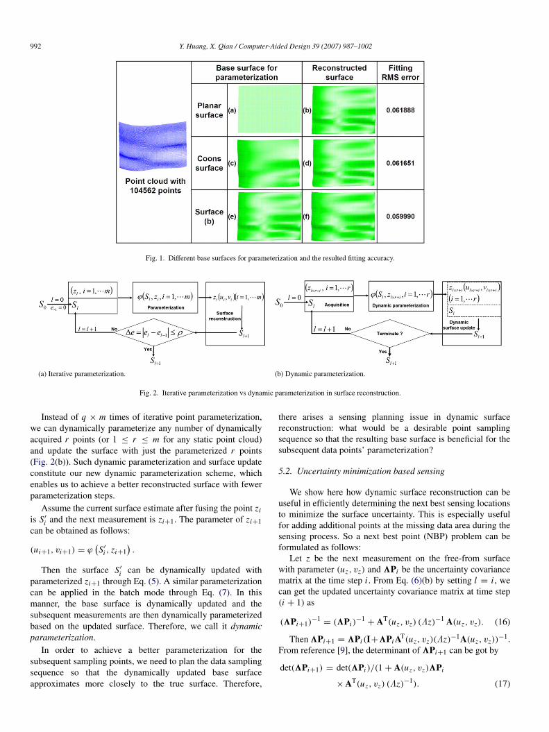
In Fig. 1, we select three kinds of base surfaces to illustratethe effect of data parameterization on surface reconstruction.The first is a planar surface, the second is a Coons surfacedefined by the four boundary curves of the point cloud, andthe last is the surface reconstructed from the point cloud usingthe Kalman filter, in which the data is first parameterized by theplanar surface (Fig. 1(b)). From the fitting accuracy of resultingsurfaces, we can see that the resulting surface has smaller RMSerror when the base surface better approximates the underlyingshape of the point cloud.
Therefore, to achieve a higher accuracy in surfacereconstruction, a better initial base surface for parameterizationis desired. Hence currently an iterative fitting process isoften applied [13,17]. Let z1, z2 · · · zm be the discrete sensedpoints and S0 be initial base surface for parameterization, thiscommon iterative process can be described in Fig. 2(a). In thisiterative parameterization process, the previously reconstructedsurface Sl is used as the base surface for parameterizing theentire point set {zi }. Upon completion, the entire point set isused to reconstruct the surface Sl+1. A termination criterionsuch as the change of root mean squared error ∆e betweenSl+1 and {zi } is used to determine whether such iterationshould continue. As such, the iterative process includes severaltimes of parameterization ϕ (Sl , zi , i = 1, . . . m) and surfacereconstruction that involves the entire point cloud. Assumingq is the times of iterative parameterization and surfacereconstruction, the total number of point parameterization forthe total m measurements is q × m.
992 Y. Huang, X. Qian / Computer-Aided Design 39 (2007) 987–1002
Fig. 1. Different base surfaces for parameterization and the resulted fitting accuracy.
(a) Iterative parameterization. (b) Dynamic parameterization.
Fig. 2. Iterative parameterization vs dynamic parameterization in surface reconstruction.
Instead of q × m times of iterative point parameterization,we can dynamically parameterize any number of dynamicallyacquired r points (or 1 ≤ r ≤ m for any static point cloud)and update the surface with just the parameterized r points(Fig. 2(b)). Such dynamic parameterization and surface updateconstitute our new dynamic parameterization scheme, whichenables us to achieve a better reconstructed surface with fewerparameterization steps.
Assume the current surface estimate after fusing the point ziis S′
i and the next measurement is zi+1. The parameter of zi+1can be obtained as follows:
(ui+1, vi+1) = ϕ(S′
i , zi+1).
Then the surface S′
i can be dynamically updated withparameterized zi+1 through Eq. (5). A similar parameterizationcan be applied in the batch mode through Eq. (7). In thismanner, the base surface is dynamically updated and thesubsequent measurements are then dynamically parameterizedbased on the updated surface. Therefore, we call it dynamicparameterization.
In order to achieve a better parameterization for thesubsequent sampling points, we need to plan the data samplingsequence so that the dynamically updated base surfaceapproximates more closely to the true surface. Therefore,
there arises a sensing planning issue in dynamic surfacereconstruction: what would be a desirable point samplingsequence so that the resulting base surface is beneficial for thesubsequent data points’ parameterization?
5.2. Uncertainty minimization based sensing
We show here how dynamic surface reconstruction can beuseful in efficiently determining the next best sensing locationsto minimize the surface uncertainty. This is especially usefulfor adding additional points at the missing data area during thesensing process. So a next best point (NBP) problem can beformulated as follows:
Let z be the next measurement on the free-from surfacewith parameter (uz, vz) and 3Pi be the uncertainty covariancematrix at the time step i . From Eq. (6)(b) by setting l = i , wecan get the updated uncertainty covariance matrix at time step(i + 1) as
(3Pi+1)−1
= (3Pi )−1
+ AT(uz, vz) (Λz)−1 A(uz, vz). (16)
Then 3Pi+1 = 3Pi (I+3Pi AT(uz, vz)(Λz)−1A(uz, vz))−1.
From reference [9], the determinant of 3Pi+1 can be got by
det(3Pi+1) = det(3Pi )/(1 + A(uz, vz)3Pi
× AT(uz, vz) (Λz)−1). (17)
Y. Huang, X. Qian / Computer-Aided Design 39 (2007) 987–1002 993
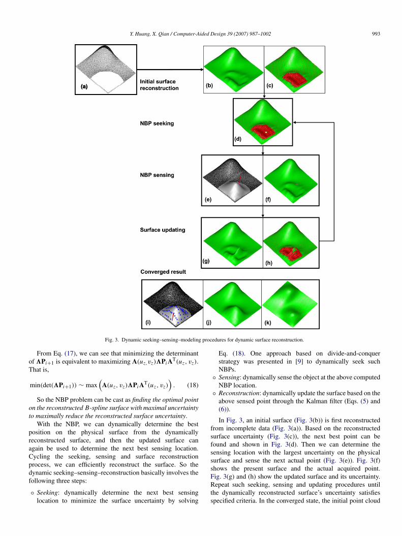
Fig. 3. Dynamic seeking–sensing–modeling procedures for dynamic surface reconstruction.
From Eq. (17), we can see that minimizing the determinantof 3Pi+1 is equivalent to maximizing A(uz,vz)3Pi AT(uz, vz).That is,
min(det(3Pi+1)) ∼ max(
A(uz, vz)3Pi AT(uz, vz))
. (18)
So the NBP problem can be cast as finding the optimal pointon the reconstructed B-spline surface with maximal uncertaintyto maximally reduce the reconstructed surface uncertainty.
With the NBP, we can dynamically determine the bestposition on the physical surface from the dynamicallyreconstructed surface, and then the updated surface canagain be used to determine the next best sensing location.Cycling the seeking, sensing and surface reconstructionprocess, we can efficiently reconstruct the surface. So thedynamic seeking–sensing–reconstruction basically involves thefollowing three steps:
◦ Seeking: dynamically determine the next best sensinglocation to minimize the surface uncertainty by solving
Eq. (18). One approach based on divide-and-conquerstrategy was presented in [9] to dynamically seek suchNBPs.
◦ Sensing: dynamically sense the object at the above computedNBP location.
◦ Reconstruction: dynamically update the surface based on theabove sensed point through the Kalman filter (Eqs. (5) and(6)).
In Fig. 3, an initial surface (Fig. 3(b)) is first reconstructedfrom incomplete data (Fig. 3(a)). Based on the reconstructedsurface uncertainty (Fig. 3(c)), the next best point can befound and shown in Fig. 3(d). Then we can determine thesensing location with the largest uncertainty on the physicalsurface and sense the next actual point (Fig. 3(e)). Fig. 3(f)shows the present surface and the actual acquired point.Fig. 3(g) and (h) show the updated surface and its uncertainty.Repeat such seeking, sensing and updating procedures untilthe dynamically reconstructed surface’s uncertainty satisfiesspecified criteria. In the converged state, the initial point cloud

994 Y. Huang, X. Qian / Computer-Aided Design 39 (2007) 987–1002
and the dynamically acquired points are shown in Fig. 3(i), andthe final surface and its uncertainty are shown in Fig. 3(j) andFig. 3(k).
So here the dynamic surface reconstruction is the key toprovide an updated surface to guide further sensing. It has beenproven that such an uncertainty minimizing process convergesmonotonously [9].
5.3. Low-discrepancy based sensing
In this subsection, we present a low-discrepancy samplingmethod which can take advantage of our dynamic parameteriza-tion to improve the sensing efficiency and reconstruction qual-ity. More specifically, a quasi-Monte Carlo (QMC) method isused to generate the low-discrepancy sensing sequence in theparametric domain.
The discrepancy of sampled points is used to characterizethe quality of the even distribution of discrete points X =
{xi |0 ≤ xi < 1, 1 ≤ i ≤ m} over a given interval (here weassume the interval is [0, 1]). It is defined as
Dm = supJ∈J∗
∣∣∣∣ B(J ; X)
m− |J |
∣∣∣∣ (19)
where J ∗ is the set of intervals [0, t] with 0 < t ≤ 1, B(J ; X)
is the number points in X that fall into the particular interval ofJ , and |J | is the length of the interval J . From Eq. (19), we cansee that
(1) Dm is in between 0 and 1;(2) more evenly distributed points means a smaller value of
Dm . An overly denser or sparser distribution of points in oneparticular interval will lead to a larger value of Dm .
There are several well-known low-discrepancy sequenceconstruction methods such as Faure [3], Halton [7] andNiederreiter [15]. Since the Halton sequence constructionmethod performs well in lower dimensions, in this paper, weselect the Halton construction to successively generate pointswith a low discrepancy. Consider a prime base b, the number ican be written in the form
i = d j b j+ · · · d2b2
+ d1b + d0, 0 ≤ d j < b. (20)
Then the i-th Halton sequence point X i is defined by
X i =d0
b+
d1
b2 + · · · +d j
b j+1 . (21)
In Eq. (21), the i-th Halton sequence point X i is in the openinterval (0, 1).
The 2D Halton point can be composed by using a productof two 1D Halton points with a different base, e.g. b = 2 inthe u direction and b = 3 in the v direction. Since the 2DHalton point is generated in the open interval (0, 1)× (0, 1), nosampling takes place on the surface boundary. Since data pointsnear the vicinities of surface boundary are critical to surfacereconstruction, we introduce an additional one dimensionalquasi-Monte Carlo (QMC) sequence on the boundary of theparametric domain as shown in Fig. 4 (here i starts from 0 inorder to include the four corner points and the base b = 2).
Fig. 4. Sampling scheme for QMC on the boundary of the parametric domain.
Assume we want to obtain r points through QMC. Of thesepoints, [t × r/4] points are sampled on each of the four sidesof the boundary, where t is the percentage of r points to besampled on the boundary (0 ≤ t < 1). Denote the initialbase surface as S0, we can present such a dynamic sampling,sensing and reconstruction strategy through the quasi-MonteCarlo method as follows.Dynamic sampling, sensing, and reconstruction strategyStep 1. Reconstruct the initial surface S from available senseddata points and the a priori surface S0 through the batch fittingmode of the Kalman filter.Step 2. Identify the areas on the parametric domain of thesurface S requiring additional sensing, e.g. missing data areas.(Here we assume the area interval is [u1
∗, u2∗] × [v1
∗, v2∗].)
Step 3. Dynamic sampling, sensing and surface updating.
• Generate [t×r/4] points on each of the four boundary curvesbounding the surface parametric domain with the one-dimensional Halton low-discrepancy sequence constructionmethod (base b = 2).
• Generate the interior r − [t × r/4] × 4 low-discrepancysequence points (ui , vi ), 0 ≤ ui , vi ≤ 1, i = 1, . . . , r − t ∗rand transform {(ui , vi )} into the interval [u∗
1, u∗
2] × [v∗
1 , v∗
2 ]
by ui = u∗
1 + ui ×(u∗
2 − u∗
1)
and vi = v∗
1 + vi × (v∗
2 − v∗
1).• Acquire shape data {zi } on the physical part surface at the
locations closest to {S(ui , vi )} where (ui , vi ) is the sequenceof r points generated above.
• Update the surface S with the acquired point set {zi } throughthe Kalman filter and get the updated surface S′. Set S = S′.
• Repeat the step 3 until a termination criterion is met.For example, a rule of thumb can be that the number ofsensed points should be several times the number of modelparameters.
6. Examples
Four examples are shown below to demonstrate thecapabilities enabled by the dynamic surface reconstruction.
6.1. Example 1: Simulated surface
In Fig. 5, 9 × 10⁴ data points (Fig. 5(b)) are uniformlysampled from a known bi-cubic B-spline surface (28 × 12control points) (Fig. 5(a)). Gaussian noise was added (variance

Y. Huang, X. Qian / Computer-Aided Design 39 (2007) 987–1002 995
(a) A B-spline surface (28 × 12). (b) Uniformly sampled 9 × 10⁴
points from (a).(c) Re-sampled 61127 points from(b).
Fig. 5. Sampled point cloud from a known B-spline surface.
(a) Validate points for RMScomputation (3907 points).
(b) Point-cloud (61,127 points). (c) Initial surface estimateRMS = 8.120393.
(d) The uncertainty of theestimated surface.
(e) Point-cloud + additionalpoints (79 points).
(f) Dynamically reconstructedsurface RMS = 0.067915.
(g) The uncertainty of thereconstructed surface.
Fig. 6. The final surface and its uncertainty through dynamic reconstruction. (For interpretation of the references to colour in this figure legend, the reader is referredto the web version of this article.)
Λzx= Λzy
= Λzz= 0.01). In the noisy data, 61,127 data
points (Fig. 5(c)) are then selected to represent the acquiredpoint cloud and to simulate the measurement with missing dataon the surface.
Since the model structure of the surface is known, a planarsurface with 28 × 12 control points bounding the point cloudis firstly selected as the a priori shape and the unit matrix isdefined as the covariance matrix of its control points. Thenthe points are parameterized with reference to this a priorisurface and the Kalman filter in the batch fitting mode is appliedto estimate the initial surface and its uncertainty. A B-splinesurface is first reconstructed with 28 × 12 control points. Thedynamic seeking, sensing and surface updating is then iteratedto minimize the surface uncertainty as described in Section 5.2.The 79 additional optimal points are added to reduce the surfaceuncertainty. It took total 88.75 s (incremental fitting with theKalman filter: 0.14 s; seeking time: 88.61 s).
In Fig. 6, the initial surface estimate (Fig. 6(c)) and itsuncertainty (the red ellipsoids in Fig. 6(d)) are obtained fromthe point cloud (Fig. 6(b)), and then dynamic seeking, sensingand surface reconstruction is run and 79 accurate points withvariance Λzx
= Λzy= Λzz
= 0.0001 are added to obtain the
surface with lower uncertainty (Fig. 6(f)). We can see that thefinal reconstructed surface has a lower uncertainty (Fig. 6(g))and a smaller RMS error, which is computed with the randomlysampled 3907 points (Fig. 6(a)) in the missing data area at theactual surface.
To validate the sensing efficiency through our dynamicseeking–sensing–reconstruction approach, we compare it witha static plan-reconstruction method and an ad hoc method. Thestatic plan-reconstruction is to pre-plan the optimal points in theparametric domain according to an initial reconstructed surfaceand its static surface uncertainty distribution, and then to mapthem to the physical surface for sensing. This differs from ourdynamic approach in that the parameterization is done with afixed static base surface, which is estimated from the initialpoint cloud (Fig. 6(c)). The ad hoc method refers to a way ofrandomly sensing the points in the missing data areas with astatic base surface for parameterization.
Given an estimated surface and its physical counterpart, anda point’s (u, v) parameter, we can compute the corresponding3D point on the estimated surface and its normal, and thenmapping it onto the physical surface by intersecting the physicalsurface with the ray going through the point and along the
996 Y. Huang, X. Qian / Computer-Aided Design 39 (2007) 987–1002
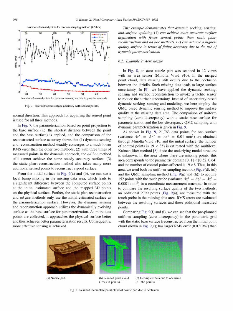
Fig. 7. Reconstructed surface accuracy with sensed points.
normal direction. This approach for acquiring the sensed pointis used for all three methods.
In Fig. 7, the parameterization based on point projection tothe base surface (i.e. the shortest distance between the pointand the base surface) is applied, and the comparison of thereconstructed surface accuracy shows that (1) dynamic sensingand reconstruction method steadily converges to a much lowerRMS error than the other two methods, (2) with three times ofmeasured points in the dynamic approach, the ad hoc methodstill cannot achieve the same steady accuracy surface, (3)the static plan-reconstruction method also takes many moreadditional sensed points to reconstruct a good surface.
From the initial surface in Fig. 6(a) and (b), we can see alocal bump missing in the missing data area, which leads toa significant difference between the computed surface pointsat the initial estimated surface and the mapped 3D pointson the physical surface. Further, the static plan-reconstructionand ad hoc methods only use the initial estimated surface asthe parameterization surface. However, the dynamic sensingand reconstruction approach utilizes the dynamically evolvingsurface as the base surface for parameterization. As more datapoints are collected, it approaches the physical surface betterand thus achieves better parameterization results. Consequently,more effective sensing is achieved.
This example demonstrates that dynamic seeking, sensing,and surface updating (1) can achieve more accurate surfacedigitization with fewer sensed points than static plan-reconstruction and ad hoc methods, (2) can achieve a higher-quality surface in terms of fitting accuracy due to the use ofdynamic parameterization.
6.2. Example 2: Aero nozzle
In Fig. 8, an aero nozzle part was scanned in 12 viewswith an area sensor (Minolta Vivid 910). In the mergedpoint cloud, data missing still occurs due to the occlusionbetween the airfoils. Such missing data leads to large surfaceuncertainty. In [9], we have applied the dynamic seeking,sensing and surface reconstruction to invoke a tactile sensorto reduce the surface uncertainty. Instead of uncertainty-baseddynamic seeking–sensing-and-modeling, we here employ theQMC based dynamic sensing method to improve the surfacequality at the missing data area. The comparison of uniformsampling (zero discrepancy) with a static base surface forparameterization and the low-discrepancy QMC sampling withdynamic parameterization is given in Fig. 9.
As shown in Fig. 9, 21,763 data points for one surface(variance Λzx
= Λzy= Λzz
= 0.01 mm2) are obtainedthrough Minolta Vivid 910, and the initial surface (the numberof control points is 19 × 35) is estimated with the multilevelKalman filter method [8] since the underlying model structureis unknown. In the area where there are missing points, thisarea corresponds to the parametric domain [0, 1] × [0.52, 0.64]
and the number of control points affected is 19×8. Thus, in thisarea, we used both the uniform sampling method (Fig. 9(d), (e))and the QMC sampling method (Fig. 9(g) and (h)) to acquire152 points with the touch probe (variance Λzx
= Λzy= Λzz
=
0.0001 mm2) in a coordinate measurement machine. In orderto compare the resulting surface quality of the two methods,an additional 2799 points (Fig. 9(a)) are measured with thetouch probe in the missing data area. RMS errors are evaluatedbetween the resulting surfaces and these additional measuredpoints.
Comparing Fig. 9(f) and (i), we can see that the pre-planneduniform sampling (zero discrepancy) in the parametric gridwith the static base surface (reconstructed from the initial pointcloud shown in Fig. 9(c)) has larger RMS error (0.071987) than
(a) Nozzle part. (b) Scanned point cloud(185,734 points).
(c) Incomplete data due to occlusion(21,763 points).
Fig. 8. Scanned incomplete point cloud of nozzle part due to occlusion.

Y. Huang, X. Qian / Computer-Aided Design 39 (2007) 987–1002 997
(a) Validation points forRMS computation (2705points).
(b) Point cloud (21,763points).
(c) Initial surface estimateRMS = 0.168823.
(d) Sampling points in theparametric domain (Grid).
(e) Point cloud + additionalgrid points (152 points).
(f) Reconstructed surfaceRMS = 0.071987.
(g) Sampling points in theparametric domain (QMC).
(h) Point cloud + additionalQMC points (152 points).
(i) Dynamicallyreconstructed surfaceRMS = 0.062432.
Fig. 9. Reconstructed surfaces before and after fusing the sensed points.
Fig. 10. The RMS errors vs. the number of additional updating points.
that of the low-discrepancy sequences generated by the QMC(r = 8, t = 0) method with dynamic parameterization (RMSerror 0.062432).
Fig. 10 further compares the RMS error during thesequential process when we add uniform sampled pointswith static parameterization and QMC generated points withdynamic parameterization into the surface reconstruction. Wecan see that dynamic sensing and surface reconstructionthrough quasi-Monte Carlo converges much faster to abetter stable value than the static planned method due tothe combination of low-discrepancy sampling and dynamicparameterization.
6.3. Example 3: Manufactured free-form surface
In Fig. 11, a manufactured surface was scanned with MinoltaVivid910 and 104,562 data points (variance Λzx
= Λzy=
Λzz= 0.01 mm2) were obtained.
In Fig. 12, a planar base surface (the number of the controlpoints P0 : n = 28 × 36 and uncertainty covariance matrix3P0 = I with the dimension 1008 × 1008) is used for
parameterizing the point cloud, and the dynamic sampling andsurface reconstruction described in Section 5.3 with differentnumber of samples each time (r = 2000, t = 0.24;
r = 1000, t = 0.24) are employed to reconstruct the surface.The RMS error between the point cloud and the reconstructedsurface are then calculated. Comparing the resulting surfaces’error with that from the conventional iterative parameterizationmethod shown in Fig. 1, we can see that the dynamicparameterization (both strategies in Fig. 12) can lead to a moreaccurate surface than the iterative parameterization method(Fig. 1(d), RMS = 0.061651 mm) using the Coons surface asthe base surface.
In addition, we also examined the process of dynamicsampling and surface reconstruction.
Fig. 13 gives the comparison of RMS errors between the sur-faces and data points during the process of dynamic parameter-ization and iterative parameterization. In the horizontal axis isthe frequency of sampling r data points. For example 15/30represents 2000 data points have been sampled with QMC for15 times and 1000 data points have been sampled with QMC for30 times. Note, during the dynamic parameterization, differentdata points are sampled from the point set (104,562 points) dueto the use of QMC. Also in Fig. 13 is the iterative parameter-ization shown as a blue dotted line where the entire point set(104,562 points) is parameterized for each iteration.
Fig. 13 shows 20% of data points by the QMC sampling (at10/20) with dynamic parameterization can lead to smaller sur-face fitting RMS error than the parameterizing the entire pointcloud on the static base surface. Dynamically parameterizingthe entire point cloud once with sequences generated by theQMC method (at 52/104) would lead to smaller surface fittingRMS error than iteratively parameterizing the entire point cloudfive times on a static base surface.
This example demonstrates that high quality surface can beobtained much faster by dynamic parameterization of the point

998 Y. Huang, X. Qian / Computer-Aided Design 39 (2007) 987–1002
(a) Measured surface. (b) Scanned point cloud (104,562 points).
Fig. 11. Manufactured surface and scanned point cloud.
Fig. 12. The resulting surface through dynamic sampling and reconstruction (unit: mm).
Fig. 13. RMS errors of the dynamic parameterization and iterativeparameterization. (For interpretation of the references to colour in this figurelegend, the reader is referred to the web version of this article.)
cloud with an appropriate dynamic sampling scheme (QMC inthis paper) than iterative parameterization.
6.4. Example 4: Complex surface reconstruction
In Fig. 14, a human face was scanned by Minolta Vivid910and 27,927 data points (variance Λzx
= Λzy= Λzz
=
0.01 mm2) were obtained.
Fig. 14. A scanned human face and its point cloud.
From the scanned point cloud (Fig. 15(a)), we use a plane(Fig. 15(b)) as the base surface for parameterization and theinitial surface estimate has the number of control points P0 :
40 × 30 and uncertainty covariance matrix 3P0 = I (I isthe unit matrix with the dimension 1200 × 1200). Then thewhole measured points are parameterized to reconstruct thesurface (Fig. 15(c)) using the dynamic sampling and surfacereconstruction strategy as described in Section 5.3 (r =
2000, t = 0.04). Finally we project the boundary curvedefined from the boundary points to the reconstructed surface
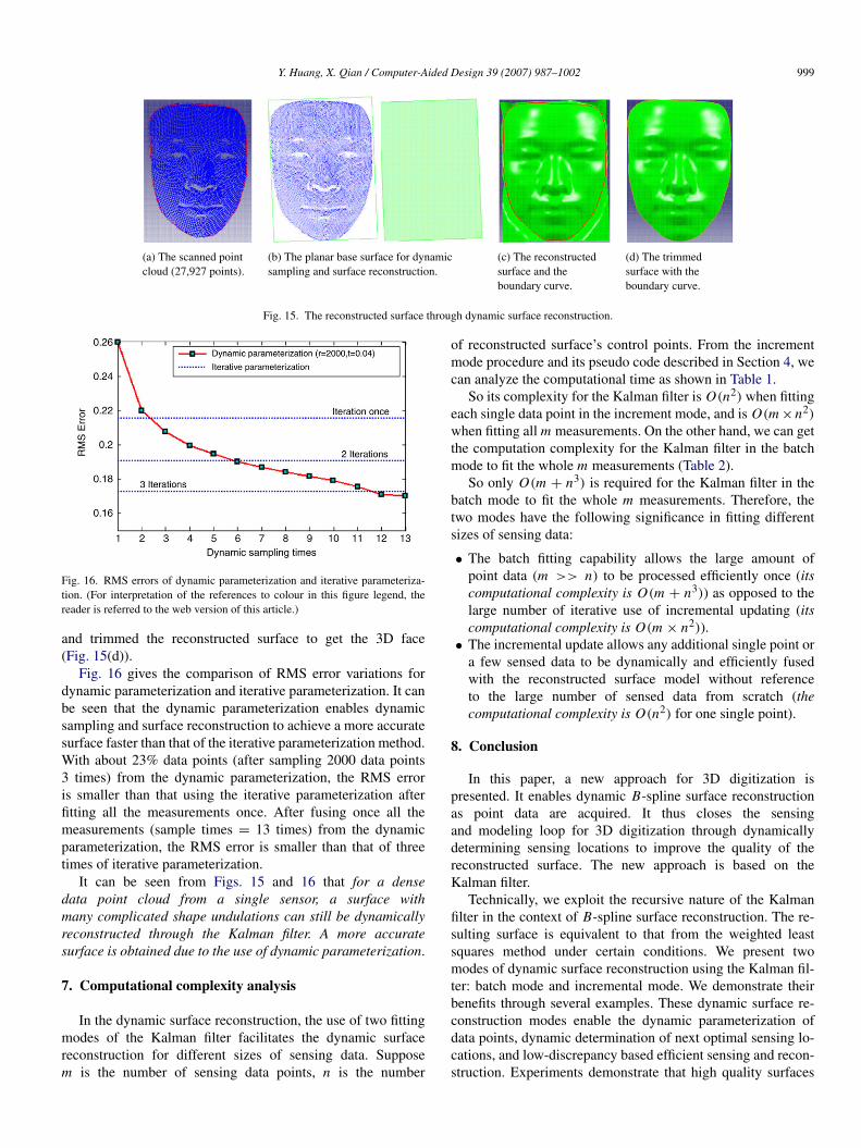
Y. Huang, X. Qian / Computer-Aided Design 39 (2007) 987–1002 999
(a) The scanned pointcloud (27,927 points).
(b) The planar base surface for dynamicsampling and surface reconstruction.
(c) The reconstructedsurface and theboundary curve.
(d) The trimmedsurface with theboundary curve.
Fig. 15. The reconstructed surface through dynamic surface reconstruction.
Fig. 16. RMS errors of dynamic parameterization and iterative parameteriza-tion. (For interpretation of the references to colour in this figure legend, thereader is referred to the web version of this article.)
and trimmed the reconstructed surface to get the 3D face(Fig. 15(d)).
Fig. 16 gives the comparison of RMS error variations fordynamic parameterization and iterative parameterization. It canbe seen that the dynamic parameterization enables dynamicsampling and surface reconstruction to achieve a more accuratesurface faster than that of the iterative parameterization method.With about 23% data points (after sampling 2000 data points3 times) from the dynamic parameterization, the RMS erroris smaller than that using the iterative parameterization afterfitting all the measurements once. After fusing once all themeasurements (sample times = 13 times) from the dynamicparameterization, the RMS error is smaller than that of threetimes of iterative parameterization.
It can be seen from Figs. 15 and 16 that for a densedata point cloud from a single sensor, a surface withmany complicated shape undulations can still be dynamicallyreconstructed through the Kalman filter. A more accuratesurface is obtained due to the use of dynamic parameterization.
7. Computational complexity analysis
In the dynamic surface reconstruction, the use of two fittingmodes of the Kalman filter facilitates the dynamic surfacereconstruction for different sizes of sensing data. Supposem is the number of sensing data points, n is the number
of reconstructed surface’s control points. From the incrementmode procedure and its pseudo code described in Section 4, wecan analyze the computational time as shown in Table 1.
So its complexity for the Kalman filter is O(n2) when fittingeach single data point in the increment mode, and is O(m ×n2)
when fitting all m measurements. On the other hand, we can getthe computation complexity for the Kalman filter in the batchmode to fit the whole m measurements (Table 2).
So only O(m + n3) is required for the Kalman filter in thebatch mode to fit the whole m measurements. Therefore, thetwo modes have the following significance in fitting differentsizes of sensing data:
• The batch fitting capability allows the large amount ofpoint data (m >> n) to be processed efficiently once (itscomputational complexity is O(m + n3)) as opposed to thelarge number of iterative use of incremental updating (itscomputational complexity is O(m × n2)).
• The incremental update allows any additional single point ora few sensed data to be dynamically and efficiently fusedwith the reconstructed surface model without referenceto the large number of sensed data from scratch (thecomputational complexity is O(n2) for one single point).
8. Conclusion
In this paper, a new approach for 3D digitization ispresented. It enables dynamic B-spline surface reconstructionas point data are acquired. It thus closes the sensingand modeling loop for 3D digitization through dynamicallydetermining sensing locations to improve the quality of thereconstructed surface. The new approach is based on theKalman filter.
Technically, we exploit the recursive nature of the Kalmanfilter in the context of B-spline surface reconstruction. The re-sulting surface is equivalent to that from the weighted leastsquares method under certain conditions. We present twomodes of dynamic surface reconstruction using the Kalman fil-ter: batch mode and incremental mode. We demonstrate theirbenefits through several examples. These dynamic surface re-construction modes enable the dynamic parameterization ofdata points, dynamic determination of next optimal sensing lo-cations, and low-discrepancy based efficient sensing and recon-struction. Experiments demonstrate that high quality surfaces

1000 Y. Huang, X. Qian / Computer-Aided Design 39 (2007) 987–1002
Table 1Computational complexity in the incremental mode of the Kalman filter
Computational items Computation complexity
3Pi−1AT(uzi , vzi ) n × 16A(uzi , vzi )3Pi−1AT(uzi , vzi ) n × 16 × 16Ki = 3Pi−1AT(uzi , vzi )(A(uzi , vzi )3Pi−1AT(uzi , vzi ) + Λz)−1 (n × 16 × 16 + 1) + nKi A(uzi , vzi )3Pi−1 [(n × 16 × 16 + 1) + n] + n × n3Pi = 3Pi−1 − Ki A(uzi , vzi )3Pi−1 [(n × 16 × 16 + 1) + n] + n × n + n × nA(uzi , vzi )Pi−1 16Ki (z − A(uzi , vzi )Pi−1) 17 + nPi = Pi−1 + Ki (z − A(uzi , vzi )Pi−1) 17 + n + nPi , 3Pi 2n2
+ 259n + 18
Table 2Computational complexity in the batch mode of the Kalman filter
Computational items Computation complexity∑mi=1 AT(uzi , vzi ) (Λzi )
−1 A(uzi , vzi ) m × 16 × 16(3P0)−1
+∑m
i=1 AT(uzi , vzi ) (Λzi )−1 A(uzi , vzi ) m × 256 + n × n
3Pm =
((3P0)−1
+∑m
i=1 AT(uzi , vzi ) (Λzi )−1 A(uzi , vzi )
)−1m × 256 + n × n + n3∑m
i=1 AT(uzi , vzi ) (Λzi )−1 zi m × 16
Pm = 3Pm((3P0)−1 P0 +
∑mi=1 AT(uzi , vzi ) (Λzi )
−1 zi
)m × 16 + n + n × n
Pm , 3Pm m × 272 + n + 2n2+ n3
can be obtained much faster by dynamic parameterization ofthe point cloud with an appropriate dynamic sampling scheme(e.g. through uncertainty minimization or low-discrepancy se-quences) than iterative parameterization. Further, it does notneed to store the point cloud during the data acquisition processsince all the points are directly incorporated into the surfacemodel during the sensing process.
Future work will aim to extend this dynamic surfacereconstruction to other types of surface representations, aswell as considering non-Gaussian noise in the sensed data.Future work will also study the sensing strategies for dynamicparameterization to optimize the quality of the reconstructedsurface.
Acknowledgements
This work was supported in part by the U.S. NationalScience Foundation Award #0529165 and the Air Force Officeof Scientific Research Award #FA9550-07-1-0241. The authorsalso want to thank Hendrik Speleers for suggesting the quasi-Monte-Carlo method.
Appendix A. Kalman filter for surface reconstruction inthe batch mode
The Kalman filter for the measurements in the batch mode isshown in this appendix.
Lemma 1. Let m be the number of measured pointsz1, z2 . . . zm with uncertainty Λz1,Λz2 . . . ,Λzm , and P0 withuncertainty 3P0 be the set of control points of the initial surfaceestimate, the final surface through the Kalman filter can be
written as
Pm =
((3P0)
−1+
m∑i=1
AT(uzi , vzi )
× (Λzi )−1 A(uzi , vzi )
)−1
×
((3P0)
−1 P0 +
m∑i=1
AT(uzi , vzi ) (Λzi )−1 zi
)(22)
3Pm =
((3P0)
−1+
m∑i=1
AT(uzi , vzi )
× (Λzi )−1 A(uzi , vzi )
)−1
(23)
where A(uzi , vzi ) is B-spline shape function matrix corre-sponding to zi , which is noted as Ai in the following.
Proof. Let K1 be the Kalman gain when fitting the point z1 intothe B-spline surface, and A1 be the B-spline shape functionmatrix corresponding to z1.
The internal state estimate P1 can be got by
P1 = P0 + K1(z1 − A1P0) (24)
and its uncertainty 3P1 = (I − K1A1) 3P0.Eq. (24) can also be written as
P1 = (I − K1A1) P0 + K1z1. (25)
From Eq. (25), we can further infer P2 as
P2 = (I − K2A2) P1 + K2z2
= (I − K2A2) ((I − K1A1) P0 + K1z1) + K2z2

Y. Huang, X. Qian / Computer-Aided Design 39 (2007) 987–1002 1001
= (I − K2A2) (I − K1A1) P0 + (I − K2A2) K1z1 + K2z2
=
2∏i=1
(I − Ki Ai ) P0 +
2∏i=2
(I − Ki Ai ) K1z1 + K2z2 (26)
and its uncertainty 3P2 = (I − K2A2) 3P1 = (I − K2A2)
× (I − K1A1) 3P0 =∏2
i=1 (I − Ki Ai ) 3P0.After all the measurements are fitted, the final state estimate
Pm can be denoted by
Pm =
m∏i=1
(I − Ki Ai ) P0 +
m∏i=2
(I − Ki Ai )
× K1z1 + · · · Km zm (27)
and its uncertainty
3Pm =
m∏i=1
(I − Ki Ai ) 3P0. (28)
For any (1 ≤ r ≤ m), Eq. (28) can be written as
m∏i=r
(I − Ki Ai )
r−1∏i=1
(I − Ki Ai ) 3P0
=
m∏i=r
(I − Ki Ai ) 3Pr−1 = 3Pm . (29)
Multiplying (3Pr−1)−1 to both sides of Eq. (29), we can get
m∏i=r
(I − Ki Ai ) = 3Pm (3Pr−1)−1 . (30)
Substituting Eq. (30) with r = 1, 2, . . . , m into Eq. (27), wecan get the final state estimate Pm as
Pm =
m∏i=1
(I − Ki Ai ) P0
+
m∏i=2
(I − Ki Ai ) K1z1 + · · · + Km zm
= 3Pm (3P0)−1 P0 + 3Pm (3P1)
−1 K1z1
+ · · · + 3Pm (3Pm)−1 Km zm . (31)
From the uncertainty updating equation (Eq. (6)(b)) of theKalman filter, 3Pr (1 ≤ r ≤ m) in Eq. (31) can be got by
(3Pr )−1
= (3Pr−1)−1
+ ATr (Λzr )
−1 Ar . (32)
Multiplying Kr zr to both sides of Eq. (32), we can get
(3Pr )−1 Kr zr =
((3Pr−1)
−1+ AT
r (Λzr )−1 Ar
)3Pr−1AT
r
×
(Λzr + Ar3Pr−1AT
r
)−1zr
=
(AT
r + ATr (Λzr )
−1 Ar3Pr−1ATr
)×
(Λzr + Ar3Pr−1AT
r
)−1zr
= ATr (Λzr )
−1(Λzr + Ar3Pr−1AT
r
)×
(Λzr + Ar3Pr−1AT
r
)−1zr
= ATr (Λzr )
−1 zr . (33)
Substituting Eq. (33) with r = 1, 2, . . . , m into Eq. (31), weget the final state estimate Pm as:
Pm = 3Pm (3P0)−1 P0 + 3PmAT
1 (Λz1)−1 z1
+ · · ·3PmATm (Λzm)−1 zm
= 3Pm
((3P0)
−1 P0 +
m∑i=1
ATi (Λzi )
−1 zi
). (34)
From Eq. (32), we can easily calculate the final stateuncertainty 3Pm by
(3Pm)−1= (3P0)
−1+
m∑i=1
ATi (Λzi )
−1 Ai (35)
or
3Pm =
((3P0)
−1+
m∑i=1
ATi (Λzi )
−1 Ai
)−1
. (36)
Substituting Eq. (36) into Eq. (34), we can get the final stateestimate Pm as
Pm =
((3P0)
−1+
m∑i=1
ATi (Λzi )
−1 Ai
)−1
×
((3P0)
−1 P0 +
m∑i=1
ATi (Λzi )
−1 zi
). (37)
So the lemma is proved. �
Note, there is an assumption in this lemma that themeasurements are first parameterized based on one basesurface.
Appendix B. Weighted least squares for surface recon-struction
The weighted least squares method for surface reconstruc-tion is discussed in this appendix.
The weighted least squares method is often used toreconstruct the surface from the measured points in thestatistical optimal sense. The optimal object function f (P) canbe defined as
Pm = arg minP
(f (P) =
m∑i=1
(zi − Ai P)2
Λzi
). (38)
Differentiating f (P) against P, we can get
∂ f∂P
= −2
(m∑
i=1
ATi (zi − Ai P)
Λzi
)
= −2
(m∑
i=1
ATi (Λzi )
−1 zi −
m∑i=1
ATi (Λzi )
−1 Ai P
). (39)
Let ∂ f∂P = 0, the optimal value Pm can be calculated by
Pm =
(m∑
i=1
ATi (Λzi )
−1 Ai
)−1 m∑i=1
ATi (Λzi )
−1 zi . (40)

1002 Y. Huang, X. Qian / Computer-Aided Design 39 (2007) 987–1002
Eq. (40) can also be written as
Pm
=
[AT1 · · · AT
m](Λz1)−1
. . .
(Λzm)−1
A1
...Am
−1
×[AT
1 · · · ATm](Λz1)−1
. . .
(Λzm)−1
z1
. . .zm
= (ATUA)−1ATUZ (41)
where
A =
A1...
Am
, U =
(Λz1)−1
...
(Λzm)−1
and Z =
z1...
zm
.
From the linear relationship between Pm and Z in Eq. (41), wecan easily get the uncertainty 3Pm as
3Pm = (ATUA)−1ATU3Z((ATUA)−1ATU)T
= (ATUA)−1ATU
Λz1. . .
Λzm
UTA((AT× U × A)−1)T
= (ATUA)−1ATUA(ATUA)−1
= (ATUA)−1
=
[AT1 · · · AT
m](Λz1)−1
. . .
(Λzm)−1
A1
...Am
−1
=
(m∑
i=1AT
i (Λzi )−1Ai
)−1
(42)
References
[1] Allegre R, Chaine R, Akkouche S. Convection-driven dynamic surfacereconstruction. In: Proceedings of shape modeling international. 2005. p.33–42.
[2] Boissonnat JD, Cazals F. Coarse-to-fine surface simplification withgeometric guarantees. Computer Graphics Forum 2001;20(3):490–9.
[3] Bratley P, Fox BL, Niederreiter H. Implementation and tests of low-discrepancy sequences. ACM Transactions on Mathematical Software1992;14:88–100.
[4] Calway A. Recursive estimation of 3D motion and surface structure fromlocal affine flow parameters. IEEE Transactions on Pattern Analysis andMachine Intelligence 2005;27(4):562–74.
[5] Chessa M, Sabatini SP, Solari F, Bisio GM. A recursive approach tothe design of adjustable linear models for complex motion analysis. In:Proceedings of signal processing, pattern recognition, and applications.2007.
[6] Forsey DR, Bartels RH. Surface fitting with hierarchical splines. ACMTransactions on Graphics 1995;22(4):134–61.
[7] Halton JH. On the efficiency of certain quasi-random sequences ofpoints in evaluating multi-dimensional integrals. Journal of NumericMathematics 1960;2:84–90.
[8] Huang Y, Qian X. A stochastic approach to surface reconstruction.In: Proceedings of IDETC/CIE 2006, ASME 2006 international designengineering technical conference & computers and information inengineering conference. 2006.
[9] Huang Y, Qian X. A dynamic sensing-and-modeling approach to3D point- and area-sensor integration. ASME Transactions Journal ofManufacturing Science and Engineering 2007;129(June):623–35.
[10] Kalman RE. A new approach to linear Filtering and prediction problems.Transactions of the ASME Journal of Basic Engineering 1960;82(seriesD):35–45.
[11] Lee S, Wolberg G, Shin SY. Scattered data interpolation with multilevelB-splines. IEEE Transactions on Visualization and Computer Graphics1997;3(3):228–44.
[12] Li YD, Gu PH. Free-form surface inspection techniques state of the artreview. Computer-Aided Design 2004;36(13):1395–417.
[13] Ma W, Kruth JP. Parameterization of randomly measured points for leastsquare fitting of B-spline curves and surfaces. Computer-Aided Design1995;27(9):663–75.
[14] Ma W, He P. B-spline surface local updating with unorganized points.Computer-Aided Design 1998;30(11):853–62.
[15] Niederreiter H. Quasi-Monte Carlo methods and pseudo-randomnumbers. Bulletin of American Mathematical Society 1978;84(6):957–1041.
[16] Phillip NA. Parameterization of clouds of unorganized points usingdynamic base surfaces. Computer-Aided Design 2004;36(7):607–23.
[17] Piegl L, Tiller W. Parameterization for surface fitting in reverseengineering. Computer-Aided Design 2001;33(8):593–603.
[18] Piegl L, Tiller W. The NURBS book. NY: Springer-Verlag; 1997.[19] Rappoport A, Hel-Or Y, Werman M. Interactive design of smooth objects
with probabilistic point constraints. ACM Transactions on Graphics 1994;13(2):156–76.
[20] Szeliski R. Probabilistic modeling of surfaces. Geometric methods incomputer vision, SPIE, vol. 1570. 1991. p. 154–65.
[21] Varady T, Martin R. Reverse engineering handbook of CAGD. NorthHolland; 2002. p. 651–81.
[22] Varady T, Martin RR, Cox J. Reverse engineering of geometric models —an introduction. Computer-Aided Design 1997;29(4):256–68.
[23] Wang YF. A new method for sensor data fusion in machine vision.Geometric methods in computer vision, SPIE, vol. 1570. 1991. p. 31–42.
[24] Wang YF, Wang JF. On 3D model construction by fusing heterogeneoussensor data. CVGIP: Image Understanding 1994;60(2):210–29.
[25] Weiss V, Andor L, Renner G, Varady T. Advanced surface fittingtechniques. Computer Aided Geometric Design 2002;19(1):19–42.
[26] Welch G, Bishop G. An Introduction to the Kalman filter. Technicalreport, TR-95-041. Department of Computer Science, University of NorthCarolina at Chapel Hill; 2004.