Dynamic formation of investment strategies for DC pension plan participants: two new approaches

Vadim Prudnikov

USATU, Ufa, Russia

Radon Workshop on Financial and Actuarial Mathematics for Young Researchers

Linz, Austria, May 30 - 31, 2007

Ufa, Russia

Ufa State Aviation Technical University

The investment in a pension fund

• The investment – is very important field of any pension fund

– for DB plan participants (the actuarial rate)

– for DC plan participants (the pension value, attractiveness for new clients)

• The only relevant characteristic for DC plan participants is the length of the investment horizon

Overview of the problem

• Funds propose to their participants a various number of portfolios

• Two opposite opinions occur regarding the question whether or not investment risk depends on the length of investment horizon

Procedure 1

• Purpose: reproduce the distribution function of the daily logreturns of assets

• Process of the daily logreturns is defined by the following model:

(1)

)1,0(*)2(

)1,0(*)1(

)2(*)2(

)1(*)1(*

*

2

2

NS

NSE

EF

EFSGKS

EXAX

Procedure 2

• Purpose: reproduce the autocorrelation function of the process of the daily logreturns

• According to the signal processing theory:

– to get the power spectrum of the signal

– to go to the gain-frequency characteristic of the signal

– to estimate the parameters of the filter given the gain-frequency characteristic, the order of the filter and the method of estimation

– to pass ‘white’ noise through this filter

First approach, optimization problemt

t

• Consider a participant who has intervals up to retirement, each interval has days long

• Criterion: (2)

• Constrains:(3)

(4)

(5)

- is the minimally allowed proportion of participants’ portfolio invested in each asset

- is the structure of “equal-weighted” portfolio

max)(* txm

0***)()(**)( xVxtAtxVtx TT

ItxD )(

1)(* txI T

TdddD ,...,,

d

TI 1,...,1,1

TMMMx /1,...,/1,/1

t

Estimating of ,• 3 methods for efficiencies calculation, using :

– by direct statistical approach(6)

– by the simulation of the financial market trajectories (using procedure 1 or procedure 2) (7)

- is the value of the quote of asset “i” if the market will go by trajectory “l”

• (8)

(9)

m V

L

llii R

Nm

1,*

1

L

ljljiliji mRmR

Lv

1,, **

1

1,

1,

,,

Ki

lili Q

QMR

1,

,,

li

dtlili Q

QR

kiQ ,

liQM ,

Function A(t), features• - is the number of intervals in the investment horizon of the most

young participants • 2 opinions:

- investment risk of a participant is independent of the length of his investment horizon:

(10)- investment risk of preretired participants must be fewer than it is for young participants

- is a droningly increased function, and

(11)(12)

ttA 1)(

perefT

tA

11A 1perefTA

Function A(t), forms

11

)1*2(*)(

peref

peref

T

TttA

1)1(

)1(

*2)( 2

2t

TtA

peref

1)*21**2()1(

*2)( 2

2 perefperefperef

TtTtT

tA

11

*2

)*2(*sin*)(

peref

peref

T

TttA

otherwise

TttA

peref

,1

2/,1)(

otherwise

TtT

Tt

tA perefperef

peref

,1

2/*23/,1

3/,1

)(

• Linear (13)

• concave (14)

• convex (15)

• S-typed (16)

• 2-stepwised (17)

• 3-stepwised (18)

Second approach

• let to be a minimally allowed step in the change of the portfolio value invested in any particular asset

• to realize the second approach we need:

– to form the countable set of the investment strategies

– to simulate the matrix which contain trajectories of financial market probably motion, for days each

• let S(j,z) be the participants’ portfolio value at the moment of retirement while he applies investment strategy x(j) and financial market moves over trajectory z

• (19)

(20)

PP Ztt *

)(),( tsszjS

tztiPP

ztiPPijxss

ss M

i

,...,1,),1)1(*,(

),*,(*),(*)1(

0,1

)(

1

Second approach, optimization• we treat all the strategies as ‘participants’ of Z independently provided

heats• we transform the matrix of S(j,z) to the matrix of places that the

‘participants’ have achieved, Places(j,z) • we consider as optimal the investment strategy that has the minimal sum of

the places over all the heats: (21)

• 2 opinions– the investment risk of a participant is independent of the length of his

investment horizon, then: optimization is provided at the start time only and the strategies that were once found applies continuously up to retirement

– the investment risk does depend on the participants’ investment horizon, then: optimization is provided in the beginning of every interval

Z

z

zjPlacesj1

* ),(minarg

The mechanism of efficiency checking (1)• group all participants by the length of their investment horizon up to

retirement, accurate within one year

– T is the number of groups we obtained

– the youngest participants has T years or intervals up to retirement

• variant – any approach with specific parameters:

– for the first approach:• the form of A(t)

• the value of

• the method of calculating the efficiencies

– for the second approach:• procedure used to simulate matrix PP

• the option whether the optimization is accomplished periodically or at the start time only

tTTperef

250

*

The mechanism of efficiency checking (2)• input data

– matrix P, containing V trajectories of actual market motion during the period of days. Should be obtained by cutting from actual market trajectories

– parameters of the variants to be checked

• checking of the variants is provided for every group of participants:

– applying the variants of forming strategies over the trajectories of the matrix P

– providing the analysis of the empirical distribution of the value of the portfolio that could be accumulated up to retirement while using one or another variant

KTt peref *

The mechanism of efficiency checking (3)• analysis is provided by means of the stochastic dominance criteria of the

first, the second and the third order for every pair of variants separately

– we consider the variant X as better than variant Y if the following inequality holds:

(22)

(23)

(24)

)(int)(int YspoXspo

T

tt

ttXpXspo1

),()(int

orderunderYiantoveratesdoXiantif

orderunderYiantoveratesdoXiantif

orderunderYiantoveratesdoXiantif

ttgroupforYiantbyateddoisXiantif

ttXp

1varminvar,3

2varminvar,2

3varminvar,1

varminvar,0

),(

Data used for checking

• US financial market indexes (Dow Jones Industrials, index of 13-week US Treasury notes)

• period from 18.09.1986 to 30.04.2007 (5 199 daily quotes for every index)• other parameters were chosen as , , ,so • each trajectory of P must therefore have 40*125+100 = 5 100 daily quotes• the cutting: first trajectory starts 18.09.1986, and every next starts one day

after the preceding (then, V is equal to 5 199 – 5 100 + 1 = 100).

20T 125t 40perefT100K

Approach 1. Experiment 1

Variant 1:

A(t) – linear

Variant 2:

A(t) – concave

Variant 3:

A(t) – convex

Variant 4:

A(t) – S-typed

Variant 5:

A(t) – 2-stepwised

Variant 6:

A(t) – 3-stepwised

0 28 23 24 19 21 115

19 0 22 21 17 17 96

30 29 0 47 6 12 124

16 29 3 0 3 5 56

24 27 34 44 0 11 140

18 32 28 40 6 0 124

Approach 1. Experiment 2

Variant 1:

Variant 2:

Variant 3:

0 4 43 47

43 0 45 88

8 8 0 16

05,0

1,0

025,0

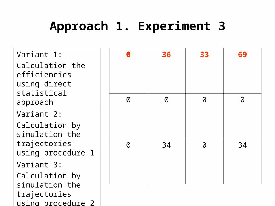
Approach 1. Experiment 3

Variant 1:

Calculation the efficiencies using direct statistical approach

Variant 2:

Calculation by simulation the trajectories using procedure 1

Variant 3:

Calculation by simulation the trajectories using procedure 2

0 36 33 69

0 0 0 0

0 34 0 34

Approach 1. Experiment 4

Variant 1:

A(t) – 2-stepwised

Calculation the efficiencies using direct statistical approach

Variant 2:

A(t) = 1 for all t

1,0

0 49 49

2 0 2

Approach 2. Experiment 5

Variant 1:

Matrix PP is simulated using procedure 1

Variant 2:

Matrix PP is simulated using procedure 2

0 19 19

2 0 2

Approach 2. Experiment 6

Variant 1:

Optimization is provided periodically

Variant 2:

Optimization is provided at the start time only

0 0 0

22 0 22

Experiment 7. Comparison of the approaches

Variant 1:

Approach 1

Variant 2:

Approach 2

Variant 3:

Approach of ‘equal-weighted’ portfolio

0 32 8 40

3 0 0 3

14 23 0 37

Thank you for your attention!