dynamic load balancing - nd.edu

J. Parallel Distrib. Comput. 62 (2002) 1763–1781

A novel dynamic load balancing scheme forparallel systems

Zhiling Lan,a,*,1 Valerie E. Taylor,b,2 and Greg Bryanc,3

aDepartment of Computer Science, Illinois Institute of Technology, Chicago, IL 60616, USAbElectrical and Computer Engineering Department, Northwestern University, Evanston, IL 60208, USA

cNuclear and Astrophysics Laboratory, Oxford University, Oxford OX13RH, UK

Received 23 October 2001; received in revised form 24 June 2002; accepted 10 September 2002

Abstract

Adaptive mesh refinement (AMR) is a type of multiscale algorithm that achieves high

resolution in localized regions of dynamic, multidimensional numerical simulations. One of

the key issues related to AMR is dynamic load balancing (DLB), which allows large-scale

adaptive applications to run efficiently on parallel systems. In this paper, we present an

efficient DLB scheme for structured AMR (SAMR) applications. This scheme interleaves a

grid-splitting technique with direct grid movements (e.g., direct movement from an overloaded

processor to an underloaded processor), for which the objective is to efficiently redistribute

workload among all the processors so as to reduce the parallel execution time. The potential

benefits of our DLB scheme are examined by incorporating our techniques into a SAMR

cosmology application, the ENZO code. Experiments show that by using our scheme, the

parallel execution time can be reduced by up to 57% and the quality of load balancing can be

improved by a factor of six, as compared to the original DLB scheme used in ENZO.

r 2002 Elsevier Science (USA). All rights reserved.

Keywords: Dynamic load balancing; Adaptive mesh refinement; Parallel systems

1. Introduction

Adaptive mesh refinement (AMR) is a type of multiscale algorithm that achieveshigh resolution in localized regions of dynamic, multidimensional numericalsimulations. It shows incredible potential as a means of expanding the tractabilityof a variety of numerical experiments and has been successfully applied to modelmultiscale phenomena in a range of disciplines, such as computational fluiddynamics, computational astrophysics, meteorological simulations, structural

*Corresponding author. Tel.: +312-567-5710; fax: +312-567-5067.

E-mail addresses: [email protected] (Z. Lan), [email protected] (V.E. Taylor), [email protected]

(G. Bryan).1Supported by a grant from the National Computational Science Alliance (ACI-9619019).2Supported in part by NSF NGS grant EIA-9974960 and two NSF ITR grants (ITR-0086044 and ITR-

0085952).3Supported in part by a NASA Hubble Fellowship grant (HF-01104.01-98A).

0743-7315/02/$ - see front matter r 2002 Elsevier Science (USA). All rights reserved.

PII: S 0 7 4 3 - 7 3 1 5 ( 0 2 ) 0 0 0 0 8 - 4

dynamics, etc. The adaptive structure of AMR applications, however, results in loadimbalance among processors on parallel systems. Dynamic load balancing (DLB) isan essential technique to solve this problem. In this paper, we present a novel DLBscheme that integrates a grid-splitting technique with direct grid movements. Weillustrate the advantages of this scheme with a real cosmological application that usesstructured AMR (SAMR) algorithm developed by Berger and Colella [1] in the1980s.

Dynamic load balancing has been intensively studied for more than 10 years and alarge number of schemes have been presented to date [2,5–8,10,12,14,16–18]. Each ofthese schemes can be classified as either Scratch-and-Remap or Diffusion-based

schemes [13]. In Scratch-and-Remap schemes, the workload is repartitioned fromscratch and then remapped to the original partition. Diffusion-based schemes employthe neighboring information to redistribute the load between adjacent processorssuch that global balance is achieved by successive migration of workload fromoverloaded processors to underloaded processors.

With any DLB scheme, the major issues to be addressed are the identification ofoverloaded versus underloaded processors, the amount of data to be redistributedfrom the overloaded processors to the underloaded processors, and the overheadthat the DLB scheme imposes on the application. In investigating DLB schemes, wefirst analyze the requirements imposed by the applications. In particular, wecomplete a detailed analysis of the ENZO application, a parallel implementation ofSAMR in astrophysics and cosmology [3], and identify the unique characteristicsthat impose challenges on DLB schemes. The results of the detailed analysis ofENZO provide four unique adaptive characteristics relating to DLB requirements:(1) coarse granularity, (2) high magnitude of imbalance, (3) different patterns ofimbalance, and (4) high frequency of adaptations. In addition, ENZO employs animplementation that maintains some global information.

The fourth characteristic, the high frequency of adaptations, and the use ofcomplex data structures result in Scratch–Remap schemes being intolerable becauseof the demand to completely modify the data structures without considering theprevious load distribution. In contrast, Diffusion-based schemes are local schemesthat do not utilize the global information provided by ENZO. In [13], it wasdetermined that Scratch-and-Remap schemes are advantageous for problems inwhich high magnitude of imbalance occurs in localized regions, while Diffusion-based schemes generally provide better results for the problems in which imbalanceoccurs globally throughout the computational domain. The third characteristic,different patterns of imbalance, implies that an appropriate DLB scheme shouldprovide good balancing for both situations. Further, the first characteristic, coarsegranularity, is a challenge for a DLB scheme because it limits the quality of loadbalancing. Lastly, ENZO employs a global method to manage the dynamic gridhierarchy, that is, each processor stores a small amount of grid information aboutother processors. This information can be used by a DLB to aid in redistribution.

Utilizing the information obtained from the detailed analysis of ENZO, wedevelop a DLB scheme that integrates a grid-splitting option with direct datamovement. In this scheme, each load-balancing step consists of one or moreiterations of two phases: moving-grid phase and splitting-grid phase. The moving-gridphase utilizes the global information to send grids directly from overloadedprocessors to underloaded processors. The use of direct communication to move thegrids eliminates the variability in time to reach the equal balance and avoids chancesof thrashing [15]. The splitting-grid phase splits a grid into two smaller grids alongthe longest dimension, thereby addressing the first characteristic, coarse granularity.These two phases are interleaved and executed in parallel. For each load-balancing

Z. Lan et al. / J. Parallel Distrib. Comput. 62 (2002) 1763–17811764

step, the moving-grid phase is invoked first; then splitting-grid phase may be invokedif there are no more direct movements. If significant imbalance still exists, anotherround of two phases may be invoked. Further, in order to minimize communica-tional cost of each load balancing step, nonblocking communication is employed inthis scheme and several computation functions are overlapped with thesenonblocking calls.

The efficiency of our DLB scheme on SAMR applications is measured by both theexecution time and the quality of load balancing. In this paper, three metrics areproposed to measure the quality of load balancing. Our experiments show thatintegrating our DLB scheme into ENZO results in significant performanceimprovement for all metrics. For example, the execution time of the AMR64

dataset, a 32� 32� 32 initial grid, on 32 processors is reduced by 57%; and thequality of load balancing is improved by a factor of six.

The remainder of this paper is organized as follows. Section 2 introduces SAMRalgorithm and its parallel implementation, ENZO. Section 3 analyzes the adaptivecharacteristics of SAMR applications. Section 4 describes our dynamic load-balancing scheme. Section 5 presents three load-balancing metrics followed by theexperimental results exploring the impact of our DLB scheme on real SAMRapplications. Section 6 gives a detailed sensitivity analysis of the parameter used inthis proposed DLB scheme. Section 7 describes related work and compares ourscheme with some widely used schemes. Finally, Section 8 summarizes the paper.

2. Overview of SAMR

This section gives an overview of the SAMR method, developed by Berger et al.,and the ENZO code, a parallel implementation of this method for astrophysical andcosmological applications. Additional details about ENZO and the SAMR methodcan be found in [1,3,4,9].

2.1. Layout of grid hierarchy

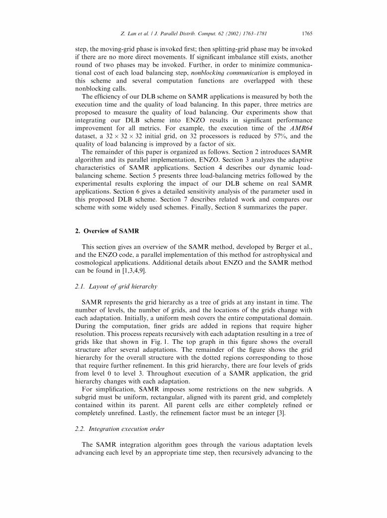
SAMR represents the grid hierarchy as a tree of grids at any instant in time. Thenumber of levels, the number of grids, and the locations of the grids change witheach adaptation. Initially, a uniform mesh covers the entire computational domain.During the computation, finer grids are added in regions that require higherresolution. This process repeats recursively with each adaptation resulting in a tree ofgrids like that shown in Fig. 1. The top graph in this figure shows the overallstructure after several adaptations. The remainder of the figure shows the gridhierarchy for the overall structure with the dotted regions corresponding to thosethat require further refinement. In this grid hierarchy, there are four levels of gridsfrom level 0 to level 3. Throughout execution of a SAMR application, the gridhierarchy changes with each adaptation.

For simplification, SAMR imposes some restrictions on the new subgrids. Asubgrid must be uniform, rectangular, aligned with its parent grid, and completelycontained within its parent. All parent cells are either completely refined orcompletely unrefined. Lastly, the refinement factor must be an integer [3].

2.2. Integration execution order

The SAMR integration algorithm goes through the various adaptation levelsadvancing each level by an appropriate time step, then recursively advancing to the

Z. Lan et al. / J. Parallel Distrib. Comput. 62 (2002) 1763–1781 1765

next finer level at a smaller time step until it reaches the same physical time as that ofthe current level. Fig. 2 illustrates the execution sequence for an application withfour levels and a refinement factor of 2. First, we start with the grids on level 0 withtime step dt: Then the execution continues with the subgrids on level 1, with time stepdt=2:Next, the integration continues with the subgrids on level 2, with time step dt=4;followed by the iteration of the subgrids on level 3 with time step dt=8: When thephysical time at the finest level reaches that at level 0, the grids at level 0 proceed tothe next iteration. The figure illustrates the order in which the subgrids are evolvedwith the integration algorithm.

Fig. 1. SAMR grid hierarchy.

Fig. 2. Integrated execution order (refinement factor ¼ 2).


2.3. ENZO: a parallel implementation of SAMR

Although the SAMR strategy shows incredible potential as a means for simulatingmultiscale phenomena and has been available for over two decades, it is still notwidely used due to the difficulty with implementation. The algorithm is complicatedbecause of the dynamic nature of memory usage, the interactions between differentsubgrids and the algorithm itself. ENZO [3] is one of the successful parallelimplementations of SAMR, which is primarily intended for use in astrophysics andcosmology. It entails solving the coupled equations of gas dynamics, collisionlessdark matter dynamics, self-gravity, and cosmic expansion in three dimensions and athigh spatial resolution. The code is written in C++ with Fortran routines forcomputationally intensive sections and MPI functions for message passing amongprocessors. ENZO was developed as a community code and is currently in use atover six sites.

The ENZO implementation manages the grid hierarchy globally; that is, eachprocessor stores the grid information of all other processors. In order to save spaceand reduce communication time, the notation of ‘‘real’’ grid and ‘‘fake’’ grid is usedfor sharing grid information among processors. Each subgrid in the grid hierarchyresides on one processor and this processor holds the ‘‘real’’ subgrid. All otherprocessors have replicates of this ‘‘real’’ subgrid, called ‘‘fake’’ grids. Usually, the‘‘fake’’ grid contains the information such as dimensional size of the ‘‘real’’ grid andthe processor where the ‘‘real’’ grid resides. The data associated with a ‘‘fake’’ grid issmall (usually a few hundred bytes), while the amount of data associated with a‘‘real’’ grid is large (ranging from several hundred kilobytes to dozens of megabytes).

The current implementation of ENZO uses a simple DLB scheme that utilizes theprevious load information and the global information, but does not address the largegrid sizes (characteristic one). For this original DLB scheme, if the load-balanceratio (defined as MaxLoad/MinLoad) is larger than a hard-coded threshold, the loadbalancing process will be invoked. Here, threshold is used to determine whether aload-balancing process should be invoked after each refinement, and the default isset to 1.50. MaxProc, which has the maximal load, attempts to transfer its portion ofgrids to MinProc, which has the minimal load, under the condition that MaxProc

can find a suitable sized grid for transferring. Here, the suitable size means the size isno more than half of the load difference between MaxProc and MinProc. Fig. 3 givesthe pseudocode of this scheme.

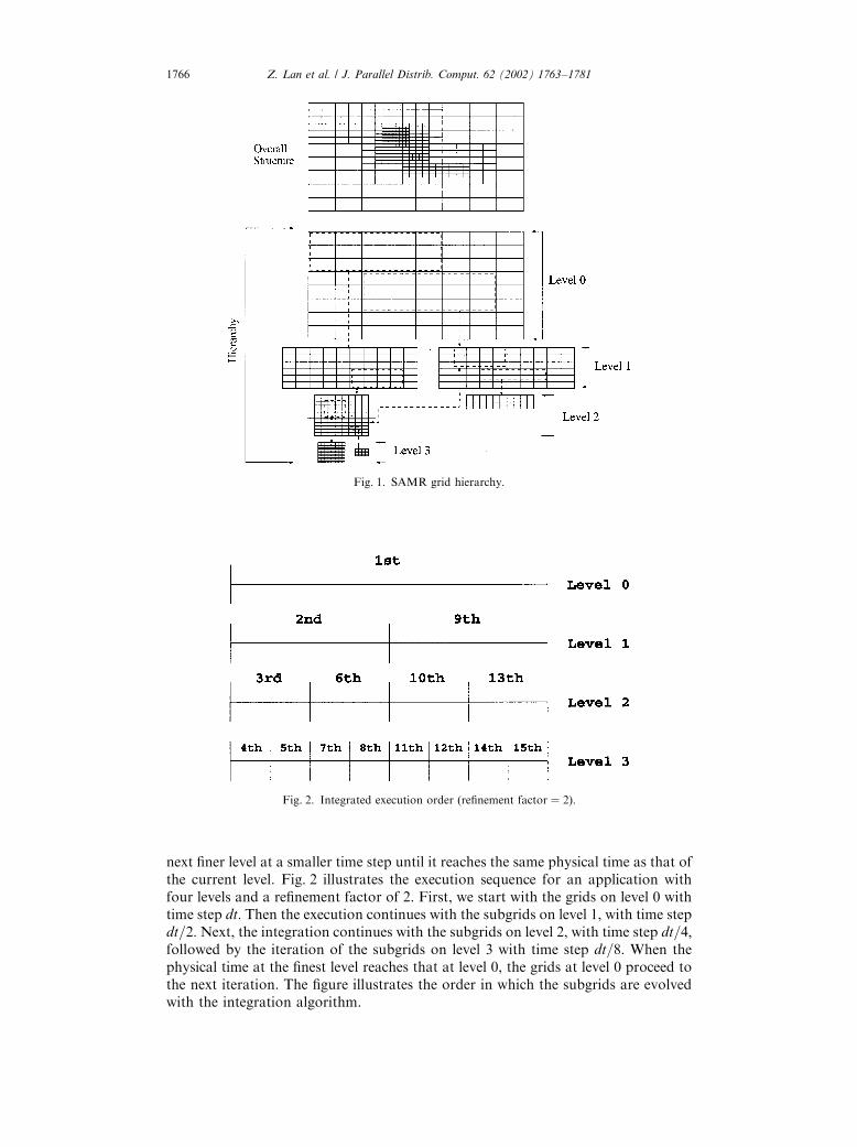
An example of grid movements that occurs with this DLB method is shown inFig. 4. In this example, there are four processors: processor 0 is overloaded with two

Fig. 3. Pseudo-code of the original DLB scheme.


large-sized grids (0 and 1), processor 2 is idle, and processors 1 and 3 areunderloaded. The dash line shows the required load for which all the processorswould have an equal load. After one step of movement with the original DLB, grid 0is moved to processor 2 as shown in Fig. 4. At this point, the original DLB stopsbecause no other grids can be moved. However, as the figure illustrates, the load isnot balanced among the processors. Hence, the original DLB suffers from theproblem of the coarse granularity of the grids. This issue is addressed with our DLBscheme, described in Section 4.

3. Adaptive characteristics of SAMR applications

This section provides some experimental results to illustrate the adaptivecharacteristics of SAMR applications running with ENZO implementation on the250MHz R10000 SGI Origin2000 machine at the National Center for Super-computing Applications (NCSA). Three real datasets (AMR64, AMR128, andShockPool3D) are used in this experiment. Both AMR128 and AMR64 are designedto simulate the formation of a cluster of galaxies; AMR128 is basically a largerversion of AMR64. Both datasets use a hyperbolic (fluid) equation and an elliptic(Poisson’s) equation as well as a set of ordinary differential equations for the particletrajectories. They create many grids randomly distributed across the computationaldomain. ShockPool3D is designed to simulate the movement of a shock wave (i.e., aplane) that is slightly tilted with respect to the edges of the computational domain.This dataset creates an increasing number of grids along the moving shock waveplane. It solves a purely hyperbolic equation. The sizes of these datasets are given inTable 1.

The adaptive characteristics of SAMR applications are analyzed from fouraspects: granularity, magnitude of imbalance, patterns of imbalance, and frequencyof refinements. All the figures shown in this section are obtained by executing ENZOwithout any DLB. This is done to demonstrate the characterization independent ofany DLB.

Coarse granularity: Here, the granularity denotes the size of basic entity for datamovement. For SAMR applications, the basic entity for data movement is a grid.Each grid consists of a computational interior and a ghost zone as shown in Fig. 5.The computational interior is the region of interest that has been refined from theimmediately coarser level; the ghost zone is the part added to exterior ofcomputational interior in order to obtain boundary information. For thecomputational interior, there is a requirement for the minimum number of cells,which is equal to the refinement ratio to the power of the number of dimensions. Forexample, for a 3D problem, if the refinement ratio is 2, then the computationalinterior will have at least 23 ¼ 8 cells. The default size for the ghost zones is set to 3,resulting in each grid having at least ð3þ 2þ 3Þ3 ¼ 512 cells. The grids are often

Fig. 4. An example of load movements using the original DLB scheme.


much larger than this minimum size. Usually, the amount of data associated withgrids varies ranging from 100 KB to 10 MB: Thus the granularity of a typical SAMRapplication is very coarse, thereby making it very hard to achieve a good loadbalance by solely moving these basic entities. Coarse granularity is a challenge for aDLB scheme because it limits the quality of load balancing, thus a desired DLBscheme should address this issue.

High magnitude of imbalance: Fig. 6 shows the load imbalance ratio, defined asmaxðloadÞ=averageðloadÞ; for AMR64 and ShockPool3D, respectively. Here, load isdefined as the total amount of grids in bytes on a processor and the ratio is anaverage over all the adaptations. The ideal case corresponds to the ratio equal to 1.0.The figure indicates that the load imbalance deteriorates as the number of processorsincreases. For AMR64, when the number of processors increases from 4 to 64, theload imbalance ratio increases from 2.02 to 25.64. For AMR128, the results aresimilar to those of AMR64. For ShockPool3D, this ratio increases from 2.19 to 2.96as the number of processors increases from 8 to 64. For both cases, the ratio is

Table 1

Three experimental datasets

Dataset Initial problem size Final problem size Number of adaptations

AMR64 32� 32� 32 4096� 4096� 4096 2500

AMR128 64� 64� 64 8192� 8192� 8192 5000

ShockPool3D 50� 50� 50 6000� 6000� 6000 600

Fig. 5. Components of grids.

Fig. 6. Load imbalance ratio defined as maxðloadÞaverageðloadÞ

� �:


always larger than 2.0, which means a very high magnitude of imbalance exists forboth datasets. Therefore, a DLB scheme is an essential technique for efficientexecution of SAMR applications on parallel systems.

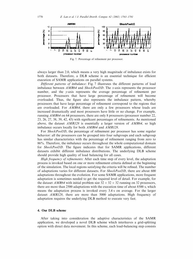
Different patterns of imbalance: Fig. 7 illustrates the different patterns of loadimbalance between AMR64 and ShockPool3D. The x-axis represents the processornumber, and the y-axis represents the average percentage of refinement perprocessor. Processors that have large percentage of refinement will becomeoverloaded. Thus, the figure also represents the imbalance pattern, wherebyprocessors that have large percentage of refinement correspond to the regions thatare overloaded. For AMR64, there are only a few processors whose loads areincreased dramatically and most processors have little or no change. For example,running AMR64 on 64 processors, there are only 8 processors (processor number 22,23, 26, 27, 38, 39, 42, 43) with significant percentages of refinements. As mentionedabove, the dataset AMR128 is essentially a larger version of AMR64, so highimbalance occurs locally for both AMR64 and AMR128.

For ShockPool3D, the percentage of refinement per processor has some regularbehavior: all the processors can be grouped into four subgroups and each subgrouphas similar characteristics with the percentage of refinement ranging from zero to86%. Therefore, the imbalance occurs throughout the whole computational domainfor ShockPool3D. The figure indicates that for SAMR applications, differentdatasets exhibit different imbalance distributions. The underlying DLB schemeshould provide high quality of load balancing for all cases.

High frequency of refinements: After each time step of every level, the adaptationprocess is invoked based on one or more refinement criteria defined at the beginningof the simulation. The local regions satisfying the criteria will be refined. The numberof adaptations varies for different datasets. For ShockPool3D, there are about 600adaptations throughout the evolution. For some SAMR applications, more frequentadaptation is sometimes needed to get the required level of detail. For example, forthe dataset AMR64 with initial problem size 32� 32� 32 running on 32 processors,there are more than 2500 adaptations with the execution time of about 8500 s; whichmeans the adaptation process is invoked every 3:4 s on average. For the largerdataset AMR128, there are more than 5000 adaptations. High frequency ofadaptation requires the underlying DLB method to execute very fast.

4. Our DLB scheme

After taking into consideration the adaptive characteristics of the SAMRapplication, we developed a novel DLB scheme which interleaves a grid-splittingoption with direct data movement. In this scheme, each load-balancing step consists

Fig. 7. Percentage of refinement per processor.


of one or more iterations of two phases: moving-grid phase and splitting-grid phase.The moving-grid phase redistributes grids directly from overloaded processors tounderloaded processors by the guidance of the global information; and the splitting-grid phase splits a grid into two smaller grids along the longest dimension. For eachload-balancing step, the moving-grid phase is invoked first; then splitting-grid phasemay be invoked if no more direct movement can occur. If significant imbalance stillexists, another round of two phases may be invoked. Fig. 8 gives the pseudocode ofour scheme, and the details are given below.

Moving-grid phase: After each adaptation, our DLB scheme is triggered bychecking whether MaxLoad=AvgLoad > threshold : The MaxProc moves its griddirectly to MinProc under the condition that the redistribution of this grid will makethe workload of MinProc reach AvgLoad. Here, AvgLoad denotes the required loadfor which all the processors would have an equal load. Thus, if there is a suitablesized grid, one direct grid movement is enough to balance an underloaded processorby utilizing the global information. This phase continues until either the load-balancing ratio is satisfied or no grid residing on the MaxProc is suitable to bemoved.

Note that this phase differs from the original DLB scheme (Fig. 3) from severalaspects. First, from Fig. 4, it is observed that the original DLB scheme may cause theprevious underloaded processor (processor 2) to be overloaded by solely moving agrid from an overloaded processor to an underloaded processor. Our DLB algorithmovercomes this problem by making sure that any grid movement will make anunderloaded processor reach, but not exceed, the average load.

Fig. 8. Pseudo-code of our DLB scheme.


Second, in this phase, a different metric ðMaxLoad=AvgLoad > thresholdÞ is usedto identify when to invoke load-balancing process in contrast to the metricðMaxLoad=MinLoad > thresholdÞ for the original scheme. The new metric results infewer invocation of load-balancing steps, thereby low overhead. For example,consider two cases with the same average load of 10.0 for a six-processor system: theload distribution is ð20; 8; 8; 8; 8; 8Þ and ð12; 12; 12; 12; 12; 0Þ; respectively. Thedistribution of the second case is preferred over the first case because the maximumrun-time is less. If the threshold is set to 1.50, this moving-grid phase will be invokedfor the first case because MaxLoad

AvgLoad¼ 2:0 is larger than the threshold, while it will not be

invoked for the second case ðMaxLoadAvgLoad

¼ 1:20o1:50Þ: However, the original DLBscheme will invoke grid movements for both cases because the metric ðMaxLoad

MinLoadÞ is

larger than the threshold for both cases, e.g. MaxLoadMinLoad

¼ 2:5 for the first case andMaxLoadMinLoad

¼ N for the second case. Hence, the new metric MaxLoadAvgLoad

> threshold is moreaccurate and results in fewer load-balancing steps.

Splitting-grid phase: If no more direct grid movements can be employed andimbalance still exists, the splitting-grid phase will be invoked. First, the MaxProc

finds the largest grid it owns (denoted as MaxGrid). If the size of MaxGrid is no morethan ðAvgLoad � MinLoadÞ which is the amount of load needed by MinProc, thegrid will be moved directly to MinProc from MaxProc; otherwise, MaxProc splitsthis grid along the longest dimension into two smaller grids. One of the two splitgrids, whose size is about ðAvgLoad � MinLoadÞ; will be redistributed to MinProc.After such a splitting step, MinProc reaches the average load. Note that splittingdoes not mean splitting into equal pieces. Instead, the splitting is done exactly to fillthe ‘‘hole’’ on the MinProc.

After such a splitting phase, if the imbalance still exists, another attempt ofinterleaving moving-grid phase and splitting-grid phase will continue. Eventually,either the load is balanced, which is our goal, or there are not enough grids to beredistributed among all the processors.

To illustrate the use of our DLB scheme, versus the original DLB scheme, we usethe same example given in Fig. 4. In this example, the grid movements of our DLBscheme is shown in Fig. 9. The two grids on overloaded processor 0 are larger thanðthreshold � AvgLoad � MinLoadÞ; so no work can be done in the moving-gridphase and splitting-grid phase begins. First, grid 0 is split into two smaller grids andone of them is transferred to processor 2. This is the first attempt of load balancing.The second attempt of load balancing begins with the direct grid movement of grid 0from processor 0 to processor 1, followed by the grid splitting of grid 1 fromprocessor 0 to processor 3. After two attempts of load balancing, the workload isequally redistributed to all the processors. As we can observe, compared with the

Fig. 9. An example of load movements using our DLB scheme.


grid movements of the original DLB scheme shown in Fig. 4, our DLB schemeinvokes the grid-splitting phase for the case when the direct movement of grids is notenough to handle load imbalance. Our DLB scheme interleaves the grid-splittingtechnique with direct grid movements, thereby improving the load balance.

The use of global load information to move and split the grids eliminates thevariability in time to reach the equal balance and avoids chances of thrashing [15]. Inother words, the situation that multiple overloaded processors send their workloadto an underloaded processor and make it overloaded will not occur by using theproposed DLB. Note that both the moving-grid phase and splitting-grid phaseexecute in parallel. For example, suppose there are eight processors as shown inFig. 10. If the MaxProc and MinProc are processors 0 and 5, respectively, all theprocessors know which grid will be moved/split from processor 0 to processor 5 bythe guidance of the global information. Then processor 0 moves/splits its grid (i.e.the ‘‘real’’ grid) to processor 5. In parallel, other processors first update their view ofload distribution of this grid movement from processor 0 to processor 5, thencontinue load-balancing process. If the new MaxProc and MinProc are processor 1and 2 respectively, then processor 1 will move/split its grid (i.e. ‘‘real’’ grid) toprocessor 2, and this process will be overlapped with the movement from processor 0to processor 5. The remaining processors (3, 4, 6 and 7) continue with first updatingtheir view of load distribution of the grid movement from processor 1 to processor 2followed by calculating the next MaxProc and MinProc. Because the new MaxProc

and MinProc are processor 0 and 3, respectively, so processor 3 has to wait forprocessor 0 which is still in the process of transferring its workload to processor 5.

In order to minimize the overhead of the scheme, nonblocking communication isexplored in this scheme. In the mode of nonblocking communication, a nonblockingpost-send initiates a send operation and returns before the message is copied out ofthe send buffer. A separate complete-send call is needed to complete thecommunication. The nonblocking receive is proceeded similarly. In this manner,the transfer of data may proceed concurrently with computations done at both thesender and the receiver sides. In the splitting-grid phase, nonblocking calls areexplored and being overlapped with several computation functions.

Fig. 10. An illustration of the parallelism in our DLB scheme.


5. Experimental results

The potential benefits of our DLB scheme were examined by executing real SAMRapplications running ENZO on parallel systems. All the experiments were executedon the 250 MHz R10000 SGI Origin2000 machines at NCSA. The code wasinstrumented with performance counters and timers, which do not require any I/O atrun-time. The threshold is set to 1.20.

5.1. Comparison metrics

The effectiveness of our DLB scheme is measured by both the execution time andthe quality of load balancing. In this paper, three metrics are proposed to measurethe quality of load balancing. Note that each metric below is arithmetic average overall the adaptations.

Imbalance ratio is defined as

imbalance ratio ¼

PNj¼1

MaxLoadðjÞAvgLoadðjÞ

N; ð1Þ

where N is number of adaptations, MaxLoadðjÞ denotes the maximal amount of loadof a processor for the jth adaptation, and AvgLoadðjÞ denotes the average load of allthe processors for the jth adaptation. It is clear that imbalance ratio is greater orequal to 1.0. The closer it is to 1.0 the better; the value of 1.0 implies equal loaddistribution among all processors.

Standard deviation of imbalance ratio is defined as

avg std ¼

PNj¼1

ffiffiffiffiffiffiffiffiffiffiffiffiffiffiffiffiffiffiffiffiffiffiffiffiffiffiffiffiffiffiffiffiffiffiffiffiffiffiffiffiffiffiffiffiffiffiffiffiffiffiffiPP

i¼1ðMaxLoadðjÞ

LiðjÞ�

MaxLoadðjÞAvgLoadðjÞ Þ

2

P�1

r

N; ð2Þ

where P is number of processors and LiðjÞ denotes the workload of ith processor forthe jth adaptation. By definition, the capacity to keep avg std low during theexecution is one of the main quality metrics for an efficient DLB. The capacity tohave avg std be a small fraction of imbalance ratio indicates that imbalance ratio cantruly represent the imbalance over all the adaptations.

Percentage of idle processors is defined as

idle procs ¼

PNj¼1 idleðjÞ

N; ð3Þ

where idleðjÞ is the percentage of idle processors for the jth adaptation. Here, an idleprocessor is the processor whose amount of load is zero. As mentioned above, due tothe coarse granularity and the minimal size requirement of SAMR applications, it ispossible that there may be some idle processors for each iteration. Obviously, thesmaller this metric, the better the load is balanced among the processors.

5.2. Execution time

Fig. 11 compares the total execution times with varying numbers of processors bycomparing our DLB scheme with the original DLB scheme for the datasets AMR64,AMR128, and ShockPool3D. Table 2 summarizes the relative improvements byusing our DLB scheme. It is observed that our DLB scheme greatly reduces theexecution time, especially when the number of processors is more than 16. Therelative improvements of execution time are as follows: between 12.60% and 57.54%for AMR64, between �4:84% and 20.17% for AMR128, and between 8.07% and


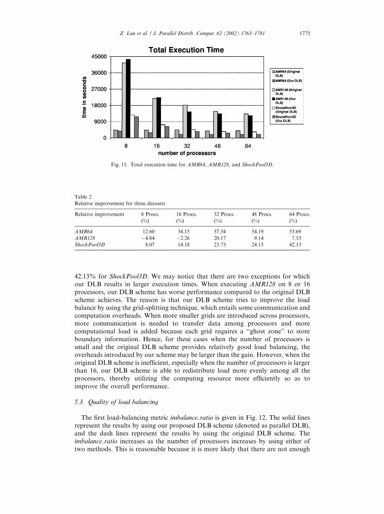
42.13% for ShockPool3D. We may notice that there are two exceptions for whichour DLB results in larger execution times. When executing AMR128 on 8 or 16processors, our DLB scheme has worse performance compared to the original DLBscheme achieves. The reason is that our DLB scheme tries to improve the loadbalance by using the grid-splitting technique, which entails some communication andcomputation overheads. When more smaller grids are introduced across processors,more communication is needed to transfer data among processors and morecomputational load is added because each grid requires a ‘‘ghost zone’’ to storeboundary information. Hence, for these cases when the number of processors issmall and the original DLB scheme provides relatively good load balancing, theoverheads introduced by our scheme may be larger than the gain. However, when theoriginal DLB scheme is inefficient, especially when the number of processors is largerthan 16, our DLB scheme is able to redistribute load more evenly among all theprocessors, thereby utilizing the computing resource more efficiently so as toimprove the overall performance.

5.3. Quality of load balancing

The first load-balancing metric imbalance ratio is given in Fig. 12. The solid linesrepresent the results by using our proposed DLB scheme (denoted as parallel DLB),and the dash lines represent the results by using the original DLB scheme. Theimbalance ratio increases as the number of processors increases by using either oftwo methods. This is reasonable because it is more likely that there are not enough

Fig. 11. Total execution time for AMR64, AMR128, and ShockPool3D.

Table 2

Relative improvement for three datasets

Relative improvement 8 Procs. 16 Procs. 32 Procs. 48 Procs. 64 Procs.

ð%Þ ð%Þ ð%Þ ð%Þ ð%Þ

AMR64 12.60 34.15 57.54 54.19 53.69

AMR128 �4.84 �2.26 20.17 9.14 7.53

ShockPool3D 8.07 14.18 23.73 24.15 42.13


grids to be redistributed among processors if there are more processors. Ourproposed DLB, however, is able to significantly reduce the imbalance ratio byinterleaving direct grid movement with grid splitting for all cases. Further, theamount of improvement gets larger as the number of processors increases. Ingeneral, the imbalance ratio by using our DLB scheme is always less than 1.80, whichis significant. As compared to the original DLB scheme, the relative improvement ofimbalance ratio is in the range of 33%–615% by using our DLB scheme. The resultof the second load-balancing metric, avg std (not shown), indicates that the standarddeviation of imbalance ratio is quite low (less than 0.035), which means thatimbalance ratio can truly represent the load imbalance among all processors.

The third metric percentage of idle processors is shown in Fig. 13. The solid linesand the dash lines represent results by using our DLB (denoted as parallel DLB) andthe original DLB scheme respectively. The results indicate that the metric increasesas the number of processors increases for both schemes. This is due to the fact that itis more likely there are not enough grids for movement when there are moreprocessors. However, the percentage of idle processors is much lower by using ourDLB scheme; the metric ranges from zero to approximately 25% for our DLBscheme, as compared to 5.9%–81.2% for the original DLB scheme. Largerpercentage of idle processors means more computing resources are wasted.

Fig. 13. Average percentage of idle processors.

Fig. 12. Imbalance ratio for three datasets.


6. Sensitivity analysis

A parameter called threshold is used in our DLB scheme (see Fig. 8), whichdetermines whether a load-balancing process should be invoked after eachrefinement. Intuitively, the ideal value should be 1.0, which means all the processorsare evenly and equally balanced. However, the closer this threshold is to 1.0, themore load-balancing actions are entailed, so the more overhead may be introduced.Furthermore, for SAMR applications, the basic entity is a ‘‘grid’’ which has aminimal size requirement. Thus the ideal situation in which the load is perfectlybalanced may not be obtained. The threshold is used to adjust the quality of loadbalancing, whose value influences the efficiency of the overall DLB scheme. What isthe optimal value for this threshold is the topic of this section. We give theexperimental results to compare the performance and the quality of load balancingby varying threshold from a small value of 1.10 to a large value of 2.00 and identifythe optimal value for the parameter.

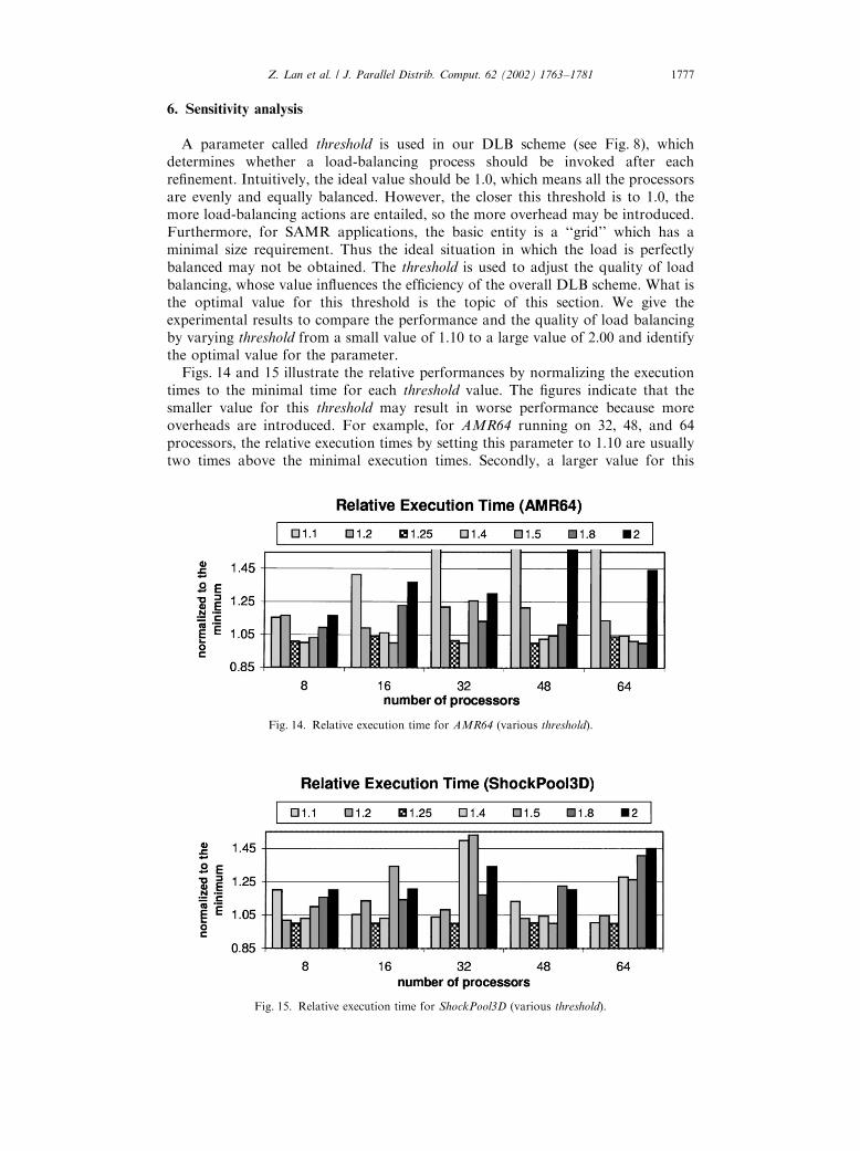
Figs. 14 and 15 illustrate the relative performances by normalizing the executiontimes to the minimal time for each threshold value. The figures indicate that thesmaller value for this threshold may result in worse performance because moreoverheads are introduced. For example, for AMR64 running on 32, 48, and 64processors, the relative execution times by setting this parameter to 1.10 are usuallytwo times above the minimal execution times. Secondly, a larger value for this

Fig. 14. Relative execution time for AMR64 (various threshold).

Fig. 15. Relative execution time for ShockPool3D (various threshold).


threshold may also result in a worse performance due to the poorer quality of loadbalancing. For example, for ShockPool3D, by setting this parameter to 2.00, therelative execution times are 20–45% above the minimal execution times. Both figuresindicate that setting threshold to 1.25 results in the best performance in terms ofexecution time because the relative execution times are always no more than 5%above the minimal execution times.

Figs. 16 and 17 illustrate the quality of load balancing with varying values ofthreshold for AMR64 and ShockPool3D. Here, the quality of load balancing ismeasured by the imbalance ratio: From both figures, it is clear that the smaller is thethreshold, the smaller is the imbalance ratio; thereby resulting in a higher quality ofload balancing. A smaller value of threshold indicates that more load-balancingactions may be entailed to balance the workload among the processors. Further, wecan observe that imbalance ratio gets larger as the number of processors increases.When the number of processors is increased, there may not be enough grids to bedistributed among the processors, which results in lower quality of load balancing. Itseems that the best case is to set threshold to a smaller value, such as 1.10. However,this small value means more load-balancing attempts are invoked, which wouldintroduce more overhead and the overall performance may be deteriorated as shownin Figs. 14 and 15. For both datasets, our results of idle procs (not shown) indicate

Fig. 16. Quality of load balancing for AMR64 (various threshold).

Fig. 17. Quality of load balancing for ShockPool3D (various threshold).


that there is no significant difference of its values with the varying values ofthreshold.

By combining the results in Figs. 14–17, we determine that setting threshold to bearound 1.25 would result in the best performance in terms of execution time, as wellas the acceptable quality of load balancing.

7. Related work

Our DLB scheme is not a Scratch–Remap scheme because it takes intoconsideration the previous load distribution during the current redistributionprocess. As compared to Diffusion-based scheme, our DLB scheme differs from it intwo manners. First, our DLB scheme addresses the issue of coarse granularity ofSAMR applications. It splits large-sized grids located on overloaded processors ifjust the movement of grids is not enough to handle load imbalance. Second, ourDLB scheme employs the direct data movement between overloaded and under-loaded processors by the guidance of global load information.

Grid splitting is a well-known technique and has been applied in severalresearch works. Rantakokko uses this technique in his static load-balancingscheme [11] which is based on recursive spectral bisection. The main purpose ofusing grid splitting is to reuse a solver for a rectangular domain. In our scheme,the grid-splitting technique is combined with direct grid movements to providean efficient dynamic load balancing scheme. Here, grid splitting is used toreduce the granularity of data moved from overloaded to underloadedprocessors, thereby resulting in equalizing load throughout execution of the SAMRapplication.

8. Summary

In this paper, we presented a novel dynamic load-balancing scheme forSAMR applications. Each load-balancing step of this scheme consists of twophases: moving-grid phase and splitting-grid phase. The potential benefits of ourscheme were examined by incorporating our DLB scheme into a real SAMRapplication, ENZO. The experiments show that our scheme can significantlyimprove the quality of load balancing and reduce the total execution time, ascompared to the original DLB scheme. By using our DLB scheme, the totalexecution time of SAMR applications was reduced up to 57%, and the quality ofload balancing was improved significantly especially when the number of processorsis larger than 16.

While the focus of this paper is on SAMR, some techniques can be easily extendedto other applications, such as using grid splitting to address coarse granularity ofbasic entity, utilizing some global load information for data redistribution,interleaving direct data movements with splitting technique, and the imbalancedetection by using maxðloadÞ=averageðloadÞ to measure load imbalance. Further, webelieve the techniques are not limited to SAMR applications and should havebroader applicability, such as unstructured AMR. For example, it could be extendedto any application with the following characteristics: (1) it has coarse granularity and(2) each processor has a global view of load distribution, that is, each processorshould be aware of the load distribution of other processors.


Acknowledgments

The authors thank Michael Norman at UCSD for numerous comments andsuggestions that contributed to this work. We also acknowledge the National Centerfor Supercomputing Application (NCSA) for the use of the SGI Origin machines.

References

[1] M. Berger, P. Colella, Local adaptive mesh refinement for shock hydrodynamics, J. Comput. Phys. 82

(1) (May 1989) 64–84.

[2] E. Boman, K. Devine, B. Hendrickson, W. Mitchell, M. John, C. Vaughan, Zoltan: a dynamic load-

balancing library for parallel applications, World Wide Web, http://www.snl.gov/zoltan.

[3] G. Bryan, Fluid in the universe: adaptive mesh refinement in cosmology, Comput. Sci. Eng. 1 (2)

(March/April 1999) 46–53.

[4] G. Bryan, T. Abel, M. Norman, Achieving extreme resolution in numerical cosmology using adaptive

mesh refinement: resolving primordial star formation, in: Proceedings of SC2001, Denver, CO, 2001.

[5] G. Cybenko, Dynamic load balancing for distributed memory multiprocessors, IEEE Trans. Parallel

Distrib. Systems 7 (October 1989) 279–301.

[6] K. Dragon, J. Gustafson, A low-cost hypercube load balance algorithm, in: Proceedings of the

Fourth Conference on Hypercubes, Concurrent Computations and Applications, 1989, pp. 583–590.

[7] G. Horton, A multilevel diffusion method for dynamic load balancing, Parallel Comput. (19) (1993)

209–218.

[8] F. Lin, R. Keller, The gradient model load balancing methods, IEEE Trans. Software Eng. 13 (1)

(January 1987) 8–12.

[9] M. Norman, G. Bryan, Cosmological adaptive mesh refinement, Comput. Astrophys. (1998).

[10] L. Oliker, R. Biswas, Plum: parallel load balancing for adaptive refined meshes, J. Parallel Distrib.

Comput. 47 (2) (1997) 109–124.

[11] J. Rantakokko, A framework for partitioning domains with inhomogeneous workload, Technical

Report, Uppsala University, Sweden, 1997.

[12] K. Schloegel, G. Karypis, V. Kumar, Multilevel diffusion schemes for repartitioning of adaptive

meshes, J. Parallel Distrib. Comput. 47 (2) (1997) 109–124.

[13] K. Schloegel, G. Karypis, V. Kumar, A performance study of diffusive vs. remapped load-balancing

schemes, in: Proceedings of the 11th International Conference on Parallel and Distributed

Computing, 1998.

[14] A. Sohn, H. Simon, Jove: a dynamic load balancing framework for adaptive computations on an sp-2

distributed multiprocessor, NJIT CIS Technical Report, New Jersey, 1994.

[15] F. Stangenberg, Recognizing and avoiding thrashing in dynamic load balancing, Technical Report,

EPCC-SS94-04, September 1994.

[16] KeLP Team, The KeLP programming system, World Wide Web, http://www-cse.ucsd.edu/groups/

hpcl/scg/kelp.html, 1999.

[17] C. Walshaw, Jostle: partitioning of unstructured meshes for massively parallel machines, in:

Proceedings of Parallel CFD’94, 1994.

[18] M. Willebeek-LeMair, A. Reeves, Strategies for dynamic load balancing on highly parallel

computers, IEEE Trans. Parallel Distrib. Systems 4 (9) (September 1993) 979–993.

Zhiling Lan received her BS in mathematics from Beijing Normal University and her MS in

applied mathematics from Chinese Academy of Sciences in 1992 and 1995, respectively; she

received her Ph.D. in computer engineering from Northwestern University in 2002. She is

currently a faculty member in the Department of Computer Science at Illinois Institute of

Technology starting from August 2002. Her research interests are in the area of parallel and

distributed systems, and performance analysis and modeling. She is a member of IEEE and

ACM.

Valerie E. Taylor is a professor in the Electrical and Computer Engineering Department at

Northwestern University, where she leads the CELERO Performance Analysis Research

Group. She received her B.S. in computer and electrical engineering and M.S. in electrical

engineering from Purdue University in 1985 and 1986, respectively; she received her Ph.D. in


http://www.snl.gov/zoltan

http://www-cse.ucsd.edu/groups/hpcl/scg/kelp.html

http://www-cse.ucsd.edu/groups/hpcl/scg/kelp.html

electrical engineering and computer science from University of California at Berkeley in 1991.

Valerie Taylor holds an US patent for her dissertation work on sparse matrices. She received a

National Science Foundation National Young Investigator Award in 1993. Her research

interests are in the area of high performance computing, with particular emphasis on

performance analysis of parallel and distributed scientific applications. She has published over

70 papers in the area of high performance computing. Currently, she is a member of ACM and

a senior member of IEEE.

Greg Bryan received a B.Sc. from the University of Calgary in 1991 and a Ph.D. in

astrophysics from the University of Illinois in 1996. He is currently a faculty member in the

Department of Physics at Oxford University and performs research both in formation of

structure in the universe, and in the development of computational techniques for modeling

the formation and evolution of multi-scale systems.


dynamic load balancing - nd.edu

Documents