Portland, Oregon

NOISE-CON 2011 2011 July 25-27

Dynamic measurements of wind turbine acoustic signals, employing sound quality engineering methods considering the time and frequency sensitivities of human perception Wade Bray1)

HEAD acoustics, Inc. 6964 Kensington Road Brighton, MI 48116 Richard James2)

E-Coustic Solutions Okemos, MI 48805 A set of binaural time-recordings and analyses of wind turbine noise outside and inside a residence in Huron County, Michigan, made over two days and the intervening night in December 2009, is presented, centering on analysis at the time/frequency resolutions of human hearing according to the well-established practices of sound quality engineering and Soundscaping [1]. The purpose of this paper is to present wind turbine acoustic measurements at these time-frequency scalings and to suggest that such consideration, frequently neglected in favor of frequency resolution and long-term level averages, could augment the perceptually inappropriate averages (often A-weighted) typically taken over much longer intervals. The authors maintain that most measurements of wind turbines up to now have not considered, or not adequately considered, these signals’ very complex and varying behaviors at the time/bandwidth scalings of human perception. Although treating wind turbine noise aspects at all relevant frequencies, this paper will concentrate on low-frequency information.

1. INTRODUCTION Human hearing and other senses (vision, touch…) are sensitive to and provide information from our environment on a micro-time scale. We emit information in spoken communication on a micro-time scale. Many acoustical measurements (Leq, etc.) are on a macro-time scale, yet we are immersed over macro-time in a life comprised of micro-time detail. It is incorrect to present only macro-time measurement results as representative of sensation, and perhaps impossible to try to combine both scales in a macro-time-only context (this paper will suggest some ways), but we must always try to assemble context-valid measurement data sets best representing “the human function.” The scientific fields of sound quality engineering and Soundscaping provide insights in how this dichotomy or polychotomy might be approached. "Conventional methods often reduce the complexity of reality into controllable variables, which supposedly represent the 1) Email address: wbray@headacoustics.com 2) Email address: rickjames@e-coustic.com

scrutinized object – 'impoverished dimensionality'” (Schulte-Fortkamp and Bray, SAE Sound Quality Workshop 2009). Low-frequency noise, particularly time-structured and even at low levels, is a current “hot topic in acoustics” in the Acoustical Society of America [2], and has unusual annoyance properties related to other frequency content or its absence. Situations of isolated low-frequency noise without other noise or with other noise of very low level may be more annoying than when other noise is present with overall level or loudness consequently higher [3]. A common measurement with wind turbines employs very high frequency-domain resolution enabling display of the harmonic series due to the blade-pass rate as an apparent near-steady pure tone family (macro-time scale), yet in the micro-time sensation range of human hearing and the function of its transducer, that result is completely unconnected to the high crest factor short-term events at low and very low frequencies resolvable at shorter time-scales and by wider acquisition bandwidths. The central measurement guiding other supporting analyses in any class of sound quality/human perception issues must be an auditorily-relevant one, involving the time-scale of the human receiver. At low frequencies, time and frequency resolutions become strenuously at odds with each other and challenge measurement. Once “the human receiver is served,” other resolutions and measures may be employed to investigate causes. The properties of human hearing cause the sensation of any audible sound below about 50 Hz, even a continuous sine, to be perceived as time-varying, with the sensation of periodic time structure increasing with decreasing signal frequency. This pure-tone finding (to be discussed) has been investigated beginning in 2010 and involves listening tests covering, as yet, a small number of test subjects [4, 5, 6]. More research needs to be done.

2. DESCRIPTION OF TEST SITE; LOCAL CONDITIONS

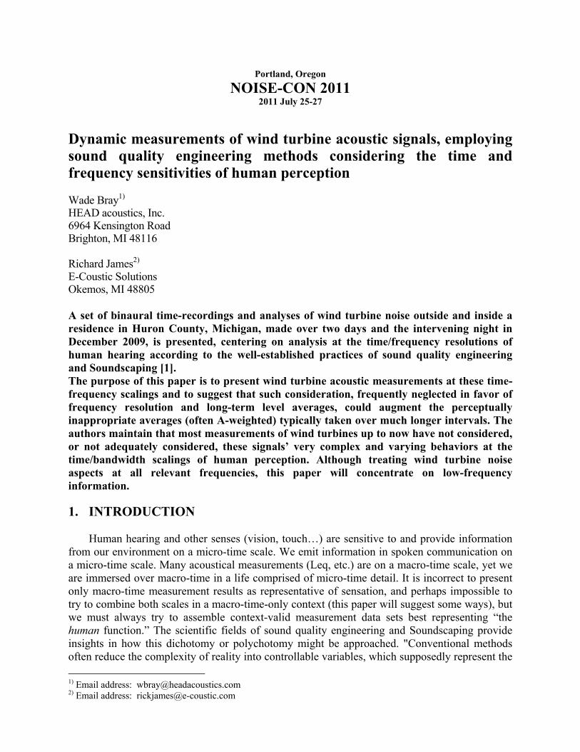
This wind turbine noise field test was conducted on December 17 and 18, 2009. The test location was outside a residence in Ubly, Michigan. The wind turbine utility which operates the wind turbines in this community is Michigan Wind I, which is comprised of 46 GE 1.5-MW SLE wind turbines. The facility began commercial operation in mid-December of 2008. Figure 1 shows the location of the residence in the upper left quadrant and the wind turbine closest to this residence in the lower right quadrant. The distance between the test site and the base of the wind turbine is approximately 1500 feet. The trees and shrubs between the test site and turbine base visually obscured the base of the turbine.

Figure 1 - Overview of Field Test Location, Michigan Wind I. The wind turbine which dominated the sound field during the test as it appears from the road and driveway of the residence is shown in lower right quadrant of Figure 1.

2.1 Weather Wind speed was under 10 mph from the start of the test on the afternoon of December 17, 2009 through noon of the following day. Wind direction was from the southeast during the test period. Temperatures ranged from 17 to 26 degrees F. with a mean of 22. Relative humidity ranged from 64 to 86%. No precipitation occurred during the test period. Skies were generally overcast with no extended cloudless periods. 2.2 Instrumentation The field data were obtained and analyzed as follows:

1) Binaural Artificial HEAD Measurement System (HEAD acoustics HMS IV) with the following characteristics:

a) ID-equalized, (Independent of Direction: resonances component of head-related transfer function (HRTF) only, for measurement compatibility) [7, 8].

b) Microphones: 1/2" 54 mV/Pa. c) Artificial Head wore wind muffs whose spectral influence was entirely above 2.5 kHz

and was compensated. d) The artificial head was mounted on a tripod at approximately 5 foot elevation to the

center of the head.

2) Time-data files were recorded at a sensitivity of 94 dB[SPL] at 50% digital level (i.e.,

100 dB[SPL] at 100%) with a sampling rate of 48 kHz and at 24 bit resolution. NOTE:

One brief overload occurred in many hours of recording (verified as due to wind turbine low frequency level in excess of 100 dB[SPL]). Time-signal levels below 100 Hz sometimes exceeded 95 dB (SPL).

3) Analysis was performed using HEAD acoustics ArtemiS™ software. NOTE: For the figures in this paper, the left and right ears of the artificial head were averaged.

3. GENERAL ISSUES

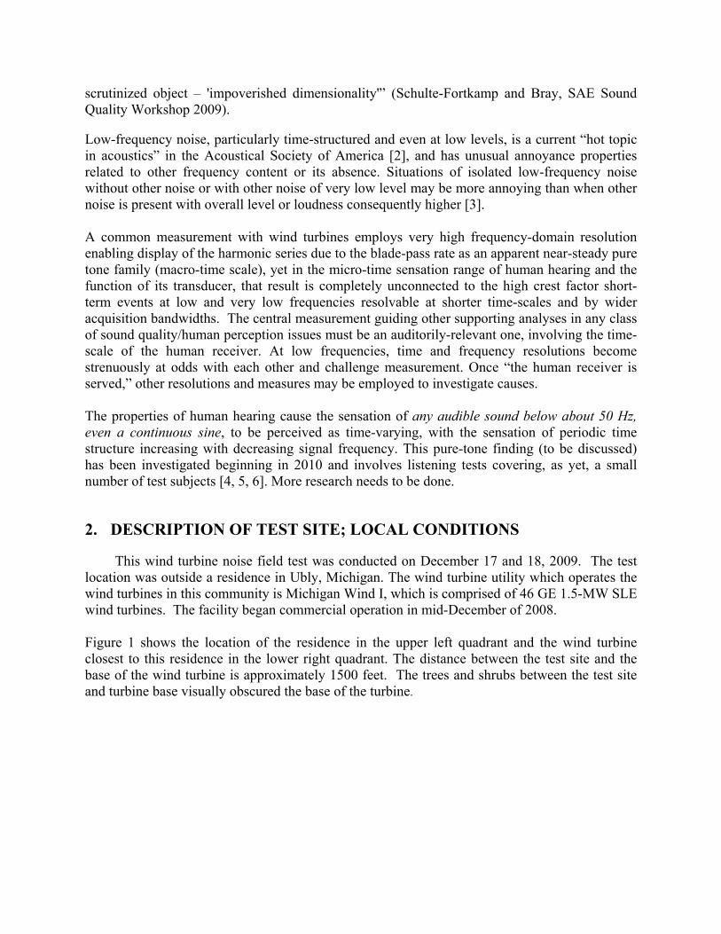
3.1 Measurement bandwidth For time-domain signals passed through band-pass filters, the measurement bandwidth affects both time and frequency resolutions: the wider a bandwidth, the better the time resolution but the poorer the frequency resolution. When frequency resolution is increased by assessing narrower bandwidths, time resolution decreases (impulse responses of narrower filters are longer than those of wider ones), potentially reducing auditorily-significant crest factors. For broadband signals, wider bandwidths contain more power and hence yield higher band-levels than the band-levels of subdivisions of the same signal frequency span into narrower bandwidths (the phenomenon of density level). Yet selection of the wider low-frequency hearing-appropriate measurement bandwidths preserves hearing-appropriate time resolution and yields a more correct representation of perceptually-important crest factors. Figure 2 shows two different types of measurement bandwidths: ANSI S1.11 1/3-octaves (also used in DIN and ISO loudness methods [9], and critical bands [10, 11, 12].

Figure 2 - Compared bandwidths (on log Hz scale): 1/3-octaves (upper), critical bands (lower). The 1/3-octaves chart also shows the synthesis of the lowest three critical bands in the psychoacoustic loudness measures ISO 532B, DIN 45631-1991 and DIN 45631/A1 from multiple 1/3-octave bands.

Critical bandwidths widen toward low frequency (on a log frequency scale), whereas constant-percentage bandwidths, such as the ANSI S1.11 1/3-octave filter bank, which retain a constant intervallic relationship, become narrower and narrower on a linear Hertz scale with decreasing frequency. Critical bandwidth filters used for measurement thereby exhibit more uniform and shorter impulse responses across frequency than do 1/n-octave filters, whose impulse responses grow longer and longer with decreasing frequency as shown in Figure 3. Among psychoacoustic models for time-varying loudness, the only currently standardized one, DIN 45631/A1 [12 op. cit.], is based upon critical bandwidths which have been shown to represent the time-response of human hearing [9 op. cit.]. Unfortunately, for historic reasons in standardization the lower-frequency critical bandwidths in DIN 45631/A1 as well as ISO 532B and DIN 45631-1991 are

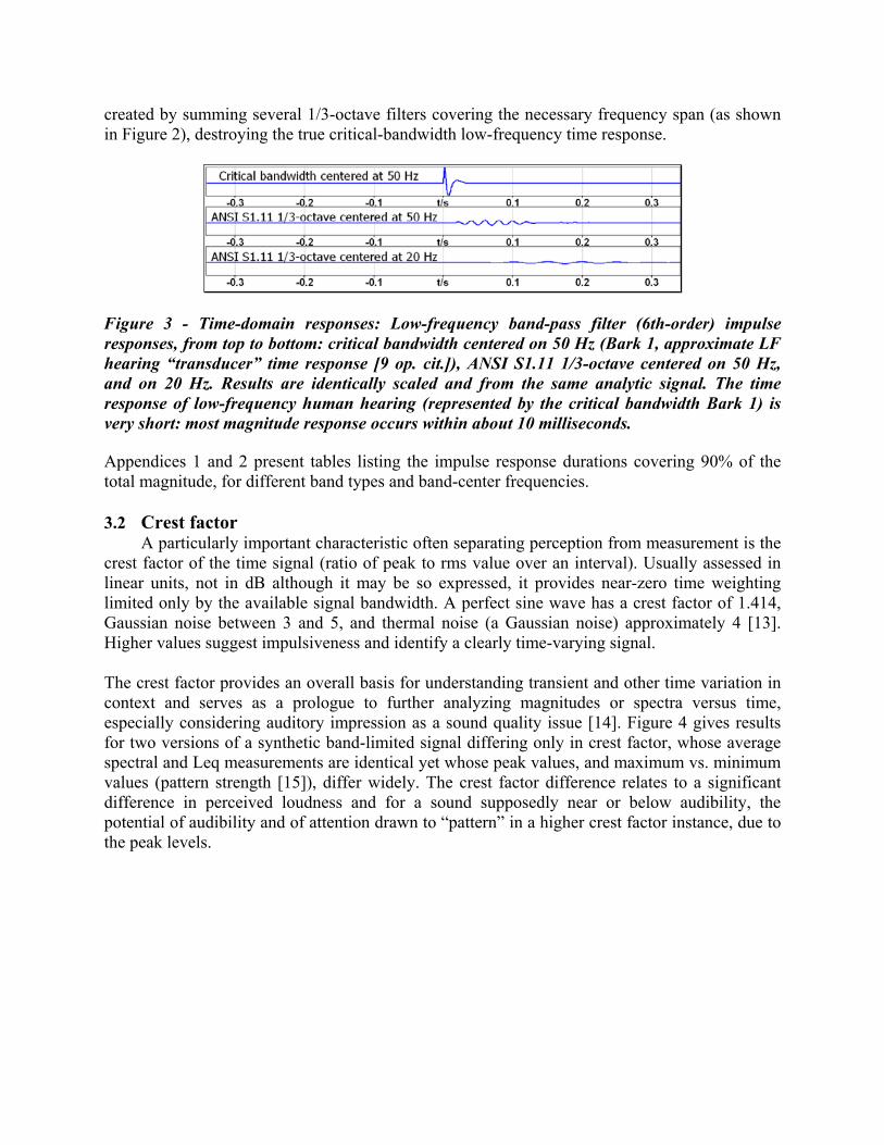
created by summing several 1/3-octave filters covering the necessary frequency span (as shown in Figure 2), destroying the true critical-bandwidth low-frequency time response.

Figure 3 - Time-domain responses: Low-frequency band-pass filter (6th-order) impulse responses, from top to bottom: critical bandwidth centered on 50 Hz (Bark 1, approximate LF hearing “transducer” time response [9 op. cit.]), ANSI S1.11 1/3-octave centered on 50 Hz, and on 20 Hz. Results are identically scaled and from the same analytic signal. The time response of low-frequency human hearing (represented by the critical bandwidth Bark 1) is very short: most magnitude response occurs within about 10 milliseconds.

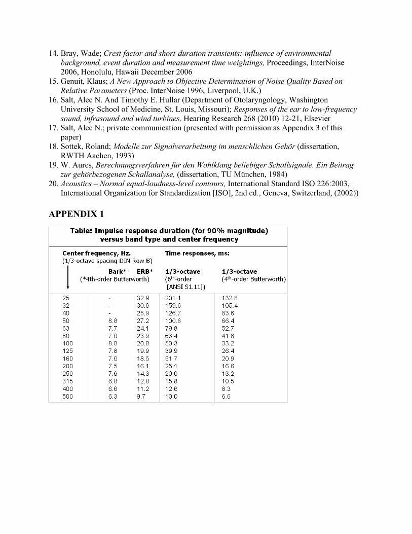
Appendices 1 and 2 present tables listing the impulse response durations covering 90% of the total magnitude, for different band types and band-center frequencies. 3.2 Crest factor A particularly important characteristic often separating perception from measurement is the crest factor of the time signal (ratio of peak to rms value over an interval). Usually assessed in linear units, not in dB although it may be so expressed, it provides near-zero time weighting limited only by the available signal bandwidth. A perfect sine wave has a crest factor of 1.414, Gaussian noise between 3 and 5, and thermal noise (a Gaussian noise) approximately 4 [13]. Higher values suggest impulsiveness and identify a clearly time-varying signal. The crest factor provides an overall basis for understanding transient and other time variation in context and serves as a prologue to further analyzing magnitudes or spectra versus time, especially considering auditory impression as a sound quality issue [14]. Figure 4 gives results for two versions of a synthetic band-limited signal differing only in crest factor, whose average spectral and Leq measurements are identical yet whose peak values, and maximum vs. minimum values (pattern strength [15]), differ widely. The crest factor difference relates to a significant difference in perceived loudness and for a sound supposedly near or below audibility, the potential of audibility and of attention drawn to “pattern” in a higher crest factor instance, due to the peak levels.

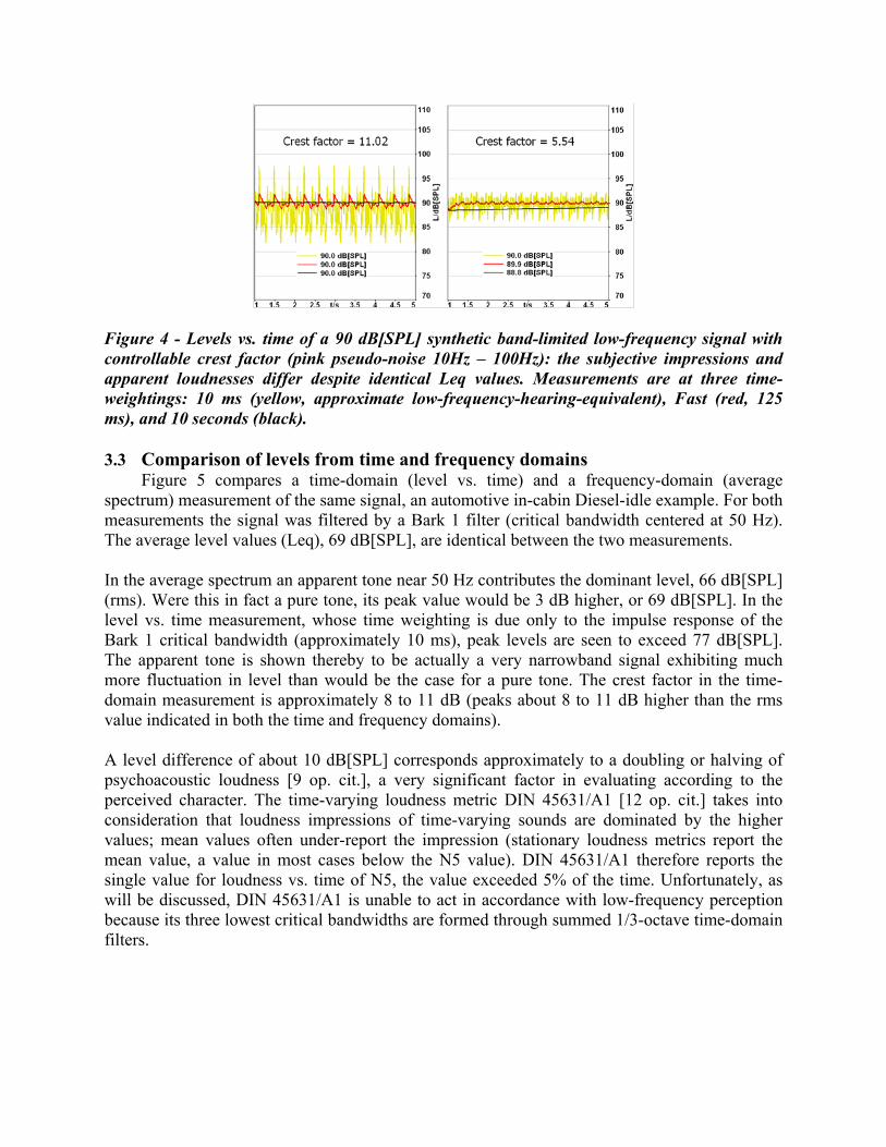
Figure 4 - Levels vs. time of a 90 dB[SPL] synthetic band-limited low-frequency signal with controllable crest factor (pink pseudo-noise 10Hz – 100Hz): the subjective impressions and apparent loudnesses differ despite identical Leq values. Measurements are at three time-weightings: 10 ms (yellow, approximate low-frequency-hearing-equivalent), Fast (red, 125 ms), and 10 seconds (black). 3.3 Comparison of levels from time and frequency domains Figure 5 compares a time-domain (level vs. time) and a frequency-domain (average spectrum) measurement of the same signal, an automotive in-cabin Diesel-idle example. For both measurements the signal was filtered by a Bark 1 filter (critical bandwidth centered at 50 Hz). The average level values (Leq), 69 dB[SPL], are identical between the two measurements. In the average spectrum an apparent tone near 50 Hz contributes the dominant level, 66 dB[SPL] (rms). Were this in fact a pure tone, its peak value would be 3 dB higher, or 69 dB[SPL]. In the level vs. time measurement, whose time weighting is due only to the impulse response of the Bark 1 critical bandwidth (approximately 10 ms), peak levels are seen to exceed 77 dB[SPL]. The apparent tone is shown thereby to be actually a very narrowband signal exhibiting much more fluctuation in level than would be the case for a pure tone. The crest factor in the time-domain measurement is approximately 8 to 11 dB (peaks about 8 to 11 dB higher than the rms value indicated in both the time and frequency domains). A level difference of about 10 dB[SPL] corresponds approximately to a doubling or halving of psychoacoustic loudness [9 op. cit.], a very significant factor in evaluating according to the perceived character. The time-varying loudness metric DIN 45631/A1 [12 op. cit.] takes into consideration that loudness impressions of time-varying sounds are dominated by the higher values; mean values often under-report the impression (stationary loudness metrics report the mean value, a value in most cases below the N5 value). DIN 45631/A1 therefore reports the single value for loudness vs. time of N5, the value exceeded 5% of the time. Unfortunately, as will be discussed, DIN 45631/A1 is unable to act in accordance with low-frequency perception because its three lowest critical bandwidths are formed through summed 1/3-octave time-domain filters.

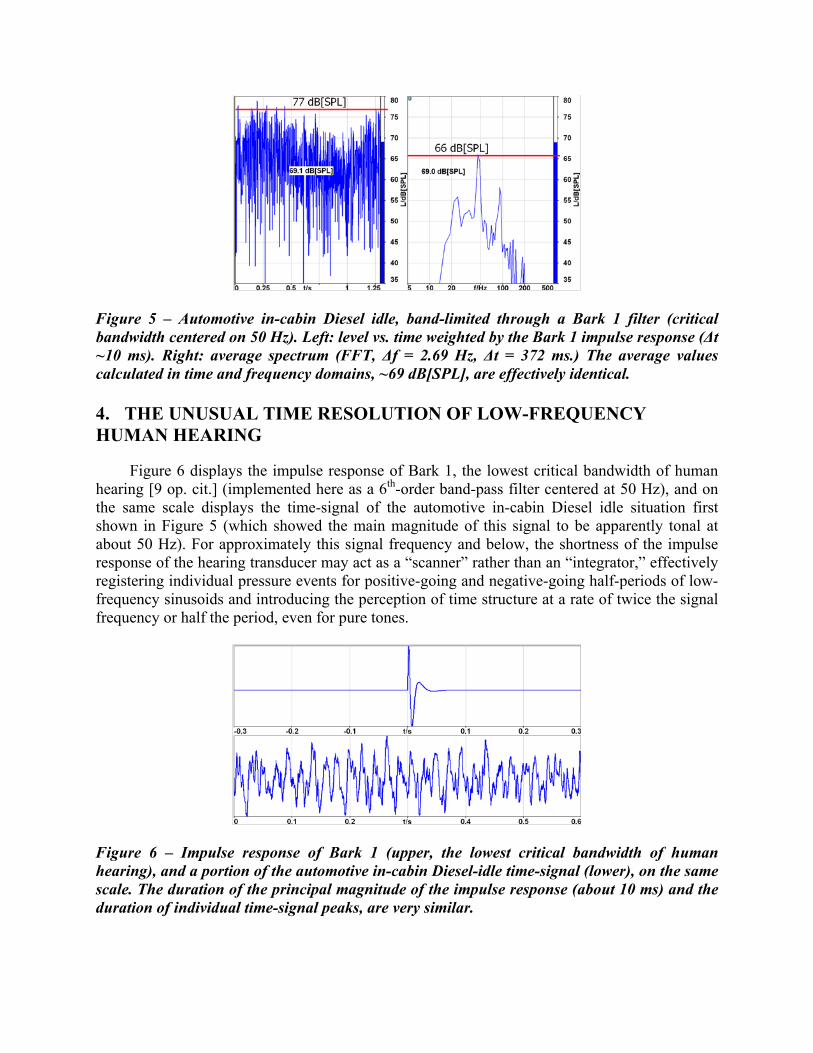
Figure 5 – Automotive in-cabin Diesel idle, band-limited through a Bark 1 filter (critical bandwidth centered on 50 Hz). Left: level vs. time weighted by the Bark 1 impulse response (∆t ~10 ms). Right: average spectrum (FFT, ∆f = 2.69 Hz, ∆t = 372 ms.) The average values calculated in time and frequency domains, ~69 dB[SPL], are effectively identical. 4. THE UNUSUAL TIME RESOLUTION OF LOW-FREQUENCY HUMAN HEARING

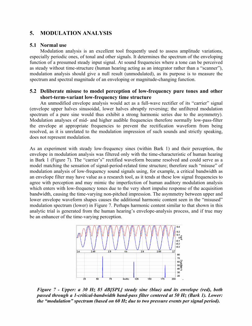
Figure 6 displays the impulse response of Bark 1, the lowest critical bandwidth of human hearing [9 op. cit.] (implemented here as a 6th-order band-pass filter centered at 50 Hz), and on the same scale displays the time-signal of the automotive in-cabin Diesel idle situation first shown in Figure 5 (which showed the main magnitude of this signal to be apparently tonal at about 50 Hz). For approximately this signal frequency and below, the shortness of the impulse response of the hearing transducer may act as a “scanner” rather than an “integrator,” effectively registering individual pressure events for positive-going and negative-going half-periods of low-frequency sinusoids and introducing the perception of time structure at a rate of twice the signal frequency or half the period, even for pure tones.

Figure 6 – Impulse response of Bark 1 (upper, the lowest critical bandwidth of human hearing), and a portion of the automotive in-cabin Diesel-idle time-signal (lower), on the same scale. The duration of the principal magnitude of the impulse response (about 10 ms) and the duration of individual time-signal peaks, are very similar.

5. MODULATION ANALYSIS 5.1 Normal use Modulation analysis is an excellent tool frequently used to assess amplitude variations, especially periodic ones, of tonal and other signals. It determines the spectrum of the enveloping function of a presumed steady input signal. At sound frequencies where a tone can be perceived as steady without time-structure (human hearing acting as an integrator rather than a “scanner”), modulation analysis should give a null result (unmodulated), as its purpose is to measure the spectrum and spectral magnitude of an enveloping or magnitude-changing function. 5.2 Deliberate misuse to model perception of low-frequency pure tones and other

short-term-variant low-frequency time structure An unmodified envelope analysis would act as a full-wave rectifier of its “carrier” signal (envelope upper halves sinusoidal, lower halves abruptly reversing; the unfiltered modulation spectrum of a pure sine would thus exhibit a strong harmonic series due to the asymmetry). Modulation analyses of mid- and higher audible frequencies therefore normally low-pass-filter the envelope at appropriate frequencies to prevent the rectification waveform from being resolved, as it is unrelated to the modulation impression of such sounds and strictly speaking, does not represent modulation. As an experiment with steady low-frequency sines (within Bark 1) and their perception, the envelope in modulation analysis was filtered only with the time-characteristic of human hearing in Bark 1 (Figure 7). The “carrier’s” rectified waveform became resolved and could serve as a model matching the sensation of signal-period-related time structure; therefore such “misuse” of modulation analysis of low-frequency sound signals using, for example, a critical bandwidth as an envelope filter may have value as a research tool, as it tends at these low signal frequencies to agree with perception and may mimic the imperfection of human auditory modulation analysis which enters with low-frequency tones due to the very short impulse response of the acquisition bandwidth, causing the time-varying non-pitched impression. The asymmetry between upper and lower envelope waveform shapes causes the additional harmonic content seen in the “misused” modulation spectrum (lower) in Figure 7. Perhaps harmonic content similar to that shown in this analytic trial is generated from the human hearing’s envelope-analysis process, and if true may be an enhancer of the time-varying perception.

.

Figure 7 - Upper: a 30 Hz 85 dB[SPL] steady sine (blue) and its envelope (red), both passed through a 1-critical-bandwidth band-pass filter centered at 50 Hz (Bark 1). Lower: the “modulation” spectrum (based on 60 Hz due to two pressure events per signal period).

5.3 Application The authors suggest that more research be undertaken regarding this hypothesis. For any demonstrable ear-transducer activity (whether resulting in audition or not) [16, 17] responding to low and very low frequency signals, the authors suggest using modulation analysis in this "unorthodox" manner tied to the impulse response duration of the acquisition critical bandwidth, to model the human-receiver behavior. 6. WIND TURBINE RESULTS

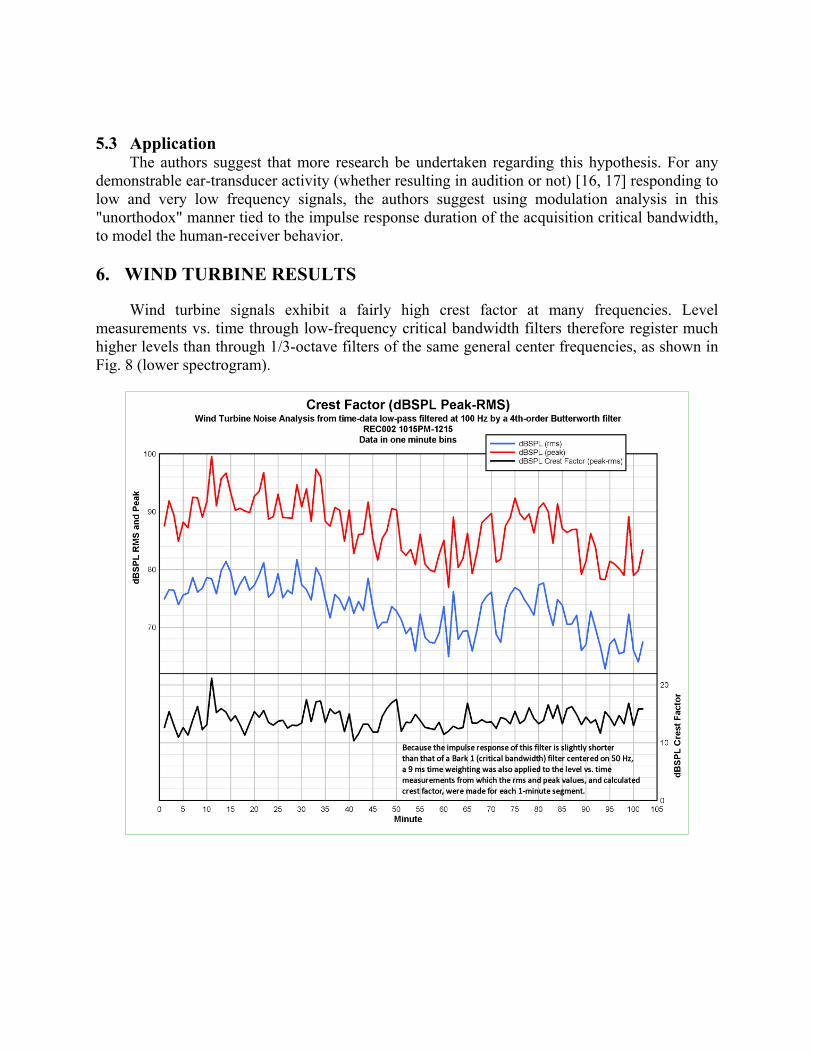
Wind turbine signals exhibit a fairly high crest factor at many frequencies. Level measurements vs. time through low-frequency critical bandwidth filters therefore register much higher levels than through 1/3-octave filters of the same general center frequencies, as shown in Fig. 8 (lower spectrogram).

f/Hz

20

100

500

2k

10k

t/s1000 2000 4000 5000 6000L/dB[SPL]30 40 50 70 80 90

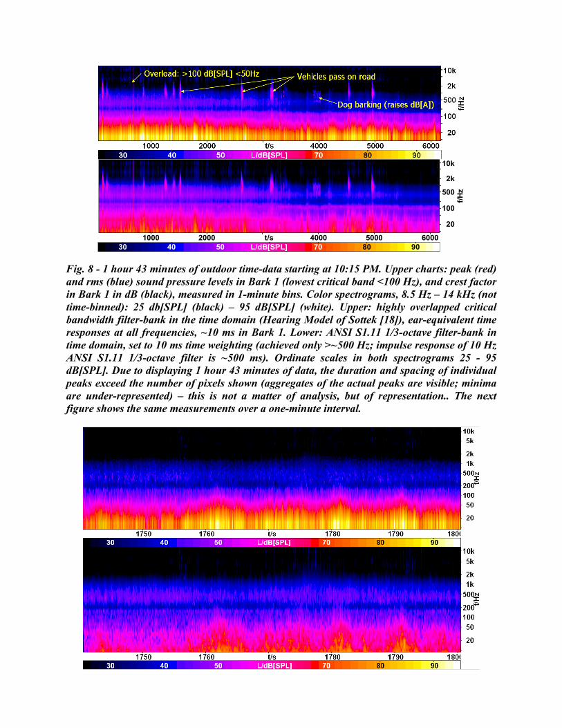
Fig. 8 - 1 hour 43 minutes of outdoor time-data starting at 10:15 PM. Upper charts: peak (red) and rms (blue) sound pressure levels in Bark 1 (lowest critical band <100 Hz), and crest factor in Bark 1 in dB (black), measured in 1-minute bins. Color spectrograms, 8.5 Hz – 14 kHz (not time-binned): 25 db[SPL] (black) – 95 dB[SPL] (white). Upper: highly overlapped critical bandwidth filter-bank in the time domain (Hearing Model of Sottek [18]), ear-equivalent time responses at all frequencies, ~10 ms in Bark 1. Lower: ANSI S1.11 1/3-octave filter-bank in time domain, set to 10 ms time weighting (achieved only >~500 Hz; impulse response of 10 Hz ANSI S1.11 1/3-octave filter is ~500 ms). Ordinate scales in both spectrograms 25 - 95 dB[SPL]. Due to displaying 1 hour 43 minutes of data, the duration and spacing of individual peaks exceed the number of pixels shown (aggregates of the actual peaks are visible; minima are under-represented) – this is not a matter of analysis, but of representation.. The next figure shows the same measurements over a one-minute interval.

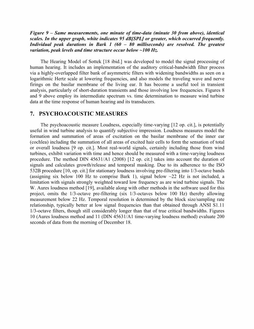
Figure 9 – Same measurements, one minute of time-data (minute 30 from above), identical scales. In the upper graph, white indicates 95 dB[SPL] or greater, which occurred frequently. Individual peak durations in Bark 1 (60 – 80 milliseconds) are resolved. The greatest variation, peak levels and time structure occur below ~100 Hz. The Hearing Model of Sottek [18 ibid.] was developed to model the signal processing of human hearing. It includes an implementation of the auditory critical-bandwidth filter process via a highly-overlapped filter bank of asymmetric filters with widening bandwidths as seen on a logarithmic Hertz scale at lowering frequencies, and also models the traveling wave and nerve firings on the basilar membrane of the living ear. It has become a useful tool in transient analysis, particularly of short-duration transients and those involving low frequencies. Figures 8 and 9 above employ its intermediate spectrum vs. time determination to measure wind turbine data at the time response of human hearing and its transducers. 7. PSYCHOACOUSTIC MEASURES

The psychoacoustic measure Loudness, especially time-varying [12 op. cit.], is potentially useful in wind turbine analysis to quantify subjective impression. Loudness measures model the formation and summation of areas of excitation on the basilar membrane of the inner ear (cochlea) including the summation of all areas of excited hair cells to form the sensation of total or overall loudness [9 op. cit.]. Most real-world signals, certainly including those from wind turbines, exhibit variation with time and hence should be measured with a time-varying loudness procedure. The method DIN 45631/A1 (2008) [12 op. cit.] takes into account the duration of signals and calculates growth/release and temporal masking. Due to its adherence to the ISO 532B procedure [10, op. cit.] for stationary loudness involving pre-filtering into 1/3-octave bands (assigning six below 100 Hz to comprise Bark 1), signal below ~22 Hz is not included, a limitation with signals strongly weighted toward low frequency as are wind turbine signals. The W. Aures loudness method [19], available along with other methods in the software used for this project, omits the 1/3-octave pre-filtering (six 1/3-octaves below 100 Hz) thereby allowing measurement below 22 Hz. Temporal resolution is determined by the block size/sampling rate relationship, typically better at low signal frequencies than that obtained through ANSI S1.11 1/3-octave filters, though still considerably longer than that of true critical bandwidths. Figures 10 (Aures loudness method and 11 (DIN 45631/A1 time-varying loudness method) evaluate 200 seconds of data from the morning of December 18.

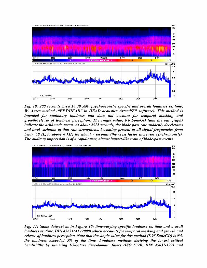
Fig. 10: 200 seconds circa 10:30 AM: psychoacoustic specific and overall loudness vs. time, W. Aures method (“FFT/HEAD” in HEAD acoustics ArtemiS™ software). This method is intended for stationary loudness and does not account for temporal masking and growth/release of loudness perception. The single value, 6.6 SoneGD (and the bar graph) indicate the arithmetic mean. At about 2312 seconds, the blade pass rate suddenly decelerates and level variation at that rate strengthens, becoming present at all signal frequencies from below 50 Hz to above 6 kHz for about 7 seconds (the crest factor increases synchronously). The auditory impression is of a rapid-onset, almost impact-like train of blade-pass events.

Fig. 11: Same data-set as in Figure 10: time-varying specific loudness vs. time and overall loudness vs. time, DIN 45631/A1 (2008) which accounts for temporal masking and growth and release of loudness perception. Note that the single value for this method (5.95 SoneGD) is N5, the loudness exceeded 5% of the time. Loudness methods deriving the lowest critical bandwidths by summing 1/3-octave time-domain filters (ISO 532B, DIN 45631-1991 and

45631/A1) degrade the true impulse responses of these critical bandwidths and therefore under-represent the true crest factors and momentary loudness contributions of signals in these bands.

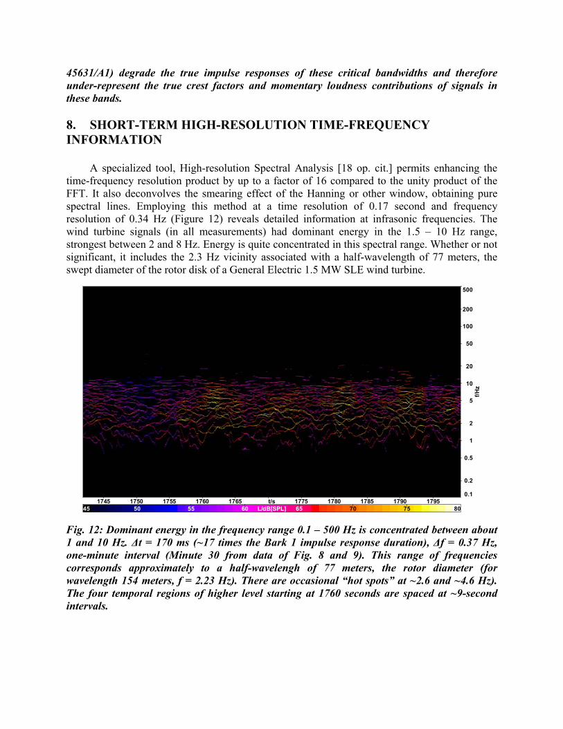
8. SHORT-TERM HIGH-RESOLUTION TIME-FREQUENCY INFORMATION A specialized tool, High-resolution Spectral Analysis [18 op. cit.] permits enhancing the time-frequency resolution product by up to a factor of 16 compared to the unity product of the FFT. It also deconvolves the smearing effect of the Hanning or other window, obtaining pure spectral lines. Employing this method at a time resolution of 0.17 second and frequency resolution of 0.34 Hz (Figure 12) reveals detailed information at infrasonic frequencies. The wind turbine signals (in all measurements) had dominant energy in the 1.5 – 10 Hz range, strongest between 2 and 8 Hz. Energy is quite concentrated in this spectral range. Whether or not significant, it includes the 2.3 Hz vicinity associated with a half-wavelength of 77 meters, the swept diameter of the rotor disk of a General Electric 1.5 MW SLE wind turbine.

f/Hz

0.1

0.2

0.5

1

2

5

10

20

50

100

200

500

t/s1745 1750 1755 1760 1765 1775 1780 1785 1790 1795L/dB[SPL]45 50 55 60 65 70 75 80

Fig. 12: Dominant energy in the frequency range 0.1 – 500 Hz is concentrated between about 1 and 10 Hz. ∆t = 170 ms (~17 times the Bark 1 impulse response duration), ∆f = 0.37 Hz, one-minute interval (Minute 30 from data of Fig. 8 and 9). This range of frequencies corresponds approximately to a half-wavelengh of 77 meters, the rotor diameter (for wavelength 154 meters, f = 2.23 Hz). There are occasional “hot spots” at ~2.6 and ~4.6 Hz). The four temporal regions of higher level starting at 1760 seconds are spaced at ~9-second intervals.

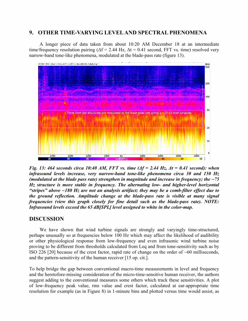
9. OTHER TIME-VARYING LEVEL AND SPECTRAL PHENOMENA A longer piece of data taken from about 10:20 AM December 18 at an intermediate time/frequency resolution pairing (∆f = 2.44 Hz, ∆t = 0.41 second, FFT vs. time) resolved very narrow-band tone-like phenomena, modulated at the blade-pass rate (figure 13).

Fig. 13: 464 seconds circa 10:40 AM, FFT vs. time (∆f = 2.44 Hz, ∆t = 0.41 second): when infrasound levels increase, very narrow-band tone-like phenomena circa 30 and 150 Hz (modulated at the blade pass rate) strengthen in magnitude and increase in frequency; the ~75 Hz structure is more stable in frequency. The alternating low- and higher-level horizontal “stripes” above ~180 Hz are not an analysis artifact; they may be a comb-filter effect due to the ground reflection. Amplitude change at the blade-pass rate is visible at many signal frequencies (view this graph closely for fine detail such as the blade-pass rate). NOTE: Infrasound levels exceed the 65 dB[SPL] level assigned to white in the color-map. DISCUSSION

We have shown that wind turbine signals are strongly and varyingly time-structured, perhaps unusually so at frequencies below 100 Hz which may affect the likelihood of audibility or other physiological response from low-frequency and even infrasonic wind turbine noise proving to be different from thresholds calculated from Leq and from tone-sensitivity such as by ISO 226 [20] because of the crest factor, rapid rate of change on the order of ~60 milliseconds, and the pattern-sensitivity of the human receiver [15 op. cit.]. To help bridge the gap between conventional macro-time measurements in level and frequency and the heretofore-missing consideration of the micro-time-sensitive human receiver, the authors suggest adding to the conventional measures some others which track these sensitivities. A plot of low-frequency peak value, rms value and crest factor, calculated at ear-appropriate time resolution for example (as in Figure 8) in 1-minute bins and plotted versus time would assist, as

would statistic tabulations from them such as the peak, rms and crest factor values exceeded 50%, 5%, and 1% of the time. We hope that we have provided useful information on the nature of wind turbine noise, and encourage others to engage in further research aided by these results. ACKNOWLEDGMENTS

The authors would like to thank colleagues (of author Bray) Dr.-Ing. Roland Sottek, André Fiebig, Georg Caspary and Prof. Dr.-Ing. Klaus Genuit for support of this avenue of investigation, productive discussions, initial small-scale listening tests regarding the perception of time structure from low-frequency pure tones. The authors also thank Prof. Dr. Brigitte Schulte-Fortkamp for her encouragement of this effort, and Charles Ebbing and Dr. Malcolm Swinbanks for productive discussions. REFERENCES 1. Schafer, Raymond Murray; The Tuning of the World, University of Pennsylvania Press,

1977; ISBN 081221109X 2. Acoustical Society of America, Interdisciplinary Hot Topics in Acoustics, 2010 3. Krahe, D.; Why is sharp-limited low-frequency noise extremely annoying? JASA

123(5):3569, May 2008 4. HEAD acoustics 2010 December: W. Bray (US), R. Sottek, A. Fiebig (Germany), private

communications 5. Bray, Wade; Sensation and measurement of low and very low frequency time-varying sounds

in accordance with the very short impulse response of low-frequency human hearing, Proceedings, Society of Automotive Engineers Noise and Vibration Conference 2011, May 2011, Grand Rapids, Michigan

6. Bray, Wade; Perceptions, and measurement implications, of time structure in low-frequency sounds, Proceedings, Noise-Con 2011, July 2011, Portland, Oregon

7. http://www.head-acoustics.de/downloads/eng/application_notes/Equalization_brochure.pdf 8. Bray, Wade R.; Binaural measurements in an Information Technology acoustic program,

Proceedings, Internoise 2009, August, 2009, Ottawa, Ontario, Canada 9. Zwicker, Eberhard and Hugo Fastl; Psychoacoustics: Facts and Models, Springer-Verlag,

Germany, (1999) 10. Acoustics – Method for calculating loudness level, International Standard ISO 532B:1975,

International Organization for Standardization [ISO], Geneva, Switzerland (1975) 11. DIN 45631 (1991), “Berechnung des Lautstärkepegels und der Lautheit aus dem

Geräuschspektrum – Verfahren nach E. Zwicker,” Deutsche Institut für Normung e. V., (1991)

12. DIN 45631/A1: (German): Berechnung des Lautstärkepegels und der Lautheit aus dem Geräuschspektrum - Verfahren nach E. Zwicker - Änderung 1: Berechnung der Lautheit zeitvarianter Geräusche (English): Calculation of loudness level and loudness from the sound spectrum - Zwicker method - Amendment 1: Calculation of the loudness of time-variant sound, Beuth Verlag GmbH, (2010-03)

13. Ott, Henry; Noise Reduction Techniques in Electronic Systems, New York, John Wiley and Sons, 1976, 1998

14. Bray, Wade; Crest factor and short-duration transients: influence of environmental background, event duration and measurement time weightings, Proceedings, InterNoise 2006, Honolulu, Hawaii December 2006

15. Genuit, Klaus; A New Approach to Objective Determination of Noise Quality Based on Relative Parameters (Proc. InterNoise 1996, Liverpool, U.K.)

16. Salt, Alec N. And Timothy E. Hullar (Department of Otolaryngology, Washington University School of Medicine, St. Louis, Missouri); Responses of the ear to low-frequency sound, infrasound and wind turbines, Hearing Research 268 (2010) 12-21, Elsevier

17. Salt, Alec N.; private communication (presented with permission as Appendix 3 of this paper)

18. Sottek, Roland; Modelle zur Signalverarbeitung im menschlichen Gehör (dissertation, RWTH Aachen, 1993)

19. W. Aures, Berechnungsverfahren für den Wohlklang beliebiger Schallsignale. Ein Beitrag zur gehörbezogenen Schallanalyse, (dissertation, TU München, 1984)

20. Acoustics – Normal equal-loudness-level contours, International Standard ISO 226:2003, International Organization for Standardization [ISO], 2nd ed., Geneva, Switzerland, (2002))

APPENDIX 1

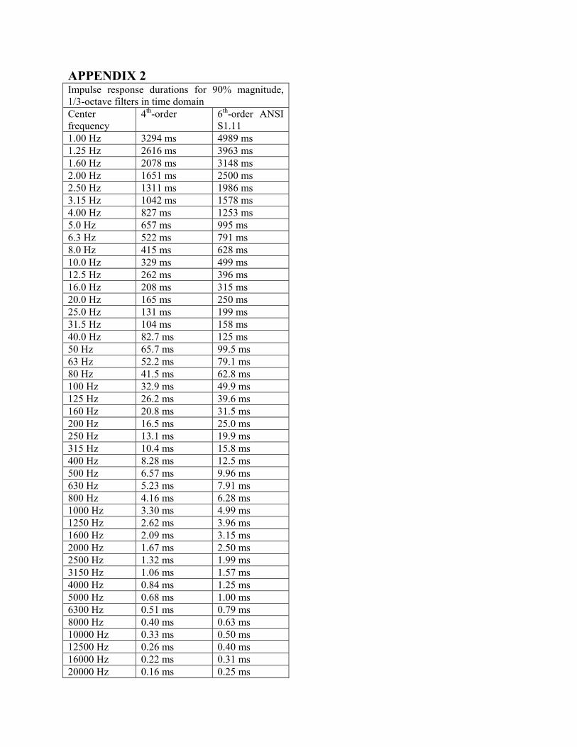
APPENDIX 2 Impulse response durations for 90% magnitude, 1/3-octave filters in time domain Center frequency

4th-order 6th-order ANSI S1.11

1.00 Hz 3294 ms 4989 ms 1.25 Hz 2616 ms 3963 ms 1.60 Hz 2078 ms 3148 ms 2.00 Hz 1651 ms 2500 ms 2.50 Hz 1311 ms 1986 ms 3.15 Hz 1042 ms 1578 ms 4.00 Hz 827 ms 1253 ms 5.0 Hz 657 ms 995 ms 6.3 Hz 522 ms 791 ms 8.0 Hz 415 ms 628 ms 10.0 Hz 329 ms 499 ms 12.5 Hz 262 ms 396 ms 16.0 Hz 208 ms 315 ms 20.0 Hz 165 ms 250 ms 25.0 Hz 131 ms 199 ms 31.5 Hz 104 ms 158 ms 40.0 Hz 82.7 ms 125 ms 50 Hz 65.7 ms 99.5 ms 63 Hz 52.2 ms 79.1 ms 80 Hz 41.5 ms 62.8 ms 100 Hz 32.9 ms 49.9 ms 125 Hz 26.2 ms 39.6 ms 160 Hz 20.8 ms 31.5 ms 200 Hz 16.5 ms 25.0 ms 250 Hz 13.1 ms 19.9 ms 315 Hz 10.4 ms 15.8 ms 400 Hz 8.28 ms 12.5 ms 500 Hz 6.57 ms 9.96 ms 630 Hz 5.23 ms 7.91 ms 800 Hz 4.16 ms 6.28 ms 1000 Hz 3.30 ms 4.99 ms 1250 Hz 2.62 ms 3.96 ms 1600 Hz 2.09 ms 3.15 ms 2000 Hz 1.67 ms 2.50 ms 2500 Hz 1.32 ms 1.99 ms 3150 Hz 1.06 ms 1.57 ms 4000 Hz 0.84 ms 1.25 ms 5000 Hz 0.68 ms 1.00 ms 6300 Hz 0.51 ms 0.79 ms 8000 Hz 0.40 ms 0.63 ms 10000 Hz 0.33 ms 0.50 ms 12500 Hz 0.26 ms 0.40 ms 16000 Hz 0.22 ms 0.31 ms 20000 Hz 0.16 ms 0.25 ms

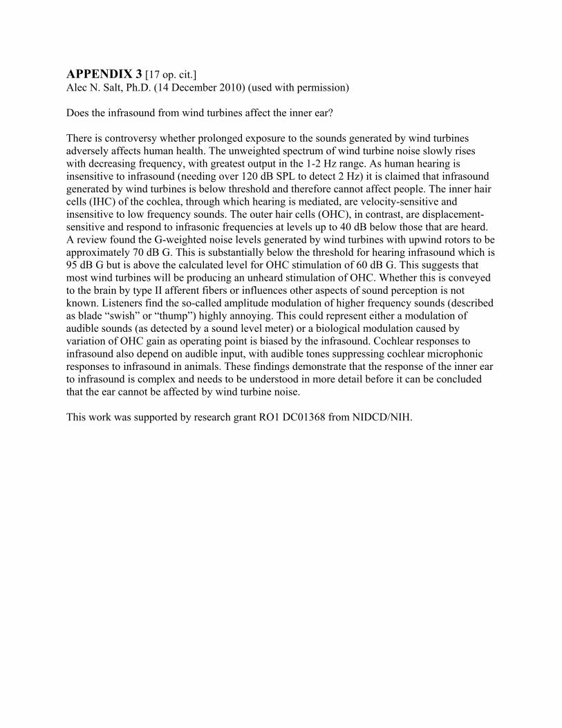
APPENDIX 3 [17 op. cit.] Alec N. Salt, Ph.D. (14 December 2010) (used with permission) Does the infrasound from wind turbines affect the inner ear? There is controversy whether prolonged exposure to the sounds generated by wind turbines adversely affects human health. The unweighted spectrum of wind turbine noise slowly rises with decreasing frequency, with greatest output in the 1-2 Hz range. As human hearing is insensitive to infrasound (needing over 120 dB SPL to detect 2 Hz) it is claimed that infrasound generated by wind turbines is below threshold and therefore cannot affect people. The inner hair cells (IHC) of the cochlea, through which hearing is mediated, are velocity-sensitive and insensitive to low frequency sounds. The outer hair cells (OHC), in contrast, are displacement-sensitive and respond to infrasonic frequencies at levels up to 40 dB below those that are heard. A review found the G-weighted noise levels generated by wind turbines with upwind rotors to be approximately 70 dB G. This is substantially below the threshold for hearing infrasound which is 95 dB G but is above the calculated level for OHC stimulation of 60 dB G. This suggests that most wind turbines will be producing an unheard stimulation of OHC. Whether this is conveyed to the brain by type II afferent fibers or influences other aspects of sound perception is not known. Listeners find the so-called amplitude modulation of higher frequency sounds (described as blade “swish” or “thump”) highly annoying. This could represent either a modulation of audible sounds (as detected by a sound level meter) or a biological modulation caused by variation of OHC gain as operating point is biased by the infrasound. Cochlear responses to infrasound also depend on audible input, with audible tones suppressing cochlear microphonic responses to infrasound in animals. These findings demonstrate that the response of the inner ear to infrasound is complex and needs to be understood in more detail before it can be concluded that the ear cannot be affected by wind turbine noise. This work was supported by research grant RO1 DC01368 from NIDCD/NIH.