dynamic modeling of household electricity consumption
TRANSCRIPT

Aalto University
School of Electrical Engineering
Department of Automation and Systems Technology
Tomi Sorasalmi
Dynamic Modeling of Household ElectricityConsumption
Master’s ThesisEspoo, August 13, 2012
Supervisor: Kai Zenger, Prof.Instructors: Robert Weiss, Lic.Sc. (Tech.)
Jean-Peter Ylen, D.Sc. (Tech.)

Aalto UniversitySchool of Electrical EngineeringDepartment of Automation and Systems Technology
ABSTRACT OFMASTER’S THESIS
Author: Tomi Sorasalmi
Title:Dynamic Modeling of Household Electricity Consumption
Date: August 13, 2012 Pages: xii + 120
Professorship: Control Engineering Code: AS-74
Supervisor: Kai Zenger, Prof.
Instructors: Robert Weiss, Lic.Sc. (Tech.)Jean-Peter Ylen, D.Sc. (Tech.)
The change in household electricity consumption affects many parties in the elec-tricity business, and therefore more accurate tools for analysing the possible out-comes are needed. In this thesis, the objective is to implement a tool capable ofproducing future scenarios of the electricity consumption and load profile changesusing structural modeling techniques. The tool consists of two simulation models,which are integrated and can be used separately or as one.
The long-term model, describing household electricity consumption change dur-ing the next 40 years, is made using system dynamics approach. The short-termmodel, describing daily and weekly load profiles, is made using bottom-up ap-proach. By dividing the problem into two models the benefits from both top-downand bottom-up approaches can be used and the problems related to stiff systemscan be avoided.
The long-term model is validated against historical data and with expert evalu-ations. The model can be used for generating scenarios of the future householdelectricity consumption and the user can change parameters by using the imple-mented user interface.
Integration of the two different approaches was successful and the model is ableto address how different changes in the long-term model, such as the number andenergy efficiency of appliances, are affecting the load profiles. However, the short-term model is incomplete and therefore the simulation results are only indicative.
Keywords: Electricity consumption, dynamic systems, system dynamics,load profile, smart grid, demand-side management, demandresponse, consumer behavior, households, tariff structures
Language: English
ii

Aalto-yliopistoSahkotekniikan korkeakouluAutomaatio- ja systeemitekniikan laitos
DIPLOMITYONTIIVISTELMA
Tekija: Tomi Sorasalmi
Tyon nimi:Kotitalouksien sahkonkulutuksen dynaaminen mallinnus
Paivays: 13. elokuuta 2012 Sivumaara: xii + 120
Professuuri: Systeemitekniikka Koodi: AS-74
Valvoja: Kai Zenger, Prof.
Ohjaajat: Robert Weiss, TkLJean-Peter Ylen, TkT
Kotitalouksien sahkonkulutuksen kehitys vaikuttaa eri osapuoliinsahkomarkkinoilla, jonka takia sahkonkulutuksen tarkempi analysointi ontarpeellista. Tarkoitus on tehda simulointityokalu, jolla on mahdollista testataerilaisia skenaarioita kotitalouksien kokonaissahkonkulutuksen ja kuormi-tuskayrien kehityksesta. Tyossa on kaytetty rakenteellisia mallinnusmenetelmia.Tyokalussa kaksi eri simulointimallia on integroitu yhdeksi kokonaisuudeksi.Malleja voidaan kayttaa yhdessa tai erikseen.
Pitkan aikavalin malli, joka tarkastelee kotitalouksien sahkonkulutuksen muutos-ta seuraavan 40 vuoden aikana, on tehty kayttaen systeemidynaamista mallin-nusmenetelmaa. Lyhyen aikavalin malli, joka kuvaa paiva- ja viikkokuormitus-profiileja, on tehty bottom-up -ajattelun pohjalta.
Pitkan aikavalin malli on validoitu historiadataa vasten seka asiantuntija-arvioilla. Malli pystyy tuottamaan skenaarioita kotitalouksien sahkonkulutuksenkehityksesta; kayttaja voi halutessaan muuttaa mallin parametrejakayttoliittyman avulla.
Kahden eri mallinnusmenetelman integrointi onnistui hyvin ja mallilla voi testa-ta kuinka muutokset pitkan aikavalin mallissa, kuten kotitalouslaitteiden maaraja energiatehokkuus, vaikuttavat kuormitusprofiileihin. Lyhyen aikavalin malli eikuitenkaan ole viela valmis, joten simulointituloksia voi pitaa pelkastaan suuntaaantavina.
Asiasanat: Sahkonkulutus, dynaamiset systeemit, systeemidyna-miikka, kuormituskayra, alykkaat sahkoverkot, kulutta-jakayttaytyminen, kysyntajousto, kysynnanohjaus, tariffira-kenteet
Kieli: Englanti
iii

Acknowledgements
This Master’s Thesis is done in the System Dynamics team at VTT TechnicalResearch Centre of Finland.
I wish to thank my instructors Lic.Sc. Robert Weiss and D.Sc. Jean-PeterYlen for their guidance and insight. I would also like to thank my supervisor,professor Kai Zenger, and my colleagues for their help and comments.
Espoo, August 13, 2012
Tomi Sorasalmi
iv

Abbreviations and Acronyms
Abbreviations
AMR Automatic Meter ReadingBAU Business-as-usual scenarioCET Central European TimeCPP Critical Peak PricingDR Demand ResponseDSM Demand-side ManagementEU European UnionGDP Gross Domestic ProductGSHP Ground Source Heat PumpHEV Hybrid and Electric VehicleHVAC Heat, Ventilation, and Air ConditioningLED Light-Emitting DiodeRTP Real-time PricingToU Time-of-UseTSO Transmission System OperatorVBA Visual Basic for ApplicationsVTT VTT Technical Research Centre of Finland
Terminology
Distributor Transfers the electricity from the main grid to the end-user. Owner of the transmission net.
Load Profile A graph describing the variations in the electrical loadversus time.
Producer Generates electricity in the power plants.Scenario A possible future path of development.Smart meter Measures electricity consumption in a given time inter-
val and delivers information for monitoring and billingpurposes.
Spot/System Price Electricity price for a given time interval, typically forone hour.
Supplier Buys electricity from Nord Pool and sells it to the end-users.
TSO Transmission System Operator. Is responsible of themain grid. In Finland the TSO is Fingrid.
v

Contents
Acknowledgements iv
Abbreviations and Terminology v
List of Figures ix
1 Introduction 11.1 Background . . . . . . . . . . . . . . . . . . . . . . . . . . . . . . 11.2 Research Objectives . . . . . . . . . . . . . . . . . . . . . . . . . . 21.3 Structure of the Thesis . . . . . . . . . . . . . . . . . . . . . . . . 2
2 Electricity Markets 42.1 Introduction . . . . . . . . . . . . . . . . . . . . . . . . . . . . . . 42.2 Nord Pool . . . . . . . . . . . . . . . . . . . . . . . . . . . . . . . 7
2.2.1 Market Participants in Nord Pool . . . . . . . . . . . . . . 82.2.2 Day-ahead Market - Elspot . . . . . . . . . . . . . . . . . 92.2.3 Intraday Market - Elbas . . . . . . . . . . . . . . . . . . . 102.2.4 Financial Market, Nasdaq OMX Commodities . . . . . . . 10
2.3 Nord Pool Evolution and Smart Grid . . . . . . . . . . . . . . . . 102.3.1 Smart Grid . . . . . . . . . . . . . . . . . . . . . . . . . . 112.3.2 Tariff Structures . . . . . . . . . . . . . . . . . . . . . . . 12
3 System Dynamics 133.1 Introduction . . . . . . . . . . . . . . . . . . . . . . . . . . . . . . 133.2 Causal Loop Diagrams . . . . . . . . . . . . . . . . . . . . . . . . 153.3 Stocks and Flows . . . . . . . . . . . . . . . . . . . . . . . . . . . 163.4 Properties of Dynamic Systems . . . . . . . . . . . . . . . . . . . 16
3.4.1 Feedback Loops . . . . . . . . . . . . . . . . . . . . . . . . 163.4.2 Delays . . . . . . . . . . . . . . . . . . . . . . . . . . . . . 163.4.3 Nonlinearities and Loop Dominance . . . . . . . . . . . . . 173.4.4 Dynamic Complexity . . . . . . . . . . . . . . . . . . . . . 18
3.5 Structures and Behavior Modes of Dynamic Systems . . . . . . . 183.5.1 Exponential Growth . . . . . . . . . . . . . . . . . . . . . 183.5.2 Goal Seeking . . . . . . . . . . . . . . . . . . . . . . . . . 193.5.3 Oscillation . . . . . . . . . . . . . . . . . . . . . . . . . . . 193.5.4 S-shaped Growth . . . . . . . . . . . . . . . . . . . . . . . 20
vi

3.5.5 S-shaped Growth with Overshoot . . . . . . . . . . . . . . 203.5.6 Overshoot and Collapse . . . . . . . . . . . . . . . . . . . 213.5.7 Worst-before-better . . . . . . . . . . . . . . . . . . . . . . 21
3.6 Models and Modeling . . . . . . . . . . . . . . . . . . . . . . . . . 223.7 System Dynamics in Energy and Electricity Business . . . . . . . 23
4 Household Electricity Consumption Habits 254.1 Introduction . . . . . . . . . . . . . . . . . . . . . . . . . . . . . . 254.2 Short-term Behavior . . . . . . . . . . . . . . . . . . . . . . . . . 264.3 Long-term Behavior . . . . . . . . . . . . . . . . . . . . . . . . . . 284.4 Demand-side Management . . . . . . . . . . . . . . . . . . . . . . 29
5 Long-term Electricity Consumption Model 325.1 Problem Articulation . . . . . . . . . . . . . . . . . . . . . . . . . 325.2 Structure of the Model . . . . . . . . . . . . . . . . . . . . . . . . 34
5.2.1 Simplifications, Assumpitions, and Model Boundaries . . . 345.2.2 Causal Loop Diagram of Nord Pool . . . . . . . . . . . . . 34
5.2.2.1 Supply Side . . . . . . . . . . . . . . . . . . . . . 365.2.2.2 Household Demand . . . . . . . . . . . . . . . . . 37
5.3 Detailed Description of the Model . . . . . . . . . . . . . . . . . . 405.3.1 Dwelling Stock . . . . . . . . . . . . . . . . . . . . . . . . 405.3.2 Appliance Stock . . . . . . . . . . . . . . . . . . . . . . . . 425.3.3 Desire to Conserve Electricity . . . . . . . . . . . . . . . . 445.3.4 Supply side: Price, Capacity and Production. . . . . . . . 455.3.5 Hybrid and Electric Vehicles . . . . . . . . . . . . . . . . . 475.3.6 Propagation of Smart Meters and the Effect of Information 485.3.7 Environmental Consciousness . . . . . . . . . . . . . . . . 50
5.4 Testing and Validation . . . . . . . . . . . . . . . . . . . . . . . . 515.4.1 Validation Simulations . . . . . . . . . . . . . . . . . . . . 515.4.2 Sensitivity Simulations and Variable Analysis . . . . . . . 53
5.5 Scenarios and Using the Model . . . . . . . . . . . . . . . . . . . 595.5.1 Base Scenario . . . . . . . . . . . . . . . . . . . . . . . . . 595.5.2 Other Scenarios . . . . . . . . . . . . . . . . . . . . . . . . 615.5.3 Propagation of Appliances . . . . . . . . . . . . . . . . . . 61
5.6 Future Research . . . . . . . . . . . . . . . . . . . . . . . . . . . . 62
6 Short-term Electricity Consumption Model 636.1 Introduction . . . . . . . . . . . . . . . . . . . . . . . . . . . . . . 636.2 Structure of the Model . . . . . . . . . . . . . . . . . . . . . . . . 646.3 Detailed Description of the Model . . . . . . . . . . . . . . . . . . 656.4 Appliance Usage Probabilities . . . . . . . . . . . . . . . . . . . . 666.5 Parameter Generation for Different Households . . . . . . . . . . 686.6 Model Calibration and Validation . . . . . . . . . . . . . . . . . . 68
6.6.1 Comparison of Existing Load Profiles . . . . . . . . . . . . 696.6.2 Hourly and Annual Electricity Consumption Distributions 70
6.7 Simulation Results . . . . . . . . . . . . . . . . . . . . . . . . . . 71
vii

6.8 Further Research . . . . . . . . . . . . . . . . . . . . . . . . . . . 72
7 Integration of the Models 737.1 Purpose of the Integrated Model . . . . . . . . . . . . . . . . . . . 737.2 Integration . . . . . . . . . . . . . . . . . . . . . . . . . . . . . . . 74
7.2.1 Models made in this thesis . . . . . . . . . . . . . . . . . . 747.2.2 Integrated Model Implementation and Usage . . . . . . . . 747.2.3 Data Transferred Between the Models . . . . . . . . . . . . 74
7.3 Simulation Results . . . . . . . . . . . . . . . . . . . . . . . . . . 747.4 Future Research . . . . . . . . . . . . . . . . . . . . . . . . . . . . 79
8 Discussion and Conclusion 808.1 Summary and Conclusion . . . . . . . . . . . . . . . . . . . . . . 808.2 Scientific Contribution . . . . . . . . . . . . . . . . . . . . . . . . 818.3 Future Research . . . . . . . . . . . . . . . . . . . . . . . . . . . . 81
References 82
A Validation Results 88
B Long-term Model Details 92
C Short-term Model Details 113
viii

List of Figures
2.1 Hourly electricity prices, 28.9. - 2.10.2011 [6] . . . . . . . . . . . . 62.2 Hourly electricity volumes - load profiles, 28.9. - 2.10.2011 [6] . . 62.3 Monthly electricity prices in Finland, 1999-2011 [6] . . . . . . . . 72.4 Price mechanism and production costs of different production meth-
ods. . . . . . . . . . . . . . . . . . . . . . . . . . . . . . . . . . . 102.5 Different tariff structures. From top: RTP, CPP, ToU, and constant
price (constant price states as ”yleistariffi” in the figure). [20] . . 12
3.1 Cause and effect diagrams: traditional and system dynamics per-spective. Traditional approach concentrates on one’s own actions,while system dynamics approach includes also the side effects andactions of others. [1, p.10-11] . . . . . . . . . . . . . . . . . . . . 15
3.2 Reinforcing and balancing loops . . . . . . . . . . . . . . . . . . . 153.3 Stocks and flows . . . . . . . . . . . . . . . . . . . . . . . . . . . . 163.4 The effect of delays to the output when the input is a unit pulse at
time zero. [1, s.413] . . . . . . . . . . . . . . . . . . . . . . . . . . 173.5 Exponential growth. [1, p.108] . . . . . . . . . . . . . . . . . . . . 193.6 Goal seeking. [1, p.111] . . . . . . . . . . . . . . . . . . . . . . . . 193.7 Oscillation. [1, p.114] . . . . . . . . . . . . . . . . . . . . . . . . . 203.8 S-shaped growth. [1, p.118] . . . . . . . . . . . . . . . . . . . . . 203.9 S-shaped growth with overshoot. [1, p.121] . . . . . . . . . . . . . 213.10 Overshoot and collapse. [1, p.123] . . . . . . . . . . . . . . . . . . 213.11 Worst-before-better. [1] . . . . . . . . . . . . . . . . . . . . . . . . 22
4.1 Household appliance load profiles. Left: detached household (with-out electric heating). Right: Apartment (without electric heating).X-axis shows hours and y-axis watts. Appliance groups from top:others, HVAC, dishwashing, laundry, IT, TV, refrigeration, light-ing. [20] . . . . . . . . . . . . . . . . . . . . . . . . . . . . . . . . 26
4.2 Histograms of hourly electricity consumption of district heated house-holds. [38] . . . . . . . . . . . . . . . . . . . . . . . . . . . . . . . 27
4.3 A long-term development of the demand and peak demand. . . . . 284.4 Histogram of the annual electricity consumption of 19301 consumers.
[38] . . . . . . . . . . . . . . . . . . . . . . . . . . . . . . . . . . . 294.5 Demand side management. [41] . . . . . . . . . . . . . . . . . . . 30
ix
5.1 Main interactions of market participants and main feedback loopsof Nord Pool. . . . . . . . . . . . . . . . . . . . . . . . . . . . . . 35
5.2 Simplified structure and main feedback loops of the supply side. . 365.3 Simplified structure and main feedback loops of the household de-
mand side. . . . . . . . . . . . . . . . . . . . . . . . . . . . . . . . 385.4 Causal loop diagram of the dwelling stock. . . . . . . . . . . . . . 405.5 Aging-chain of the dwelling stock. . . . . . . . . . . . . . . . . . . 415.6 How demolition or renovation of 10 000 houses constructed in 1990
are distributed given that the average life/renovation time is 50years. X-axis shows the year and y-axis denotes number of dwellings. 41
5.7 Dwelling stock and electricity consumed by dwellings. . . . . . . . 425.8 Appliance stock and appliance stock electricity consumption. . . . 435.9 The plots show how recycling of 10 000 appliances purchased in
1990 are distributed given that the average lifetime for lightingdevices is two years and twelve years for dishwashers. . . . . . . . 44
5.10 Desire to conserve electricity. . . . . . . . . . . . . . . . . . . . . . 445.11 Capacity and production. . . . . . . . . . . . . . . . . . . . . . . 465.12 Electricity price. . . . . . . . . . . . . . . . . . . . . . . . . . . . . 475.13 Hybrid and electric vehicles. . . . . . . . . . . . . . . . . . . . . . 485.14 Smart meter and AMR-service propagation. . . . . . . . . . . . . 495.15 Environmental consciousness and acting green. . . . . . . . . . . . 505.16 Number of households per building type: Detached houses, row
houses, and apartmets. . . . . . . . . . . . . . . . . . . . . . . . . 525.17 Average electricity consumption for laundry. . . . . . . . . . . . . 525.18 GSHP installations. Historical data from Sulpu Ry [62]. . . . . . . 535.19 Sensitivity analysis: Electricity price (electricity price growth rate
is varied between 0 and 4% per year). . . . . . . . . . . . . . . . . 545.20 Sensitivity analysis: Money spent to electricity (electricity price
growth rate is varied between 0 and 4% per year). . . . . . . . . . 545.21 Sensitivity analysis: Electricity bill relative to income (electricity
price growth rate is varied between 0 and 4% per year). . . . . . . 555.22 Sensitivity analysis: Household appliance electricity consumption
(electricity price growth rate is varied between 0 and 4% per year). 555.23 Sensitivity analysis: Household heating electricity consumption (elec-
tricity price growth rate is varied between 0 and 4% per year). . . 565.24 Detached house heating method proportions: electric, oil, district,
biomass, and GSHP heating. . . . . . . . . . . . . . . . . . . . . . 565.25 GSHP installations and historical values from Sulpu Ry [62]. . . . 575.26 Sensitivity analysis: GSHP efficiency effect on electricity consump-
tion. . . . . . . . . . . . . . . . . . . . . . . . . . . . . . . . . . . 575.27 Sensitivity analysis: GSHP adoption fraction effect on GSHP in-
stallations. . . . . . . . . . . . . . . . . . . . . . . . . . . . . . . . 585.28 Sensitivity analysis: GSHP adoption fraction effect on electricity
consumption. . . . . . . . . . . . . . . . . . . . . . . . . . . . . . 59
x

5.29 Total consumption of households: Scenarios 1, 2, and a referencecase. . . . . . . . . . . . . . . . . . . . . . . . . . . . . . . . . . . 61
5.30 Speed of circulation describes how fast new smart grid enabledtechnologies can emerge. The x-axis presents years and the y-axisproportions of all particular appliances. . . . . . . . . . . . . . . . 62
6.1 General description of the short-term model. . . . . . . . . . . . . 646.2 The short-term model - electricity consumption of entertainment
appliances. . . . . . . . . . . . . . . . . . . . . . . . . . . . . . . . 656.3 General description how the short-term model is divided into sub-
models. . . . . . . . . . . . . . . . . . . . . . . . . . . . . . . . . 676.4 Load profile of an apartment: family 26-64 years old, no electric
heating, workday. [71] . . . . . . . . . . . . . . . . . . . . . . . . 696.5 AMR-data and simulation model distribution comparison. . . . . 706.6 Simulation of one household. . . . . . . . . . . . . . . . . . . . . . 716.7 Simulation of several households: load profiles. . . . . . . . . . . . 71
7.1 Appliances relative to the amount of households. . . . . . . . . . . 757.2 Appliance average power. . . . . . . . . . . . . . . . . . . . . . . . 767.3 Daily load profiles. . . . . . . . . . . . . . . . . . . . . . . . . . . 777.4 Daily load profiles - corrected with the amount of households. . . 777.5 Weekly load profiles. Monday - Sunday. . . . . . . . . . . . . . . . 787.6 Measured daily and weekly load profiles from AMR-data. . . . . . 78
A.1 Validation results: Total electricity consumption. . . . . . . . . . 88A.2 Validation results: Industrial electricity consumption. . . . . . . . 88A.3 Validation results: Dwelling stock electricity consumption. . . . . 89A.4 Validation results: Population. . . . . . . . . . . . . . . . . . . . . 89A.5 Validation results: HVAC electricity consumption. . . . . . . . . . 89A.6 Validation results: Entertainment electricity consumption. . . . . 90A.7 Validation results: Laundry electricity consumption. . . . . . . . . 90A.8 Validation results: Cooking electricity consumption. . . . . . . . . 90A.9 Validation results: Dishwashing electricity consumption. . . . . . 91A.10 Validation results: Other electricity consumption. . . . . . . . . . 91
B.1 Appliance stock submodel part 1. . . . . . . . . . . . . . . . . . . 93B.2 Appliance stock submodel part 2. . . . . . . . . . . . . . . . . . . 95B.3 Dwelling stock submodel. . . . . . . . . . . . . . . . . . . . . . . . 96B.4 Dwelling stock submodel calculations: Ground source heat pump
(GSHP) propagation. . . . . . . . . . . . . . . . . . . . . . . . . . 99B.5 Lookup tables. . . . . . . . . . . . . . . . . . . . . . . . . . . . . 100B.6 Dwelling stock submodel calculations: Initial values, electriciy con-
sumption, and demolished dwellings. . . . . . . . . . . . . . . . . 101B.7 Experienced value of electricity. . . . . . . . . . . . . . . . . . . . 102B.8 Supply side submodel. . . . . . . . . . . . . . . . . . . . . . . . . 103B.9 Hybrid and electric vehicle (HEV) submodel. . . . . . . . . . . . . 104
xi

B.10 Money spent to electricity per household submodel. . . . . . . . . 105B.11 Behavior submodel. . . . . . . . . . . . . . . . . . . . . . . . . . . 106B.12 Population submodel. . . . . . . . . . . . . . . . . . . . . . . . . . 107B.13 Industry and service sector demand. . . . . . . . . . . . . . . . . . 108B.14 Smart meter and AMR-service propagation. . . . . . . . . . . . . 110
C.1 The short-term model - model structure. . . . . . . . . . . . . . . 113C.2 Short-term model - occupants. . . . . . . . . . . . . . . . . . . . . 114C.3 Short-term model - lighting. . . . . . . . . . . . . . . . . . . . . . 114C.4 Short-term model - refrigeration devices. . . . . . . . . . . . . . . 115C.5 Short-term model - car heating. . . . . . . . . . . . . . . . . . . . 115C.6 Short-term model - entertainment. . . . . . . . . . . . . . . . . . 116C.7 Short-term model - sauna. . . . . . . . . . . . . . . . . . . . . . . 116C.8 Short-term model - floor heating. . . . . . . . . . . . . . . . . . . 117C.9 Short-term model - cooking. . . . . . . . . . . . . . . . . . . . . . 117C.10 Short-term model - dishwashing. . . . . . . . . . . . . . . . . . . . 118C.11 Short-term model - laundry. . . . . . . . . . . . . . . . . . . . . . 118C.12 Short-term model - HVAC. . . . . . . . . . . . . . . . . . . . . . . 119C.13 Short-term model - others. . . . . . . . . . . . . . . . . . . . . . . 119
xii

Chapter 1
Introduction
This chapter contains the introduction of the thesis. Section 1.1 presents thebackground, Section 1.2 clarifies the research objectives, and Section 1.3 presentsthe structure of the thesis.
1.1 Background
Electricity consumption is changing over time and affecting more or less the wholesociety. For many actors in the electricity business, especially producers anddistributors, knowing the future consumption would be a great advantage, andtherefore the ability to produce reliable scenarios of the future consumption isimportant.
Household electricity consumption constitutes roughly a quarter of the totalconsumption of Finland. However, in some residential areas the proportion ismuch larger. Industrial electricity demand is relatively steady whereas householdconsumption is dependent on the time of the day, i.e. low during the night andhigh in the morning, late in the afternoon, and in the evening, therefore having alarge impact on the daily load profiles.
This thesis addresses how dynamic modeling can help generate scenarios offuture electricity consumption and load profiles. Electricity producers, suppliers,and distributors require knowledge of the total consumption to support their busi-nesses, e.g. new capacity investment decisions. Production plant and electricalgrid investment projects can take more than a decade from the investment de-cision to the project conclusion, which creates stringent requirements for moreaccurate scenario tools.
The main purpose of this Master’s Thesis is to study changes in householdelectricity consumption. Two separate simulation tools are introduced to describelong- and short-term behaviour. The long-term model is created using systemdynamics approach; the model is done with Vensim-software. The short-termmodel is created using Apros-software and Microsoft Excel -program. Also, anintegrated model of these two separate models is introduced, which can be usedto simulate the evolution of the total consumption and hourly load profiles overthe next decades.
1

CHAPTER 1. INTRODUCTION 2
The scenario analysis tool allows the user to test different scenarios, such astechnological development, structural changes in housing, introduction of energysaving laws, changes in long-term consumer behaviour, hybrid and electric vehiclebreakthrough, passive house breakthrough, and lighting technology development(i.e. LED). The model could also be developed to support electricity tariff testing,but this is left for further research.
System dynamics enables new ways to solve problems and understand enti-ties in the complex and evolving world. The purpose is to support decision-makersto operate in this complex environment. The approach offers an alternative way tosolve and more deeply understand traditional problems. Modeling offers means tostudy the structure of the underlying system and to test different scenarios. Theunderlying assumption is that the structure determines the behavior. Also a largeamount of variables, which affect the behavior, can be taken into consideration.Simulation facilitates testing different assumptions and their causes. [1] [2]
1.2 Research Objectives
The objective of this thesis is to model the evolution of long-term electricity de-mand, especially household electricity consumption. The electricity consumptionis changing due to different reasons, e.g. growth in population, dwelling stock,appliance stock, and increase in energy efficiency. The purpose is to understandwhy and how this change is taking place. The structure of the system, feedbackloops and delays are determining the behavior, and therefore a dynamic approachis required. A scenario analysis tool is created to test how the electricity demandis likely to evolve in the future and to give insight which parts of the system arethe most important.
Another research objective is to present a method to model the evolutionof electricity load profiles over time, since this is an important problem not yetsolved.
1.3 Structure of the Thesis
Following the introduction this thesis has eight chapters, which are organized asfollows: in Chapter 2 the background of electricity markets is presented. In Chap-ter 3 system dynamics is presented. In Chapter 4 household consumption habitsare discussed. In Chapter 5 the created system dynamics model is presented.The model describes the long-term change in household energy and electricityconsumption. In Chapter 6 the Apros-model is presented, which describes theshort-term electricity consumption, especially load profiles. In Chapter 7 the in-tegrated model of system dynamics and Apros is presented. In Chapter 8 theconclusion is presented and future research topics discussed.
In this thesis, two models are formed, a long-term model and a short-termmodel. Here the differences between these two models are addressed to clarify thestructure of the thesis: The long-term model (top-down approach using system

CHAPTER 1. INTRODUCTION 3
dynamics) is presented in Chapter 5. The short-term model (bottom-up approach)is presented in Chapter 6. In Chapter 7 these two models are integrated and theadvantages of the integration are presented.

Chapter 2
Electricity Markets
Modern societies require reliable and safe energy and electricity production. Fin-land is accustomed to cheap electricity prices on EU level during the past years[3]. Nordic countries have huge water resources harnessed for hydroelectric power,large amount of nuclear power, and a well working electricity market. Cheap elec-tricity is not the only special energy characteristics of Finland. Most of the worldis more concerned of cooling whereas Nordic countries use most of the energy forheating, and therefore electricity is cheap in summer and in flooding times andexpensive during cold winter months of high consumption.
A well functioning electricity market and supply are very important forensuring societies to function smoothly. Every now and then there are blackoutsin the electrical grid leading to significant losses in economy, although Finlandhas avoided large blackouts so far. This is also a matter of safety, as severalcrucial functions need to work at all times or people might be in danger; hospitalsand traffic lights, for instance, need to function without stoppages. National andcross-national electricity markets, such as Nord Pool, are designed to provide areliable supply of electricity for all parties at all times.
This chapter presents the structures of electricity markets and Nord Pool.Section 2.1 gives a general overview on electricity markets. Section 2.2 explainsthe structures of Nord Pool. Section 2.3 takes a closer look at the future of NordPool and electricity market innovations.
2.1 Introduction
In Finland the electricity market has changed over the last 17 years remarkably.In the year 1995 the reformation of the electricity markets started leading toderegulation and opening the markets for free competition. At the beginning ofthe reformation only large consumers were able to bid their electricity contractsfreely, but now also small customers can bid their electricity contracts. [4]
Electricity markets differ from other bulk markets because of the non-storabilityof electricity. Electricity has to be produced at the same time it is consumed, inother words real-time supply and demand has to be in balance at every time in-stant. This combined to the situation of almost non-existent elasticity on demand
4

CHAPTER 2. ELECTRICITY MARKETS 5
is a great challenge for electricity markets in general. [5]Electricity markets consist of different actors who have different interests.
The main players in the electricity markets are producers, distributors, suppliers,transmission system operators and customers.
In an efficient electricity market, demand and supply determine the spotprice. Nord Pool is a good example of such an electricity market. Nord Pool isalso an excellent example of a deregulated cross-national electricity market; therelatively fast development of a smart grid makes it even more interesting. NordPool has been a forerunner of modern electricity markets, and it is the largestfunctioning multinational electricity market including Finland, Sweden, Norway,and Denmark. Cooperation widens all the time, currently including Estonia,Germany, and Great-Britain. [6] [5] [7] [8]
In a deregulated market supply, demand, and possible constraints, such astransmission capacity, determine the electricity price. In a regulated market au-thorities determine the electricity price. Despite the benefits of a free market mostof the world’s electricity markets are still regulated. Nord Pool has deregulatedelectricity production and supply, but regulated electricity transfer. [6]
In many countries, also in the EU, the deregulation of electricity markets ismoving fast because multiple benefits can be gained by freeing electricity marketsto free competition. A deregulated market usually works more efficiently becauseof better optimization of supply and demand, which leads to more reliable supplyby securing a reasonable price for producers, and by decreasing peak demand. Thelarger the electricity market the better it can balance the supply and demand. Ina larger geographical area supply and demand peaks can be more effortlesslycompensated, leading to a more effective capacity utilization [6].
Deregulation has many advantages, however, deregulated electricity marketscan suffer from boom and bust cycles, as many other commodity and bulk markets.[9] [10]
Amundsen et al. [11] state in their paper that Nord Pool has worked wellbecause it has been built to be simple and effective; no one has too much powerin the market and Nord Pool has a strong political support. This does, however,not mean that Nord Pool could not be developed further.
The electricity price in Finland is determined by multiple factors; demand,supply, and transfer capacity. Also such factors as the amount of water in thepools of hydro power plants in Sweden and Norway affect the electricity price inFinland. Figure 2.1 presents how much the electricity price can change in one day.A 5-day period, from 28th of September until the 2nd of October in 2011, wasrelatively warm in Finland, and in Sweden and Norway the water reservoirs werefull. Together this resulted in all-time low electricity prices in Finland. On theother hand the long-term price is affected more by the total electricity productioncapacity and total demand development. Relatively small changes in electricitydemand can result in quite large variation in the electricity price.

CHAPTER 2. ELECTRICITY MARKETS 6
Figure 2.1: Hourly electricity prices, 28.9. - 2.10.2011 [6]
Figure 2.2 presents daily load profiles, electricity demand hour by hour, fromthe 28th of September until the 2nd of October in 2011. These volumes can becompared to the prices shown in Figure 2.1, since the time period is the same.Electricity demand is the lowest during the night, and in the morning, when peoplewake up, the consumption increases. In the morning, a peak might occur. Duringthe day, when people are at work, the consumption is less volatile. Demand peakscan occur again in the evening, when people come back to home after work.
Figure 2.2: Hourly electricity volumes - load profiles, 28.9. - 2.10.2011 [6]
Figure 2.3 presents monthly electricity price development in Finland in 1999- 2011. The long-term electricity price has been increasing steadily, and pricepeaks have occurred more regularly in the last few years than the beginning of

CHAPTER 2. ELECTRICITY MARKETS 7
the decade. Figure 2.3 also reveals that electricity is cheap in the summer andexpensive in the winter.
Figure 2.3: Monthly electricity prices in Finland, 1999-2011 [6]
2.2 Nord Pool
This section presents the Nordic electricity market, Nord Pool, in more detail.Nord Pool is the world’s first functional multinational electricity market. It wasestablished in 1996, and currently it is also one of the largest of such kind. Nordiccountries have been in the forefront of deregulating electricity markets; Norwaywas one of the first countries in the world to do so in the early 90’s, and Finland,Sweden and Denmark followed soon after. This finally led to a common electricitymarket in the Nordic countries. Nowadays already 74 % of all the electricityconsumed in Nordic countries is traded in Nord Pool. During the year 2010 thetotal amount of electricity traded in Nord Pool was 310 TWh, in euro it sums upto 18 billion euro. [6]
Nord Pool consists of different market systems: day-ahead, intraday, andfinancial. The most important is the day-ahead market, where most of the trading,which considers next day electricity, is done. The intraday market trading, on theother hand, is in essence real-time. It is used to smooth production shortages thatare impossible to accommodate beforehand. The financial market (Nasdaq OMXCommodities) is for longer-term electricity trading, the time scale being from oneday up to six years. [6]
In Finland the industry is consuming approximately 55% of electricity. Thereare approximately 3.2 million small electricity users, namely households. House-holds consume approximately 22% of electricity. During the coldest winter days,peak demand can be up to 15 000 MW. [6]

CHAPTER 2. ELECTRICITY MARKETS 8
2.2.1 Market Participants in Nord Pool
There are different participants in Nord Pool, as already mentioned earlier. Themain participants are producers, distributors, suppliers, and transmission systemoperators (TSO). There are also many other participants operating in the market,e.g. brokers, clearing companies, and financial analysts. If the electricity marketis regulated, then often all these participants have a monopoly in their area andsome official party decides the electricity price. Nord Pool is a partly deregulatedmarket, meaning that producers and suppliers operate under free competition,but TSOs and distributors have a monopolistic position. [6]
At the moment there are more than 350 producers, approximately 500 dis-tributors, approximately 350 suppliers, and added to that all traders and brokersand other market participants. In the same geographical area there are approx-imately 14 million end-users. This all makes Nord Pool the world’s largest elec-tricity market. [6]
Producers are companies that produce the electricity in their power plants.Electricity production is under free competition and all producers have the samerights to sell electricity on Nord Pool or directly to the major electricity consumers.Also the TSO and distributors have to treat all of the electricity producers equally.The largest producers in Nord Pool are Fortum, Vattenfall and Statkraft, whichhave approximately 50% of the market share. [6]
Suppliers are companies which buy electricity from Nord Pool and sell itto the end-users. Electricity supply is deregulated. This means that a suppliercan sell electricity to any customer inside the country it is operating in. In otherwords consumers can freely select from which supplier they purchase their elec-tricity. Electricity distributors are obligated to transfer electricity with the sameconditions for all suppliers. Suppliers have to be separated from distributors, theycannot be the same company, although many suppliers and distributors are op-erating under the same name. The largest suppliers are Fortum, Vattenfall andDong Energy, which have approximate 25% of the market share. [6]
Distributors are companies which transfer the electricity from the main gridto the end-user, using the transmission net. Distributors are not selling electricity,they are only transferring the electricity that someone else has sold. Distribu-tors have monopolies in their area, yet they have to treat all electricity suppliersequally. The government is regulating the distributors and determining the elec-tricity transfer price. The distributor of a certain area is responsible for the devel-opment and maintenance of the network in that area [12]. The largest distributorsin Nord Pool are Fortum, Vattenfall and E.ON, which have a total market shareof approximately 25% [6].
A TSO’s function is to provide electricity transmission in the main grid.In Finland the TSO is Fingrid. Fingrid’s largest owner is the Government ofFinland. Electricity producers are no longer allowed to own Fingrid. TSOs areobliged to treat all market participants equally and transfer electricity with thesame conditions to everyone. [13]
A typical household consumer purchases electricity from a supplier. A dis-

CHAPTER 2. ELECTRICITY MARKETS 9
tributor delivers the electricity since the distributor owns the local transmissiongrid. The consumer pays the transmission costs and the electricity taxes to thedistributor. A TSO makes sure that the distributor has enough electricity avail-able from the main grid. The supplier purchases electricity from Nord Pool andpays the system price. The supplier charges the consumer for the electricity priceplus a suitable margin. Nord Pool fixes the price based on demand and supply.Producers produce electricity based on the price. [6] [12]
At the moment the electricity price for household customers is the sum ofthree parts; the electricity price, transfer price, and taxes. Respectively each ofthem covers roughly one third of the electricity bill. As mentioned earlier, theconsumer can tender suppliers, but not distributors.
2.2.2 Day-ahead Market - Elspot
The main market for trading electricity in Nord Pool is the day-ahead market,Elspot. Sellers and buyers leave their bids and the hourly price is set by supplyand demand. The Elspot trading system plays an important role, as the sellerand buyer are setting their bids on this system. The bids contain information onhow much electricity and for what price they are willing to buy or sell. 12.00 CETis set as a deadline for the next days electricity bids. Based on the bids, Elspot’salgorithm calculates prices for every hour of the following day. Basically theelectricity price is determined by the intersection of demand and supply curves,as seen in Figure 2.4a. The intersection determines the system price at whichelectricity is sold and the turnover of how much is sold. This system price will beadjusted if there are any constraints in the transmission capacity. [6]
A transmission constraint refers to a situation where the transmission ca-pacity cannot deliver enough electricity from area A to area B. Because of thetransmission constraints, area prices are also needed. Finland and Sweden, forinstance, might have a different electricity price if there is not enough transmis-sion capacity to transfer the electricity from the surplus to the deficit area. Areaprices are designed to decrease demand in areas where transmission constraintsare limiting electricity supply and increase the demand in surplus areas. [6]
As can be seen in Figure 2.4b, the price of electricity production variesgreatly depending on the production method used.

CHAPTER 2. ELECTRICITY MARKETS 10
(a) Price mechanism, supply and demand [6] (b) Production costs of different productionmethods
Figure 2.4: Price mechanism and production costs of different production meth-ods.
2.2.3 Intraday Market - Elbas
It is impossible to effectively store electricity, and this differenciates electricitymarkets from other commodity markets. This generates restrictions, for instancesupply and demand have always to be in balance. The day-ahead market doesmost of the balancing work, but the intraday market, Elbas, has also an importantrole. [6]
The Elbas is designed to do what the day-ahead market cannot do, thatis real-time adjustments to electricity prices due to production shortages, or forexample because the electricity produced by wind power is hard to predict on theprevious day. Elbas covers the Nordic countries, Germany and Estonia. Elbastrading takes place at the latest one hour before the delivery. Currently mostof the electricity is traded in the day-ahead market, but the intraday market isbecoming more and more important as more wind power is built. [6]
2.2.4 Financial Market, Nasdaq OMX Commodities
In Nord Pool financial contracts, long-term electricity trading is done in the Nas-daq OMX Commodities market. The time scale is from one day up to six years.Financial market uses the day-ahead market prices as the reference prices. Dif-ferent parties in Nord Pool are using financial contracts for risk management andto secure their electricity demand or supply at a certain price. In the Financialmarket physical electricity is not traded, only derivatives. [6]
2.3 Nord Pool Evolution and Smart Grid
Nord Pool is still quite a young system and it is under constant change. Accordingto Nord Pool Spot [6] the Nordic electricity market, Nord Pool, will continue its

CHAPTER 2. ELECTRICITY MARKETS 11
expansion. The grid has already connections to Baltic countries, Germany andGreat Britain. There are also other interesting changes pending, for instance,the introduction of smart grid. Hybrid and electric vehicles are also interestingbecause of the possible rapid increase in electricity consumption in the comingyears [14].
2.3.1 Smart Grid
A smart grid refers to an electricity transmission system, which is capable of bettercollecting and delivering information and operating based on this information. Asmart grid consists of an existing electrical grid, automation, information, andcommunications technologies. This all constitutes a joint entity which is called asmart grid. Besides ICT systems smart grid requires Automatic Meter Reading(AMR) technology, e.g. smart meters. Smart meters are connecting end-users tothe smart grid enabling the utilization of smart grid applications. [15]
Benefits of a smart grid include a more reliable grid and more efficient ca-pacity utilization. The condition of an electrical grid can be also more easilymonitored and it is faster to respond to malfunctions. [15]
Currently, electricity meters are measured once a year when electricity com-pany representatives read the meters manually. Electricity invoicing is based ona monthly estimate and yearly compensation. A smart meter enables real-timeconsumption monitoring. The objective is to have smart meters installed in 80%of the households at the end of the year 2013 [16].
Koponen et al. [17] report that the benefits of smart meters are remarkable.As mentioned above, electricity reading will be real-time. For consumers, thisenables real-time consumption monitoring, and therefore demand response andprice elasticity. For electricity suppliers, this enables easier and more accurateinvoicing, easier meter reading, and better customer service. Smart meters alsoenables using automatic control systems, which can help to save energy. [17]
There are also many other topics related to smart grids. Smart grid, forinstance, enables decentralized electricity production where also consumers canbe producers and sell electricity to the main grid. Especially renewable energysources, e.g. wind power, creates new kind of challenges to the electrical gridand electricity markets. The amount of small power plants, e.g. wind and solarenergy, is increasing all the time. Households as producers is already present-day technology in Germany and at some point this will be the state-of-the-arttechnology also in Finland. Because of the decentralization also the importanceof demand side management will increase; the production will not stay as steadyas it has been. [18]
For instance, merely a hybrid and electric vehicle (HEV) propagation setschallenges to the electrical grid. Ruska et al. [14] state that if HEVs propagaterapidly, in the year 2020 they consume approximately 0.6TWh electricity, andthis corresponds to 200 000 HEVs. In the year 2030 the same scenario predicts1.23 million HEVs and 3.9 TWh consumption. Ruska et al. claim that unopti-mized charging of HEVs will increase the demand peaks of the late afternoon and

CHAPTER 2. ELECTRICITY MARKETS 12
evening, thus worsening the load profiles. In the best case successful optimizationof HEV charging would flatten the load profiles. [14]
Smart grid is important when considering the breakthrough of HEVs and thechallenges this brings. Failing to organize the charging of HEVs means problemsin the electrical grid, which inevitably has consequences to the propagation ofHEVs.
For further information about the current status of smart grid in Europe,see Giordano’s [8] list of Smart Grid projects in Europe.
2.3.2 Tariff Structures
The most common tariff structures, presented in Figure 2.5, are constant price,Time-of-Use (ToU), Critical peak pricing (CPP), and Real-time pricing (RTP).Suppliers are using different tariffs for different customers. The most usual is aconstant price. ToU-pricing is also common, this means that suppliers are sellingday/night, week/weekend, and summer/winter tariffs. It is also possible to use asystem price tariff that is following the system price although for the time beingit is usually a monthly average, but soon it might be the real system price dueto automatic meter reading. [19] The benefits and possible consequences of newtariff structures are discussed more in Chapter 4, Section 4.4.
Figure 2.5: Different tariff structures. From top: RTP, CPP, ToU, and constantprice (constant price states as ”yleistariffi” in the figure). [20]

Chapter 3
System Dynamics
Systems engineering is used in many ways to help designing and understandingbetter systems. One application area is to overcome the limitations of humanmind when dealing with complex systems. Systems engineering methods (e.g.system dynamics) apply engineering, especially mathematics, systems theory, andcontrol theory, to technical and non-technical problems.
System dynamics is a tool combining systems thinking and mathemathicalmodeling, which together can help decision makers to evaluate and understandthe problems. The underlying assumption is that the structure is more importantdetermining the behavior than the actions of the individual actors.
This chapter clarifies the concepts of system dynamics. Section 3.1 intro-duces ideas about system dynamics including a brief history. Section 3.2 explainsthe concept of causal loops. Section 3.3 explains briefly the basic building blocksof system dynamics, i.e. stocks and flows. Section 3.4 explains the basic propertiesof dynamic systems. Section 3.5 explains the basic dynamic modes of dynamicsystems. Section 3.6 presents an overall view to models and modeling. Section3.7 gives a short literature review on the applications of system dynamics used inenergy markets.
3.1 Introduction
Real world systems are in many cases too complex for human brains to analyse.Dynamic complexity can arise from feedback loops, delays, and nonlinearities.Ford [21] states that humans are not able to see the outcomes of their actions,especially when operating in a dynamic world, where long delays occur betweenthe actions and the consequences.
System dynamics is originally developed by professor Jay W. Forrester fromMIT in the 1950s. He applied system dynamics to industry production chain man-agement and other industrial systems. The main idea was to model organizationstructures using stock and flow diagrams. In the coming years, Forrester appliedsystem dynamics to economics, social science, and urban planning. System dy-namics approach spread rapidly from the original industrial applications to manyother disciplines making complex dynamic systems easier to understand. [22] [23]
13

CHAPTER 3. SYSTEM DYNAMICS 14
Today system dynamics is applied to different problems in many fields, such assupply chain management [23], climate change [24], and business systems [1].
A system is a set of parts interconnected to form a structure that produces acertain behavior. A dynamic system is a system which has memory, meaning thatthe previous states affect the future states. System dynamics is a way to studythe structure and behavior of complex systems, and therefore the main objec-tive is to describe the structure as truthful as possible using causalities, feedbackloops, delays, and nonlinearities. This all creates a complex and nonlinear model,which is difficult to understand. Therefore the behavior is usually studied by com-puter simulations. Computer modeling and simulation makes system dynamicsespecially effective and powerful. [25] [21] [1]
System dynamics is above all based on the assumption that the behavior,sometimes undesirable and uncontrollable, is a result of the system’s structure.Therefore the structure should be studied rather than the behavior itself. It isimportant to understand the behavior of the system as a whole, because differentparts are interacting inextricably with each other. This part of the process isusually called systems thinking, which includes determining causalities, feedbackloops, and model boundaries. When there is an understanding about the structureand possible behavior modes, a mathematical model (system dynamics) describingthe system can be built.
System behavior cannot be explained comprehensively by only by studyingthe behavior of different parts of the system. Interactions between the parts playa crucial role in determining the behavior of the whole system. The interactionsbetween model parts and variables are described by mathematical dependencies.[1, pp.107-133]
In some modeling techniques, the feedback loops are left outside the researchand systems are examined with simple open loop diagrams, as seen in Figure 3.1a.Another common shortcoming is to take into consideration only the most impor-tant part at the expense of forgetting the less obvious reasons. However, these lessobvious reasons might have a substantial effect on the whole system; especiallythe long-term effects might remain undetected. It is also common to neglect theconsequences of one’s own actions or just resort simplifying too much. In systemdynamics simplifying too much is avoided and one’s own actions are taken intoconsideration. Figure 3.1b presents how decisions affects the environment, alsoother actors and side effects are taken into the model. [1, pp.3-12]

CHAPTER 3. SYSTEM DYNAMICS 15
(a) Open loop -diagram (b) Closed loop -diagram
Figure 3.1: Cause and effect diagrams: traditional and system dynamics per-spective. Traditional approach concentrates on one’s own actions, while systemdynamics approach includes also the side effects and actions of others. [1, p.10-11]
The concept of endogenous change is an important part of system dynamics,and therefore problems are usually seen as endogenous; this is why the solutionhas to be endogenous too. To solve the problem, the source of the behavior, thestructure, has to be revealed. [26]
3.2 Causal Loop Diagrams
In this section, a common system dynamics way of presenting dynamic structuresand causalities is presented. Figure 3.2 presents a reinforcing (positive) feedbackloop and a balancing (negative) feedback loop. Arrows illustrate the direction ofthe cause and information. Plus and minus signs illustrate the polarity of theeffect. A plus sign means that if A increases then B increases (if A decreasesthen B decreases). A minus sign means that if F increases then D decreases (ifF decreases then D increases). To summarize: in causal loop diagrams (+)-signdenotes change in the same direction and (-)-sign change in the opposite direction.Different modelers use different symbols in the models. A reinforcing loop can beindicated with the letter R, (+)-sign, or avalanche sign and a balancing loop withthe letter B, (-)-sign, or seesaw sign. [1, pp.137-141]
Figure 3.2: Reinforcing and balancing loops

CHAPTER 3. SYSTEM DYNAMICS 16
Causal loop diagrams with feedback loops and causalities give a clear de-scription of the cause and effect relations, and therefore they are a powerful wayto conceptualize the structure of a complex system. This is a useful way to com-municate and discuss the models also with people with no background in systemdynamics and computer modeling. [26] [1, pp.137-141]
3.3 Stocks and Flows
Stocks and flows are essential building blocks when modeling dynamic systems.Stocks represent integrators, the state of the system, thus giving memory andinertia to the model. Flows change the state of the stocks. In Figure 3.3 stockand flow symbols are illustrated. Eqs. (3.1) and (3.2) illustrate the same mathe-matically. [1, pp.191-229]
Figure 3.3: Stocks and flows
Stock(t) = Stock(t0) +
∫ t
t0
[Inflow(τ)−Outflow(τ)]dτ (3.1)
d
dtStock(t) = Inflow(t)−Outflow(t) (3.2)
3.4 Properties of Dynamic Systems
In this section the properties of dynamic systems are illustrated. Feedback loops,delays, and nonlinearities give rise to complex behavior.
3.4.1 Feedback Loops
Feedback loops are an important part of the system and they enable complexbehavior. There are only two different feedback loops, a positive and a negative,as already seen in Figure 3.2. A positive feedback loop denotes a reinforcing loop.A negative feedback loop denotes a balancing loop. Systems might consist ofhundreds of feedback loops. [1, p.14]
3.4.2 Delays
Sterman [1, p.411] defines a delay as a system that takes an input and gives anoutput that lags behind the input. Delays are important in dynamic systems; adelay in a negative feedback loop is usually the reason for overshoot and oscillation.

CHAPTER 3. SYSTEM DYNAMICS 17
However, delays are not always bad, they can also filter unwanted noise and givea clear sight of the signal.
Figure 3.4 presents how delays affect the output when the input is a unitpulse at time zero. The curves A, B, C, and D describe the probability distributionof how long it takes for an item to exit the delay, in all cases the average delaytime is the same. Outflow A denotes a pipe delay (infinite order delay) whereall items exit the delay exactly after the time delay. Outflow B denotes a firstorder delay, where the items first enter a stock and then they can exit the delay.Outflows C and D denote higher order delays, where items have to enter severalstocks before exiting the delay.
Figure 3.4: The effect of delays to the output when the input is a unit pulse attime zero. [1, s.413]
3.4.3 Nonlinearities and Loop Dominance
Sterman [1, p.551] states that nonlinearities are fundamental properties in systemsof all kind. This has been known for centuries, but only recently the fast develop-ment of computer simulations has given recourses to study and incorporate theserelationships effectively in dynamic modeling.
Often the complex behavior is caused by nonlinear relationships, which en-able change in loop dominance depending on the state of the system. In s-shapedgrowth, for instance, first an exponential growth is taking place caused by a pos-itive feedback loop. At some point the loop dominance is shifted to the negativefeedback loop thus resulting in a goal seeking behavior. This is an endogenousproperty of nonlinear dynamic systems. The ability of nonlinear dependencies togenerate shifts in loop dominance is an important reason for the use of nonlinearmodeling. [26]
Nonlinear relationships enable also many kind of behaviors that are notpossible in linear systems, such as multiple equilibriums, bifurcations, limit cycles,and chaos. [27, pp.1-14]

CHAPTER 3. SYSTEM DYNAMICS 18
3.4.4 Dynamic Complexity
Complexity is often understood as a large amount of components in a system oras a large amount of decisions that can be made, and therefore finding an optimaldecision out of a vast amount of possible decisions is called a complex problem.[1]
There are also other kinds of complexity, i.e. dynamic complexity. Dynamiccomplexity does not need a large amount of parts interacting together, it can arisefrom very simple situations. The behavior of a simple system with feedback loops,delays, and nonlinearities can be very complex indeed. [1]
In dynamic systems today’s actions might be tomorrow’s problems, the sys-tem is in constant change, and there might not be an equilibrium the system isconverging to. Dynamic complexity arises over time and because of the time it isdifficult to understand. [1, p.21]
Real world systems can be complex due to large amount of componentsand due to dynamic relationships. In system dynamics modeling both sources ofcomplexity are taken into account.
3.5 Structures and Behavior Modes of Dynamic
Systems
Feedback loops, delays, and nonlinearities give rise to the basic dynamic behav-ior modes, which are results of the fundamental structures of dynamic systems.These behavior modes are: exponential growth, goal seeking, oscillation, s-shapedgrowth, s-shaped growth with overshoot, overshoot and collapse, and worst-before-better. The structures behind these behavior modes are in focus, because systembehavior is the result of system structure. Exponential growth, goal seeking, andoscillation are the fundamental behavior modes caused by positive feedback, neg-ative feedback, and negative feedback with delay, respectively. The rest of thestructures are combinations of these three modes. The nonlinear interaction andloop dominance of these three modes are causing the other behavior modes.
When a specific behavior is observed in a system, an assumption about thestructure can be made. When exponential growth, for instance, is observed, theremust be at least one dominant positive feedback loop in the system. However,this does not tell anything about the many possible negative feedback loops andnon-dominant positive feedback loops. This knowledge can be used to help themodeling process. The overall behavior of the system is a combination of thesefundamental behavior modes. [1] [25]
3.5.1 Exponential Growth
Exponential growth (Figure 3.5) is generated by a positive feedback loop. Theincrease rate increases when the state of the system increases, which eventually

CHAPTER 3. SYSTEM DYNAMICS 19
leads to increase in the state of the system. This accelerating growth leads toexponential growth. [1, p.108]
(a) Structure (b) Behavior
Figure 3.5: Exponential growth. [1, p.108]
3.5.2 Goal Seeking
Goal seeking (Figure 3.6) behavior is generated by a negative feedback loop. Anegative feedback loop tries to converge towards the goal, which is the desiredstate of the system. When a difference arises between the state of the system andthe goal, corrective actions are taken. [1, p.111]
(a) Structure (b) Behavior
Figure 3.6: Goal seeking. [1, p.111]
3.5.3 Oscillation
Oscillation (Figure 3.7) is generated by a negative feedback loop (goal seekingbehavior) with delay. Oscillation always requires a negative feedback loop anda delay. Goal seeking behavior results in convergence towards the goal, but be-cause of delay the state of the system keeps increasing beyond the desired level.This overshooting repeats itself when corrective actions are taken in the oppositedirection, thus generating oscillation. [1, p.114]

CHAPTER 3. SYSTEM DYNAMICS 20
(a) Structure (b) Behavior
Figure 3.7: Oscillation. [1, p.114]
3.5.4 S-shaped Growth
S-shaped growth (Figure 3.8) is generated by exponential growth and goal seek-ing. First a positive feedback loop dominates the system generating exponentialgrowth. At some point the carrying capacity limits the growth and the nega-tive feedback loops start to dominate resulting goal seeking behavior, the overalloutcome is s-shaped growth. [1, p.118]
(a) Structure (b) Behavior
Figure 3.8: S-shaped growth. [1, p.118]
3.5.5 S-shaped Growth with Overshoot
S-shaped growth with overshoot (Figure 3.9) is generated by s-haped growth anddelay in the negative feedback loop. The system is behaving as the s-shapedgrowth, but because of the delay in the negative feedback loop the system over-shoots. [1, p.121]

CHAPTER 3. SYSTEM DYNAMICS 21
(a) Structure (b) Behavior
Figure 3.9: S-shaped growth with overshoot. [1, p.121]
3.5.6 Overshoot and Collapse
Overshoot and collapse (Figure 3.10) is generated by s-shaped growth and the ero-sion of carrying capacity. The target of the goal seeking mode (negative feedbackloop) is decreasing as the overgrown state of the system consumes the carryingcapacity of the system. This leads to overshoot (s-shaped growth) and collapse.[1, p.123]
(a) Structure (b) Behavior
Figure 3.10: Overshoot and collapse. [1, p.123]
3.5.7 Worst-before-better
Worst-before-better behavior (Figure 3.11) is generated by two balancing loops,i.e. two goal seeking structures with different goals. First the upper loop domi-nates and the system is converging towards the Goal 1. At some point the lowerloop starts dominating and the system starts converging towards the Goal 2. [1]

CHAPTER 3. SYSTEM DYNAMICS 22
(a) Structure (b) Behavior
Figure 3.11: Worst-before-better. [1]
3.6 Models and Modeling
Computer models and especially computer simulations are invaluable when study-ing the dynamics, interactions, and behavior of systems. Increasing understandingabout the underlying system helps to react to the problems and to design the sys-tem to work better. Models are generally an easy, cheap, and fast way to test andstudy the behavior of the system in comparison to working with the real system.[1]
How to be sure that the model is correct? Sterman [1] states that all modelsare wrong, because all models are only simplifications of the real world. However,everyone uses models, mental or formal, and therefore one should choose the bestmodel available. The goal is to make better decisions, not to model a systemdetail by detail. There are several ways to validate and evaluate the correctnessand usefulness of the model. Models should always be made for solving a specificproblem, not just for the sake of modeling. [1, pp.83-104]
Forrester [23] states that when evaluating model validity, its usability for aspecific purpose should be evaluated. The validity of the model should be checkedin many ways, but Forrester emphasizes that an excellent model in one purposecan be misleading in another situation. This is why the real value of the model isdetermined by the usefulness of the model and how it increases the understandingof decision makers and how it enables better and more effective decision making.[23, pp.57-59, pp.115-129]
In the validation process of system dynamics models historical data is oftenused. However, it should be kept in mind that it is improbable that history hasrevealed all possible behaviors of the system. This is also why the structure ofthe system is of interest. Structures that have not yet dominated the behavior ofthe system should also be modeled. Especially in the long-term small changes inthe variables can have widespread consequences in the future. [1]
Other validation methods include expert evaluations of the model and thesimulation results. Sterman [1] has listed widely used model testing practices, here

CHAPTER 3. SYSTEM DYNAMICS 23
some of them are presented: boundary adequacy, structure assessment, dimen-sional consistency, parameter assessment, extreme conditions, integration errors,and sensitivity analysis. For comprehensive list, see [1, p.861].
Often models are large and highly complex both structurally and dynami-cally. It is important to use clear and illustrative ways to build the models, sothat their structure and behavior are easily evaluated and studied.
Modeling is a challenging process. The model should describe the underlyingsystem truthfully, even though not all details can be included in the model. Toensure the best outcome, the modeling process should include professional mod-elers and experts of the studied matter [1]. System dynamics approach can becondensed as follows [26] [1] :
• Identify the problem.
• State a dynamic hypothesis that explaines the origin of the problem.
• Build the model with the help of experts of the studied matter.
• Test and validate the model. The model should be able to generate behaviorobserved in the real system.
• Develop the model furthermore and find procedures and modes to solve theinitial problem.
• Implement the found solutions in the real system.
System dynamics models are not always the best modeling approach toevery situation. It should be kept in mind that system dynamics is only a toolwithin many other tools although it is proved to be useful in many applicationsand to increase understanding about the underlying problem, which is not alwaysachieved with other modeling techniques. System dynamics require time and effortfrom the modeler and from the user.
3.7 System Dynamics in Energy and Electricity
Business
Ford [28] has collected a comprehensive list of applications in which system dy-namics has been applied to the energy and electricity sector. Utilization of systemdynamics in the energy began before the 1973 oil crisis and has continued to thisday. Naill [29], for instance, built a national energy model and used it in the USDepartment of Energy. Ford [30] [31] has studied electric vehicles and their influ-ence on the energy markets. Bunn [32] and Lyneis et al. [33] have built modelsof privatization and deregulation of electricity markets. Dyner et al. [34] haveanalysed electricity market integration. Several other people have used systemdynamics to these same topics and to other topics too. For a comprehensive listsee [28] and [35].
There have been several interesting attempts to model electricity marketsand Nord Pool using system dynamics. Vogstad [36] has used system dynamics to

CHAPTER 3. SYSTEM DYNAMICS 24
study the Nordic electricity market. This is a comprehensive work of the supplyside describing electricity capacity, production, and price formation, although theconsumption side is more or less an external variable.
Bucher et al. [37] have used the same kind of stock and flow idea whichis typical to system dynamics to model Swiss household electricity consumption,especially the appliances with thermal storage. In his study, the aim was to modelthe propagation of controlling appliances for thermal storage devices, which couldbe used to shift electricity consumption in time and to reduce peak demand.Bucher also emphasizes the dynamics of propagation of electricity appliances andhe states that propagation of new appliance properties (e.g. sophisticated loadmanagement methods) is important for estimating the future of possible smartgrid applications.
Ford [28] has made interesting observations on why system dynamics is suit-able for environmental and business modeling, especially in the electric powerindustry. He says that the advantage of system dynamics practitioners have com-pared with others is the ability to see feedback loops. Also the possibility totransfer mental models to a computer and to simulate is a great advantage, espe-cially when illustrating the interactions between the main feedback loops in thesystem. [28]

Chapter 4
Household Electricity ConsumptionHabits
This chapter addresses the importance of consumer behavior in the electricitymarkets. This topic is divided into two sub-topics, short-term and long-term elec-tricity consumption habits. The short-term behavior refers to daily and monthlybehavior, while the long-term behavior refers to a longer time horizon, mainlyyears and decades.
This chapter explains the concepts of the household electricity consumptionhabits. Section 4.1 introduces the concept of consumption habits and clarifies thedefinition. Section 4.2 explains the short-term behavior. Section 4.3 explains thelong-term behavior. Section 4.4 presents the ideas of the demand response andhow it is linked to the short-term and long-term behavior.
4.1 Introduction
Consumer behavior in the electricity markets is a wide topic. Here it refers to howpeople in households are using their electricity, mainly by appliances. Althoughelectric heating is usually an automated device affected by the outdoor tempera-ture and the indoor target temperature, it can still be seen as consumer behaviorespecially in the long-term. The consumers can usually choose the target indoortemperature and also affect on the selection of the heating method, e.g. electric,oil, or district heating.
The overall electricity demand, and therefore also the electricity price, hasseveral main trends and profiles, e.g. daily, weekly, and annual. A daily profile(Figure 2.2) illustrates different consumption of every hour of the day, the largestdifferences depend mainly on the day and night. A weekly profile illustrates thedifference between weekdays and weekends. An seasonal profile (Figure 2.3) illus-trates the difference between seasons. In this thesis the focus is on the electricityconsumption habits that are changing over time, and therefore the focus is on thedaily and weekly load profiles and long-term trends. It is reasonable to assumethat these two are changing over time, because the daily electricity consumptioncan change, for instance, if electricity intensive tasks are shifted to night, e.g. elec-
25

CHAPTER 4. HOUSEHOLD ELECTRICITY CONSUMPTION HABITS 26
tric heating. Shifting loads from weekdays to weekends is not seen as a potentialway to reduce the peak demand compared to other methods. Annual electric-ity consumption is in constant change due to changes in the society itself. Themain reasons for the change in annual electricity consumption are also the overallenergy savings and investments in new technologies.
The interest to load profiles can be illustrated by the following example. Onthe 22nd of February in 2010 a MWh of electricity costed more than 1400 euroon the most expensive hour of the day, and on the cheapest hour less than 100euro. The electricity consumption reached over 14 000 MWh/h and the electricityproduction was under 12 000 MWh/h at the lowest. Price peaks of this kind arepossible even though the consumption peaks are relatively mild. Fortunately,these kinds of price peaks are not common. The problem arises from the limitsof the capacity sets. At the moment 14 000 MWh/h is near the physical limits ofthe electricity production capacity combined with the transmission connections,which leads to high prices. The electricity supply capacity is adjusted to peakloads, if the peak loads were decreased, then there would not be as large need forreserve supply sources.
4.2 Short-term Behavior
The daily rhythm is an important characteristic of electricity consumption. In-habitant’s daily rhythm affects the hourly consumption, for example people wakeup in the morning and turn on the lights etc. Then most people go to work orto school, which means a shift in the electricity consumption from home to work.After work in the late afternoon people come back home and turn the home ap-pliances on again. The household electricity consumption is mainly driven bythe time people spend at home. Figure 4.1 presents how household electricityconsumption is divided by appliances on every hour of the day on average [20].
Figure 4.1: Household appliance load profiles. Left: detached household (withoutelectric heating). Right: Apartment (without electric heating). X-axis showshours and y-axis watts. Appliance groups from top: others, HVAC, dishwashing,laundry, IT, TV, refrigeration, lighting. [20]

CHAPTER 4. HOUSEHOLD ELECTRICITY CONSUMPTION HABITS 27
Figure 4.2 presents a histogram of district heated households electricity con-sumption [38]. The x-axis presents the measured hourly electricity consumptions.The y-axis presents how often a given electricity consumption is measured inthe data set. Mutanen et al. [38] propose that household appliance electricityconsumption is composed of different distributions, mainly log-normal. Thesedistributions reveal fundamental properties how people consume electricity, andthis information can be used in the model validation. These characteristics arealso been studied by Seppala [39]. Figure 4.2a presents the histogram of dailyconsumption, Figure 4.2b, Figure 4.2c, and Figure 4.2d present the same datadivided into time segments, 00-07, 07-18, and 18-24, respectively.
(a) Hours 00-24 (b) Hours 00-07
(c) Hours 07-18 (d) Hours 18-24
Figure 4.2: Histograms of hourly electricity consumption of district heated house-holds. [38]
Household heating electricity consumption depends mainly on the outsidetemperature and heating method, for instance: direct electric heating, storageelectric heating, etc.
One important characteristic of household electricity consumption is time ofthe year. In Finland and in the other Nordic countries during winter electricityis used for heating and lighting and the consumption is substantially higher than

CHAPTER 4. HOUSEHOLD ELECTRICITY CONSUMPTION HABITS 28
in summer. In warmer countries the household electricity consumption peak canbe in the warmest season in summer when air-conditioning is used.
4.3 Long-term Behavior
This section explains how electricity consumption habits are changing in the long-term. The long-term changes can be seen in two ways, i.e. how the hourly loadprofile and how the total annual consumption change over time.
Figure 4.3 presents a causal loop diagram of the long-term behavior of elec-tricity demand and peak demand. Increase in electricity consumption increasesthe amount of money spent on electricity, which on the long-term increases thewillingness to reduce consumption, which restricts the consumption. This balanc-ing feedback loop can be seen in Figure 4.3a.
The same balancing phenomenon appears in peak demand reduction as seenin Figure 4.3b. When unwanted peak demand occurs and the costs are transferredto consumers, willingness to change the time of consumption increases, thus re-ducing peak demand. If the incentive to reduce peak demand disappears in thelong-term, then peak demand will increase again. At the moment peak demandreduction is not working properly, because the price changes are not transmittedto customers directly.
These both negative feedback loops have significant time delays, which in-dicates that these systems can oscillate. However, there are many other thingsaffecting electricity demand too.
(a) Restricting demand (b) Peak demand
Figure 4.3: A long-term development of the demand and peak demand.
The flatter the electricity price, the less incentive customers have to changetheir behavior, or they might even change their behavior back to the original.This can be taken into consideration in the system design by changing the tariffstructure steeper against small changes in the electricity prices. In other words,if today a 10% increase in the spot price increases the consumer price 10%, in10 years a 5% increase in the spot price could increase the consumer price 10%.Designing the system this way would retain the economic incentive to change the

CHAPTER 4. HOUSEHOLD ELECTRICITY CONSUMPTION HABITS 29
time of use. So far the price mechanisms have been inadequate, but this canchange rapidly due to smart meter installations.
Currently, residential consumers are not encouraged enough to change theirbehavior habits and they do not have enough information about their current elec-tricity consumption, electricity price, and how to reduce electricity consumptionand what the benefits are. Smart meters and the smart grid will solve severalobstacles and allows more dynamic consumer behavior.
Figure 4.4 presents a histogram of the annual electricity consumption. Mu-tanen et al. [38] propose that annual electricity consumption is log-normally dis-tributed. This knowledge can be used in model validation. The x-axis presents themeasured annual electricity consumptions. The y-axis presents how often a givenannual electricity consumption is measured in the data set. The data set consistsof 19301 consumers. The same phenomena has also been studied by Kolter et al.[40] with similar kind of results.
Figure 4.4: Histogram of the annual electricity consumption of 19301 consumers.[38]
The interesting and not a trivial question is, how much household electricityconsumption can or is likely to change in given time horizon? Long time delaysand inertia in the system make it difficult to understand how fast the electricityconsumption can change. This question is studied more carefully in Chapter 5.
4.4 Demand-side Management
Demand-side management (DSM) usually refers to a situation where the electric-ity time-of-use is wanted to shift or the overall consumption to decrease. Theobjective of demand response (DR) programs is to shift consumption from highdemand to lower demand periods. [41]
The most usual way to change consumption habits is an economic incentive,i.e. the price; also social and moral incentives affects the behavior. However,it seems that consumer responses to the electricity price changes are not always

CHAPTER 4. HOUSEHOLD ELECTRICITY CONSUMPTION HABITS 30
significant, which is understandable when considering the minor savings of a smalldistrict heated household for instance.
One problem has been the lack of information. Due to the old invoicingsystem customers receive real information about their consumption only once ayear, and the price of electricity is changing only a few times per year. Residentialcustomers will not be able to manage their electricity consumption, if they do nothave information about their consumption. DSM also has to be effortless for thecustomer. [42]
The tariff is key to demand response. In Finland, different tariff structureshave been tried several times in the last few decades. Most common tariff struc-ture has been a constant price for all times. There has also been time-of-use(ToU) pricing methods, where usually day and night tariffs are different, but alsoweekday/weekend and summer/winter tariffs have been used.
Borenstein [19] claims that even though the ToU pricing is in active use,it does not give enough economic incentives to affect behavior and reduce thepeak loads. Real-time pricing (RTP) would be a quite natural way to shift thefluctuation in the price straight to the customer. However, this does not solvethe problem completely since the consumers do not want these kinds of tariffstructures due to the unpredictability of the price. [19]
It has been claimed that demand response in general can reduce the peakdemand and price significantly. A less volatile demand and price would benefitmany parties in the electricity business. The smart grid on the other hand enablesthe use of demand response applications, although it does not solve the problemwithout economic and environmental incentives. [19] [43]
Figure 4.5 presents a simple draft of demand side management by Davito[41]. As seen in the figure, demand side management consists of load shiftingand energy efficiency. Borenstein and Davito both emphasize the importance ofcustomers’ involvement and how the demand side management should be mademore tempting. Davito has summarized the requirements for successful demandside management, which include economic incentives, suitable tariff structure, andwillingness to use these. [19] [41]
Figure 4.5: Demand side management. [41]

CHAPTER 4. HOUSEHOLD ELECTRICITY CONSUMPTION HABITS 31
Because of the RPT-pricing disadvantages a Critical peak pricing (CPP)could be a good compromise between TOU- and RTP-pricing. It has some benefitsof the RTP-pricing, but it still gives enough predictability to the customers. Formore about tariff structures, see [43].

Chapter 5
Long-term Electricity ConsumptionModel
Household electricity consumption can be divided into heating (and cooling) andappliances. Demand for heating is changing slowly due to the slow circulationof the dwelling stock. Household appliance demand is a slightly more complexprocess, since it consists of slow and fast changing parts and the energy efficiencycan change rapidly. For instance, lighting equipment circulation speed is currentlyrelatively fast, i.e. around two years, because of the short lifetime of incandescentlamps. When energy saving lamps and LED-lamps become more wide spread, theaverage lifetime of lamps increases, therefore affecting the circulation of the appli-ance stock. On the other hand, refrigeration device circulation speed is relativelyslow, i.e. 20 years. This means that different behavior and policy changes affectelectricity consumption with a delay, but the delays of different appliance groupsare different. In this chapter, a model is formed to understand the phenomenonand dynamics of electricity consumption better.
System dynamics is a good method of understanding complex dynamic prob-lems. Electricity demand changes have several long delays, and understandingthese is important when sketching how electricity demand will change in the fu-ture.
This chapter presents the long-term model describing the evolution of house-hold electricity consumption. Section 5.1 gives a general overview of the topic.Section 5.2 introduces the general structure of the model. Section 5.3 gives a de-tailed description of the model. Section 5.4 presents the validation methods andresults of the model. Section 5.5 introduces two different scenarios gained usingthe model. Section 5.6 discusses the future research needed to be done.
5.1 Problem Articulation
Some studies and models related to electricity markets, e.g. the research of Jageret al. [44] and Vogstad [36], are not taking residential customers into account ingreat detail. This is not a problem in most of the cases because many studiesconcentrate on supply side and price changes, therefore the supply side is more
32

CHAPTER 5. LONG-TERM ELECTRICITY CONSUMPTION MODEL 33
important to be modeled in detail. The role of consumers is increasing in the futurebecause of the smart grid and future electricity applications. Especially the choicesof customers are relevant to the overall system behavior, e.g. there are consumerschoosing ground source heat pumps over direct electric heating and then thereare consumers willing to adopt demand side management applications. There areseveral key components affecting the change in overall electricity consumption,e.g. population growth, the average size of households, the amount of appliances,the amount of dwellings, economic growth, the heating methods of dwellings, theenergy efficiency of dwellings and the energy efficiency of appliances.
As already explained in Chapter 3, system dynamics is a method of mod-eling the structure and behavior of complex systems. System dynamics is basedon the assumption that the structure defines behavior and therefore the focusshould be studying the system as a whole. Therefore, using feedback loops, non-linearities, delays, stocks and flows it is possible to take into account importantparts of the system to describe how they interact with each other. This is whythe whole electricity market is modeled roughly, even though the households arein focus. Excluding the electricity capacity and the production would excludeimportant feedback loops affecting the electricity price, and therefore the modelwould lack the interaction between the production and the consumption. Also,taking into account the industrial and service sector demand is desirable, sincehousehold demand accounts for roughly one quarter of the total demand in Fin-land. Therefore the industry and service sector affect the capacity and electricityprice significantly. Other countries in Nord Pool are left outside of the study, eventhough it would be justified to include them in the model as well.
In this model, the overall change in electricity demand and the questionon how the inertia of the system affects the propagation of new technologies areinvestigated. The amount of smart grid enabled appliances in the households iscrucial for the development of the smart grid business.
Household electricity consumption is changing over time. People are pur-chasing increasing amounts of appliances, but at the same time the energy effi-ciency of appliances is increasing. Household electricity consumption for heating(and cooling) is increasing due to increasing amount of households (an increase inpopulation and a decrease in inhabitants per household), but on the other hand theconsumption is decreasing, because of energy efficient solutions, e.g. heat pumpsand better insulation. This can result in different total electricity consumptions.
It is also worth emphasizing that the model to be constructed is not aboutmodeling the price of electricity. Electricity production capacity and electricityprice are important parts in the feedback loop controlling the electricity system;they are taken into account in the model, but not to indicate the possible priceshifts in Nord Pool. This work concentrates on the demand side; the productionside is more crucial when modeling the price of electricity.

CHAPTER 5. LONG-TERM ELECTRICITY CONSUMPTION MODEL 34
5.2 Structure of the Model
The created model is a combination of the physical structures of electricity marketsand human behavior. No equilibrium is assumed although long-term equilibrium ispossible. The assumptions on decision-making in the model are based on boundedrationality, and therefore no optimal decision-making is assumed.
In this section the structure of the model is explained in general using causalloop diagrams. The model boundaries and simplifications are also explained.
5.2.1 Simplifications, Assumpitions, and Model Bound-aries
A model is always a simplification of the real world. The aim is not to model allthe details in the electricity business. The key to a useful model is the ability tomake reasonable simplifications; the goal is to model the most important partsand structures of the system. There are also many assumptions made in the modelconsidering both the structure and the variables. Modeling is an iterative processand one’s views can be changed and assumptions corrected if required. Manyassumptions, i.e. parameter values, are left for the model user to be changed.
Table 5.1 presents endogenous, exogenous, and excluded variables. Not allvariables are important for the system; the endogenous variables are the mostimportant, since they depend on the state of the system. The exogenous variablesaffect the system, but they are not affected by the feedback loops in the model,i.e. they are not affected by the state of the model. The excluded variables are nottaken into account. However, if the model is further developed, excluded variablescan be included, if required.
Table 5.1: Endogenous, exogenous, and excluded variables.
Endogenous Variables Exogenous Variables Excluded Variables
Household consumption Population Energy resourcesElectricity price GDP Carbon emissionsExpected electricity price Average Income Electricity price vs.Production capacity Environmental consciousness other energy pricesCapacity Utilization Household average size Summer housesAmount of Appliances Industrial demandAmount of dwellings Service sector demandHeating methods Transfer costsEnergy efficiency Electricity taxes
5.2.2 Causal Loop Diagram of Nord Pool
The general causal loop diagram presented in Figure 5.1 describes the physicalstructure of Nord Pool, as it has been described in Chapter 2. This includes

CHAPTER 5. LONG-TERM ELECTRICITY CONSUMPTION MODEL 35
capacity, production, the price mechanism of Nord Pool, and electricity demand(household, industry, and service sector).
Total household electricity consumption affects the electricity price, but sodoes industrial and service sector consumption; the industrial and service sectorelectricity consumption is required in the model at a certain level. The price for-mation is dependent on the capacity, production, and consumption, and thereforecapacity and production are required in the model.
Figure 5.1: Main interactions of market participants and main feedback loops ofNord Pool.
Next the most important feedback loops of Nord Pool are explained.B1 Capacity Acquisition: Acquisition of new capacity is based on the
expected profitability of the new capacity. The capacity enables an increase inelectricity production, thus decreasing the price of electricity. This is a balancingfeedback loop with significant delays due to the construction delay when buildingnew capacity. This loop might cause oscillations to the amount of capacity andto the electricity price.
B2 Production Control: The higher the price of electricity the more elec-tricity is generated. The more electricity is generated the cheaper the electricityis, therefore a balancing loop.
B3 Demand Control The price of electricity affects the electricity demandof small customers, which feeds back to the electricity price. A more detaileddescription of this balancing loop is given later.
B4 Service Sector Control: Loop B4 is the same as loop B3, but describ-ing only the service sector demand.

CHAPTER 5. LONG-TERM ELECTRICITY CONSUMPTION MODEL 36
B5 Household Control: Loop B5 is the same as loop B3, but describingonly the household demand. A more detailed description of this balancing loop isgiven later.
B6 Industry Control: The cheaper the electricity, the more the industryis using it. The more industry is using electricity the more expensive electricityis. This balancing feedback loop has significant delays due to the constructiondelay of new industry capacity, and therefore this loop might cause oscillation inthe electricity price and industry capacity depending on how much the industrialdemand is changing over time.
Conclusion: As seen in Figure 5.1, the most important feedback loopsdescribing Nord Pool are balancing loops. This indicates that the system is tryingto converge to equilibrium, however, this does not mean that the system everreaches an equilibrium, or that there is a stable equilibrium. The system can also,for instance, converge to a limit-cycle (stable oscillation) if such exists. Especiallyexternal perturbations, e.g. in population, GDP, etc., keep the system in motion.Also small perturbations can be enough to maintain oscillation. However, this ismore a problem of the supply side than the household consumption side, becausethe electricity price is not transferred directly to households, at least not yet.
5.2.2.1 Supply Side
Figure 5.2 presents a more detailed causal loop diagram of the supply side. Thisincludes capacity, production, price formation, and demand in general. In thefigure can be seen same feedback loops as in Figure 5.1: Loop B1 in Figure 5.2corresponds to loop B1 in Figure 5.1 and loop B3 in Figure 5.2 corresponds toloop B2 in Figure 5.1.
Figure 5.2: Simplified structure and main feedback loops of the supply side.

CHAPTER 5. LONG-TERM ELECTRICITY CONSUMPTION MODEL 37
B1 Capacity Acquisition: The same feedback loop as loop B1 in Fig-ure 5.1. Investments into new capacity are based on the expected profitability ofthe new capacity. The expected profitability depends, among other things, on theexpected electricity price, which depends on the electricity price, capacity utiliza-tion, and resource availability. These are all affected by the electricity productionand thus the capacity itself. This balancing loop keeps the amount of capacity ata reasonable level. However, due to the delays in the new capacity construction,this balancing loop might cause oscillation in capacity.
B2 Resource Exploitation: Resource exploitation is an important feed-back loop in the long-term. The more electricity is produced the more resourcesare exploited, which is likely to have major impacts on the electricity productionin the long-term. This depends of course on the structure of the production ca-pacity and how it is adjusted in the coming decades. If production is based onnonrenewable energy sources, then this loop is likely to cause limitations to theproduction. However, this is not in the scope of this thesis, and therefore thisfeedback loop has been excluded from the final model.
B3 Price Adjustment: The electricity price is determined based on de-mand and supply. If price increases, then capacity utilization increases. If capacityutilization increases, then productions increases. If production increases, then theelectricity price decreases, thus completing the balancing feedback loop. Becauseof the time horizon of the model, 50 years, the price formation is not modeledin as much detail as it really is. Simplifications are made and short-term pricefluctuations, such as seasonal fluctuations in the price, are neglected.
B4 Demand Adjustment: Long-term increase in the electricity price de-creases electricity demand. Decrease in demand on the other hand decreases theprice, therefore a balancing loop. This loop is explained in more detail later.
R1 Technological Development: Technological development increasesthe expected profitability of new capacity due to the decreased production costsand decreased release of pollutants. Expected profitability increases the willing-ness to make investments into new capacity. Building new capacity furthermoreboosts the development of new technologies. This is a reinforcing loop. However,this is not likely to cause a vicious cycle and collapse the expertise in technolog-ical knowhow. A rapid growth is also not likely, but it is possible. Solar energyand wind power are currently the rapidly growing areas in electricity productiontechnology. Nonetheless, technological development is likely to keep growing.
Conclusion: The supply side model is kept simple intentionally. The modelis able to catch the dynamics of the electricity price, capacity and production,without going into too much detail. Of course, due to the limitations it is not suf-ficient to analyse the production side, e.g. capacity development and productionmethods.
5.2.2.2 Household Demand
Figure 5.3 presents a more detailed causal loop diagram of the demand side. Thedemand side model describes how households are reacting to price changes and in-
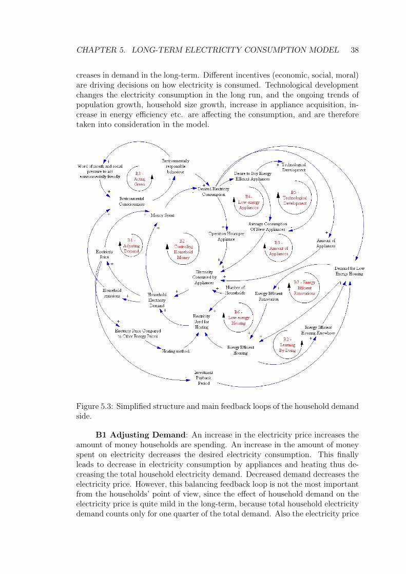
CHAPTER 5. LONG-TERM ELECTRICITY CONSUMPTION MODEL 38
creases in demand in the long-term. Different incentives (economic, social, moral)are driving decisions on how electricity is consumed. Technological developmentchanges the electricity consumption in the long run, and the ongoing trends ofpopulation growth, household size growth, increase in appliance acquisition, in-crease in energy efficiency etc. are affecting the consumption, and are thereforetaken into consideration in the model.
Figure 5.3: Simplified structure and main feedback loops of the household demandside.
B1 Adjusting Demand: An increase in the electricity price increases theamount of money households are spending. An increase in the amount of moneyspent on electricity decreases the desired electricity consumption. This finallyleads to decrease in electricity consumption by appliances and heating thus de-creasing the total household electricity demand. Decreased demand decreases theelectricity price. However, this balancing feedback loop is not the most importantfrom the households’ point of view, since the effect of household demand on theelectricity price is quite mild in the long-term, because total household electricitydemand counts only for one quarter of the total demand. Also the electricity price

CHAPTER 5. LONG-TERM ELECTRICITY CONSUMPTION MODEL 39
is roughly one-third of the total bill due to the transfer costs and taxes.B2 Controlling household money: This is almost the same loop as
B1. Increase in the amount of money spent on electricity decreases the desiredelectricity consumption. This finally leads to decrease in electricity consumptionby appliances and heating thus decreasing the total household electricity demand.Decreased demand decreases the amount of money spent on electricity. Comparedto the loop B1 this is much more relevant; decisions are affecting the amount ofmoney spent directly. This loop can also be seen as willingness to shift opera-tion time of appliances. This is possible if new tariff structures are introduced.However, shifting the appliance time of use does not change the overall electricityconsumption.
B3 Amount of Appliances: This is partly the same as B1 and B2. De-crease in desired electricity consumption decreases the amount of appliances pur-chased, which decreases the household electricity consumption.
B4 Low-energy Appliances: Decrease in desired electricity consumptionincreases the desire to buy energy efficient appliances, which leads to decrease inhousehold electricity consumption.
B5 Technological Development: Technological development describeshow the demand for energy efficient appliances increases the investments in newenergy efficient technologies.
B6 Low-energy Housing: Increase in desired electricity consumption in-creases the demand for low energy housing, which increases the building of newenergy efficient housing. Energy efficiency in housing is also affected by consumerdemand, which depends on household money used for electricity.
B7 Energy Efficient Renovations: This is part of the loop B6. Increasesin the demand for low energy housing increase the amount of energy efficientrenovation people are willing to do. This leads to increase in energy efficienthousing, which will eventually decrease the electricity consumption.
R1 Acting Green: This describes the reinforcing loop in how environ-mental consciousness increases the environmentally responsible behavior, whichfurthermore affects the word of mouth and social pressure, thus increasing theenvironmental consciousness. This can lead to exponential growth or collapse inenvironmentally responsible behavior. This feedback loop is excluded from the fi-nal model due to the difficulty of modeling and lack of data. However, already bystudying the causal loop diagram interesting scenarios can be seen. If householdemissions are reduced significantly, for example due to an increase in renewableenergy production, the incentive for environmental consciousness is decreased,and therefore a vicious cycle is possible in the loop, resulting in a collapse inenvironmentally responsible behavior.
R2 Learning by Doing: Increase in energy efficient housing decreases thecosts of building a low energy house and a low-energy renovation. This loop isexcluded from the model due to lack of data.
Conclusion: Energy consumption in households is an interesting process.Most of the feedback loops described are not likely to affect the electricity con-sumption greatly, although they have some effect, especially in the long-term. In

CHAPTER 5. LONG-TERM ELECTRICITY CONSUMPTION MODEL 40
some cases, e.g. a one-room flat, households consume relatively small amounts ofelectricity, and possible savings due to behavioral changes are minimal. Therefore,in some cases environmental incentives might have a greater impact than economicincentives. For better simulation results, the model could be segmented to coverdifferent consumer segments, e.g. price-conscious and ecologically-conscious con-sumers. Also heating method segments and household type segments could beused to determine more accurately what the benefits of saving electricity are,since an electrically heated detached house has more incentives to save electricitythan a district heated one-room flat.
It is not likely that the behavior of small apartment houses will changesubstantially, especially if district heating is used. At least money will not bethe main motive to use less electricity in these cases. Increasing environmentalconsciousness might have a larger impact on consumers who cannot save money.
5.3 Detailed Description of the Model
In this section, the structure of the model is explained in detail using stock and flowdiagrams. The model is divided into seven submodels: dwelling stock, appliancestock, desire to conserve electricity, electric vehicles, supply side, propagation ofsmart meters and the effect of information, and environmental consciousness.Simplified stock and flow diagrams are presented here, for the original diagramssee Appendix B.
5.3.1 Dwelling Stock
The dwelling stock and the energy consumption of dwellings is modeled usingaging-chain [1, p.470] and co-flow structures [1, p.479]. Aging-chain describes theaging process of the dwelling stock, Figure 5.5, whereas co-flow catches the energyconsumption of these dwellings, Figure 5.7.
Figure 5.4 presents a causal loop diagram of the dwelling stock and Figure 5.5describes the stock and flow diagram of the dwellings.
Figure 5.4: Causal loop diagram of the dwelling stock.

CHAPTER 5. LONG-TERM ELECTRICITY CONSUMPTION MODEL 41
Dwelling stock is described by a series of first order delays. Three firstorder delays form an aging chain of third order delay, as seen in Figure 5.5.Constructing the model this way enables to keep track on the amount of dwellings,which are divided into detached, row, and apartment houses. All these groups arefurthermore divided based on the heating method, which are divided into electric,districts, oil, biomass heating, and ground source heat pumps (GSHP). Electricheating could further be divided into direct and storage heating.
Figure 5.5: Aging-chain of the dwelling stock.
When a new dwelling is constructed, it enters a dwelling stock, which is de-scribed by an inflow Construction of Dwellings. The dwelling stays in the dwellingstock, New Dwellings, Used Dwellings, and Old Dwellings until it is demolished.Demolition is described by an outflow Demolition of Old Dwellings. The averagelifetime of a building describes how long a dwelling is in the dwelling stock on av-erage. The lifetime distribution and cumulative lifetime distribution of a dwellingstock is given in Figure 5.6. The figure shows how the demolition/renovation of10 000 houses constructed in 1990 is distributed given that the average life/reno-vation time is 50 years. The inertia of the dwelling stock has been analysed morecarefully in the work of Pruyt et al. [45].
(a) Lifetime distribution (b) Cumulative lifetime distribution
Figure 5.6: How demolition or renovation of 10 000 houses constructed in 1990 aredistributed given that the average life/renovation time is 50 years. X-axis showsthe year and y-axis denotes number of dwellings.

CHAPTER 5. LONG-TERM ELECTRICITY CONSUMPTION MODEL 42
Figure 5.7 presents how the energy consumption of dwellings is modeledusing aging-chain and co-flow structures. When a dwelling is constructed, theheating it consumes is stored to another aging-chain and when a dwelling is de-molished, the heating it consumes is removed from the heating stock. This allowstaking into account that older dwellings consume more energy than newer ones.The heating consumption of a dwelling depends on the average energy consump-tion per m2 and the average floor area. Both energy consumption and floor areaare changing over time.
Figure 5.7: Dwelling stock and electricity consumed by dwellings.
In the model renovations and demolitions are not distinguished. The energyconsumption is under interest, and therefore it does not matter if the dwelling isdemolished and a new dwelling is built or if the dwelling is renovated using newregulations. Renovated dwellings are not as good as new ones, and therefore aparameter is added to compensate this flaw. The model is working and it is keptas simple as possible. Nevertheless, more accurate results could be achieved byseparating demolitions and renovations.
The average lifetime of 50 years is used in the model. This is a roughestimate, because data on the average lifetime is scarcely available and demolitionsand renovations are not distinguished. This parameter can be changed by themodel user.
5.3.2 Appliance Stock
The appliance stock, seen in Figure 5.8, is modeled in the same way as the dwellingstock, using aging-chains and co-flows. When appliances are purchased, theyenter the New Devices -stock. After one third of the average lifetime has passed,

CHAPTER 5. LONG-TERM ELECTRICITY CONSUMPTION MODEL 43
they enter Used Devices -stock. Again after one third of the average lifetimethey enter Old Devices -stock. Finally after one third of the average lifetime theappliances are recycled. This is a third order system by which it is possible tomodel how long an appliance is in the appliance stock on average. When theconsumer purchases an appliance now, it will take on average X years before anew appliance is purchased, even if a new low energy appliance is introducedjust after the purchase. The average lifetimes of appliances are introduced in theAdado report [46].
Figure 5.8: Appliance stock and appliance stock electricity consumption.
Appliances are currently divided into different subgroups, e.g. lighting, carheating, sauna, HVAC (heating, ventilation, and air conditioning), entertainment,laundry, cooking, refrigeration, and floor heating; every appliance group is mod-eled separately with different parameters. Figure 5.9 presents how the lifetimes ofdifferent appliances affect the lifetime distribution, lighting and dishwashing aretaken as examples. The lifetime of an incandescent bulb is assumed to be twoyears and the lifetime of a dishwasher 12 years.

CHAPTER 5. LONG-TERM ELECTRICITY CONSUMPTION MODEL 44
(a) Lifetime distribution (b) Cumulative lifetime distribution
Figure 5.9: The plots show how recycling of 10 000 appliances purchased in 1990are distributed given that the average lifetime for lighting devices is two years andtwelve years for dishwashers.
5.3.3 Desire to Conserve Electricity
Consumber behavior is an ambiguous but important phenomenon to model. Fig-ure 5.10 presents how desire to conserve electricity is modeled.
Desire to conserve electricity affects how willing people are to purchase en-ergy efficient appliances and low energy housing. Therefore it is an interestingand important variable, which is very difficult to model. The desire to conserveelectricity is modeled using several variables, in the model it depends on Elec-tricity bill relative to income, Effect of information, Environmentally responsiblebehavior, and Experienced Value of Electricity.
When consumers have more information available on their consumption,they can change their consumption habits. Consumers also react to the changesin the electricity price, but currently electricity price for households does not varymuch. This could change if new tariff structures was introduced.
Figure 5.10: Desire to conserve electricity.

CHAPTER 5. LONG-TERM ELECTRICITY CONSUMPTION MODEL 45
Eq. (5.1) presents how Desire to Conserve Electricity is modeled, a multi-plicative formulation is used. Electricity Bill Relative to Income, Effect of Infor-mation, Environmentally Responsible Behavior, and Experienced Value of Elec-tricity are thought independent of each other, however, the combined effects ofthese factors depend on each other. For instance, if one has information abouthow to conserve electricity and environmental incentives, but lacks money, thenthat affects the strength of the overall effect multiplicatively.
DtCE = EBRtI × EoI × ERB × EV oE (5.1)
The exponents Elasticity of DfEEA (EoDfEEA) and Elasticity of DfEEH(EoDfEEH) determine how strong the effect of Desire to Conserve Electricity(DtCE) is on the Demand for Energy Efficient Appliances (DfEEA) and Demandfor Energy Efficient Housing (DfEEH) respectively, see Eqs. (5.2) and (5.3).
The exponents can be estimated in the following way. To represent a 50%increase in Demand for Energy Efficient Appliances (DfEEA) when the Desire toConserve Electricity (DtCE) doubles, set EoDfEEA = log2(1.5) ≈ 0.58. For a10% increase for Demand for Energy Efficient Housing (DfEEH) when the Desireto Conserve Electricity (DtCE) doubles set EoDfEEH = log2(1.1) ≈ 0.14. Fora more detailed mathematical explanation see [1, p.338 and p.507].
DfEEA = DtCEEoDfEEA (5.2)
DfEEH = DtCEEoDfEEH (5.3)
Eqs. (5.4) and (5.5) present the formulas for Demand for Appliances (DfA)and Demand for Housing (DfH). Using the same analogy as previously the ex-ponents for appliance and housing demand can be estimated. To represent a 7%decrease in Demand for Appliances (DfA) when the Desire to Conserve Electricity(DtCE) doubles, set EoDfA = log2(0.93) ≈ −0.10. For a 4% decrease for De-mand for Housing (DfH) when the Desire to Conserve Electricity (DtCE) doublesset EoDfH = log2(0.96) ≈ −0.06.
DfA = DtCEEoDfA (5.4)
DfH = DtCEEoDfH (5.5)
5.3.4 Supply side: Price, Capacity and Production.
The supply side is kept relatively simple as the main focus is on the demand side.Vogstad [36] has modeled electricity production in the Nordic electricity marketsquite comprehensively in his study. Vogstad’s model has been used as a startingpoint of the supply side submodel. Electricity production is not the main topicin this study, but it is important to include some of the feedback loops fromthe production side to the model. The electricity price affects both demand and

CHAPTER 5. LONG-TERM ELECTRICITY CONSUMPTION MODEL 46
production in the long-term, and therefore the effect of the price to the capacityand the capacity to the price has been modeled here. Figure 5.11 presents thesubmodel of the electricity supply side.
Figure 5.11: Capacity and production.
Important dynamics affecting the system in the long-term comes from theconstruction of new capacity. As seen in the model, when new capacity is decidedto be built, it enters the Capacity under Construction stock, and after the av-erage construction time it enters the Capacity stock. Construction delay can besomething between two and ten years depending on the project. The new nuclearpower plant decision, for instance, already came in 2001, and the plant is stillunder construction, with the estimated completion time at the moment being in2014 [47]. This is a major feedback loop with significant delay, thus producingoscillation to the capacity and price.
Simulations revealed that the feedback from household consumption to the

CHAPTER 5. LONG-TERM ELECTRICITY CONSUMPTION MODEL 47
electricity price is relatively mild, and therefore, for the sake of simplicity, thesupply side is excluded from the model analysis. Instead, a simple exponentialgrowth model is used, see Figure 5.12. However, it is worth mentioning that thisdoes not mean that the household consumption is not affecting the electricityprice. The model lacks the feedback loop from the short-term model, i.e. fromload profiles, to the long-term model. Even though household consumption isroughly a quarter of the total consumption of Finland, the impact on the priceis probably more significant, because of peak demand. The model is not capableof taking into consideration the effect of load profiles to the electricity price; thisrequires further research.
Figure 5.12: Electricity price.
5.3.5 Hybrid and Electric Vehicles
Figure 5.13 presents the submodel describing hybrid and electric vechichle (HEV)electricity consumption. This submodel is created because of the huge impactHEVs can have on the electrical grid in the long run. This is also an exampleof how different submodels can be added to the model without a feedback loopfrom other parts of the model. This could also be replaced by existing scenarios,but including this enables testing how the total consumption will change withdifferent assumptions together with other parts of the model.
Two parameters are given to the model user, the starting year of HEV boomand the contact rate, which describes how fast HEVs will become dominant. Themodel is fit to follow the base scenario given by Ruska et al. [14]. The model is amodification of a Bass diffusion model [48] [1, pp.332-347] and research of Strubenand Sterman [49] is used as a reference. This is a simplified model and the wordof mouth is used as the dominant propagation cause; vehicle features, advertising,subsidies etc. are excluded.
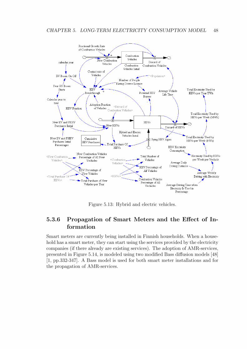
CHAPTER 5. LONG-TERM ELECTRICITY CONSUMPTION MODEL 48
Figure 5.13: Hybrid and electric vehicles.
5.3.6 Propagation of Smart Meters and the Effect of In-formation
Smart meters are currently being installed in Finnish households. When a house-hold has a smart meter, they can start using the services provided by the electricitycompanies (if there already are existing services). The adoption of AMR-services,presented in Figure 5.14, is modeled using two modified Bass diffusion models [48][1, pp.332-347]. A Bass model is used for both smart meter installations and forthe propagation of AMR-services.

CHAPTER 5. LONG-TERM ELECTRICITY CONSUMPTION MODEL 49
Figure 5.14: Smart meter and AMR-service propagation.
In a normal Bass model all adopters are spreading the word of mouth, butit is more likely in this case that after the purchase of a new service people spreadthe word a certain time and after a while their enthusiasm decreases and they areno longer spreading the word. This can be modeled by dividing adopters into twostocks, new adopters and former adopters. New adopters have just purchased thenew service and they are spreading the word. Former adopters have purchasedthe service a while a go and they are no longer that excited about it.
Eq. (5.6) presents the formula for Information How Much Energy Can BeSaved (IHMECBS), which depents on Percent of Households Utilizing AMR (Po-HUAMR) and Elasticity of AMR Information (EoAMRI). The exponent Elastic-ity of AMR Information (EoAMRI) determines how strong the effect of Infor-mation How Much Energy Can Be Saved (IHMECBS) is. This can be estimatedin the same way as in the desire to conserve electricity. To represent 15% in-crease in Information How Much Energy Can Be Saved (IHMECBS) when the1 + PoHUAMR doubles, set EoAMRI = log2(1.15) ≈ 0.20.
IHMECBS = (1 + PoHUAMR)EoAMRI (5.6)
In this model, an assumption is made that information has permanent effect

CHAPTER 5. LONG-TERM ELECTRICITY CONSUMPTION MODEL 50
on people’s behavior. However, this is not necessarily true, Pihala [50] emphasizesthat current studies have not yet confirmed this, hence future research is required.
5.3.7 Environmental Consciousness
Environmental consciousness is an interesting variable in the model. It affects thesystem in the long-term. Modeling environmental consciousness is not an easytask, nevertheless it is taken into account in some sense in the model as a scenariovariable. The user can determine the growth rate of environmentally responsiblebehavior.
Figure 5.15 presents a sketch of the submodel describing environmental con-sciousness. This submodel is not included in the model, because the detailedmodel is not seen as important as other parts of the model and the model is keptas simple as possible. Nevertheless, this can be added to the model if needed.
Figure 5.15: Environmental consciousness and acting green.
In Figure 5.15 environmental consciousness is divided into two variables,environmental consciousness and environmentally responsible behaviour, becausepeople’s consciousness can increase without them acting accordingly. Environ-mental consciousness is gained through education and time; this is a slow process.Environmentally responsible behaviour also depends on people’s wealth. If peopledo not have money, they might not act environmentally consciously.

CHAPTER 5. LONG-TERM ELECTRICITY CONSUMPTION MODEL 51
In this model, environmentally responsible behaviour affects both the deci-sion whether to buy new appliances and the energy efficiency of the purchasedappliances.
5.4 Testing and Validation
It should always kept in mind that all models are wrong or inadequate, althoughsome models can be useful. In this chapter model assumptions are tested andflaws are tried to discover. The model is validated against historical data, and acomprehensive list of the validation results can be seen in Appendix A.
The model has been discussed with other researchers and the structure hasbeen adjusted when flaws have been observed. The validation methods presentedin Chapter 3 have been used in model validation throughout the modeling process.
Even if the model is capable of following historical data the model correctnessis not yet proven. There is a possibility that the model explains the history withoutcatching the process behind the data. If the model is not ”predicting” the history,then the assumptions must be adjusted according to available information or themodel should be rejected. It is important to understand that fitting the modelto follow historical data does not mean that the model is correct. It only meansthat we cannot reject the model based on historical data, since history data onlyreveals one possible path among others. This is why other validation methods areneeded.
A large amount of historical data is used in the model validation. The datahas been collected mostly from the literature and from Statistics Finland (Tilas-tokeskus). Dwelling stock and the changes in the dwelling stock have been fittedusing the studies by Pesola et al. [51] and by Lehtinen et al. [52]. Dwellingenergy consumption has been derived from a study of Laitinen [53]. Data fromStatistics Finland has been used in many parts of the model. Most useful reportshave been the following: Asunnot ja asuinolot 2010 [54], Rakennus ja asunnon-tuotanto 2011 [55], Korjausrakentaminen 2010 [56], Vaestoennuste 2009-2060 [57],and Ajankayttotutkimus 2009 [58]. A report by Koreneff et al. [59] has been usedto fit the overall consumption of households, industry, and services. Householdappliance energy consumption data has been gathered from different sources, themost useful have been Adado [46] and Korhonen et al. [60]. Household lightingscenarios have been derived from a study of Sarvaranta [61] and Korhonen et al.[60]. Data on electricity prices, production, and capacity have been gathered fromNord Pool official website [6] and from the Finnish Energy Market Authority [4].Data on the propagation of ground source heat pumps has been derived fromFinnish heat pump association (Sulpu ry) [62] and data on the efficiency of heatpumps has been derived from [62] and [20].
5.4.1 Validation Simulations
The following figures present validation results against historical data. Data hasbeen gathered from literature, as described earlier, and validation has been done

CHAPTER 5. LONG-TERM ELECTRICITY CONSUMPTION MODEL 52
against all found data. The behavior of several other variables have also beenvalidated against historical data, for example: the percentage of households hav-ing different appliances, total electricity consumed by different appliance groups,number of dwellings, dwelling electricity consumption, average floor areas, GSHPpurchases etc.
Figure 5.16 presents how households are divided between building types.Historical data is from Statistics Finland [54].
Figure 5.16: Number of households per building type: Detached houses, rowhouses, and apartmets.
Figure 5.17 presents the electricity consumption for laundry. Historical datais from the Adato-report [46].
Figure 5.17: Average electricity consumption for laundry.

CHAPTER 5. LONG-TERM ELECTRICITY CONSUMPTION MODEL 53
Figure 5.18 presents the GSHP installations given by the model. Historicaldata is from Sulpu [62].
Figure 5.18: GSHP installations. Historical data from Sulpu Ry [62].
5.4.2 Sensitivity Simulations and Variable Analysis
With sensitivity simulations, the model robustness to parameter changes can bestudied. Also several variables are examined more carefully. In sensitivity simu-lations, the results are shown with confidence intervals, e.g. 50%, 75%, 95%, and100% of the trajectories being inside the shown area.
Effect of Price:Figure 5.19 presents how varying the electricity price growth rate between
0 and 4% changes the electricity price. The growth rates presented in this thesisare always thought as real growth rates. The annual income growth rate is set atzero. The initial electricity price is set to 20e/MWh. With 4% growth rate, theprice will be 216e/MWh in 2050, which means more than a tenfold increase.

CHAPTER 5. LONG-TERM ELECTRICITY CONSUMPTION MODEL 54
Figure 5.19: Sensitivity analysis: Electricity price (electricity price growth rate isvaried between 0 and 4% per year).
As can be seen from Figure 5.20, the average money spent on electricityincreases at maximum from 800eto 1700e, which is approximately a twofoldincrease. Also the electricity bill relative to income, Figure 5.21, is increasing atmaximum twofold.
Figure 5.20: Sensitivity analysis: Money spent to electricity (electricity pricegrowth rate is varied between 0 and 4% per year).

CHAPTER 5. LONG-TERM ELECTRICITY CONSUMPTION MODEL 55
Figure 5.21: Sensitivity analysis: Electricity bill relative to income (electricityprice growth rate is varied between 0 and 4% per year).
Figure 5.22 and Figure 5.23 present the effect of the varied electricity price onappliance and heating consumption respectively. As can be seen from the figures,there is roughly 10% difference in both appliance and heating consumptions.
Figure 5.22: Sensitivity analysis: Household appliance electricity consumption(electricity price growth rate is varied between 0 and 4% per year).

CHAPTER 5. LONG-TERM ELECTRICITY CONSUMPTION MODEL 56
Figure 5.23: Sensitivity analysis: Household heating electricity consumption (elec-tricity price growth rate is varied between 0 and 4% per year).
Heating methods:There are several variables that clearly affect the household consumption
more than others. For instance, ground source heat pumps have significant ef-fect on heating electricity consumption. Figure 5.24 presents the future trendsin detached house heating methods with a reference scenario by Laitinen [53].Figure 5.25 presents the GSHP propagation scenario predicted by the model.
Figure 5.24: Detached house heating method proportions: electric, oil, district,biomass, and GSHP heating.

CHAPTER 5. LONG-TERM ELECTRICITY CONSUMPTION MODEL 57
Figure 5.25: GSHP installations and historical values from Sulpu Ry [62].
As seen from the figures, the GSHP installations will change the heatingmethod proportions. The propagation of GSHPs has a significant effect on heat-ing electricity consumption, since GSHPs are replacing direct electric heating inhouseholds, thus the electricity consumption is decreased; The Enete-project [20]suggests that the true annual savings of GSHP are between 27% and 47%. Thisis one of the main reasons why household heating electricity consumption startsto decrease, and the turning point will be seen between 2012-2015.
Sensitivity analysis Figure 5.26 reveals how varying the annual savings ofGSHPs electricity consumption between 25% and 47% affects the aggregated elec-tricity consumption of households given that the GSHPs propagate as seen inFigure 5.25.
Figure 5.26: Sensitivity analysis: GSHP efficiency effect on electricity consump-tion.

CHAPTER 5. LONG-TERM ELECTRICITY CONSUMPTION MODEL 58
Figures 5.27 and 5.28 present results related to Figure 5.26 with additionalsensitivity simulations. Now also the adoption fractions of GSHPs, which describethe propagation rate, are varied, see Table 5.2. Lower adoption fractions are usedto represent the effect of slower propagation; original values are the same themaximum values in the table. As seen in Figure 5.27, varying adoption fractionsdoes not have significant effect on GSHPs propagation in long-term. As seen inFigure 5.28, in short-term, varying adoption fractions have minor effect on GSHPannual energy savings and in long-term the savings are not increasing. This isa result of the systems structure; even though the propagation starts slower, thepositive feedback loop dominates the process and GSHP will eventually overtakethe market of direct electric heating.
Table 5.2: GSHP adption fraction sensitivity parameters.
Parameter Min Max
GSHP adoption fraction (Detached house) 20 26GSHP adoption fraction (Row house) 18 24
Figure 5.27: Sensitivity analysis: GSHP adoption fraction effect on GSHP instal-lations.

CHAPTER 5. LONG-TERM ELECTRICITY CONSUMPTION MODEL 59
Figure 5.28: Sensitivity analysis: GSHP adoption fraction effect on electricityconsumption.
5.5 Scenarios and Using the Model
In this section two different scenarios are discussed. First a base scenario ispresented, which is fitted to follow scenarios found in the literature. Next asecond scenario is presented with different assumptions, and then compared tothe base scenario.
5.5.1 Base Scenario
Figure 5.29 presents simulation results. A reference case is derived from a reportby the Ministry of the Environment [63]. The base scenario is a business asusual, BAU, case, where the ongoing trends of population growth, construction,and income are assumed to continue. Scenario S1 is generated using the mostlikely parameter values , e.g. energy saving policies, and it is fitted to roughlyfollow the reference scenario. Scenario S2 is the alternative scenario with differentparameters; in this case the parameters are chosen to neglect most of the energysaving measures. Table 5.4 presents the altered parameter values. HEVs possibleelectricity consumption is also presented in the figure. The HEV scenario is fittedto roughly follow the scenario presented by Ruska et al. [14].

CHAPTER 5. LONG-TERM ELECTRICITY CONSUMPTION MODEL 60
Table 5.4: Parameter values of scenarios S1 and S2.
Parameter S1 S2 Unit Explanation
Technology AdoptionRate
0.008 0.005 Appliance technologiacal develop-ment rate factor
Energy Policy 2012 10 0.0 % Dwelling energy policy: decrease %Energy Policy 2020 10 0.0 % Dwelling energy policy: decrease %Energy Policy 2030 10 0.0 % Dwelling energy policy: decrease %Energy Policy 2040 10 0.0 % Dwelling energy policy: decrease %GSHP Efficiency 60 70 % GSHP energy consumption com-
pared to direct electric heating
Energy policy 2012, 2020, 2030, 2040 are parameters, which the scenarioanalysis tool user can alter. They describe the dwelling energy consumption de-creases. GSHP Efficeincy describes how much energy GSHP consumes on averagecompared to direct electric heating.
The difference between S1 and S2 is significant in 2050. S1: Appliances:15.92 TWh, Heating: 8.08 TWh, and total: 24.00 TWh. S2: Appliances: 19.68TWh, Heating: 10.77 TWh, and total: 30.45 TWh. Total difference is 6.45 TWh,which is roughly 7% of current electricity consumption. For comparison: theannual electricity generation of nuclear power units Olkiluoto 1 and 2 is roughly 7TWh [47]. However, it should be kept in mind that scenarios ranging to 40 yearsahead should be treated with caution.
Scenario S1 has a clear turning point in heating consumption in 2012; aturning point can also be seen in scenario S2, but the effect is not as strong.Occurrence of the turning point is due to the GSHP fast propagations which hasalready taken place, as discussed earlier, together with energy saving policies inthe heating consumption of new dwellings. The turning point in the reference caseis later, in 2020, than the model suggests. In scenario S2 the average efficiency ofGSHP is assumed to be slightly lower than in S1; S2 also lacks other energy savingmeasures. In scenario S1 an assumption of 10% energy savings to new dwellingsevery decade is used. The long-term effect is significant, resulting in 2.69 TWhsavings in 2050.
Appliance consumption scenarios are more difficult to generate. The differ-ence in the scenarios is a result of the different technology adoption rate. In S1 theenergy consumption of appliances is decreasing faster than in S2. The applianceconsumption given by the scenarios stays almost the same until the year 2025,and after that the consumption starts to diverge rapidly.

CHAPTER 5. LONG-TERM ELECTRICITY CONSUMPTION MODEL 61
Figure 5.29: Total consumption of households: Scenarios 1, 2, and a referencecase.
5.5.2 Other Scenarios
The scenario analysis tool user can test his/her own assumptions and comparethem to the base scenario. Scenarios made in the model should always be com-pared to the base scenario and not thought as forecasts.
5.5.3 Propagation of Appliances
Figure 5.30 presents how fast new technologies, e.g. the smart grid enabled tech-nologies, can emerge in the very best case. Figure 5.30a presents the case ofdishwashers and Figure 5.30b the case of HVAC-devices. In the maximum speedof propagation an assumption is made that all purchased appliances from a givenmoment are new technology appliances. In practice this is of course not the case,new technologies are emerging relatively slow in the beginning due to several rea-sons. For example, before new services for these new technologies are commonthey are not likely to propagate rapidly. The effect of circulation speed is veryobvious here, as the average life time for a dishwasher is 12 years and for a HVAC-

CHAPTER 5. LONG-TERM ELECTRICITY CONSUMPTION MODEL 62
device 30 years. If a new technology is introduced now for all new HVAC-devices,it takes 13 years (not 15 years because of the HVAC-device -stock growth) before50% of the HVAC-device -stock has the new technology. In reality the propaga-tion of a new technology starts slowly, increases, and then saturates. This affects,for instance, the propagation of smart grid enabled solutions, e.g. the demandresponse.
(a) Dishwashing maximum speed of circula-tion
(b) HVAC (heating, ventilation, and air con-ditioning) maximum speed of circulation
Figure 5.30: Speed of circulation describes how fast new smart grid enabled tech-nologies can emerge. The x-axis presents years and the y-axis proportions of allparticular appliances.
5.6 Future Research
The model could be further developed, for instance, the electricity price is notcompared to other energy sources, which limits the usage of the model. If theelectricity price is increasing compared to other energy sources, e.g. oil or biomass,then electric heating would lose market share to other heating methods and viceversa.
Summer houses are left outside of the study, because it is assumed that theydo not have a significant effect on the total electricity consumption. However,more research is needed and if required, they can be taken into consideration inthe model.

Chapter 6
Short-term ElectricityConsumption Model
This chapter presents the short-term model built in this thesis. Section 6.1 ex-plains why the model is created and gives a short description of earlier researchin this topic. Section 6.2 explains the structure of the model. Section 6.3 presentsdetailed description of the short-term model. Section 6.4 presents the ideas be-hind appliance usage probabilities. Section 6.5 explaines how the parameters aregenerated for different households. Section 6.6 explains the testing and validationof the model. Section 6.7 presents the simulation results. Section 6.8 discussesthe development ideas of the model.
6.1 Introduction
The short-term household electricity model made in this thesis is a bottom-upapproach describing how aggregated household appliance electricity consumptionemerges. The short-term model is needed for load profile generation and to testthe integrated model introduced in Chapter 7. The model is built using Aprosmodeling environment [64] and Microsoft Excel.
The model is composed of an Apros-model describing the appliances of asingle household, to be used together with Excel. The model is simulated severaltimes with different parameters in order to obtain the load profiles. The simulationhorizon of the model is one year, and the time resolution is 15 minutes. Thereforethe model is capable of generating daily, weekly, monthly, and annual load profiles.The model does not describe long-term change in electricity consumption.
Household electricity consumption can be divided into household appliancesand heating (and cooling) devices. This short-term model concentrates on districtheated households, therefore excluding electric heating. The electricity consump-tion of appliances is divided into smaller segments, e.g. lighting, cooking, enter-tainment. The main idea is that if inhabitant is at home then appliances can beused. If no one is at home, then appliances are not used, except appliances thatare on all the time, e.g. refrigeration devices. For every hour of the day probabil-ities are predefined for inhabitants being at home and for appliances being used.
63

CHAPTER 6. SHORT-TERM ELECTRICITY CONSUMPTION MODEL 64
Parameters are drawn from predetermined probability distributions.Similar bottom-up approaches are found in the literature. Richardson et al.
[65] have chosen a very similar approach for his model. Although even higher timeresolution are advocated, i.e. 1 minute; the 15-minute time interval is chosen forthis model. Richardson et al. have also seen the need to introduce daily proba-bility profiles for every appliance group although the probabilities are determinedslightly differently. Also Paatero et al. [66], Capasso et al. [67], Seppala [39],Armstrong et al. [68], and Widen et al. [69] have done similar models.
In this thesis, the household electricity consumption model is used as a toolfor illustrating the method of using top-down and bottom-up simulation modelstogether. The calibration and validation of this short-term model is left for futureresearch although calibration and validation methods are discussed.
Earlier research has usually concentrated on simulating current load profiles.However, the purpose of this model is to generate future load profiles. The modelcan be used alone to generate current load profiles, but the true benefit is gainedwhen integrated into the long-term model, which enables simulating the evolutionof load profiles over time.
A large amount of AMR-data is available for the model calibration andvalidation, and this has also affected the structure of the model. The calibrationand validation process is difficult, and therefore it is wise to make it as easyas possible. This model differs from the other similar models because of thepossibility to validate the model against the true statistical properties of householdelectricity consumption.
6.2 Structure of the Model
Figure 6.1 presents the general idea how the appliance electricity consumption ismodeled. Apros-model describes a general household and it can be adjusted todescribe any household using different parameters. Simulating a single householdseveral times gives the advantage of studying the behavior of a single householdand the aggregated effect of several households.
Figure 6.1: General description of the short-term model.

CHAPTER 6. SHORT-TERM ELECTRICITY CONSUMPTION MODEL 65
In the Apros-model time resolution is set to 15 minutes. This enables changesin the consumption at a given hour without increasing the simulation time of themodel to an undesired level.
In Excel, needed distributions are determined. For instance, the householdsize distribution determines household sizes, which are used to determine otherthings in the model, e.g. lighting consumption. This way a comprehensive sampleof households is selected.
6.3 Detailed Description of the Model
The model describes the electricity consumption of household appliances. House-hold appliances are divided into subgroups: lighting, sauna, car heating, entertain-ment, laundry, refrigeration, cooking, floor heating, HVAC (heating, ventilation,and air conditioning), and other appliances. These categories serve the purposeof modeling the change in load profiles and they are also used in the long-termmodel.
The model is composed of the submodels of different appliance groups. Fig-ure 6.2 presents the entertainment appliance submodel. In the model the probabil-ity that an appliance is on comes from the left border. External automation -blockgives out a uniform random variable between 0 and 1. If the random variable isbelow the defined probability, then the appliance is turned on. In the picture therandom variable is 0.2934 and the defined probability is 0.099, which means thatthe appliance is not turned on. If the appliance is turned on, then, in this case,the appliance is running 3600 seconds. This is based on the assumption that anappliance is usually on a given time rather than switching on and off continuouslydependent on the random variable. A laundry machine, for instance, is usuallyon roughly two hours. After deciding if the appliance is on it will be multipliedby House occupants, which is 0 or 1. This means that appliances can be on only ifsomeone is at home. This is of course not the case with refrigeration devices etc.
Figure 6.2: The short-term model - electricity consumption of entertainment ap-pliances.
It is easy to add additional conditions to the model if required. In the car

CHAPTER 6. SHORT-TERM ELECTRICITY CONSUMPTION MODEL 66
heating submodel, for instance, the outdoor temperature is taken into considera-tion. People are using car heating, if the outdoor temperature is below a certaintemperature, e.g. five degrees.
Solar radiation affects the use of lighting devices. In the Nordic countriesthis affects the electricity consumption, since the summer days are long and thewinter days are short and lighting is needed more often.
There are many parameters in the model that can be adjusted, e.g. the powerconsumption of appliances, appliance average operating time at one instance ofuse (when an appliance is turned on, how long it will be used), the probability ofhaving a certain appliance, appliance usage probabilities, etc.
The short-term model, part of it seen in Figure 6.2, describes a single house-hold. In order to obtain load profiles the Apros-model needs to be simulatedseveral times with different parameters. This is done using an Excel user inter-face. VBA-code generates the needed parameters for the simulations from thepredetermined probability distributions, thus giving an extensive set of param-eters. The model describing one household is made using the Apros modelingenvironment, and combined with Excel it describes a large set of households.
6.4 Appliance Usage Probabilities
Electricity consumption has been divided into smaller components, as describedearlier. Appliances can be used when someone is at home. Household occupancyis modeled as a random variable, people are at home or they are not. Householdoccupancy at a certain time of the day follows a given probability distribution.This probability distribution is derived from automatic meter reading (AMR)data. Inhabitants and appliances are separated, because when modeling the fu-ture change in electricity consumption appliance usage probabilities might change,while inhabitant probability of being at home is not likely to change However, ifinhabitant probability of being at home changes, the reasons behind the changeare not the same than behind the change of the appliance usage probabilities. Forexample, if a new tariff structure is introduced, the appliance usage probabilitiesare changing but the probability of being at home is not. Figure 6.3 presents theidea behind the usage of probability distributions.
The probability of being at home is the most important probability distri-bution determined. Probability distributions describing appliance usage probabil-ities are conditional probabilities given that the inhabitant is at home. For everyappliance group a probability distribution is determined, which determines theprobability of turning an appliance on for every hour of the day. Another param-eter defines how long the appliance is on. Weekdays and weekends are treatedseparately.

CHAPTER 6. SHORT-TERM ELECTRICITY CONSUMPTION MODEL 67
Figure 6.3: General description how the short-term model is divided into submod-els.
Conditional probabilities and the Bayes theorem give: Eqs. (6.1), (6.2), and(6.3).
A :=
{1 : Appliance on0 : Appliance off
(6.1)
B :=
{1 : Inhabitant at home0 : Inhabitant not at home
(6.2)
P (A = 1|B = 1) =P (B = 1|A = 1)P (A = 1)
P (B = 1)(6.3)
Using the law of total probability gives: Eq. (6.4)
P (A = 1|B = 1) =P (B = 1|A = 1)P (A = 1)
P (B = |A = 1)P (A = 1) + P (B = 1|A = 0)P (A = 0)(6.4)
P (A) is the probability of using an appliance, i.e. P (A) is the probabilityof using the appliance regardless of anyone being at home. This is difficult tomeasure without test houses. P (A|B) means the conditional probability of usingan appliance given that someone is at home. On the other hand, this is alsodifficult to measure with test households, because it is hard to say if anyone isat home when the appliance is on. However, the conditional probabilities couldbe constructed by experts or by a survey. Separating the probability of beingat home and the appliance probabilities also make it easier to consider differentpopulation groups, because using conditional probabilities it is enough to changeonly the probability of being at home. Also P (A = 1) (appliance is on) is easierto measure than P (A = 1|B = 1) (appliance is on given that someone is athome), since literature already gives estimates of how many hours people areusing different appliances per day and per week.
In most cases P (B = 1|A = 1) = 1, when assumed that a device is off ifno one is at home, although this is not true in all cases. However, this simplifies

CHAPTER 6. SHORT-TERM ELECTRICITY CONSUMPTION MODEL 68
the equation, see Eq. (6.5). This knowledge can be used when determining theprobability distributions.
P (A = 1|B = 1) =P (A = 1)
P (B = 1)(6.5)
The usage probability distributions are presented in the appendix. If thereis nothing that can be said about the shape of the probability distribution, then auniform distribution is used, which means that no information about the particularphenomenon is available.
6.5 Parameter Generation for Different House-
holds
The Apros-model needs to be simulated several times in order to obtain the loadprofiles. As mentioned earlier, every household simulated should be somewhatdifferent. Distributions are used in order to obtain a comprehensive sample ofhouseholds of a different kind. Parameters are obtained by drawing random vari-ables from predetermined probability distributions describing variables. House-hold floor area for a single household, for instance, can be randomly drawn fromhousehold floor area distribution. Furthermore, household equipment level can bedecided based on household floor area, also using distributions.
The same approach can be used to decide whether the household is a de-tached house, a row house, or an apartment and then choose the floor area fromthe floor area distribution. Detached houses are larger than apartments. The sameapproach can be used to determine the number of occupants, the probability ofhaving an appliance, etc.
6.6 Model Calibration and Validation
Model validation is an important part of modeling. As mentioned in previouschapters, a model cannot be proved to be true, because all models are approxima-tions of reality. However, the model can be falsified or its structure and behaviorcan be validated against real data and expert evaluations, and thus conclusionson the usefulness of the model can be made.
There are several ways to test the model. The easiest way is to comparethe simulation results with the results found in the literature. Several studiesgive valuable information on the household electricity consumption. For example,average appliance usage times can easily be compared. Also the simulation resultscan be compared to the load profiles found in the literature. A more sophisticatedmethod is to study the distributions of electricity consumption. This includesstudying the AMR-data. However, a comprehensive validation of the model is notin the scope of this thesis, only validation ideas are presented for future research.

CHAPTER 6. SHORT-TERM ELECTRICITY CONSUMPTION MODEL 69
Data from several studies has been used to calibrate the model, even thoughthe model is not yet ready. The Adato report [46] gives lots of insightful knowledgeabout the household electricity consumption in Finland. The Adato report alsogives information about how the electricity consumption habits have changed,because the same study was made in 1993 and in 2006.
How many hours/days/weeks an appliance is on during a given time is cal-culated in the model and compared to real data. Estimates how long differentappliances are used can be found in [70].
AMR-data is used in the validation of the model. This is possible by usingdistrict heated households chosen from the AMR-data set. District heated house-holds lack electric heating, and therefore their electricity consumption dependsonly on appliances.
6.6.1 Comparison of Existing Load Profiles
The model can be calibrated using existing information on the load profiles. Fig-ure 6.4 presents data how electricity consumption in Swedish households [71] isdivided between appliances and how the load profile arises from this data. Thiskind of data is compared to the data the short-term model is generating, and inthe case of differences calibration is done. The advantage of this approach com-pared to the AMR-data is that this reveals how the load profile is composed ofdifferent appliance load profiles. This rough calibration is a good place to start.
Figure 6.4: Load profile of an apartment: family 26-64 years old, no electricheating, workday. [71]

CHAPTER 6. SHORT-TERM ELECTRICITY CONSUMPTION MODEL 70
6.6.2 Hourly and Annual Electricity Consumption Distri-butions
People consume different amounts of electricity at different times of the day. Whenstudying the consumption of a single household, the consumption might seem quiterandom. However, when studying the statistical properties of the consumption,it can be seen that the consumption is distributed in a well-defined way. Zeroconsumption is rare, but also very large consumption is rare during a single hour.The upper limit of the consumption is the total electricity consumption capacityof one household and lower limit is zero, or in practice it is the standby consump-tion. The statistical properties of electricity consumption can be used in modelcalibration and validation. The simulation results should have the same statisticalproperties as the measured AMR-data has. If AMR-data and the model give dif-ferent distributions or statistical indicators, then we can say that the model is notcorrect and improvements are required. If the model gives the same distributionas the AMR-data, then the model is in this sense correct.
Electricity consumption distributions were presented in Chapter 4, see Fig-ure 4.2. Electricity consumption magnitudes are shown in the x-axis. The fre-quency of how often certain electricity consumption occurred is shown in they-axis.
Some houses consume less energy than others. Household electricity con-sumption distributions are already discussed in Chapter 4. Figure 6.5 presentsreal total household electricity consumption in 2010 (shown in Chapter 4) andthe short-term model output. This can also be used in model calibration in thesame way that the hourly consumption data is used. The model should give asimilar distribution. As seen in the figure, the distributions are clearly different,and therefore improvements are required in the model.
(a) AMR data: household total electricityconsumption. [38]
(b) Apros simulation: household total elec-tricity consumption. X-axis: electricity us-age kWh, y-axis: frequency
Figure 6.5: AMR-data and simulation model distribution comparison.

CHAPTER 6. SHORT-TERM ELECTRICITY CONSUMPTION MODEL 71
6.7 Simulation Results
Figure 6.6 presents a simulation result of a single household. Even though thepattern seen in the figure is quite random, some regularities can already be seen.For instance, the consumption is low during the night and high during the day.Figure 6.7 presents the aggregated effect of several households, now the load profileis emerging and conclusions about the electricity consumption can be made.
To clarify the model structure: the Apros-model gives results like seen inFigure 6.6, as it is a model of a single household. The short-term model, whichis created using the Apros-model and Excel, gives results seen in Figure 6.7, as asingle household is simulated several times and the results are collected in Excel.
Figure 6.6: Simulation of one household.
Figure 6.7: Simulation of several households: load profiles.
More simulation results of the short-term model are shown in the next chap-ter, showing the integration of the short- and long-term models.

CHAPTER 6. SHORT-TERM ELECTRICITY CONSUMPTION MODEL 72
6.8 Further Research
In this thesis, only a framework for the bottom-up electricity consumption modelis implemented. Future research is required to complete the model and to calibrateand validate it.
The model could also be developed by introducing different populationgroups. Probability distribution for being at home could be defined for these pop-ulation groups. Here are some suggestions for how residents could be segmented:nine-to-five workers, shift workers, night workers, senior citizens, unemployed,families with children, students, etc.

Chapter 7
Integration of the Models
The propagation of appliances, heat pumps, entertainment appliances, etc., is acomplex process consisting of interaction of individuals. The shape of load profilesis an aggregated load of all households. However, the propagation of appliancesis changing household consumption, and therefore a link between the consumerbehavior and load profiles is required, which is established in this chapter.
This chapter presents a new approach, which enables simulating the evolu-tion of load profiles over time. Section 7.1 explanes the purpose of the integratedmodel. Section 7.2 presents how the integration is implemented. Section 7.3presents the simulation results. Section 7.4 discusses the future research requiredto be done.
7.1 Purpose of the Integrated Model
Many parties in the electricity markets, e.g. electricity suppliers and distributors,are interested in knowing how electricity load profiles are changing over time.System dynamics gives the long-term trends and the short-term model gives loadprofiles. By combining these two it is possible to simulate scenarios on how theload profiles change over time.
There are two reasons why two models were decided to be created in the firstplace. Use of different modeling techniques allow utilizing the best practises togiven problems and no trade-offs are needed. Of course, if the models were createdusing only one modeling tool, then no integration would be needed. However, themain reason for two different models and integration is the large difference intime constants in the models. The time constant is short in the short-term modeland long in the long-term model, this exposes the model to the problems of stiffsystems. A system is said to be stiff when it has fast and slow dynamics. If thetime constants related to fast and slow dynamics differ significantly from eachother, then the ordinary numerical methods can fail and cause errors. The timestep has to be small enough to capture the fast dynamics, but at the same timeit can be too fast and corrupt the slow dynamics by round-off errors. [1, p.909]
73

CHAPTER 7. INTEGRATION OF THE MODELS 74
7.2 Integration
7.2.1 Models made in this thesis
Table 7.1 presents a summary of the key points of the models created in thisthesis.
Table 7.1: Summary of the models
The Short-term Model The Long-term Model
Bottom-up -approach Top-down -approachTime horizon: one year Time horizon: 40 yearsResolution: hours Resolution: weeksHousehold appliance usage Dynamic long-term phenomenonLoad profiles Change in total electricity consumptionUses data from the long-term model Produces data for the short-term modelValidation against AMR-data Validation against historical dataIndividual households and expert evaluationsand aggregated effects Consumer behavior
Political decision makingScenario analysis tool
7.2.2 Integrated Model Implementation and Usage
Integration is implemented using Microsoft Excel and Visual Basic for Applica-tions (VBA). The created Excel user interface is communicating with both Vensimand Apros programs.
The long-term model is simulated first and then the defined parameters aretransferred to the short-term model, which is simulated using Excel and Apros.In Excel the parameters for the short-term model, i.e. for every household, aredetermined. In Apros the households are simulated with given parameters. Afterthe simulations, the data is imported back to Excel where the results can beprocessed.
7.2.3 Data Transferred Between the Models
The long-term model gives long-term trends, e.g. how the number of households,the number of appliances, energy efficiency, population, and total electricity con-sumption are evolving over time. These variables are transferred into the short-term model.
7.3 Simulation Results
Chapters 5 and 6 already presented the simulation results of the individual models.In this section results of the integrated model are presented.

CHAPTER 7. INTEGRATION OF THE MODELS 75
The total electricity consumption is not the only thing affecting the loadprofiles. Figure 7.1 presents how the relative proportions of appliances change overtime. This affects significantly the load profiles, since appliances have differentpower consumption and are used at different times of the day.
Figure 7.1: Appliances relative to the amount of households.
Figure 7.2 shows how the appliance average power consumptions changesover time. This affects significantly the load profiles. For instance, the lightingpower decrease is one of the major reasons for the change in the load profiles. Theaverage power of appliances describes the energy efficiency of appliances. Otherfactors affecting electricity consumption, such as appliance operation times, aretreated separately.

CHAPTER 7. INTEGRATION OF THE MODELS 76
Figure 7.2: Appliance average power.
The results presented in Figures 7.3, 7.4, and 7.5 are only sketches, since theshort-term model is not yet calibrated. However, preliminary conclusions can bemade and the usefulness of the modeling method can be evaluated.
Figures 7.3 and 7.4 present daily and Figure 7.5 presents weekly load pro-files generated using the integrated model. As explained earlier, first the long-termmodel is simulated and the required variable values from the given time instanceare transferred to the short-term model, which generates the load profiles. Fig-ure 7.6 presents the load profiles derived from AMR-data.
As can be seen in the figures, there is a large difference between the loadprofiles in 1990 and 2050. This is a result of different amounts of appliances andchange in appliance energy efficiency. For instance, in 1990 most of the light-ing devices used are incandescent bulbs whereas in 2050 mostly energy efficientlighting equipments, such as LEDs, are used. This change affects both the totalconsumption and the load profiles. In 1990, the consumption was significantlylower during the night than the day. When investigating the situation in 2050,this has changed, the consumption during the night is still lower than the day, butthe difference is not as large as it was. The major reason for this is the change inlighting equipment energy efficiency, as seen in Figure 7.2.

CHAPTER 7. INTEGRATION OF THE MODELS 77
Figure 7.3: Daily load profiles.
Figure 7.4 presents the same simulation results as seen in Figure 7.3, but nowalso the increased number of households is taken into consideration. In 1990 therewere approximately 2 million households and in 2050 the estimate for householdsis approximately 3.5 million. As can be seen, this changes the situation and theconclusions are not as clear as they were in the previous case; the increase in thenumber of households cancels out the effect of energy efficiency. Figure 7.3 betterdescribes the situation of a city district with no significant change in the numberof households, whereas Figure 7.4 presents the situation in Finland overall, or ingrowing areas.
Figure 7.4: Daily load profiles - corrected with the amount of households.
Figure 7.5 presents the weekly load profiles for the scenarios S1 and S2presented in in Chapter 5.
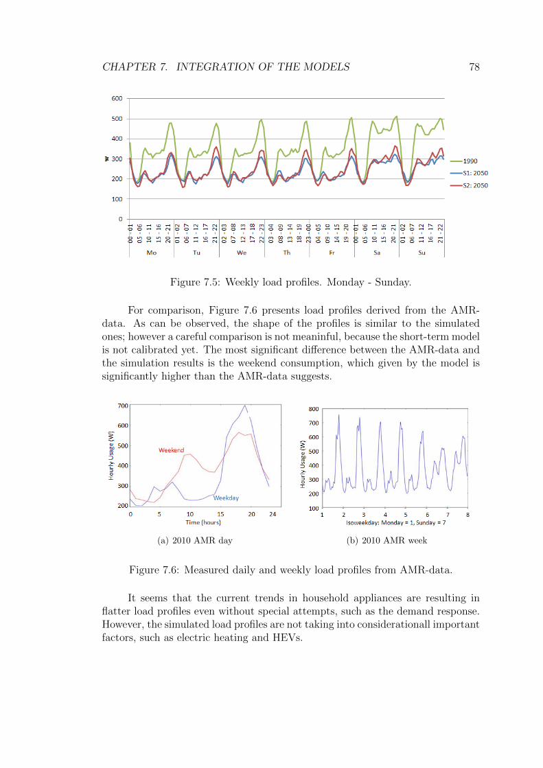
CHAPTER 7. INTEGRATION OF THE MODELS 78
Figure 7.5: Weekly load profiles. Monday - Sunday.
For comparison, Figure 7.6 presents load profiles derived from the AMR-data. As can be observed, the shape of the profiles is similar to the simulatedones; however a careful comparison is not meaninful, because the short-term modelis not calibrated yet. The most significant difference between the AMR-data andthe simulation results is the weekend consumption, which given by the model issignificantly higher than the AMR-data suggests.
(a) 2010 AMR day (b) 2010 AMR week
Figure 7.6: Measured daily and weekly load profiles from AMR-data.
It seems that the current trends in household appliances are resulting inflatter load profiles even without special attempts, such as the demand response.However, the simulated load profiles are not taking into considerationall importantfactors, such as electric heating and HEVs.

CHAPTER 7. INTEGRATION OF THE MODELS 79
7.4 Future Research
The model integration works well although the short-term model is not yet fullyfunctional, and therefore limiting the use of the integrated model.
The integration could be done to work both ways. Now data is transferredonly from the long-term model to the short-term model. The possibility to trans-fer data from the short-term model to the long-term model would enable manyinteresting phenomena, for instance the effect of load profile changes to the elec-tricity production could be studied. In this case it would make sense to includethe supply side submodel again in the long-term model, because flattening loadprofiles affect the hourly electricity price and therefore also the production meth-ods. Flattening load profiles would result in lower demand for load followingpower plants. On the contrary, more volatile load profiles, e.g. due to lack ofload control and load shifting activities, would result in higher demand for loadfollowing power plants instead of base power plants. The bidirectional integrationis possible to implement with the Simantics platform [72].

Chapter 8
Discussion and Conclusion
This chapter states the conclusion and summarises what is done in this thesis. Alsothe scientific contribution to the field of electricity market research is discussed.
Section 8.1 presents the summary and conclusion. Section 8.2 states thescientific contribution of this thesis. Section 8.3 discusses the future researchneeded to be done.
8.1 Summary and Conclusion
The objective was to create a model able to simulate the change of householdload profiles. The used method was a combination of system dynamics and abottom-up modeling method.
The long-term model is capable of reproducing the scenarios found in theliterature, and by changing the assumptions new scenarios can be generated. Thepower of the model lies in the feedback loops, nonlinearities, and delays, whichare difficult to understand for human brains and affect the system behavior sig-nificantly in the long run.
The short-term model is capable of producing household load profiles; how-ever, it is not yet calibrated to reproduce the current measured load profiles,and therefore more research is required. Nevertheless, the model is a structuralbottom-up model, and by adjusting assumptions it can be used for load profiletesting.
The integrated model combines long-term and short-term models. Usingthis entity it is possible to simulate the long-term change in load profiles. This isan important result since it helps understand the reasons behind the change andtest different assumptions. For instance, if it is desired to flatten the load profiles,the effect of different policies can be tested.
The model can also be used to evaluate how different changes affect thebehavior. Residential customers do not see the overall benefits as the electricitymarket utilities see them, and therefore incentives are needed to control householdbehavior. Finding the best way to control household behavior is not trivial. Themodel can be used to evaluate different strategies and help finding variables, whichhave the largest impact in the long run.
80

CHAPTER 8. DISCUSSION AND CONCLUSION 81
The simulation results suggest that the appliance electricity consumptionis going to increase and the dwelling heating electricity consumption is going todecrease. The load profiles are likely to flatten, mostly because of the propagationof energy saving lighting technologies. However, the results are preliminary, andtherefore they should be analysed with caution.
8.2 Scientific Contribution
The developed model is a new approach to load profile modeling. The preliminaryresults and expert evaluations suggest that the approach is useful and it can beused to better understand how load profiles are composed and how decision makerscan influence them.
The model can also be used to evaluate the potential and likely propaga-tion time of demand response methods, since the effect and the adoption time ofdifferent methods can be studied using simulations. This is an important aspectwhen talking about business models concerning the smart grid.
If electricity consumption trends are linked to load profiles in a practicalway, it should be easier to anticipate how different policies are affecting electricitymarkets and household electricity consumption.
8.3 Future Research
Future research has already been discussed at the end of most of the chapters.Here a summary of these future research topics is made.
The model could be enhanced by adding a possibility to introduce new tech-nology to the long-term model, which enables load shifting. The spreading of newtechnology appliances is a dynamic process and the usage time of the old appli-ances has to be taken into account to obtain a general view of the situation. Theload shifting could be taken into account in the short-term model by introducing acontroller which is capable of deciding what time of the day to consume electricitydepending on the electricity price, outside temperature, etc.
Now, the model concentrates only on households, however, the model couldbe developed also to include companies, e.g. offices, shopping centres, and restau-rants. Otherwise the model is not able to represent a whole city, or even a citydistrict.
The modeling platform is also suitable for testing different tariff structures;the short-term model can be developed to take into account the effect of differenttariffs, such as the effect of real-time pricing (RTP) on load profiles in the long-term. This can be used to answer questions like how many households need toadopt RTP-pricing to gain the desired load profile.

References
[1] Sterman, J. D. Business Dynamics: Systems Thinking and Modeling fora Complex World. Mcgraw-hill Education, 2000.
[2] University of Bergen. The System Dynamics Group, What is SystemDynamics, referenced 10.05.2012. http://www.ifi.uib.no/sd/sdinfo.html.
[3] Eurostat. Eurostat price statistics, referenced 11.06.2012. http:
//epp.eurostat.ec.europa.eu/statistics_explained/index.php/Energy_
price_statistics#Further_Eurostat_information.
[4] Energiamarkkinavirasto. Energiamarkkinavirasto: Sahkomarkkinat,referenced 08.11.2011. https://http://www.energiamarkkinavirasto.fi/
alasivu.asp?gid=30&languageid=246.
[5] Borenstein, S. and Bushnell, J. Electricity restructuring: deregulationor reregulation? Technical Report February, University of California EnergyInstitute, 2000. Available at: http://escholarship.org/uc/item/22d2q3fn.
pdf.
[6] Nord Pool. Nord Pool, How does it work, referenced 27.09.2011. http:
//www.nordpoolspot.com/How-does-it-work/.
[7] Viljanen, S., Makkonen, M., Annala, S., and Kuleshov, D. Visionfor European Electricity Markets in 2030. Technical report, LappeenrantaUniversity of Technology, 2011. ISBN 9789522650733.
[8] Giordano, V., Gangale, F., Jrc-ie, G. F., Sanchez, M., Dg, J.,Onyeji, I., Colta, A., Papaioannou, I., Mengolini, A., Alecu, C.,Ojala, T., and Maschio, I. Smart Grid projects in Europe : lessonslearned and current developments. Technical report, European Commission:Joint Research Centre Institute for Energy, 2011. DOI: 10.2790/32946. ISBN9789279204876.
[9] Ford, A. Cycles in competitive electricity markets: a simulation study ofthe western United States. Energy Policy, 27(11):637–658, October 1999.DOI: 10.1016/S0301-4215(99)00050-6. Available at: http://linkinghub.
elsevier.com/retrieve/pii/S0301421599000506. ISSN 03014215.
82

REFERENCES 83
[10] Ford, A. Waiting for the Boom: A Simulation Study for the Power PlantConstruction in California. Energy Policy, 29(11):847–869, 2001.
[11] Amundsen, E. and Bergman, L. Why has the Nordic electricity marketworked so well? Utilities Policy, 14(3):148–157, September 2006. DOI:10.1016/j.jup.2006.01.001. Available at: http://linkinghub.elsevier.com/
retrieve/pii/S0957178706000129. ISSN 09571787.
[12] Fortum. Pohjoismainen sahkomarkkina ja edellakavijyyden evaat, ref-erenced 20.02.2012. http://www.fortum.com/SiteCollectionDocuments/
Corporation/Fortum_sahkomarkkinat_A4_CO.pdf.
[13] Fingrid. Fingrid, referenced 15.11.2011. https://www.fingrid.fi.
[14] Ruska, M., Kiviluoma, J., and Koreneff, G. Sahkoautojen laajankayttoonoton skenaarioita ja vaikutuksia sahkojarjestelmaan. Technical re-port, VTT Technical Research Centre of Finland, 2010. ISBN 9789513874995.
[15] Back, A.-k., Evens, C., Hukki, K., Manner, P., Niska, H., andPykala, M.-l. Consumer acceptability and adoption of Smart Grid. Tech-nical Report 0, SGEM, Helsinki, 2011. ISBN 9789525947083.
[16] Valtioneuvosto. Valtioneuvoston asetus sahkontoimitusten selvityk-sesta ja mittauksesta, referenced 18.06.2012. http://www.finlex.fi/fi/
laki/alkup/2009/20090066.
[17] Koponen, P., Martikainen, A., and Pihala, H. Sahkon pienkulut-tajien etaluettavan mittaroinnin tila ja luomat mahdollisuudet. Technicalreport, VTT Technical Research Centre of Finland, 2009.
[18] Koreneff, G. Kuormituskayrien hyodyntaminen tulevaisuudessa. Techni-cal report, VTT Technical Research Centre of Finland, 2010.
[19] Borenstein, S., Jaske, M., and Rosenfeld, A. Dynamic Pricing,Advanced Metering and Demand Response in Electricity Markets. Techni-cal Report October, Center for the Study of Energy Markets, Universityof California Energy Institute, UC Berkeley, 2002. Available at: http:
//escholarship.org/uc/item/11w8d6m4.
[20] VTT, Aalto University, University of Eastern Finland, andLappeenranta University of Technology. Energiatehokkuuden ke-hittaminen energiayhtioiden toimin. Technical report, ENETE-project, 2010.
[21] Ford, A. Modeling the Environment. Island Press, 2010.
[22] Forrester, J. The Beginning of System Dynamics. The 7th InternationalConference of the System Dynamics Society, Stuttgart, Germany, 1989.
[23] Forrester, J. W. Industrial Dynamics. Cambridge, M.I.T. Press, 1961.

REFERENCES 84
[24] Meadows, D. H., Meadows, D. L., Randers, J., and Behrens,W. W. The Limits to Growth. Universe Books, 1972.
[25] Meadows, D. H. Thinking in Systems. Taylor & Francis Ltd., 2012.
[26] System Dynamics Society. The System Dynamics Society, referenced07.05.2012. http://www.systemdynamics.org.
[27] Shastry, S. Nonlinear Systems: Analysis, Stability, and Control. Springer,1999.
[28] Ford, A. System Dynamics and the Electric Power Industry. Sys-tem Dynamics Review, 13(1):57–85, 1997. DOI: 10.1002/(SICI)1099-1727(199721)13:1¡57::AID-SDR117¿3.0.CO;2-B. Available at: http:
//doi.wiley.com/10.1002/%28SICI%291099-1727%28199721%2913%3A1%3C57%
3A%3AAID-SDR117%3E3.0.CO%3B2-B. ISSN 0883-7066.
[29] Naill, R. F. A system dynamics model for national energy pol-icy planning. System Dynamics Review, 8(1):1–19, 1992. DOI:10.1002/sdr.4260080102. Available at: http://doi.wiley.com/10.1002/sdr.
4260080102. ISSN 08837066.
[30] Ford, A. Electric vehicles: The case for (and against) incentives. PublicUtilities Fortnightly, April 1996.
[31] Ford, a. The impacts of large scale use of electric vehicles in south-ern California. Energy and Buildings, 22(3):207–218, August 1995. DOI:10.1016/0378-7788(95)00923-L. Available at: http://linkinghub.elsevier.
com/retrieve/pii/037877889500923L. ISSN 03787788.
[32] Bunn, D. W. Evaluating the Effects of Privatizing Electricity. The Journalof the Operational Research Society, 45(4):367–375, 2011. Available at: http:
//www.jstor.org/stable/2584208?origin=JSTOR-pdf.
[33] Lyneis, J. M., Bespolka, C. G., and Tucker, B. Preparing for aCompetitive Environment - The Prospects for America’s Electric Utilities.In 1994 International System Synamics Conference. Stirling, Scotland, 1994.
[34] Dyner, I., Ochoa, C., and Franco, C. J. SD for assessing electric-ity market integration. In The 29th International Conference of the SystemDynamics Society. Washington, DC., 2011.
[35] Bunn, D. W., Dyner, I., and Larsen, E. R. Modelling latent marketpower across gas and electricity markets. System Dynamics Review, 13(4):271–288, 1997.
[36] Vogstad, K.-O. A system dynamics analysis of the Nordic electricity mar-ket: The transition from fossil fuelled toward a renewable supply within aliberalised electricity market. Doctoral thesis, Norwegian University of Sci-ence and Technology, 2004.

REFERENCES 85
[37] Bucher, M. and Koch, S. A Dynamic Household Appliance Stock Modelfor Load Management Introduction Strategies. In 8th International Con-ference on the European Energy Market, number May, S. 717–722. Zagreb,Croatia, 2011. ISBN 9781612842868.
[38] Mutanen, T., Sorasalmi, T., and Weiss, R. Electricity usage typeselection and model validation based on electricity usage measurements. In-dustrial Conference on Data Mining, July 2012.
[39] Seppala, A. Load research and load estimation in electricity distribution.Vtt Publications, 289, 1996.
[40] Kolter, J. Z. and Jr, J. F. A Large-scale Study on Predicting and Con-textualizing Building Energy Usage. Journal of Machine Learning Research,2009.
[41] Davito, B. The smart grid and the promise of demand-side management.Technical report, McKinsey & Company, 2010. 38–44 pages.
[42] Ritonummi, T. and Martikainen, M. Sahkon kysyntajouston edistami-nen Sahkon kysyntajouston roolia selvittaneen tyoryhman mietinto. Techni-cal report, TEM - Tyo- ja elinkeinoministerio, 2008. ISBN 9789522270399.
[43] Simila, L. Network tariff structures in Smart Grid environment. Technicalreport, VTT Technical Research Centre of Finland, 2011.
[44] Jager, T., Schmidt, S., and Karl, U. A system dynamics model forthe German electricity market - model development and application. In The27th International Conference of the System Dynamics Society. Albuquerque,New Mexico, USA, 2009. Available at: http://www.systemdynamics.org/
conferences/2009/proceed/papers/P1079.pdf.
[45] Pruyt, E. and Yucel, G. Energy Transition in The Dutch Dwelling Stock.In The 29th International Conference of the System Dynamics Society, S. 1–22. Washington, DC, 2011.
[46] Adato. Kotitalouksien sahkonkaytto 2006. Technical report, Adato En-ergia Oy, 2008. Available at: www.adato.fi/portals/2/attachments/Adato/
Kotitalouksien_sahkonkaytto_2006_raportti.pdf. ISBN 9789529696413.
[47] TVO - Teollisuuden voima Oyj. Olkiluoto 3 -laitosyksikon valmistu-minen sahkontuotantoon voi viela viivastya, referenced 12.06.2012. http:
//www.tvo.fi/www/page/3694/.
[48] Bass, F. M. A New Product Growth for Model Consumer Durables. Man-agemnet Science, 15(5):215–227, 1969.

REFERENCES 86
[49] Struben, J. and Sterman, J. D. Transition challenges for alternative fuelvehicle and transportation systems. Environment and Planning B: Planningand Design, 35(6):1070–1097, 2008. DOI: 10.1068/b33022t. Available at:http://www.envplan.com/abstract.cgi?id=b33022t. ISSN 0265-8135.
[50] Pihala, H. Energianaytot uutena sahkon kuluttajapalautteen muotona.Technical report, VTT Research Centre of Finland, 2010.
[51] Pesola, A., Oy, G. C., Heljo, J., Vihola, J., Kalenoja, H., andLahti, P. Rakennetun ympariston energiankaytto ja. Technical report,Sitra, 2010. ISBN 9789515637390.
[52] Lehtinen, E., Nippala, E., Jaakkonen, L., and Nuuttila, H. Asuin-rakennukset vuoteen 2025. Technical report, VTT Technical Research Centreof Finland, 2005.
[53] Laitinen, A. Impacts of large penetration of heat pumps on the electricityuse. Technical report, VTT Technical Research Centre of Finland, 2011.
[54] Statistics Finland. Asunnot ja asuinolot 2010,. Technical report, Tilas-tokeskus, 2011. 1–14 pages.
[55] Statistics Finland. Rakennus- ja asuntotuotanto 2011,. Technical report,Tilastokeskus, 2011.
[56] Statistics Finland. Korjausrakentaminen 2010. Technical report, Tilas-tokeskus, 2011.
[57] Statistics Finland. Vaestoennuste 2009-2060. Technical report, Tilas-tokeskus, 2010. 1–12 pages.
[58] Statistics Finland. Ajankayttotutkimus 2009. Technical report, Tilas-tokeskus, 2011.
[59] Koreneff, G., Ruska, M., Kiviluoma, J., Shemeikka, J., Lem-strom, B., Alanen, R., and Koljonen, T. Future development trendsin electricity demand. Technical report, VTT Technical Research Centre ofFinland, 2009. ISBN 9789513872731.
[60] Korhonen, A., Pihala, H., Ranne, A., Ahponen, V., and Sil-lanpaa, L. Kotitalouksien ja toimistotilojen laitesahkon kayton tehostami-nen. Technical report, Tyotehoseura, 2002. ISBN 9517883471.
[61] Sarvaranta, A. Impacts of new lighting technologies on reducing energyuse and CO2 emissions in Finland during 2020-2050. Master’s thesis, AaltoUniversity School of Engineering, 2011.
[62] Sulpu Ry. Suomen Lampopumppuyhdistys, referenced 12.06.2012. http:
//sulpu.fi/.

REFERENCES 87
[63] Ymparistoministerio. Pitkan aikavalin ilmasto- ja energiastrategia. Tech-nical report, Ministry of the Environment, 2008. ISBN 9789521131462.
[64] VTT and Fortum. Apros - Process Simulation Software, referenced27.09.2011. http://www.apros.fi/en/.
[65] Richardson, I., Thomson, M., Infield, D., and Clifford, C. Do-mestic electricity use: A high-resolution energy demand model. Energy andBuildings, 42(10):1878–1887, 2010.
[66] Paatero, J. V. and Lund, P. D. A model for generating householdelectricity load profiles. International Journal of Energy Research, 30(5):273–290, April 2006. DOI: 10.1002/er.1136. Available at: http://doi.wiley.com/
10.1002/er.1136. ISSN 0363-907X.
[67] Capasso, a., Grattieri, W., Lamedica, R., and Prudenzi, a.A bottom-up approach to residential load modeling. IEEE Transactionson Power Systems, 9(2):957–964, May 1994. DOI: 10.1109/59.317650.Available at: http://ieeexplore.ieee.org/lpdocs/epic03/wrapper.htm?
arnumber=317650. ISSN 08858950.
[68] Armstrong, M. M., Swinton, M. C., and Ribberink, H. Synthet-ically Derived Profiles for Representing Occupant-Driven Electric Loads inCanadian Housing. Aerospace, S. 1–26, 2001.
[69] Widen, J., Lundh, M., Vassileva, I., Dahlquist, E., Ellega rd,K., and Wackelga rd, E. Constructing load profiles for house-hold electricity and hot water from time-use data - Modelling approachand validation. Energy and Buildings, 41(7):753–768, July 2009. DOI:10.1016/j.enbuild.2009.02.013. Available at: http://linkinghub.elsevier.
com/retrieve/pii/S0378778809000413. ISSN 03787788.
[70] Energia, H. Sahkolaitteiden kulutuslukuja, referenced 22.05.2012. http:
//www.helen.fi/pdf/kulutusluvut.pdf.
[71] Zimmermann, J. P. End-use Metering Campaign in 400 Households inSweden: Assessment of the Potential Electricity Savings. Technical ReportSeptember, Swedish Energy Agency, 2009.
[72] Simantics. Simantics Platform, referenced 27.09.2011. https://www.
simantics.org/simantics.

Appendix A
Validation Results
Validation simulations are presented in this appendix. Some of the results arealready presented in Section 5.4.
Validation Simulations against History Data
Figure A.1: Validation results: Total electricity consumption.
Figure A.2: Validation results: Industrial electricity consumption.
88

APPENDIX A. VALIDATION RESULTS 89
Figure A.3: Validation results: Dwelling stock electricity consumption.
Figure A.4: Validation results: Population.
Figure A.5: Validation results: HVAC electricity consumption.

APPENDIX A. VALIDATION RESULTS 90
Figure A.6: Validation results: Entertainment electricity consumption.
Figure A.7: Validation results: Laundry electricity consumption.
Figure A.8: Validation results: Cooking electricity consumption.

APPENDIX A. VALIDATION RESULTS 91
Figure A.9: Validation results: Dishwashing electricity consumption.
Figure A.10: Validation results: Other electricity consumption.

Appendix B
Long-term Model Details
Model equations are presented in this appendix. Some of the submodels are al-ready presented in Section 5.3. For the readability of the equations some detailsare excluded, e.g. if-then-else(), max(), and min() structures. These structuresare in the equations usually for the physical limitations, e.g. electricity consump-tion can not be negative. Also subscripts are neglected for the sake of readability.
The submodels are presented in the following order:
• Appliance Stock• Dwelling Stock• Electricity Price and Value• Supply• Hybrid and Electric Vehicles• Money Spent to Electricity per Household• Desire to Conserve Electricity• Population• Industry and Service Sector Demand• Smart Meter Propagation
Subscripts used in the model:
• Household Devices: Lighting, car heating, sauna, HVAC, entertainment,laundry, cooking, refrigeration, floor heating, dishwashing, others• Heating Method: Electric, district, oil, biomass, GSHP• Building Type: Detached house, row house, apartments• Electric Vehicles: EV, PHEV
92

APPENDIX B. LONG-TERM MODEL DETAILS 93
Appliance Stock Submodel
Figure B.1: Appliance stock submodel part 1.
Stocks
New Appliances = New Appliances Initial +∫
[New Appliance Purchace - Newto Used]dtUsed Appliances = Used Applainces Initial +
∫[New to Used - Used to Old]dt
Old Appliances = Old Appliances Initial +∫[Used to Old - Old to Recycling]dt
Electricity Consumption New Appliances kW =∫[New Electricity Con-
sumption - Consumption New to Used]dtElectricity Consumption Used Appliances kW =
∫[Consumption New to
Used - Consumption Used to Old]dt

APPENDIX B. LONG-TERM MODEL DETAILS 94
Electricity Consumption Old Appliances kW =∫[Consumption Used to
Old - Removed Electricity Consumption]dt
Flows
New Appliance Purchaces = Getting New Appliances + Old to RecyclingNew to Used = New Appliances / Average Life TimeUsed to Old = Used Appliances / Average Life TimeOld to Recycling = Old Appliances / Average Life TimeNew Electricity Consumption = Average Consumption Of New ApplianceskW × New Appliance PurchaceConsumption New to Used = New to Used × Average Consumption of NewAppliancesConsumption Used to Old = Used to Old × Average Consumption of UsedAppliancesRemoved Electricity Consumption = Old to Recycling × Average Consump-tion of Old Appliances
Other
Average Consumption Of New Appliances kW = Initial Electricity Con-sumption by Appliances W / 1000 × Current Appliance TechnologyAverage Consumption of New Appliances = Electricity Consumption NewAppliances kW / New AppliancesAverage Consumption of Used Appliances = Electricity Consumption UsedAppliances kW / Used AppliancesAverage Consumption of Old Appliances = Electricity Consumption OldAppliances kW / Old AppliancesTotal Consumption Per Average Household Per Segment kW = Electric-ity Consumption New Appliances kW + Electricity Consumption Old ApplianceskW + Electricity Consumption Used Appliances kWAppliances From New Households = New Dwellings To Be Constructed ×Appliance Percentage in New HouseholdsGetting New Appliances = Appliances From New Households + Adoption ofAppliancesAdoption of Appliances = Appliance Adoption from Word of Mouth perHouseholdsTotal Number of Getting New Appliances = Getting New AppliancesTotal Amount of Devices Per Segment = New Appliances + Old Appliances+ Used AppliancesTotal Amount of Appliances = Total Amount of Devices Per SegmentAppliance Adoption from Word of Mouth per Population = Populationwithout Appliances per Segment × Total Amount of Appliances per Populationper Segment × Population × Appliance Contact Rate × Appliance AdoptionFraction

APPENDIX B. LONG-TERM MODEL DETAILS 95
Appliance Adoption from Word of Mouth per Households = Householdswithout Appliances per Segment × Total Amount of Appliances per Householdsper Segment × Total Number of Houses × Appliance Contact Rate × ApplianceAdoption FractionPopulation without Appliances per Segment = 1 - Total Amount of Appli-ances per Population per SegmentAppliance Initial = Total Number of Houses × Initial Percentage of Appliancesin HouseholdsTotal Amount of Appliances per Households per Segment = Total Amountof Devices Per Segment / Total Number of HousesHouseholds without Appliances per Segment = 1 - Total Amount of Ap-pliances per Households per SegmentTotal Amount of Appliances per Population per Segment = Total Amountof Devices Per Segment / Population
Appliance Stock Submodel Calculations
Figure B.2: Appliance stock submodel part 2.
Operation Hours per Appliance per Week (OHpApW) =∫[Change in
OHpDpW]dtChange in OHpDpW = (Reference Operation Hours - Operation Hours perAppliance per Week (OHpApW)) / OHpDpW Adjustment TimeTotal Electricity Consumption Per Week per Segment MWh = OperationHours per Appliance per Week (OHpApW) × Total Consumption Per SegmentkW / 1000 × Additional Factor Affecting Electricity Consumption

APPENDIX B. LONG-TERM MODEL DETAILS 96
Dwelling Stock Submodel
Figure B.3: Dwelling stock submodel.

APPENDIX B. LONG-TERM MODEL DETAILS 97
Stocks
Dwellings Young = Number of Households per Building Type Young Initial+∫[Building New Dwellings - Dwellings Young to Middle]dt
Dwellings Middle = Number of Households Middle Initial +∫[Dwellings Young
to Middle - Dwellings Middle to Old]dtDwellings Old = Number of Households Old Initial +
∫[Dwellings Middle to
Old - Demolition of Old Dwellings]dtDwelling Energy Consumption Young = New House Energy Consumptionfor Heating per m2 Initial +
∫[New Energy Consumption - Energy Consumption
Young to Middle]dtDwelling Energy Consumption Middle = House Energy Consumption forHeating per m2 Initial +
∫[Energy Consumption Young to Middle - Energy Con-
sumption Middle to Old]dtDwelling Energy Consumption Old = Old House Energy Consumption forHeating m2 Initial +
∫[Energy Consumption Middle to Old - Removing Energy
Consumption]dt
Flows
Building New Dwellings = Distribution of New Heating Units×New DwellingsTo Be Constructed + Distribution of New Heating Units × Amount of Dwellingsthat Needs to Be ReplacedDwellings Young to Middle = Dwellings Young / Average Life Time of aDwellingDwellings Middle to Old = Dwellings Middle / Average Life Time of a DwellingDemolition of Old Dwellings = Dwellings Old / Average Life Time of aDwellingNew Energy Consumption = Building New Dwellings × Energy Consumptionper Building Type per Week per m2Energy Consumption Young to Middle = Dwellings Young to Middle × NewHouse Average ConsumptionEnergy Consumption Middle to Old = House Average Consumption ×Dwellings Middle to OldRemoving Energy Consumption = Old House Average Consumption × De-molition of Old Dwellings
Other
Total Number of Households per Building Type = Dwellings Middle +Dwellings Old + Dwellings YoungNumber of Households per Heating Method = Dwellings Young + DwellingsMiddle + Dwellings OldTotal Number of Households per Building Type and Heating Method= Dwellings Middle + Dwellings Old + Dwellings Young

APPENDIX B. LONG-TERM MODEL DETAILS 98
Percentage of Households per Building Type and Heating Method =Total Number of Households per Building Type and Heating Method / TotalNumber of HousesPercentage of Households per Heating Method = Number of Householdsper Heating Method / Total Number of HousesPercentage of Households per Building Type = Total Number of House-holds per Building Type / Total Number of HousesTotal Number of Houses = (Total Number of Households per Building TypeHouseholds to Housing Ratio = (Population / Household Average Size) /(Number of Currently Inhabited Houses × Total Number of Houses)Effect of Housing Availability on Construction = Households to HousingRatioNew Dwellings To Be Constructed = Effect of Housing Availability on Con-struction × New Buildings × Dwelling Type MultiplierAmount of Dwellings that Needs to Be Replaced = Demolition of OldDwellings × Dwelling Multiplier × Dwelling Type MultiplierDistribution of New Heating Units Detached House = Percentage of NewElectric Heating in Detached Houses - GSHP Adoption Detached House Actual-izedDistribution of New Heating Units Row House = Percentage of New Elec-tric Heating in Row Houses - GSHP Adoption Row House ActualizedDistribution of New Heating Units = Distribution of New Heating UnitsDetached HouseEnergy Consumption per Building Type per Year per m2 in kWh =Energy Consumption per Building Type per Year per m2 in kWh Initial × EnergySaving Policies / Demand for Energy Efficient HousesEnergy Consumption per Building Type per Week per m2 = EnergyConsumption per Building Type per Year per m2 in kWh / 52Total Energy Consumption per Building Type = Dwelling Energy Con-sumption Middle + Dwelling Energy Consumption Young + Dwelling EnergyConsumption Old × House Floor AreaNew House Average Consumption = Dwelling Energy Consumption Young/ Dwellings YoungHouse Average Consumption = Dwelling Energy Consumption Middle /Dwellings MiddleOld House Average Consumption = Dwelling Energy Consumption Old /Dwellings Old

APPENDIX B. LONG-TERM MODEL DETAILS 99
Dwelling Stock Submodel Calculations: Ground Source HeatPump (GSHP) Propagation
Figure B.4: Dwelling stock submodel calculations: Ground source heat pump(GSHP) propagation.
Percentage of Heating Method per Detached Houses = Total Number ofHouseholds per Building Type and Heating Method / Total Number of Householdsper Building TypePercentage of Heating Method per Row Houses = Total Number of House-holds per Building Type and Heating Method / Total Number of Households perBuilding TypePercentage of Heating Method per Apartment Houses = Total Number ofHouseholds per Building Type and Heating Method / Total Number of Householdsper Building TypePercentage Electric Heating of Detached Houses = Percentage of HeatingMethod per Detached HousesPercentage GSHP Heating of Detached Houses = Percentage of HeatingMethod per Detached HousesPercentage Electric Heating of Row Houses = Percentage of Heating Methodper Row HousesPercentage GSHP Heating of Row Houses = Percentage of Heating Methodper Row Houses

APPENDIX B. LONG-TERM MODEL DETAILS 100
Percentage Electric Heating of Apartment Houses = Percentage of HeatingMethod per Apartment HousesPercentage GSHP Heating of Apartment Houses = Percentage of HeatingMethod per Apartment HousesGSHP Adoption Detached Houses = Percentage GSHP Heating of DetachedHouses × Percentage Electric Heating of Detached Houses × GSHP AdoptionFraction Detached HouseGSHP Adoption Row Houses = Percentage GSHP Heating of Row Houses× Percentage Electric Heating of Row Houses × GSHP Adoption Fraction RowHousesGSHP Adoption Apartment Houses = Percentage GSHP Heating of Apart-ment Houses × Percentage Electric Heating of Apartment Houses × GSHP Adop-tion Fraction Apartment HousesGSHP Adoption Detached House Actualized = LOOKUP(GSHP AdoptionDetached Houses)GSHP Adoption Row House Actualized = LOOKUP(GSHP Adoption RowHouses)
(a) GSHP Adoption Detached House Actual-ized LOOKUP
(b) GSHP Adoption Row House ActualizedLOOKUP
Figure B.5: Lookup tables.

APPENDIX B. LONG-TERM MODEL DETAILS 101
Dwelling stock submodel calculations: Initial values, Elec-triciy consumption, and demolished dwellings
Figure B.6: Dwelling stock submodel calculations: Initial values, electriciy con-sumption, and demolished dwellings.
Building Type and Heating Method Initial = Heating Method and BuildingType Young × Number of Houselds per Building Type InitialNumber of Households per Building Type Young Initial = Heating Methodand Building Type Young × Number of Houselds per Building Type Initial × Per-centage of Building in Young Age Group × 1.03Number of Households Middle Initial = Heating Method and Building TypeMiddle × Number of Houselds per Building Type Initial × Percentage of Buildingin Middle Age Group × 1.03Number of Households Old Initial = Heating Method and Building TypeOld × Number of Houselds per Building Type Initial × Percentage of Building inOld Age Group × 1.04House Heating Consumption Initial = Building Type and Heating MethodInitial × Energy Consumption per Building Type per Week per m2

APPENDIX B. LONG-TERM MODEL DETAILS 102
Total Energy Consumption per Building Type per Heating Method =((Dwelling Energy Consumption Young + Dwelling Energy Consumption Middle+ Dwelling Energy Consumption Old) × Electricity Consumption Multipliers ×House Floor AreaUsed Energy per m2 per Year = Total Energy Consumption / Average FloorArea of Houses / Number of Households per Heating Method × 52Average Electricity Consumption per Building Type for Heating perYear = Total Electricity Consumption per Building Type / Total Number ofHouseholds per Building Type × 52Average Energy Consumption per Building Type for Heating per Year= Total Energy Consumption per Building Type / Total Number of Householdsper Building Type × 52
Electricity Price and Value Submodel
Figure B.7: Experienced value of electricity.
Stocks
Experienced Money Spent by Households = Money Spent to Electricity perHousehold +
∫[Change in Experienced Money Spent by Households]dt
Money Spending Reference = Money Spent to Electricity per Household +∫[Change in Money Spending Reference]dt
Flows
Change in Experienced Money Spent by Households = (Money Spent toElectricity per Household-Experienced Money Spent by Households) / Adjust-ment Time for Experienced Money Spent by HouseholdsChange in Money Spending Reference = IF THEN ELSE(Difference ¡ 0, Dif-ference / Adjustment Time for Money Spending Reference Decreasing, Difference/ Adjustment Time for Money Spending Reference Increasing)

APPENDIX B. LONG-TERM MODEL DETAILS 103
Other
Difference = Experienced Money Spent by Households - Money Spending Ref-erenceExperienced Value of Electricity = (Experienced Money Spent by Households/ Money Spending Reference)ElasticityofExperiencedV alueofElectricity
Supply Submodel
Figure B.8: Supply side submodel.

APPENDIX B. LONG-TERM MODEL DETAILS 104
Hybrid and Electric Vehicle (HEV) Submodel
Figure B.9: Hybrid and electric vehicle (HEV) submodel.
Stocks
Combustion Vehicles = Combustion Vehicles Initial +∫[New Combustion
Vehicles-Discard of Combustion Vehicles] dtHEVs =
∫[Bying HEV Again+New HEVs-Discard of HEVs] dt
Cumulative HEV Purchases =∫[Total Purchase Of HEVs] dt
Flows
New Combustion Vehicles = Discard of Combustion Vehicles - HEV Break-through + Fractional Growth Rate of Combustion VehiclesDiscard of Combustion Vehicles = Combustion Vehicles / Average VehicleLife Time

APPENDIX B. LONG-TERM MODEL DETAILS 105
New HEVs = HEV Breakthrough + New EV and PHEV Purchases InitialDiscard of HEVs = HEVs / Average Vehicle Life TimeBying HEV Again = Discard of HEVs
Other
HEV Breakthrough = HEVs[Electric Vehicles] × Combustion Vehicles/Num-ber of People Having Drivers Licence × Contact rate of Vehicles × AdoptionFraction of Vehicles × EV Boom On OffHEV Fraction = HEV Breakthrough / HEV BreakthroughAverage Weekly Driving with Electricity = 7 × Average Daily DrivingDistance × Average Driving Time when Electricity Is Used in PercentageElectricity Used by HEVs per Week per Vehicle = Average Weekly Drivingwith Electricity × HEV Electricity ConsumptionTotal Electricity Used by HEVs per Week (kWh) = Electricity Used byHEVs per Week per Vehicle × HEVs
Money Spent to Electricity per Households Sub-
model
Figure B.10: Money spent to electricity per household submodel.
Suppliers Price for Households = SMOOTH3(Electricity Price Per MWh,156 )Electricity Price for Households per KWh = Suppliers Price for Households/ 1000 + Transfer Costs + TaxesMoney Spent to Electricity per Household = Electricity Price for House-holds per KWh × 1000 × Total Household Electricity Demand per Week MWh/ Total Number of Houses

APPENDIX B. LONG-TERM MODEL DETAILS 106
Total Household Electricity Demand per Week MWh = Electricity Usedfor Heating MWh + Total Electricity Consumed Per Week MWh + Total Elec-tricity Used by HEVs per Week (MWh)Total Household Electricity Demand per Year TWh = Total HouseholdElectricity Demand per Week MWh / 1000 / 1000 × 52Demand from Households and Small Companies = Total Services DemandMWh + Total Household Electricity Demand per Week MWhMoney Spent to Electricity per Household per Year = Money Spent toElectricity per Household × 52Money Spent to Electricity per Household Cumulatively TOTAL =
∫[Money Spent to Electricity per Household] dt
Desire to Conserve Electricity Submodel
Figure B.11: Behavior submodel.
Electricity Bill Relative to Income = Money Spent to Electricity per House-hold / Average IncomeEffect of Information (EoI) = 1-How Much Information Matters × Share ofPopulation with AMR informationEnvironmentally Responsible Behavior (ERB) = 1 + RAMP(Environmentallyresponsible behavior growth parameter, 0 , 4000 )Desire to Conserve Electricity (DtCE) = (Environmentally Responsible Be-havior (ERB) × Experienced Value of Electricity × Effect of Information (EoI)× Electricity Bill Relative to Income)Demand for Appliances (DfA) = Desire to Conserve Electricity (DtCE)ElasticityofDfA(EoDfA)
Demand for Energy Efficient Appliances (DfEEA) = Desire to ConserveElectricity (DtCE) ElasticityofDfEEA(EoDfEEA)
Demand for Housing (DfH) = Desire to Conserve Electricity (DtCE) ElasticityofDfH(DfHDfH)
Demand for Energy Efficient Housing (DfEEH) = Desire to Conserve Elec-tricity (DtCE) ElasticityofDfEEH(EoDfEEH)

APPENDIX B. LONG-TERM MODEL DETAILS 107
Population Submodel
Figure B.12: Population submodel.
Stocks
Population = Population Initial +∫[Births - Deaths]dt
Flows
Births = Birth RateDeaths = Death RateImmigration and Emigration = 10000/52
Other
Births per Year = Births*52Birth Rate = Birth rate forecastDeaths per Year = Deaths*52Immigration and Emigration per Year = Immigration and Emigration*52

APPENDIX B. LONG-TERM MODEL DETAILS 108
Industry and Service Sector Demand Submodel
Figure B.13: Industry and service sector demand.
Stocks
Industry Demand per Week MWh = Industry Demand Initial +∫[Construction
of Industry - Industry Production Demolition]dtElectricity Price Reference for Industry = Electricity Price for Industry +∫[Change in Price Reference for Industry]dt
Services Demand for Heating MWh = Service Sector Demand for HeatingInitial +
∫[Change in Service Sector Demand for Heating]dt
Services Demand per Week MWh = Service Sector Demand Initial +∫[Change
in Servive Sector Demand]dtOther Electricity Consumption per Week MWh = Other Electricity Con-sumption Initial +
∫[Change in Other Demand]dt
Flows
Construction of Industry = Industry growth rate × Industry Demand perWeek MWhIndustry Production Demolition = Industry Demand per Week MWh / In-dustry Time Delay

APPENDIX B. LONG-TERM MODEL DETAILS 109
Change in Price Reference for Industry = (Electricity Price for Industry -Electricity Price Reference for Industry) / Adjustment Time for Electricity Pricefor IndustryChange in Other Demand = Service Sector growth rate / Service Sector De-mand for Heating MWhChange in Service Sector Demand for Heating = Service Sector growthrate × Service Sector Demand per Week MWhChange in Servive Sector Demand = 10
Other
Industry Demand with Price Elasticity MWh = Industry Demand perWeek MWh + 0*(Electricity Price for Industry / Electricity Price Reference forIndustry)−0.1
Electricity Price for Industry = Electricity Price Per MWh + Taxes for In-dustry × Electricity Price Per MWh+Transfer Costs for IndustryService Sector Demand with Temperature = Changes in Electricity Use dueto Temperature Changes × Service Sector Demand for Heating MWhTotal Service Sector Demand MWh = Service Sector Demand with Temper-ature + Service Sector Demand per Week MWh

APPENDIX B. LONG-TERM MODEL DETAILS 110
Smart Meter Propagation
Figure B.14: Smart meter and AMR-service propagation.
Stocks
Households without Smart Meter = Households without Smart Meter Initial+∫[ - Smart Meter Installations]dt
Smart Meter Installed = Smart Meter Installed Initial +∫[Smart Meter In-
stallations + Building new houses with Smart Meter - Uninstallation of SmartMeters due to Building Demolition]dtHouseholds not Utilizing AMR Service = Households not Utilizing AMRService Initial +
∫[New AMR households - Adoption of AMR]dt
Households Utilizing AMR Based Services = Households Utilizing AMRBased Services Initial +
∫[Adoption of AMR - Forgetting AMR benefits - Estab-
lishing customer base]dtSteady AMR service customer base = Steady AMR service customer baseInitial +
∫[Establishing customer base]dt

APPENDIX B. LONG-TERM MODEL DETAILS 111
Flows
Smart Meter Installations = Installation rate × Households without SmartMeterBuilding new houses with Smart Meter = Building New DwellingsUninstallation of Smart Meters due to Building Demolition = Demolitionof Old DwellingsNew AMR households = Smart Meter Installations + Building new houseswith Smart Meter - Uninstallation of Smart Meters due to Building DemolitionAdoption of AMR = Adoption from Advertising + Adoption from Word ofMouthEstablishing customer base = Households Utilizing AMR Based Services /Getting used to AMR-service DelayForgetting AMR benefits = Households Utilizing AMR Based Services × For-getting Factor+0*(1-Perceived gain from AMR)*(1-Satisfaction to AMR services)
Other
Adoption from Advertising = Advertising Effectiveness × Households notUtilizing AMR ServiceAdoption from Word of Mouth = Households not Utilizing AMR Service ×Households Utilizing AMR Based Services / Total Population × Contact Rate× Adoption Fraction + 0 × Perceived gain from AMR × Satisfaction to AMRservicesTotal Number of Households Using AMR Data = Households UtilizingAMR Based Services + Steady AMR service customer basePercent of Households Utilizing AMR (PoHUAMR) = (Households Uti-lizing AMR Based Services + Steady AMR service customer base) / Total Numberof HouseholdsInformation How Much Energy Can Be Saved (IHMECBS) = (1 + Per-cent of Households Utilizing AMR (PoHUAMR))ElasticityofAMRInformation(EoAMRI)
Parameter Values

APPENDIX B. LONG-TERM MODEL DETAILS 112
Tab
leB
.1:
Add
capti
on
Init
ial
Perc
ent-
age
of
Appli
-an
ces
Init
ial
ele
ctri
city
pow
er
by
appli
-ance
s(W
)
Op
era
tion
Hours
per
Appli
ance
per
Day
(hours
)
Avera
ge
Lif
eT
ime
(years
)
Tech
nolo
gy
Adopti
on
Fra
ctio
n
Appli
ance
Adopti
on
Fra
ctio
n
Lig
hti
ng
12.
42
0.7
0C
ar
Heati
ng
0.3
800
115
0.01
0.01
Sau
na
0.40
380
000.
215
0.01
0.05
HV
AC
0.3
8724
300.
10.
1E
nte
rtain
ment
0.17
500
77
0.33
1.25
Lau
ndry
0.76
570
01
120.
11.
02C
ookin
g0.
9939
03
160.
10
Refr
igera
tion
0.52
390
2413
0.65
0.1
Flo
or
Heati
ng
0.05
300
830
0.01
0D
ishw
ash
ing
0.31
480
00.
712
0.2
1.05
Oth
ers
0.1
500
0.5
50.
012

Appendix C
Short-term Model Details
Submodels are presented in the following order:
• Occupants• Lighting• Refregeration• Car Heating• Entertainment• Sauna• Floor Heating• Cooking• Dishwashing• Laudry• HVAC• Others
Figure C.1 presents how the submodels are connected.
Figure C.1: The short-term model - model structure.
113

APPENDIX C. SHORT-TERM MODEL DETAILS 114
Inhabitants
Figure C.2: Short-term model - occupants.
Lighting
Figure C.3: Short-term model - lighting.

APPENDIX C. SHORT-TERM MODEL DETAILS 115
Refrigeration
Figure C.4: Short-term model - refrigeration devices.
Car heating
Figure C.5: Short-term model - car heating.

APPENDIX C. SHORT-TERM MODEL DETAILS 116
Entertainment
Figure C.6: Short-term model - entertainment.
Sauna
Figure C.7: Short-term model - sauna.

APPENDIX C. SHORT-TERM MODEL DETAILS 117
Floor Heating
Figure C.8: Short-term model - floor heating.
Cooking
Figure C.9: Short-term model - cooking.

APPENDIX C. SHORT-TERM MODEL DETAILS 118
Dishwashing
Figure C.10: Short-term model - dishwashing.
Laudry
Figure C.11: Short-term model - laundry.

APPENDIX C. SHORT-TERM MODEL DETAILS 119
HVAC
Figure C.12: Short-term model - HVAC.
Others
Figure C.13: Short-term model - others.
Probability Distributions

APPENDIX C. SHORT-TERM MODEL DETAILS 120
Tab
leC
.1:
Pro
bab
ilit
ydis
trib
uti
ons