Dynamic Portfolio Choice with LinearRebalancing Rules∗

Ciamac C. MoallemiGraduate School of Business

Columbia Universityemail: ciamac@gsb.columbia.edu

Mehmet SaglamBendheim Center for Finance

Princeton Universityemail: msaglam@princeton.edu

Current Revision: March 25, 2015

Abstract

We consider a broad class of dynamic portfolio optimization problems that allow forcomplex models of return predictability, transaction costs, trading constraints, and riskconsiderations. Determining an optimal policy in this general setting is almost alwaysintractable. We propose a class of linear rebalancing rules and describe an efficientcomputational procedure to optimize with this class. We illustrate this method inthe context of portfolio execution and show that it achieves near optimal performance.We consider another numerical example involving dynamic trading with mean-variancepreferences and demonstrate that our method can result in economically large benefits.

∗Saglam acknowledges support from the Eugene M. Lang Doctoral Student Grant. Moallemi acknowledgesthe support of NSF grant CMMI-1235023. We are grateful for helpful comments from David Brown, SylvainChamponnois (discussant), Michael Sotiropoulos, and conference participants at the 6th Annual Conferenceon Advances in the Analysis of Hedge Fund Strategies at Imperial College London.

1

This paper has been accepted for publication and will appear in a revised form, subsequent to peer review and/or editorial input by Cambridge University Press, in Journal of Financial and Quantitative Analysis published by Cambridge University Press.

© Copyright 2015, Foster School of Business, University of Washington.

1. IntroductionDynamic portfolio optimization has been a central and essential objective for institutionalinvestors in active asset management. Real world portfolio allocation problems of practicalinterest have a number of common features:

Return predictability. At the heart of active portfolio management is the fact that amanager will seek to predict future asset returns. Such predictions are not limited to simpleunconditional estimates of expected future returns, but often involve predictions on short-and long-term expected returns using complex models based on observable return predictingfactors.

Transaction costs. Trading costs in dynamic portfolio management can arise fromsources ranging from the bid-offer spread or execution commissions to price impact, wherethe manager’s own trading affects the subsequent evolution of prices.

Portfolio or trade constraints. Often times managers cannot make arbitrary investmentdecisions, but rather face exogenous constraints on their trades or their resulting portfolio.Examples of this include short-sale constraints, leverage constraints, or restrictions requiringmarket neutrality (or specific industry neutrality).

Risk aversion. Portfolio managers seek to control the risk of their portfolios. In practicalsettings, risk aversion is not accomplished by the specification of an abstract utility function.Rather, managers specify limits or penalties for multiple summary statistics that captureaspects of portfolio risk which are easy to interpret and are known to be important. Forexample, a manager may both be interested in the risk of the portfolio value changing overvarious intervals of time, including for example, both short intervals (e.g., daily or weeklyrisk), as well as risk associated with the terminal value of the portfolio. Such single-periodrisk can be measured a number of ways (e.g., variance, value-at-risk). A manager mightfurther be interested in multi-period measures of portfolio risk, for example, the maximumdrawdown of the portfolio.

Significantly complicating the analysis of portfolio choice is that the underlying problemis multi-period. Here, in general, the decision made by a manager at a given instant oftime might depend on all information realized up to that point. Traditional approaches tomulti-period portfolio choice, dating back at least to the work of Merton (1971), have fo-cused on analytically determining the optimal dynamic policy. While this work has broughtforth important structural insights, it is fundamentally quite restrictive: exact analyticalsolutions require very specific assumptions about investor objectives and market dynamics.These assumptions cannot accommodate flexibility in, for example, the return generatingprocess, trading frictions, and constraints, and are often practically unrealistic. Absent such

2

restrictive assumptions, analytical solutions are not possible. Motivated by this, much ofthe subsequent academic literature on portfolio choice seeks to develop modeling assump-tions that allow for analytical solutions, however the resulting formulations are often notrepresentative of real world problems of practical interest. Further, because of the ‘curse-of-dimensionality’, exact numerical solutions are often intractable in cases of practical interest,where the universe of tradeable assets is large.

In search of tractable alternatives, many practitioners eschew multi-period formulations.Instead, they consider portfolio choice problems in a myopic, single-period setting, whenthe underlying application is clearly multi-period (e.g., Grinold and Kahn, 1999). Anothertractable possibility is to consider portfolio choice problems that are multi-period, but with-out the possibility of recourse. Here, a fixed set of deterministic decisions for the entire timehorizon is made at the initial time. Both single-period and deterministic portfolio choiceformulations are quite flexible and can accommodate many of the features described above.They are typically applied in a quasi-dynamic fashion through the method of model predic-tive control. Here, at each time period, the simplified portfolio choice problem is re-solvedbased on the latest available information.

While these simplified approaches are extremely flexible and have been broadly adoptedin practice, these methods have important flaws. In general, such methods are heuristics; inorder to achieve tractability, they neglect the explicit consideration of the possibility of futurerecourse. Hence, these methods may be significantly sub-optimal. Moreover, single-periodformulations, which are the most popular among practitioners, pose a number of additionalchallenges. In general, they do not effectively manage transaction costs; re-solving a single-period model repeatedly causes portfolio churn. They are also difficult to apply in situationswhere returns are predicted across multiple time horizons. Ideally, an investor should bevery responsive to short-term predictions that will be realized quickly, while responding lessaggressively to long-term predictions where there is time to work into a position. It is notclear how to accommodate this in a single-period setting that allows only a single choice oftime horizon. In general, practitioners adopt ad hoc heuristics to address these issues. Forexample, one can introduce artificial transaction costs to limit portfolio churn, or one canartificially scale return predictors based on their relative horizons.

Another tractable alternative is the formulation of portfolio choice problems as linearquadratic control (e.g., Hora, 2006; Gârleanu and Pedersen, 2013). Since the 1950’s, linearquadratic control problems have been an important class of tractable multi-period opti-mal control problems. In the setting of portfolio choice, if the return dynamics are linear,transaction costs and risk aversion penalties can be decomposed into per-period quadraticfunctions, and security holdings and trading decision are unconstrained, then these methods

3

apply. However, there are many important problem cases that simply do not fall into thelinear quadratic framework.

In this paper, our central innovation is to propose a framework for multi-period portfoliooptimization, which admits a broad class of problems including many features describedearlier. Our formulation maintains tractability by restricting the problem to determiningthe best policy out of a restricted class of linear rebalancing policies. Such policies allowplanning for future recourse, but only of a form that can be parsimoniously parameterizedin a specific affine fashion. In particular, the contributions of this paper are as follows:

First, we define a flexible, general setting for portfolio optimization. Our setting allowsfor very general dynamics of asset prices, with arbitrary dependence on the history of ‘return-predictive factors’. We allow for any convex constraints on trades and positions. Finally,the objective is allowed to be an arbitrary concave function of the sample path of positions.Our framework admits, for example, many complex models for transaction costs or riskaversion. We can consider both traditional problem formulations for portfolio optimization(e.g., maximization of expected terminal utility of wealth) as well as formulations morepopular with practitioners (e.g., maximization of expected wealth subject to risk constraints).

Second, our portfolio optimization problem is computationally tractable. In our setting,determining the optimal linear rebalancing policy is a convex program. Convexity guaranteesthat the globally optimal policy can be tractably found in general. This is in contrast tonon-convex portfolio choice parameterizations (e.g., Brandt et al., 2009), where only localoptimality can be guaranteed.

In our case, numerical solutions can be obtained via, for example, sample average ap-proximation or stochastic approximation methods (see, e.g., Shapiro, 2003; Nemirovski et al.,2009). These methods can be applied in a data-driven fashion, with access only to simulatedtrajectories and without an explicit model of system dynamics. In a number of instanceswhere the factor and return dynamics are driven by Gaussian uncertainty, we illustrate thatour portfolio optimization problem can be reduced to a standard form of convex optimizationprogram, which can be solved with off-the-shelf commercial optimization solvers.

Third, our class of linear rebalancing policies subsumes many common heuristic portfoliopolicies. Both single-period and deterministic policies are special cases of linear rebalancingpolices, however linear rebalancing polices are a broader class. Hence, the optimal linearrebalancing policy will outperform policies from these more restricted classes. Further, ourmethod can also be applied in the context of model predictive control. Also, portfoliooptimization problems that can be formulated as linear quadratic control also fit in oursetting, and their optimal policies are linear rebalancing rules.

Finally, we demonstrate the practical benefits of our method in two examples: optimal ex-

4

ecution with trading constraints and dynamic trading with mean-variance preferences. First,we consider an optimal execution problem where an investor seeks to liquidate a position overa fixed time horizon, in the presence of transaction costs and a model for predicting returns.We further introduce linear inequality constraints that require the trading decisions to onlybe sales; such sale-only constraints are common in agency algorithmic trading. The resultingoptimal execution problem does not admit an exact solution. Hence, we compare the bestlinear policy to a number of tractable alternative approximate policies, including a deter-ministic policy, model predictive control, and a projected variation of the linear quadraticcontrol formulation of Gârleanu and Pedersen (2013). We demonstrate that the best linearpolicy achieves superior performance to the alternatives. Moreover, we compute a numberof upper bounds on the performance of any policy in the problem at hand. Using theseupper bounds, we see that the best linear policy is near optimal, with a gap of at most5%. Our sensitivity analysis shows that the percentage improvement obtained using linearrebalancing rules can be up to 18% when compared with the best alternative policy. Second,we consider a dynamic trading problem where an investor with mean-variance preferencesmakes intraday trading decisions in the presence of return predictability. Using the samemodel calibration in the optimal execution example, we illustrate that the gains from usingour best linear policy can be economically substantial when the model does not fall withinrealm of linear-quadratic formulation. Moreover, our sensitivity analysis reveals that thisoutperformance is robust to different model calibrations and can provide an improvement of72% when benchmarked against a trading rule based on a linear quadratic formulation.

Literature review. Our paper is related to two different strands of literature: the liter-ature of dynamic portfolio choice with return predictability and transaction costs, and theliterature on the use of linear decision rules in the optimal control problems.

First, we consider the literature on dynamic portfolio choice. This vast body of workbegins with the seminal paper of Merton (1971). Following this paper, there has been asignificant literature aiming to incorporate the impact of various frictions, such as transac-tion costs, on the optimal portfolio choice 1. Liu and Loewenstein (2002) study the optimaltrading strategy for a constant relative risk aversion (CRRA) investor in the presence oftransaction costs and obtain closed-form solutions when the finite horizon is uncertain. De-

1The work of Constantinides (1986) is an early example that studies the impact of proportional transactioncosts on the optimal investment decision and the liquidity premium in the context of the capital asset pricingmodel (CAPM). Davis and Norman (1990), Dumas and Luciano (1991), and Shreve and Soner (1994) providethe exact solution for the optimal investment and consumption decision by formally characterizing the tradeand no-trade regions. One drawback of these papers is that the optimal solution is only computed in thecase of a single stock and bond. For a survey on this literature, see Cvitanic (2001). Liu (2004) extendsthese results to multiple assets with fixed and proportional transaction costs in the case of uncorrelated assetprices.

5

temple et al. (2003) develop a simulation-based methodology for optimal portfolio choice incomplete markets with complex state dynamics.

There is also a significant literature on portfolio optimization that incorporates returnpredictability (see, e.g., Campbell and Viceira, 2002). Balduzzi and Lynch (1999) and Lynchand Balduzzi (2000) illustrate the impact of return predictability and transaction costs onthe utility costs and the optimal rebalancing rule by discretizing the state space of thedynamic program. With a similar state space discretization, Lynch and Tan (2010) modelthe dynamic portfolio decision with multiple risky assets under return predictability andtransaction costs, and provide numerical experiments with two risky assets.

Much of the aforementioned literature seeks to find the best rebalancing policy out ofthe universe of all possible rebalancing policies. As discussed earlier, this leads to highlyrestrictive modeling primitives. On the other hand, our work is in the spirit of Brandt et al.(2009), who allow for broader modeling flexibility at the expense of considering a restrictedclass of rebalancing policies. They parameterize the rebalancing rule as a function of securitycharacteristics and estimate the parameters of the rule from empirical data without modelingthe distribution of the returns and the return predicting factors. Even though our approach isalso a linear parameterizations of return predicting factors, there are fundamental differencesbetween our approach and that of Brandt et al. (2009). First, the class of linear polices weconsider is much larger than the specific linear functional form in Brandt et al. (2009). In ourapproach the parameters are time-varying and cross-sectionally different for each security.Second, the extensions provided in Brandt et al. (2009) for imposing positivity constraintsand transaction costs are ad-hoc and cannot be generalized to arbitrary convex constraintsor transaction cost functions. Finally, the objective function of Brandt et al. (2009) is anon-convex function of the policy parameters. Hence, it is not possible, in general to obtainthe globally optimal set of parameters. Our setting, on the other hand, is convex, and henceglobally optimal policies can be determined efficiently. Brandt and Santa-Clara (2006) usea different approximate policy for the optimal solution that invests in conditional portfolios,which invest in each asset an amount proportional to conditioning variables. Furthermore,Brandt et al. (2005) compute approximate portfolio weights using a Taylor expansion of thevalue function and approximating conditional expected returns as affine parameterizationsof nonlinear functions.

Gârleanu and Pedersen (2013) achieve a closed-form solution for a model with lineardynamics for return predictors, quadratic functions for transaction costs, and quadraticpenalty terms for risk2. However, the analytic solution is highly sensitive to the quadratic

2Boyd et al. (2012) consider an alternative generalization of the linear-quadratic case, using ideas fromapproximate dynamic programming. Glasserman and Xu (2011) develop a linear-quadratic formulation for

6

cost structure with linear dynamics (see, e.g., Bertsekas, 2000). This special case cannothandle any inequality constraints on portfolio positions, non-quadratic transactions costs, ormore complicated risk considerations. On the other hand, our approach can be implementedefficiently in these realistic scenarios and provides more flexibility in the objective functionof the investor and the constraints that the investor faces.

Second, there is also a literature on the use of linear decision rules in optimal controlproblems. This approximation technique has attracted considerable interest recently in ro-bust and two-stage adaptive optimization context 3. In this strand of literature, we believethe closest works to the methodology described in our paper are Calafiore (2009) and Skafand Boyd (2010). Both of these papers use linear decision rules to address dynamic portfoliochoice problems with proportional transaction costs without return predictability. Calafiore(2009) computes lower and upper bounds on the expected transaction costs and solves twoconvex optimization problems to get upper and lower bounds on the optimal value of thesimplified dynamic optimization program with linear decision rules. On the other hand,Skaf and Boyd (2010) study the dynamic portfolio choice problem as an application to theirgeneral methodology of using affine controllers on convex stochastic programs. They firstlinearize the dynamics of the wealth process and then solve the resulting convex optimizationvia sampling techniques. The foremost difference between our approach and these papersis the modeling of return predictability. Hence, the optimal rebalancing rule in our modelis a linear function of the predicting factors. Furthermore, we derive exact reductions todeterministic convex programs in the cases of proportional and nonlinear transaction costs.

2. Dynamic Portfolio Choice with Return Predictability andTransaction Costs

We consider a dynamic portfolio choice problem allowing general models for the predictabilityof security returns and for trading frictions. The number of investable securities is N , timeis discrete and indexed by t = 1, . . . , T , where T is the investment horizon. Each security ihas a price change of ri,t+1 from time t to t+ 1.

We collect these price changes in the return vector rt+1 , (r1,t+1, . . . , rN,t+1). We assumethat the investor has a predictive model of future security returns, and that these predictionsare made through a set ofK return-predictive factors. These factors could be security-specificportfolio optimization that offers robustness to modeling errors or mis-specifications.

3(See, e.g., Ben-Tal et al., 2004, 2005; Chen et al., 2007, 2008; Bertsimas et al., 2010; Bertsimas andGoyal, 2011). Shapiro and Nemirovski (2005) illustrate that linear decision rules can reduce the complexityof multistage stochastic programming problems. Kuhn et al. (2009) proposes an efficient method to estimatethe loss of optimality incurred by linear decision rule approximation.

7

characteristics such as the market capitalization of the stock, the book-to-market ratio ofthe stock, the lagged twelve month return of the stock (see, e.g., Fama and French, 1996;Goetzmann and Jorion, 1993). Alternatively, they could be macroeconomic signals thataffect the return of each security, such as inflation, treasury bill rate, industrial production(see, e.g., Chen et al., 1986). We denote by ft ∈ RK the vector of factor values at time t.Under the following assumption, we allow for very general dynamics, possibly nonlinear andwith a general dependence on history, for the evolution of returns and factors:

Assumption 1 (General return and factor dynamics). Over a complete filtered probability spacegiven by

(Ω,F , Ftt≥0 ,P

), we assume that factors and returns evolve according to

ft+1 = Gt+1(ft, . . . , f1, εt+1), rt+1 = Ht+1(ft, εt+1),

for each time t. Here, Gt+1(·) and Ht+1(·) are known functions that describe the evolutionof the factors and returns in terms of the history of factor values and the exogenous i.i.d.disturbances εt+1. We assume that the filtration F , Ftt≥0 is the natural filtration generatedby the exogenous noise terms εt.

Note that we choose to describe the evolution of asset prices in our framework in termsof absolute price changes, and we will also refer to these as (absolute) returns. This choiceis purely notational and is without loss of generality: since the return dynamics specifiedby Assumption 1 allow for an arbitrary dependence on history, our framework also admits,for example, models which describe the percentage return of each security. Example 1 inSection 2.1 illustrates such a model.

Let xi,t denote the number of shares that the investor holds in the ith security over thetime period t. We collect the portfolio holdings across all securities at time t in the vectorxt , (x1,t, . . . , xN,t), and we denote the fixed initial portfolio of the investor by x0. Similarly,let the trade vector ut , (u1,t, . . . , uN,t) denote the amount of shares that the investor wantsto trade at the beginning of the tth period, when he inherits the portfolio xt−1 from theprior period and observes the latest realization of factor values ft. Consequently, we havethe following linear dynamics for our position and trade vector: xt = xt−1 + ut, for each t.

Let the entire sample path of portfolio positions, factor realizations, and security returnsbe denoted by x , (x1, . . . , xT ), f , (f1, . . . , fT ), and r , (r2, . . . , rT+1), respectively.Similarly, the sample path of trades over time is denoted by u = (u1, . . . , uT ). We make thefollowing assumption on feasible sample paths of trades:

Assumption 2 (Convex trading constraints). The sample path of trades u are restricted to thenon-empty, closed, and convex set U ⊆ RN × . . .× RN .

8

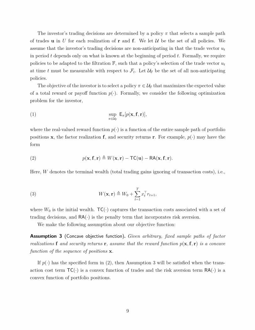
The investor’s trading decisions are determined by a policy π that selects a sample pathof trades u in U for each realization of r and f . We let U be the set of all policies. Weassume that the investor’s trading decisions are non-anticipating in that the trade vector utin period t depends only on what is known at the beginning of period t. Formally, we requirepolicies to be adapted to the filtration F, such that a policy’s selection of the trade vector utat time t must be measurable with respect to Ft. Let UF be the set of all non-anticipatingpolicies.

The objective of the investor is to select a policy π ∈ UF that maximizes the expected valueof a total reward or payoff function p(·). Formally, we consider the following optimizationproblem for the investor,

(1) supπ∈UF

Eπ[p(x, f , r)],

where the real-valued reward function p(·) is a function of the entire sample path of portfoliopositions x, the factor realization f , and security returns r. For example, p(·) may have theform

(2) p(x, f , r) , W (x, r)− TC(u)− RA(x, f , r).

Here, W denotes the terminal wealth (total trading gains ignoring of transaction costs), i.e.,

(3) W (x, r) , W0 +T∑t=1

x>t rt+1,

where W0 is the initial wealth. TC(·) captures the transaction costs associated with a set oftrading decisions, and RA(·) is the penalty term that incorporates risk aversion.

We make the following assumption about our objective function:

Assumption 3 (Concave objective function). Given arbitrary, fixed sample paths of factorrealizations f and security returns r, assume that the reward function p(x, f , r) is a concavefunction of the sequence of positions x.

If p(·) has the specified form in (2), then Assumption 3 will be satisfied when the trans-action cost term TC(·) is a convex function of trades and the risk aversion term RA(·) is aconvex function of portfolio positions.

9

2.1. Examples

In this paper, we consider dynamic portfolio choice models that satisfy Assumptions 1–3.In order to illustrate the generality of this setting, we will now provide a number of specificexamples that satisfy these assumptions.

In many cases, it may be more natural to model the percentage returns associated withan asset, rather than nominal price changes. Our framework accommodates such models, aswe see in the following example:

Example 1 (Models of asset returns). Consider an asset with price Pt, and with log-returnsevolving according to

log(Pt+1

Pt

)= g(Ft, ε(1)

t+1).

Here, Ft is a vector of predictive variables and ε(1)t+1 is an i.i.d. disturbance term. We will

assume that Ft is a Markov process, i.e.,

Ft+1 = h(Ft, ε(2)t+1),

where ε(2)t+1 is another i.i.d. disturbance term.

In this setting, we can define the “factor” process ft , (Pt, Pt−1, Ft). This process evolvesaccording to

ft+1 = Gt+1(ft, εt+1) ,(Pte

g(Ft,ε(1)t+1), Pt, h(Ft, ε(2)

t+1)),

where εt , (ε(1)t , ε

(2)t ). Similarly, define the price change process to be rt , Pt − Pt−1. We

have thatrt+1 = Ht+1(ft, εt+1) , Pte

g(Ft,ε(1)t+1) − Pt,

Then, the joint dynamics of (ft, rt) satisfy Assumption 1.

Note that the Markovian assumption on the predictive variables in Example 1 is just fornotational convenience and is not strictly necessary — we can always augment the vectorwith sufficient history so that the process becomes Markov. What is necessary is only that Ftbe measurable with respect to the filtration generated by the disturbance processes. Indeed,the only real restriction that Assumption 1 imposes is that asset prices are exogenous andare not influenced by trades.

Example 2 (Gârleanu and Pedersen 2013). This model has the following dynamics, wherereturns are driven by mean-reverting factors, that fit into our general framework:

ft+1 = (I − Φ) ft + ε(1)t+1, rt+1 = µt +Bft + ε

(2)t+1,

10

for each time t ≥ 0. Here, µt is the deterministic ‘fair return’, e.g., derived from theCAPM, while B ∈ RN×K is a matrix of constant factor loadings. The factor process ft is avector mean-reverting process, with Φ ∈ RK×K a matrix of mean reversion coefficients forthe factors. It is assumed that the i.i.d. disturbances εt+1 , (ε(1)

t+1, ε(2)t+1) are zero-mean with

covariance given by Var(ε(1)t+1) = Ψ and Var(ε(2)

t+1) = Σ.Trading is costly, and the transaction cost to execute ut = xt − xt−1 shares is given by

TCt(ut) , 12u>t Λut, where Λ ∈ RN×N is a positive semi-definite matrix that measures the level

of trading costs. There are no trading constraints (i.e., U , RN×T ). The investor’s objectivefunction is to choose a trading strategy to maximize discounted future expected excess return,while accounting for transaction costs and adding a per-period penalty for risk, i.e.,

(4) maximizeπ∈UF

Eπ[T∑t=1

(x>t Bft − TCt(ut)− RAt(xt)

)],

where RAt(xt) , γ2x>t Σxt is a per-period risk aversion penalty, with γ being a coefficient

of risk aversion. Gârleanu and Pedersen (2013) suggest this objective function for an in-vestor who is compensated based on his performance relative to a benchmark. Each x>t Bft

term measures the excess return over the benchmark, while each RAt(xt) term measures thevariance of the tracking error relative to the benchmark.4

The problem (4) clearly falls into our framework. The objective function is similar tothat of (2) with the minor variation that expected excess return rather than expected wealthis considered. Further, (4) has the further special property that total transaction costs andpenalty for risk aversion decompose over time:

RA(x, f , r) ,N∑t=1

RAt(xt), TC(u) ,N∑t=1

TCt(ut).

Note that this problem can be handled easily using the classical theory from the linear-quadratic control (LQC) literature (see, e.g., Bertsekas, 2000). This theory provides analyt-ical characterization of optimal solution, for example, that the value function at any time tis quadratic function the state (xt, ft), and that the optimal trade at each time is an affinefunction of the state. Moreover, efficient computational procedures are available to solve forthe optimal policy.

On the other hand, the tractability of this model rests critically on three key requirements:

• The state variables (xt, ft) at each time t must evolve as linear functions of the controlut and the i.i.d. disturbances εt (i.e., linear dynamics).

4See Gârleanu and Pedersen (2013) for other interpretations.

11

• Each control decision ut is unconstrained.

• The objective function must decompose across time into a positive definite quadraticfunction of (xt, ut) at each time t.

These requirements are not satisfied by many real world examples, which may involve port-folio position or trade constraints, different forms of transaction costs and risk measures,and more complicated return dynamics. In the following examples, we will provide concreteexamples of many such cases that do not admit optimal solutions via the LQC methodology,but remain within our framework.

Example 3 (Portfolio or trade constraints). In practice, a common constraint in constructingequity portfolios is the short-sale restriction. Most of the mutual funds are enforced not tohave any short positions by law. This requires the portfolio optimization problem to includethe linear constraint

xt = x0 +t∑

s=1ut ≥ 0,

for each t. This is clearly a convex constraint on the set of feasible trade sequence u.We observe a similar restriction when an execution desk needs to sell or buy a large

portfolio on behalf of an investor. Due to the regulatory rules in agency trading, the executiondesk is only allowed to sell or buy during the trading horizon. In the ‘pure-sell’ scenario, theexecution desk needs to impose the negativity constraint

ut ≤ 0,

for each time t.A third case arises in the context of insurance companies and banks that often need

to satisfy certain minimum capital requirements in order to reduce the risk of insolvency.Therefore, they need to choose a dynamic investment portfolio so that their total wealthnet of transaction costs exceeds a certain threshold C at all times. In our framework, thistranslates into a constraint

W0 +t∑

s=1

(x>s rs+1 − TCs(us)

)≥ C,

for each time t and for each possible realization of returns r. If each transaction cost functionTCs(·) is a convex function, then this constraint is also convex.

Each of the above well-known constraints in portfolio construction fit easily in our frame-work, but cannot be addressed via traditional LQC methods.

12

Example 4 (Non-quadratic transaction costs). In practice, many trading costs such as thebid-ask spread, broker commissions, and exchange fees are intrinsically proportional to thetrade size. Letting χi be the proportional transaction cost rate (an aggregate sum of bid-askcost and commission fees, for example) for trading security i, the investor will incur a totalcost of

TC(u) ,T∑t=1

N∑i=1

χi|ui,t|.

The proportional transaction costs are a classical cost structure that is well studied in theliterature (see, e.g., Constantinides, 1986).

Furthermore, other trading costs occur due to disadvantageous transaction price causedby the price impact of the trade. The management of the trading costs due to price impacthas recently attracted considerable interest (see, e.g., Obizhaeva and Wang, 2005; Almgrenand Chriss, 2000). Many models of transaction costs due to price impact imply a nonlinearrelationship between trade size and the resulting transaction cost, for example

TC(u) ,T∑t=1

N∑i=1

χi|ui,t|β.

Here, β ≥ 1 and χi is a security-specific proportionality constant5.In general, when the trade size is small relative to the total traded volume, proportional

costs will dominate. On the other hand, when the trade size is large, costs due to priceimpact will dominate. Hence, both of these types of trading are important. However, theLQC framework of Example 2 only allows quadratic transaction costs (i.e., β = 2).

Example 5 (Terminal wealth risk). The objective function of Example 2 includes a term topenalize excessive risk. In particular, the per-period quadratic penalty, x>t Σxt, is used, inorder to satisfy the requirements of the LQC model. However, penalizing risk additively ina per-period fashion is nonstandard. Such a risk penalty does not correspond to traditionalforms of investor risk preferences, e.g., maximizing the expected utility of terminal wealth,and the economic meaning of such a penalty is not clear. An investor is typically moreinterested in the risk associated with the terminal wealth, rather than a sum of per-periodpenalties.

In order to account for terminal wealth risk, let ρ : R→ R be a real-valued convex functionmeant to penalize for excessive risk of terminal wealth (e.g., ρ(w) = 1

2w2 for a quadratic

5Gatheral (2010) notes that β = 32 is a typical assumption in practice.

13

penalty) and consider the optimization problem

(5) maximizeπ∈UF

Eπ[W (x, r)− TC(u)− γρ

(W (x, r)

)],

where γ > 0 is a risk-proportionality constant.

It is not difficult to see that the objective in (5) satisfies Assumption 3 and hence fitsinto our model. However, even when the risk penalty function ρ(·) is quadratic, (5) does notadmit a tractable LQC solution, since the quadratic objective does not decompose acrosstime.

Example 6 (Expected utility of terminal wealth). Suppose that U : R → R is an increasingand concave utility function, and consider the optimization problem

(6) maximizeπ∈UF

Eπ[U(W (x, r)− TC(u)

)].

Here, the objective is to maximize the expected utility of terminal wealth net of transactioncosts. If the transaction cost function TC(·) is convex, the objective in (6) is the compositionof a concave and increasing function and a concave function of x; this will be concave andsatisfy Assumption 3.

Note that other mechanisms for risk aversion, such as penalties based on convex orcoherent risk measures, can easily be incorporated in our framework in a manner analogousto Examples 5 and 6.

Example 7 (Maximum drawdown risk). In addition to the terminal measures of risk describedin Example 5, an investor might also be interested in controlling intertemporal measures ofrisk defined over the entire time trajectory. For example, a fund manager might be sensitiveto a string of successive losses that may lead to the withdrawal of assets under management.One way to limit such losses is to control the maximum drawdown, defined as the worst lossof the portfolio between any two points of time during the investment horizon 6. Formally,

MD(x, r) , max1≤t1≤t2≤T

− t2∑t=t1

x>t rt+1, 0 .

It is easy to see that the maximum drawdown is a convex function of x. Hence, the portfoliooptimization problem

(7) maximizeπ∈UF

Eπ[W (x, r)− TC(u)− γMD(x, r)

],

6For example, see Grossman and Zhou (1993) for an earlier example.

14

where γ ≥ 0 is a constant controlling trade-off between wealth and the maximum drawdownpenalty, satisfies Assumption 3. Moreover, standard convex optimization theory yields thatthe problem (7) is equivalent to solving the constrained problem

(8)maximize

π∈UFEπ[W (x, r)− TC(u)

]subject to Eπ [MD(x, r)] ≤ C,

where C (which depends on the choice of γ) is a limit on the allowed expected maximumdrawdown.

Example 8 (Complex dynamics). We can also generalize the dynamics of Example 2. Considerfactor and return dynamics given by

ft+1 = (I − Φ) ft + ε(1)t+1, rt+1 = µt + (B + ξt+1)ft + ε

(2)t+1,

for each time t ≥ 0. Here, each ξt+1 ∈ RN×K is an extra noise term which captures modeluncertainty regarding the factor loadings. We assume that

E [ (B + ξt+1) ft | Ft] = Bft, Var [(B + ξt+1) ft | Ft] = f>t Υf t,

where Ft is the sigma-algebra incorporating all random variables realized by time t, andf t ∈ RK×N is a matrix given by f t ,

[ft ft . . . ft

].

With this model, the conditional variance of returns becomes dependent on the factorstructure and is time-varying, i.e., Var[rt+1|Ft] = f

>t Υf t + Σ. This is consistent with the

empirical work of Fama and French (1996), for example. In this setting, a per-period condi-tional variance risk penalty, analogous to that in (4) becomes RAt(x, f) = x>t

(f>t Υf t + Σ

)xt.

The resulting optimal control problem no longer falls into the LQC framework.

The dynamics and the reward functions considered in these examples satisfy our basicrequirements of Assumptions 1–3. These examples illustrate that in many real-world prob-lems with complex primitives for return predictability, transaction costs, risk measures andconstraints, the dynamic portfolio choice becomes difficult to solve analytically or even usingnumerical methods when the number of assets is large.

3. Optimal Linear ModelThe examples of Section 2.1 illustrated a broad range of important portfolio optimizationproblems. Without special restrictions, such as those imposed in the LQC framework, the

15

optimal dynamic policy for such a broad set of problems cannot be computed either analyt-ically or computationally. In this section, in order to obtain policies in a computationallytractable way, we will consider a more modest goal. Instead of finding the optimal policyamong all admissible dynamic policies, we will restrict our search to a subset of policies thatare parsimoniously parameterized. That is, instead of solving for a globally optimal policy,we will instead find an approximately optimal policy by finding the best policy over therestricted subset of policies.

In order to simplify, we will assume that investor’s reward function in (1) only dependson the sample path of portfolio positions x and of factor realizations f , and does not dependon the security returns r explicitly. In other words, we assume that the reward functiontakes the form p(x, f). This is without loss of generality — given our general specificationfor factors under Assumption 1, we can simply include each security return as a factor. Withthis assumption, investor’s trading decisions will, in general, be a non-anticipating functionof the sample path of factor realizations f . However, consider the following restricted set ofpolicies, linear rebalancing policies, which are obtained by taking the affine combinations ofthe factors:

Definition 1 (Linear rebalancing policy). A linear rebalancing policy π is a non-anticipatingpolicy parameterized by a collection of vectors c , ct ∈ RN , 1 ≤ t ≤ T and a collectionof matrices E , Es,t ∈ RN×K , 1 ≤ s ≤ t ≤ T, that generates a sample path of tradesu , (u1, . . . , uT ) according to

(9) ut , ct +t∑

s=1Es,tfs,

for each time t = 1, 2, . . . , T .Define C to be the set of parameters (E, c) such that the resulting sequence of trades u is

contained in the constraint set U , with probability 1, i.e., u is feasible. Denote by L ⊂ UFthe corresponding set of feasible linear policies.

Observe that linear rebalancing rules allow recourse, albeit in a restricted functional form.The affine specification (9) includes several classes of policies of particular interest as specialcases:

• Deterministic policies. By taking Es,t , 0, for all 1 ≤ s ≤ t ≤ T , it is easy to seethat any deterministic policy is a linear rebalancing policy.

• LQC optimal policies. Optimal portfolios for the LQC framework of Example 2 takethe form xt = Γx,txt−1 + Γf,tft, given matrices Γx,t ∈ RN×N , Γf,t ∈ RN×K , for all

16

1 ≤ t ≤ T , i.e., the optimal portfolio are linear in the previous position and thecurrent factor values. Equivalently, by induction on t,

xt =(

t∏s=1

Γx,s)x0 +

t∑s=1

(s−1∏`=1

Γx,`)

Γf,sfs.

Since ut = xt − xt−1, it is clear that the optimal trade ut is a linear function of thefixed initial position x0, and the factor realizations f1, . . . , ft, and is therefore of theform (9).

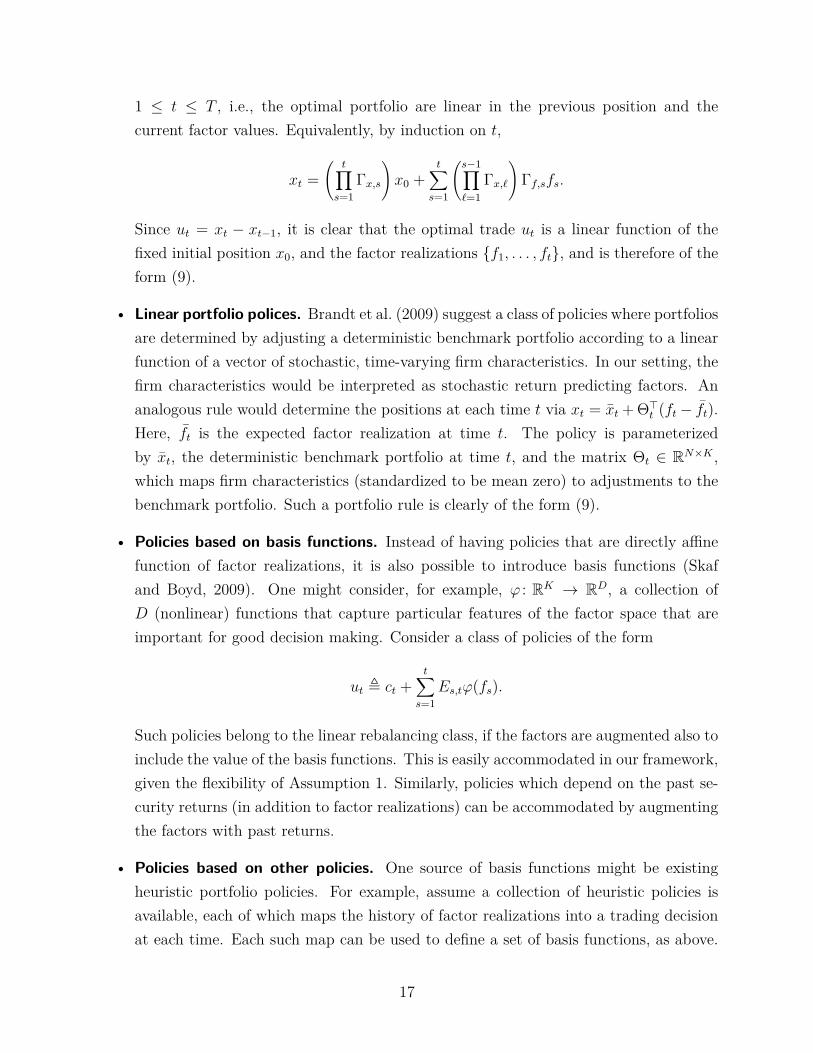
• Linear portfolio polices. Brandt et al. (2009) suggest a class of policies where portfoliosare determined by adjusting a deterministic benchmark portfolio according to a linearfunction of a vector of stochastic, time-varying firm characteristics. In our setting, thefirm characteristics would be interpreted as stochastic return predicting factors. Ananalogous rule would determine the positions at each time t via xt = xt + Θ>t (ft− ft).Here, ft is the expected factor realization at time t. The policy is parameterizedby xt, the deterministic benchmark portfolio at time t, and the matrix Θt ∈ RN×K ,which maps firm characteristics (standardized to be mean zero) to adjustments to thebenchmark portfolio. Such a portfolio rule is clearly of the form (9).

• Policies based on basis functions. Instead of having policies that are directly affinefunction of factor realizations, it is also possible to introduce basis functions (Skafand Boyd, 2009). One might consider, for example, ϕ : RK → RD, a collection ofD (nonlinear) functions that capture particular features of the factor space that areimportant for good decision making. Consider a class of policies of the form

ut , ct +t∑

s=1Es,tϕ(fs).

Such policies belong to the linear rebalancing class, if the factors are augmented also toinclude the value of the basis functions. This is easily accommodated in our framework,given the flexibility of Assumption 1. Similarly, policies which depend on the past se-curity returns (in addition to factor realizations) can be accommodated by augmentingthe factors with past returns.

• Policies based on other policies. One source of basis functions might be existingheuristic portfolio policies. For example, assume a collection of heuristic policies isavailable, each of which maps the history of factor realizations into a trading decisionat each time. Each such map can be used to define a set of basis functions, as above.

17

The corresponding set of linear rebalancing polices would consist of all policies thatare linear combinations of the heuristic policies.

An alternative to solving the original optimal control problem (1) is to consider theproblem

(10) supπ∈L

Eπ[p(x, f)],

restricted to linear rebalancing rules. In general, (10) will not yield an optimal control for(1). The exception is if the optimal control for the problem is indeed a linear rebalancingrule (e.g., in a LQC problem). However, (10) will yield the optimal linear rebalancing rule.Further, in contrast to the original optimal control problem, (10) has the great advantage ofbeing tractable, as suggested by the following result:

Proposition 1. The optimization problem given by

(11)

maximizeE,c

E[p(x, f)

]subject to xt = xt−1 + ut, ∀ 1 ≤ t ≤ T,

ut = ct +t∑

s=1Es,tfs, ∀ 1 ≤ t ≤ T,

(E, c) ∈ C.

is a convex optimization problem, i.e., it involves the maximization of a concave functionsubject to convex constraints.

Proof. Note that p(·, f) is concave for a constant f by Assumption 3. Since x can be writtenas an affine transformation of (E, c), then, for each fixed f , the objective function is concavein (E, c). Taking an expectation over realizations of f preserves this concavity. Finally, theconvexity of the constraint set C follows from the convexity of U , under Assumption 2.

The problem (11) is a finite-dimensional, convex optimization problem that will yieldparameters for the optimal linear rebalancing policy. It is also a stochastic optimizationproblem, in the sense that the objective is the expectation of a random quantity. In general,there are a number of effective numerical methods that can been applied to solve suchproblems:

• Efficient exact formulation. In many cases, with further assumptions on the problemprimitives (the reward function p(·), the dynamics of the factor realizations f , andthe trading constraint set U), the objective E

[p(x, f)

]and the constraint set C of

18

the program (11) can be analytically expressed explicitly in terms of the decisionvariables (E, c). In some of these cases, the program (11) can be transformed into astandard form of convex optimization program such as a quadratic program or a second-order cone program. In such cases, off-the-shelf solvers specialized to these standardforms (e.g., Grant and Boyd, 2011) can be used. Alternatively, generic methods forconstrained convex optimization such as interior point methods (see, e.g., Boyd andVandenberghe, 2004) can be applied to efficiently solve large-scale instances of (11).We will explore this topic further, developing a number of efficient exact formulationsin Appendix A, and providing numerical examples in Sections 4–5.

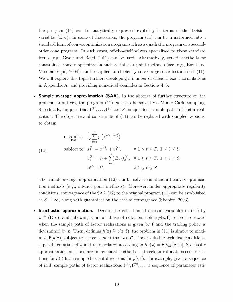
• Sample average approximation (SAA). In the absence of further structure on theproblem primitives, the program (11) can also be solved via Monte Carlo sampling.Specifically, suppose that f (1), . . . , f (S) are S independent sample paths of factor real-ization. The objective and constraints of (11) can be replaced with sampled versions,to obtain

(12)

maximizeE,c

1S

S∑`=1

p(x(`), f (`)

)subject to x

(`)t = x

(`)t−1 + u

(`)t , ∀ 1 ≤ t ≤ T, 1 ≤ ` ≤ S,

u(`)t = ct +

t∑s=1

Es,tf(`)s , ∀ 1 ≤ t ≤ T, 1 ≤ ` ≤ S,

u(`) ∈ U, ∀ 1 ≤ ` ≤ S.

The sample average approximation (12) can be solved via standard convex optimiza-tion methods (e.g., interior point methods). Moreover, under appropriate regularityconditions, convergence of the SAA (12) to the original program (11) can be establishedas S →∞, along with guarantees on the rate of convergence (Shapiro, 2003).

• Stochastic approximation. Denote the collection of decision variables in (11) byz , (E, c), and, allowing a minor abuse of notation, define p(z, f) to be the rewardwhen the sample path of factor realizations is given by f and the trading policy isdetermined by z. Then, defining h(z) , p(z, f), the problem in (11) is simply to maxi-mize E[h(z)] subject to the constraint that z ∈ C. Under suitable technical conditions,super-differentials of h and p are related according to ∂h(z) = E[∂zp(z, f)]. Stochasticapproximation methods are incremental methods that seek to estimate ascent direc-tions for h(·) from sampled ascent directions for p(·, f). For example, given a sequenceof i.i.d. sample paths of factor realizations f (1), f (2), . . ., a sequence of parameter esti-

19

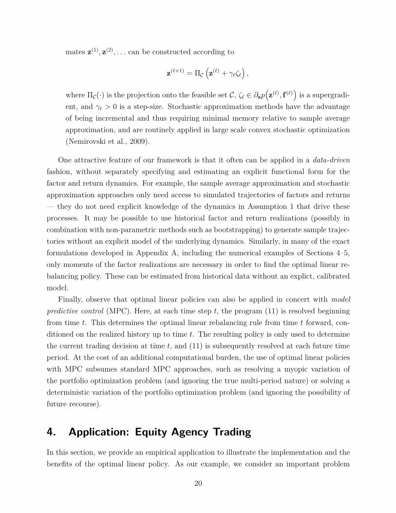
mates z(1), z(2), . . . can be constructed according to

z(`+1) = ΠC(z(`) + γ`ζ`

),

where ΠC(·) is the projection onto the feasible set C, ζ` ∈ ∂zp(z(`), f (`)

)is a supergradi-

ent, and γ` > 0 is a step-size. Stochastic approximation methods have the advantageof being incremental and thus requiring minimal memory relative to sample averageapproximation, and are routinely applied in large scale convex stochastic optimization(Nemirovski et al., 2009).

One attractive feature of our framework is that it often can be applied in a data-drivenfashion, without separately specifying and estimating an explicit functional form for thefactor and return dynamics. For example, the sample average approximation and stochasticapproximation approaches only need access to simulated trajectories of factors and returns— they do not need explicit knowledge of the dynamics in Assumption 1 that drive theseprocesses. It may be possible to use historical factor and return realizations (possibly incombination with non-parametric methods such as bootstrapping) to generate sample trajec-tories without an explicit model of the underlying dynamics. Similarly, in many of the exactformulations developed in Appendix A, including the numerical examples of Sections 4–5,only moments of the factor realizations are necessary in order to find the optimal linear re-balancing policy. These can be estimated from historical data without an explict, calibratedmodel.

Finally, observe that optimal linear policies can also be applied in concert with modelpredictive control (MPC). Here, at each time step t, the program (11) is resolved beginningfrom time t. This determines the optimal linear rebalancing rule from time t forward, con-ditioned on the realized history up to time t. The resulting policy is only used to determinethe current trading decision at time t, and (11) is subsequently resolved at each future timeperiod. At the cost of an additional computational burden, the use of optimal linear policieswith MPC subsumes standard MPC approaches, such as resolving a myopic variation ofthe portfolio optimization problem (and ignoring the true multi-period nature) or solving adeterministic variation of the portfolio optimization problem (and ignoring the possibility offuture recourse).

4. Application: Equity Agency TradingIn this section, we provide an empirical application to illustrate the implementation and thebenefits of the optimal linear policy. As our example, we consider an important problem

20

in equity agency trading. Equity agency trading seeks to address the problem faced bylarge investors such as pension funds, mutual funds, or hedge funds that need to updatethe holdings of large portfolios. Here, the investor seeks to minimize the trading costsassociated with a large portfolio adjustment. These costs, often labeled ‘execution costs’,consist of commissions, bid-ask spreads, and, most importantly in the case of large trades,price impact from trading. Efficient execution of large trades is accomplished via ‘algorithmictrading’, and requires significant technical expertise and infrastructure. For this reason, largeinvestors utilize algorithmic trading service providers, such as execution desks in investmentbanks. Such services are often provided on an agency basis, where the execution desk tradeson behalf of the client, in exchange for a fee. The responsibility of the execution desk is tofind a feasible execution schedule over the client-specified trading horizon while minimizingtrading costs and aligning with the risk objectives of the client.

The problem of finding an optimal execution schedule has received a lot of attention inthe literature since the initial paper of Bertsimas and Lo (1998). In their model, when priceimpact is proportional to the number of shares traded, the optimal execution schedule is totrade equal number of shares at each trading time. There are number of papers that extendthis model to incorporate the risk of the execution strategy. For example, Almgren andChriss (2000) derive that risk averse agents need to liquidate their portfolio faster in orderto reduce the uncertainty of the execution cost.

The models described above seek mainly to minimize execution costs by accounting forthe price impact and supply/demand imbalances caused by the investor’s trading. Comple-mentary to this, an investor may also seek to exploit short-term predictability of stock returnsto inform the design of a trade schedule. As such, there is a growing interest to model returnpredictability in intraday stock returns. Often called ‘short-term alpha models’, some of thepredictive models are similar to well-known factor models for the study of long-term stockreturns, e.g., the Capital Asset Pricing Model (CAPM), or the Fama-French Three FactorModel. Alternatively, short-term predictions can be developed from microstructure effects,for example the imbalance of orders in an electronic limit order book. Heston et al. (2010)document that systematic trading as described in the examples above and institutional fundflows lead to predictable patterns in intraday returns of common stocks.

We will consider an agency trading optimal execution problem in the presence of short-term predictability. One issue that arises here is that, due to the regulatory rules in agencytrading, the execution desk is only allowed to either sell or buy a particular security overthe course of the trading horizon, depending on whether the ultimate position adjustmentdesired for that security is negative or positive. However, given a model for short-termpredictability, an optimal trading policy that minimizes execution cost may result in both

21

buy and sell trades for the same security as it seeks to exploit short-term signals. Hence, itis necessary to impose constraints on the sign of trades, as in Example 3.

If an agency trading execution problem has price and factor dynamics which satisfyAssumption 1 and an objective (including transaction costs, price impact, and risk aversion)that satisfies Assumption 3, then we can compute the best execution schedule in the spaceof linear execution schedules, i.e., the number of shares to trade at each time is a linearfunction of the previous return predicting factors. We will consider a particular formulationthat involves linear price and factor dynamics and a quadratic objective function (as inExample 2). Note that this example does not highlight the full generality of our framework— more interesting cases would involve nonlinear factor dynamics (e.g., microstructure-based order imbalance signals) or a non-quadratic objective (e.g., transaction costs as inExample 4). However, this example is intentionally chosen since, in the absence of the tradesign constraint, the problem can be solved exactly with LQC methods. Hence, we are ableto compare the optimal linear policy to policies derived from LQC methods applied to theunconstrained problem.

The rest of this section is organized as follows. We present our optimal execution problemformulation in Section 4.1. An exact, analytical solution is not available to this problem,hence, in Section 4.2, we describe several approximate solution techniques, including findingthe best linear policy. In order to evaluate the quality of the approximate methods, inSection 4.3, we describe several techniques for computing upper bounds on the performance ofany policy for our execution problem. In Section 4.4, we describe the empirical calibration ofthe parameters of our problem. Finally, in Section 4.5, we present and discuss the numericalresults.

4.1. Formulation

We follow the general framework of Section 2. Suppose that x0 ∈ RN denotes the numberof shares in each of N securities that we would like to sell before time T . We assume thattrades can occur at discrete times, t = 1, . . . , T . We define an execution schedule to be thecollection u , (u1, . . . , uT ), where each ut ∈ RN denotes the number of shares traded at timet. Note that a negative (positive) value of ui,t denotes a sell (buy) trade of security i at timet. The total position at time t is given by xt = x0 +∑t

s=1 us.The formulation of the agency trading optimal execution problem is as follows:

• Constraints. Without loss of generality, we will assume that the initial position ispositive, i.e., x0 > 0. The execution schedule must liquidate the entire initial position

22

by the end of the time horizon, thus

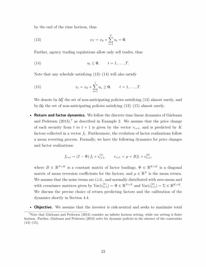
(13) xT = x0 +T∑t=1

ut = 0.

Further, agency trading regulations allow only sell trades, thus

(14) ut ≤ 0, t = 1, . . . , T.

Note that any schedule satisfying (13)–(14) will also satisfy

(15) xt = x0 +t∑

s=1us ≥ 0, t = 1, . . . , T.

We denote by U0F the set of non-anticipating policies satisfying (13) almost surely, and

by UF the set of non-anticipating policies satisfying (13)–(15) almost surely.

• Return and factor dynamics. We follow the discrete time linear dynamics of Gârleanuand Pedersen (2013),7 as described in Example 2. We assume that the price changeof each security from t to t + 1 is given by the vector rt+1, and is predicted by K

factors collected in a vector ft. Furthermore, the evolution of factor realizations followa mean reverting process. Formally, we have the following dynamics for price changesand factor realizations:

ft+1 = (I − Φ) ft + ε(1)t+1, rt+1 = µ+Bft + ε

(2)t+1,

where B ∈ RN×K is a constant matrix of factor loadings, Φ ∈ RK×K is a diagonalmatrix of mean reversion coefficients for the factors, and µ ∈ RN is the mean return.We assume that the noise terms are i.i.d., and normally distributed with zero-mean andwith covariance matrices given by Var(ε(1)

t+1) = Ψ ∈ RN×N and Var(ε(2)t+1) = Σ ∈ RK×K .

We discuss the precise choice of return predicting factors and the calibration of thedynamics shortly in Section 4.4.

• Objective. We assume that the investor is risk-neutral and seeks to maximize total7Note that Gârleanu and Pedersen (2013) consider an infinite horizon setting, while our setting is finite

horizon. Further, Gârleanu and Pedersen (2013) solve for dynamic policies in the absence of the constraints(13)–(15).

23

excess profits after quadratic transaction costs, i.e.,

(16) V∗ , maximizeπ∈UF

Eπ[T∑t=1

(x>t Bft − 1

2u>t Λut

)],

where Λ ∈ RN×N is a matrix parameterizing the quadratic transaction costs.

Note that the problem (16) is a special case of the optimization program in Example 2, withthe exception of the constraints (13)–(15).

4.2. Approximate Policies

Since a tractable analytical or computational solution to the optimal execution problem in(16) is not available, we compare four approximate solution techniques:

• TWAP. A time-weighted average price (TWAP) policy seeks to sell a fixed quantityut = −x0/T of shares in each of the T periods. This policy minimizes transactioncosts, and would be optimal in the absence of a predictive model for returns.

• Deterministic. Instead of allowing for a non-anticipating dynamic policy, where thetrade at each time t is allowed to depend on all events that have occurred before t, wecan solve for an optimal static policy, i.e., a deterministic sequence of trades over theentire time horizon that is decided at the beginning of the time horizon. Here, observethat at the beginning of the time horizon, the expected future factor vector is given byE[ft|f0] = (I−Φ)tf0. Therefore, in order to find the optimal deterministic policy, givenf0, we maximize the conditional expected value of the stochastic objective in (16) bysolving the quadratic program

(17)

maximizeu

T∑t=1

(x>t B(I − Φ)tf0 − 1

2u>t Λut

)subject to ut = xt − xt−1, t = 1, . . . , T,

ut ≤ 0, xt ≥ 0, t = 1, . . . , T,xT = 0,

to yield a deterministic sequence of trades u.

• Model predictive control. In this approximation, at each trading time, we solvefor the deterministic sequence of trades conditional on the available information andimplement only the first trade. Thus, this policy is an immediate extension of the

24

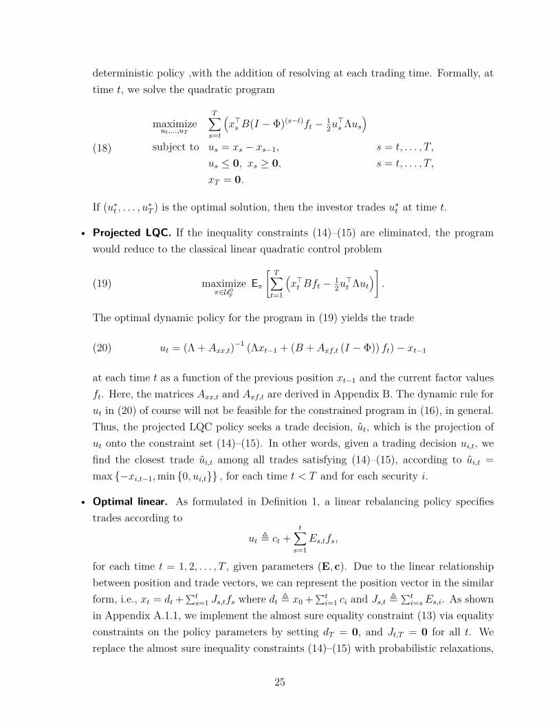
deterministic policy ,with the addition of resolving at each trading time. Formally, attime t, we solve the quadratic program

(18)

maximizeut,...,uT

T∑s=t

(x>s B(I − Φ)(s−t)ft − 1

2u>s Λus

)subject to us = xs − xs−1, s = t, . . . , T,

us ≤ 0, xs ≥ 0, s = t, . . . , T,

xT = 0.

If (u∗t , . . . , u∗T ) is the optimal solution, then the investor trades u∗t at time t.

• Projected LQC. If the inequality constraints (14)–(15) are eliminated, the programwould reduce to the classical linear quadratic control problem

(19) maximizeπ∈U0

F

Eπ[T∑t=1

(x>t Bft − 1

2u>t Λut

)].

The optimal dynamic policy for the program in (19) yields the trade

(20) ut = (Λ + Axx,t)−1 (Λxt−1 + (B + Axf,t (I − Φ)) ft)− xt−1

at each time t as a function of the previous position xt−1 and the current factor valuesft. Here, the matrices Axx,t and Axf,t are derived in Appendix B. The dynamic rule forut in (20) of course will not be feasible for the constrained program in (16), in general.Thus, the projected LQC policy seeks a trade decision, ut, which is the projection ofut onto the constraint set (14)–(15). In other words, given a trading decision ui,t, wefind the closest trade ui,t among all trades satisfying (14)–(15), according to ui,t =max −xi,t−1,min 0, ui,t , for each time t < T and for each security i.

• Optimal linear. As formulated in Definition 1, a linear rebalancing policy specifiestrades according to

ut , ct +t∑

s=1Es,tfs,

for each time t = 1, 2, . . . , T , given parameters (E, c). Due to the linear relationshipbetween position and trade vectors, we can represent the position vector in the similarform, i.e., xt = dt +∑t

s=1 Js,tfs where dt , x0 +∑ti=1 ci and Js,t ,

∑ti=sEs,i. As shown

in Appendix A.1.1, we implement the almost sure equality constraint (13) via equalityconstraints on the policy parameters by setting dT = 0, and Jt,T = 0 for all t. Wereplace the almost sure inequality constraints (14)–(15) with probabilistic relaxations,

25

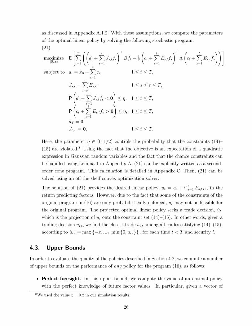
as discussed in Appendix A.1.2. With these assumptions, we compute the parametersof the optimal linear policy by solving the following stochastic program:(21)

maximize(E,c)

E T∑t=1

(dt +t∑

s=1Js,tfs

)>Bft − 1

2

(ct +

t∑s=1

Es,tfs

)>Λ(ct +

t∑s=1

Es,tfs

)subject to dt = x0 +

t∑i=1

ci, 1 ≤ t ≤ T,

Js,t =t∑i=s

Es,i, 1 ≤ s ≤ t ≤ T,

P(dt +

t∑s=1

Js,tfs < 0)≤ η, 1 ≤ t ≤ T,

P(ct +

t∑s=1

Es,tfs > 0)≤ η, 1 ≤ t ≤ T,

dT = 0,Jt,T = 0, 1 ≤ t ≤ T.

Here, the parameter η ∈ (0, 1/2) controls the probability that the constraints (14)–(15) are violated.8 Using the fact that the objective is an expectation of a quadraticexpression in Gaussian random variables and the fact that the chance constraints canbe handled using Lemma 1 in Appendix A, (21) can be explicitly written as a second-order cone program. This calculation is detailed in Appendix C. Then, (21) can besolved using an off-the-shelf convex optimization solver.

The solution of (21) provides the desired linear policy, ut = ct + ∑ts=1 Es,tfs, in the

return predicting factors. However, due to the fact that some of the constraints of theoriginal program in (16) are only probabilistically enforced, ut may not be feasible forthe original program. The projected optimal linear policy seeks a trade decision, ut,which is the projection of ut onto the constraint set (14)–(15). In other words, given atrading decision ui,t, we find the closest trade ui,t among all trades satisfying (14)–(15),according to ui,t = max −xi,t−1,min 0, ui,t , for each time t < T and security i.

4.3. Upper Bounds

In order to evaluate the quality of the policies described in Section 4.2, we compute a numberof upper bounds on the performance of any policy for the program (16), as follows:

• Perfect foresight. In this upper bound, we compute the value of an optimal policywith the perfect knowledge of future factor values. In particular, given a vector of

8We used the value η = 0.2 in our simulation results.

26

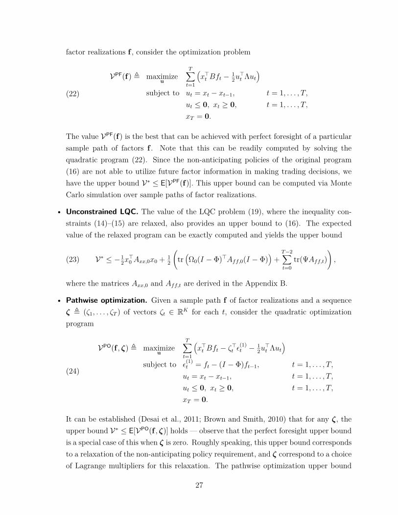
factor realizations f , consider the optimization problem

(22)

VPF(f) , maximizeu

T∑t=1

(x>t Bft − 1

2u>t Λut

)subject to ut = xt − xt−1, t = 1, . . . , T,

ut ≤ 0, xt ≥ 0, t = 1, . . . , T,xT = 0.

The value VPF(f) is the best that can be achieved with perfect foresight of a particularsample path of factors f . Note that this can be readily computed by solving thequadratic program (22). Since the non-anticipating policies of the original program(16) are not able to utilize future factor information in making trading decisions, wehave the upper bound V∗ ≤ E[VPF(f)]. This upper bound can be computed via MonteCarlo simulation over sample paths of factor realizations.

• Unconstrained LQC. The value of the LQC problem (19), where the inequality con-straints (14)–(15) are relaxed, also provides an upper bound to (16). The expectedvalue of the relaxed program can be exactly computed and yields the upper bound

(23) V∗ ≤ −12x>0 Axx,0x0 + 1

2

(tr(Ω0(I − Φ)>Aff,0(I − Φ)

)+

T−2∑t=0

tr(ΨAff,t)),

where the matrices Axx,0 and Aff,t are derived in the Appendix B.

• Pathwise optimization. Given a sample path f of factor realizations and a sequenceζ , (ζ1, . . . , ζT ) of vectors ζt ∈ RK for each t, consider the quadratic optimizationprogram

(24)

VPO(f , ζ) , maximizeu

T∑t=1

(x>t Bft − ζ>t ε

(1)t − 1

2u>t Λut

)subject to ε

(1)t = ft − (I − Φ)ft−1, t = 1, . . . , T,ut = xt − xt−1, t = 1, . . . , T,ut ≤ 0, xt ≥ 0, t = 1, . . . , T,xT = 0.

It can be established (Desai et al., 2011; Brown and Smith, 2010) that for any ζ, theupper bound V∗ ≤ E[VPO(f , ζ)] holds — observe that the perfect foresight upper boundis a special case of this when ζ is zero. Roughly speaking, this upper bound correspondsto a relaxation of the non-anticipating policy requirement, and ζ correspond to a choiceof Lagrange multipliers for this relaxation. The pathwise optimization upper bound

27

corresponds to making a choice for ζ that results in an optimal upper bound, i.e.,V∗ ≤ minζ E[VPO(f , ζ)]. This minimization involves a convex objective function andcan be computed via stochastic gradient descent; we refer the reader to Desai et al.(2011) for details.

4.4. Model Calibration

In this section, we describe calibration of the parameters of the optimal execution problemformulated in Section 4.1. We chose one of the most liquid stocks, Apple, Inc. (NASDAQ:AAPL), for our empirical study. We set the execution horizon to be 1 hour and trade intervalsto be 5 minutes. Thus, setting a trade interval to be a one unit of time, we have a timehorizon of T = 12, We assume that the initial position to be liquidated is x0 = 100,000shares.

In trade execution problems, the time horizon is typically a day, thus we will constructa factor model in the same time-frequency. We will use the intraday transaction prices ofAAPL from the NYSE TAQ database on the trading days of January 4, 2010 (day 0) andJanuary 5, 2010 (day 1) to construct K = 2 return predicting factors, each with a differentmean reversion speed. We first divide each trading day into 78 time intervals, each 5 minutesin length. For each 5 minute interval, we calculate the average transaction price from alltransactions in that interval. Let p(d)

t be the average price for interval t = 1, . . . , 78 on dayd = 0, 1. Let fk,t be the value of factor k = 1, 2 for interval t = 2, . . . , 78, defined as follows

f1,t , p(1)t − p

(1)t−1, f2,t , p

(1)t − p

(0)t .

In other words, f1,t is the average price change over the previous 5 minute interval, while f2,t

is the average price change relative to the previous day. Here, we can interpret the factorsas the representations of value and momentum signals. Intuitively, the first factor can beconsidered as a ‘momentum’-type signal with fast mean reversion and the second factor asa ‘value’-type signal with slow mean reversion.

Given the price change of the security rt+1 , p(1)t+1 − p

(1)t , we can compute the estimate

of the factor loading matrix, B, using the following linear regression:

rt+1 = 0.0726 + 0.3375 f1,t − 0.0720 f2,t + ε(2)t+1,

(1.96) (3.11) (−2.2)

where the OLS t-statistics are reported in brackets. Thus,

B =[0.3375 −0.072

].

28

Similarly, we obtain the mean reversion rates for the factors,

∆f1,t+1 = −0.7146 f1,t + ε(1)1,t+1, ∆f2,t+1 = −0.0353 f2,t + ε

(1)2,t+1.

(−6.62) (−1.16)

Thus,

Φ =0.7146 0

0 0.0353

.The variance of the error terms is estimated to be

Σ , Var(ε(2)t ) = 0.0428, Ψ , Var(ε(1)

t ) =0.0378 0

0 0.0947

.The distribution of the initial factor realization, f0, is set to the stationary distribu-

tion under the given factor dynamics, i.e., f0 is normally distributed with zero mean andcovariance

Ω0 ,∞∑t=1

(I − Φ)t Ψ (I − Φ)t =0.0412 0

0 1.3655

.A rough estimate of the transaction cost coefficient Λ = 2.14×10−5 is used — this implies

a transaction cost of $10 or 0.5 basis points on a typical trade of 1,000 shares.

4.5. Numerical Results

Using the calibrated parameters from Section 4.4, we run a simulation with 50,000 trials toestimate the performance of each of the approximate policies of Section 4.2. In each trial,we sample the initial factor f0, solve for the resulting policy of each approximate method,and compute its corresponding payoff. In order to evaluate the performance of each policyeffectively, we use the same set of simulation paths in each policy’s computation of averagepayoff. We used CVX (Grant and Boyd, 2011), a package for solving convex optimizationproblems in Matlab, to solve the optimization problems that occur in the computation ofthe deterministic, model predictive control, and optimal linear policies.

The upper half of Table 1 summarizes the performance of each of the policies describedin Section 4.2. For each policy, we divide the total payoff into two components, the alphagains (i.e., ∑T

t=1 x>t Bft) and the transaction costs (i.e., ∑T

t=1−u>t Λut). For each of thesecomponents as well as the total, we report the mean value over all simulation trials and theassociated standard error.9 In the lower half of Table 1, we report upper bounds on the

9Note that values for the TWAP policy and the unconstrained LQC upper bound are computed exactlywithout Monte Carlo simulation.

29

Alpha T.C. Total Optimality CPU time($k) ($k) ($k) Gap (sec)

Policies

TWAP Mean 0.03 -8.91 -8.88 238% <0.01S.E. 0.210 0.000 0.210

Deterministic Mean 19.34 -15.81 3.53 45.4% 0.82S.E. 0.229 0.025 0.224

Model predictive control Mean 21.25 -16.54 4.71 27.1% 5.79S.E. 0.233 0.023 0.225

Projected LQC Mean 25.13 -19.40 5.73 11.3% 0.02S.E. 0.227 0.039 0.229

Optimal linear Mean 23.24 -17.11 6.13 5.11% 4.23S.E. 0.233 0.025 0.224

UpperBounds

Pathwise optimization Mean 6.46

S.E. 0.04

Perfect foresight Mean 8.57S.E. 0.223

Unconstrained LQC Mean 12.58

Table 1: Summary of the performance statistics of each policy in the optimal executionexample, along with upper bounds. In the upper half of the table we consider the approximatepolicies. For each approximate policy, we divide the total payoff into two components, thealpha gains and the transaction costs. For each performance statistic, we report the meanvalue and the associated standard error. Finally, we report the average computation time (inseconds) for each policy per simulation trial. In the bottom half of the table, we report thecomputed upper bounds on the total payoff. For those methods which involve Monte Carlosimulation, standard errors are also reported.

total payoff of any policy, as computed using the methods described in Section 4.3. Thepathwise optimization method achieves the tightest upper bound. For each policy, we reportan optimality gap relative to this tightest upper bound.

Comparing the performance of the various policies in Table 1, we see accounting forpredictable price movements can make a significant difference. Indeed, the TWAP policy,which minimizes transaction costs but ignores predictable price movements, performs theworst. Other policies incur higher transaction costs than TWAP but more than make upfor this by opportunistically timing the liquidation relative to predictable price movements.Of the remaining policies, the projected LQC and optimal linear policies achieve the highestperformance. These are the only policies that are constructed in a manner that explicitlyaccount for the dynamic multi-period nature of the problem and allow for recourse.

The overall best policy is the optimal linear policy, which achieves a value that is within5% of the value that can be achieved by any policy. This optimality gap is a factor of

30

(Optimal Linear)− (Projected LQC)Alpha T.C. Total($k) ($k) ($k)

Mean -1.89 2.29 0.40S.E. 0.0137 0.0196 0.0095

Table 2: A detailed comparison of the difference in alpha gains, transaction costs, and totalperformance between the optimal linear policy and projected dynamic policy in the optimalexecution example. We observe that the standard error for the difference in total payoff isvery small, thus, the performance gain by employing the optimal linear policy is statisticallysignificant.

two improvement over the optimality gap of the next best policy, projected LQC, and issignificantly better than any other policy.

Note that, despite the higher total payoff for the optimal linear policy as compared to theprojected LQC policy in Table 1, the relatively high standard errors preclude the immediateconclusion that the optimal linear policy achieves a statistically significant higher total payoff.Thus, in order to provide a more careful comparison, for each simulation trial, we considerthe difference in alpha gains, transaction costs, and total payoff between these two policies.Table 2 show the statistics of these differences, and establishes that the performance benefitof the optimal linear policy is statistically significant. Moreover, Table 2 reveals that theoptimal linear policy achieves a better result by more carefully managing transaction costs,at the expense of not achieving the alpha gains of the projected LQC policy.

In Table 1, we also report the average computation time (in seconds) required to evaluateeach policy for over a single simulated sample path. This gives a sense of the relativecomputational complexity of the various policies. The TWAP and projected LQC policiesare the fastest to evaluate — the former is essentially trivial, while the latter has a closed-formexpression (via a solution of recursive equations). The remaining policies involve solving atleast one optimization problem per sample path. These policies have roughly the same orderof magnitude in computation time, with model predictive control (which solves a differentoptimization problem at every time step) having the longest running time.

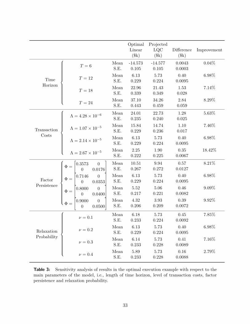
4.6. Sensitivity Results

In Table 3, we report the sensitivity of our simulation results with respect to main parametersof the optimal execution problem, e.g., length of time horizon, level of transaction costs, levelof factor persistence and relaxation probability. We only vary the parameter at hand whilekeeping the other parameters fixed. We report the average objective value and its standard

31

error for the optimal linear and projected LQC policies, the top performing policies in ourbaseline simulation.

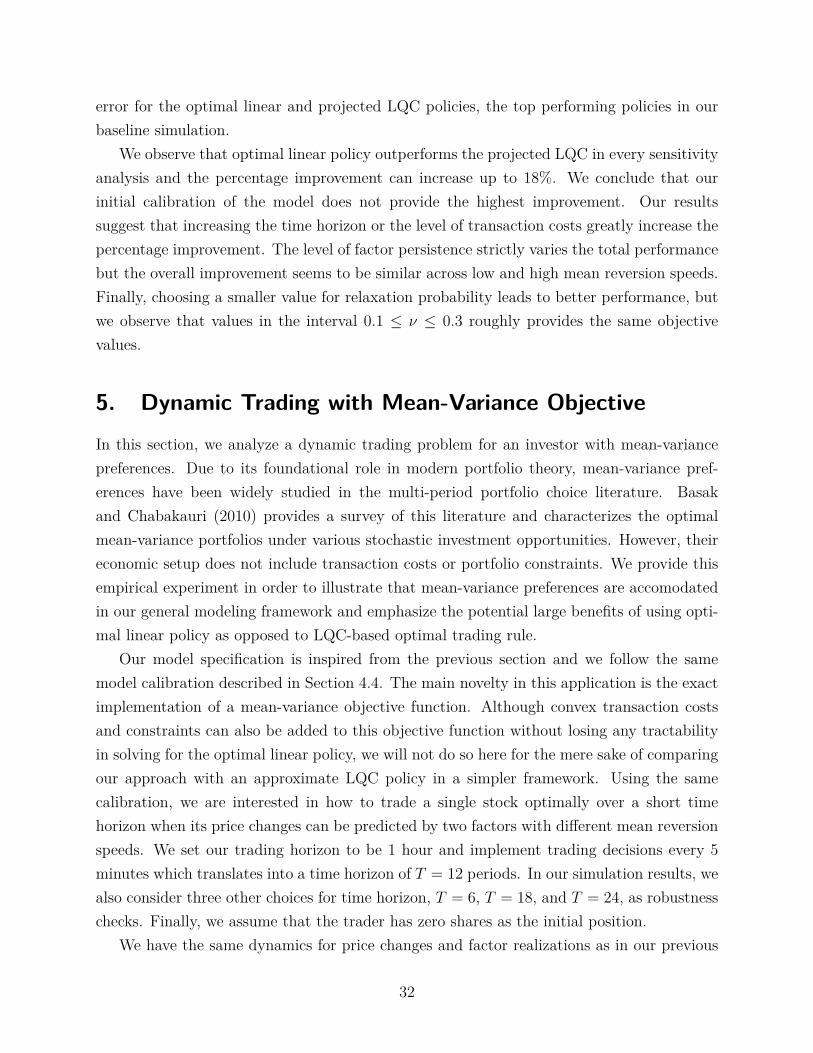
We observe that optimal linear policy outperforms the projected LQC in every sensitivityanalysis and the percentage improvement can increase up to 18%. We conclude that ourinitial calibration of the model does not provide the highest improvement. Our resultssuggest that increasing the time horizon or the level of transaction costs greatly increase thepercentage improvement. The level of factor persistence strictly varies the total performancebut the overall improvement seems to be similar across low and high mean reversion speeds.Finally, choosing a smaller value for relaxation probability leads to better performance, butwe observe that values in the interval 0.1 ≤ ν ≤ 0.3 roughly provides the same objectivevalues.

5. Dynamic Trading with Mean-Variance ObjectiveIn this section, we analyze a dynamic trading problem for an investor with mean-variancepreferences. Due to its foundational role in modern portfolio theory, mean-variance pref-erences have been widely studied in the multi-period portfolio choice literature. Basakand Chabakauri (2010) provides a survey of this literature and characterizes the optimalmean-variance portfolios under various stochastic investment opportunities. However, theireconomic setup does not include transaction costs or portfolio constraints. We provide thisempirical experiment in order to illustrate that mean-variance preferences are accomodatedin our general modeling framework and emphasize the potential large benefits of using opti-mal linear policy as opposed to LQC-based optimal trading rule.

Our model specification is inspired from the previous section and we follow the samemodel calibration described in Section 4.4. The main novelty in this application is the exactimplementation of a mean-variance objective function. Although convex transaction costsand constraints can also be added to this objective function without losing any tractabilityin solving for the optimal linear policy, we will not do so here for the mere sake of comparingour approach with an approximate LQC policy in a simpler framework. Using the samecalibration, we are interested in how to trade a single stock optimally over a short timehorizon when its price changes can be predicted by two factors with different mean reversionspeeds. We set our trading horizon to be 1 hour and implement trading decisions every 5minutes which translates into a time horizon of T = 12 periods. In our simulation results, wealso consider three other choices for time horizon, T = 6, T = 18, and T = 24, as robustnesschecks. Finally, we assume that the trader has zero shares as the initial position.

We have the same dynamics for price changes and factor realizations as in our previous

32

Optimal ProjectedLinear LQC Difference Improvement($k) ($k) ($k)

TimeHorizon

T = 6 Mean -14.573 -14.577 0.0043 0.04%S.E. 0.105 0.105 0.0003

T = 12 Mean 6.13 5.73 0.40 6.98%S.E. 0.229 0.224 0.0095

T = 18 Mean 22.96 21.43 1.53 7.14%S.E. 0.339 0.349 0.028

T = 24 Mean 37.10 34.26 2.84 8.29%S.E. 0.443 0.459 0.059

TransactionCosts

Λ = 4.28× 10−6 Mean 24.01 22.73 1.28 5.63%S.E. 0.235 0.240 0.025

Λ = 1.07× 10−5 Mean 15.84 14.74 1.10 7.46%S.E. 0.229 0.236 0.017

Λ = 2.14× 10−5 Mean 6.13 5.73 0.40 6.98%S.E. 0.229 0.224 0.0095

Λ = 2.67× 10−5 Mean 2.25 1.90 0.35 18.42%S.E. 0.222 0.225 0.0067

FactorPersistence

Φ =[0.3573 0

0 0.0176

]Mean 10.51 9.94 0.57 8.21%S.E. 0.267 0.272 0.0127

Φ =[0.7146 0

0 0.0353

]Mean 6.13 5.73 0.40 6.98%S.E. 0.229 0.224 0.0095

Φ =[0.8000 0

0 0.0400

]Mean 5.52 5.06 0.46 9.09%S.E. 0.217 0.221 0.0082

Φ =[0.9000 0

0 0.0500

]Mean 4.32 3.93 0.39 9.92%S.E. 0.206 0.209 0.0072

RelaxationProbability

ν = 0.1 Mean 6.18 5.73 0.45 7.85%S.E. 0.233 0.224 0.0092

ν = 0.2 Mean 6.13 5.73 0.40 6.98%S.E. 0.229 0.224 0.0095

ν = 0.3 Mean 6.14 5.73 0.41 7.16%S.E. 0.233 0.228 0.0089

ν = 0.4 Mean 5.89 5.73 0.16 2.79%S.E. 0.233 0.228 0.0088

Table 3: Sensitivity analysis of results in the optimal execution example with respect to themain parameters of the model, i.e., length of time horizon, level of transaction costs, factorpersistence and relaxation probability.

33

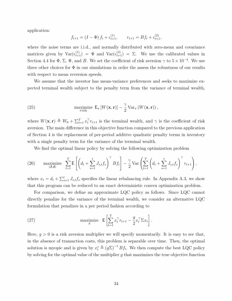
application:ft+1 = (I − Φ) ft + ε

(1)t+1, rt+1 = Bft + ε

(2)t+1,

where the noise terms are i.i.d., and normally distributed with zero-mean and covariancematrices given by Var(ε(1)

t+1) = Ψ and Var(ε(2)t+1) = Σ. We use the calibrated values in

Section 4.4 for Φ, Σ, Ψ, and B. We set the coefficient of risk aversion γ to 5× 10−4. We usethree other choices for Φ in our simulations in order the assess the robustness of our resultswith respect to mean reversion speeds.

We assume that the investor has mean-variance preferences and seeks to maximize ex-pected terminal wealth subject to the penalty term from the variance of terminal wealth,

(25) maximizeπ∈UF

Eπ [W (x, r)]− γ

2 Varπ (W (x, r)) ,

where W (x, r) , W0 + ∑Tt=1 x

>t rt+1 is the terminal wealth, and γ is the coefficient of risk

aversion. The main difference in this objective function compared to the previous applicationof Section 4 is the replacement of per-period additive quadratic penalty terms in inventorywith a single penalty term for the variance of the terminal wealth.

We find the optimal linear policy by solving the following optimization problem

(26) maximize(J,d)

T∑t=1

E(dt +

t∑s=1

Js,tfs

)>Bft

− γ

2 Var T∑t=1

(dt +

t∑s=1

Js,tfs

)>rt+1

,where xt = dt +∑t

s=1 Js,tfs specifies the linear rebalancing rule. In Appendix A.3, we showthat this program can be reduced to an exact deterministic convex optimization problem.

For comparison, we define an approximate LQC policy as follows. Since LQC cannotdirectly penalize for the variance of the terminal wealth, we consider an alternative LQCformulation that penalizes in a per period fashion according to

(27) maximizeg

E[T∑t=1

x>t rt+1 −g

2x>t Σxt

].

Here, g > 0 is a risk aversion multiplier we will specify momentarily. It is easy to see that,in the absence of transaction costs, this problem is separable over time. Then, the optimalsolution is myopic and is given by x∗t , (gΣ)−1 Bft. We then compute the best LQC policyby solving for the optimal value of the multiplier g that maximizes the true objective function

34

with the variance penalty,

(28)maximize

gE[T∑t=1

x>t rt+1

]− γ

2 Var(

T∑t=1

x>t rt+1

)subject to xt = (gΣ)−1 Bft, 1 ≤ t ≤ T.

Then, letting xt = (g∗Σ)−1 Bft provides an approximate LQC policy.In Table 4 and Table 5, we report the simulation results from 50, 000 trials illustrating

the performance differential of optimal linear policy and LQC policy under four differentchoices of time horizon and mean reversion speeds for the return predicting factors10.

We observe that optimal linear policy outperforms the LQC policy substantially in everycase and the percentage improvement in the objective value can increase up to 72%. Ourresults suggest that increasing the time horizon and the level of persistence in the signals ispositively related with the corresponding percentage improvement.

6. ConclusionThis paper provides a highly tractable formulation for determining rebalancing rules indynamic portfolio choice problems involving complex models of return predictability. Ourrebalancing rule is a linear function of past return predicting factors and can be utilized ina wide spectrum of portfolio choice models with realistic considerations for risk measures,transaction costs, and trading constraints. We illustrate the broad utility of our method byshowing its applicability across a broad range of modeling assumptions on these portfoliooptimization primitives. As long as the underlying dynamic portfolio optimization problemis a convex programming problem (i.e., concave objective and convex decision constraints),the modified optimization problem seeking the optimal parameters of the linear decisionrule will be a convex programming problem that is tractable numerically. We demonstratein realistic numerical experiments that such modeling flexibility can offer significant practicalbenefits.

ReferencesR. F. Almgren and N. Chriss. Optimal execution of portfolio transactions. Journal of Risk, 3(2):

5–39, 2000.

P. Balduzzi and A. W. Lynch. Transaction costs and predictability: some utility cost calculations.Journal of Financial Economics, 52(1):47–78, apr 1999.10Our simulation results across different values of Σ and γ simply scale the objective value by the ratio of

these parameter values. Hence, we omit a sensitivity analysis on these parameters.

35

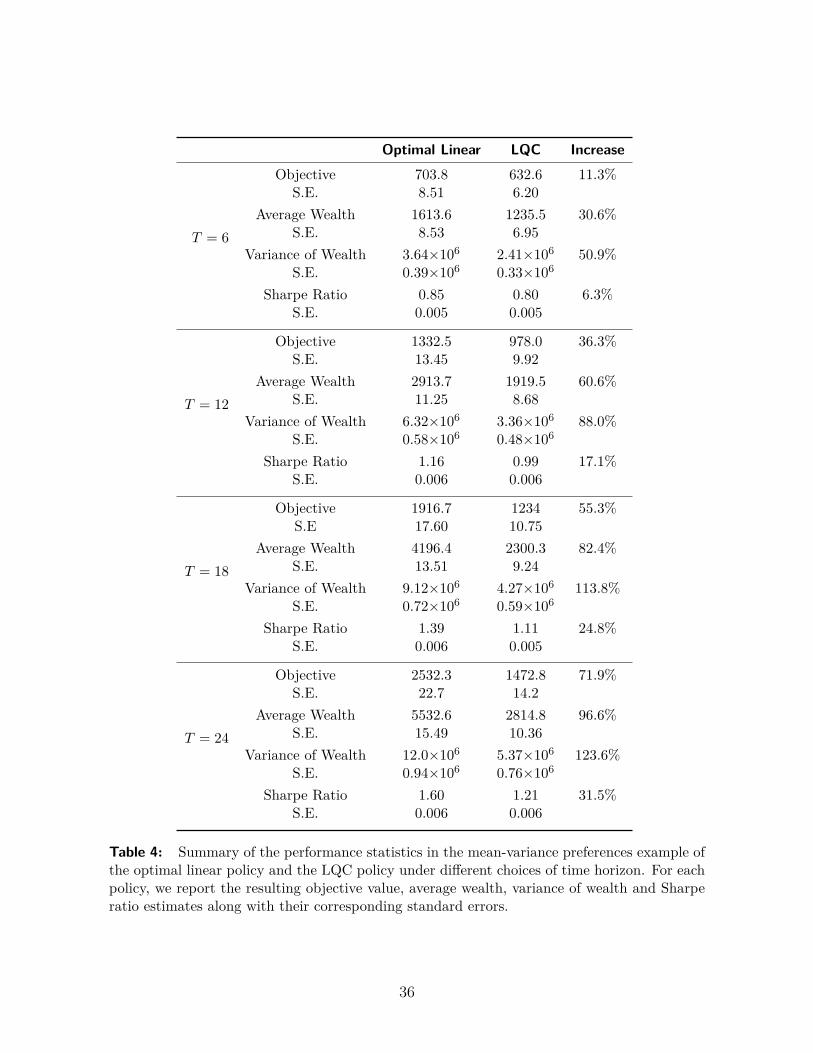
Optimal Linear LQC Increase

T = 6

Objective 703.8 632.6 11.3%S.E. 8.51 6.20

Average Wealth 1613.6 1235.5 30.6%S.E. 8.53 6.95

Variance of Wealth 3.64×106 2.41×106 50.9%S.E. 0.39×106 0.33×106

Sharpe Ratio 0.85 0.80 6.3%S.E. 0.005 0.005

T = 12

Objective 1332.5 978.0 36.3%S.E. 13.45 9.92

Average Wealth 2913.7 1919.5 60.6%S.E. 11.25 8.68

Variance of Wealth 6.32×106 3.36×106 88.0%S.E. 0.58×106 0.48×106

Sharpe Ratio 1.16 0.99 17.1%S.E. 0.006 0.006

T = 18

Objective 1916.7 1234 55.3%S.E 17.60 10.75

Average Wealth 4196.4 2300.3 82.4%S.E. 13.51 9.24

Variance of Wealth 9.12×106 4.27×106 113.8%S.E. 0.72×106 0.59×106

Sharpe Ratio 1.39 1.11 24.8%S.E. 0.006 0.005

T = 24

Objective 2532.3 1472.8 71.9%S.E. 22.7 14.2

Average Wealth 5532.6 2814.8 96.6%S.E. 15.49 10.36

Variance of Wealth 12.0×106 5.37×106 123.6%S.E. 0.94×106 0.76×106

Sharpe Ratio 1.60 1.21 31.5%S.E. 0.006 0.006

Table 4: Summary of the performance statistics in the mean-variance preferences example ofthe optimal linear policy and the LQC policy under different choices of time horizon. For eachpolicy, we report the resulting objective value, average wealth, variance of wealth and Sharperatio estimates along with their corresponding standard errors.

36

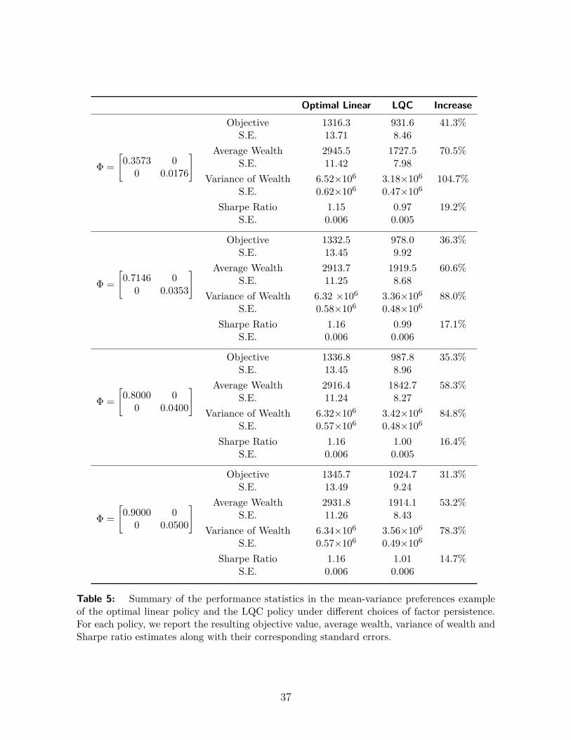
Optimal Linear LQC Increase

Φ =[0.3573 0

0 0.0176

]Objective 1316.3 931.6 41.3%

S.E. 13.71 8.46Average Wealth 2945.5 1727.5 70.5%

S.E. 11.42 7.98Variance of Wealth 6.52×106 3.18×106 104.7%

S.E. 0.62×106 0.47×106

Sharpe Ratio 1.15 0.97 19.2%S.E. 0.006 0.005

Φ =[0.7146 0

0 0.0353

]Objective 1332.5 978.0 36.3%

S.E. 13.45 9.92Average Wealth 2913.7 1919.5 60.6%

S.E. 11.25 8.68Variance of Wealth 6.32 ×106 3.36×106 88.0%

S.E. 0.58×106 0.48×106

Sharpe Ratio 1.16 0.99 17.1%S.E. 0.006 0.006

Φ =[0.8000 0

0 0.0400

]Objective 1336.8 987.8 35.3%

S.E. 13.45 8.96Average Wealth 2916.4 1842.7 58.3%

S.E. 11.24 8.27Variance of Wealth 6.32×106 3.42×106 84.8%

S.E. 0.57×106 0.48×106

Sharpe Ratio 1.16 1.00 16.4%S.E. 0.006 0.005

Φ =[0.9000 0

0 0.0500

]Objective 1345.7 1024.7 31.3%

S.E. 13.49 9.24Average Wealth 2931.8 1914.1 53.2%

S.E. 11.26 8.43Variance of Wealth 6.34×106 3.56×106 78.3%

S.E. 0.57×106 0.49×106

Sharpe Ratio 1.16 1.01 14.7%S.E. 0.006 0.006

Table 5: Summary of the performance statistics in the mean-variance preferences exampleof the optimal linear policy and the LQC policy under different choices of factor persistence.For each policy, we report the resulting objective value, average wealth, variance of wealth andSharpe ratio estimates along with their corresponding standard errors.

37

S. Basak and G. Chabakauri. Dynamic mean-variance asset allocation. Review of Financial Studies,23(8):2970–3016, 2010. doi: 10.1093/rfs/hhq028.

A. Ben-Tal, A. Goryashko, E. Guslitzer, and A. Nemirovski. Adjustable robust solutions of uncer-tain linear programs. Mathematical Programming, 99(2):351–376, 2004.

A. Ben-Tal, B. Golany, A. Nemirovski, and J. Vial. Retailer-supplier flexible commitments con-tracts: A robust optimization approach. Manufacturing & Service Operations Management, 7:248–271, July 2005.

D. P. Bertsekas. Dynamic Programming and Optimal Control. Athena Scientific, 2nd edition, 2000.ISBN 1886529094.

D. Bertsimas and V. Goyal. On the power and limitations of affine policies in two-stage adaptiveoptimization. Mathematical Programming, pages 1–41, 2011.

D. Bertsimas and A. Lo. Optimal control of execution costs. Journal of Financial Markets, 1(1):1–50, 1998. ISSN 1386-4181.

D. Bertsimas, D. A. Iancu, and P. A. Parrilo. Optimality of affine policies in multistage robustoptimization. Math. Oper. Res., 35, May 2010.

S. Boyd and L. Vandenberghe. Convex Optimization. Cambridge University Press, March 2004.ISBN 0521833787.

S. Boyd, M. T. Mueller, B. O’Donoghue, and Wang Y. Performance bounds and suboptimal policiesfor multi-period investment. Working paper, 2012.

M. W. Brandt and P. Santa-Clara. Dynamic portfolio selection by augmenting the asset space. TheJournal of Finance, 61(5):2187–2217, 2006.

M. W. Brandt, A. Goyal, P. Santa-Clara, and J. R. Stroud. A simulation approach to dynamicportfolio choice with an application to learning about return predictability. Review of FinancialStudies, 18(3):831–873, 2005.

M. W. Brandt, P. Santa-Clara, and R. Valkanov. Parametric portfolio policies: Exploiting char-acteristics in the cross-section of equity returns. Review of Financial Studies, 22(9):3411–3447,September 2009.

D. B. Brown and J. E. Smith. Dynamic portfolio optimization with transaction costs: Heuristicsand dual bounds. Working paper, 2010.

G. C. Calafiore. An affine control method for optimal dynamic asset allocation with transactioncosts. SIAM J. Control Optim., 48:2254–2274, June 2009.

J. Y. Campbell and L. M. Viceira. Strategic asset allocation. Oxford University Press Oxford, 2002.

N. Chen, R. Roll, and S. A. Ross. Economic forces and the stock market. The Journal of Business,59(3):pp. 383–403, 1986.

X. Chen, M. Sim, and P. Sun. A robust optimization perspective on stochastic programming.Operations Research, 55:1058–1071, November 2007.

38

X. Chen, M. Sim, P. Sun, and J. Zhang. A linear decision-based approximation approach tostochastic programming. Operations Research, 56:344–357, March 2008.

G. M. Constantinides. Capital market equilibrium with transaction costs. The Journal of PoliticalEconomy, 94(4):pp. 842–862, August 1986.

J. Cvitanic. Theory of portfolio optimization in markets with frictions. In E. Jouini, J. Cvitanic,and Marek Musiela, editors, Handbooks in Mathematical Finance. Cambridge University Press,2001.

M. H. A. Davis and A. R. Norman. Portfolio selection with transaction costs. Mathematics ofOperations Research, 15(4):676–713, 1990.

V. V. Desai, V. F. Farias, and C. C. Moallemi. Pathwise optimization for linear convex systems.Working paper, 2011.

J. B. Detemple, R. Garcia, and M. Rindisbacher. A Monte Carlo method for optimal portfolios.The Journal of Finance, 58(1):401–446, February 2003.

B. Dumas and E. Luciano. An exact solution to a dynamic portfolio choice problem under trans-actions costs. The Journal of Finance, 46(2):pp. 577–595, 1991.

E. F. Fama and K. R. French. Multifactor explanations of asset pricing anomalies. The Journal ofFinance, 51(1):pp. 55–84, 1996.

N. Gârleanu and L. H. Pedersen. Dynamic trading with predictable returns and transaction costs.The Journal of Finance, 68(6):2309–2340, 2013.

J. Gatheral. No-dynamic-arbitrage and market impact. Quantitative Finance, 10(7):749–759, 2010.

P. Glasserman and X. Xu. Robust portfolio control with stochastic factor dynamics. Workingpaper, 2011.

W. N. Goetzmann and P. Jorion. Testing the predictive power of dividend yields. Journal ofFinance, 48(2):663–679, 1993.

M. Grant and S. Boyd. CVX: Matlab software for disciplined convex programming, version 1.21.http://cvxr.com/cvx, April 2011.

R. C. Grinold and R. N. Kahn. Active Portfolio Management. McGraw-Hill, 2nd edition, 1999.

S. J. Grossman and Z. Zhou. Optimal investment strategies for controlling drawdowns. Mathemat-ical Finance, 3(3):241–276, 1993.

S. L. Heston, R. A. Korajczyk, and R. Sadka. Intraday patterns in the cross-section of stock returns.Journal of Finance, 65(4):1369–1407, 2010.

M. Hora. Tactical liquidity trading and intraday volume. Working Paper, 2006.

D. Kuhn, W. Wiesemann, and A. Georghiou. Primal and dual linear decision rules in stochasticand robust optimization. Mathematical Programming, pages 1–33, 2009.

39

H. Liu. Optimal consumption and investment with transaction costs and multiple risky assets.Journal of Finance, 59(1):289–338, 02 2004.

H. Liu and M. Loewenstein. Optimal portfolio selection with transaction costs and finite horizons.Review of Financial Studies, 15(3):805–835, 2002.

A. W. Lynch and P. Balduzzi. Predictability and transaction costs: The impact on rebalancingrules and behavior. Journal of Finance, 55(5):2285–2309, October 2000.

A. W. Lynch and S. Tan. Multiple risky assets, transaction costs, and return predictability: Allo-cation rules and implications for U.S. investors. Journal of Financial and Quantitative Analysis,45(04):1015–1053, August 2010.

Robert C. Merton. Optimum consumption and portfolio rules in a continuous-time model. Journalof Economic Theory, 3(4):373–413, December 1971.

A. Nemirovski, A. Juditsky, G. Lan, and A. Shapiro. Stochastic approximation approach to stochas-tic programming. SIAM Journal on Optimization, 19(4):1574–1609, 2009.

A. A. Obizhaeva and J. Wang. Optimal trading strategy and supply/demand dynamics. Workingpaper, 2005.

A. Shapiro. Monte Carlo sampling methods. In A. Ruszczynski and A. Shapiro, editors, StochasticProgramming, volume 10 of Handbooks in Operations Research and Management Science, pages353 – 425. Elsevier, 2003.

A. Shapiro and A. Nemirovski. On complexity of stochastic programming problems. In Panos M.Pardalos, Donald Hearn, Vaithilingam Jeyakumar, and Alexander Rubinov, editors, ContinuousOptimization, volume 99 of Applied Optimization, pages 111–146. Springer, 2005.

S. E. Shreve and H. M. Soner. Optimal investment and consumption with transaction costs. TheAnnals of Applied Probability, 4(3):pp. 609–692, 1994.

J. Skaf and S. P. Boyd. Nonlinear Q-design for convex stochastic control. IEEE Transactions onAutomatic Control, 54(10):2426–2430x, October 2009.

J. Skaf and S. P. Boyd. Design of affine controllers via convex optimization. IEEE Transactionson Automatic Control, 55(11):2476–2487, November 2010.

40

Technical Appendices

A. Efficient Exact Formulations

In this section, we will provide efficient exact formulations of dynamic portfolio choice prob-

lems using the class of linear policies for our feasible set of policies. In particular, we will

consider a number of the examples of dynamic portfolio choice problems discussed in Sec-

tion 2.1. These examples include features such as constraints on portfolio holdings, trans-

action costs, and risk measures. In each case, we will demonstrate how the optimization

problem (11) can be transformed into a deterministic convex program by explicit analytical

evaluation of the objective function E[p(·, f)] and the constraint set C.

Exact formulations require the evaluation of expectations taken over the sample path of

factor realizations f . In order to do this, we will make the following assumption for the rest

of this section:

Assumption 4 (Gaussian factors). Assume that the sample path f of factor realizations is

jointly Gaussian. In particular, denote by Ft , (f1, . . . , ft)> ∈ RKt the vector of all factors

observed by time t. We assume that Ft ∼ N(θt,Ωt), where θt ∈ RKt is the mean vector and

Ωt ∈ RKt×Kt is the covariance matrix.

Note that this assumption is not necessary for the practical application of our method.

Indeed, as discussed in Section 3, sample average approximation or stochastic approximation

methods can be used to determine the optimal policy in the absence of such an assumption.

However, under Assumption 4, the optimal linear policy can be solved via a determinis-

tic convex optimization program that does not involve any sampling. This is often more

computationally efficient as well as more accurate (since there are no errors introduced by

sampling).

With this assumption, the trades of any linear policy will also be jointly normally dis-

41

tributed, as each such policy is affine transformations of the factors. Formally, let

(29) Mt ,[E1,t E2,t . . . Et,t

]∈ RN×Kt

be the matrix of time t policy coefficients, so that the trade vector is given by ut = ct+MtFt.

With this representation, it is easy to see that ut ∼ N(ut, Vt), where the mean vector and

covariance matrix are given by

ut , E[ut] = ct +Mtθt, Vt , Var(ut) = MtΩtM>t .(30)

Similarly, the portfolio xt at time t is normally distributed. we have that

(31) xt = x0 +t∑i=1

ui = x0 +t∑i=1

(ci +

i∑s=1

Es,ifs

)= dt +

t∑s=1

Js,tfs,

where dt , x0 + ∑ti=1 ci and Js,t ,

∑t`=sEs,`. With this representation, it is easy see that

xt ∼ N(κt, Yt), where

κt , E[xt] = dt + Ptθt, Yt , Var(xt) = PtΩtP>t ,(32)

Pt ,[J1,t J2,t . . . Jt,t

].(33)

A.1. Linear Constraints

We will provide formulations for linear equality or inequality constraints on trades or po-

sitions, in the context of linear rebalancing policies. These types of constraints appear

frequently in portfolio choice due to regulatory reasons such as short sale restriction, liqui-

dation purposes or diversification needs (e.g., keeping a specific industry exposure under a

certain limit).

42

A.1.1. Equality Constraints

Equality constraints appear often in portfolio choice, particularly in portfolio execution prob-

lems when the investor needs to liquidate a certain portfolio (i.e., xT = 0) or constructs a

certain target portfolio by the end of the time horizon (i.e., xT = x).

Suppose that for some time t, we have a linear equality constraint on the trade vector

ut, of the form Aut = b. Here, A ∈ RM×N and b ∈ RN . This constraint can be written as

(34) Act + AMtFt = b.

Under Assumption 4, the left side of (34) is normally distributed. Therefore, for (34) to

hold almost surely, we must have that the left side has mean b and zero covariance. Thus,

we require that

Act = b, AMt = 0.(35)

Thus, the linear equality constraint (34) on the trade vector ut is equivalent to the linear

equality constraint (35) on the policy coefficients (ct,Mt). Linear equality constraints on the

portfolio position xt can be handled similarly.

A.1.2. Inequality Constraints

Inequality constraints on trades or positions are common as well. One example is a short-sale

constraint, which would require that xt ≥ 0 for all times t. When the factor realizations do

not have bounded support, inequality constraints cannot be enforced almost surely. This is

true in the Gaussian case: there is a chance, however small, that factors may take extreme

values, and if the policy is a linear function of the factors, this may cause an inequality

constraint to be violated. In other words, under Assumption 4 with linear constraints, any

non-deterministic linear rebalancing policy will typically be infeasible. Note that while this

43

is immediate in the exact formulation, this difficulty remains if we employ other solution

methods such as sample average approximation. In the SAA approach, for example, any

non-deterministic linear rebalance policy will become infeasible given enough samples.

In order to account for such constraints in a linear rebalancing policy, instead of enforcing

inequality constraints almost surely, we will enforce them at a given level of confidence. For

example, given a vector a ∈ RN and a scalar b, instead of enforcing the linear constraint

a>ut ≤ b, almost surely, we can consider a relaxation where we seek to guarantee that it

is violated with small probability. In other words, we can impose the chance constraint

P(a>ut > b) ≤ η, for a small value of the parameter η. The following lemma illustrates that

this can be accomplished explicitly:

Lemma 1. Given η ∈ [0, 1/2], a non-zero vector a ∈ RN , and a scalar b, the chance constraint

P(a>ut > b) ≤ η is equivalent to the constraint

a> (ct +Mtθt)− b+ Φ−1(1− η)∣∣∣∣∣∣Ω1/2

t M>t a∣∣∣∣∣∣

2≤ 0

on the policy coefficients (ct,Mt), where Φ−1(·) is the inverse cumulative normal distribution.

Proof. This proof follows standard arguments in convex optimization (see, e.g., Boyd and

Vandenberghe, 2004). Let ut and Vt be the mean and the variance of ut as given in (30).

Then,

P(a>ut > b) = P(βt + σtZ > 0),

where

βt , a>ut − b, σt , ‖V 1/2t a‖2 6= 0,

and Z is a standard normal random variable. Thus,

P(a>ut > b) = 1− Φ(−βt/σt).

44

Note that the this probability is less than or equal to η if and only if

βt + Φ−1(1− η)σt ≤ 0.

Substituting (30) into definitions for βt and σt, we obtain the desired result.

A similar approach can be applied to incorporate linear inequality constraints on the

portfolio position xt with high confidence.

In many situations (e.g., short-sale constraints), it may not be sufficient to enforce an

inequality constraint only probabilistically. In such cases, when a linear rebalancing policy

is applied, the resulting trades can be projected onto the constraint set so as to ensure that

the constraints are always satisfied. When the linear policy is designed, however, it is helpful

to incorporate the desired constraints probabilistically so as to account for their presence.

We will demonstrate this idea in the application in Section 4.

A.2. Transaction Costs

In this section, we will provide efficient exact formulations for the transaction cost functions

discussed in Section 2.1, in the context of linear rebalancing policies. In general, one might

consider a total transaction cost of

TC(u) ,T∑t=1

TCt(ut)

for executing the sample path of trades u, where TCt(ut) is the cost of executing the trade

vector ut at time t. As seen in Section 2.1, we typically wish to subtract an expected trans-

action cost term from investor’s objective. Hence efficient exact formulations for transaction

costs involve explicit analytical computation of E[TC(u)] = ∑Tt=1 E[TCt(ut)], when each trade

vector ut is specified by a linear policy.

Under a linear policy, ut ∼ N(ut, Vt) is distributed as a normal random variable with

45

mean and covariance, (ut, Vt), specified with the policy coefficients, (E, c), through (30).

Then, the evaluation of expected transaction costs reduces to the evaluation of the expected

value of the per-period transaction cost function TCt(·) for a Gaussian random variable. This

can be handled on a case-by-case basis as follows:

• Quadratic transaction costs. In the case of quadratic transaction costs, as seen in Ex-

ample 2, the per period transaction cost function is given by TCt(ut) , 12u>t Λut, where

Λ ∈ RN×N is a positive definite matrix. In this case, E[TCt(ut)] = 12 (utΛut + tr(ΛVt)) .

• Proportional transaction costs. In the case of proportional transaction costs, as

discussed in Example 4, the per period transaction cost function is given by

TCt(ut) ,N∑i=1

χi|ut,i|,

where χi > 0 is a proportionality constant specific to security i. Using the properties

of the folded normal distribution, we obtain

E[TCt(ut)] =N∑i=1

χi

√2Vt,iπ

exp−u2t,i

2Vt,i

+ ut,i

1− 2Φ− ut,i√

Vt,i

,

where Φ(·) is the cumulative distribution function of a standard normal random vari-

able.

• Nonlinear transaction costs. In the case of nonlinear transaction costs, as discussed

in Example 4, the per period transaction cost function is given by

TCt(ut) ,N∑i=1

χi|ut,i|β,

where χi > 0 is a proportionality constant specific to security i, and β ≥ 1 is an

exponent capturing the degree of nonlinearity. As in the proportional case, evaluating

46

the Gaussian expectation explicitly results in

E[TCt(ut)] =N∑i=1

χiΓ(

1 + β

2

)(2Vt,i)

β2

√π

1F1

(−β2 ; 1

2;−u2t,i

2Vt,i

),

where Γ(·) is the gamma function and 1F1(·) is the confluent hypergeometric function

of the first kind.

A.3. Terminal Wealth and Risk Aversion

In many of the portfolio choice examples in Section 2.1, an investor wishes to maximize

expected wealth net of transaction costs, subject to a penalty for risk, i.e.,

(36) maximizeπ∈UF

Eπ[W (x, r)− TC(u)− RA(x, f , r)

)].

Here, W (·) is the terminal wealth associated with a sample path, TC(·) are the transaction

costs, and RA(·) is a penalty for risk aversions. Exact calculation of expected transaction

costs for linear policies were discussed in Section A.2. Here, we will discuss exact calculation

of the expected terminal wealth and the risk aversion penalty.

To begin, note that the terminal wealth depends on realized returns in addition to factor

realizations. Hence, we will make the following assumption:

Assumption 5 (Gaussian returns). As in Example 2, assume that for each time t ≥ 0, returns

evolve according to

(37) rt+1 = µt +Bft + ε(2)t+1,

where µt is a deterministic vector, B is a matrix of factor loadings, and ε(2)t are zero-mean

i.i.d. Gaussian disturbances with covariance Σ.

Note that the critical assumption we are making here is that the factor realizations f

47

and the sample path of security returns r are jointly Gaussian. The particular form (37) is

chosen out of convenience but is not necessary.

We can calculate the expected terminal wealth as

E[W (x, r)] = W0 +T∑t=1

E[x>t rt+1] = W0 +T∑t=1

(µ>t κt + E[x>t Bft]

),

= W0 +T∑t=1

(µ>t κt + d>t Bδt +

t∑s=1

(δ>s (B(I − Φ)t−sJ>s,t)δs + tr

(B(I − Φ)t−sJ>s,tωs

))),

where ωs is the sth K ×K diagonal block matrix of Ωt.

For the risk aversion penalty, we consider two cases:

• Per period risk penalty. Consider risk aversion penalties that decompose over time as

RA(x, f , r) =N∑t=1

RAt(xt),

where RAt(·) is a function which penalizes for risk aversion based on the positions held

at time t. One such case is the quadratic penalty RAt(xt) , γ2x>t Σxt of Example 2,

where γ > 0 is a risk penalty proportionality constant. Here, the investor seeks to

penalize in proportion to the conditional per period variance of the portfolio value. So

long as the expectation of RAt(·) can be calculated for Gaussian arguments, then the

overall expected risk aversion penalty can be calculated exactly. This can be accom-

plished for a variety of functions. For example, quadratic penalties can be handled in

a manner analogous to the quadratic transaction costs discussed in Section A.2.

• Terminal wealth risk penalty. Alternatively, as discussed in Example 5, a more natural

risk aversion criteria might be to penalize risk as a function of the terminal wealth.

Specifically, an investor with mean-variance preferences would consider a risk aversion

penalty RA(x, f , r) , −γ2 Var(W (x, r)), where γ > 0 is a risk penalty proportionality

constant.

Following the notation of Section A, we will compute Var[W (x, r)] analytically and

48

demonstrate that the resulting expression is a quadratic convex function of the policy

coefficients. Without loss of generality, assume that W0 = 0 and µt = 0. Let d ∈

RNT×1, e ∈ RNT×1, L ∈ RNT×KT , and D ∈ RNT×KT with

d ,

d1

d2

...

dT−1

dT

, e ,

ε(2)1

ε(2)2...

ε(2)T−1

ε(2)T

, L ,

B 0 . . . 0 0

0 B . . . 0... . . . . . . 0

. . . B 0

0 . . . 0 B

,

D ,

J1,1 0 . . . 0 0

J1,2 J2,2 . . . 0... . . . . . . 0

. . . . . . 0

J1,T . . . JT−1,T JT,T

.

Then, observe that[x>1 . . . x>T

]>= d+DFT , and W (x, r) = (d+DFT )> (LFT + e).

Using the independence between e and FT and E[e] = 0, we obtain

Var (W (x, r)) = E[(d+DFT )> (LFT + e)(LFT + e)> (d+DFT )

]− E

[(d+DFT )> (LFT + e)

]2= E

[(d+DFT )> ee> (d+DFT )

]+ E

[(d+DFT )> (LFT )(LFT )> (d+DFT )

]− E

[(d+DFT )> (LFT )

]2

(38)

We need the following fact from multivariate statistics in order to compute the expec-

tations.

Fact 1. If z is a random vector with mean m and variance S, and Q, A, H are constant

49

matrices, and a is a constant vector, then

E[z>Qz

]= tr(QS) +m>Qm,

E[(Az + a)>Hz(Hz)>(Az + a)

]= tr

(AS(H>A+ A>H)SH>

)+((Am+ a)>H + (Hm)>A

)S((Am+ a)>H + (Hm)>A

)>+(tr(ASH>

)+ (Am+ a)>Hm

)2.

We will consider each of the three terms in (38) separately. The first expectation,

E[(d+DFT )> ee> (d+DFT )

], can be evaluated using the independence of ε(2)

s and

ε(2)t when s 6= t and Fact 1.

E[(d+DFT )> ee> (d+DFT )

]=

T∑t=1

E[x>t E

[ε

(2)t+1

(ε

(2)t+1

)>|Ft]xt

]

=T∑t=1

E[x>t Σxt

]

=T∑t=1

(dt + Ptθt)>Σ (dt + Ptθt) + tr(ΣPtΩtP

>t

).

Note that this term is equivalent to the sum of per-period risk penalties considered in

the previous section.

The remaining expectations in (38) can be directly computed using Fact 1 with replac-

ing z with FT where FT ∼ N(ΘT ,ΩT ).

E[(d+DFT )> (LFT )(LFT )> (d+DFT )

]= tr

(DΩT (L>D +D>L)ΩTL

>)

+((DΘT + d)>L+ (LΘT )>D

)ΩT

((DΘT + d)>L+ (LΘT )>D

)>+(tr(DΩTL

>)

+ (DΘT + d)> LΘT

)2.

50

Finally,

E[(d+DFT )> (LFT )

]2=(tr(DΩTL

>)

+ (DΘT + d)> LΘT

)2.

Summing all three terms in (38), we obtain the exact expression for the variance of

terminal wealth:

Var (W (x, r)) =T∑t=1

(dt + Ptθt)>Σ (dt + Ptθt) + tr(ΣPtΩtP

>t

)+ tr

(DΩT (L>D +D>L)ΩTL

>)

+((DΘT + d)>L+ (LΘT )>D

)ΩT

((DΘT + d)>L+ (LΘT )>D

)>.

(39)

Note that this expression is convex in our decision variables, as expected.

B. Derivation of the LQC Policies

We can derive a closed-form solution for our trading policy when the problem satisfies the

LQC framework. We guess a functional form for the value function and show that this

functional form is preserved at each time step.

Using dynamic programming principle and ut = (xt−xt−1), the value function Vt(xt−1, ft)

satisfies

Vt−1(xt−1, ft) = maximizext

(x>t (Bft)−

12(xt − xt−1)>Λ(xt − xt−1) + E[Vt(xt, ft+1)]

).

We guess the following quadratic form for our value function:

Vt(xt, ft+1) = −12x>t Axx,txt + x>t Axf,tft+1 + 1

2f>t+1Aff,tft+1 + 1

2mt.

51

Then,

E[Vt(xt, ft+1)] = −12x>t Axx,txt+x>t Axf,t (I − Φ) ft+

12f>t (I − Φ)>Aff,t (I − Φ) ft+

12 (tr(ΨAff,t) +mt) .

At the last period, we need xT = 0, and our value function equals

VT−1(xT−1, ft) = −12x>T−1ΛxT−1

which satisfies our functional form with

Axx,T−1 = Λ Axf,T−1 = 0 Aff,T−1 = 0 mT−1 = 0.

For all t < T − 1, we maximize the quadratic objective −12x>t Qtxt + x>t qt + bt where

Qt = Λ + Axx,t

qt = Λxt−1 + (B + Axf,t (I − Φ)) ft

bt = −12x>t−1Λxt−1 + 1

2f>t (I − Φ)>Aff,t (I − Φ) ft + tr(ΨAff,t) +mt

Then, the optimal xt is given by Q−1t qt and xt and ut are given by

xt = (Λ + Axx,t)−1 (Λxt−1 + (B + Axf,t (I − Φ)) ft)

ut = (Λ + Axx,t)−1 (Λxt−1 + (B + Axf,t (I − Φ)) ft)− xt−1

52

The maximum then occurs at 12q>t Q−1t qt + bt and we obtain the following recursions:

Axx,t−1 = −Λ (Λ + Axx,t)−1 Λ + Λ

Axf,t−1 = Λ (Λ + Axx,t)−1 (B + Axf,t (I − Φ))

Aff,t−1 = (B + Axf,t (I − Φ))> (Λ + Axx,t)−1 (B + Axf,t (I − Φ)) + (I − Φ)>Aff,t (I − Φ)

mt−1 = tr(ΨAff,t) +mt

Using these recursions, we can compute the optimal expected payoff of the dynamic

program. Using f0 = N(0,Ω0),

E[V0(x0, f1)] = E [E[V0(x0, f1)|f0]]

= E[−1

2x>0 Axx,0x0 + x>0 Axf,0 (I − Φ) f0 + 1

2f>0 (I − Φ)>Aff,0 (I − Φ) f0 + 1

2 (tr(Ω0Aff,0) +m0)]

= −12x>0 Axx,0x0 + 1

2

(tr(Ω0(I − Φ)>Aff,0(I − Φ)

)+

T−2∑t=0

tr(ΨAff,0)).

C. Exact Formulation of Best Linear Execution Policy

We will first compute the expectation in the objective of (21) and write the equivalent deter-

ministic form. We will then replace probabilistic constraints with deterministic constraints

using Lemma 1, and finally obtain the deterministic version of the stochastic program in

(21).

We start working with the expectation in the objective function. For each t, we have to

compute the expectation of the following two terms, E[x>t (Bft)

], and E

[u>t Λut

]. First, we

derive the statistics for ft, ut and xt. We first note that

ft = (I − Φ)T e0 +t∑

s=1(I − Φ)t−sε(1)

s .

53

Letting Ft , (f1, . . . , ft)>, Then, in vector form, we have the following representation

Ft =

(I − Φ)f0

(I − Φ)2f0

...

(I − Φ)t−1f0

(I − Φ)tf0

+

I 0 . . . 0 0

(I − Φ) I 0 . . . 0... (I − Φ) . . . . . . 0

(I − Φ)t−1 . . .. . . I 0

(I − Φ)t . . . (I − Φ) I

︸ ︷︷ ︸

,At

ε(1)1

ε(1)2...

ε(1)t−1

ε(1)t

.

Using this representation, we compute the mean

(40) θt , E[Ft] =

δ1

δ2

...

δt−1

δt

,

(I − Φ)f0

(I − Φ)2f0

...

(I − Φ)t−1f0

(I − Φ)tf0

,

and the covariance matrix

(41) Ωt , Var[Ft] = At

Ψ 0 . . . 0 0

0 Ψ . . . 0... . . . . . . 0

. . . Ψ 0

0 . . . 0 Ψ

A>t .

Note that Ωt is a block diagonal matrix with t blocks of size K ×K. Recall that in Section

A, we defined

(42) Mt ,[E1,t E2,t . . . Et,t

]

54

Then, ut = ct +MtFt and we have the following moments for ut:

µt , E[ut] = ct +Mtθt(43)

Vt , Var(ut) = MtΩtM>t .

Therefore, ut is normally distributed with mean µt and covariance matrix Vt. Similarly, we

can obtain the statistics for xt. Using (32),

κt , E[xt] = dt + Ptθt

Yt , Var(xt) = PtΩtP>t .

Using Fact 1, we can compute each term in the expectation.

E[x>t (Bft)

]= E

[d>t Bft +

t∑s=1

f>s J>s,tBft

]

= d>t Bδt +t∑

s=1E[f>s J

>s,tBE [ft|fs]

]

= d>t Bδt +t∑

s=1E[f>s J

>s,tB(I − Φ)t−sfs

]

= d>t Bδt +t∑

s=1

(δ>s (B(I − Φ)t−sJ>s,t)δs + tr

(B(I − Φ)t−sJ>s,tωs

))

where ωs is the sth diagonal block matrix of Ωt having a size of K × K. Finally, for the

transaction cost terms,

E[u>t Λut

]= E

[(ct +MtFt)> Λ (ct +MtFt)

]= (ct +Mtθt)> Λ (ct +Mtθt) + tr

(ΛMtΩtM

>t

)

55

Summing up all the terms, our final objective function in deterministic form equals

maximizect,Es,t

T∑t=1

d>t Bδt +

t∑s=1

(δ>s (B(I − Φ)t−sJ>s,t)δs + tr

(B(I − Φ)t−sE>s,tωs

))+ 1

2((ct +Mtθt)> Λ (ct +Mtθt) + tr

(ΛMtΩtM

>t

)),

which is a quadratic function of the policy parameters.

We now rewrite the equality constraint, xT = 0 in terms of policy parameters. In order

to enforce this equality, we need

dT = 0 and Js,T = 0 s = 1, . . . , T.

Lastly, we replace probabilistic constraints with deterministic constraints using Lemma 1.

Note that P (xt ≤ 0) ≤ η can be written as P (−xt ≥ 0) ≤ η. Then, using Lemma 1,

(−dt − Ptθt) + Φ−1(1− η)∣∣∣∣∣∣∣∣(PtΩtP

>t

)1/2∣∣∣∣∣∣∣∣

2≤ 0.

Similarly, we obtain that P (ut ≥ 0) ≤ η can be replaced by

(ct +Mtθt) + Φ−1(1− η)∣∣∣∣∣∣∣∣(MtΩtM

>t

)1/2∣∣∣∣∣∣∣∣

2≤ 0.

Combining all the results, we obtain the deterministic version of the stochastic program

in (21), a second-order cone program:

56

maximizect,Es,t

T∑t=1

d>t Bδt +t∑

s=1

(δ>s (B(I − Φ)t−sJ>s,t)δs + tr

(B(I − Φ)t−sE>s,tωs

))(44)

+ 12((ct +Mtθt)> Λ (ct +Mtθt) + tr

(M>

t ΛMtΩt

))subject to dt = x0 +

t∑i=1

ci t = 1, . . . , T,

Js,t =t∑i=s

Es,i 1 ≤ s ≤ t ≤ T,

(−dt − Ptθt) + Φ−1(1− η)∣∣∣∣∣∣∣∣(PtΩtP

>t

)1/2∣∣∣∣∣∣∣∣

2≤ 0 t = 1, . . . , T,

(ct +Mtθt) + Φ−1(1− η)∣∣∣∣∣∣∣∣(MtΩtM

>t

)1/2∣∣∣∣∣∣∣∣

2≤ 0 t = 1, . . . , T,

dT = 0 and Js,T = 0.

Note that the number of decision variables is greater than that of the original execution

problem in (16). Total number of decision variables in a problem with N securities, K factors

and T periods equals 2NT +NKT (T + 1) which is on the order of O(NKT 2).

57