dynamic portfolio optimisationan example of a hedging portfolio 4 • assume returns, r, in any...

Dynamic Portfolio OptimisationJames Sefton

July 2007

What new questions does dynamic optimisation address?

1

• Assume a manager has two strategies:

1. The first strategy has a high return but decays quickly.

2. The second has a lower expected return but decays more slowly.

How should the manager use this information in constructing his portfolio?

• Now take into account transaction costs and problem becomes interesting!

• Multiperiod optimisation introduces hedging motives for holding some assets. These asset hedge against future falls in expected returns in the strategies (or the future investment opportunity set).

Diversification of within period risk

2

-0.1

0

0.1

0.2

0.3

1 2 3 4 5 6 7 8 9 10

Asset 1 Asset 2 Portfolio

• Construct a portfolio from two assets that are negatively correlated in each period. Within period variance is less than the variance of each asset.

• The distribution of the return histories over n periods has mean and variance equal to ntimes the within period mean and variance.

Distribution of Return Histories

0 0.2 0.4 0.6 0.8 1 1.2 1.4 1.6 1.8 20

0.5

1

1.5

2

2.5

Time diversification of risk

3

0 0.2 0.4 0.6 0.8 1 1.2 1.4 1.6 1.8 20

0.5

1

1.5

2

2.5

3-0.1

0

0.1

0.2

0.3

1 2 3 4 5 6 7 8 9 10

Portfolio Hedge Hedged Portfolio

• Construct a hedged portfolio from earlier portfolio and a hedge where hedge is negatively correlated to portfolio acrossperiods. Within period variance can be greater than the variance of unhedged portfolio.

• But the distribution of the return histories over n periods has mean and variance less than ntimes the within period mean and variance.

Distribution of Return Histories

An example of a Hedging Portfolio

4

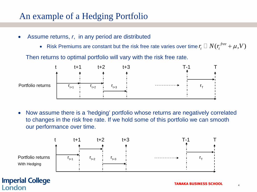
• Assume returns, r, in any period are distributed • Risk Premiums are constant but the risk free rate varies over time

Then returns to optimal portfolio will vary with the risk free rate.

• Now assume there is a ‘hedging’ portfolio whose returns are negatively correlated to changes in the risk free rate. If we hold some of this portfolio we can smooth our performance over time.

( , )freet tr N r Vµ+

t t+1 t+2 t+3 T-1 T

Portfolio returns rt+1 rt+2 rt+3 rT

t t+1 t+2 t+3 T-1 T

Portfolio returns rt+1 rt+2 rt+3 rT

With Hedging

Return Predictability and Transaction Costs can induce correlation across periods

5

Time t t+1 t+2Portfolio weights wt wt+1

Portfolio returns wt rt+1- (wt+1 –wt )2T wt+1 rt+2

Time t t+1 t+2Portfolio weights wt wt+1

Portfolio returns wt rt+1- (wt+1 –wt )2T wt+1 rt+2

Transaction Costs

( ) ( )( )

1 2 1 1

1 1 for 1,2t t t t t

t i t i t i t

r r

r r i

ξ

ε+ + + +

+ + − + +

= Α +

= + =

E E

E

• Let denote expected returns at the beginning of the period. Let the portfolio construction rule be and define the system equations as follows

where ξ, ε are i.i.d. random variables.

• Note the following

1. Returns are just equal to expected returns plus an innovation.

2. Expected returns are time-varying if ξ≠0 and predictable if A≠ 0.

3. The portfolio rule can be any function of expected returns – this is just the simplest.

4. Transaction cost can be any function of the change in portfolio weights.

( )1e

t i t i t ir E r+ + − +=

2 1 1

1 for 1,2

e et t t

et i t i t

r Ar

r r i

ξ

ε+ + +

+ + +

= +

= + =

1e

t tw Kr +=

Return Predictability and Transaction Costs can induce correlation across periods

6

( ) ( )( )( ) ( )

1 2 1 1

1 1 1

2 1 2 2 1 1 2

t t t t t

t t t t

t t t t t t t t

r r

r r

r r r

ξ

ε

ε ξ ε

+ + + +

+ + +

+ + + + + + +

= Α +

= +

= + = Α + +

E E

E

E E

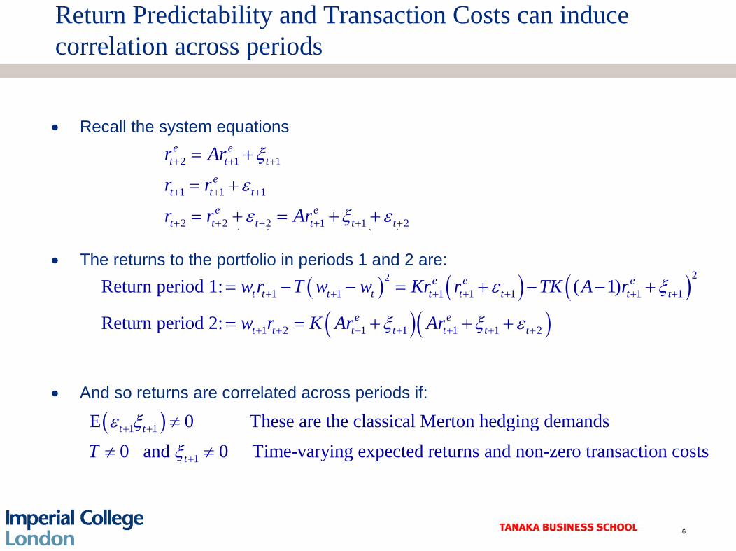
• Recall the system equations

• The returns to the portfolio in periods 1 and 2 are:

• And so returns are correlated across periods if:

( ) ( ) ( )( )( )

221 1 1 1 1 1 1

1 2 1 1 1 1 2

Return period 1: ( 1)

Return period 2:

e e et t t t t t t t t

e et t t t t t t

w r T w w Kr r TK A r

w r K Ar Ar

ε ξ

ξ ξ ε

+ + + + + + +

+ + + + + + +

= − − = + − − +

= = + + +

( )1 1

1

E 0 These are the classical Merton hedging demands0 and 0 Time-varying expected returns and non-zero transaction costt t

tTε ξ

ξ+ +

+

≠

≠ ≠

2 1 1

1 1 1

2 2 2 1 1 2

e et t t

et t t

e et t t t t t

r Ar

r r

r r Ar

ξ

ε

ε ξ ε

+ + +

+ + +

+ + + + + +

= +

= +

= + = + +

s

The Dynamic Portfolio Construction Problem

7

• The problem is to choose portfolios, wt, to maximise the performance measure

• This is just mean-variance extended to the multi-period problem. For if

( )1 11 log t TE W g

g-

-é ùê úë û

Time t t+1 t+2 T-1 T

Wealth Wt Wt+1 W t+2 WT-1 WT

Portfolio weights wt wt+1 w t+2 wT-1 wT

Stock returns rt+1 rt+2 rT

Portfolio returns wt rt+1 wt+1rt+2 wT-1rT

Condition. Vars. st st+1 s t+2 sT-1 sT


Wealth Wt Wt+1 W t+2 WT-1 WT




Condition. Vars. st st+1 s t+2 sT-1 sT

( )1 111 2

(1+ r) then

log log ( ) ( )

rT t t

t T t

W W e W

E W W E r V ar rggg

---

= »

= + +

A Tractable Optimisation Criterion

8

• We use Campbell & Viceria (2003) log-linear approximation. Let Var(rt)=Σ and σ2=diag(Σ )

• And substitute this into our performance measure

• This is an exponential of a quadratic cost or risk-sensitive control problem studied in

Peter Whittle (1990). Risk Sensitive Optimal Control, Wiley & Sons.

Iglesias, P.A. and Glover, K. (1991). ‘State-space approach to discrete-time H∞Control’, International Journal of Control, Vol 54(5), pp1031-1073.

( )( )( ) ( ) ( )

1 2

122 2 11 1 2 1 1

0

1

11 122 2

....

....

t t

T

t i t i t i t it t t t t t t ti

r rT t t t

w r w ww r w w w r w w

t t

W W w e w e

W e e W ess s

+ +

-¢¢ ¢ + + + + ++ + + + +

=

+

¢ + - S¢ ¢+ - S + - S

¢ ¢=

æ öæ öæ ö å ÷ç ÷÷ ÷ çç ç ÷» =÷ ÷ çç ç ÷÷ ÷ çç ç÷ ÷ ÷è øè ø ç ÷çè ø

( )( ) ( )

12

10

1121 11

1 1log log log

T

t i t i t i t ii

w r w w

t T t tE W W E eg s

gg g

-¢+ + + + +

=

¢- + - S-

- -

é ùæ öå ÷çê ú÷çé ù ÷= + ê úçê ú ÷ë û ç ÷ê úç ÷çè øê úë û

Why is it tractable?

9

• The tractability follows directly from Lemma 6.1.2, Whittle (1990). If Χ(w,r,ε) is a quadratic function in all 3 arguments and positive definite in ε then

Hence the problem reduces to finding the best portfolio w in the face of the worst case disturbance ε.

• Others have studied similar problems in the finance literature but have not used the explicit solutions developed in the control literature.

Campbell, John and Viceria (2003). ‘A multivariate model of asset allocation’, Review of Financial Studies.

Bielecki, Stanley R. and Pliska (2005). ‘Risk sensitive asset management with ttransaction costs’, Finance and Stochastics

Litterman, Robert (2006). ‘Multi –Period Portfolio Optimisation. Presentation to Risk Conference.

( )( )

1 , ,2 max min , ,1min log2 ww

r wr wE e

ee

ee

--

æ ö÷ç ÷ç µ÷ç ÷ç ÷çè ø

££

Strategic Asset Allocation – Barberis (2000)

10

• An allocator chooses between investing in a risk free asset with return rf,= 0.0036 and risky equity asset with excess returns, rt,.

• The dividend price ratio (d/p) forecasts future equity returns. The following system was estimated on monthly US data between 1986-1995

• A negative shock, ξ, to the dividend ratio presages lower future equity returns.

• However ε, is negatively correlated with such a shock => Equity is a hedge against a fall in future returns.

• The problem is to choose the portfolio allocation to equity, wt

,

1 1

1 1

0.0303 1.0919( / )

( / ) 0.0013 0.9577

0 0.0019,

0 2.6 6

t tt

t t

t

t

rd p

d p

NE

εξ

εξ

+ +

+ +

−⎡ ⎤ ⎡ ⎤⎡ ⎤ ⎡ ⎤= + +⎢ ⎥ ⎢ ⎥⎢ ⎥ ⎢ ⎥⎣ ⎦ ⎣ ⎦⎣ ⎦ ⎣ ⎦

⎛ ⎞⎡ ⎤ ⎡ ⎤ ⎡ ⎤⎜ ⎟⎢ ⎥ ⎢ ⎥ ⎢ ⎥−⎣ ⎦ ⎣ ⎦⎣ ⎦ ⎝ ⎠

-0.9323 Correlation coefficient

Strategic Asset Allocation – Barberis (2000)

11

• We note and rewrite the system in the general form

• The within period cost is a quadratic function of outputs zt

• And the portfolio allocation problem amounts to find the best control from outputs y

2 11

1

1 11

1

0 1.046 1.0919 0 0.0290 0.958 1 0 0.0013( / ) ( / )

1 0 1 00 0 0 1( / )

( / )

e et t

t tt t

et t

t t tt t

et

tt

r rw

d p d p

r rz w

w d p

ry

d p

ξ

ε

+ ++

+

+ ++

+

⎡ ⎤ ⎡ ⎤ −⎡ ⎤ ⎡ ⎤ ⎡ ⎤ ⎡ ⎤= + + +⎢ ⎥ ⎢ ⎥⎢ ⎥ ⎢ ⎥ ⎢ ⎥ ⎢ ⎥⎣ ⎦ ⎣ ⎦ ⎣ ⎦ ⎣ ⎦⎣ ⎦ ⎣ ⎦

⎡ ⎤⎡ ⎤ ⎡ ⎤ ⎡ ⎤ ⎡ ⎤= = + +⎢ ⎥⎢ ⎥ ⎢ ⎥ ⎢ ⎥ ⎢ ⎥

⎣ ⎦ ⎣ ⎦ ⎣ ⎦⎣ ⎦ ⎣ ⎦⎡ ⎤

= ⎢ ⎥⎣ ⎦

1 1.046( / ) 0.0303et tr d p+ = −

( ) 1 1 121

0 1/ 2 01 21/ 2 0.0009 0.01512

t t tt t t t

t t t

r r rw r w w

w w wσ + + +

+

′ ′⎡ ⎤ ⎡ ⎤ ⎡ ⎤⎡ ⎤ ⎡ ⎤′ ′+ −Σ = −⎢ ⎥ ⎢ ⎥ ⎢ ⎥⎢ ⎥ ⎢ ⎥−⎣ ⎦ ⎣ ⎦⎣ ⎦ ⎣ ⎦ ⎣ ⎦

0t tw Ky W= +

Negatively Correlated

Solution to the asset allocation problem

12

• The value function is quadratic in the dividend ratio (d/p)t

Both Πt and Φt are found by backward iteration, with initial values ΠT= ΦT =0, where

• The optimal allocation to equity is

( )2

1 11 log 2t T t t t

t t

d dE Wp p

gg f-

-

æ ö æ ö÷ ÷é ù ç ç= P - F +÷ ÷ç çê ú ÷ ÷ë û ç çè ø è ø

12

1

1.45 6(1 ) 4.61 8(1 ) 1.469 6(1 )

tt

t

E EE

gg g

+

+

- P +P =

- P + -

1 12

1

1.46 6(1 ) 364.2(1 ) 1.27 7(1 ) 1.469 6(1 )

t tt

t

E EE

g gg g

+ +

+

- F - - P +F =

- P + -

1 1

21

8.44 8 2.34 7 (1 ) 1.01 5 9.89 1.01 5(1 )

(1 ) 1.469 6(1 )

t tt t

tt

d dE E E Ep p

wE

g g

g g

+ +

+

æ ö æ öæ ö æ ö÷ ÷ç ç÷ ÷ç ç÷ ÷- + - P + - - F÷ ÷ç çç ç÷ ÷÷ ÷ç çç ç÷ ÷ç çè ø è øè ø è ø=- P + -

The longer the horizon, the greater allocation to equity

13

• The allocation to equity as a function of both the dividend / price ratio and the investment horizon given γ = 10.

-0.5

0

0.5

1

1.5

2

2.5

0 1 2 3 4 5 6 7 8 9 10

Horizon in Years

Allo

catio

n to

Equ

ity

d/p=2.5% d/p=3.0% d/p=3.5%

The more risk averse, the lower the allocation to equity

14

• The allocation to equity as a function of the coefficient of risk aversion and the investment horizon for a dividend/price ratio of 3%

0

0.5

1

1.5

2

2.5

3

0 1 2 3 4 5 6 7 8 9 10

Horizon in Years

Allo

catio

n to

Equ

ity

'Gamma = 20' 'Gamma = 10' 'Gamma = 5'

Performance Comparison

15

• Comparison of three portfolio construction techniques over a 10 year horizon• We compare the average annualised log of the excess returns over the 10 years

• The risk aversion parameter of single period mean variance rule is chosen so as to have the same sample variance as the dynamic optimisation portfolio.

100% Equity

Allocation

Single Period Mean

VarianceDynamic

Optimisation

Mean Excess Return 0.024 0.128 0.146Std. Dev. 0.073 0.155 0.155Sharpe 0.330 0.826 0.947



γ = 5

γ = 10

γ = 20

Modelling Transaction Costs

16

• We model both the explicit cost as

• And the implicit cost due to the price impact of the trade

Explicitt t tw T w¢= - D D£




Price Impact duechange in portfolioat time T+1: ∆wT+1

Impact on returns due to change in portfolio at time T+1: ∆wT+1

δ0∆wt+1

δ1∆wt+1


Permanent impact

Temporary impact




Price Impact duechange in portfolioat time T+1: ∆wT+1

Impact on returns due to change in portfolio at time T+1: ∆wT+1

δ0∆wt+1

δ1∆wt+1


Permanent impact

Temporary impact

1 1 0 1 1t t t tNo T rader r w wd d+ + += + D - D

The Investment Environment

17

• We shall describe the forecasting model by the following set of equations

where and st are conditioning (possibly macro) variables. We shall refer to the vector as the states.

• It will prove useful to write the output variables are a function of the states

, 1,12| 1 1|

1 2,1

1

1

00 0

00 0 0000 0 0000 0 0 0

e er r s rt t t t

st ts

t tt t

t t

A A Br rs s BA

ww w IIw w I

mm

x

+ + +

+

-

-

é ù é ù é ùé ù é ù é ùê ú ê ú ê úê ú ê ú ê úê ú ê ú ê úê ú ê ú ê úê ú ê ú ê úê ú ê ú ê ú= + + D +ê ú ê ú ê úê ú ê ú ê úê ú ê ú ê úê ú ê ú ê úê ú ê ú ê úê ú ê ú ê úD Dê ú ê ú ê úê ú ê ú ê úë ûë û ë û ë û ë ûë û

( )1| 1et t t t tr E r I+ +=

1|111,1

0 0 0e

t trt

t

rI Dr s

d+

+

é ùé ù é ùé ù é ùê ú -ê ú ê úê ú ê úê úê ú ê úê ú ê úê ú

1| 1 1e

t t t t t tx r s w w+ - -

¢é ù¢ ¢ ¢ ¢= Dê úë û

1

1

0 0 0 0

0 0 0 0 0t t t t

t

tt

z w I I wwIw w

x-

-

= = + + Dê ú ê úê ú ê úê úê ú ê úê ú ê úê úê ú ê úê ú ê úD ê úê ú Dë û ë û ë ûë û ê úë û

The Performance Criterion

18

• The cost function is a function of these performance variables

N.B above S = 0, but in later examples this extra term will prove to be useful.

• The problem is to choose ∆wt so as to maximise the criterion

1

1 11

2

12

0 0

0 0

0 0

2

T otalt t t t t

t t

t t

t t

t t t

r w w T w

Ir rw I w

Tw w

z Rz Sz

+

+ +

¢ ¢= - D D

¢é ù é ùé ùê ú ê úê úê ú ê úê ú= ê ú ê úê úê ú ê úê úê ú ê úê ú-D Dê ú ê úë ûë û ë û

¢= -

£

1122 log

T otali

T

i tt e tU E e

q

q

-= +

-æ ö÷ç ÷ç ÷ç= - ÷ç ÷ç ÷ç ÷è ø

å £

Solution to Dynamic Portfolio Construction Problem

19

• This is a minor extension of the results in Whittle (1990) and Iglesias and Glover (1991). For brevity rewrite out system in terms of the n state vector x

where Var(ξ)= Ω. The solution is expressed in terms of the nxn matrix Π and n-vector Φ. The matrix Π is a solution to the H∞ Riccati equation. To this end define

1 1 1 2

1 11 1 12

t t t t

t t t t

x A x B B w

z C x D D w

x m

x+ +

+

= + + D +

= + + D

( ) 111 1

1 11 12 1 1 2

12 2

1 11 111 1 1

212 2

1

12

0

0 0t t

t t

t

D BV R D D B B

D B

K D BK V RC A

K D B

WW V

W

q -

+ +

-+ +

-+

é ù é ù¢ ¢ é ùWê ú ê ú ê úé ù é ùê ú ê ú= + P + ê úê ú ê úë û ë ûê ú ê ú¢ ¢ ê úê ú ê ú ë ûë û ë ûæ öé ù é ù¢ ¢ ÷çé ù ê ú ê ú ÷ç ÷ê ú çê ú ê ú= = + P ÷ç ÷ê ú ê ú ê úç ÷¢ ¢çê ú ÷ë û ê ú ê ú ÷çè øë û ë û

é ùê ú= =ê úê úë û

( )11 11

1 1

12 2

t t

D BS

D Bm+ +

æ öé ù é ù¢ ¢ ÷çê ú ê ú ÷ç ÷çê ú ê ú+ F - P ÷ç ÷ê ú ê úç ÷¢ ¢ç ÷ê ú ê ú ÷çè øë û ë û

Solution to Dynamic Portfolio Construction Problem (2)

20

• Then the matrix Π is a solution to the following H∞ Riccati equation

and Φ solves the linear equation

• These equations can be solved by backward iteration. Set both Π and Φ to zero, substitute into the right hand side of the above equations. The next solution si given by the left hand side. Iterate until convergence. • The steady state can alose be found by solving an eigenvector-eigenvalue problem

• The optimal change to the portfolio weights is then calculated as

11 1 1 1 1 1t t t t tA A C RC K V K-

+ + + +¢¢ ¢P = P + -

( )1 1 1 1 1 1t t t t t tC S A K V Wm+ + + + +¢ ¢ ¢F = + F - P -

2 2t tw K x WD = - +

An example

21

• Construct a portfolio of the following 3 assets subject to being fully invested• Long-Short US Momentum Portfolio

• Long-Short US Value Portfolio.

• US Market Portfolio (fully invested constraint implies a weight of 1 on the market).

• The forecast model of expected returns was constructed as follows:

1. Estimate a VAR (vector autoregression) on the returns to the portfolios and the following conditioning variables: Short rates, Credit and Term Spreads, Industrial Production, Inflation, Dividend Yields, X-section and Market Volatility on monthly data 1984 – 2005.

2. From this VAR construct a time-series of forecast of expected returns to the portfolios.

3. From this time series of forecasts estimate another VAR describing the evolution of these forecasts.

The Forecasting Model

22

• The state-space evolution equations is

Where

2| 1

2| 1

2| 1

1

0.45 0.00 0.04 0 0 0 0 0

0.00 0.21 0.24 2.91 0 0 0 0

0.2 0.1 0.68 0 0 0 0 0

0 0 0 0.98 0 0 0 0

0 0 0 0 1 0 0 0

0 0 0 0 0 1 0 0

0 0 0 0 0 0 0 0

0 0 0 0

Momt t

Valt t

Mktt t

T ermt

Momt

Valt

Momt

V alt

r

r

r

s

w

w

w

w

+ +

+ +

+ +

+

é ù-ê ú

ê úê ú -ê úê ú -ê úê úê úê ú=ê úê úê úê úê úê úDê úê úê úDê úë û

1| 1

1| 1

1| 1

1

1

1

1

1

0

0

00 0 0 0 0

Mom Momt t tV al V alt t tMkt Mktt t t

T erm T ermt tMomt

Valt

Momt

V alt

r

r

r

s

w

w

w

w

x

x

x

x

+ +

+ +

+ +

+

-

-

-

-

é ù éé ùê ú êê úê ú êê úê ú êê úê ú êê úê ú êê úê ú êê úê ú êê úê ú êê úê ú+ êê úê ú êê úê ú êê úê ú êê úê ú êê úê ú êê úê ú êDê úê ú êê úê ú êê úê úë û D ëê úë û

0 0 .0044

0 0 .00220 0 .00250 0 01 0 0

0 1 0

1 0 0

00 1

Momt

Valt

w

w

ù é ù é ùú ê ú ê úú ê ú ê úú ê ú ê úú ê ú ê úú ê ú ê úú ê ú ê úú é ùê úD ê úú ê úê ú ê ú+ +ú ê úê ú ê úú Dê úê ú ê úë ûú ê ú ê úú ê ú ê úú ê ú ê úú ê ú ê úú ê ú ê úú ê ú ê úú ê úê ú ë ûë ûê úû

1

1

1

1

0.08 0.52 0.09

0.5 0.024

0.4

Momt

Valt

Mktt

T ermt

V ar

x

x

x

x

+

+

+

+

æ öé ù é ù- -÷çê ú÷ç ê ú÷çê ú÷ ê úç ÷ - -ê úç ÷ ê úç ÷ê úç ÷= ê ú÷çê ú÷ ê úç ÷çê ú ê ú÷ç ÷ê úç ê ú÷ç -÷ê ú÷ ê úç ë ûè øë û

1.10%

- 2.73%

- - 2.86%

- - .05%Bold Elements are annualised volatilities, Italic elements are correlations

Note• Low variance of expected momentum

returns• Value and the Market returns are

negatively correlated

The Model Output

23

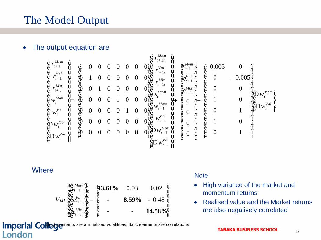
• The output equation are

Where

1|1

1|1

1|1

1 0 0 0 0 0 0 0

0 1 0 0 0 0 0 0

0 0 1 0 0 0 0 0

0 0 0 0 1 0 0 0

0 0 0 0 0 1 0 0

0 0 0 0 0 0 0 0

0 0 0 0 0 0 0 0

Momt tMom

t V alt tVal

t Mktt tMkt

t T ertMom

t

Valt

Momt

V alt

rr

rr

rr

sw

w

w

w

++

++

++

é ù é ùê ú ê úê ú ê úê ú ê úê ú ê úê ú ê úê ú ê úê ú ê úê ú= ê úê ú ê úê ú ê úê ú ê úê ú ê úê úD ê úê ú ê úê ú ë ûDê úë û

1

1

1

1

1

1

1

0.005 0

0 0.005

0 0

1 000 101 000 10

Momt

Valt

Mktm Momt

t

Mom Vt t

Valt

Momt

V alt

w

w w

w

w

w

e

e

e

+

+

+

-

-

-

-

é ùê ú é ùê ú -é ùê úê ú ê úê úê ú ê ú-ê úê ú ê úê úê ú ê úê úê ú ê úê úê ú Dê úê úê ú ê ú+ +ê úê ú ê ú Dê úê ú ê úê úê ú ê úê úê ú ê úê úê ú ê úê úê ú ê úD ê úê ú ê úê úê ú ë ûë ûê úDê úë û

al

é ùê úê úê úë û

1

1

1

0.03 0.02

0.48

Momt

V alt

Mktt

V ar

e

e

e

+

+

+

æ öé ù é ù÷çê ú÷ ê úç ÷çê ú÷ ê úç ÷ê úç = -ê ú÷ç ÷ê ú ê úç ÷÷çê ú ê ú÷ç ÷÷çê ú ê úè ø ë ûë û

13.61%

- 8.59%

- - 14.58%

Note• High variance of the market and

momentum returns• Realised value and the Market returns

are also negatively correlated

Bold Elements are annualised volatilities, Italic elements are correlations

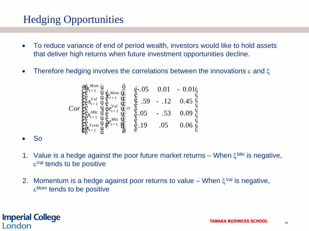
Hedging Opportunities

24

• To reduce variance of end of period wealth, investors would like to hold assets that deliver high returns when future investment opportunities decline.

• Therefore hedging involves the correlations between the innovations ε and ξ

• So

1. Value is a hedge against the poor future market returns – When ξMkt is negative, εVal tends to be positive

2. Momentum is a hedge against poor returns to value – When ξVal is negative, εMom tends to be positive

1

11

11

11

-.05 0.01 0.01

.59 .12 0.45,

.05 .53 0.09

.19 .05 0.06

Momt Mom

tV alt Val

tMktt Mkt

tT ermt

Cor

xe

xe

xe

x

+

++

++

++

æ öé ù é - ù÷çê ú ÷é ùç ê ú÷çê ú ÷ê úç ê ú÷ - -ê úç ê ú÷ ê úç ÷ê ú ê úç ÷= ê ú÷çê ú ê ú -÷ç ê ú÷çê ú ê ú÷ ê úç ÷ê úç ê ú÷ ê úë ûç ÷ê ú ÷ç ë ûè øë û

The Performance Criteria

25

• The cost function is a function of these output variables

• Transaction costs are such that a 10% change in the allocation to value costs 20bp of return and a 5% change costs 5bp of return.

1

1

1

1

10 0 0 0 0 0210 0 0 0 0 02

0 0 0 0 0 0 0

1 0 0 0 0 0 0210 0 0 0 0 02

0 0 0 0 0 0.2 0

0 0 0 0 0 0 0.2

T otalt t t t t

Momt

Valt

Mktt

Momt

Valt

Momt

Valt

r w w T w

r

r

r

w

w

w

w

+

+

+

+

¢ ¢= - D D

¢é ù é ùê ú ê úê ú ê úê ú ê úê ú ê úê ú ê úê ú ê úê ú ê úê ú= ê úê ú ê úê ú ê úê ú ê úê ú ê úê úD -ê úê ú ê úê ú ê ú-Dê ú ê úë ûë û

£

1 1

1 1

1 1

0

0

12

020

0

0

Mom Momt t

Val Valt t

Mkt Mktt t

Mom Momt t

Val Valt t

Mom Momt t

Val Valt t

r r

r r

r r

w w

w w

w w

w w

+ +

+ +

+ +

é ù é ùé ùê ú ê úê úê ú ê úê úê ú ê úê úê ú ê úê úê ú ê ú-ê úê ú ê úê úê ú ê úê úê ú ê ú- ê úê ú ê úê úê ú ê úê úê ú ê úê úê ú ê úê úê ú ê úD Dê úê ú êê úê ú êê úD Dë ûê ú êë û ë û

2t t tz Rz Sz

úúú

¢= -

An Illustration

26

• We shall calculate the optimal portfolio allocations for our earlier example. We shall set θ=20.

• We shall compare our optimal dynamic portfolio to one calculated from the solution to the static problem of finding the optimal portfolio wt given an initial portfolio wt-1 that maximises the Legrangian

where

subject to the weight on the market being equal to 1.

( ) ( )1| 1 1ˆ

2e

t t t t t t t t tL w r w w T w w w wq+ - -

æ ö¢¢ ¢÷ç= - - - - W÷ç ÷çè ø

( ) ( )1|

1| 1|

1|

ˆ and [= 5 : 7, 5 : 7 ]

Momt t

e V alt t t t t

Mktt t

r

r r Var

r

e+

+ +

+

é ùê úê úê ú= W= Wê úê úê úë û

A Comparison of the Static and Dynamic Approaches

27

• We compare for the optimal portfolio weights over our data sample

0.00

0.25

0.50

0.75

1.00

1.25

1.50

1.75

2.00Ja

n-84

Jan-

85

Jan-

86

Jan-

87

Jan-

88

Jan-

89

Jan-

90

Jan-

91

Jan-

92

Jan-

93

Jan-

94

Jan-

95

Jan-

96

Jan-

97

Jan-

98

Jan-

99

Jan-

00

Jan-

01

Jan-

02

Jan-

03

Jan-

04

Jan-

05

W eigh t on M om entum - Stat ic W eigh t on Value - Stat icW eigh t on M om entum - Dynam ic W eigh t on Value - Dynam ic

1. The dynamic solution gives a far greater weight to Momentum

2. The dynamic solution plays value far harder during the value market 1992-1996

Deconstructing the solution - Hedging

28

• Set transactions costs to zero. Differences due to Hedging

1. Dynamic solution increases position on momentum as a hedge against value

2. Dynamic solution increases position on value as a hedge against the market.

-3.00

-2.00

-1.00

0.00

1.00

2.00

3.00

4.00

5.00

Jan-84

Jan-85

Jan-86

Jan-87

Jan-88

Jan-89

Jan-90

Jan-91

Jan-92

Jan-93

Jan-94

Jan-95

Jan-96

Jan-97

Jan-98

Jan-99

Jan-00

Jan-01

Jan-02

Jan-03

Jan-04

Jan-05

Weight on Momentum - Static Weight on Value - StaticWeight on Momentum - Dynamic Weight on Value - Dynamic

Conclusions

29

• We have phrased the dynamic portfolio construction problem in the risk sensitivity framework of Whittle 1991. This framework is very flexible as allows us to model:

• Forecast decay rates

• Forecast uncertainty

• Correlation in forecasts

• Transaction costs – both implicit and explicit

• Portfolio Hedging motives

• We have illustrated the problem on both a long-term strategic asset allocation problem and a shorter term value/momentum trading strategy.

dynamic portfolio optimisationan example of a hedging portfolio 4 • assume returns, r, in any...

Documents