Knorr-Held:

Dynamic Rating of Sports Teams. (REVISED 1999)

Sonderforschungsbereich 386, Paper 98 (1997)

Online unter: http://epub.ub.uni-muenchen.de/

Projektpartner

Dynamic Rating of Sports Teams

Leonhard Knorr�Held

Institut f�ur Statistik

Ludwig�Maximilians�Universit�at M�unchen

Ludwigstr� ��

D����� M�unchen

Germany

Email leo�stat�uni�muenchen�de

First version November ��

Revised March �

Abstract

We consider the problem of dynamically rating sports teams based on the categorical

outcome of paired comparisons such as win� draw and loss in football� Our modelling

framework is the cumulative link model for ordered response� where latent parameters

represent the strength of each team� A dynamic extension of this model is proposed

with close connections to nonparametric smoothing methods� As a consequence� recent

results have more in�uence for estimating current abilities than results in the past� We

highlight the importance of using a speci�c constrained random walk prior for time�

changing abilities which guarantees an equal treatment of all teams� Estimation is done

within an extended Kalman �lter type approach� An additional hyperparameter which

determines the temporal dynamic of the latent team abilities is chosen based on optimal

one�step�ahead predictive power� Alternative estimation methods are also considered�

We apply our method to the results from the German football league �Bundesliga

��� �� and to the results from the American National Basketball Association �NBA�

��� ���

Key words� Constrained Random Walk Prior Cumulative Link Model Dynamic Model

Invariance of Estimators Ordinal Response Paired Comparisons Rating�

�

� Introduction

When sports teams compete in pairs they collect scores or goals within a game� Typically

the winning team the team with more scores at the end of the game gets rewarded with a

certain amount of points while the losing team remains empty�handed� Often there is also

the possibility of a draw where both teams have the same amount of scores and therefore

get rewarded with the same amount of points� For example in football a winning team gets

� points and a draw is rewarded with one point for each team� In general with or without a

draw results from those paired comparisons are essentially given in ordered categories and

mainly those categories determine the standing in the league�

Many approaches for rating sports teams use the score di�erence as the response variable

within standard linear model methodology� Other approaches especially in football use

log�linear Poisson models for the number of goals of both teams� However it is clear that a

rating system should reward a team for winning per se and not for �running up the score�

�Harville ����� This has led many authors to propose robust versions for rating sports

teams based on the score di�erence� For example Harville ���� ���� proposes to truncate

the di�erence at some prede�ned cutpoint whereas Bassett ���� uses L��norm regression�

Taking Harville�s argument to the limit we use only result categories as the basis to rate

teams within a regression model for ordinal categorical data� Thus the main goal here is

rating and not prediction where the score of each team and a lot of other factors should

be considered as possible predictors such as for example the ball control percentage of

each team or the number of spectators� Nevertheless we use the predictive power of our

formulation for model �tting�

Let yij be the result from a paired comparison of team i and team j where team i is the

home team and team j is the visiting team� For example results from football matches are

given in � categories say

yij �

������������ if the home team i wins

� for a draw and

� if the visiting team j wins�

Cumulative link models are a popular framework to analyze paired comparisons� These

models assign a latent ability �i to each team i representing the strength of the team� The

�

model is constructed in a way such that the di�erence in ability of the competing teams

�i � �j a�ects the probabilities of the results yij through a response function F see for

example Agresti �����

An important special case is the cumulative logistic model which boils down to the model

by Bradley and Terry ����� for the case of two possible outcome categories �win loss�� An

extension to more than two categories is discussed in Tutz ������ We give a short review

of the classical non�dynamic cumulative link model in Section ��

When paired comparisons are observed over time it will often be the case that the teams

performances vary over time due to injuries of important players changes of the coach or for

other reasons� Fahrmeir and Tutz ���a� introduce dynamic models for longitudinal paired

comparison data where abilities are allowed to vary smoothly over time� These model can be

seen as Bayesian dynamic models with speci�c smoothing priors and have close connections

to nonparametric smoothing methods since no functional form is speci�ed for the temporal

development of the now time�changing abilities� An extended version of the Kalman �lter

algorithm for categorical data is used to estimate unknown parameters� Similar dynamic

versions of the Bradley�Terry model are proposed independently in Glickman ���� who

uses Markov chain Monte Carlo �MCMC� methods for a full Bayesian analysis�

In Section � we introduce a dynamic model which is based on the approaches above but has

certain amendments� One crucial point is that our model treats all teams symmetrically

which is guaranteed by a speci�c singular multivariate Gaussian distribution as a smooth�

ing prior for the temporal development of the abilities of the teams� Additional thresh�

old parameters which represent a possibly existing home�court advantage are assumed as

time�constant and team�independent� Estimation and prediction is outlined in Section ��

Posterior mode estimators of the abilities are calculated with the extended Kalman �lter

algorithm by Fahrmeir ����� A hyperparameter determining the temporal smoothness of

the abilities of each team can be chosen by maximizing one�step�ahead prediction crite�

ria natural by�products of the extended Kalman �lter algorithm� Such an approach has

a certain optimality feature which is understandable at least in principle to the public�

Alternative ways to estimate the smoothing parameter are an EM�Type algorithm and a

fully Bayesian analysis by MCMC which are also considered� The corresponding software

is available from the author by request�

�

We apply our method to data from the German football league ���� in Section �� A

comparison with estimates by MCMC suggests that inference by the extended Kalman �lter

gives reliable estimates� Furthermore we analyze a larger dataset from the American Na�

tional Basketball Association �NBA� season ����� Here we have found interesting and

pronounced temporal trends in the estimated strength of several teams� Section � concludes

with possible modi�cations and generalizations of our model and some other comments�

� Cumulative Link Model

Let n denote the number of teams in the league and let R denote the number of categories

in the ordinal response scale� A cumulative link model for a comparison yij of a home team

i with a visiting team j is de�ned by

Pr�yij � r� � F ��r � �i � �j�� r � �� � � � � R� �� ���

where F is a distribution function �� � � � � � �R�� are so�called threshold parameters and �i

is the latent ability of team i� For notational convenience we furthermore introduce �� � ��

and �R � �� so that the probability of observing a result yij � r can be written as

Pr�yij � r� � F ��r � �i � �j�� F ��r�� � �i � �j�� r � �� � � � � R�

The threshold parameters are able to represent a home�court advantage an important factor

for nearly all kinds of sports� For illustration consider a match where both teams have the

same ability �i � �j� The probabilities Pr�yij � r� � F ��r� � F ��r��� depend now only

on the thresholds �r and �r��� For example in the case of three categories the larger �� is

the larger is the probability Pr�yij � �� � F ���� that the home team wins� Note that the

home�court advantage is assumed to be the same for all teams�

Estimation of � � ���� � � � � �R���� and � � ���� � � � � �n�

� is done by maximizing the likelihood

the product of individual contributions Pr�yij � r� of all matches� Computation can be done

conveniently with standard software such as SAS PROC LOGISTIC� Note that the model is

unidenti�able because only di�erences of abilities enter in the likelihood� Adding a constant

to �i� i � �� � � � � n� will not change the likelihood� It is therefore necessary to impose an

additional constraint so that the level of the abilities is speci�ed� Usual constraints are

�

nPi��

�i � � or �n � � say� Invariance of the Maximum Likelihood �ML� estimator �e�g� Cox

and Hinkley ���� ensures that estimated abilities are equivalent whatever constraint was

used� For example the ML estimator ���� � � � � ��n�� under the constraint �n � � can be used

to calculate the ML estimator ���� � � � � ��n under the constraintnP

i���i � � by

��i � ��i ��

n

n��Xj��

��j� i � �� � � � � n� �� and ��n � ��

n

n��Xj��

��j� ���

In Section � we will show that this invariance no longer holds for dynamic cumulative link

models�

The estimated abilities �i i � �� � � � � n are the basis for rating teams� This approach has

certain advantages compared to the standard rating based on adding points in football or

counting the number of wins in basketball� In particular because abilities are estimated

simultaneously the approach automatically adjusts for the strength of the corresponding

opponents and for the home�court advantage� Furthermore future games can be predicted�

The ML estimator might not exist for some data constellations due to the discrete nature of

the data� For example a team winning�losing all of its matches will have positive�negative

in�nite estimated ability� It is therefore advisable to check before the analysis that all teams

did not win or lose all of their matches� Singularities will also arise if teams can be partitioned

into two subsets in which none of the teams in one subset competes against any other team

in the other subset� Comparisons within a league however are usually scheduled in a way

that every team competes against any other team in the league so this type of singularity

will not arise�

� Dynamic Cumulative Link Model

��� The basic model

Suppose now that paired comparisons ytij are observed over time t� We consider time t �

�� � � � � T as discrete�valued and equally�spaced such as days weeks or months� Our starting

point is to allow in ��� for time�dependent abilities �ti t � �� � � � � T i � �� � � � � n

Pr�ytij � r� � F ��r � �ti � �tj�� r � �� � � � � R� �� ���

�

This speci�cation allows us to rate sports teams dynamically by estimating time�dependent

abilities� We assume Gaussian �rst order random walks

�ti � N��t���i� ��� ���

as smoothing priors for the abilities of each team i� This is a common assumption for

dynamic modelling of paired comparisons see Glickman ��� �� and Fahrmeir and

Tutz ���a�� The corresponding prior distributions neither impose stationarity nor assume a

speci�c parametric form� in fact model ��� is related to semi� and non�parametric smoothing

methods as reviewed by Fahrmeir and Knorr�Held ���� This paper also indicates how to

generalize the prior to observations which are not made on a regular time grid�

Model ��� implies that recent matches have more weight for estimating current abilities than

results way back into time a natural assumption� The parameter �� determines the weights

and hence the loss of memory rate of the random walks� For the limiting case �� � � the

model reduces to the classical non�dynamic model ����

��� Ensuring exchangeability by a constrained random walk prior

The crucial point is how to impose a smoothing prior on the abilities �t � ��t�� � � � � �tn��

without destroying an exchangeable treatment of the teams� This problem occurs since

as in the time�independent case one has to impose an additional restriction on �t� t �

�� � � � � T to assure identi�ability� It is however not as straightforward as in the time�

independent case because the posterior mode estimator in dynamic models is not invariant

with respect to the identi�ability constraint� We therefore propose a construction based on

a speci�c multivariate singular Gaussian distribution for �t which ensures that marginally

all components of �t follow a �rst order random walk ��� but where the sumnP

i���ti is zero

for each time point t� Harvey ��� pp� ������ has described a related approach where

seasonal dummies sum up to zero�

More formally we assume that �t follows a constrained multivariate Gaussian random walk

�t � �t�� � ut� ut � N��� Q�� t � �� � � � � T� ���

with independent disturbances ut t � �� � � � � T and initial value �� ful�lling ���� � �� Here

� denotes the vector ��� �� � � � � ���� We now specify a speci�c singular dispersion matrix Q

�

of rank n � � which ensures that ��ut � � hence ���t � � for t � �� � � � � T � In general

there are many such matrices Q but � apart from a proportionality constant � there is only

one which treats components of ut exchangeable� A detailed discussion can be found in

Knorr�Held ����� For the case where all components of ut have the same variance �� Q is

given by Q � ���I� �

n����� Here I denotes the identity matrix� The exchangeable treatment

is easily seen because all non�diagonal entries hence all covariances between components

of ut are equal� Furthermore all diagonal entries are equal so marginally and ignoring a

multiplicative factor �n � ���n for the variance every component of �t follows a regular

univariate random walk ���� Note that our model implies that components of ut are a priori

negatively correlated�

It is easily seen that the sum of components of ut is zero because ��ut has variance �

�Q� �

�����I � �

n����� � � and is therefore equal to E���ut� � � with probability one� For the

more general case with individual variances ��i for each team Q is given by Q � L�L� with

L � I � �

n��� and � � diag����� �

��� � � � � �

�n��

It is computationally convenient to consider a linear transformation of ut say Lut where the

�rst n� � components are Gaussian with regular dispersion matrix and the last component

is zero with probability one� For example

L �

�B� I ��

�� �

�CA

is such a transformation matrix� The �rst n � � components of Lut now have dispersion

P � ���I������ One can now perform inference for these n�� a priori positively correlated

components� The transformation M�Lut� with M � I � �

n��� which corresponds to ���

retransforms Lut to ut� The whole approach can also be used in the general case where each

component has its own variance ��i i � �� � � � � n here P � diag����� ��� � � � � � �

�n��� � ��n��

��

Fahrmeir and Tutz ���a� assume independent Gaussian �rst order random walk priors for

all but one team say

�ti � �t���i � uti� uti � N��� ��i �� i � �� � � � � n� �� t � �� � � � T� ���

and �x the ability of the last team to zero for each time point t� They also use a similar

strategy for other smoothing priors such as the local linear trend model� After estimation

�

they recenter the estimates to mean zero for every time point t using the transformation

matrix M from above� However this approach does not treat teams symmetrically because

of the prior independence of the random walks a change of the reference team will lead

to di�erent ratings� This can be best seen for the case where all random walks have the

same variance �� The recentered increments uti� i � �� � � � � n� � now have variance �����

��n��n����n�� while increments of the reference team have variance ���n����n� which is

much smaller� The estimated abilities of the reference team will show less temporal variation

then all the others� For example for n � �� as in the football example in Subsection ���

the standard deviation of the recentered uti is ����� i � �� � � � � n � � while the standard

deviation of utn is ������� This di�erence increases as n increases� Note that in the more

general case with team�speci�c variances ��i the variance ��n of team n does not even occur

in the model speci�cation ��� and can therefore not be estimated from the data�

Model ��� can easily be modi�ed to achieve a symmetric treatment of the teams� Replace�

ment of the independent random walk priors for the n � � components with the correlated

multivariate random walk with covariance matrix P will give a model which is equivalent to

the constrained random walk model ��� as outlined above�

Recently Glickman and Stern ���� �short GS� use a related but slightly di�erent approach

for �xing the overall level of the time�dependent abilities� They propose that not �t but the

mean of �tj�t��� �� is centered at zero

�tj�t��� �� � N�M�t��� �

�I� ���

with M as de�ned above� Thus the sum of components of �t ���t has expectation zero and

variance n�� whereas in our model ���t has both expectation and variance equal to zero�

There is an important di�erence between the GS and our approach� Both are equally valid

to predict future game outcomes as only di�erences of team abilities enter in the likelihood

implied by ���� Also for a given time t teams can be ranked or rated based on the GS

estimates as well as on our estimates� However the GS model is not readily usable for

judging the temporal development of a given team� For example suppose team i has no

match scheduled at time t� We would then expect the team�s ability to be the same as in

time t � � no matter what the abilities of the other teams are at time t � � and this is

exactly what out formulation implies� However in the GS model the expected ability of this

�

team is �ti � �t���i ��

n

nPj��

�t���j� Hence the expected ability might raise or drop although

the team has not performed any game at all� Strictly speaking estimated abilities in the GS

model can only be interpreted for a given time t but not for a given team i� Our model has

the advantage that here estimated abilities are valid quantities to assess the performance

of a speci�c team over time� Note that the primary focus in Glickman and Stern ���� is

prediction and for this model ��� is equally well suited�

� Estimation and prediction

��� The extended Kalman �lter and smoother

For the moment consider �� as �xed� We use the extended Kalman �lter and smoother

�EKF� by Fahrmeir ���� and Fahrmeir and Tutz ���a� to estimate time�dependent

abilities� A detailed description can be found in Fahrmeir and Tutz ���b� Chapter ��

Threshold parameters � are estimated by Maximum Likelihood given the current �smoothed�

estimates of �� Both steps �EKF�estimation of � for �xed � and ML�estimation of � for �xed

�� are alternated until convergence which takes only a few seconds on a standard workstation

or a Pentium PC in both of our applications�

The EKF algorithm starts with an initial value �� a pre�season estimate of the abilities

and then subsequently estimates �t t � �� � � � � T on the basis of all games played until

time t� This is called the �ltering step and gives �ltered estimates ��t� In a second step

the smoothing step �ltered estimates ��t t � T � �� � � � � � are smoothed on the basis of all

games played until time T � The smoothed estimate of �� is used as a new initial value in the

next iteration� The algorithm requires an initial value for the prior dispersion Q� say of ���

In our applications we used Q� � I� �

n��� which is weakly informative but avoids numerical

problems with more di�use priors� The �nal estimates of �� are virtually identical whatever

starting value for �� was used�

This algorithm can be derived as an approximate posterior mode estimator e�g� Fahrmeir

and Tutz ���b�� Alternatively one could use iterative EKF �Fahrmeir and Wagenpfeil

��� which gives the exact posterior mode� Computation time increases however because

an additional level of iteration is required� Furthermore di�erences between estimates by

non�iterative and iterative EKF are typically small� See the references above for more details

on properties of posterior mode estimators�

The estimates of �T and � can be used to predict future matches� For example suppose

team j is scheduled to visit team i are next round �t � T � �� to perform a match� The

probabilities of the outcomes Pr�yT���ij � r� r � �� � � � � R can be estimated by model ���

Pr�yT���ij � r� � F ���r � ��T i � ��Tj�� F ���r�� � ��T i � ��Tj�� ���

because the �rst order random walk assumption for �t gives ��T as the predicted ability at

time T � �� Note that �ltered and smoothed estimates of �T coincide� More general one�

step�ahead predictions are used later to assess the prediction quality and to estimate the

smoothing parameter ���

��� Estimating the smoothing parameter by maximizing the pre�

dictive power

In the following we propose to estimate the smoothing parameter �� based on one�step�

ahead prediction� Alternative ways are outlined afterwards�

Above it was sketched how �ltered estimates ��T can be used to predict future games� Filtered

estimates ��t are also available for t � �� � � � � T � � from the extended Kalman �lter so we

are able to perform a retrospective one�step�ahead prediction to assess the model �t� This

is done by subsequently predicting outcomes at time t�� based on �ltered estimates ��t and

comparing the predicted probabilities with the actual observed result by some criterion�

Let N be the total number of paired comparisons over the whole time period� We suppress

dependence on time t and opponents i and j and denote the predicted probabilities Pr�yk �

s� of outcomes s � �� � � � � R by �pk�s� k � �� � � � � N � These predictions are calculated based

on �ltered estimates ��t similar to ��� given only game information prior to period t � ��

A comparison of the actual observed result yk � r with the predicted probabilities can be

done by various criteria� We have implemented the following four concordancy measures

C� �NXk��

�

�argmaxs�������R

�pk�s� � r

�

��

C� ��

N

NXk��

log �pk�r��

C� � ��

N

NXk��

�f�� �pk�r�g� �X

s ��r

f�pk�s�g�

� and

C� ��

N

NXk��

�pk�r��

Criterion C� is the number of correctly predicted games where those outcomes are predicted

which have the highest predictive probability� Criterion C� is a log�likelihood criterion and

is used also by Glickman ��� in a similar approach to select hyperparameters� Measure

C� is based on quadratic loss while C� is equivalent to the corresponding measure based on

absolute loss� Similar criteria are used in discriminant analysis and nonparametric regression

for estimating smoothing parameters by cross�validation see for example Fahrmeir and Tutz

���b� p� ���� We perform a separate estimation of � and � as outlined in Section ���

for each of a large number of values of �� between zero and one� The smoothing parameter

�� will then be chosen on the basis of maximal predictive concordancy with respect to the

corresponding criterion�

When T is small it is often the case that some or all of the criteria are maximized for the

limiting case �� � �� For larger T there will often be evidence for time�changing abilities

and �at least some of� the criteria are maximized for truly positive values of ��� Note that

the �zero�one� criterion C� has the a bit unattractive feature that it is not continuous as a

function of �� so that optimal values of the smoothing parameter �� are typically within a

certain interval� All other criteria are continuous functions of ���

��� Alternative estimation methods

Alternatively an EM�type algorithm can be implemented to estimate �� see for example

Harvey ���� or Fahrmeir and Tutz ���b�� A disadvantage of this method is rather slow

convergence� We have nevertheless implemented an EM�type algorithm for �� and report

the corresponding estimates in our applications for comparison with the estimates based on

predictive concordancy�

��

For a fully Bayesian analysis MCMC methods can be used to make simultaneous inference

about all unknown parameters� Such methods require speci�cation of a prior distribution

for the threshold parameters � and the variance ��� While for the former improper priors

�uniform on the whole real line� can be chosen for the latter proper priors have to be used as

to avoid problems with improper posteriors� Computationally convenient are inverse gamma

priors say �� � IG�a� b� with �xed values of a and b� Typical �weakly informative� choices

are a � � and b small say ����� ���� or ��� �e�g� Besag Green Higdon and Mengersen

����

An advantage of MCMC is that the uncertainty about the estimated parameters � and ��

is incorporated in the estimation of � and that samples from predictive distributions can

be generated� Note however that standard MCMC methods do not give �ltered estimates

an issue that will be further discussed in Section �� We have also implemented an analysis

of dynamic paired comparison models by MCMC to assess the accuracy of our algorithm�

Updating of components of � was done by Gaussian Metropolis proposals �e�g� Smith

Roberts ��� while updating of abilities was done by �multivariate� conditional prior

proposals �Knorr�Held �� for each vector �t� Note that for inference by MCMC the

initial value �� can be omitted in the model formulation�

� Applications

In the following we illustrate our method with two applications� We use the dynamic cumu�

lative link model ��� with the logistic response function F �x� � ��f� � exp��x�g together

with the constrained random walk prior ���� We have also tried the extreme�minimal�value

distribution function F �x� � �� expf� exp�x�g which however did not �t the data as well

as the logistic model in terms of predictability� We do not display �approximate� point�

wise credible intervals which are available from the extended Kalman �lter for reasons of

presentation�

��

��� The German football league ���

In the ���� season of the German football league �Bundesliga� n � �� teams compete

for the German championship� Teams meet each other twice within the season giving each

team the home�court advantage once� In total N � ��� matches were performed between

August ��th �� and May ��th ��� We have categorized the time scale in T � ��

calendar weeks which gives roughly one match per team and per time point� Note that there

is a winter break between December �th �� and February ��th �� where no matches

took place� As noted in the introduction possible outcomes are given in R � � categories

win �y � �� draw �y � �� and loss �y � �� of the home team� Based on these results points

are assigned to the teams �� for a win � for a draw� which determine the standings in the

league table� Table � gives the �nal standings of the ���� season�

We have estimated the smoothing parameter �� based on all four prediction criteria� Crite�

rion C� the absolute loss criterion and criterion C� agree very much in �tting the optimal

model C� is maximized for �� � ������ with a value of ������ compared to ����� for

�� � �� Criterion C� is maximized around �� � ���� with ��� correctly predicted games

���� for �� � ��� The EM�type estimate is slightly lower with ��� � ������� Convergence

was very slow� This indicates that there is not much information on temporal variation of

abilities in the data� In fact the other two criteria C� and C� are maximized for the limiting

case �� � �� The reason might be that they both give relatively more weight to small values

of �p�k� than C� and C�� Small estimated probabilities are more likely for large values of ��

where estimated abilities have more temporal variation and cause estimated probabilities to

be more extreme�

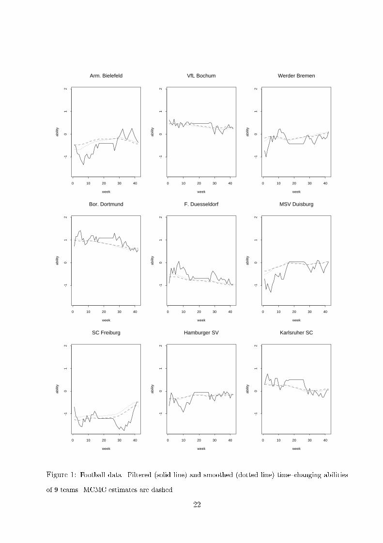
Figures � and � show �ltered and smoothed estimated abilities of all �� teams for �� �

������� The smoothed estimates show rather di�erent patterns for the di�erent teams and

demonstrate the advantages of our nonparametric dynamic model� Note also that within the

winter break �t � ��� � � � � ��� �ltered estimates are horizontal lines due to the prior model�

Later champion Bayern M�unchen has a rather time�constant performance with smoothed

abilities between ��� and ���� Other teams however have a substantial time�dependent

performance� For example Borussia M�onchengladbach has a rather poor performance before

the winter break while its estimated ability at the end of the season was even slightly above

��

average with a value of ����� Interestingly this change of performance coincidences with the

dismissal of the head coach shortly before Christmas� SC Freiburg shows a similar dynamic

but in contrast to M�gladbach the better performance towards the end of the season did

not pay out The team had to be relegated from �rst to second division�

Estimates of threshold parameters are �� � ������� ����� and re!ect a strong home�court

advantage already apparent in the raw data ����" of all matches were won by the home

team and only ����" by the visiting team�

For comparison we have analyzed this dataset also by MCMC� Table � gives posterior mean

estimates of �� and � for a � ��� and various values of b� There is a strong sensitivity of the

results especially of ��� with respect to the prior for ��� Consequently the estimated abilities

di�er very much with the degree of smoothness determined by ���� Unfortunately there are

no clear guidelines how to choose the prior for ��� For a � � and b � ��� which comes

closest to the C��estimate ��� � ������ we have calculated posterior mean estimates of the

ability parameters which are also displayed in Figures � and �� From these pictures it can

be seen that the MCMC estimates are rather similar to the smoothed estimates from the

extended Kalman �lter� Hence the Kalman �lter algorithm gives quite reliable results here�

The small di�erences which seem to depend on the absolute value of ��it may be caused

by the approximateness of the EKF algorithm the slightly di�erent model formulation for

MCMC with all parameters stochastic and without �� or by skewed posterior distributions

where posterior means and modes do not coincide� In a second MCMC analysis we have

�xed �� � ����� and the small di�erences between means and modes have slightly decreased�

��� Season ��� of the National Basketball Association

In the American National Basketball Association �NBA� n � � teams have performed

paired comparisons in the ���� season� We analyze N � ��� games excluding results

from the play�o�s� These games took place between November �st �� and April ��th

�� which gives a total of T � ��� calendar days� Note that in Basketball there is not

the possibility of a draw because of the overtime rule� Games can only end with R � �

categories�

Our model �t criteria show a similar behaviour as for the football data C� and C� again

��

agree very much� Criterion C� is optimal around �� � ����� with ��� correctly predicted

games ���� for �� � ��� C� has an optimal value of ������ for �� � ������ compared

to ������ for �� � �� The EM�Type estimate is also rather close with ��� � �������� The

log�likelihood criterion C� and the quadratic loss function criterion C� however again prefer

the non�dynamic model ��� � ��

The following results are based on the C��optimal value �� � ������� The threshold

parameter was estimated by �� � ���� re!ecting a substantial home�court advantage� Filtered

and smoothed estimated abilities of selected teams are shown in Figure �� Interestingly the

Chicago Bulls the later champion have a steadily declining performance� They might have

not played with full force towards the end of the season being already quali�ed for the

play�o�s� Other teams such as the Houston Rockets the Phoenix Suns or Utah Jazz have a

very remarkable dynamic which would have been overlooked by a parametric model where

for example abilities are assumed to develop linear or quadratic in time�

� Concluding Remarks

This paper discusses the application of dynamic cumulative link models for rating sports

teams� Our prior model ensures a symmetric treatment of all teams assuming a multivariate

singular Gaussian random walk prior with exchangeable components� Similar priors can also

be used if the response variable is the di�erence in score between the home and the visiting

team which is the more traditional approach to rating and prediction because estimation can

be done within the standard linear model see for example Harville ���� ���� or Harville

and Smith ����� A dynamic approach for modelling the score di�erence within the state�

space model is proposed in Sallas and Harville ������ There are also areas outside of dynamic

models for paired comparisons where constrained random walk priors are potentially useful�

For example dynamic modelling of categorical covariate e�ects with constrained random

walk priors is used in Knorr�Held and Besag ���� for space�time modelling of disease risk

data�

Estimation of the smoothing parameter turned to be di#cult� The reason seems to be that

the type of categorical data does not provide much information about the temporal variation

��

of teams abilities� Among the four di�erent measures both the �zero�one� and the absolute

loss function criterion showed a good performance whereas the other two choices have been

disappointing� As an alternative an EM�Type algorithm can be used which however has

rather poor convergence properties� Fully Bayesian estimation by MCMC was very sensitive

with respect to hyperprior speci�cations�

A referee has suggested to consider �independent� stationary autoregressive processes as a

prior model for the abilities of each team i � �� � � � � n

�ti � N�i � ��t���i � i�� �

��

��i � N

�i�

��

�� �

�

The parameter i could be interpreted as the long term average ability of team i� Such a

model has the advantage that a priori the abilities of the teams will in the long run not

tend towards � or � in�nity� Estimation can be done by MCMC� Also identi�ability can

easily be achieved by �xing the mean ability of a particular team say the nth to zero

i�e� n � � and it does not matter here which teams mean performance is �xed� However

such a model is less parsimonious and therefore problems of sensitivity with respect to now

two hyperparameters �� and are likely to increase� For data over a rather short time

period like in both of our applications it seems that our approach will be !exible enough

and long run behaviour properties of the prior model are not as crucial from an applied point

of view�

There are several possible generalizations of our model� As already noted in Section � each

team can have assigned a team�speci�c smoothing parameter ��i � This might be appropriate

if there is substantially more data than in both of our applications where information about

the temporal variation summarized in �� seemed to be rather small� Furthermore it will

be very di#cult for moderate to large size of n to �nd the optimal values of ��� � � � � � ��n based

on one�step�ahead prediction� Similar comments apply to more enhanced smoothing priors

such as the second order random walk where independent �rst di�erences ��t � �t���� are

replaced by second di�erences ��t� ��t�� � �t���� or the local linear trend model �Harvey

���� Based on our experience with these priors we believe that they have limited use as

long as rating of sports teams within one season is considered as in our two applications�

They might be useful if considerable more data is observed over a longer period�

��

Throughout this paper we have used constant threshold parameters� This assumption can

be relaxed allowing for team�speci�c or time�dependent threshold parameters� Harville

and Smith ���� analyze college basketball results with various models and �nd team�

to�team di�erences in the home�court advantage to be relatively small� Knorr�Held ����

analyzes the German football Bundesliga ����� season� by MCMC with additional team�

speci�c random e�ects for the thresholds but there was not much evidence for a home�court

advantage heterogeneity here either� Fahrmeir and Tutz ���a� allow for time�dependent

threshold parameters in an analysis of the German Bundesliga but �nd threshold estimates

to be stable even over a period of �� years� We have therefore used the simple model with

constant threshold parameters� If necessary it would be no problem to extend our approach

to more general models�

For the application considered we prefer the extended Kalman �lter for statistical inference

rather than MCMC methods� Although MCMC is a more elaborate approach it seems

to be much easier to obtain �ltered estimates by the extended Kalman �lter� These �ltered

estimates can be used to assess the predictive power and to choose the smoothing parameter�

Furthermore in a full Bayesian analysis there seems to be often strong sensitivity with

respect to hyperprior speci�cations� However recently several interesting proposals have

been made to obtain �ltered estimates by dynamic MCMC methods e�g� Gordon Salmond

and Smith ���� Berzuini Best Gilks and Larizza ���� and Pitt and Shephard ����

Application of these approaches to dynamic ordered paired comparison systems are due to

the high dimensionality of the model beyond the scope of this paper�

References

Agresti� A� ������ Analysis of ordinal paired comparison data� Applied Statistics ��� ��������

Bassett� G� W� J� ������ Robust sports ratings based on least absolute errors� The American

Statistician ��� ������

Berzuini� C�� Best� N� G�� Gilks� W� R� and Larizza� C� ������ Dynamic conditional inde�

pendence models and Markov chain Monte Carlo methods� Journal of the American Statistical

Association ��� �������

��

Besag� J� E�� Green� P� J�� Higdon� D� and Mengersen� K� ������ Bayesian computation

and stochastic systems �with discussion�� Statistical Science ��� �����

Bradley� R� A� and Terry� M� E� ������ Rank analysis of incomplete block designs I� The

method of pair comparisons� Biometrika ��� ��������

Cox� D� R� and Hinkley� D� V� ������ Theoretical Statistics� London� Chapman and Hall�

Fahrmeir� L� ������ Posterior mode estimation by extended Kalman �ltering for multivariate

dynamic generalized linear models� Journal of the American Statistical Association � ���

����

Fahrmeir� L� and Knorr�Held� L� ������ Dynamic and semiparametric models� inM� Schimek

�ed��� Smoothing and Regression� Approaches� Computation and Application� New York� John

Wiley � Sons� To appear�

Fahrmeir� L� and Tutz� G� ����a�� Dynamic stochastic models for time�dependent ordered

paired comparison systems� Journal of the American Statistical Association �� ��������

Fahrmeir� L� and Tutz� G� ����b�� Multivariate Statistical Modelling Based on Generalized

Linear Models� New York� Springer�Verlag�

Fahrmeir� L� and Wagenpfeil� S� ������ Penalized likelihood estimation and iterative Kalman

smoothing for non�Gaussian dynamic regression models� Computational Statistics � Data

Analysis ��� ��������

Glickman� M� E� ������ Paired Comparison Models with Time�Varying Parameters� Ph�d�

dissertation� Department of Statistics� Harvard University�

Glickman� M� E� ������ Parameter estimation in large dynamic paired comparison experiments�

Applied Statistics� forthcoming�

Glickman� M� E� and Stern� H� S� ������ A state�space model for National Football League

scores� Journal of the American Statistical Association ��� ������

Gordon� N� J�� Salmond� D� J� and Smith� A� F� M� ������ A novel approach to non�linear

and non�Gaussian Bayesian state estimation� IEE�Proceedings F ���� ������

Harvey� A� C� ������ Forecasting� Structural Time Series Models and the Kalman Filter� Cam�

bridge� University Press�

Harville� D� A� ������ The use of linear�model methodology to rate high school or college

football teams� Journal of the American Statistical Association �� ��������

��

Harville� D� A� ������ Predictions for National Football League games via linear�model method�

ology� Journal of the American Statistical Association �� �������

Harville� D� A� and Smith� M� H� ������ The home�court advantage� How large is it� and

does it vary from team to team�� The American Statistician �� ������

Knorr�Held� L� ������ Hierarchical Modelling of Discrete Longitudinal Data� Applications of

Markov Chain Monte Carlo� M�unchen� Herbert Utz Verlag Wissenschaft�

Knorr�Held� L� ������ Conditional prior proposals in dynamic models� Scandinavian Journal

of Statistics ��� ������

Knorr�Held� L� and Besag� J� ������ Modelling risk from a disease in time and space� Statistics

in Medicine �� ����������

Pitt� M� K� and Shephard� N� ������ Filtering via simulation� auxiliary particle �lters� Journal

of the American Statistical Association� forthcoming�

Sallas� W� M� and Harville� D� A� ������ Noninformative priors and restricted maximum

likelihood estimation in the Kalman �lter� in J� C� Spall �ed��� Bayesian Analysis of Times

Series and Dynamic Models� New York� Marcel Dekker� pp� ��������

Smith� A� F� M� and Roberts� G� O� ������ Bayesian computation via the Gibbs sampler and

related Markov chain Monte Carlo methods �with discussion�� Journal of the Royal Statistical

Society B ��� �����

Tutz� G� ������ Bradley�Terry�Luce models with an ordered response� Journal of Mathematical

Psychology ��� �������

Acknowledgements

The author expresses thanks to Ludwig Fahrmeir an associate editor and to two referees

for several suggestions which have improved the paper�

�

Rank Team Points at home away

� B� M�unchen �� �� ��

� Bay� Leverkusen � �� ��

� Bor� Dortmund �� �� ��

� VfB Stuttgart �� �� ��

� VfL Bochum �� �� ��

� Karlsruhe SC � � ��

� ���� M�unchen � �� �

� Werder Bremen �� �� ��

MSV Duisburg �� �� ��

�� �� FC K�oln �� �� ��

�� M�gladbach �� �� ��

�� Schalke �� �� �� ��

�� Hamburger SV �� �� ��

�� Arm� Bielefeld �� �� ��

�� Hansa Rostock �� �� ��

�� F� D�usseldorf �� �� ��

�� SC Freiburg � �� �

�� St� Pauli �� � �

Table � Final ranking for the ���� season�

��

a b ��� ��� ���

� ���� ������ ����� ����

� ��� ����� ����� ����

� ��� ������ ����� ����

� � ������ ����� ����

Table � Parameter estimates �posterior means� by MCMC for various hyperprior speci�cations�

��

week

abili

ty

0 10 20 30 40

-10

12

Arm. Bielefeld

week

abili

ty

0 10 20 30 40

-10

12

VfL Bochum

week

abili

ty

0 10 20 30 40

-10

12

Werder Bremen

week

abili

ty

0 10 20 30 40

-10

12

Bor. Dortmund

week

abili

ty

0 10 20 30 40

-10

12

F. Duesseldorf

week

abili

ty

0 10 20 30 40

-10

12

MSV Duisburg

week

abili

ty

0 10 20 30 40

-10

12

SC Freiburg

week

abili

ty

0 10 20 30 40

-10

12

Hamburger SV

week

abili

ty

0 10 20 30 40

-10

12

Karlsruher SC

Figure � Football data� Filtered �solid line� and smoothed �dotted line� time�changing abilities

of � teams� MCMC estimates are dashed�

��

week

abili

ty

0 10 20 30 40

-10

12

1. FC Koeln

week

abili

ty

0 10 20 30 40

-10

12

Bay. Leverkusen

week

abili

ty

0 10 20 30 40

-10

12

M’gladbach

week

abili

ty

0 10 20 30 40

-10

12

B. Muenchen

week

abili

ty

0 10 20 30 40

-10

12

1860 Muenchen

week

abili

ty

0 10 20 30 40

-10

12

St. Pauli

week

abili

ty

0 10 20 30 40

-10

12

Hansa Rostock

week

abili

ty

0 10 20 30 40

-10

12

Schalke 04

week

abili

ty

0 10 20 30 40

-10

12

VfB Stuttgart

Figure � Football data� Filtered �solid line� and smoothed �dotted line� time�changing abilities

of the other � teams� MCMC estimates are dashed�

��

day

abili

ty

0 50 100 150

-2-1

01

23

Chicago Bulls

day

abili

ty

0 50 100 150

-2-1

01

23

Houston Rockets

day

abili

ty

0 50 100 150

-2-1

01

23

Miami Heat

day

abili

ty

0 50 100 150

-2-1

01

23

New York Knicks

day

abili

ty

0 50 100 150

-2-1

01

23

Orlando Magic

day

abili

ty

0 50 100 150

-2-1

01

23

Phoenix Suns

day

abili

ty

0 50 100 150

-2-1

01

23

Seattle Supersonics

day

abili

ty

0 50 100 150

-2-1

01

23

Utah Jazz

day

abili

ty

0 50 100 150

-2-1

01

23

Vancouver Grizzlies

Figure � Basketball data� Filtered �solid line� and smoothed �dotted line� time�changing abilities

of selected teams�

��