1

Dynamic Testing of Free Field Response in

Stratified Granular Deposits

L. Dihoru*, S. Bhattacharya**, F. Moccia***, A.L. Simonelli***, C.A. Taylor*, G. Mylonakis*

* University of Bristol, University Walk, Bristol, BS8 1TR, United Kingdom

**University of Surrey, Guildford, GU2 7XH, United Kingdom

***University of Sannio, Piazza Roma 21, Benevento, 82100 Italy

ABSTRACT

The dynamic free field response of two stratified deposits with different stiffness ratios between

the top and the bottom layer was analysed by shaking table testing. The granular deposits were

contained in a laminar shear box and subjected to a wide set of dynamic inputs with different

frequency content. Two exploratory modal testing techniques were employed to measure the

natural frequency of the individual layers and the results were employed in the calculation of the

fundamental period of the overall stratified profile by an extended variant of the Madera procedure

[1]. The dynamic response was investigated in relation to the frequency content of the dynamic

excitation, the granular material properties and the stiffness characteristics of the enclosing

container. The measured dynamic stiffness for the mono-layered and the bi-layered sand deposits

compare well with previous empirical curves for sands increasing the confidence in the shaking

table and shear stack testing as tools of dynamic investigation of granular media.

Keywords: layered soil, 1-g testing, laminar shear box, shaking table

1. Introduction

The shearing stress-strain behaviour of soils is key to understanding how sites and buildings

respond to earthquakes. The effect of local soil conditions on the observed magnitude and patterns

of seismic damage to buildings has been studied extensively in the last four decades [2-7]. The

shearing behaviour of soils, notably the shear modulus and damping ratio were found to be the

properties that govern dynamic soil-structure interaction at all strain levels. The measurement of

these properties has been the central objective in numerous laboratory and field studies [8-13].

Among the various tools employed in the dynamic analysis of granular media, shaking table testing

is an important one, due to its capability of reproducing a wide set of real and artificial seismic

inputs with relevance for the free field response. A large number of shaking table studies [14-18]

employ flexible container boxes (‘shear stacks’) designed to replicate the free field response of a

soil in plane strain conditions. Their role is to shear the soil via vertically propagating shear waves

produced by the accelerating shaking table. In a large scale shear stack a large volume of soil can

be tested, therefore the results may be more representative of the prototype field conditions. The

boundary effects in a large shear stack are smaller than in table-top shear devices and the volume

of soil situated in the central part of the container reproduces better the free field conditions for a

given wavelength. It is also known that the design of a shear stack can be tuned to operate over

wide strain ranges with granular materials of different stiffness value [19]. This, in particular,

makes the shear stack useful for studying the large-strain dynamic moduli under seismic excitation.

Several laminar shear box designs have been reported for both uniaxial and biaxial loading [20-

26]. While there is a large body of literature on tests on homogeneous soils, experimental data on

stratified deposits is scarce. This paper presents an experimental programme of dynamic testing

Corresponding author: L. Dihoru, Dept. of Civil Engineering, University of Bristol, University Walk,

BS8 1TR, Email: Luiza.Dihoru@bristol.ac.uk, Tel. +44-117-3315714

2

carried out on three deposits of dry granular material at Bristol University. An homogeneous

deposit of sand and two bi-layered deposits of sand and rubber granules were tested in a uniaxial

shear stack. The shear stack was assembled rigidly on the platform of a shaking table. Pulse tests

and random white noise tests were carried out to measure the natural frequency of the individual

layers. The fundamental periods of the stratified deposits were evaluated and compared to an

analytical solution from the literature ([1]). The influences brought by the particulate material

characteristics and the dynamic input parameters on the free field response were analysed. Aspects

such as container-deposit coupling and deposit mode shapes were interpreted in relation to the

deposit stiffness and the applied dynamic inputs.

2. Experimental Programme

2.1 Shear Stack

The shear stack employed in this study was a medium-sized uniaxial laminar container of length

1.2 m, width 0.5 m and height 0.8 m. The shear stack was built at Bristol University in 1993 [20]

and has been since subjected to several design improvements directed in particular towards

lowering its stiffness [27]. Previous investigations of the shear stack have shown that its

fundamental frequency when empty is about 6 Hz. The stack is active in one direction only, with

its eight aluminium rings designed to move freely in the direction of shaking. The response in the

other two directions is blocked by a steel rigid frame and a system of bearings. The stack end walls

and base have a rough surface to allow complementary shear stresses to develop. Its side walls are

lubricated to allow uniform plane strain conditions in the deposit. The shear stack is installed on

the platform of a six-degrees-of-freedom earthquake simulator (the ‘shaking table’). The shaking

table consists of a 3 m x 3 m cast aluminium platform weighing 3.8 tonnes and is capable of

carrying a maximum payload of 15 tonnes. A wide set of dynamic inputs such as sinusoidal waves,

sinusoidal sweep waves, real or artificial earthquakes can be reproduced, making the shaking table

a versatile tool for dynamic testing. Horizontal accelerations of up to 3.7 g (with no payload) and

up to 1.6 g (with 12 tonnes payload) can be achieved.

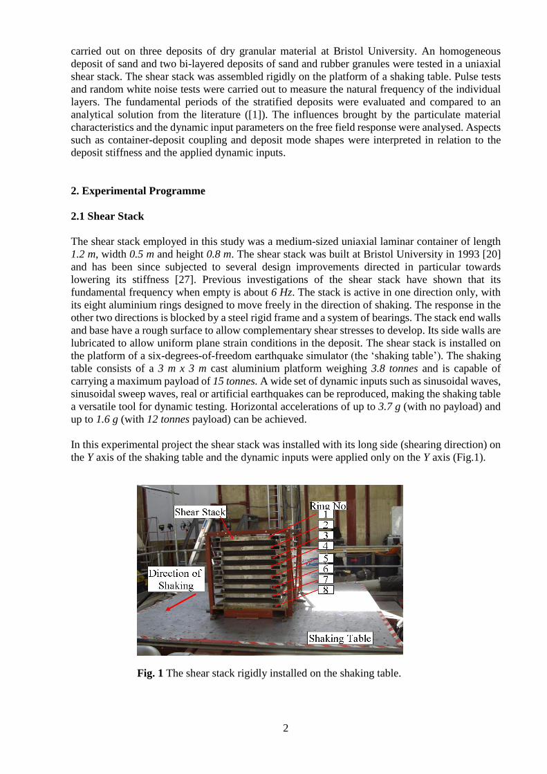
In this experimental project the shear stack was installed with its long side (shearing direction) on

the Y axis of the shaking table and the dynamic inputs were applied only on the Y axis (Fig.1).

Fig. 1 The shear stack rigidly installed on the shaking table.

3

2.2 Materials and Experimental Set-Up

The programme of testing employed three granular materials with different particle properties:

Leighton Buzzard (LB) sand BS 881-131, Fraction B and Fraction E (Table 1) and rubber granules

type Charles Lawrence CT0515B.

Table 1 Leighton-Buzzard sand BS 881-131 Fraction B and Fraction E particle size distribution BS 1881-131 Fraction B BS 1881-131 Fraction E

1180 µm 10% maximum retained 150 µm 15% maximum retained

600 µm 10% maximum passing

90 µm 15% maximum passing

80% minimum between 1180 µm and 600 µm

70% minimum between 150 µm and 90 µm

One monolayer configuration (E) and two layered configurations (BEE and ER) were built by

pluviation. For the layered configurations, the median line of the enclosing container (z =0.4 m)

marked the interface between the two layers of contrasting stiffness. The layout and the stiffness

ratio between the top and the bottom layers for the selected configurations are shown in Fig. 2. A

mixture of LB-Fraction B and LB-Fraction E particles was employed to model the stiff bottom

layer in the BEE configuration. The mean diameter ratio between the two fractions of sands (D50-

Fraction B : D50-Fraction E = 5.77) was considered beneficial for an increase of packing when the two

types of particles were mixed together. The fine particles were expected to fill in efficiently the

voids in the large particle matrix. The mass composition (denoted by X) corresponding to the

theoretical maximum packing density of the mixture was calculated according to a classic model

of packing [28], resulting in XFraction B: XFraction E = 85:15.

Fig.2 Deposit configurations employed in testing (E: monolayered, BEE and ER: two layered).

Further densification of the bottom layer after pluviation was achieved by tapping the deposit on

a shaking table. After 10000 cycles of vertical sinusoidal vibrations of 10 Hz frequency and 0.35

g amplitude, a 5% density gain was achieved (from 1840 kg/m3 to 1942 kg/m3) The upper

prototype layer of lower stiffness was modelled with either Leighton Buzzard Fraction E (in the

BEE configuration) or rubber granules CT0515 (in the ER configuration), respectively. The

material properties, the parameters employed in pluviation and the experimentally obtained bulk

densities are presented in Table 2. A uniform densification was achieved throughout the depth of

the individual deposits.

Table 2 Material properties

Rubber

Particles

CT0515

Sand

LB

Fraction E

Sand

Mixture

LB Fraction B and Fraction E

(85:15)

Mean Diameter, D50 (mm) 1 0.142 0.82

Particle Morphology irregular angular angular

Particle Texture rough smooth smooth

Specific Gravity (g / cm3) 1.15 2.65 2.65

Poisson’s Ratio 0.49 0.31 0.31

Pluviation Parameters:

Nozzle Diameter (mm) / Height of Fall

(mm)

15 / 1000

40 / 1000

15 / 1000

Pluviated Density (kg / m3) 479 1400 1942

LB-Fraction E

LB-Fraction E

LB-Fraction E +

LB-Fraction B

Rubber CT0515

LB-Fraction E

E BEE ER

Gbottom / Gtop= 1.75 Gbottom / Gtop= 80

H=0.8 m

H/2=0.4 m

H/2=0.4 m

LB-Fraction E

LB-Fraction E

LB-Fraction E +

LB-Fraction B

Rubber CT0515

LB-Fraction E

E BEE ER

Gbottom / Gtop= 1.75 Gbottom / Gtop= 80

H=0.8 m

H/2=0.4 m

H/2=0.4 m

Y

Z

4

Four free-field accelerometers (a1-5) were embedded inside the deposit at similar coordinates in

the horizontal plane (x, y) = (0.270, 0.455) m and at vertical intervals of Δz = 0.2 m one from

another. The response of the shear stack was measured by four accelerometers (a6-9) attached to

the outside of the box rings (Fig. 3).

Fig. 3 Accelerometer layout in the shear stack (top: elevation, bottom: plan view,

‘a’: accelerometer position)

2.3 Exploratory Modal Testing

The low strain stiffness of the deposits was measured by modal testing involving sinusoidal pulses

and random white noise. Pulse testing employed half-sinusoidal pulses of 10 Hz frequency,

generated by the shaking table in the Y direction. The measured travel time of the shear wave

between accelerometers served for computing the shear wave velocity. The second modal testing

technique employed a random white noise signal of 1-100 Hz bandwidth and RMS=50 mV (‘Root

Mean Squared’ voltage) generated by the shaking table in the Y direction. Frequency response

functions (FRFs) were calculated by normalising the output of the receiving accelerometer (a2-5 in

Fig.3) by the shaking table input in the frequency domain. The peaks of the FRF functions indicate

frequencies of interest for both the granular deposits and the enclosing container. To avoid

insufficient sampling of the data along the space axis (‘spatial aliasing’), the vertical distance

between adjacent accelerometers must be less than the half-wavelength of the shearing wave [29,

30]. For the experimental layout presented in Fig. 3, the distance between adjacent accelerometers

5

is 0.2 m. The first critical shear wavelength c that would trigger spatial aliasing would be 0.4 m.

Thus, the critical aliasing frequencies were obtained from Eq.1:

c

2/1

0c /)/G(f (1)

where: G0 = small-strain shear modulus, ρ = deposit density and λc = critical shear wavelength.

By employing the shear wave velocities (Vs) measured via white noise testing in Eq. 1, the critical

aliasing frequencies for the materials employed were determined (Table 3). The calculated

frequencies show that ‘spatial aliasing’ was not an issue for sand configurations. The critical

aliasing frequency for the rubber layer was at the boundary of the frequency spectrum when large

frequency scaling factors were used for the seismic input. For example, for an unscaled earthquake

with a maximum energy content in the 2-4 Hz region (e.g. Friuli (1976) – Tolmezzo-A270), a 12-

time frequency scaling of the input motion will range close to the 24-48 Hz region.

Table 3 Calculation of ‘spatial aliasing’ frequencies for the individual deposits Material kg/m3) G0(MPa) Vs (m/s) λc (m) fc (Hz)

Rubber: CT0515 479 0.1 14 0.4 35

Sand: LB Fraction E 1400 8 76 0.4 190

Sand: mixture

LB Fraction B: LB Fraction E (85:15)

1942 14 85 0.4 212

To achieve a good representation of the measured signal, not only ‘spatial aliasing’ but also

‘temporal aliasing’ had to be prevented. ‘Temporal aliasing’ refers to under-sampling of data in

the time domain. This was avoided by sampling at frequencies strictly greater than the double of

the maximum frequency component within the measured signal. The sampling rate employed in

this study was 1000 Hz in exploratory pulse and white noise tests and 200 Hz in seismic tests.

2.4 Seismic Testing

Unscaled and frequency scaled real acceleration records of three Italian earthquakes [Friuli (1976),

Irpinia (1980) and Norcia (1998)] were used to drive the earthquake simulator. The acceleration

time histories and the Fourier spectra of the chosen seismic records (Tolmezzo-A270, Sturno-

A000, and Norcia-R090) are shown in Fig. 4. The selected inputs have different energy distribution

patterns and different Fourier amplitudes, therefore a good variety of soil responses could be

obtained. Before being applied in the experiments, the amplitude of the signals was amplified in

the time domain in order to reach a common peak ground acceleration value of 0.3 g. The inputs

were also frequency scaled at scaling factors (SF) of 2, 5 and 12 to shift the band of maximum

seismic energy to higher frequency ranges. For example, the tests with an input scaling factor of

12 involved baseline frequencies in the 24-48 Hz range. In this manner, the influence of the

frequency / energy content of the earthquake on the free field response could be explored. A

summary of experimental programme detailing the soil configuration and the inputs for each test

is presented in Table 4.

6

Fig.4 Selected seismic inputs: acceleration time histories (top) and Fourier spectra (bottom)

Table 4 Summary of experimental test programme

*Note: all acceleration time histories were amplified to reach a common peak ground acceleration value of 0.3 g.

3. Results and Discussion

3.1 Modal Testing

Modal testing techniques that measure the shear wave velocity of the materials in ‘as-pluviated’

state in the shear stack can reveal a more realistic value of stiffness than the laboratory techniques

Soil Configuration Input Motion Frequency Scaling Factor Total Number of Tests E Tolmezzo-A270

Sturno-A000

Norcia-R090

2, 5, 12

2, 5, 12

2, 5, 12

9

BEE Sturno-A000

Tolmezzo-A270

2, 5, 12

2, 12

5

ER Tolmezzo-A270

Sturno-A000

Norcia-R090

2, 5, 12

2, 5, 12

2, 5, 12

9

Tolmezzo A-270

Frequency [Hz]20151050

Fo

uri

er

Am

plitu

de

0.2

0.15

0.1

0.05

0

Norcia R-NCB-000

Frequency [Hz]20151050

Fo

uri

er

Am

plitu

de 0.25

0.2

0.15

0.1

0.05

0

Sturno A-000

Frequency [Hz]20151050

Fo

uri

er

Am

plitu

de 0.25

0.2

0.15

0.1

0.05

0

Sturno A-000

Time [sec]35302520151050

Acce

lera

tio

n [g

]

0.2

0

-0.2

Tolmezzo A-270

Time [sec]35302520151050

Acce

lera

tio

n [g

]

0.2

0

-0.2

Norcia R-NCB-000

Time [sec]2220181614121086420

Acce

lera

tio

n [g

]

0.2

0

-0.2

R-NCB-090

R-NCB-090Tolmezzo A-270

Frequency [Hz]20151050

Fo

uri

er

Am

plitu

de

0.2

0.15

0.1

0.05

0

Norcia R-NCB-000

Frequency [Hz]20151050

Fo

uri

er

Am

plitu

de 0.25

0.2

0.15

0.1

0.05

0

Sturno A-000

Frequency [Hz]20151050

Fo

uri

er

Am

plitu

de 0.25

0.2

0.15

0.1

0.05

0

Sturno A-000

Time [sec]35302520151050

Acce

lera

tio

n [g

]

0.2

0

-0.2

Tolmezzo A-270

Time [sec]35302520151050

Acce

lera

tio

n [g

]

0.2

0

-0.2

Norcia R-NCB-000

Time [sec]2220181614121086420

Acce

lera

tio

n [g

]

0.2

0

-0.2

Tolmezzo A-270

Frequency [Hz]20151050

Fo

uri

er

Am

plitu

de

0.2

0.15

0.1

0.05

0

Norcia R-NCB-000

Frequency [Hz]20151050

Fo

uri

er

Am

plitu

de 0.25

0.2

0.15

0.1

0.05

0

Sturno A-000

Frequency [Hz]20151050

Fo

uri

er

Am

plitu

de 0.25

0.2

0.15

0.1

0.05

0

Tolmezzo A-270

Frequency [Hz]20151050

Fo

uri

er

Am

plitu

de

0.2

0.15

0.1

0.05

0

Norcia R-NCB-000

Frequency [Hz]20151050

Fo

uri

er

Am

plitu

de 0.25

0.2

0.15

0.1

0.05

0

Sturno A-000

Frequency [Hz]20151050

Fo

uri

er

Am

plitu

de 0.25

0.2

0.15

0.1

0.05

0

Sturno A-000

Time [sec]35302520151050

Acce

lera

tio

n [g

]

0.2

0

-0.2

Tolmezzo A-270

Time [sec]35302520151050

Acce

lera

tio

n [g

]

0.2

0

-0.2

Norcia R-NCB-000

Time [sec]2220181614121086420

Acce

lera

tio

n [g

]

0.2

0

-0.2

R-NCB-090

R-NCB-090

7

0.05 0.06 0.07 0.08 0.09 0.1-0.05

0

0.05

0.1

0.15

0.2

0.25

Time(s)

Acce

lera

tio

n(g

)

Test BEP018

a1 input

a4 response

a3 response

0.04 0.06 0.08 0.1-0.05

0

0.05

0.1

0.15

0.2

0.25

Time(s)

Acce

lera

tio

n(g

)TestBEP006

a1 input

a4 response

a3 response

0.05 0.06 0.07 0.08 0.09 0.1

0

0.1

0.2

Time(s)

Acce

lera

tio

n(g

)

Test BEP0045

a1 input

a4 response

a3 response

employing small material samples confined in simplified boundary conditions (e.g. resonant

column tests). Modal techniques employed ‘in-situ’ are believed to be less disturbing for the

granular texture, therefore having more chance of capturing the small strain stiffness of the

deposits.

In pulse testing, the shear wave velocity was inferred by measuring the vertical shear wave travel

time between accelerometers located at certain ordinates in the deposits. Pulse testing is least

disturbing, having thus the ability to capture the soil stiffness at very small strains. However, the

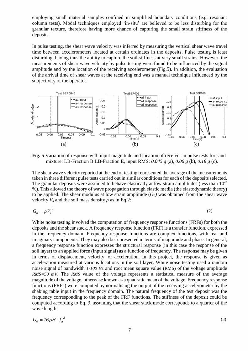
measurements of shear wave velocity by pulse testing were found to be influenced by the signal

amplitude and by the location of the receiving accelerometer (Fig.5). In addition, the evaluation

of the arrival time of shear waves at the receiving end was a manual technique influenced by the

subjectivity of the operator.

(a) (b) (c)

Fig. 5 Variation of response with input magnitude and location of receiver in pulse tests for sand

mixture: LB-Fraction B:LB-Fraction E, input RMS: 0.045 g (a), 0.06 g (b), 0.18 g (c).

The shear wave velocity reported at the end of testing represented the average of the measurements taken in three different pulse tests carried out in similar conditions for each of the deposits selected. The granular deposits were assumed to behave elastically at low strain amplitudes (less than 10-3 %). This allowed the theory of wave propagation through elastic media (the elastodynamic theory) to be applied. The shear modulus at low strain amplitude (G0) was obtained from the shear wave velocity Vs and the soil mass density ρ as in Eq.2:

(2)

White noise testing involved the computation of frequency response functions (FRFs) for both the

deposits and the shear stack. A frequency response function (FRF) is a transfer function, expressed

in the frequency domain. Frequency response functions are complex functions, with real and

imaginary components. They may also be represented in terms of magnitude and phase. In general,

a frequency response function expresses the structural response (in this case the response of the

soil layer) to an applied force (input signal) as a function of frequency. The response may be given

in terms of displacement, velocity, or acceleration. In this project, the response is given as

acceleration measured at various locations in the soil layer. White noise testing used a random

noise signal of bandwidth 1-100 Hz and root mean square value (RMS) of the voltage amplitude

RMS=50 mV. The RMS value of the voltage represents a statistical measure of the average

magnitude of the voltage, otherwise known as a quadratic mean of the voltage. Frequency response

functions (FRFs) were computed by normalising the output of the receiving accelerometer by the

shaking table input in the frequency domain. The natural frequency of the test deposit was the

frequency corresponding to the peak of the FRF functions. The stiffness of the deposit could be

computed according to Eq. 3, assuming that the shear stack mode corresponds to a quarter of the

wave length.

(3)

2

s0 ρVG

2

n

2

0 fH16G

8

0 10 20 30 400

0.5

1

1.5

2

2.5

3 LB- Fraction E

Frequency (Hz)

FR

F M

ag

nitu

de

RMS = 0.05 gRMS = 0.1 gRMS = 0.5 g

z = 0.4 m

0 10 20 30 40 50 600

1

2

3

4

5

Frequency (Hz)

FR

F M

agnitude

Mixure LBFraction B+ LB Fraction E

RMS = 0.03 g

RMS = 0.04 g

RMS = 0.2 g

0 20 40 60 80 1000

0.5

1

1.5

2

2.5

Frequency (Hz)

FR

F M

agnitude

Rubber CT0151

RMS = 0.1 g

RMS = 0.15 g

where H is the height of the shear stack and fn is the natural frequency of the deposit.

By normalising the output of the accelerometers located inside the deposit by the shaking table

input in the frequency domain, the frequency corresponding to the first mode of vibration could

be obtained. As expected, the natural frequency increases from the loose to the dense deposits (fn

= 24 Hz for LB- Fraction E, fn = 32 Hz for the sand mixture LB-Fraction B-LB-Fraction E) (Fig.

6). The natural frequency of the rubber CT0515 layer could not be determined in white noise tests,

as this low density layer became decoupled from the shear stack motion. The shear stack “drives”

the response, therefore the natural frequency of the rubber layer was believed to be lower than the

natural frequency of the shear stack (fn – shear stack= 6 Hz). Similarly to the pulse test results, the

white noise measurements were found to depend on the input magnitude: higher input amplitude

naturally leads to a lower frequency measurement (Fig.6).

Fig.6 FRF (frequency response function) magnitude evolution with increasing input magnitude in

white noise tests (z = 0.4m in the deposit)

Both the pulse and the white noise test measurements were found to be influenced by the position of the accelerometer receiver and by the signal amplitude. In pulse testing the measured shear wave travel time was found to increase with the magnitude of input. Higher magnitude pulses release more energy in the granular texture, being more likely to disturb the initial fabric of the soil. More details on the exploratory tests can be found in [31, 32].

A summary of the average shear wave velocity Vs data obtained in modal tests and of the computed

small strain stiffness values (G0) is shown in Table 5. The values reported for rubber are the ones

obtained in the pulse tests. The values reported for sands represent average results obtained in

pulse and white noise tests. As expected, G0 increases with packing density from rubber CT0515

to the BEE sand mixture.

9

Table 5 Average results from modal testing

3.2 Evaluation of Fundamental Periods for the Deposits

The measured fundamental period values for the decoupled granular layers were employed in the

calculation of the fundamental period of the stratified deposits. The calculation employed an

approximate analytical solution proposed by Hadjian [1] as an enhancement to the Madera

procedure [33]. The Madera procedure consists of replacing the first two layers of an N-layer soil

profile by an equivalent ‘single’ layer. This first equivalent ‘single’ layer and the third layer of the

N-layer profile are then treated as the second two-layer system and, in turn, replaced by an

equivalent single layer. The iterative application of this procedure yields the solution for the

fundamental period of the total soil profile. The Madera procedure is chart based and presents

inaccuracies associated with graphical interpolations between available discrete curves for H1/H2

(Fig.7, H1, H2 = widths of the individual soil layers, T1, T2 = decoupled fundamental periods of the

individual soil layers).

Fig.7 Graphical representation of the fundamental period solution for a two layer system

[1].

The approximate analytical solution proposed by Hadjian [1] increases the calculation accuracy

and can also cater for a variation of density across the soil profile (Eq. 4-6)

n/1

n

22

11

n

1

2

1 H

H1

T

T1

T

T

for 1

H

H

2

1 (4)

2

22

11

H

H2.01

(5)

Modal Test Results Rubber

Particles

CT0515

Sand

LB

Fraction E

Sand

Mixture

LB Fraction B and Fraction E (80:20)

Shear Wave Velocity, Vs (m/s) 14 76 85

Max. Shear Stiffness, G0 (MPa) 0.1 8 14

Fundamental Period, T (s) 0.221 0.043 0.038

Fundamental Frequency, Hz 4.53 23.26 26.32

10

8 10 12 14 16

-0.2

-0.1

0

0.1

0.2

0.3BEE, Sturno A-000, SF=2

Time (s)

Acce

lera

tio

n (

g)

Z=0m

Z=0.2m

Z=0.4m

Z=0.6m

Input10.66 10.68 10.7 10.72 10.74 10.76 10.78

-0.2

-0.1

0

0.1

0.2

BEE, Sturno A-000, SF=2

Time (s)

Acce

lera

tio

n (

g)

Z=0m

Z=0.2m

Z=0.4m

Z=0.6m

Input

2

22

11

H

H8.14n

(6)

where H1 (H2) = height of top (bottom) layer, 1 (2) = density of top (bottom) layer, T1 (T2 )=

decoupled fundamental period of top (bottom) layer, T = fundamental period of the two-layer soil

profile.

The fundamental period values calculated in this study for the ER and the BEE deposits are shown

in Table 6.

Table 6 Calculation of equivalent fundamental period for a 2-layered deposit

It appears that the ER configuration (fER= 4.25 Hz) is less stiff than the shear stack (fshear stack= 6

Hz) and this may trigger the risk of soil decoupling from the enclosing container during dynamic

testing. It is a fundamental requirement that the stack should be ‘softer’ than the deposit in order

for the deposit to drive the response. It is only under these conditions that a realistic recreation of

the soil shearing behaviour can be achieved.

3.3 Seismic Free Field Response

The time histories of the accelerometer signals inside the deposit and on the outside of the shear

stack rings are instrumental in understanding basic aspects of shear wave propagation and motion

coupling under seismic excitation. Figure 8 shows amplitude increase (‘sand column

amplification’) and wave delay as the shear wave travels through the deposit vertically from the

base (z =0.8 m) to the top (z =0 m).

I

(a) (b)

Fig. 8 Free field acceleration response (a-general, b-detail) for BEE soil configuration, input

Sturno-A000, input scale factor SF=2.

Figure 9 shows the outside accelerometer signals and the seismic input being out-of-phase. There

is an expected delay of response as we move upwards from Ring 7 to Ring 1. The BEE granular

deposit and the stack motions are coupled, as revealed by the free surface and the stack’s Ring 1

responses that exhibit a mirror pattern.

Deposit Configuration T1 (s) T2 (s) T/T1 T (s) f(Hz)

ER 0.221 0.043 1.064 0.235 4.25

BEE 0.043 0.038 1.601 0.068 14.52

11

10.3 10.32 10.34 10.36 10.38 10.4-0.2

-0.15

-0.1

-0.05

0

0.05

0.1

0.15Shear Stack, Sturno A000, SF=2

Time (s)

Acce

lera

tio

n (

g)

Ring1

Ring3

Ring5

Ring7

Input

0 20 40 60 80 1001

1.05

1.1

1.15

1.2

1.25

1.3

1.35

1.4BEE Configuration, Sturno A000, SF=2

Frequency(Hz)

FR

F L

ine

ar

Ma

gn

itu

de

Ring1

Ring3

Ring5

Ring7

_________ Inside Soil-------------- Outside Rings

0 20 40 60 80 1001

1.05

1.1

1.15

1.2Monolayer E Configuration, Sturno A000, SF=2

Frequency(Hz)

FR

F L

ine

ar

Ma

gn

itu

de

Ring5

Ring7

_______Inside Soil-----------Outside Rings

Ring3

Ring1

0 20 40 60 80 1001

1.02

1.04

1.06

1.08

1.1

1.12

1.14ER Configuration, Sturno A000, SF=2

Frequency(Hz)

FR

F L

ine

ar

Ma

gn

itu

de

Ring1

Ring3

Ring5

Ring7

0 20 40 60 80 1001

1.05

1.1

1.15

1.2

1.25

Frequency(Hz)

FR

F L

ine

ar

Ma

gn

itu

de

ER Configuration, Inside Stack, Sturno A000, SF=2

z=0 m, Free Surfacez=0.2 mz=0.4 mz=0.6 m

(a) (b)

Fig. 9 Shear stack response (a) and coupling of motions inside and outside the stack (b)

for BEE configuration, Sturno-A000, input scale factor SF=2.

In order to investigate more thoroughly the degree of coupling between the shearing granular

deposits and the container, frequency response functions (FRFs) were computed between the

accelerometer signals and the seismic input at different locations inside and outside the stack.

Figure 10 shows the FRFs inside and outside the shear stack for Sturno-A000 input at a frequency

scaling factor SF=2.

Fig. 10 FRFs outside the shear stack and inside the granular deposits for Sturno-A000

input, input scale factor SF=2 .

The monolayer E deposit moves together with the shear stack in fully coupled motion, displaying

little differences in motion pattern between the inside and the outside of the shear stack. The two-

layer BEE is coupled to the shear stack motion, but the degree of coupling is less pronounced for

the top half of the deposit which has lower stiffness (corresponding to Ring 1 and Ring 3 of the

9.15 9.2 9.25 9.3

-0.15

-0.1

-0.05

0

0.05

0.1

0.15

0.2

BEE, Sturno A-000, SF=2

Time (s)

Acce

lera

tio

n (

g)

Soil Free Surface

Ring1

Soil Free Surface

Ring 1

9.15 9.2 9.25 9.3

-0.15

-0.1

-0.05

0

0.05

0.1

0.15

0.2

BEE, Sturno A-000, SF=2

Time (s)

Acce

lera

tio

n (

g)

Soil Free Surface

Ring1

Soil Free Surface

Ring 1

12

0.8 0.85 0.9 0.95 1

0

0.2

0.4

0.6

0.8

Normalized Mode Shape

Z (

m)

BEE - Outside

BEE - Inside

E - Outside E - Inside

Free Surface

0.95 1 1.05

0

0.1

0.2

0.3

0.4

0.5

0.6

0.7

Normalized Mode Shape

Z(m

)

ER-Outside

ER-Inside

Free Surface

E-Inside

E-Outside

outside response). As for the ER deposit the top half of the stack (Ring 1 and Ring 3) displays a

softer response than the bottom half (Ring 5 and Ring 7) due to the very high stiffness contrast

between the inside granular layers (Gbottom/ Gtop=80). The transfer functions calculated for the

accelerometers located in the top rubber layer (z=0 m and z=0.2 m) do not exhibit any similarities

with the transfer functions calculated for the bottom sand layer. This confirms the fact that the

shearing pattern in the deposit column is interrupted at the interface between the two layers and

that the top half rubber layer becomes decoupled from the shear stack. The free surface of the

rubber layer shows an amplified response and its dynamics is characterized by random large

displacement vibrations on both vertical and horizontal directions. The rubber layer’s low stiffness

is insufficient for driving the stack. In this latter case, the response is driven by the container and

not by the granular deposit. It is thus confirmed that the relative stiffness between stack and the

granular deposit has a paramount influence on the dynamic response and that an accurate

investigation of the free field response requires a soft container and a sufficiently stiff deposit.

The normalized peaks of the Frequency Response Functions (FRFs) were instrumental in

representing the mode shapes of the granular deposit and of the enclosing container, respectively.

The peaks of the FRFs at various ordinates inside and outside the shear stack were normalized

against the maximum value of the FRF for the monolayer E configuration. Comparisons between

the mode shapes for the monolayer E configuration and the bi-layered BEE, and between the

monolayer E and the bi- layered ER are shown in Fig.11a and Fig.11b, respectively. The E and the

BEE configurations show a high degree of coupling between deposit and stack, while the ER

deposit displays a very different shape from the stack mainly because the low stiffness top rubber

layer decouples itself from the stack.

(a) (b)

Fig. 11 Normalized mode shapes for E and BEE deposits (a) and E and ER deposits (b),

respectively, inside and outside the shear stack (Sturno-A000 input, input scale

factor SF=2).

3.4 Dynamic Stiffness Investigation

The stress-strain measurements from the seismic tests were employed in a detailed investigation

of the small strain stiffness of the deposits. The interpretation of the measured dynamic stiffness

was made in relation to the applied dynamic input and to the characteristics of the particulate

materials in the deposits. A classic investigation of shear modulus and damping in soils [10]

illustrated the importance of the set of factors influencing these two dynamic properties (Table 7).

For non-cohesive soils, the relative influence of strain amplitude, effective mean principal stress

and void ratio on dynamic stiffness is known to be very high. It is worth observing that particle

characteristics have both a direct influence, which is ranked as relatively unimportant, and an

indirect influence via the void ratio parameter, whose effect is very strong. One of the objectives

of the present study was to determine the influences of dynamic strain magnitude, initial stiffness

(void ratio) and input frequency content on dynamic stiffness.

13

Table 7 Parameters affecting shear modulus and damping [10]

* V= very important, L= less important, R=relatively unimportant, U=relative importance not clearly known

A pseudo-static free-field response of a soil column to a vertically propagating shear wave is

conceptually represented in Fig. 12. The lateral deflection vectors (ui(t)) are instrumental in

evaluating the shear stress (a-b(t)) and the shear strain (a-b(t)), when the density ( of the deposit

is known (Eqs. 7 and 8).

Fig. 12 Idealized soil response to shearing (ua(t) and ub(t) displacement vectors at two ordinates

inside the deposit)

2/)]t(u)t(u[d)t( abbaba (7)

baabba d/)]t(u)t(u[)t( (8)

In this study, displacement, shear strain and shear stress time histories were evaluated by

integrating the measured acceleration time histories. Cumulative trapezoidal integration was

combined with filtering for elimination of baseline drifts. A high-pass Butterworth filter of 5th

order and a cut-off frequency of 0.5 Hz were employed to eliminate the low-frequency signal

components. The evaluation of strain at the interface between the sandwich layers (z =0.4 m) for

the BEE and the ER deposits, calculated for two different reference ordinates (z =0 m and z =0.2

m, respectively) is shown in Fig. 13. It is interesting to see how the width of the shearing layer

influences the value of the strain magnitude at the interface, according to Eq.7. It was found that

the interface strains calculated against the two selected reference ordinates were of the same order

ua(t)H

L

da-b

ub(t)yy=K0zz

zz=hg

yz=(1/g)zzd2u/dt2

ua(t)H

L

da-b

ub(t)yy=K0zz

zz=hg

yz=(1/g)zzd2u/dt2

Parameter Importance

Modulus Damping

Clean

Sands

Cohesive

Soils

Clean

Sands

Cohesive

Soils

Strain Amplitude V V V V

Effective Mean Principal Stress V V V V

Void Ratio V V V V

Number of Cycles of Loading R R V V

Degree of Saturation R V L U

Overconsolidation Ratio R L R L

Effective Strength Envelope L L L L

Octahedral Shear Stress L L L L

Frequency of Loading (above 0.1 Hz) R R R L

Other Time Effects (Thixotropy_ R L R L

Particle Characteristics (Size, Shape,

Gradation, Mineralogy)

R R R R

Soil Structure R R R R

Volume Change Due to Shear Strain

(for strains less than 0.5%)

U R U R

14

8 10 12 14 16-1

-0.5

0

0.5

1x 10

-3 BEE, Sturno-A000, SF=2

Time (s)

Str

ain

layer: 0.2m - 0.4m

layer: 0m -0.4m

8 9 10 11 12 13 14-2

-1

0

1

2x 10

-3 BEE ,Tolmezzo-A270, SF= 2

Time (s)

Str

ain

layer: 0.2m-0.4m

layer: 0m-0.4m

8 10 12 14 16 18-0.1

-0.05

0

0.05

0.1ER, Sturno-A000, SF=2

Time (s)

Str

ain

layer: 0.2m-0.4m

layer: 0m -0.4 m

8 10 12 14 16 18 20-0.03

-0.02

-0.01

0

0.01

0.02

0.03ER, Tolmezzo-A270, SF=2

Time (s)

Str

ain

layer:0.2m-0.4m

layer:0m-0.4m

of magnitude and displaying a similar pattern for the BEE configuration. However, the interface

strains calculated against the two selected reference ordinates were very different for the ER

deposit. The ER interface strains calculated against the free surface reference level were

unrealistically large, due to the large displacements of the free rubber surface. Therefore, in the

ER case, the free surface could not be taken as a reliable reference for computing strain.

(a) (b)

(c)

(d)

Fig. 13 Strain in soil at interface level (z =0.4 m) for two deposit configurations (BEE (a, b),

ER (c, d) and two seismic inputs (Sturno-A000 (a, c), Tolmezzo-A270 (b, d), SF=2)

A further analysis of dynamic stiffness was carried out by representing the stress-strain loops for

certain cycles extracted from the time histories of the seismic inputs. For example, one of the input

cycles extracted from the Tolmezzo-A270, SF=2 acceleration record is shown in Fig. 14. The

evaluation of the difference in maximum and minimum shear stress applied during a loop, and the

difference in maximum and minimum strain developed in that loop were employed in producing

representative dynamic shear moduli. The dynamic strain () measurements in the seismic tests

ranged up to a maximum value of 0.6 %.

15

-3 -2 -1 0 1

x 10-3

-1500

-1000

-500

0

500

1000

Shear Strain

Sh

ea

r S

tre

ss (

Pa

)

Monolayer E Configuration, Tolmezzo-A270, SF=2

below median line (Z=0.4-0.6 m)

above median line (Z= 0.2-0.4 m)

Gsec-top=0.89 MPat1=10.11 st2=10.5 s

-1 -0.5 0 0.5 1 1.5 2

x 10-3

-600

-400

-200

0

200

400

600

800

1000

1200

Shear Strain

Sh

ea

r S

tre

ss (

Pa

)

Gsec-bottom=1.3 MPat1=11.00 st2=11.32 s

10 15 20 25-0.4

-0.3

-0.2

-0.1

0

0.1

0.2

0.3Base Acceleration Input, Tolmezzo-A270, SF=2

Time (s)

Acce

lera

tio

n (

g)

10.1 10.2 10.3 10.4

-0.3

-0.2

-0.1

0

0.1

0.2

Base Acceleration Input, Tolmezzo- A270, SF=2

Time (s)

Acc

eler

atio

n (g

)

(a) (b)

Fig. 14 Base acceleration input Tolmezzo-A000, SF=2 (a: entire acceleration record,

b: cycle extracted for stress-strain investigation)

Figure 15 shows the hysteretic loop for two different input cycles of the time history. The observed

hysteretic response for the E monolayer configuration shows a small difference in the shear moduli

calculated below and above the interface level (z =0.4 m).

Fig. 15 Observed hysteretic response of soil in the shear stack for monolayer E configuration,

input: Tolmezzo-A270, input scaling factor SF=2 .

The link between the frequency content of the input and the measured dynamic stiffness moduli

was found to be significant. Higher input scaling factors (e.g. SF=12) shifted the earthquakes

energy to the higher frequency range (24-48 Hz). Higher frequency cycling is associated with

higher dynamic stiffness values, which is confirmed in Fig.16. An average stiffness modulus

measured for Sturno-A000, SF=2 was about 2.6 MPa, while the modulus measured at SF=12 was

in the 4-6 MPa range. Both tests employed the same seismic input (same number of loading cycles

N), but different frequency scaling factors (SF).

16

-1.5 -1 -0.5 0 0.5 1 1.5 2

x 10-3

-1500

-1000

-500

0

500

1000

1500

Shear Strain

Sh

ea

r S

tre

ss (

Pa

)

Bilayer BE-E Configuration, Tolmezzo-A270,SF=2

BE- below median line (Z=0.4-0.6 m)

E - above the median line (Z=0.2-0.4 m)

Gsec

1

Gsec-top= 0. 57 MPaGsec-bottom=2.02 MPat1=9.75 st2=10.25 s

-1 -0.5 0 0.5 1

x 10-3

-1000

-500

0

500

1000

1500

Shear Strain

Sh

ea

r S

tre

ss (

Pa

)

Bilayer BE-E Configuration, Tolmezzo-A270, SF=2

Gsec-top=0.89 MPaGsec-botom=2.29 MPat1=10.83 st2=11.05 s

-11 -10 -9 -8 -7

x 10-5

-100

-50

0

50

100

Shear Strain

Sh

ea

r S

tre

ss (

Pa

)

Monolayer E Configuration, Sturno-A000, SF=12

Gsec

1

Z=0.6-0.4m

Gsec=5.76 MPat1=7.45st2=7.50s

3.8 4 4.2 4.4 4.6

x 10-4

-100

-50

0

50

100

150

Shear Strain

Sh

ea

r S

tre

ss (

Pa

)

Monolayer E Configuration, Sturno-A000, SF=12

1

Gsec

Gsec=4.10 MPat1=7.45st2=7.50s

Z=0.4-0.2m

-4 -3 -2 -1 0 1 2

x 10-4

-400

-200

0

200

400

600

Shear Strain

Sh

ea

r S

tre

ss (

Pa

)

Monolayer E Configuration, Sturno-A000, SF=2

Z=0.6 - 0.4 m

Z=0.4 - 0.2 m

1

Gsec

Gsec=2.62 MPa t1=10.32s t2=10.50s

(a)

(b) (c)

Fig. 16 Observed hysteretic response of soil in the shear stack for monolayer E configuration,

input: Sturno-A000, input scaling factor: SF= 2 (a), SF=12 (b, c) .

The dynamic hysteretic response retains some memory of the initial stiffness of the deposit as it

becomes evident for the two layer BEE configuration. Figure 17 shows lower dynamic stiffness

for the lower density layer above the median line (z =0.4 m).

Fig.17 Observed hysteretic response of soil in the shear stack for BEE configuration,

input: Sturno-A000, input scaling factor SF= 2.

The measured dynamic stiffness values for the deposits under selected seismic conditions were

compared to a standard degradation curve for sands [9]. Figure 18 shows that the experimental

values for the monolayer E configuration are in reasonable agreement with the the Seed & Idriss

curve. The dynamic moduli measured for the bottom layer in the BEE double layer configuration

lie slightly lower under the Seed & Idriss curve. Overall, the experimental results increase the

17

N2

v

Seed & Idriss (1970)

S,T,N – RELUIS(2009)

T2 T2

S5

S12

S2

Bilayer: E - top, BE - bottom

BE Shear Stiffness

Go-bottom=14 MPa

N2

v

Seed & Idriss (1970)

v

Seed & Idriss (1970)

S,T,N – RELUIS(2009)

T2 T2

S5

S12

S2

Bilayer: E - top, BE - bottom

BE Shear Stiffness

Go-bottom=14 MPa

N2

v

Seed & Idriss (1970)

S,T,N – RELUIS(2009)

T2

T2

T2

T12

S12

S12

Monolayer E

Go=9 MPa

N2

N2

v

Seed & Idriss (1970)

S,T,N – RELUIS(2009)

T2

T2

T2

T12

S12

S12

Monolayer E

Go=9 MPa

N2

v

Seed & Idriss (1970)

S,T,N – RELUIS(2009)

T2

T2

T2

T12

S12

S12

Monolayer E

Go=9 MPa

v

Seed & Idriss (1970)

v

Seed & Idriss (1970)

S,T,N – RELUIS(2009)

T2

T2

T2

T12

S12

S12

Monolayer E

Go=9 MPa

N2

confidence in the dynamic stiffness measurement techniques associated with the shaking table

testing.

(a) (b)

Fig.18 Dynamic stiffness test results compared with a standard stiffness degradation curve.

Monolayer E (a) and bi-layered BEE (b) deposits. Notation: S (Sturno), T (Tolmezzo),

N (Norcia). Ex: S12 = Test Sturno-A000, input scaling factor SF=12.

4. Concluding remarks

Shaking table test results of granular materials sheared in plane strain conditions in a large uniaxial

shear stack were reported. The shear stress-strain behaviour of three configurations (one witness

mono-layered deposit and two bi-layered deposits) was analysed under a set of seismic inputs with

different frequency content. Two modal testing techniques (i.e. pulse testing and random white

noise testing) were successful in measuring the fundamental periods of the individual layers. The

measured fundamental periods of the decoupled granular layers were employed in the calculation

of the equivalent fundamental period of the bi- layered deposits by an enhanced Madera procedure

([1]).

The dynamics of the granular deposits was analysed in relation to the inherent stiffness the shear

stack, the particulate material characteristics and the dynamic input parameters. The initial

stiffness of the test deposits was mainly influenced by the packing density for sands (E and BEE

configurations) and by the packing density and particle intrinsic stiffness for the rubber layer. The

sand deposits (mono-layered E and the bi- layered BEE) drove the shearing response of the shear

stack and exhibited motion coupling inside and outside the shear stack across the vertical direction.

The ER configuration that consisted of rubber granules in its top layer was found to exhibit a lower

fundamental frequency than the shear stack (fER= 4.25 Hz, fshear stack= 6 Hz), therefore its

decoupling from the enclosing container during seismic testing was understood. The free surface

measurements for the ER configuration were unreliable in strain calculations.

The dynamic hysteretic loops obtained in the experiments show some memory of the initial

stiffness of the deposits, as it became evident for the two layered BEE configuration (higher secant

stiffness for the dense/stiff bottom layer). The analysis of the hysteretic response of sands and the

frequency content of the seismic input shows that higher frequency (24-48 Hz) loading cycles

resulted in higher values of measured dynamic stiffness in both the monolayer and the stratified

deposits. The shear stress-shear strain results for the mono-layered and the bi-layered sand deposits

compare well with previous commonly-used empirical curves for sands [9], increasing the

18

confidence in the shaking table and shear stack testing for the dynamic investigation of granular

media.

Acknowledgements

The financial support from ReLUIS (Rete di Laboratori Universitari Ingegneria Seismica) for

conducting this research is gratefully acknowledged. The authors would like to thank Eleonora

Iannacce and Domenico Lombardi for their contribution to the experimental work and to Professor

David Muir Wood for his advice on granular material testing.

References

[1] Hadjian, A.H. Fundamental period and mode shape of layered soil profiles. Soil Dyn

Earthquake Eng 2002; 22: 885-91.

[2] Gazetas G. Soil dynamics: an overview. In: Banerjee P.K. & Butterfield R., editors. Dynamic

behaviour of foundations and buried structures. Elsevier Science Publishing Co., 1987

[3] Novak M. Experimental studies of the dynamic behaviour of piles and pile groups. In: Banerjee

P.K. & Butterfield R., editors. Dynamic behaviour of foundations and buried structures. Elsevier

Science Publishing Co., 1987.

[4] Badoni D., Makris N. Nonlinear response of single piles under lateral inertial and seismic

loads. Soil Dyn Earthquake Eng 1996; 15: 29-43.

[5] Tokimatsu K., Mizuno H., Kakurai M. Building damage associated with geotechnical

problems. Special issue Soils and Foundations, Japanese Geotechnical Society, 1996; Jan: 219-34.

[6] Mylonakis G., Nikolaou A., Gazetas G. Soil-pile-bridge seismic interaction: kinematic and

inertial effects. Earthquake Eng Struct Dyn 1997; 26:337-59.

[7] Bhattacharya S.A Review of methods for pile design in seismically liquefiable soils. In:

Bhattacharya S., editor. Design of foundations in seismic areas: principles and applications.

National Information Centre of Earthquake Engineering. Indian Institute of Technology,

Kanpur,ISBN 81-904190-1-3, 2007.

[8] Richart, F.E, Jr., Hall, J.R., Jr., Woods, R.D. Vibrations of soils and foundations. Prentice-Hall,

Englewood Cliffs, N.J.;1970.

[9] Seed, H.B., Idriss, I.M. Soil moduli and damping factors for dynamic response analysis. Rep.

No. EERC 70-10. Earthquake Engineering Research Centre, Berkeley, CA.; 1970.

[10] Hardin, B.O., Drnevich, V.P. Shear modulus and damping in soils. J. Soils Mech. Found. Div.

1972a; 98(7):667-92.

[11] Vucetic, M., Dobry, R. Effect of soil plasticity on cyclic response. J. Geotech. Eng. 1991;

117(1):89-107.

[12] Ishibashi, I., Zhang, X.J. Unified dynamic shear moduli and damping ratios of sand and clay.

Soils Found. 1993; 33(1):182-91.

[13] Darendelli, M.B. Development of a new family of normalized modulus reduction and material

damping curves. PhD thesis. Univ. of Texas at Austin, Austin, TX; 2001.

19

[14] Ohtsuki A., Hirota M., Ishimura K., Yokoyama K., Fukutake K. Verification of two-

dimensional non-linear analysis of sand-structure system by examining the results of the shaking-

table test. Earthquake Eng & Structural Dynamics, 1992, 21(7); 591-607.

[15] Meymand P.J. Shaking table scale model tests of nonlinear soil-pile-superstructure interaction

in soft clay. Ph.D.thesis. Berkeley, CA: The University of California, Berkeley, 1998.

[16] Prasad S.K., Towhata I., Chandradhara G.P., Nanjunaswamy P. Shaking table tests in

earthquake geotechnical engineering. Curr Sci 2004; 87 (10):1398-404.

[17] Tokimatsu K., Susuki, H. Effect of inertial and kinematic interactions on seismic behaviour

of pile foundations based on large shaking table tests. Proc. 2nd CUEE Conf. Urban Earthquake

Eng, Tokio Institute of Technology, 2005.

[18] Pitilakis D., Dietz M, Muir Wood D., Clouteau D., Modaressi A. Numerical simulation of

dynamic soil-structure interaction in shaking table testing. Soil Dyn Earthquake Eng 2008; 28:

453-67.

[19] Takahashi A., Takemura J., Susuki A., Kusakabe O. Development and performance of an

active type shear box in a centrifuge. Int. J. Phys. Model Geotech 2001; 1(2):1-18.

[20] Dar A.R. Development of a flexible shear stack for shaking table testing of geotechnical

problems. PhD Thesis, University of Bristol, 1993.

[21] Fishman K.L., Mander J.B. & Richards R. Laboratory study of seismic free-field response of

sand. Soil Dyn Earthquake Eng 1995; 14: 33-43.

[22] Gibson A.D. Physical scale modelling of geotechnical structures at one-g. Ph.D.thesis.

Pasadena, CA: California Institute of Technology; 1997.

[23] Turan A., Hinchberger S., Naggar H.E. Design and commissioning of a laminar soil container

for use on small shaking tables. Soil Dyn Earthquake Eng 2009; 29: 404-14.

[24] Ashford, S. and Jakrapiyam, W. Design and verification of the UCSD laminar container.

SSRP 2001-07, University of California, San Diego; 2001.

[25] Thevanayagam, S. et al. Laminar Box System for 1-g Physical Modeling of Liquefaction and

Lateral Spreading", Geotechnical Testing Journal 2009; 32(5).

[26] Chang, B.J., and Hutchinson, T.C..Experimetnal evaluation of p-y curves considering

liquefaction development. SSRP-09/13, University of California, San Diego; 2010.

[27] Crewe A.J., Lings M.L., Taylor C.A., Yeung A.K., Andrighetto R. Development of a large

flexible shear stack for testing dry sand and simple direct foundations on the shaking table. In:

Elnashai, editor. European seismic design practice. Rotterdam: Balkema; 1995.

[28] German R. Particle Packing Characteristics, Metal Powder Industries Federation, New

Jersey;1989.

[29] Roberts M. J. Signals and systems: analysis using transform methods and MATLAB.

McGraw-Hill Professional. ISBN 0072499427; 2004

20

[30] Blackledge J.M. Digital signal processing: mathematical and computational methods,

software development and applications. Horwood Publishing. ISBN 1898563489; 2003

[31] Dihoru, L., Bhattacharya, S., Taylor, C.A., Muir Wood, D., Moccia, F., Simonelli, A.L. &

Mylonakis, G.. Experi mental modelling of kinematic bending moments of piles in layered soils.

In (Eds) Kokusho, Tsukamoto & Yoshimine, Proc. Performance-based design in earthquake

geotechnical engineering, Tokio, Japan, 2009.

[32] Moccia F. Seismic soil pile interaction: experimental evidence. PhD.thesis. Naples, IT:

Università degli studi di Napoli ‘Federico II’, 2010.

[33] Madera, G.A. Fundamental period and amplification of peak acceleration in layered systems.

Research Report R 70-37, June. Cambridge, MA: MIT Press; 1970.