~ear Observational Equivalence

and

Persistence

by Stephe~ R. BIo~gh

©

~ear ObservationalE’quwalence

Persistence in G~%~P

by Stephen R. Blough

December 1994Working Paper No. 94-6

Federal Reserve Bank of Boston

Near Observational Equivalence and Persistence in GNP

Stephen R. Blough"

October 1994

"Research Department, Federal Reserve Bank of Boston, Boston, MA 02106-2076. I amindebted to Alicia Sasser for research assistance, and to Jeff Fuhrer for comments. This paperis a substantially revised and abridged version of Blough (1992b), which was written at JohnsHopkins University. The views in this paper are not necessarily endorsed by the Federal ReserveBank of BoSton or the Federal Reserve System.

The question of whether aggregate output is best described as a trend-stationary (TS) or

as a difference-stationary (DS, or un1~ root) process continues to generate a substantial volume

of research a dozen years after i~ was first raised by Nelson and Plosser (1982), including a recen~

paper by Rudebusch (1993). Rudebusch argues that "Based on the usual unit root tests, little can

be said about the relative likelihood of the specific DS and TS models of real GNP." Rudebusch

concludes by emphasizing "the importance of measuring the confidence intervals for estimates

of persistence without conditioning on the TS or DS modeI."

This paper provides a strong theoretical result on distinguishing TS and DS models, and

gives confidence intervals for the GNP impulse response function that do not require such

distinction. Theoretically, the paper shows that, in the absence of a prior~ specification

restrictions, the classes of unit root and stationary processes are nearly observationally equivalent:

no finite data sample can provide information on the TS/DS issue. The paper then shows how

the principle of parsimony for time series model specification masks near observational

equivalence and implicitly rules out plausible shapes for the univariate impulse response function.

Finally, the paper provides confidence intervals for the GNP impulse response function using two

methods that nest parslmonious TS and DS models.

1. Near Observational Equivalence.

The classes of unit root and stationary processes are nearly observationally equivalent in

that any finite sample, finite horizon, or discounted infinite horizon behavior of any member of

either class of processes can be arbitrarily well approximated by members of the other class. To

see this, consider processes of the form:

(~)

where {et} is a white noise process, L is the lag operator, pand 0are each less than or equal to

one in absolute value, and b(L) is a lag polynomial of possibly infinite length whose roots lie

entirely outside the unit circle and whose coefficients are square summable. Observations of {y.~}

are available for t=l,...,T. So that the observations have a will-defined unconditional distribution

in the unit root case/7=1, the process is assumed to-have start date s with initial value y, drawn

from some proper distribution function S(.). All results are unchanged if {Yt} contains arbitrary

deterministic components, such as time trends; these are omitted from the representation for

notational compacmess.

Representation (1) nests the Wold representations of all stationary processes (when p= 0=0)

and of all difference stationary processes (when ,o=1 and 6a:0). The process {yt} is stationary for

all t,d<l. Fixing p=l,. {Yt} has a unit root for all 0~-1, while for 0=-1 the roots cancel and {yt}

is again stationary.

Near observational equivalence is shown by examining sequences of processes while

keeping sample size fixed (in contrast to increasing sample size while keeping the process fixed,

as in asymptotic theory). Equation (1) gives each observation y, as a function of the parameters

(p,O,b(L)) and the realization of the random variables ~- (y, ; g t=s+l,...,T). Denote by

{y,(p,O,b(L))}r a sample of length T from a process (1), with dependence on ~ understood.

Then for fixed values of 0 and b(L), a sequence of processes is implied by a sequence of

values 6f ,o. Consider in particular sequences of the form:

lim p~ = l

(2)

Each process in this sequence is stationary, while the limiting process has a unit root. It is

essential to note that the limiting process can be any unit root p~ocess by appropriate choice of

Conversely, fixing p and b(L), a sequence of values of Oimplies a sequence of processes.

All processes in the sequence:

~ >-1 Vilim 0, = - 1

have a unit root. However, the limiting process is {yt(1,-1,b(L))}, which by cancellation of the

roots is the stationary process {y,(0,0,b(L))}. Again, note that appropriate choice of b(L) permits

the limiting process of a sequence (3) to be any stationary process.

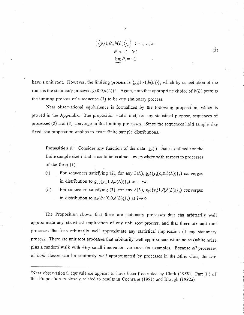
Near observational equivalence is formalized by the following proposition, which is

proved in the Appendix. The proposition states that, for any statistical purpose, sequences of

processes (2) and (3) converge to the limiting processes. Since the sequences hold sample size

fixed, the proposition applies to exact finite sample distributions.

Proposition 1.~ Consider any function of the data gr(.) that is defined for the

finite sample size T and is continuous almost everywhere with respect to processes

of the form (1).

(i) For sequences satisfying (2), for any b(L), gr({yt(p~,O,b(L))}r) converges

in distribution to gr({yt(1,O,b(L))}r) as

(ii) For sequences satisfying (3), for any b(L), gr({Yt(1,Oi,b(L))}r) converges

in distribution to gr({yt(O,O,b(L))}r) as

The Proposition shows that there are stationary processes that can arbitrarily well

approximate any statistical implication of any unit root process, and that there are unit root

processes that can arbitrarily well approximate any statistical implication of any stationary

process. There are unit root processes that arbitrarily well approximate white noise (white noise

plus a random walk with very small innovation variance, for example). Because all processes

of both classes can be arbitrarily well approximated by processes in the other class, the two

~Near observational equivalence appears to have been first noted by Clark (1988). Part (ii) Ofthis Proposition is closely related to results in Cochrane (1991) and Blough (1992a).

4

classes are nearly observationally equivalent.’- No statistical procedure can meaningfully.

discriminate between them)

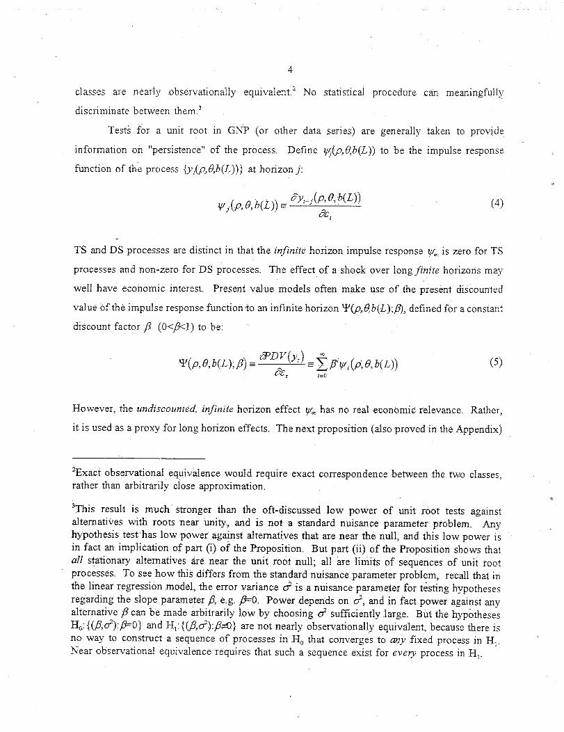
Tests for a umt root in GNP (or other data series) are generally taken to provide

information on "persistence" of the process Define ~.(~9,0,b(L)) to be the impulse response

function of the process {yt(p,O,b(L))} at horizon j:

=

TS and DS processes are distinct in that the in.finite horizon impulse response y~ is zero for TS

processes and non-zero for DS processes. The effect of a shock over long finite horizons may

well have economic interest. Present value models often make use of the present discounted

value Of the impulse response function to an infinite horizon ~Y(,o,0,b(L);fl), defined for a constant

discount factor fl (0<fl<l) to be:

However, the undiscounted, infinite horizon effect ~o has no real economic relevance. Rather,

it is used as a proxy for long horizon effects. The next proposition (also proved in the Appendix)

2Exact observational equivalence would require exact correspondence between the two classes,rather than arbitrarily close approximation.

~This result is much stronger than the off-discussed low power of unit root tests againstalternatives with roots near unity, and is not a standard nuisance parameter problem. Anyhypothesis test’has low power against alternatives that are near the null, and this low power isin fact an implication of part (i) of the Proposition. But part (ii) of the Proposition shows thatall stationary alternatives are near the unit root null; all are limits of sequences of unit rootprocesses. To see how this differs from the standard nuisance parameter problem, recall that inthe linear regression .model, the error variance ~ is a nuisance parameter for t~sting hypothesesregarding the slope parameter fl, e.g. fl=0. Power depends on ~, and in fact power against anyalternative fl can b-e made arbitrarily low by choosing ~ sufficiently large. But the hypothesesH0: {(f!,c?):fl=0} and H~: {(fl, d):fl~0} are not nearly observationally equivalent, because there isno way to construct a sequence of processes in H0 that converges to any fixed process in H~.Near observational equivalence requires that such a sequence exist for every process in H~.

shows that this use is not justified in the general case: the presence or absence of a unit root has

no implications for the impulse response function m any finite horizon, nor for the discounted

infinite horizon impulse response function at any positive discount rate.

Proposition 2. (i) Along the sequences defined by (2), for all finite.i:

lim ~j(p,,0,b(L))= ~j (1,0, b(L))

li_,m~ W(p~,O, b(L); 13) = q~(1, 0, b(L );/3)(6)

(ii) Along sequences defined by (3), for all finite j:

!ira ~j.(1,0~,b(L))= ~j(0,0, b(L))

0i, b(z); 13) = b(L); 13)(7)

Any property of the impulse response function except the undiscounted infinite horizon

can be produced, to an arbitrarily accurate approximation, by either a stationary or a unit root

process. Even if the data could provide information on the presence or absence of a unit root,

that information by itself would have no implications about the behavior of the process over any

relevant horizon. Recognition of near observational equivalence therefore strengthens the

conclusion of Christiano and Eichenbaum (1990), who ask, "Unit roots in GNP: do we know and

do we care?" and answer, "No, and maybe not." The results in this section imply in fact that we

cannot know and we should not care,

2. The Principle of Parsimony and Estimates of Persistence.

It is tempting to dismiss near observational equivalence as unimportant for practical

purposes. The unit root processes that closely approximate a given stationary process for

statistical purposes (Proposition l(ii)) are those that closely approximate the finite horizon

impulse responsefunction of that stationary process (Proposition 2(ii)).4 Why then worry about

the fact that such processes cannot be distinguished?s

This approach is unsatisfactory for two reasons. First, it leaves unspecified the question

being addressed by a unit root test. For a given purpose, nearly stationary unit root processes

may well be appropriately classed together with the associated stationary process, and stationary

processes with roots near one classed wi~h the associated unit root process. But what defines the

two classes? Once the literal distinction between TS and DS processes is abandoned, as required

by near observational equivalence, what definition of persistence" is put in its place, and how

much of it must a process have to be classified as having a "unit root"? Are different definitions

appropriate for different purposes? How do the properties of various unit root tests relate to these

definitions?6

Second, treatment of TS and DS processes as distinct classes, combined with the standard

principle of parsimony for time series specification, has discouraged nested analysis of the types

of finite sample persistence about which the data can be informative. This problem is best

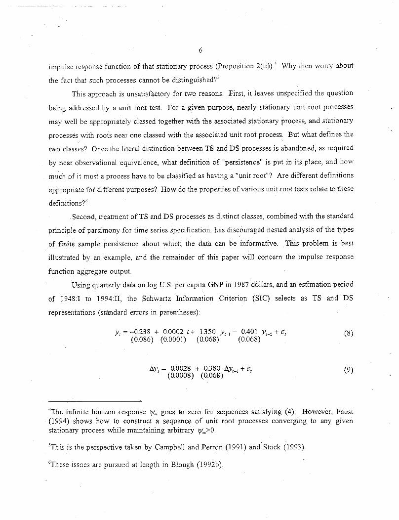
illustrated by an example, and the remainder of this paper will concern the impulse response

function aggregate output.

Using quarterly data on log U.S. per capita GN-P in 1987 dollars, and an estimation period

of 1948:I to 1994:II, the Schwartz Information Criterion (SIC) selects as TS and DS

representations (standard errors in parentheses):

Yt =-0.238 + 0.0002 t+ 1.350 Yt-1- 0.401 Yt-2 + s, (8)(0:086) (0.0001) (0.068) (0.068)

Ayz = 0.0028 + 0.380l~yt_1 "k~t (9)(0.O00S) (0.068)

~The infinite horizon response q/~ goes to zero for sequences satisfying (4). However, Faust(1994) shows how to construct a sequence of unit root processes converging to any givenstationary process while maintaining arbitrary ~>0.

SThis is the perspective taken by Campbdl and Perr0n (1991) and Stock (1993).

6These issues are pursued at length in Blough (!992b).

7

The estimates are very similar to those obtained by Rudebusch (1993) using a somewha~ shorter

sample. Omitting the constant and trend terms, both specifications can be written in the form:

(lo)

where the minor autoregressive root P2 is 0.442 in the TS specification (8) and 0.380 in the DS

specification (9). The long-run properties of the processes are determined by the dominant root

Pl, which is estimated to be 0.908 in the TS model and fixed at one in the DS model.

The impulse response functions of the two specifications are plotted as the solid lines in

Figure 1. They differ dramatically after only a few quarters: the TS impuIse response peaks in

the second quarter after an innovation and has fallen to 0.5 after 12 quarters on its way to zero;

the DS impulse response increases monotonically, nearing its asymptonc value of 1.6 by the time

six quarters have passed. These striking differences monvate the use of unit root tests to choose

between the two specifications.

Equation (10) nests the TS and DS models; given the minor root p2, confidence intervals

for the impulse response function ~ to any finite horizon i could be formed from a confidence

interval for Pi- This approach will be pursued in the next section. However, this procedure is

unsatisfactory if persistence is measured by the infinite horizon response: ~’, is zero for any

p~<l, but equal to 1/(1- p~) when pl=l. Variation of p~ does vary ~, but, as noted by

Cochrane (1988) and Christiano and Eichenbaum (1990), this rom is determined by the short

horizon properties of the process. In practice th£ infinite horizon responses of the TS and DS

models are not nested in the specification (10).

A nesting that allows for a continuum of values of V~ may be achieved by dropping the

principle of parsimony to allow near common autoregressive and moving average factors. In the

representation:

0 - P3I-’)(1 - lOlL )ky~ = (1 + 0/; )g,

the long-run effect of a shock is given by:

(11)

(1+0) 1 (12)~’* = (l-p3) (l-p:)

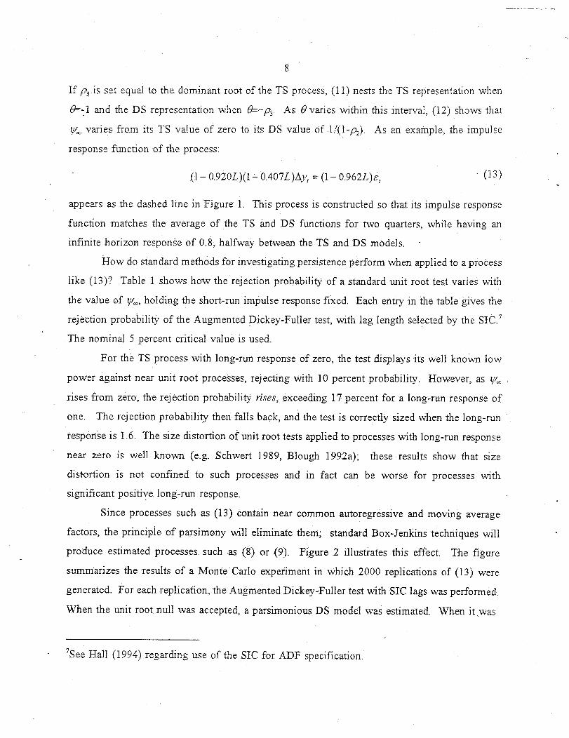
If P3 is set equal to the dominant root of the TS process, (11) nests the TS representation when

0=-1 and the DS representa’fion when 0=-p> As 0 varies w~thin this interval, (12) shows that

V, varies from its TS value of zero to its DS value of 1/(1-/92). As an example, the impulse

response function of the process:

(1- 0.920/.)(1 a 0.407L)zXyt = (1- 0.962L)c,(I3)

appears as the dashed line in Figure 1. This process is constructed so that its impulse response

function matches the average of the TS and DS functions for two quarters, while having an

infinite horizon response of 0.8, halfway between the TS and DS models.

How do standard methods for investigating persistence perform when applied to a process

like (13)? Table 1 shows how the rejection probability of a standard unit root test varies with

the value of V~, holding the short-run impulse response fixed. Each entry in the table gives the

rejection probability of the Augmented Dickey-Fuller test, with lag length selected by the SIC.7

The nominal 5 percent critical value is used.

For the TS process with long-run response of zero, the test displays its well known low

power against near unit root processes, rejecting with 10 percent probability. However, as ~

rises from zero, the rejection probability rises, exceeding 17 percent for a long-run response of

one. The rejection probability then falls back, and the test is correctly sized when the long-run

response is 1 °6. The size distortion of unit root tests applied to processes with long-run response

near zero is well known (e.g. Schwert 1989, Blough 1992a); these results show that size

distortion is not confined to such processes and in fact can be worse for processes with

significant positive long-run response.

Since processes such as (13) Contain near common autoregressive and moving average

factors, the principle of parsimony will eliminate them; standard Box-Jenkins techniques will

produce estimated processes such as (8) or (9). Figure 2 illustrates this effect. The figure

summarizes the results of a Monte-Carlo experiment in which 2000 replications of (13) were

generated. For each replication, the Augmented Di ckey-Fuller test with SIC lags was performed.

When the unit root null was accepted, a parsimonious DS model was estimated. When it,was

7See Hall (1994) regarding use of the SIC for ADF specification.

9

Table 1

ADF-SIC Rejection Probabilities for Simulated GNP Processes

(2000 replications. Standard errors in parentheses.)

Infinite Horizon Response

0 0.2 0.4 0.6 0.8 1.0 1.2 1.4 1.6

0.107 0.149 0.165 0.170 0.168 0.179 0.142 0.090 0.052

(0.007) (0.008) (0.008) (0.008) (0.008) (0.009) (0.008) (0.006) (0.005)

Source: Simulations by author. For each entry except "1.6", the parameters of an ARIMA(2,1,1) model were chosenso as to give the indicated value of the infinite horizon response, while maintaining one- and two-period impulseresponses equal to the average of those for TS and DS specifications estimated on log per capita GNP data (seetext). For "1.6", an ARI(1,1) process was used with autoregressive parameter 0.375. For each replication for eachprocess, 2i6 observations were produced The first 20 observations were discarded and 10 observations werereserved for lags, leaving a sample of 186 to match the GN-P data. The Augmented Dickey-Fuller test statistic wascalculated, with Constant and trend included and with order chosen by the SIC. Table entries are fraction ofreplications with the test statistic less than the nominal 5 percem critical value (-3.44). Computations wereperformed in GAUSS.

rejected, a parsimonious TS model was estimated. Figure 2 plots the 95 percent ranges for the

two resulting groups of estimated impulse response functions. After 12 quarters, neither band

includes the true impulse response function. Standard estimation procedure will either greatly

overstate or greatly understate the long-run persistence of this process.

3. Results for nested models.

This section presents the results of two methods for estimating impulse response functions

for GNP that nest the parsimonious TS and DS models. The two methods correspond to the two

nested representations (10) and (11).8

8Fractionally integrated (ARFIMA) models also nest trend- and difference-stationaritv. Dieboldand Rudebusch (1989) present ARFIMA estimates for the impulse response function of aggregateoutput. Their results agree qualitatively with those presented below: confidence bands are wide.

10

The first method is an extension of the "root local to unity" (RLU) confidence intervals

developed by Stock (1991) for the dominant roo~ in a time series. Rewrite (10) as:

(1- p2)(1- (1-+ c/T)L)y, = e, (14)

where T is the number of observations. Stock shows how to use asymptotic theory to construct

a confidence interval for c from the Augmented Dickey-Fuller t-statistic. If the minor root t92 is

treated as fixed, the impulse response function of (14) to any horizon is monotonically related

to c. Upper and lower confidence bounds for the impulse response function may be obtained

using the endpoints of the confidence interva! for c in (14). DS processes correspond to c=0, TS

processes to c<0. The confidence imerva! may also include explosive roots (c>0), in which case

the upper confidence bound for the impulse response function wilt diverge. Treating P2 as fixed

imparts a conservative bias to the confidence bounds.

While the RLU confidence bands so constructed can nest the TS and DS impulse

responses to any finite horizon, the procedure does not produce a confidence interval for the

infinite horizon response. W, is zero for c<0, 1/(l-p2) for c=0, and oo for c>0. This occurs

because DS processes appear as a single point in (10). The near common factor nesting (11)

includes a continuum of DS processes, and therefore confidence regions for its parameters imply

confidence intervals for

Estimation of (11) confronts the well-known problems Of estimation with near common

factors and near unit moving average roots. Parameter estimates have very badly behaved

distributions, and standard procedures for constructing confidence regions give extremely

unreliable results. Blough (1994) surveys these problems and proposes a solution. Again treating

The ARFIMA method is not pursued here, for the following reason. An ARFIMA model thatnests.the parsimonious TS and DS representations is (1-p3L)(1-paL)(1-L)dyt=~ , where d is thedifferencing parameter which may take values on the real line. The TS model (8) correspondsto p3=0.908, d=0, while the DS model (10) corresponds to p~=0, d=l. Formation of a jointconfidence region for (p~,d) is problematic, however. The points (1,0) and (0,1) are equivalent,meaning that a proper confidence region cannot be elliptical and may be disjoint. Diebold andRudebusch avoid this problem by, in effect, setting p~=0 and using d alone to determine the lowfrequency behavior of the process. For this reason, the parsimonious TS model is not nested intheir specification.

11

the minor root P2 as fixed, the likelihood function is evaluated at all points on a grid of values

of (p3,(?). A "likelihood ratio confidence region" (LRCR) for these two parameters is defined as

the set of values of (/93,0) that are not rejected by a likelihood ratio test. Monte Carlo evidence

indicates that the LRCR has good properties for sample sizes typical of post war quarterly data.

Note that adequacy of the parsimonious DS process (9) implies that-the common factor line/93=-(9

will be included in the LRCR. Continuity of the likelihood function implies that points near that

line, e.g. with P3 and -0 both near one, will be included as well.

Each accepted value of (P3,0) implies an impulse response function for {Yt}~ Confidence

bounds for the impulse response function at a given horizon are given by the minimum and

maximum of the impulse response function of (11) at that horizon over the values of (/93,0) in

the LRCR. As with the RLU, treating P2 as fixed imparts a conservative bias.

Figure 3 shows the RLU and LRCR 95 percent confidence bounds for the GNP impulse

response function. For both procedures, the minor root/93 is fixed at 0.41, the average of its

values in the parsimonious TS and DS specifications (8) and (9). The Dickey-Fuller t-statistic

for the quasi-differenced process {yt-0.41yt4} is -2.83, giving a 95 percent confidence interval

of [-17,2] for the local-to-unity parameter c using Figure 2 of Stock (1991). The implied 95

percent confidence interval for p~ is [0.909, 1.011]. The LRCR bounds are generated by

evaluating the likelihood function over the grid

p3 ~ {-0.99, - 0.95, - 0.90,..., 0.90, 0.95, 0.99}

0 ~ {1, - 0.99, - 0.95, - 0.90 .... ,0.90, 0.95, 0.99, 1}(]5)

While the LRCR bounds for the impulse response function may correspond to different processes

for different horizons, for the most part the upper bound corresponds to (p~,0)=(0.70,-0.65),

while the lower bound corresponds to (0.85,-0.99) out to 24 quarters, and to (0.90,-1) thereafter.

The 95 percent confidence bounds are wide: there is very little information in postwar

data about the univariate impulse response function of real GN-P beyond a very few quarters.

Even at a horizon of eight quarters, the confidence interval is roughly (0.7, 1.8); at 20 quarters,

it is about (0.25, 2). The LRCR gives a 95 percent Confidence interval for ~’~ of (0, 1.98), while

the RLU indicates that an explosive root cannot be ruled out.

12

The differences between the RLU and the LRCR bounds can be explained by differences

in specification restrictions and in finite sample performance. For the upper bound, the allowance

-of a moving average factor in the LRCR dominates in the .early quarters, while the explosive root

in the RLU dominates for longer horizons. The lower bounds differ largely because of opposite

finite sample biases. The Monte Carlo experiments in Stock indicate that the confidence interval

of c is rather conservative (with T=200 and c=-10, the true value is covered by a nominal 95

percent confidence interval with 91 percent probability), While a simulation of the LRCR shows

that it is somewhat liberal in this region.9

4. Concluding remarks.

The question of whether or not there is a unit root in real GNP, or in any other macro

time series, is ill-defined. The classes of unit root and stationary processes are not meaningfully

distinct in the absence of a priori specification restrictions. If the TS / DS distinction is meant

to be a proxy for the long finite horizon properties of the impulse response function,

understanding -would be better served by stating the properties of interest directly and developing

methods of inference about them that are robust to statistical specification. The examples of this

approach presented here provide explicit measurements of the uncertainty about GNP persistence.

These points have obvious implications for multivariate analysis. Nothing about

Propositions 1 and 2 requires {Yt} to be a univariate process, and the extension to cointegration

is straightforward.~° Thus, multivariate impulse response functions that are sensitive to assumed

orders of integratmn should be interpreted carefully. Multivariate methods for nesting

specifications would be very useful for dealing with these issues.

~With T=185 and 1000 replications, the process p2=0.85 and 0=-0.99 is covered by a nominal 95percent LRCR with 97 percent probability.

~°See Btough (1992b).

Appendix.

13

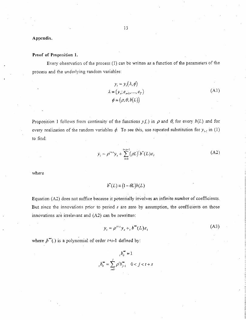
Proof of Proposition 1.

Every observation of the process (1) can b~ written as a function of the parameters of the

process and the underlying random variables:

Yt = Y,(A,O)

-= (A1)

Proposition 1 follows from continuity of the functions y,(.) in p and 0, for every b(L) and for

every realization of the random variables ~. To see this, use repeated substitution for Yt-1 in (1)

to find:

t+s-1

y, = p y, ~_ ~, (pL)ib’(L)g, (A2)

where

Equation (A2) does not suffice because it potentially involves an infinite number of coefficients.

But since the innovations prior to period s are zero by assumption, the coefficients on those

innovations are irrelevant and (A2) can be rewritten:

~+" +t b’*(L)e~y¢ = p

where ])*’(.) is a po!yn£mial of order t+s-1 defined by:

(A3)

tbo =1

i=0

14

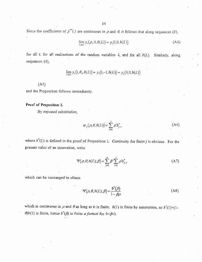
Since the coefficients of ,b"(.) are continuous in p and 0, it follows that along sequences (3),

li+m~ y~(p~,O,b(L))= y~(1,0, b(Z)) (A4)

for al! t, for all realizations of the random variables 2, and for all b(L).

sequences (4),

lim y,(1,0,,b(L))= y,(1,-1,b(L))= yt(O,O,b(L))

Similarly, along

(AS)and the Proposition follows immediately.

Proof of Proposition 2.

By repeated substitution,

i=0

where b’(L) is defined in the proof Of Proposition 1. Continuity for finitej is obVious. For the

present value of an innovation, write

which can be rearranged to obtain

(AS)

which is continuous in p and O as long as it is finite; b(1) is finite by assumption, so b’(1)=(1-

8)b(1) is finite, hence b’(/5) is finite afortiori for 0</?<1.

15

References

B10ugh, Stephen R., "The Relationship Between Power and Level for Generic Unit Root Tests

in Finite Samples, Journal of Applied Econometrics, July-September 1992a, 3, 295-308.

__., "Near Observational Equivalence of Unit Root and Stationary Processes: Theory and

Implications," wprking paper, Johns Hopkins University, 1992b.

__., "Near Common Factors and Confidence Regions for Present Value Models," Working

Paper no. 94-3, Federal Reserve Bank of Boston, 1994.

Campbell, John Y. and Pert’on, Pierre, "Pitfalls and Opportunities: What Macroeconomists

Should Know About Unit Roots," N~3ER Macroeconomics Annual, 1991, 143-201.

Christiano, Lawrence J. and Eichenbaum, Martin, "Unit Roots in Real GNP: Do We Know, and

Do We Care?" Carnegie-Rochester Conference Series on Public _Policy, Spring 1990, 7-62

Clark, Peter K,, "Nearly Redundant Parameters and Measures of Persistence in Time Series,"

Journal of Economic Dynam its and Control, June!September- 1988, 12, 447-461.

Cochrane, John H., "How Big is the Unit Root in GN-P?" Journal of Politica! Economy, October

1988, 96, 893-920.

~., "A Critique of the Application of Unit Root Tests," Journal of Economic Dynamics and

Control° 1991, 15, 275-284.

Diebold, Francis X. and Rudebusch, Glenn D., "Long Memory and Persistence in Aggregate

Output," Journal of Monetary Economics, September 1989, 24, 189-209.

Faust, Jon, "Near Observational Equivalence and Unit Root Processes: Formal Concepts and

Implications," working paper, Federal Reserve Board, 1994.

Hall, Alastair, "Testing for a Unit Root in Time Series with Pretest Data-Based Model Selection,"

Journal of Business & Economic Statistics, October 1994, 12, 1-10.

Nelson, Charles R. and Plosser, Charles L, "Trends and Random Walks in Macroeconomic Time

Seriesi Some Evidence and Implications," Journal of Monetary Economics, September 1982, lO,

139-62.

Rudebusch, Glenn D., "The Uncertain Unit Root in Real GN-P," American Economic Review,

March 1993, 83, 264-272.

16

Schwert, G. William, "Tests for Unit Roots: A Monte-Carlo Investigation," dou~77a] oft3usiness

& 2%onomic Siatistics, April 1989, 7, 147-I59

Stock, James H., "Confidence Intervals for the Largest Autoregresslve Root in U,S

Macroeconomic Time Series," Journal of Monetary Economics, November 199I, 28, 435-59.

, "Unit ROOTS, Structural Breaks, and Trends," working paper, Kennedy School of

Government, Harvard University, 1993.

Figure 1

2

Possible GNP lmpulse Response Functions

1,5

0.5

0 4 8 12 16 20 24 28 32 36 40Quarters

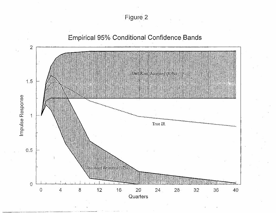
Figure 2

2

1.5

0.5

Empirical 95% Conditional Confidence Bands

00 4 8 12 20 24 28 32

Quarters36 40

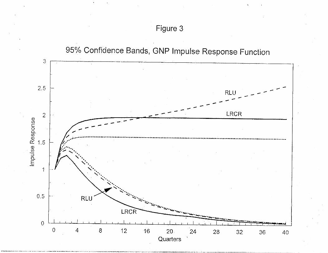
Figure 3

3

95% Confidence Bands, GNP Impulse Response Function

2,5

2

rY 1.5

E

0.5

-- -- " LRCR

RLU

0 4 8 12 16 20Quarters

24 28 36 4O