early stuck pipe detection based on real-time data analysis
TRANSCRIPT

Ahmed Msahli 1 (1) (2) (3) (4) (5) (6) (7) (8) (9) (10) (11) (12) (13) (14) (15) (16) (17) (18) (19)
Msahli Ahmed Master Thesis 2017: supervised by Uni,-Prof.Dipl.-Ing.Dr.mont Gerhard Thonhauser Dipl.-Ing Phillip Wolf-Zo llner Dipl.-Ing Phillip Doppringer
Early Stuck Pipe Detection based on
Real-Time Data Analysis

Ahmed Msahli 2
Affidavit I declare in lieu of oath that I wrote this thesis and performed the associated
research myself using only literature cited in this volume.
Eidesstattliche Erklärung Ich erkläre an Eides statt, dass ich diese Arbeit selbständig verfasst, andere
als die angegebenen Quellen und Hilfsmittel nicht benutzt und mich auch
sonst keiner unerlaubten Hilfsmittel bedient habe.
____________________________________
Name, 27 September 2017

Ahmed Msahli 3
Abstract
This research looks at the work previously done by other scholars regarding pipe sticking
prediction, especially the ones using real-time data, then goes on to prove it possible to
predict impending sticking events using real-time and simulated data.
An algorithm is created based on case based reasoning and improved methods from
previous work. This algorithm is then tested on historical real-time data to come to the
conclusion that it can predict pipe sticking.
This work sheds the light on the potential developments in drilling towards full automation
and better economical practices.

Ahmed Msahli 4
Acknowledgement
I would like to first thank my advisor Univ.-Prof. Dipl.-Ing. Dr.mont. Thonhauser Gerhard of
the University of Leoben for his guidance and help throughout the thesis and to my TDE-
Group advisors Dipl.-Ing Philipp Wolf-Zöllner and Dipl.-Ing Philipp Doppringer for their
assistance, efforts and motivation boosts to allow this thesis to be my own work but to steer
me in the right direction whenever needed.
Last but not least, I would like to thank my family, friends and close ones for being there for
me and supporting me while I was working on this thesis.

Ahmed Msahli 5
Table of Contents
Abstract .................................................................................................................................................. 3
Acknowledgement ............................................................................................................................... 4
List of Figures .......................................................................................................................................... 6
List of Tables ............................................................................................................................................ 7
Introduction ........................................................................................................................................... 8
Literature review .................................................................................................................................. 9
Research Methodology ...................................................................................................................... 17
Findings/Results/Data Analysis ....................................................................................................... 19
Well A: Sticking while drilling ..................................................................................................... 19
Well B: Sticking while POOH ....................................................................................................... 40
Well C: Testing Well (POOH) ....................................................................................................... 47
Well D: Second Testing Well (Drilling) ....................................................................................... 50
Discussion ............................................................................................................................................ 52
Conclusions ......................................................................................................................................... 54
Bibliography ........................................................................................................................................... 55
Appendices .......................................................................................................................................... 57

Ahmed Msahli 6
List of Figures
Figure 1 CBR cycle.................................................................................................................................. 10
Figure 2 Pipe Sticking Radar .................................................................................................................. 12
Figure 3 Method Illustration ................................................................................................................. 15
Figure 4 Well A depth curve .................................................................................................................. 19
Figure 5 Real-Time Hook Load Data - Well A ......................................................................................... 20
Figure 6 Real-Time Standpipe Pressure Data - Well A .......................................................................... 21
Figure 7 Real-Time Surface Torque Data - Well A ................................................................................. 22
Figure 8 Simulated Hook Load Data - Well A......................................................................................... 23
Figure 9 Hook Load Simulated vs R-T ........................................................ Error! Bookmark not defined.
Figure 10 Simulated Standpipe Pressure vs Measured - Well A ........................................................... 24
Figure 11 Simulated Torque Data- Well A ............................................................................................. 25
Figure 12 Simulated Torque vs Measured - Well A ............................................................................... 25
Figure 13 Hook Load Deviation and Rate of Change - Well A ............................................................... 30
Figure 14 Standpipe Pressure Deviation and ROC - Well A ................................................................... 30
Figure 15 Torque Deviation - Well A ..................................................................................................... 31
Figure 16 Torque ROC - Well A .............................................................................................................. 31
Figure 17 Hook Load Deviation and ROC Alerts - Well A ....................................................................... 32
Figure 18 SPP Deviation and ROC Alerts - Well A .................................................................................. 33
Figure 19 Torque Deviation and ROC Alerts - Well A ............................................................................ 33
Figure 20 Sticking Risk Profile #1 - Well A ............................................................................................. 35
Figure 21 Sticking Risk Profile #2 - Well A ............................................................................................. 36
Figure 22 Sticking Risk Profile #3 - Well A ............................................................................................. 36
Figure 23 Hook Load Thresholds ........................................................................................................... 37
Figure 24 SPP Thresholds ...................................................................................................................... 37
Figure 25 Torque Deviation Thresholds ................................................................................................ 38
Figure 26 Torque ROC Thresholds ......................................................................................................... 38
Figure 27 Final Sticking Risk Profile - Well A ......................................................................................... 39
Figure 28 Well B depth curve ................................................................................................................ 40
Figure 29 Hook Load Data Simulated vs R-T - Well B ............................................................................ 41
Figure 30 SPP Simulated vs R-T - Well B ................................................................................................ 41
Figure 31 Torque Simulated vs R-T - Well B .......................................................................................... 42
Figure 32 Hook Load Deviation - Well B ................................................................................................ 43
Figure 33 Hook Load ROC - Well B ........................................................................................................ 43
Figure 34 SPP Deviation - Well B ........................................................................................................... 44
Figure 35 SPP ROC - Well B .................................................................................................................... 44
Figure 36 Torque Deviation - Well B ..................................................................................................... 45
Figure 37 Torque ROC - Well B .............................................................................................................. 45
Figure 38 Sticking Risk Profile - Well B .................................................................................................. 46
Figure 39 Sticking Risk Profile - Well C .................................................................................................. 47
Figure 40 Sticking Risk Profile vs Actual Events - Well C ....................................................................... 48
Figure 41 Sticking Risk Profile vs Actual Even - Well D .......................................................................... 50

Ahmed Msahli 7
List of Tables
Table 1 Inputs and Outputs used for Pipe Sticking Detection ............................................................... 14
Table 2 Friction factors used for simulations ........................................................................................ 22
Table 3 Algorithm Inputs and Outputs .................................................................................................. 26
Table 4 Secong set of Thresholds - Well A ............................................................................................ 35
Table 5 Final Thresholds - Well A .......................................................................................................... 38
Table 6 Thresholds - Well B ................................................................................................................... 45
Table 7 Sticking Events Summary Well C ............................................................................................... 47
Table 8 Head-starts summary - Well C .................................................................................................. 48
Table 9 Sticking Events Summary - Well D ............................................................................................ 51
Table 10 Head-starts summary - Well D ................................................................................................ 51
Table 11 Testing wells Head-starts ........................................................................................................ 52

Ahmed Msahli 8
Introduction
The magnitude of pipe sticking among the problems occurring while drilling is well known
to the oil and gas industry. This problem is costly time wise and economically.
Through the last decades this problem was understood and studied. Best practices were
generated and methods of dealing with it were benchmarked. But despite all that the
problem seem to be persistent and in the weak industry economy that we face today the
issue need to be addressed more.
What was happening alongside that is an accumulation of data. This data is being stored and
not taken advantage of. And if there was an answer for the question posed above, that
answer must be in the data.
The industry is aging and there is so much experience to be let go and put to retirement. For
that the urge to move forward technologically has grown.
A combination of technological advancement and years of experience can crack down the
mountains of data accumulated and is being accumulated day to day. This will eventually
lead to having a strong ground to understanding the data as it is generated in real-time. The
crews will have the time to react, problems such as pipe sticking are going to be avoided and
mitigated and better economy can be eventually achieved.

Ahmed Msahli 9
Literature review
Since the question of pipe sticking has been posed, many approaches have been taken to
tackle the problem. In this literature review the concepts used through the history to deal
with the pipe sticking issue and solve it are addressed and the most recent approaches that
might lead to actual prediction of the phenomenon are analyzed in depth and assessed on
the basis of the added value to this research.
In the early phase, the focus was to understand the pipe sticking physical phenomenon. Most
relevant of these literature are studied in my Bachelor Thesis (Msahli, Pipe Sticking Causes &
Preventions). Physically, total prevention was not possible. After understanding the physical
reasons behind pipe sticking, literature was focused on reducing its occurrence and
generating practices to mitigate it as well as to make freeing the pipe more feasible. Sticking
back then had great impact economically, a study ( Bradley et al. 1991) estimated the yearly
cost of this problem to be $250 million in the late 80s.
The need for pipe sticking prediction was a necessity. The need for it was crucial to reduce
the non-productive time (NPT) which some papers ( such as Muqeem et al. 2012) related 25%
to the sticking. (Joshua Hess 2016) summarized the history of most relevant attempts to
predict pipe sticking. The paper mentioned that since the 80s studies have been conducted in
order to predict the sticking occurrence. It started with statistical analysis to define the
relationships between parameters (Hempkins et al. 1987). Later, more analytical methods
were used with implementation of artificial intelligence tools such as artificial neural
networks (ANN) and support vector machine (SVM). These methods allowed the prediction
of the occurrence of a sticking event during the drilling operation quite accurate, but were
not able to be definitive. Analytical methods lacked the physical aspect.
On the other hand the implementation of the previously mentioned technologies shed the
light on the importance of data in order to understand the phenomenon and solve the
problem as it occurs during drilling. This awareness of the importance of data came
associated with the shift of the industry towards real-time.
For years companies have been accumulating data with less analysis and even more less
applications that would be reflected on the everyday operations.
Recently, many researches targeted the issues above mentioned and many researches have
been performed with the goal of solving drilling problems in real-time while allowing
transfer of experience through automation. This all is seen to be achievable through case
based reasoning (CBR).
The concept of CBR was best introduced in the early 90s by Kolodner, but is still a brand new
concept in the drilling industry. This can be very reflective of the gap the industry has in
technology and in updating methods.

Ahmed Msahli 10
CBR was defined (Kolodner 1992) as follows: “Case-based reasoning means using old
experiences to understand and solve new problems. In case-based reasoning, a reasoned
remembers a previous situation similar to the current one and uses that to solve the new
problem”. The core concept of CBR is simple to understand as it is the basic way humans
learn from experience.
A worth mentioning introduction of CBR in drilling, (Aminul et al. 2008) focused on the
importance of passing the experience attained by the organization and the individuals in it to
those who need it when they do need it. This was described possible through computerized
support for information handling in the purpose of prediction of potential unwanted events
and decision support on a later stage. The first part of this support can be achieved through
this thesis in the case of pipe sticking.
Then, the paper went on to suggest a four steps process to solve CBR problems ( Aamodt
and Plaza 94). The four steps are:
1. Retrieve: collect the similar and relevant cases
2. Reuse: use the knowledge in the retrieved case for solving the problem
3. Revise: revise the proposed solution
4. Retain: retain the experience that can be used in future problem solving
The process is well illustrated in the CBR cycle below.
Figure 1 CBR cycle
The paper managed to put in the scope the key points to solve a drilling problem through
previously available experiences, but failed to provide clear real case use and potential of use
after the planning phase.

Ahmed Msahli 11
Where the previous paper failed, others were successful. After few years, (Dadlier 2013)
presented an automated real-time solution for drilling problems. The solution reduces
drilling risks through applying case-based reasoning to compare the current problem to
historical ones. The main target was to detect and well identify the similar events that came
and somehow led to the event.
The approach is straight forward and presented below.
The solution would consist in the relevant historical cases and related workflows presented
to the operator as soon as there is enough similarity in that case with the current situation.
This is feasible through two forms of machine learning. First, there is pattern recognition
where meaningful pattern are identified and classified into events. Second, display of
historical cases in an order where similarity is measured through attributes and the most
similar one is displayed.
This working principle is similar to what an experienced engineer would do. An experienced
engineer would recall his personal experience or the cases he got exposure to and from there
think of how to react based on what worked or not.
At this point, weather the solution suggested is proven or not, the logic behind it answers the
question of how experience is transmitted from the older generation and their lessons
learned to the younger ones hungrier for experience in an aging industry.
The display is in the radar figure below; where the side notes give recommendations from
best practices and the dashed line represent a 75% matching case, the outer circle is a 50%
case and the center is the current case. The historical case would show up at certain
percentage and direction. This is analogue to submarine radar where the threats are marked
with dots and the closer the higher the risk and where the direction gives away the origin of
the threat.
Hystorical experience
Automation Solution

Ahmed Msahli 12
Figure 2 Pipe Sticking Radar
The paper suggested that the solution can be used for the planning phase as well. An
example of that was the case where it allowed the operator to develop strategies prior to
drilling as well as watching relevant cases in real-time. This is said to have saved $2mo per
incident.
Even in case of success, there are lessons to be learnt. Meaning that, false positives can be
used to improve the platform of the solution.
False positives can be reduced by diving operations. In case they still exist, that leads to the
question of maturing and improving the platform.
Maturing can be tackled straight through analysis of more data and through collaboration
between different involved parties to share experiences and generate protocols.
The suggested solution promises a variety of uses in drilling and surely goes in the direction
of preserving the industry’s knowledge.
After a couple of years, a new approach was published. This approach (Ferreira et al. 2015)
goes in the same direction that the previous one, but focuses on pipe sticking which makes it
more relevant for this thesis and a great encouragement for the chosen direction of research.
In order to deliver a well on plan, the drilling team would need actionable information.

Ahmed Msahli 13
Symptoms of drilling problems needs to be identified prior and delivered in a simple
straight forward way or else the information might just be lost in the huge amount of data
streams and get sent to the data graveyard which is known as data storage.
There are three key elements to make this into a success. They are 24/7 real-time surveillance,
case-based reasoning software and real-time solution to avoid NPT. The solution is provided
when similarities are detected and need expert guidance to achieve less risk and less
operational costs.
This goes as well in the direction of knowledge transfer to machine but do not dismiss the
importance of expert collaboration to provide the final solution.
This is an important half-way step towards Automatisation, with such a solution experts
become able to keep watch over different wells from a remote location and intervene when
their intervention is really needed. This is presented from a management point of view.
Events in this paper were presented as prior symptoms to the actual problem. The software
part will continuously identify the events and help engineers to focus where their focus is
required. It is important to mention that single signal is not enough to mean a problem but it
can be part of a pattern and still requires investigation.
The solution was as well presented as radar with a similar percentage assignment as the
previous paper. This is as well associated with solution protocols and the paper highlights
that it can be done remotely.
This literature presents a logical and effective way to solve the challenges in drilling but
there is a need for practice to prove it working. The scope of it is a bit wide and assesses the
situation from a management point of view, this resulted in a lack of details regarding the
process and the method used to achieve the solution.
In the same direction, another relevant to this thesis approach was taken. The approach
taken by (Kent Salmine et al. , SPE 178888-Ms) consisted of three main steps. First, studying
wells with sticking incidents and gathering a defined type of data, then, patterns detection
and finally alert generation.
Data gathering:
In order to make the solution work on most available rigs and through different types
of operations some contingencies were used on the data selection. Data needs to be
available on most rigs in real-time, informative about the wellbore, fluid and the
drilling string and can be logically related to impending pipe sticking.
This raises already an issue of data consistency between wells, even those drilled by
the same operator. And in this case were only the basic data is used, would it be
enough to be indicative.
The paper suggests that at least one data point per 10 seconds (0.17 Hz) is required.
The data used is divided as follows in the table.
Ahmed Msahli 14
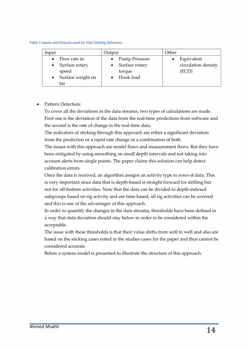
Table 1 Inputs and Outputs used for Pipe Sticking Detection
Input Output Other
Flow rate in
Surface rotary
speed
Surface weight on
bit
Pump Pressure
Surface rotary
torque
Hook load
Equivalent
circulation density
(ECD)
Pattern Detection:
To cover all the deviations in the data streams, two types of calculations are made.
First one is the deviation of the data from the real-time predictions from software and
the second is the rate of change in the real-time data.
The indicators of sticking through this approach are either a significant deviation
from the prediction or a rapid rate change or a combination of both.
The issues with this approach are model flaws and measurement flaws. But they have
been mitigated by using smoothing on small depth intervals and not taking into
account alerts from single points. The paper claims this solution can help detect
calibration errors.
Once the data is received, an algorithm assigns an activity type to rows of data. This
is very important since data that is depth-based is straight forward for drilling but
not for off-bottom activities. Now that the data can be divided to depth-indexed
subgroups based on rig activity and are time-based, all rig activities can be covered
and this is one of the advantages of this approach.
In order to quantify the changes in the data streams, thresholds have been defined in
a way that data deviation should stay below in order to be considered within the
acceptable.
The issue with these thresholds is that their value shifts from well to well and also are
based on the sticking cases noted in the studies cases for the paper and thus cannot be
considered accurate.
Below a system model is presented to illustrate the structure of this approach.

Ahmed Msahli 15
Figure 3 Method Illustration
Deviation from predicted Module:
The deviation can be either positive or negative, depending in the rig activity.
The equation used is as follows
( ) (
)
Rate of change:
If we consider a and b as interval or time or depth, depending on data type.
The rate of change is measured as follows
( ) ( [ ] [ ]
[ ])
[ ] represent the average value of data in the interval y.
Filter:
This block deals with the issues of calibration and measurement errors.
Alert generation:
After defining thresholds and calculating deviation, an alert level can be defined by a
simple division.
This resulted in ranges of alert; [0..1] , ]1..3[ and [3..∞* where the latter would be
limited in the value of three. The reasons behind this specific value are not explained
in the paper, but limiting the values would prevent one factor from dominated the
other alerts.
This resulted in a maximum alert value as following
Where N is the number of parameter used. And in this study, N is equal to three.

Ahmed Msahli 16
So the maximum alert level is 18.
For reasons of practicality and to allow operators an easier guidance through sticking
risks, a concept of “Stuck Pipe Risk” curve was introduced. The curve ranges from 0
to 100% and is drawn simultaneously aside the data streams. The curve is drown
from the following equation
∑
During normal operations while verification, the values were low and said to be
increased as a known risk is approached. For this to be a success, the increase should
be noticed before the event leaving enough time for the crew to react and prevent the
occurrence of the sticking.
Even the paper presented success in real wells, the values were not consistent and the
alert value did not seem representative of the risk magnitude.
This approach was well defined despite of the many assumptions made. There is clear
evidence of the success of it in the practical world, but the success can be limited to a certain
area and lack consistency.
In general, this paper represents a strong logical construction and would contribute greatly
for the guidance of this thesis. The number of assumptions made allows a wide margin for
improvement.

Ahmed Msahli 17
Research Methodology
The goal of this thesis is to prove it possible to predict pipe sticking using real-time
measurement data. Through the studied literature, it was seen that using case based
reasoning aligned with some analysis methods like used in (Ferreira et al. 2015) would allow
reaching this goal.
The process chosen was to develop an algorithm that takes as input the real-time measured
data as well as simulated data and certain related parameters. For this algorithm, two wells
are going to be used for the development phase where the functions are going to be tested
and improved. Those functions are mainly a deviation and rate of change (ROC) functions,
inspired by the work in (Ferreira et al. 2015).
Once the algorithm is developed, it will be tested on two other wells to verify if the final goal
is reached or not. The wells are chosen from a database of wells where sticking occurred. The
choice of the wells is based on the type of operation in play when the event occurred. The
first two are offshore wells where the sticking was in one while drilling and while pulling
out of hole in the other.
The second two are similar.
Besides considering the operation in choosing the wells, the data is later going to be filtered
based on the operation of interest. This will be done using the provided Rig States from
ProNOVA. The rig states would allow easy access to each operation and the time span it
took.
It was possible to filter the data otherwise, but this final product is more accurate and would
allow reaching the goal of this filtering more accurately, which is to avoid having false alerts
from drops or increases in the data streams that are caused by switching from one operation
to the other.
At first, it was planned to filter the data and then use it as input. But doing that would not
allow using the same data parameter for different operation of interest. And because the
operation of interest is inputted in the first deviation function, it is simpler and more efficient
to keep the data intact and just filter the deviation and rate of change after it was calculated
for all. This decision would allow choosing a different operation to monitor without having
to load the data again.
The real-time data chosen for study is the hook load, stand pipe pressure (SPP) and torque.
This data is available in most wells that are equipped for basic real-time measurement. For
the simulation of those streams ProNOVA is used as it provides enough accuracy and
consider alternatives. This is beneficial to choose the right stream in case the friction factor is
not available which the case is in this study.
Literature suggested that the equivalent circulation density (ECD) can be used for better
results. But it defies the purpose of this thesis to use something that might not be available is
some rigs.

Ahmed Msahli 18
The simulated data is simulated using the available information and some guesses or
analogies in some cases. Certain companies, in their policies, do not provide full exposure
regarding the type of equipment, mud or other drilling parameters. For that the simulated
data is plotted against the measured streams and the best fitting one is chosen as an input.
This is very important for the success of this thesis, because getting the wrong simulated
stream could make it impossible to track deviation between simulated and real-time
measured data.
It is important to keep in mind the difference in units between the simulated streams and the
measured ones because those differences change from one company to another. In this case,
there are only powers of ten to be multiplied with and consideration of the different time
indexing.
The first step is to create the basic functions of deviation and rate of change, those functions
included sub-functions that had the calculation point by point done and the operation type
considered. This allowed higher flexibility and much more options in terms of possible
future changes in the method used.
To add more flexibility, a window is added to the functions, where the averaged range in the
ROC can be adjusted by changing this window input as well as allowing the deviation from
simulation function to take average values and not just point by point. This has, as well,
purposes of smoothing the curves and avoiding wrong measurement in bad real-time data
streams.
After calculating the deviations, alerts are generated from these deviations and then those
alerts are added up and used to generate a sticking risk percentage. First, those alerts need
thresholds in order to be generated. The value of deviation is simply divided by the
threshold and that gives an alert.
The literature suggested having thresholds from experience or similar cases but there was no
hint on how to get those values. Thus, the used approach was to try a wide range of values to
attempt limiting the threshold values into smaller ranges. Basically, throwing mud at the
wall to see what sticks. Once a somehow smaller range is defined, it would be much easier to
detect a patter or a logical way of getting the threshold.
In case of success, the second developing well would be used for the purpose of proving the
threshold method right because the third and fourth well should be used with the same
thresholds as the first ones and having those values non-tested would add ambiguity.
For the final sticking risk, the development wells would be matched intentionally with the
historically noted event of the drilled well. As for the testing wells, the risk plots have to be
explainable with those notes associated with the events.
Once the events are matching the obtained curve, the thesis goal in achieved and the
question posed before are answered.

Ahmed Msahli 19
Findings/Results/Data Analysis
At first, two wells where a sticking incident occurred are investigated. The wells were chosen
based on the type of operation and the sticking occurred during.
The first well, we call it well A, the sticking occurred while drilling.
Well A: Sticking while drilling
Well A is an offshore drilled well. The drilling operations in scope are from 350m to 835m of
MD.
The major sticking problem occurred while drilling at 835m and is explained below in
details.
The depth curve of well A is presented below.
Figure 4 Well A depth curve
The first sticking problem in this well appeared at the measured depth of 393m. Erratic
torque was experienced when drilling 36” hole from 390m to 403m at 19:30 July 30, that
resulted in the string becoming stuck at few depth points; 393m , 399m and 402m.
The string was pulled free using an overpull range of 5-25 tons and the reason of this sticking
was reported as possible boulders.
The second sticking incident was reported at a depth of 831m around 20:00 2nd of August
after pulling off bottom, stopping rotation and orienting toolface for sliding.
Packing off was observed and the MWD tool indicated an increase in ECD from 1.13 sg to

Ahmed Msahli 20
1.40 sg which meant that the pack off is above the tool.
Attempts to work the string down were not successful, the increase in torque was not able to
rotate the string and reducing flow to minimize pump off effect and firing the jar down had
no effect.
The team moved the ROV in position to observe the string above the wellhead for any
buckling and reduced the flow with firing the jar but still no go.
While circulating for a while a reduction in string weight was observed which indicated
increased pack off. The pumps were stopped and 19 bars of trapped pressure where
observed.
At this point, overpull was increased gradually with jarring attempts and working the string
upward and downward with some minor progresses at first but then no movements
anymore.
The overpull was increased to max; 346 tons, flow was staged up and pressure increased to
increase push force. The pipe moved 3m before stopping again. After applying these
parameters and working the jar up and down the string was freed.
The increases in hook load and other changes of parameters can be observed below in the
graphs representing the real-time parameters measured for this sticking while drilling event.
These parameters for well A are used to create the base algorithm using their rate of change
and the deviation from the simulated data curves.
Below is found the Real-Time Hook Load data curve.
Figure 5 Real-Time Hook Load Data - Well A
The Hook Load data curve show the shifts and disturbs in the Hook Load before the sticking
happens and at some point the peak would start to represent the added loads in the attempts
of freeing the pipe.

Ahmed Msahli 21
In the first period there is a slight increase of the value which is natural to drilling operation
and addition of stands. Then, the gradual increase till reaching the flat max hook load tells
about the teams approach to resolving the problem.
The second measurement considered is Stand Pipe Pressure which is the total friction
induced pressure loss in the hydraulic circuit. It is measured in real-time for its importance
in mud weight selection.
Below, the real-time measurements of Stand Pipe Pressure are presented.
Figure 6 Real-Time Standpipe Pressure Data - Well A
The increase of the hydraulic circuit and thus the increase of the surface explain the slight
and gradual increase in the value of SPP. Then the drop just happened when the sticking
happened for the simple reason of circulation stopping.
The third measured data used is the Torque data. Knowing the torque is important primarily
to avoid getting stuck and to have better borehole quality and longer equipment lifespan.
The surface torque real time measurement for well A is presented in the figure below.

Ahmed Msahli 22
Figure 7 Real-Time Surface Torque Data - Well A
In order to be able to measure the deviation of real-time data from the predicted range of
values, it is very important to have accurate simulated data streams.
The simulated data streams are provided using ProNova. The inputs needed were BHA
assembly, bit position, casing depths, trajectory and mud rheology properties.
The challenge at this point was that certain information was not available because of non-
disclosure policies for some companies. So in the inputs some numbers were used based on
the closest similar tool size and weight and some approximated through common industry
practices.
In some cases, the range of error was estimated with few tens of kilograms. It is quite
irrelevant in a wellbore.
The simulation then proceeded and the results are presented below.
The first plot below represents the predicted hook load curves during the job performance.
The simulation provided different sets of results; two groups referred to as down and up.
The difference between both is that the hook load when POOH is higher than when RIH for
friction-acting direction. And for each group of results there is five different curves based on
different friction factors that are considered for the simulation.
The friction factors are as follows:
Table 2 Friction factors used for simulations
Friction factors
# #1 #2 #3 #4
0,1 0,2 0,3 0,4 0,5

Ahmed Msahli 23
The numbering in the table is matching to the graph below.
Figure 8 Simulated Hook Load Data - Well A
Among the simulated results one would be used. In the real case that one can be chosen by
determining the properties of the rock or doing a real-time friction analysis. In this case, the
data used would be the one closest in matching most of the Real-time measurement stream.
Matching till the sticking happens is much more important and would be the criteria in
choosing the simulated data for the following steps.
The chosen curve is represented below with the Real-time stream. It is referred to before as
SHLup.
The simulated curve obviously do not account for connections. We can see the R-t value
going to zero when the pipe is in the slips. This might disturb the resulting values of
deviation with the chosen method but that is eliminated since only the drilling time values
would be considered.

Ahmed Msahli 24
Figure 9 Hook Load Simulated vs R-T
The curve above shows how the simulated data follow the real-time trend till the point
where the pipe got stuck and induced higher peaks of hook load where visualized.
The matching quality is great and once the data is filtering based on the operation type then
the results would be more promising.
The second plot is the Stand Pipe Pressure (SPP). It is plotted below versus the real-time
measurement. The two curves match quite accurately in the trend but the simulated values
are higher with a constant value. That is best explained by the fact that the rheology
information was not available and had to be guessed in order to run the simulation.
The shifting value is quite high but the graphs could be matched by simple subtraction of the
extra value. But in this case, the difference would not make any difference in the final results.
Figure 10 Simulated Standpipe Pressure vs Measured - Well A

Ahmed Msahli 25
The time window to investigate is best represented in the graph above.
The graph shows again a pretty accurate prediction regardless of the small shift due to lack
of knowledge in the inputs.
The last plot is for the Torque data. The simulation resulted in five different graphs
associated with the same friction factors as before.
Figure 11 Simulated Torque Data- Well A
These curves are then plotted versus the real-time stream and it shows that the values are too
low to match. This means that the friction factor is higher that is it in the input values. But
that is not the case since the real-time measurement in this well was corrupt for the torque.
Figure 12 Simulated Torque vs Measured - Well A

Ahmed Msahli 26
With the available inputs these curves are accepted but with different considerations when it
comes to the thresholds since that can cover the gap in the deviation between the two
models.
This decision was based on the fact that this well is just for the purpose of creating the first
algorithm used later to test the rest.
Regarding the algorithm, the first step was to determine the inputs and the desired outputs.
Those parameters are listed in the table below.
Table 3 Algorithm Inputs and Outputs
Inputs
Outputs
• Operation time span (tlend, tlstart)
• Types of operations (Opcode)
• Operation in scope ( 330 ; drilling)
• Time index (timeA )
• R-T Measurement data (HLM , MTQ,
SPPM)
• Simulated data (HLS, TQ , SPP)
• Window (10 )
• Threshold boundaries
• Deviation from simulation
• Rate of Change
• Alerts
• Pipe Sticking Risk
Before moving to the structure of the algorithm, some of the inputs are to be explained.
As for the operations, those parameters were already available and can be provided as a
service by TDE in the rig activity report.
In order to save time and be more accurate and efficient those parameters were taken from
the already prepared reports. The operation time span is in two parameters, one that signals
the start and the other the end of the operation associated in the “types of operation” input
referred to as Opcode. The last parameter is the numerical benchmark for operation and is
the number associated with the operation of interest; like in this well drilling (330).
The other inputs are the data as it was detailed above and a window, the window is there to
first allow more flexibility into the averaged intervals. It would have a direct effect on the
rate of change and would allow surpassing measurement errors in deviations. Further effects
of it are presented in the appendix. The last input is are the threshold boundaries and for the
first algorithm the values are set at (+10% , -10%). On a later stage the values would be
adjusted in order to find a logical method of determining better effective values.
Using neural networks to determine the thresholds was brought to the table but then put
away for believing that a more logical and realistic method exists.

Ahmed Msahli 27
The script for deviation and rate of change looks as follows.
HLdev=SDev(tlend,tlstart,Opcode,330,timeA,HLM,HLS,10); HLROC=SROC(tlend,tlstart,Opcode,330,timeA,HLM,10);
The function of specific deviation “Sdev” which outputs the deviation is defined as follow.
function [ SDev ] = SDev( tle,tls,op,opt,time,Rt,sim,R )
SDev=Dev(Rt,sim,R); s=opdet(tle,tls,op,opt,time); k=length(s); for i=1:k if s(i)==0 SDev(i)=0; end end
The first embedded function to explain is “opdet” which would determine the operation
ranges. The function takes as input the operations inputs, all of them, and in addition the
time of operation in scope. Later, the function would assign “1” to the time points where
there is the scope operation in progress and “0” to where other operations are ongoing.
function [ s ] = opdet( tle,tlb,op,opt,time ) ts=Opstarts(tlb,op,opt); te=oprange(tle,op,opt); l=length(ts); k=length(time); s=time*0; for i=1:l for j=1:k if ts(i)<=time(j)&& te(i)>=time(j) s(j)=1; end end end
As shown above in the function SDev first calculates deviation for all time points but then
eliminates the ones where there are different operations than of interest by assigning the
value “0”.
An alternative was into consideration and it consisted of calculating the deviation for where
the “1” value is. This method would have meant less calculation for one example but actually
is more time-consuming for changing operations and testing.

Ahmed Msahli 28
As for how the deviation is calculated, it is presented below in the function “Dev”.
function [ Dev ] = Dev( RT,sim,R ) l=length(RT); Dev=0; for i=1:l s=DevM(i,R,RT,sim); Dev=[Dev;s]; end Dev=Dev(2:l+1);
end
Each value added to the series of Deviation is calculated in the following function “DevM”.
The R value represents the window, where this value is used to determine the mean value
before and after the point is calculation. The effect of R can be reduced or totally removed
but it is as mentioned before important to experiment with the data and check how the
quality affects the results of the foreseen prediction.
function [ DevM ] = DevM(i, R , x , y ) t=i+R; l=i-R; g=length(x); if t>g t=g; end if l<=0 l=i; end x1= mean(x(l:t)); y1= mean(y(l:t)); DevM=((x1-y1)/y1)*100;
end
As for the rate of change, the same approach was applied.
function [ SROC ] = SROC( tle,tls,op,opt,time,Rt,R ) SROC=ROC(Rt,R); s=opdet(tle,tls,op,opt,time); k=length(s); for i=1:k if s(i)==0 SROC(i)=0; end end

Ahmed Msahli 29
The function ROC is the equivalent of function Dev. It takes the results from the next
function ROCM that just calculates the rate of change on each point.
function [ ROC ] = ROC( Rtdata,size ) ROC=0; l=length(Rtdata); for i=1:l s=ROCM(Rtdata,i,size); ROC=[ROC;s]; end ROC=ROC(2:l);
end
This function basically is the same; it just calculates the deviation of the curve within itself.
And in this one the R in needed more to be precise as the results changes directly with the
change of R.
function [ ROCM ] = ROCM( x,i,R ) t=i+R; l=i-R; g=length(x); if t>g t=g; end if l<=0 l=i; end x1= mean(x(l:i)); y1= mean(x(i:t)); ROCM=((y1-x1)/x1)*100;
end
The results for the deviation and rate of change are presented together in the following plot.
The two graphs where of different signs. And for the deviation, the positive thresholds is
irrelevant and the other way around for the rate of change.
There is noted symmetry and the two events show bells shapes of proportional sizes to the
relevance of the sticking event. The increase already puts the light on the significance of the
hook load for the sticking events.

Ahmed Msahli 30
Figure 13 Hook Load Deviation and Rate of Change - Well A
The stand pipe pressure showed a uniform behavior for both deviations with few peeks.
Figure 14 Standpipe Pressure Deviation and ROC - Well A
As for the torque, the Deviation and the rate of change values had far different range of
values that they couldn’t be properly plotted together. The resulting curve for the deviation
has a hyperbolic trend.
The trend might be of significance and requires further investigation, but it is to leave aside
since the actual simulated data do not fit with the measured one.

Ahmed Msahli 31
Figure 15 Torque Deviation - Well A
In the rate of change curve, the values were both positive and negative. It shows that every
stand being drilled had increases and decreases in the torque. And peaks in all of them show
disturbed torque values.
Figure 16 Torque ROC - Well A
After having the rate of change and deviation for data ready, alerts need to be generated.
The alert is the ratio of the change whether it is deviation or ROC to the thresholds that are to
be better defined later.
Since the change curves have both positive and negative values. There needs to be two
thresholds for the sake of have a positive alert and to allow increases and decreases to be
differentiated and weighted differently.

Ahmed Msahli 32
The script part for alerts is as follows.
AlertHLdev=Alert(ThHLdev,NThHLdev,HLdev); AlertHLROC=Alert(ThHLROC,NThHLROC,HLROC);
The Alert function is defined as below. For this function, Alert was given a null value by
being multiplied in the change. This was for the purpose of having the size of the series set in
prior which is recommended on Matlab.
function [ Alert ] = Alert( Th,ThN,change ) l=length(change); Alert=change*0; for i=1:l if change(i)>=0 Alert(i)=change(i)/Th; else Alert(i)=change(i)/ThN; end end end
The resulting alert curves are presented in the following graphs. At this point, there needs to
be a decision on the value of the maximum alert.
It is prior to decide on a value that covers most of the alert points without being too high to
avoid making lower alert levels irrelevant.
The hook load alerts are presented in the following plot.
Figure 17 Hook Load Deviation and ROC Alerts - Well A

Ahmed Msahli 33
The SPP alert shows that only ROC alerts would be of relevance. It is presented in the plot
below.
Figure 18 SPP Deviation and ROC Alerts - Well A
Finally, the torque alerts. Here we can notice that the hyperbolic shape of the deviation
resulted only in one peak, as for the ROC it had three high alert zones which matched with
the peaks in the SPP ROC alert curve.
Figure 19 Torque Deviation and ROC Alerts - Well A
Now that all the alerts are available and the algorithm is tested and working so far. The final
output, the risk of sticking can be calculated.
It is noted that so far the thresholds have not been defined and the values used for the sake
of building the algorithm are +10% and -10%.

Ahmed Msahli 34
The pipe sticking risk look as follows in the script.
It takes as input all the alerts plus the MaxAlert, which is the sum of every maximum alert.
As far, the value of each was 3. This value was presented in the paper (Kent Salmine et al. ,
SPE 178888-Ms) studied in the literature revue and seemed to be efficient.
Below, there is the script of calculating the final risk.
PipeStickingRisk=Risk(MaxAlert,AlertHLdev,AlertSPPdev,AlertHLROC,AlertSPPROC,AlertTQdev,A
lertTQROC);
Below, the risk function is defined. It first limits the alert values to the maximum level and
that is 3.
Then, the sum of the alerts is divided by the maximum alert MaxAlert of the value 18.
function [Risk7 ] = Risk (MaxA,a,b,c,d,e,f) l=length(a); for k=1:l if a(k)>=3 a(k)=3; end end for j=1:l if b(j)>=3 b(j)=3; end end for s=1:l if c(s)>=3 c(s)=3; end end for o=1:l if d(o)>=3 d(o)=3; end end for k=1:l if e(k)>=3 e(k)=3; end end for k=1:l if f(k)>=3 f(k)=3; end end Risk7=100*(a+b+c+d+e+f)/MaxA; end

Ahmed Msahli 35
The pipe sticking risk, when plotted, results in the following plot. At this point, it is
confirmed that the algorithm works and the functions are able to provide the desired
outputs.
The following curve shows two remarkable increases and the latter reaches a higher value.
This suggests that the first one can be associated with the near miss case around 1/8/16 21:33
and the second one with the actual sticking incident.
For that, the first increase should not exceed 50% which is the decided threshold for whether
a sticking is happening or not. The second should be higher that 50% since the sticking is
confirmed.
Anyway, besides adjusting the upper limits the curve needs to be smoothed and adjusted in
a way to avoid misleading peaks. This is to be achieved through adjusting the alert
thresholds.
Figure 20 Sticking Risk Profile #1 - Well A
At this point, the thresholds would be changed and the effects of each change noted in order
to understand and be able to choose the right ones that would provide the conditions
mentioned above.
The first different values of thresholds tested are presented in the table below.
Table 4 Secong set of Thresholds - Well A
Threshold
%
Hook Load SPP Torque
Dev ROC Dev ROC Dev ROC
+ +10 +12 +10 +5 +200 +15
- -12 -12 -12 -20 -10 -20

Ahmed Msahli 36
These values resulted in a smoother curve that is presented below.
The gradual increase in the risk is shown better but the values in all are higher and needs to
be lowered. That can be achieved with higher threshold values.
Figure 21 Sticking Risk Profile #2 - Well A
When higher values are chosen, the result is the following curve. This curve still shows the
wanted increase of risk.
At this point the threshold values used created a range. In order to have the values fitting
with the y-axis line of 50%, the values need to be chosen in those ranges.
Figure 22 Sticking Risk Profile #3 - Well A

Ahmed Msahli 37
With looking back to the deviation and rate of change curves, it was noticed that within the
defined ranges there are deviation values that are the minimum of most peaks. These values
are covered and if they were chosen to be the thresholds only the extra deviation would be
accounted for and then deviations would be accounted for more efficiently.
Those values are taken from each deviation or rate of change and are run through the
algorithm.
Below, those threshold values are shown in the respective plots.
Figure 23 Hook Load Thresholds
Figure 24 SPP Thresholds

Ahmed Msahli 38
Figure 25 Torque Deviation Thresholds
Figure 26 Torque ROC Thresholds
The new threshold values are summarized in the table below.
Table 5 Final Thresholds - Well A
Threshold
%
Hook Load SPP Torque
Dev ROC Dev ROC Dev ROC
+ +3 +8 +25 +3 +10k +15
- -18 -12 -27 -2 -10 -20

Ahmed Msahli 39
As those values ran through the algorithm, the sticking risk was as follows in the plot.
Those values are more acceptable than any result before and it was logical to pick values
where only the remarkable peaks are effective. The risk profile is accepted and the threshold
choosing method is standing until being proven accurate through the next well.
Figure 27 Final Sticking Risk Profile - Well A
The curve above shows a very early alert for the final sticking as it gives a 02:05h head-start.
The value seems too good to be real especially compared to the value presented in the
related studied literature. But it is explainable, since the curve was fitted to the purpose.

Ahmed Msahli 40
Well B: Sticking while POOH
The second well, well B, has an occurring of sticking while pulling out of hole. The sticking
occurred after the target depth was reached.
Around 5th May 2016 17h, with a measured depth of 5201 m, the pipe was stuck at 2348 m
while tripping out. The crew attempted to free the pipe through the following sequence:
Get rotation with torque up to 55 kNm and to run in hole with jarring downward but
with no go.
Jarred downwards 10 times, applied 60 kNm torque and attempted again.
Jarred up 5 times and pulled with 345 ton.
Jarred 5 times down with no torque.
Jarred up 5 times and pulled with 345 ton.
Continued jarring up and down with torque only when jarring down.
Performed slip and cut then drop check.
Continued jarring up and down in sequences.
Maintenance.
Waited on wireline cutting equipment.
Installed slips with 215 ton tension.
Cutting toolstring and correlating.
POOH to 275 m.
The process can be seen in the graph below through the bit position in time and depth.
Figure 28 Well B depth curve

Ahmed Msahli 41
Similar to well A, the data for well B was plotted real-time vs. simulations and the best fitting
curve was chosen to be used in the algorithm.
In the plot below, it is seen that HLUP follows the measured curve till the sticking happens
and thus it was chosen.
Figure 29 Hook Load Data Simulated vs R-T - Well B
The standpipe pressure is acceptable, but differs from well A where there was just a value
too be added. Here, the curves cross two times where one is just before the sticking occurred.
That might result in a strong indication.
Figure 30 SPP Simulated vs R-T - Well B

Ahmed Msahli 42
The last curve of the input data below show the torque simulated curves matching the real-
time curve with slight deviations before the occurring of the sticking.
Figure 31 Torque Simulated vs R-T - Well B
The curves so far promise good indications to before the sticking event happens. This can be
proven through running it through the algorithm and picking the right thresholds.
Only few inputs are to be changed in order to adapt the old algorithm to this well. Mainly
those are the type of operation in scope and the indexing of the inputs.
Once the algorithm filters out all operations other than the POOH, only small data points are
left. This would make reading the curves much more challenging.
Below, the deviation curves for HL, SPP and Torque are presented.
The thresholds are going to be picked at this point in order to test and to prove working the
method of choosing them that has been noticed through the first well.
In case those thresholds provide a sound alert in this well, this method is then decided to be
the way to go for thresholds.

Ahmed Msahli 43
Figure 32 Hook Load Deviation - Well B
Figure 33 Hook Load ROC - Well B

Ahmed Msahli 44
Figure 34 SPP Deviation - Well B
Figure 35 SPP ROC - Well B

Ahmed Msahli 45
Figure 36 Torque Deviation - Well B
Figure 37 Torque ROC - Well B
The thresholds deducted visually are summarized in the table below.
Those thresholds are not precise but they would be enough to tell if there would be a decent
alert signaling the sticking before it occurs.
Table 6 Thresholds - Well B
Threshold
%
Hook Load SPP Torque
Dev ROC Dev ROC Dev ROC
+ +10 +4000 +10 +10 +30 +1000
- -40 -1000 -40 -10 -50 -10

Ahmed Msahli 46
After running the entire algorithm, the result is presented in the plot below.
Figure 38 Sticking Risk Profile - Well B
It can be seen that there is a significant alert that precedes the sticking event with 12:30h. The
thresholds chosen were efficient and this is enough to prove the logic behind choosing those
thresholds adds up.
At this point, those two wells provide alerts with good head-starts. The algorithm is now
going to be tested on two well, well C and Well D. The purpose of this testing is to see if the
algorithm is enough to provide an alert in similar cases.
Well C has a sticking occurring while POOH while the sticking in well D occurs while
drilling. In order for the goal of this thesis to be met, the thresholds are going to be kept the
same and nothing would change besides the inputted data.

Ahmed Msahli 47
Well C: Testing Well (POOH)
The third well was run through the algorithm with the same parameters and thresholds as
well B since the sticking is while POOH.
The output is presented in the plot below.
Figure 39 Sticking Risk Profile - Well C
Not all peaks exceed 50%. A first look to the plot cannot tell whether it worked or not.
The events in this plot need to be checked against the actual record of event in order to
determine how successful this method in predicting the sticking event.
The sticking events that have occurred in reality are summarized in the table below.
Table 7 Sticking Events Summary Well C
Event # Time of
Occurrence
Description
Event 1 Dec-2 16:00 Experienced stuck pipe when pulling string up at the
depth of 1105m MD. Established circulation and rotation
and were able to work string free.
Event 2 Dec-5 23:15 Torque increased and pack-off was observed. Pressure
increased before pumps were shut down.
30 bars were trapped in DP after pack-off. String stuck
with hole at 2497m MD.
String worked free and pressure in DP dropped off.
Event 3 Dec-7 01:15 Increase in torque and pack-off at 1569m (hole MD
2497m). Shut down pumps. String stuck and a hook load
of 225 ton is experienced because of rig heave.
Worked string free and circulated.

Ahmed Msahli 48
Event 4 Dec-7 16:15 String got stuck while attempting POOH. Worked pipe
up and down with attempts to establish circulation
without success. With max overpull, string was free to
rotate.
While working string, torque gradually increased.
Attempted jarring up and down with no success.
Concluded that hole packed off above the jar.
Increased torque, pipe rotation and gradually pressured
up string. Observed decrease in torque and pressure with
return in trip tank. Circulated and then continued POOH.
The event summerized in the table can be matched with the pipe sticking risk plot. This is
displayed in the plot below.
Figure 40 Sticking Risk Profile vs Actual Events - Well C
It is observed that for each sticking event there is a risk exceeding 50% except for the first
event where the value was a little bit below.
The first event was less relevant compared to the next three events. The second event was
signaled with a very strong risk percentage while the third and fourth had a consistently
increasing strong signal. Those signals are enough to tip the crew with the sticking through
the following head-starts in the table below.
Table 8 Head-starts summary - Well C
Event # Head-start (h)
Event 1 06:56
Event 2 05:10
Event 3 & 4 07:30
E1 E2 E3
E4

Ahmed Msahli 49
Among the peaks that exceeded the 50% line, there were two single peaks. Those peaks are
different from the other risk indicators, for being a single point and far from any other
points.
These two points can be seen as measurement errors and can be put aside.

Ahmed Msahli 50
Well D: Second Testing Well (Drilling)
For the second testing well, well D, the sticking events occurred while drilling. The data from
well D is used with the same parameters and threshold values of well A except for the
Torque thresholds. Those thresholds had to be adjusted since the values in well A were
based on badly-fitting simulation because of the lack in simulation inputs.
The difference is that in well A, the torque contribution to the overall sticking risk was
reduced while in this well the contribution is reasonably based on the threshold choosing
method.
The plot below represents the outputted plot from running well D through the same
algorithm on well A. Signaled in red are the sticking events.
Figure 41 Sticking Risk Profile vs Actual Even - Well D
The plot above shows three sticking events. Those events show an increase similar to the
ones in well A.
Those events match with the recorded history of the well. It is summarized in the table
below.
E1 E3
E2

Ahmed Msahli 51
Table 9 Sticking Events Summary - Well D
Event # Time of
Occurrence
Description
Event 1 Dec-22 11:29 Stuck pipe observed while pulling up for connection
while drilling a 12 ¼ “ hole from 2944.5 m to 2961 m
MD.
Attempted to rotate but without success. Jarred string
several times, moving around 1m each time.
Increased flow and attempted to rotate, without
success.
Reduced flow and jarred string free.
Event 2 Dec-22 15:25 Pipe got stuck after connection while drilling from
2961 m to 2980 m. The string came free with 36 kNm
and 800 lpm.
Event 3 Dec-22 22:10 Well static after flow check for 10 mins. Observed
overpull when pulling out of hole and string was
stuck at MD of 3038.
Established circulation in steps and pulled the pipe
free.
The sticking events match with the plot perfectly. Testing this well is successful and provides
the following head-starts for the events.
Table 10 Head-starts summary - Well D
Event # Head-start
Event 1 01:15
Event 2 01:23
Event 3 03:28

Ahmed Msahli 52
Discussion
In order to reach the desired result from this thesis, the testing wells needed to provide a
head-start to the right events where sticking occurred. The head-starts were noted and are
actually enough for the crew to react and avoid or mitigate the sticking if this was tested in
reality.
In the literature, head-starts were ranging between 48mins and few hours. So far, the values
recorded are much better. This can be due to the difference in the wells nature as the wells in
literature are mainly drilled in shale plays and the ones used in this thesis are North Sea
offshore wells. Other possible reason is the difference in data like better quality of
measurements in real-time or that the simulated data provided by ProNOVA is more
accurate than the simulations used.
The results of the two testing wells are summarized in the table below.
Table 11 Testing wells Head-starts
Well C-POOH Well D-Drilling
Event # Head-start (h) Event # Head-start
Event 1 06:56 Event 1 01:15
Event 2 05:10 Event 2 01:23
Event 3 & 4 07:30 Event 3 03:28
It was noticed while creating the algorithm through wells A and B that well B had a much
higher head-start given; 12:30h compared to 02:05h for well A. This was seen at first as single
case. But now that the results of the two testing wells are compared, this seems like a pattern.
This method gives much earlier alerts when the sticking is occurring while POOH.
In the process of creating the algorithm, some details were taken from the mentioned
literature but the core functions and the reasoning was adapted to the type of data provided.
It was very helpful to have the operations provided aside for each well. Such information
would allow better use of the real-time data.
An important issue was the finding of thresholds. Literature only described the role these
thresholds and what they might look like to have a feeling for them. But there were no
indication on how to get them.
The method developed in this thesis was logical since knowing the needed outcome would
allow fixing a range for the threshold and the smaller range gave out the values much easier.
Those values did work greatly and count as successful thresholds but they are taken
graphically and lack accuracy.
Improving them is believed to improve the head-starts for the while-drilling sticking events.
There might not be a significant difference after all once both scenarios are optimized.

Ahmed Msahli 53
In the sticking risk plots of the two wells, there have been single peaks that exceeded the 50%
value. Those peaks are single points and were neglected in the process. But this raises the
issue of whether using a window to average the data points before using was enough to
surpass the bad measurement points.
The result of this method is very data quality dependent and this sheds more light on the
importance of obtaining good data in the industry and the issues of data management in the
future of drilling.

Ahmed Msahli 54
Conclusions
This thesis has proven it possible to predict impending pipe sticking in the main two drilling
operations that sticking occurs through. The objective was to create an algorithm that takes
as input the real-time data and a simulated data and used them to give an alert prior to any
sticking event regardless to the reason or type of sticking.
At this end, the objective has been reached successfully.
This result depended on many factors such as the quality of the measured data and the
accuracy of the simulated streams in matching the measured ones. This issue is wider in the
oil and gas industry as there is accumulation of great amounts of data while there is less
interest in interpreting the data and making more value of it that just stored bits.
This used approach is considered simple and straight forward. There is definitely more that
can be withdrawn from the data to put the industry ahead of classical problems such as pipe
sticking.
The calculated deviation and rate of change can be used as primary information and there is
a huge potential of what can be deducted and used as indicators. Also, there is potential to
use more trend analysis and experiment with data channels to reach more advanced and
useful results such as differentiating between types of sticking.
In short, there is great potential for next steps in this study but the road is long to go until the
full use of the real-time data is achieved and the knowledge is passed from human experts to
machine as KPIs.

Ahmed Msahli 55
Bibliography 1. Improved Efficiency & knowledge Based Support of Oil Well Drilling through Cased Based
Reasoning (CBR) Approach. Aminul M. Islam and Pal Shalle, Norwegian University of Science &
Technology , Trondheim. Amsterdam, The Netherlands : Society of Petroleum Engineers, 2008. SPE-
111849-MS.
2. Automated Decision Support to Enhance While-Drilling Decision Making: Where Does it fit Whithin
Drilling Automation? Andreas Sadlier, Baker Hughes, Ian Says , Baker Hughes, and Ryan Hanson,
Verdande Technology. Amsterdam , The Netherlands : SPE/IADC, 2013. SPE/IADC 163430.
3. Developing Industrial Case-Based Reasoning Applications Using the INRECA Methodology. Ralph
Bergmann, Mehmet Göker. 1999.
4. An Introduction to Case-Based Reasoning. Kolodner, Janet L. Atlanta, USA : s.n., 1992, Bd. Artificial
Intelligence Review 6.
5. On the Role of Abstraction in Case-Based Reasoning. Ralph Bergmann, Wolfgang Wike.
Kaiserslautern, Germany : University of Kaiserslautern.
6. Application of Case-Based Reasoning for Well Fracturing Planning and Execution. Andrei Popa,
SPE, William Wood, SPE, Steve Cassidy, SPE Chevron North America Exploration and Production.
Alaska , USA : SPE, 2011. SPE 144471.
7. Stuck Pipe Prediction Using Automated Reat-Time Modeling and Data Analysis. Kent Salminen,
Curtis Cheatham, Mark Smith, and Khaydar Valiulin, Weatherford. Texas, USA : s.n., 2016. SPE-
178888-MS.
8. Pipe Sticking Prediction Using LWD Real-Time Measurments. Joshua Hess, Baker Hughes Inc.
Texas, USA : s.n., 2016. SPE-178828-MS.
9. Stuck-Pipe Prediction With Automated Real-Time Modeling and Data Analysis. JPT. s.l. : JPT, 2016.
SPE-0616-0072-JPT.
10. Automated Decision Support and Expert Collaboration Avoid Stuck Pipe and Improve Drilling
Operations in Offshore Brazil Subsalt Well. Ana Paula L. A. Ferreira, Daltro J. L. Cavalha, and Rogerio
M. Rodrigues, Petrobras S. A und David M. Schnell, Ian J. Thonson, Rafael C. Babtista, and Sandro
B. Alves, Baker Hughes Inc. Texas, USA : Offshore Technology Conference, 2015. OTC-25838-MS.
11. Quantifying Stuck Pipe Risk in Gulf of Mexico Oil and Gas Drilling. A.P. Wisnie, Conoco Inc, and
Zhiwel Zhu, U. of Southwestern Louisiana. New Orleans , USA : s.n., 1994. SPE-28298-MS.
12. Realtime Monitoring, Using All Available Data, Plays A Vital Role In Successful Drilling Operations.
Cory Moore, Eamonn Doyle, Karol Jewula, Lukasz Karda, Tim Sheehy, and Stephen O'Connor, Ikon
Science , Obren Djordjevic, Murphy Exploration & Production Company. Texas, USA : s.n., 2016.
OTC-27145-MS.
13. Realtime Drilling Geomechanics Service, Case Study, Offshore Malaysia. Babak Heidari and Sook
Ting Leong, Schlunberger und Nguyen Truong Son and M Zafril B Aznor, Petronas, Carigali Sdn. Bhd.

Ahmed Msahli 56
Muscat, Oman : s.n., 2015. SPE-172977-MS.
14. A Practical Method To Minimize Stuck Pipe Integrating Surface and MWD Measurements. J.P.
Belaskle, D.P. McCann, and J.F. Leshikar, Anadrill/Schlumberger. Dallas , Texas, USA : s.n., 1994.
SPE-27494-MS.
15. Tracking Stuck Pipe Probability While Drilling. J.A. Howard, Enertech Engineering & Research Co.
and S.B. Glover, Tnertech Europe. Dallas, Texas, USA : s.n., 1994. SPE-27528-MS.
16. Advances in Prediction of Stuck Pipe Using Multivariate Statistical Analysis. M.W. Biegler, Exxom
Production Research Co., and G.R. Kuhn, Exxon Co. USA. Dallas, Texas, USA : s.n., 1994. SPE-27529-
MS.
17. Stuck-Pipe Prevention Solutions in Deep Gas Drilling; New Approaches. Julio M. Guzman and
Mohamed E. Khalil, SPE, Saudi Aramco und and Nicolas Orban, Mohammed Ahmed Mohiuddin,
Jaywant Verma, and Sukesh Ganda, SPE, Schlumberger. Al-Khobar, Saudi Arabia : s.n., 2012. SPE-
160875-MS.
18. Solution of Common Stuck Pipe Problems Through the Adaptation of Torque Drag Calculations.
G.A. Haduch, DRD Corp., and R.L. Procter and D.A. Samuels, Shell U.K. E&P. Dallas, Texas, USA : s.n.,
1994. SPE-27490-MS.
19. Torque and Drag in Directional Wells-Prediction and Measurement. C.A. Johancsik, D.B. Friesen,
Rapier Dawson, SPE, Exxon Production Research Co. s.l. : JPT. SPE-11380-PA.
20. New Approach to Differential Sticking. Courteille, J.M. and Zurdo, C.A. SPE Annual Technical
Conference and Exhibition, Las Vegas Nevada : SPE, 1985. 14244.
21. Quantifying Stuck Pipe Risk in Gulf of Mexico Oil and Gas Drilling. A.P. Wisnie, Conoco Inc, and
Zheiwei Zhu. SPE, s.l. : University Of Southwestern Louisiana. 28298.

Ahmed Msahli 57
Appendices

Ahmed Msahli 58

Ahmed Msahli 59