Early-Time Stability of Decelerating Shocks

F. W. Doss and R. P. DrakeDepartment of Atmospheric, Oceanic, and Space Sciences, University of Michigan, Ann Arbor, MI 48105

H. F. RobeyLawrence Livermore National Laboratory, Livermore, California 94550

ABSTRACT

We consider the decelerating shock instability of Vishniac for a finite layer of constant den-sity. This serves both to clarify which aspects of the Vishniac instability mechanism depend oncompressible effects away from the shock front and also to incorporate additional effects of finitelayer thickness. This work has implications for experiments attempting to reproduce the essen-tial physics of astrophysical shocks, in particular their minimum necessary lateral dimensions tocontain all the relevant dynamics.

Subject headings: hydrodynamics – instabilities – shock waves

1. Introduction

Vishniac (1983) outlined a theory of instabili-ties for a system of a decelerating shock accret-ing mass, modeled as a thin mass shell layer pos-sessing no internal structure. In Vishniac andRyu (1989), the theory was expanded to include alayer of post-shock material, exponentially attenu-ating in density. Other work (Bertschinger (1986);Kushnir et al. (2005); among others) has describedthe perturbation of self-similar solutions for thepost-shock flow. The present work complementsthese investigations, modeling the post-shock flowas a finite thickness layer of constant density andconsidering both compressible and incompressiblepost-shock states. This allows us both to moreclearly understand which mechanisms depend onthe compressibility of the shocked gas and whichare common to any shock system undergoing de-celeration.

Early in the lifetime of an impulsively drivenshock, when the post-shock layer thickness is smallcompared to its compressible length scale, an ex-ponential scale cannot be formed and the densityprofile may be closely approximated by a squarewave, as a fluid everywhere of constant density. Inthe shock’s frame, upstream fluid is entering the

shock with a speed Vs and exiting it with a speedU = Vsη, where η is the inverse compression ra-tio associated with the shock, including both theviscous density increase and any subsequent, lo-calized further density increase in consequence ofradiative cooling (Drake 2006).

We have also in mind throughout this paperexperiments (Reighard et al. 2006; Bouquet et al.2004; Bozier et al. 1986) that have been carried outto investigate radiating shock dynamics. Experi-ments of this type are often designed to be scaledto relevant astrophysical investigation (Reming-ton et al. 2006). The particular experiments ofReighard et al. (2006) feature characteristic shockvelocities of over 100 km/sec, shock tubes with 625µm diameters, and strong deceleration throughoutthe shocks’ lifetimes.

2. System of a Decelerating Shock with aDense Downstream Layer

We consider the shock in its own, deceleratingframe. The system is depicted in Figure 1. Theshock is placed at z = 0, with flow entering itfrom the negative z direction at speed Vs, densityρ0, and with negligible thermal pressure. Flow isexiting the shock toward positive z with speed U ,

1

arX

iv:0

906.

1222

v3 [

astr

o-ph

.SR

] 9

Sep

201

0

unperturbed system perturbed system

δz

wu

z = H

z = 0

Pi

Vs-

ρ0, Vs

ρ, U

dense rear layer

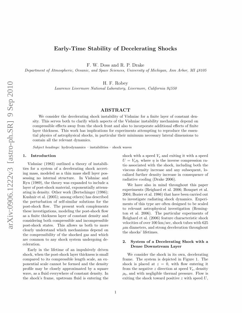
Fig. 1.— Schematic of the decelerating shock sys-tem. The solid black line is the shock, the dashedline above the dense rear layer is the rear mate-rial interface. The left-hand arrow depicts the in-frame inertial force with acceleration (−Vs).

density ρ, and isotropic pressure P . We will modelthe downstream, rear layer as a constant densityregion of finite, increasing thickness from z = 0 toz = H. The rear surface of the dense layer will betaken to be a free interface at constant pressure.Beyond the rear layer will be taken as a region ofconstant thermal pressure Pi.

The native surface wave modes in the systemwill be right- and left-propagating waves on thetwo surfaces of the dense layer, leading to fourmodes in total. As drawn in Figure 1, the up-per surface, a material discontinuity, is stable ifthe shock frame is decelerating and is character-ized by surface gravity modes. The bottom sur-face, a shock at which compressibility is not sup-pressed, will feature propagating acoustic modes.The waves which appear in our coupled systemwill be modifications of these waves which appearon these surfaces in isolation. In particular, themodified acoustic waves along the shock surfacewill be identified as bending modes of the entiredense layer.

In order to understand the fundamental causeof the instability, we will here be consideringthe fluid both ahead and behind the shock tobe held at (different) densities constant in bothspace and time. This practice is described anddefended by Hayes and Probstein (1966), who intheir book “consider constant-density hypersonicflows, though we should never consider the fluidin a hypersonic flow as incompressible.” Thepressure profile behind the shock is hydrostatic,

P (z) = Pi− (H − z)ρVs, which leads to increasingpressure at the shock front when the shock is de-celerating. Perturbations to density by the wavesunder investigation will be discussed.

3. Linear Perturbations of the System

3.1. Solutions Inside the Post-Shock Fluid

We begin with the inviscid fluid equations

ρ(∂tv + v · ∇v) = −∇P − ρVsz (1)

∂tρ+ v · ∇ρ = −ρ∇ · v (2)

with total velocity v = (u, 0, w + U) and P =P + δP . We will insert the perturbation δρ onlyin the continuity equation; the coupling of δρ tothe frame’s acceleration will be suppressed. Thisallows us to ignore mode purely internal to thelayer, concentrating on the overall shock and layersystem. Since log ρ/ρ0 >> log (ρ+ δρ)/ρ for anyreasonable density perturbations, we expect thedynamics of the system to be dominated by thecompression at the shock. The omission of theterm δρVs is also required for consistency with theassumption of our square wave density profile; thesystem will otherwise begin to evolve into an ex-ponential atmosphere.

We first let the perturbations u,w, δP havetime and space dependence as ent+ikx, with k realand n complex. We then linearize the x- and z-components of the momentum equation to obtain

(n+ U∂z)u = − ikδPρ

(3)

(n+ U∂z)w + w∂zU = −∂zδPρ

. (4)

We expressed the perturbed continuity equationin terms of perturbed pressure,

iku+ ∂zw = − (n+ U∂z)δρ

ρ= − (n+ U∂z)δP

ρc2s(5)

where c2s = ∂P/∂ρ. We solve Equation 3 for δPusing Equation 5, and discard terms of order U/csto obtain

δP =ρ

k2 + n2/c2s(n+ U∂z)(−∂zw) (6)

and insert that into Equation 4 to obtain a new

2

equation for z-momentum:

(n+U∂z)w+w∂zU = ∂z

(1

k2 + n2/c2s(n+ U∂z)(∂zw)

)(7)

which can now be written as a differential equationfor w (taking U and cs constant throughout thepost-shock layer),(

U

k2 + n2/c2s∂3z +

n

k2 + n2/c2s∂2z − U∂z − n

)w = 0.

(8)For a treatment of the problem where cs variesthrough the layer, see Appendix A.

We define

j =√k2 + n2/c2s, (9)

which describes the effective lateral wavenumber.As a wave approaches the acoustic case, n2 =−k2c2s, the wave becomes purely longitudinal andj tends toward zero. Equation 8 has the generalsolution

w = Aejz +Be−jz + Ce−nz/U . (10)

The system accordingly has three boundary con-ditions at its two interfaces: the shock and therear surface. We note that the shock frame’s ac-celeration Vs does not appear in the general formof the perturbations; it will enter into the systemthrough the boundary conditions.

The last term in Equation 10 is a consequenceof the background flow U and is closely connectedwith structures convecting downstream with thatvelocity. It is instructive to consider the generalsolution for w in the frame of the rear surface.We introduce the coordinate z′ = Ut − z. In ad-dition, we will now write explicitly the implicittime-dependence ent. The general solution is w =Ae(n+jU)t−jz′+nt + Be(n−jU)t+jz′ + Cenz

′/U . Wesee that the third term has no time-dependence inthe frame of the rear layer. In the frame of therear surface, these flow structures are generatedby perturbations in the shock surface as the shockpasses some point in space, and do not evolve fur-ther. Therefore, in the frame of the shock, thisterm describes flow structures convecting down-stream through the flow with constant velocity U .We take the shock to have been perfectly planar atthe instant, some time past, at which the shock’sdeceleration and rear layer formation began. This

allows us to explicitly set C = 0 at the rear layer.We assume however that the perturbation begansufficiently early in time that our treatment usingFourier modes is sufficient, so no further informa-tion from initial conditions will be incorporated atthis time.

3.2. Infinitely Thin Layer

We recall that the dispersion relation for thethin shell instability in its most simple form, with-out the effects of compression, is in Vishniac andRyu (1989) written in the form

n4 + n2c2sk2 − k2VsPi

σ= 0 (11)

where σ is the areal mass density of the (infinitely)thin layer, and all other variables are as we havedefined them. Early work (Vishniac 1983) derivedthis expression for a shock of infinitesimal heightbut finite areal density. Such a shock, maintainingan infinitely thin layer height while continuing toaccrete mass from the incoming flow, would in ouranalysis be described as the limit of an infinitecompression, η → 0. We should expect solutionswe obtain for layers of finite thickness to approachEquation 11 in this limit.

3.3. Free Rear Surface

We construct the boundary condition describ-ing a free layer at z = H by applying δP =ρ(−Vs)δz at z = H, with ∂tδz = w. Using Equa-tion 10 and our earlier expression for δP , Equation6, the boundary condition becomes

A(n2 − jVs)ejH +B(−n2 − jVs)e−jH = 0 (12)

where C has been explicitly set to zero as discussedabove. Equation 12 is a boundary condition wellknown to generate surface gravity waves, when j =k and when paired with a rigid boundary conditionat z = 0.

At the shock surface, we must perturb the shockmomentum jump condition in the frame of themoving shock. The perturbed shock surface mov-ing upward in Figure 1 sees a weaker incomingflow. In addition, by raising the shock surface inthe hydrostatic pressure field, the effective post-shock pressure drops by an amount Vsρδz. Ourjump condition has now become

ρ0(Vs − w)2 = ρU2 + (P + Vsρδz + δP ), (13a)

3

from which we obtain a boundary condition (us-ing ρ0Vs = ρU , δz = w/n(1 − η), and our earlierexpression for δP in Equation 6)(

U

j2∂2z +

n

j2∂z −

(Vs

n(1− η)+ 2U

))w

∣∣∣∣∣z=0

= 0.

(13b)The expression for ∂tδz comes from conservation

of mass across the shock. With density pertur-bations suppressed, as discussed above, we have abalance of mass flux with ρ0Vs entering and ρU+wleaving the shock, with the shock moving at speed∂tδz.

η =U

Vs=U + w − ∂tδzVs − ∂tδz

(14a)

implying (with ∂t = n)

w∣∣∣z=0

= (1− η)nδz (14b)

The third boundary condition comes fromoblique shock relations. Letting β be the an-gle of the shock surface perturbation, continu-ity of the tangential flow requires to first orderu ≈ Vsβ = (ik)Vsδz. Applying the continuityequation of Equation 5 just downstream of theshock, and applying Equations 6 and 14b(

∂z −Vsk

2

n(1− η)

)w

∣∣∣∣z=0

= − (n+ U∂z)δP

ρc2s(15a)

which evaluates to(∂z −

Vsj2

n(1− η)

)w

∣∣∣∣z=0

= 0 (15b)

Simultaneously applying these three conditions(equations 12, 13b, and 15b) on w, one demandsfor nonzero solutions that the determinant of thematrix of coefficients of A, B, and C, shown col-lected in Equation 16, must be zero,∣∣∣∣∣∣∣

(n2 − jVs)ejH (−n2 − jVs)e−jH 0

−nj + U + Vs

n(1−η)nj + U + Vs

n(1−η) 2U + Vs

n(1−η)1j −

Vs

n(1−η) − 1j −

Vs

n(1−η) − nUj2 −

Vs

n(1−η)

∣∣∣∣∣∣∣ = 0

(16)

From this one obtains, with some manipulation,the dispersion relation,

0 = (1− η)n2 + j2UVs + (jVs + 2njU)×((n3 + j2UVs)− (njVs + n2jU) tanh jH

(n3 + j2UVs) tanh jH − (njVs + n2jU)

).

(17)

We will take, as in Vishniac and Ryu (1989), theproduct UVs to be equivalent to an average soundspeed squared 〈c2s〉, which we shall not henceforthdistinguish from the sound speed c2s of materialcompressibility. The qualitative classification ofsolutions to Equation 17 depends strongly on thelayer thickness H, specifically on its relation to thecompressible scale height UVs/|Vs| = c2s/|Vs|. Weshall explore this dependence in what follows.

We will now investigate the range in whichwavelengths of perturbations are not much shorterthan H, and will approximate tanh jH ≈ jH.The existence of the critical H is easiest to see inthe limit of very strong, highly compressive shocks(U → 0 while Vs →∞ in such a way that UVs = c2sand Vs remain constant). By expanding j, we maywrite the dispersion relation as,

Tn4 + n2

(k2c2s −

V 2s

c2sSZ

)− k2V 2

s S = 0 (18a)

where we have introduced scale factors

T = 2− η (18b)

S = 1 +c2s/VsH

(18c)

Z = 1− η(S − 1)

S. (18d)

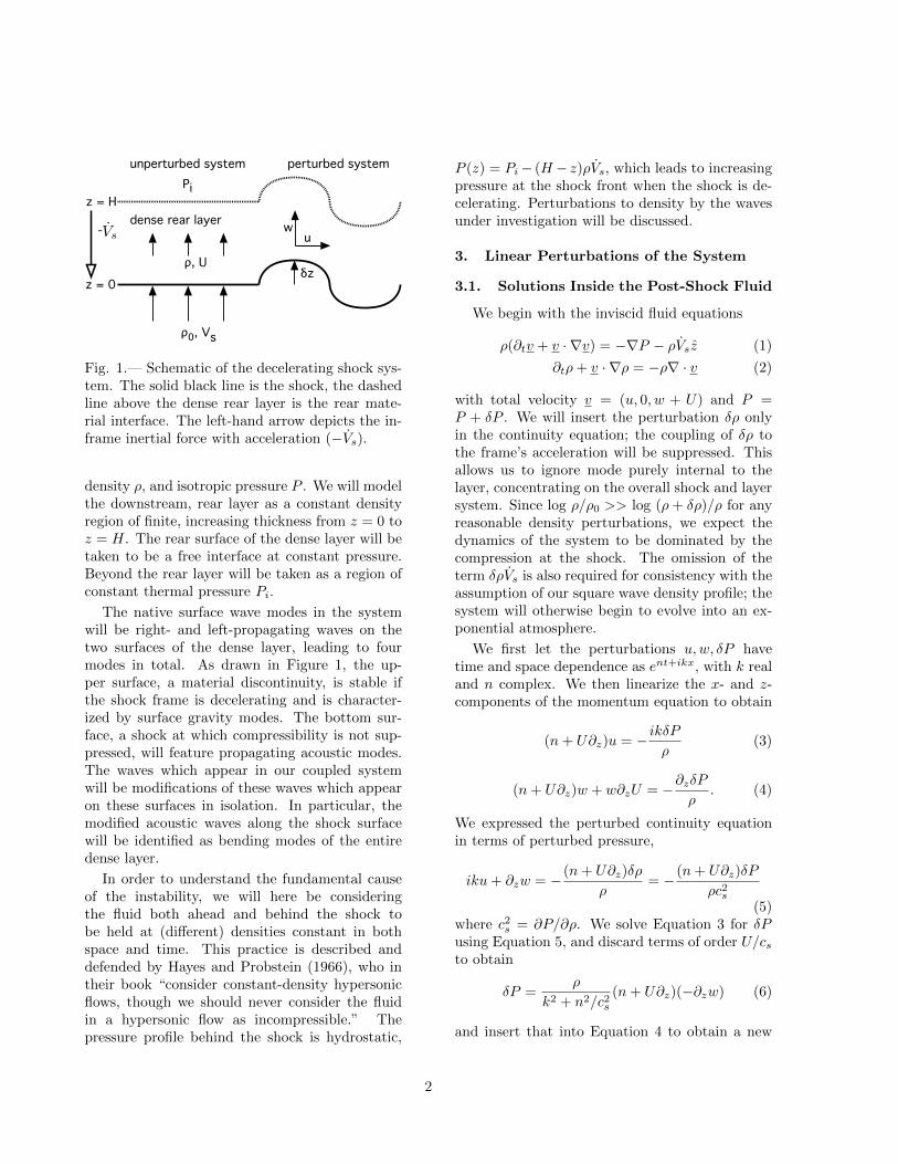
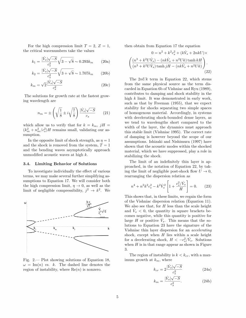
For strong shocks, T ∼ (γ + 3)/(γ + 1), in whichany effects of strong radiation are included in γas an effective polytropic index describing the to-tal density increase at the shock (Liang and Keilty2000). Z is typically close to 1. Solutions of Equa-tion 18, shown in Figure 2, yield instability fork in the range k1 < k < k2, centered around awavenumber of maximum instability km, where

k1 =|Vs|√−S

c2s

√2T − Z − 2

√T 2 − TZ (19a)

k2 =|Vs|√−S

c2s

√2T − Z + 2

√T 2 − TZ (19b)

km =|Vs|√−S

c2s

√T (19c)

We find that k1 and k2 are real for S < 0, requir-ing Vs < 0 and H < c2s/|Vs|, conditions defining adecelerating shock and a layer width shorter thana scale height.

4

For the high compression limit T = 2, Z = 1,the critical wavenumbers take the values

k1 =|Vs|√−S

c2s

√3−√

8 ∼ 0.293km (20a)

k2 =|Vs|√−S

c2s

√3 +√

8 ∼ 1.707km (20b)

km =√

2|Vs|√−S

c2s(20c)

The solutions for growth rate at the fastest grow-ing wavelength are

nm = ±

(√1

8± i√

7

8

)|Vs|√−S

cs(21)

which allow us to verify that for k = km, jH =(k2m + n2

m/c2s)H remains small, validating our as-

sumption.

In the opposite limit of shock strength, as η = 1and the shock is removed from the system, T = 1and the bending waves asymptotically approachunmodified acoustic waves at high k.

3.4. Limiting Behavior of Solutions

To investigate individually the effect of variousterms, we may make several further simplifying as-sumptions to Equation 17. We will consider boththe high compression limit, η → 0, as well as thelimit of negligible compressibility, j2 → k2. We

Vs cs

.k cs

√-S

√T

k

ω

k2k1 km

Fig. 2.— Plot showing solutions of Equation 18,ω = Im(n) vs. k. The dashed line denotes theregion of instability, where Re(n) is nonzero.

then obtain from Equation 17 the equation

0 = n2 + k2c2s + (kVs + 2nkU)×((n3 + k2UVs)− (nkVs + n2Uk) tanh kH

(n3 + k2UVs) tanh jH − (nkVs + n2Uk)

).

(22)

The 2nUk term in Equation 22, which stemsfrom the same physical source as the term dis-carded in Equation 6b of Vishniac and Ryu (1989),contributes to damping and shock stability in thehigh k limit. It was demonstrated in early work,such as that by Freeman (1955), that we expectstability for shocks separating two simple spacesof homogenous material. Accordingly, in systemswith decelerating shock-bounded dense layers, aswe tend to wavelengths short compared to thewidth of the layer, the dynamics must approachthis stable limit (Vishniac 1995). The correct rateof damping is however beyond the scope of ourassumptions. Ishizaki and Nishimura (1997) haveshown that the acoustic modes within the shockedmaterial, which we have suppressed, play a role instabilizing the shock.

The limit of an indefinitely thin layer is ap-proached, in the notation of Equation 22, by tak-ing the limit of negligible post-shock flow U → 0,rearranging the dispersion relation as

n4 + n2k2c2s − k2V 2s

[1 +

c2s/VsH

]= 0. (23)

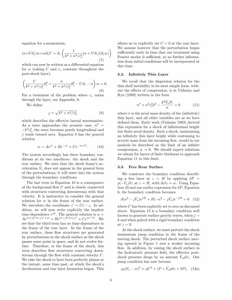
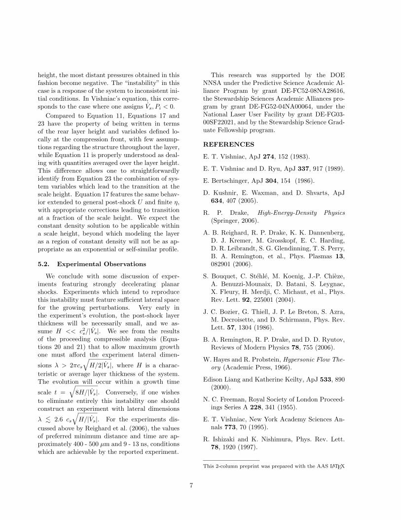
This shows that, in these limits, we regain the formof the Vishniac dispersion relation (Equation 11).We also see that, for H less than the scale heightand Vs < 0, the quantity in square brackets be-comes negative, while this quantity is positive forlarge H or positive Vs. This means that the so-lutions to Equation 23 have the signature of theVishniac thin layer dispersion for an acceleratingshock, except when H lies within a scale heightfor a decelerating shock, H < −c2s/Vs. Solutionswhen H is in that range appear as shown in Figure3.

The region of instability is k < kcr, with a max-imum growth at km, where

kcr = 2|Vs|√−S

c2s(24a)

km =|Vs|√−S

c2s. (24b)

5

Compared with Equations 20 and Figure 2, wesee that the principal result of removing the ef-fects of compressibility is to eliminate the regionof stability near k = 0. We also see that the bend-ing modes now travel asymptotically for high kwith the full speed of sound, where previously theymoved at c2s/

√T .

We note that for H << c2s/|Vs|, the rightmostterm in Equation 23 becomes very large. As Hbecomes very close to zero, one perhaps expectsthis term to level off at the value in Equation 11;we will explore this limit below.

4. Post-Shock Flow Patterns

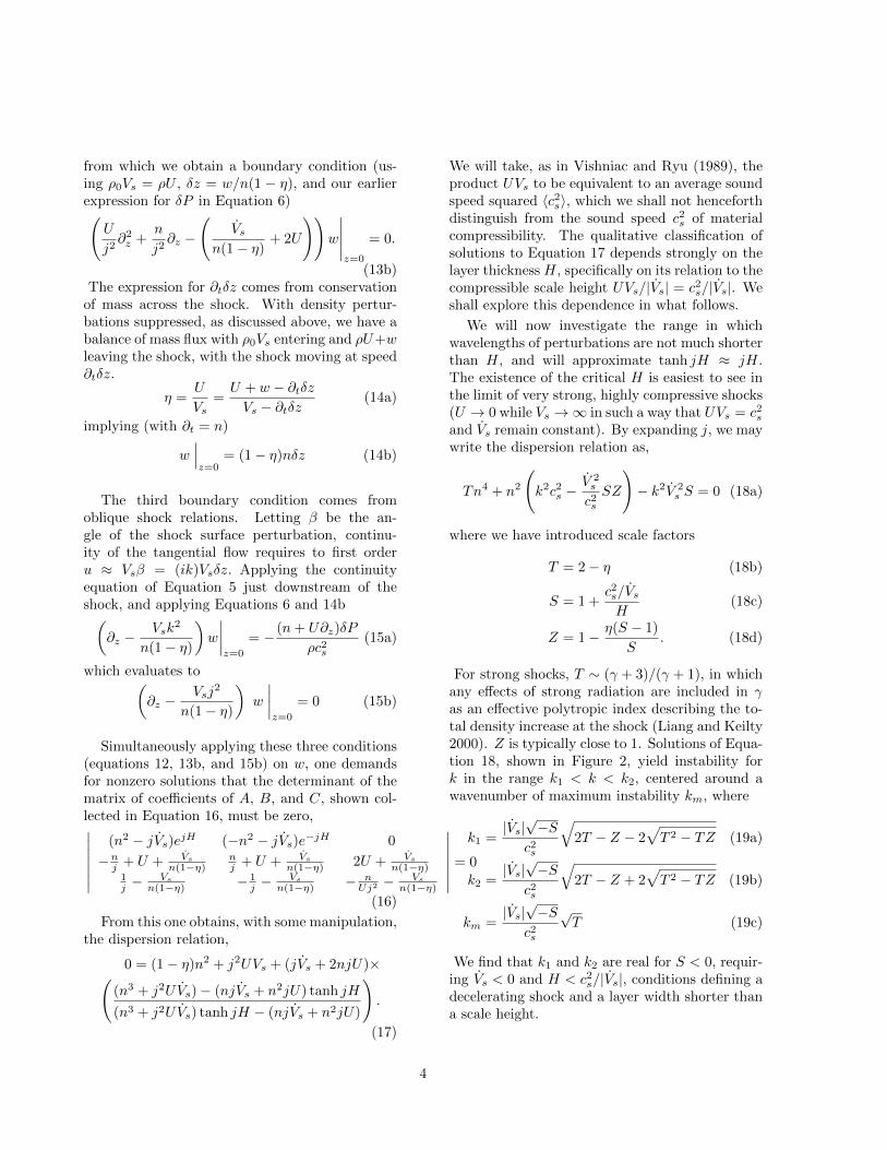
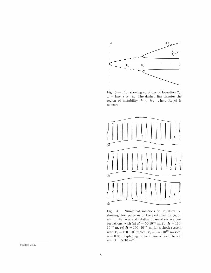
Figure 4 shows a numerical solution of Equation22 for a shock system with three different thick-nesses. The shock system has a scale height c2s/|Vs|of 144 · 10−6 m. One can see that for the very thinlayer in Fig 4(a), the flow pattern is most similarto that of a surface wave. As the post-shock layerincreases in thickness through Figs 4(b) and (c),the flow pattern evolves to contain vorticity fea-tures. We speculate that the transition at the scaleheight corresponds to a layer thickness in which acomplete cell is localized.

We remark that in the numerical solution ofEquation 22 we find that the shock and rear sur-faces’ perturbations achieve different phase. Sincethe fluid inside the layer is constant in density, thiswill lead to a corresponding perturbation of arealdensity of the layer that might be observed. Thephysical connection is therefore maintained withthe theory described by Vishniac (1983), in whichdynamics causing variation in areal density of thepost-shock layer leads to overstability in the shock.These plots may be compared with Figures 7-10 ofBertschinger (1986), which show similar vorticalstructure, though without boundary phase shift-ing.

5. Further Considerations and Conclu-sions

5.1. Connections to the Infinitely ThinSystem

We have seen that the characteristic fourth-order nature of the Vishniac instability, as de-rived in Equation 17, follows from allowing pertur-bations on both surfaces of the post-shock layer.

We note that while the Vishniac derivations con-tain an instability source in the product VsPi/σ,our dispersion relation in Equation 17 contains asource term V 2

s . This difference follows from Vish-niac’s assumption that the post-shock layer is thinand that the difference between thermal backingpressure and ram pressure together with geometricfactors (such as spherical divergence of the shock)are the fundamental sources of the deceleration.We have instead worked with planar shocks andassumed deceleration to stem primarily from massaccumulation and energy loss from the system, forexample by strong radiative cooling, and a hydro-static distribution within the layer to be the dom-inant contributor to pressure variation.

Despite these differences in approach, we can infact derive Equation 11 from Equation 23 imme-diately. We identify the sound speed at the shocksurface with local post-shock fluid variables

c2s =P (0)

ρ=Pi − ρVsH

ρ. (25)

We have implicity set the polytropic index γ = 1,which is consistent with our assumption in Equa-tion 23 that we are in the infinitely compressivelimit η = 0. However, we do not expect Equation25 to be in general consistent with our other defini-tions of c2s, except in the limit of an infinitely thinshell, H → 0. Keeping this in mind, we see thatinserting Equation 25 and σ = ρH into the term insquare brackets in Equation 23, one obtains Equa-tion 11. Our derivation therefore is found to agreewith the earlier results of Vishniac in the appro-priate limits.

We comment on the different solutions to Equa-tions 11, 18, and 23. The oscillating instabilitywhich exists when Vs < 0 is the case of interestin which collective modulation of the boundarylayers results in the growth of structure. The non-oscillating instability which appears when Vs > 0is recognized as the Rayleigh-Taylor instability ofthe rear layer under acceleration.

The non-oscillating solutions of Equations 18and 23 when Vs < 0 but H > c2s/|Vs| are of a dif-ferent nature than the other cases. The system un-der perturbation was constructed by equating thepressure P immediately behind the shock with theram pressure of the incoming material. The pres-sure profile then decreased hydrostatically withdistance from the shock. When H exceeds a scale

6

height, the most distant pressures obtained in thisfashion become negative. The “instability” in thiscase is a response of the system to inconsistent ini-tial conditions. In Vishniac’s equation, this corre-sponds to the case where one assigns Vs, Pi < 0.

Compared to Equation 11, Equations 17 and23 have the property of being written in termsof the rear layer height and variables defined lo-cally at the compression front, with few assump-tions regarding the structure throughout the layer,while Equation 11 is properly understood as deal-ing with quantities averaged over the layer height.This difference allows one to straightforwardlyidentify from Equation 23 the combination of sys-tem variables which lead to the transition at thescale height. Equation 17 features the same behav-ior extended to general post-shock U and finite η,with appropriate corrections leading to transitionat a fraction of the scale height. We expect theconstant density solution to be applicable withina scale height, beyond which modeling the layeras a region of constant density will not be as ap-propriate as an exponential or self-similar profile.

5.2. Experimental Observations

We conclude with some discussion of exper-iments featuring strongly decelerating planarshocks. Experiments which intend to reproducethis instability must feature sufficient lateral spacefor the growing perturbations. Very early inthe experiment’s evolution, the post-shock layerthickness will be necessarily small, and we as-sume H << c2s/|Vs|. We see from the resultsof the proceeding compressible analysis (Equa-tions 20 and 21) that to allow maximum growthone must afford the experiment lateral dimen-

sions λ > 2πcs

√H/2|Vs|, where H is a charac-

teristic or average layer thickness of the system.The evolution will occur within a growth time

scale t =√

8H/|Vs|. Conversely, if one wishes

to eliminate entirely this instability one shouldconstruct an experiment with lateral dimensions

λ . 2.6 cs

√H/|Vs|. For the experiments dis-

cussed above by Reighard et al. (2006), the valuesof preferred minimum distance and time are ap-proximately 400 - 500 µm and 9 - 13 ns, conditionswhich are achievable by the reported experiment.

This research was supported by the DOENNSA under the Predictive Science Academic Al-liance Program by grant DE-FC52-08NA28616,the Stewardship Sciences Academic Alliances pro-gram by grant DE-FG52-04NA00064, under theNational Laser User Facility by grant DE-FG03-00SF22021, and by the Stewardship Science Grad-uate Fellowship program.

REFERENCES

E. T. Vishniac, ApJ 274, 152 (1983).

E. T. Vishniac and D. Ryu, ApJ 337, 917 (1989).

E. Bertschinger, ApJ 304, 154 (1986).

D. Kushnir, E. Waxman, and D. Shvarts, ApJ634, 407 (2005).

R. P. Drake, High-Energy-Density Physics(Springer, 2006).

A. B. Reighard, R. P. Drake, K. K. Dannenberg,D. J. Kremer, M. Grosskopf, E. C. Harding,D. R. Leibrandt, S. G. Glendinning, T. S. Perry,B. A. Remington, et al., Phys. Plasmas 13,082901 (2006).

S. Bouquet, C. Stehle, M. Koenig, J.-P. Chieze,A. Benuzzi-Mounaix, D. Batani, S. Leygnac,X. Fleury, H. Merdji, C. Michaut, et al., Phys.Rev. Lett. 92, 225001 (2004).

J. C. Bozier, G. Thiell, J. P. Le Breton, S. Azra,M. Decroisette, and D. Schirmann, Phys. Rev.Lett. 57, 1304 (1986).

B. A. Remington, R. P. Drake, and D. D. Ryutov,Reviews of Modern Physics 78, 755 (2006).

W. Hayes and R. Probstein, Hypersonic Flow The-ory (Academic Press, 1966).

Edison Liang and Katherine Keilty, ApJ 533, 890(2000).

N. C. Freeman, Royal Society of London Proceed-ings Series A 228, 341 (1955).

E. T. Vishniac, New York Academy Sciences An-nals 773, 70 (1995).

R. Ishizaki and K. Nishimura, Phys. Rev. Lett.78, 1920 (1997).

This 2-column preprint was prepared with the AAS LATEX

7

macros v5.2.

Vs cs

.

k cs

√-S

k

ω

kcrkm

Fig. 3.— Plot showing solutions of Equation 23,ω = Im(n) vs. k. The dashed line denotes theregion of instability, k < kcr, where Re(n) isnonzero.

(a)

(b)

(c)

Fig. 4.— Numerical solutions of Equation 17,showing flow patterns of the perturbation (u,w)within the layer and relative phase of surface per-turbations, with (a) H = 50·10−6 m, (b) H = 110·10−6 m, (c) H = 190 · 10−6 m, for a shock system

with Vs = 120 · 103 m/sec, Vs = −5 · 1012 m/sec2,

η = 0.05, displaying in each case a perturbationwith k = 5210 m−1.

8

A. Compressible Rear Layer

We wish to extend the results of Section 3.1 to the investigate the case where the speed of sound variesthrough the dense layer. Previously, we assumed a hydrostatic pressure profile on an isothermal layer, whichimplies the speed of sound varies as

c2s = c2s(z) = cs20 + γVsz (A1)

where γ is the polytropic index of the layer, and cs20 is the speed of sound immediately behind the shock

wave. We revisit the differential equation from 7,

(n+ U∂z)w = ∂z

(1

k2 + n2/c2s(z)(n+ U∂z)(∂zw)

)(A2)

where we are now treating c2s as a function of z.

In order to investigate solutions to A2, we must first realize that our perturbation ansatz ent+ikx is nolonger valid; either n or k must also vary as a function of z. Since n is our variable of interest, we select k tobecome k(z). We assume that relation between k and n will be linear in cs. We model the effect by defining

Γ2 = k2(z)cs(z)2 + n2 (A3)

where Γ is assumed constant. We can then rewrite Equation A2 as(Γ2 − γVs∂z −

(cs

20 + γVsz

)∂2z

)(n+ U∂z)w = 0. (A4)

We identify the two differential operators

DB =(

Γ2 − γVs∂z −(cs

20 + γVsz

)∂2z

)(A5)

Dt = (n+ U∂z) (A6)

and rewrite Equation A4 asDBDtw = 0. (A7)

It is known from the theory of differential equations that a differential equation in the form above has asits general solution the sum of general solutions of its component operators if they are permutable. Thecommutator of our operators is nonvanishing, but

[DB , Dt] = γVsU∂2z (A8)

will be neglected, anticipating that we will eventually take the limit of U going to zero.1

Having eliminated the commutator, one may then consider the sum of general solutions of each indepen-dent operator as the complete general solution to the combined equation. The general solution for Dt isCe−nz/U . The general solution of DB can be found by a change of variables to

ζ = 2

√Γ2cs2(z)

γ2V 2s

to cast DB as

DB = −Γ2

(∂2ζ +

1

ζ∂ζ − 1

)(A9)

1 If we do not accept the approximate permutability of DB and Dt, our general solution is found, by use of integrating factors,to be

w = e−nz/U ·1

U

(∫enz/UA′ I0

(2

√Γ2c2s(z)

γ2V 2s

)+B′ K0

(2

√Γ2c2s(z)

γ2V 2s

)dz

)+ C′e−nz/U .

The arbitrary constants are written with primes to distinguish them from the approximate case.

9

which is the operator corresponding to the modified Bessel equation. Solutions to DB are of the form

A I0

(2√

Γ2c2s(z)

γ2V 2s

)+B K0

(2√

Γ2c2s(z)

γ2V 2s

), where I0 and K0 are the modified Bessel functions.

We take as our approximate general solution

w = A I0

(2

√Γ2c2s(z)

γ2V 2s

)+B K0

(2

√Γ2c2s(z)

γ2V 2s

)+ Ce−nz/U . (A10)

The new basis for w written with modified Bessel’s functions is less dissimilar to the previous basis, Equation10, than it appears at first glance. To first order in δs and zeroth order in U/cs, the differential forms of theboundary conditions are changed only cosmetically.

0 =(n2c2s(z)∂z − Γ2Vs

)w∣∣∣z=H

(A11a)

0 =

(Uc2s(z)

Γ2∂2z +

nc2s(z)

Γ2∂z −

(Vs

n(1− η)+ 2U

))w

∣∣∣∣∣z=0

(A11b)

0 =

(c2s(z)

Γ2∂z −

Vsn(1− η)

)w

∣∣∣∣z=0

(A11c)

To obtain the dispersion relation from the boundary conditions, we note that

j(H) = j(0)cs0cs(H)

= j(0)

√1− γVsH

c2s(H).

and evaluate w to obtain∣∣∣∣∣∣∣∣∣∣∣∣

n2K1(ζH)− jVsK0(ζH) cs0

cs(H) −n2I1(ζH)− jVsI0(ζH) cs0

cs(H) 0

−nj(

1− γ UVs

nc2s0

)K1(ζ0)

+(U + Vs

n(1−η)

)K0(ζ0)

nj

(1− γ UVs

nc2s0

)I1(ζ0)

+(U + Vs

n(1−η)

)I0(ζ0)

2U + Vs

n(1−η)

1jK1(ζ0)− Vs

n(1−η)K0(ζ0) − 1j I1(ζ0)− Vs

n(1−η)I0(ζ0) − nUj2 −

Vs

n(1−η)

∣∣∣∣∣∣∣∣∣∣∣∣= 0. (A12)

In Equation A12, j = j(0), ζH = 2√

Γ2c2s(H)

γ2V 2s

, and ζ0 = 2

√Γ2cs2

0

γ2V 2s

.

Equation A12 reduces to the dispersion relation with constant speed of sound in the limit of γ → 0. Wesee that the only substantial changes are in the terms incorporating the effect of layer height H and the

appearance of two terms of γ UVs

nc2s. The latter of these is the same term which was neglected previously in

writing Equation A8, and will be neglected here for consistency.

In analogy to Section 3.3, we take the limit of U → 0, Vs → ∞, UVs → c2s0, and write the dispersionrelation as

0 = (1− η)n2 + j2c2s0 + jVs

(n2 − jVsF1

n2F2 − jVsF3

)(A13a)

where

F1 =I0(ζ0)K0(ζH)−K0(ζ0)I0(ζH)

I0(ζ0)K1(ζH) +K0(ζ0)I1(ζH)

cs0

cs(H)(A13b)

F2 =I1(ζ0)K1(ζH)−K1(ζ0)I1(ζH)

I0(ζ0)K1(ζH) +K0(ζ0)I1(ζH)(A13c)

F3 =I1(ζ0)K0(ζH) +K1(ζ0)I0(ζH)

I0(ζ0)K1(ζH) +K0(ζ0)I1(ζH)

cs0

cs(H)(A13d)

10

Compared to the previous dispersion relation in Equation 17, F1 and F2 are analogous to tanh(jH) andF3 was previously equal to one. These identities are preserved if we assign the cylinder functions I0,1(ζ0) =1, I0,1(ζH) = e−jH , K0,1(ζ0) = 1,K0,1(ζH) = ejH , and γ = 0 (and therefore cs(H) = cs0).

The effects of the changing speed of sound can be approximately included in, for example, Equation 23,by writing

n4 + n2k2cs20 −

cs0

cs(H)k2V 2

s

[1 +

c2s/VsH

]= 0 (A14)

where k = k|z=0. The diminishing speed of sound with rising layer height evidently amplifies the instability.Physically, this comes from the fact that for a given n, the wavelength of sound waves will be shorter inthe region of lower sound speed. This leads to an increased k on the rear, instability-forming boundarycondition.

11