ebpa: an efficient data structure for frequent closed itemset mining

Applied Mathematical Sciences, Vol. 7, 2013, no. 30, 1483 - 1506 HIKARI Ltd, www.m-hikari.com

EBPA: An Efficient Data Structure

for Frequent Closed Itemset Mining

Chakarin Vajiramedhin

Department of Computer Science, Faculty of Science

King Mongkut’s Institute of Technology

Ladkrabang, Bangkok, 10520, Thailand

[email protected]

Jeeraporn Werapun

Department of Computer Science, Faculty of Science

King Mongkut’s Institute of Technology

Ladkrabang, Bangkok, 10520, Thailand

[email protected]

Copyright © 2013 Chakarin Vajiramedhin and Jeeraporn Werapun. This is an open access

article distributed under the Creative Commons Attribution License, which permits unrestricted

use, distribution, and reproduction in any medium, provided the original work is properly cited.

Abstract

In closed itemset mining, the process of mining from a large transaction database

directly often leads to inefficient space and time. Practically, many data structures

were proposed to maintain valuable data for frequent closed itemset mining

(FCIM), while each data structure has its own advantages and disadvantages. In

recent study, a collaboration of array, bitmap, and prefix tree was proposed to gain

advantages of those basic data structures by reducing the computing time of the

FCIM. That collaboration can save space over that of the original prefix tree,

which requires extra space for (m-1) parent-child pointers and its corresponding

hashing table (in each tree-node). However, the extra sorting all transactions and

merging repeated transactions are required before constructing the prefix tree.

Therefore, this paper presents the improved collaboration data structure, called the

EBPA (Efficient Bitmap-Prefix-tree Array), with the efficient (parent-child)

access in O(1) by using a (temporary) pointer array (without space for hashing)

and not require the extra sorting transactions. In system performance evaluation,

experimental results showed that the response time of our EBPA-based FCIM

mining outperforms over that of the existing collaboration-based FCIM approach.

1484 C. Vajiramedhin and J. Werapun

Keywords: data mining, closed itemset mining, bitmap-prefix-tree array data

structure

1 Introduction

Frequent Closed Itemset Mining (FCIM) is the main important technique in

several data mining applications (e.g., classifiers, association rules, etc.), for

representing useful extracting patterns (or itemsets) from all of very large

candidate patterns within a transaction database for solving the problem of a

frequent itemset mining (FIM). The FIM approaches are possible to create an

exponential number of output patterns, especially in case of the minimum support

threshold is set to low value, while the transaction database is very large. Later

research focuses on the complete closed itemsets, which can reduce a number of

itemsets without information loss and can represent covering all results of the

original FIM with saving memory space and time. Therefore, many FCIM

approaches have been proposed [1] - [14].

Besides the best solution, an appropriate data structure and corresponding

frequency computation functions are a key to improve the performance of each

method. Recently, many data structures for computing the FCIM have been

proposed ([4], [7], [10], [12], [14]).

In 2002, CHARM algorithm and IT-TREE data structure [4] were proposed

for finding frequent closed itemsets. That approach is efficient in frequency

counting over FCIM with using inverted lists data structure. However, it requires

large memory space for storing node information ((m-1) pointers and its hashing).

The frequency computation and the closure process of that prefix tree approach

are still the heaviest task of the FCIM, especially the process of the longest path of

the prefix tree (≤ m items).

In 2003, the array list data structure was introduced to support LCM approach

[7], by storing each transaction of the database in the array lists. That array

list-based method is efficient in computation for a sparse transaction database, but

it is still weak in a dense transaction database [10].

In 2006, the vertical bitmap data structure was improved over the original

bitmap to support DCI-CLOSED approach [12]. That data structure is efficient in

memory space for the dense transaction database, especially to save memory in

storing data by using only one bit (0 or 1) for each item, represented in all

itemsets. However, that method may not be efficient in time (O(mT2)) in the

sparse transaction database since its corresponding bitmap matrix containing

many 0s but the process is equal to mT2 fixed steps, where m is a number of

frequent 1-itemset and T is a number of transactions in the database.

The collaboration of array lists, vertical bitmap, and prefix-tree data structure

[10] was proposed in 2005 to utilize the advantages of those basic data structures

for making more efficient in computation time and saving more memory space.

In particular, the (compact) prefix tree and (bucket) array lists are combined to

EBPA: an efficient data structure for frequent closed itemset mining 1485

reduce the FCIM computing time over that of the (original) prefix tree in

CHARM [4] and the array list in LCM [7]. In addition, using the bitmap

(transaction) node and no extra space for (m-1) parent-child pointers and hashing

(in each node). So far, the collaboration method is efficient but it requires time

to sort all transactions and combine the repeated transactions before constructing

the prefix tree (from the leaf nodes to the root), corresponding to the specific

transaction order.

In this paper, we propose the improved collaboration data structure, called the

EBPA (Efficient Bitmap-Prefix-tree Array) and the EBPA-CLOSED algorithm

for frequent closed itemset mining. The EBPA data structure, the (top down)

prefix-tree construction, is an improved version of our previous work, the (bottom

up) prefix-tree BPA [14]. In order to gain the advantage of the collaboration

approach, our EBPA maintains all features and results of the existing

collaboration data structure [10] without extra sorting and merging transactions.

In our EBPA data structure, the efficient (parent-child) access is introduced in O(1)

time by using a temporary pointer array (in each node) but no hashing space and

(a) (b) (c)

(d) (e)

Fig. 1 a) an original transaction dataset, containing four 1-itemsets (a, b, c and d) and existing data structures represent nine transactions, b) Vertical Bitmap Matrix, c) Array List, d) Prefix tree, and e) Collaboration (Array, Bitmap, Prefix tree).


no extra sorting all transactions. Our method provides not only saving space but

also saving time that is faster and easier to access each (parent-child) node of the

prefix-tree array for filling and counting the frequency. Finally, like the existing

collaboration, the result of our EBPA provides the faster computing in item-based

buckets (arrays) for the closure process of the FCIM mining. In addition to

saving space, we design the EBPA that creates the compact prefix tree, containing

only occurrence nodes from the transaction database (with storing 2 integers (tid

and w) in each node) and uses the shared (bitmap) itemsets among corresponding

nodes along the same path (of the prefix tree) for saving more space.

The remainder of this paper is organized as follows: Section 2 provides a

concise survey of related work. Section 3 presents our efficient EBPA data

structure and the EBPA-CLOSED algorithm for the FCIM mining. Section 4

displays the performance evaluation and experimental results. Finally, conclusion

and future study are discussed in Section 5.

2 Related Work

The FCIM, first proposed by Pasquier et al.[1] in 1999, is an interesting

alternative solution for representing useful extracting patterns from very large

candidate patterns within transaction database. The FCIM is known as an

efficient mining technique because of interesting only the frequent closed itemsets

instead of mining the complete set of frequent itemsets. The complete itemsets

derived from this method can reduce a number of itemsets without information

loss, where as it can represent or cover all results of the original FIM. Therefore,

the FCIM approach saves more time to search only the frequent closed itemsets

without using a huge space for keeping all result patterns.

Let D = {t1, t2, t3, …, tT} be a transaction database. Each ti is a transaction (i =

1, 2, 3, …, T) in the database consisting of a transaction identifier (tid) and items

ordered from 1 to k items (i1, i2, i3, …, ik).

Definition 1: Let I = (i1, i2, i3, …, ik) be a set of items in transaction database that

every subset P of I is called an itemset. The itemset P with k items is called a

k-itemset. The number of transaction in D matching the itemset P is called the

support of P, denoted as supp(P). Given a minimum support threshold min_supp,

the itemset P is called a frequent itemset if and only if supp(P) ≥ min_supp.

Example 1: Form input transaction database in Fig.1a, there are four 1-itemsets (a,

b, c, and d)) and suppose minimum support threshold is 5. The frequent 1-itemsets

are (a:9), (b:6), (c:6) and (d:5). Therefore a set of frequent itemsets is {(a:9), (b:6),

(c:6), (d:5), (ab:6), (ac:6), (ad:5), (abc:5)}, because their occurrences (or support)

are equal to or more than 5 (support ≥ 5) that pass the minimum support threshold.

Definition 2: The itemset P is a closed itemset if there is no superset and can

represent all itemsets that belong to the same equivalence class with the same


support. A closed itemset P is frequent if its support passes the given support

threshold (supp(P) ≥ min_supp).

Example 2: From input transaction database in Fig.1a, suppose minimum support

threshold is 5. The itemsets a:9, ab:6, ac:6, ad:5, and abc:5 are called the closed

frequent itemsets (see Fig.2), because their occurrences are equal to or more than

5, passing the given support threshold, and can represent the belonging itemsets in

the same equivalence class with the same support.

Fig.2 shows the lattice of frequent itemsets and closed frequent itemset

derived from the input transaction database from Fig.1a. For example, the itemset

cab:5 is a closed frequent itemset, because it can represent itemsets c:5, ca:5, cb:5,

and cab:5, etc. That approach collects five itemsets only, instead of storing all

itemsets, and hence can save more space. The closed itemsets are the results of the

frequent closed itemsets mining (FCIM) representation of all frequent itemsets in

the same support of equivalence class extracted from the transaction database. In

the past ten years, many FCIM techniques [4], [7], [10], [12] were proposed to

solve the data storage problem with compacted data by storing a set of

representative itemsets that can cover all other itemsets. Each technique has its

specific function and data structure that have some advantages and disadvantages

to tradeoff. The performance keys of each technique are the efficient data

structure construction, including the fast frequency computation function.

The vertical bitmap data structure was developed to support DCI-CLOSED

approach [12] (Fig.1b) and its efficacious FCIM traversed the search space in a

depth-first manner. This data structure is a memory space efficient structure for

the dense transaction database, especially in saving memory to store data in main

memory that represents all itemsets in the input transaction database by using only

one bit (0 or 1) for each item (or mT bits for all transactions (T)), where m

represents a number of frequent 1-itemsets. However, this method may not be

efficient in time (O(mT2)) for the sparse transaction database since its

corresponding bitmap matrix containing many 0s but the process is always equal

to mT2 iterations. Therefore, that data structure will take long time to compute the

frequency of itemsets in case of there are a lot of transactions (T) in the database

where as there are a few number of items in each transaction.


The array list data structure was used to support the original LCM [7]. In this

(inverted) list-based approach (Fig.1c), each of T transactions in the database is

scanned and stored in frequent 1-itemset buckets in O(mT) (see Fig.1c). A number

of array lists are equal to the number of the frequent 1-itemset (m) and the length

of each array is equal to the frequency of each 1-itemset. The array list data

structure computes the frequencies of itemsets by scanning from the lists of the

1-itemset in m buckets. Thus, the array list-based method yields an efficient

computation for a sparse transaction database, but it is still weak in any dense

transaction database.

The IT-TREE data structure (see Fig.1d) and CHARM algorithm [4] were

proposed for finding frequent closed itemsets. The process of that approach is

based on the prefix tree and (parent-child) hashing for support both dense and

sparse transaction databases that store an itemset (≤ m bytes) in each node of the

prefix tree, where m is a number of frequent 1-itemsets. Each node of the tree

contains an item identifier (≤ m bytes), a support (or frequency), a parent-node

pointer, child node indices (≤ m), and a hashing table. The prefix tree is

constructed from the root and the first level contains 1-itemsets only and their

(inversed-list) frequency counting for T transactions in O(mT), where m is a

number of levels (for m 1-itemsets). More time are required for adding all

corresponding nodes (in other levels) of the prefix tree. The main advantage of

using IT-TREE in CHARM is that frequent searching with the hashing

(parent-to-child nodes) is efficient. However, that approach may require large

memory space for storing node information (in bytes) in all nodes (n ≤ N = 20 + 2

1

+…+ 2m-1

= 2m - 1). The frequency computation and the closure process of that

prefix tree are still the heaviest task of the FCIM mining, especially the process of

the longest path of the prefix tree (≤ m items).

Lately, the collaboration data structure [10] was introduced (see Fig.1e) to

combine three basic data structures (array lists, vertical bitmap, and prefix tree) to

utilize advantages of each data structure for making more efficient in computation

time and saving more memory space. Such a collaboration data structure was

developed to support the efficient LCM (version 3) for mining large transaction

Fig.2 A lattice of the frequent closed itemset (min_supp=1) mine the input data

from Fig.1a.


database, including dense and spare databases. In that collaboration, the (compact)

prefix tree and (bucket) arrays are combined to save time of frequency computing

and closed processing over that of the (original) prefix tree in CHARM [4] and the

array list in original LCM [7]. In addition, the (bitmap) transaction in each

tree-node is used to save space over the construction of the prefix tree in CHARM

(since there is no extra space required for (m-1) parent-child pointers and hashing

(in each node)). However, that collaboration approach requires the extra sorting

of all T transactions (m elements per transaction), according to decreasing order of

levels and prefix items in O(mT), to merge the repeated transactions before

constructing the (bottom up) prefix tree, corresponding to that transaction order.

After merging the repeated transactions, the collaboration data structure is created,

as follows: Each of T′ (≤ T) unique transactions is scanned to fill its initial

frequency into the corresponding node (of the prefix tree), containing an m-bitmap

array and a weight) from leaf nodes to the root) in O(T′). During move to fill

frequency of nodes in the next (lower) level (of m levels), the frequency of each

child node is shared to corresponding parent nodes (for m levels (ni nodes in each

level i)). Therefore, time complexity of the collaboration to construct the

(compact) prefix tree is O(mT) + O(mniT’), where n = max(ni), ni ≤ 2i and i = 0, 1,

2, … , m-1. In addition, to save space, that data structure stores bitmap-itemsets

in binary (0/1) format, like the vertical bitmap, in each node of the prefix tree.

Next process is performed in separate array buckets, which store only occurrence

(transaction) nodes and process the frequency counting of the remaining itemsets

in the buckets for efficient FCIM mining. Finally, the efficient FCIM processing

in LCM3 is computed by applying the ppc-extension (prefix preserving closure

process) algorithm [11] and the collaboration data structure [10]. Practically, the

collaboration approach is efficient for the FCIM mining since using bitmap-node

(without (m-1)-pointers) to save memory space and using prefix-tree plus bucket

arrays to save processing time of the FCIM mining. However, the response time

of that collaboration in LCM3 can be improved if its process does not require

extra sorting to order all T transactions before constructing the prefix tree.

3 The improved Collaboration (EBPA) Data Structure for FCIM

Mining

In this section, we present the improved collaboration data structure, called “the

EBPA (Efficient Bitmap Prefix-tree Array) data structure” based on the efficient

(parent-child) access of the prefix-tree array in O(1) and the EBPA-CLOSED

algorithm to improve both time and space for the FCIM mining. The contribution

of our FCIM mining includes the following functions:

1. Propose the (parent-child) access (O(1)) for the (compact) prefix tree (in

Section 3.1).


2. Design the efficient EBPA data structure that utilizes the (compact) prefix tree

and (bucket) arrays with no extra sorting before constructing the prefix tree (in

Section 3.2).

3. Improve the ppc extension [11] for the FCIM mining with the pre-test

technique to look over unnecessary closure sets and post sets and save the

response time of the FCIM computing (in Section 3.3).

3.1 The (Temporary) Pointer Array for Efficient Parent-Child Access: O(1)

Fig.3a illustrates an example of the (compact) prefix tree (of four items (a, b, c,

d)) that node indexing (in each level) are assigned corresponding to order of

incoming transactions. Fig.3b depicts the (complete) prefix tree, where node

indexing (in each level i) are assigned with prefix ordering (0, 1, 2, …, ni-1, where

ni = a number of nodes in level i (= 2i) and i = 0, 1, 2, … , m-1. Practically, the

(compact) prefix tree requires a counter (ci) in each level i to set index (for each

bucket array without any fragment) and hence the number of occurrence nodes (ni

≤ 2i) in each level i can be linear up to exponential nodes.

Let b0b1b2 … bm-2bm-1) represent the (bitmap) transaction or itemsets.

ptr represent a (temporary) pointer array with O(1) access (equation (1)).

lp represent the level of the parent node, where lp = p and 0 ≤ p ≤ m-1.

li represent the level of the child node, where li = i ( > p) and 0 < i ≤ m-1.

ci represent the counter for setting (compact) node-index in each level i.

(a) (b)

Fig.3 The prefix-tree array of four items (a, b, c, d): a) the (compact) prefix tree

(with non-order index), b) the (complete) prefix tree (with prefix-order index).

During construction of the (compact) prefix tree, the (temporary) pointer array

(ptr) is required for each (internal) occurrence node. A number of child nodes for

a parent are m-p-1 nodes, depending on a number of items (m) and prefix-items

upto the parent node (p). The location of that pointer array (m-p-1 elements) for

each particular parent-child can be 0, 1, 2,…, or m-p-2, as defined in equation (1).

�� 1,��#�� 1 (1)

For each (bitmap) transaction, the lptr (in equation(1)) is computed in O(1) to

point to corresponding child directly, related to levels of child (li = i) and parent

(lp = p), illustrated in Table 1 for all internal nodes of the prefix tree.


Table 1. The (temporary) pointer array for all (internal) nodes of the prefix tree.

node bitmap level p li=i location of ptr

a

1000

0

i=1

i=2

i=3

lptr =1-0-1 = 0

lptr =2-0-1 = 1

lptr =3-0-1 = 2

ab

1100

1

i=2

i=3

lptr =2-1-1 = 0

lptr =3-1-1 = 1

b

0100

1

i=2

i=3

lptr =2-1-1 = 0

lptr =3-1-1 = 1

abc

1110

2

i=3

lptr =3-2-1 = 0

ac

1010

2

i=3

lptr =3-2-1 = 0

bc

0110

2

i=3

lptr =3-2-1 = 0

c

0010

2

i=3

lptr =3-2-1 = 0

3.2 The Construction of the EBPA Structure

We design the efficient EBPA data structure as an array-based (compact) prefix

tree for saving space (in practice) that concerns only occurrence transactions and

their corresponding parent nodes, an improved version of our previous data

structure (BPA) [14] that exponentially generates full nodes (N) of the complete

prefix tree (Fig.3b), where N = 20 + 2

1 + 2

2 + … + 2

i + … + 2

m-1 = 2

m – 1 nodes.

In particular, there are two main steps in the collaboration based EBPA-FCIM

mining: 1) create the (compact) prefix tree (Fig.4b) and the (bucket) arrays (Fig.4c)

in Section 3.2 and 2) compute the closure sets and post sets of the FCIM mining

(see Section 3.3). Our focus in this section is the first part, the EBPA (Efficient

Bitmap-Prefix tree Array) data structure, which is introduced to improve space

and time of the construction of the (compact) prefix tree array (from T

transactions directly without extra sorting), while yielding similar results to the

original collaboration in LCM3 [10]. In our EBPA structure, the (temporary)

pointer array ptr (of m-p-1 elements with initially setting to -1) is introduced with

efficiently accessed in O(1) by using a specific location lptr (equation(1)) and a

counter (ci) in each level i to access parent-child nodes (< m) (without hashing).

Note that the initial counter ci is set to -1 (ci = -1) and it is incremented by one

(++ci) before adding the new node (in level i) for the corresponding transaction.

Therefore, time complexity of the frequency computing (along the same path) for

each transaction is O(m) for existing nodes and O(m2) for new nodes and for all T

transactions is O(m2n) + O(mT), where n = max(ni) and n ≤ 2

i, i = 0, 1, 2, … , m-1.


(a) (b) (c)

Fig.4 Our EBPA data structure: a) the input dataset; b) the (compact) prefix tree;

and c) the (bucket) arrays.

The compact prefix-tree array (Fig.4b) is an associative array that a number of

levels in prefix array are equal to a number of 1-itemsets (i.e., a, b, c, d). Each

node contains only a support (weight w) and a transaction id (tid) to the shared

bitmap array of the same branch of the prefix-tree array. In our approach, the

bitmap-array table (Fig.4a) contains a number of shared bitmaps (0/1) of related

transactions or nodes along the same path in the prefix tree (i.e., a shared bitmap

1111 for itemsets abcd (4 bits) upto level 3, abc (3 bits) upto level 2, ab (2 bits)

upto level 1, and a (1 bit)) in level 0. The size of the bitmap array is T×m, where T

is a number of transactions in database and m is a number of 1-itemsets that their

support values ≥ min_supp. The construction of our EBPA data structure is

illustrated in Algorithm 1, which composes of two main steps:1) the initial

process and 2) the EBPA construction.

First, step 1.1 loads the input file to initialize memory and scans all

transactions (in the database) for finding frequency of each item (fi), m 1-itemsets,

Algorithm 1: Constructing of EBPA data structure.

Step 1: Initial process [O(kT)]

1.1 scan all transactions to find some parameters: T (#transactions), k (#all itemsets), f (frequency of each item), l (level of each

transaction), and set minimum support threshold to find m (#frequent itemsets). 1.2 sort m frequent itemsets in descending order of item- frequency.

1.3 convert all T transactions in a bitmap 0/1 format (m-bit).

Step 2: EBPA construction [O(m2n) + O(mT)]

2.1 start with scanning (bitmap) transaction for finding the level (i) containing 1-bit. 2.2 check in level i of (compact) prefix array whether there exists that node or not.

if yes (i.e., identifier ≥ 0), increment frequency; otherwise (i.e., identifier =-1) create node and set node information (tid, w, m-p-1 (temporary) pointers).

2.3 set current node to be parent (level p) and scan next 1-bit (level i) and apply eq.(1) (location of ptr = i-p-1) to link to child node (level i) and

repeat step 2.2 – 2.3 until the end of transaction. 2.4 move to the next transaction and repeat step 2.1 - 2.4 until the last transaction.


a number of transactions (T). Then, step 1.2 sorts m frequent itemsets in

descending order of item-frequency. Next, step 1.3 allocates the bitmap array and

set 0 to initialized data. Then, scan all transactions by m frequency order pattern

and set 1 into bitmap array in the frequent items. For example, Fig.4a illustrates

the bitmap array, the results of step 1 ready to generate the EBPA data structure.

In step 2, the existing collaboration [10] requires extra sorting T transactions

(m-bit itemset per transaction) and their merging the same repeated transactions.

Its prefix-tree arrays are constructed (i.e., fills the frequency back) from level m-1

(leaf nodes) to level 0 (the root), according to sorted (T’) unique transactions.

Applying the compact prefix-tree array of that collaboration may confront with

many difficulties (i.e., requiring extra sorting, finding child-parent relation, etc.)

and take long time in cases of a large amount of 1-itemsets to build the prefix-tree

array. In our top-down EBPA approach (with our efficient parent-child access in

O(1)), we construct the compact prefix-tree array (without extra sorting) by

storing only occurrence transactions and their parent nodes. In our approach, fill

frequency processing time depends on a number of occurrence items (≤ m) in each

transaction. Thus, time complexity of filling frequency for each transaction is

O(m) for existing nodes or O(m2) for new nodes (with m-p-1 temporary pointers

per node) and O(m2n) + O(mT) for all T transactions and there exist n nodes in the

(compact) prefix tree. In step 2.1, we start with scanning the bitmap transaction

for finding the level containing the first 1-bit, representing the first item of that

transaction (i.e., assume level i). Next, step 2.2 checks in level i of the compact

prefix array whether the current node was created in the level i or not. If that node

does not exist, increment the counter of level i (++ci), create that node in level i

(at index = ci) and set information (i.e., a transaction id number (tid), the support

(weight=1)), and allocated the (temporary) pointer array (ptr) to link to its (m-p-1)

child nodes with initial setting to (-1). In case of that node was created already,

increment frequency (or weight) in that child node. Then, step 2.3 sets the

current node to be the next parent (in level p) and scans the same transaction to

find out the level of the next 1-bit (i.e., level i > p). From the parent node (in level

p) and the particular child (in level i), apply equation (1) to jump to that child

node directly. Then, repeat step 2.2–2.3 for the next item (or 1- bit) until the end

of transaction. Next, move to the next transaction and repeat the same process

(step 2.1–2.4) until the end of dataset (with the last transaction). Lastly, free the

(temporary) bucket array for returning the memory space.

In our EBPA data structure, the (compact) prefix tree array is constructed for

each of nine transactions (tid0 – tid8) of the input dataset (Fig.4a), as follows:

For each tid 0 – 1 (abcd: 1111), the 1st and 2

nd items are a (parent, level p=0)

and b (child, level i=1) and hence the location of ptr = i – p – 1 = 1-0-1 = 0 (that is

ptr[0] = ++c1 = 0) and then weight w of node[c1=0] in level 1 is incremented. Next

child of that itemset is c (level i=2) with parent b (level p=1) and the location of

ptr = i – p – 1 = 2-1-1 = 0 (that is ptr[0] = ++c2 = 0) and then weight w of

node[c2=0] in level 2 is increased. Finally, last child of that itemset is d (level i=3)

with parent c (level p=2) and the location of ptr = i – p – 1 = 3-2-1 = 0 (that is

ptr[0] = ++c3 = 0) and then weight w of node[c3=0] in level 3 is increased.


Next, for tid 2 (abd: 1101), the first and second items are a (parent, level

p=0) and b (child, level i=1) and hence the location of ptr = i – p – 1 = 1-0-1 = 0

(and ptr[0] = 0) and then weight w of node[0] in level 1 is added. Lastly, next

child of that itemset is d (level i=3) with parent b (level p=1) and the location of

ptr = i – p – 1 = 3-1-1 = 1 (that is ptr[1] = ++c3 = 1) and then weight w of

node[c3=1] in level 3 is added.

For tid 3 (ad: 1001), the first and second items are a (parent, level p=0) and d

(child, level i=3) and hence the location of ptr = i – p – 1 = 3-0-1 = 2 (that is

ptr[2] = ++c3 = 2) and then weight w of node[c3=2] in level 3 is incremented.

tid 0-1: abcd (1111)

tid 2: abd (1101)

tid 3: ad (1001)


tid 4-5: abc (1110)

tid 6: ac (1010)

tid 7: abc (1110)

tid 8: ad (1001)


For each tid 4 – 5 (abc: 1110), the first and second items are a (parent, level

p=0) and b (child, level i=1) and hence the location of ptr = i – p – 1 = 1-0-1 = 0

(and ptr[0] = 0) and then weight w of node[0] in level 1 is incremented. Lastly,

next child of that itemset is c (level i=2) with parent b (level p=1) and the location

of ptr = i – p – 1 = 2-1-1 = 0 (and ptr[0] = 0) and then weight w of node[0] in

level 2 is incremented. Similar processes are repeated for tid 6 (ac or 1010), tid 7

(abc or 1110), and tid 8 (ad or 1001), as illustrated in the above figures.

Note: the shared-bitmap array is introduced in our approach in order to save

more space in each node since only transaction id number (tid), referring to the

bitmap of each itemset, is stored and the corresponding bitmap among nodes

along the same path are shared (upto level i of the last item), as illustrated in the

above example.

After completing (fill/increment frequency) all T transactions, our efficient

(compact) prefix-tree array reduces the frequency searching area for the FCIM

process by decomposing the large transaction database (T transactions) into the

compact prefix arrays (without any fragment) for making short lists collected only

related data without generated the complete prefix tree (including some

fragments). In our (compact) prefix tree array, we apply “(temporary) pointer”

array (in each occurrence node) for faster accessing child node and use “shared

bitmap” for saving more space. Finally, we will free the memory storing the

temporary pointer array before processing closed mining step of the FCIM in

(bucket) arrays (in Section 3.3). Compared to the prefix-tree array of the original

collaboration [10], time complexity of that prefix tree is O(mT)+O(mniT’),

depended on T’ (a number of unique transactions), while our time complexity is

O(m2n)+O(mT), based on n (a number of occurrence nodes in the compact

prefix-tree array). Practically, for most of transaction databases, a number of

occurrence nodes are less than a number of all unique transactions.

After finishing the compact prefix-tree array, the array buckets are ready for

the FCIM mining step, containing accumulated frequency in each prefix path. The

next step of the EBPA-based FCIM computing (in Section 3.3) requires the

frequency counting (of some remaining itemsets). Compared to some data

structures (i.e., array list, bitmap, and prefix tree), that frequency computing in the

FCIM mining is a heaviest task and time consuming. In the collabolation

approach, the remaining process is performed efficiently in level-based buckets

(of the prefix tree) to simplify the process because processing with a number of

nodes in each level (ni) by the collaboration structure are less than processing with

a number of transactions (T), as required in other data structures.

3.3 The EBPA-CLOSED for the FCIM Mining

The efficient FCIM computing (Algorithm 2) is processed faster from the (bucket)

arrays of our EBPA data structure. Our EBPA-CLOSED Algorithm consists of

two main steps: 1) the initial data and 2) the closed itemsets. The idea of

computing the closure process in Algorithm 2 is improved from the ppc-extension

(prefix preserving closure extension) [11] by searching all closed itemsets in an


efficient depth-first search manner. Our focus is using the pre-test technique for

the frequent closure sets and the frequent (root sub-tree) post sets to reduce

uncessary repeated steps of the closure operation. Note: see definitions of the

closure set and the post set in Definition 3 and 4, defined in [11].

In step 1, the initial data are prepared for each frequent 1-itemset generator

from our EBPA data structure to efficiently counting frequency in the FCIM to be

ready for computing suffix closed itemsets of the 1-itemset generators (in step 2).

For a generator item, we compute the corresponding (frequent) closure sets and

frequent (root sub-tree) post sets, the related data generated from transaction

including the generator only, for quickly computing the (level-based) frequency.

Definition 3: Given a generator itemset Pl, the closure sets of Pl are the

corresponding itemset of Pl in the lower level than Pl level, denoted as

closure(Pl). The closure(Pl) are the itemsets i0, i1, i2, …, il-1, where, l is

the level of a generator itemset.

Definition 4: Given a generator itemset Pl, the post sets of Pl are the corresponding

itemset of Pl in the higher level than Pl level, denoted as post(Pl). The

post(Pl) are the itemsets i l+1, i l+2, i l+3, …, im-1, where, l is the level of a

generator itemset.

Apply definition 3 (in Algorithm 2) with pre-test for the (frequent) closure sets

can reduce the number of closure sets of the generator and reduce the number of

suffix generators. Apply definition 4 with pre-test for the frequent (root sub-tree)

post set can reduce the number of post sets of the generator. Note that in our

approach, the frequent closure set is the closure set that its frequency counting ≥

min_supp and the frequent (root sub-tree) post set is the post set that is a child of

the generator and its frequency counting ≥ min_supp. For example, Fig.5 shows

the prefix-tree lattice (with the minimum support=1). For the generator itemset

(a:12), its post sets are (b:9), (c:8), (d:6), (e:4) and (f:3). After applying the

Algorithm 2: The EBPA-CLOSED Algorithm.

Step 1: Create Initial data (from 1-itemset generator) [O(mn)]

1.1 for each of generator item, scan and count weight of existing itemsets (ni ≤ n)

in its bucket by go directly in that bucket, where ni is a number of nodes in level i (≤ 2i) and n = max(ni), 0 ≤ i ≤ m-1.

1.2 from that generator, find its (frequent) closure set (prefix items of gen-item) from the generator level and frequent (root sub-tre) post set (suffix items of gen-item).

Step 2: Find closed itemsets [O(mn)] 2.1 compare frequency of gen-item with (frequent root sub-tree) post sets to find

a closed itemset. 2.2 extend intermediate results of step 2.1 by generated new generator

from closed itemset and their closure results. 2.3 repeat step 2.1-2.3 for find the new closed itemset (residing in higher level

than the generator item) until closure=0 (no closure result).

Step 3: repeat Step 1-2 for other (m 1-itemset) generators. [O(m2n)]


pre-test technique, the frequent (root sub-tree) post sets of the generator are (b:9)

and (c:8). Clearly, this case can reduce repeating process for five post sets to two

post sets only. Because of the nature of the prefix-tree, the suffix node will have

the frequency less than or equal to its prefix node (or its root sub-tree). Therefore,

time of repeated check with some (unnecessary) post sets can be skipped.

(a)

(b)

Fig.5 a) An example of the prefix-tree lattice and b) The frequent (root sub-tree)

post sets of the generator a

Next, we will apply the pre-test technique in the initial data (step 1) from our

EBPA data structure to compute the (frequent) closure sets and the frequent (root

sub-tree) post sets of the generator efficiently, Like the collaboration data

structure in LCM [10] with ppc-extension [11], the initial data are created from

the related data of the 1-itemset generator only and are reused for corresponding

k-itemset generators to find all suffix closed itemsets of the 1-itemset. Thus, the

frequency from the initial data will be processed faster (or saving more time) than

those of the existing data structures (such as the original bitmap [12], the array list

[7], and the original prefix tree [4]). In our approach, the initial data can be

created step by step, as follows:

First, we start with setting the generator list to the level of the generator. The

generator list contains index links (tid) to the bitmap array and the weight (w) of

each node form the prefix-tree array. Fig.6 illustrates an example of the initial

data (of four generators) that are generators of items a (in level 0), b (in level 1), c

(in level 2), and d (in level 3)).

Next, we scan the lower (position) items than the generator in the bitmap array

of the generator to find the frequent closure sets (only their weights ≥ min_supp)

and create lists of the closure sets. Lastly, we scan all nodes for the frequent (root

sub-tree) post sets (only childs of the generator with their weights ≥ min_supp).

Time complexity of this process is O(mn) for each generator (≤ n nodes in each

level, m elements of closure set and postset) and O(m2n) for all m generators.


Fig.6c shows the initial data of a generator item c, which can be computed

step by step, as follows: The generator c showed in level 2 of the prefix array

having 2 nodes. Each node of level 2 links to index 0 and 1 of the prefix array and

(bitmap) tid 0 and 6 of the bitmap array, respectively. Then, data of itemset b is

set for defining closure sets and an itemset d for defining post set. Next, we add

all tid (a link to (shared) bitmap of itemsets) and w (their corresponding weights)

into the generator ca and its corresponding closure (b) and postset (d), for the

initial data. The generator itemset ca (in level 2) occurs at location 0 and 6 of the

bitmap array with weights 5 and 1. At level 2, the itemset b occurs at location 0

with weights is 5. The itemset d data is defined (in the next level 3) for computing

the postset, which is weight 2 at location 0. Similar processes are performed to

define the initial data for other generator a (Fig.6a), b (Fig.6b), and d (Fig.6d),

including the frequency counting.

In the frequency computing, the searching area is the main issue affecting the

performance of the FCIM process, such as the bitmap matrix [12] always

computes the frequency in all transactions and the array list [7] finds the

frequency by searching in bucket arrays, which are time consuming, especially on

large databases. For example, if we compute the frequency of the generator

itemset c in the bitmap format (see Fig.1b) and the array list (see Fig.1c) directly,

that process takes 9-step and 6-step loops, respectively, while our EBPA-based

approach takes a shorter computation time (2 steps only), see Fig.6c. Thus, our

processing time is efficient, especially in case of the long transaction database.

(a) (b)

(c) (d)

Fig.6 Initial data of 1-itemset generator (a, b, c and d).


Like the original collaboration in LCM-3 with ppc-extension [11] time

complexity of our EBPA-based FCIM for creating a generator and its frequent

closure sets and frequent (root sub-tree) post sets for frequency counting is O(mn)

and hence O(m2n) for all m generators since there are ≤ n nodes in each level, ≤ m

elements of (frequent) closure sets and post sets. Note: applying the pre-test for

efficient closure sets and post sets often provides the best case process in O(mn).

According to our initial data (with pre-test for efficient closure sets and post

sets for each generator) and shared bitmap of corresponding itemsets, we design a

more efficient computing and memory saving technique. In our approach, we

generate the initial data of each 1-itemset generator first (in step 1) and then

reused them for finding all suffix closed itemsets (or k-itemset generators in

higher levels) of the 1-itemset generator (in step 2). For example, the result in

Fig.6c shows the initial data that are prepared for the generator (itemset ca) from

the EBPA data structure, including the data of the generator, the closure set

(itemset b) and the post set (itemset d). Form this initial data, we can find all

suffix closed itemsets of the 1-itemset c (up to level 2).

For the generator itemset ca (with one closure set (b) and one postset (d)), we

can find total frequency of the generator and each closure set and postset (i.e.,

ca:6, b:5, d:2). Then (see Fig.7c), find intersection of ca:6 (in level 2) and

(a) (b)

(c) (d)

Fig.7 Our EBPA-based closed itemsets from 4 single itemset generators.


compare to ca:6 with their postset for duplication checking. In this case, itemset c

is not closed (c, ca belong to the equivalence class with the same support 6), and

only ca is called closed. Since cb:5 is not equal to c:6 then cb is not closed. Next,

in level 3, find intersection of cab: 5 and compare with the postset and hence

itemset cab is called closed. From the example illustrated in Fig.7a-d, we will find

that our EBPA-CLOSED can generate closed itemsets from another prefix closed

itemset from the previous (lower) level (by reusing intermediate results) and

reduce a number of non-generators without storing previously enumerated

itemsets.

4 Performance Evaluation

In performance evaluation, we implemented our EBPA data structure and the

EBPA-CLOSED Algorithm, compared with the existing approach. Our program

code was written in C language. Experiments have been performed on a Windows

XP notebook PC, equipped with a 2.5 GHz Intel Core i5 and 2048MB of RAM

memory. A number of experiments were investigated by using a four-data tested

set of dense transactions, which are connect, chess, pumsb* and, pumsb

respectively. These existing datasets have been used for testing in many FCIM

approaches. The chess dataset composes of 3196 tuples with 75 items, the connect

dataset composes of 67437 tuples with 129 items, the pumsb* dataset composes of

34776 tuples with 2001 items and the pumsb dataset composes of 49046 tuples

with 2113 items.

The performance results were recorded in terms of response time (in seconds).

In each experiment, evaluated results of the EBPA-CLOSED mining (ebpa) have

been investigated and compared to those of the existing LCM version 3 (lcm3)

with original collaboration data structure [10] and FCIM ppc-extension [11]. For

each data tested set, threshold of minimum support are set varying for

investigating the response time of a number of limited frequent 1-itemsets. The

(response time) results of our experiments were reported in Fig.8 - Fig.11,

compared between our “ebpa” and the “lcm3”, the best of existing FCIM mining.

In each figure, the y-axis represents the response time (of FCIM mining) with

varying support thresholds (in x-axis) on four datasets (chess, connect, pumsb*

and pumsb).


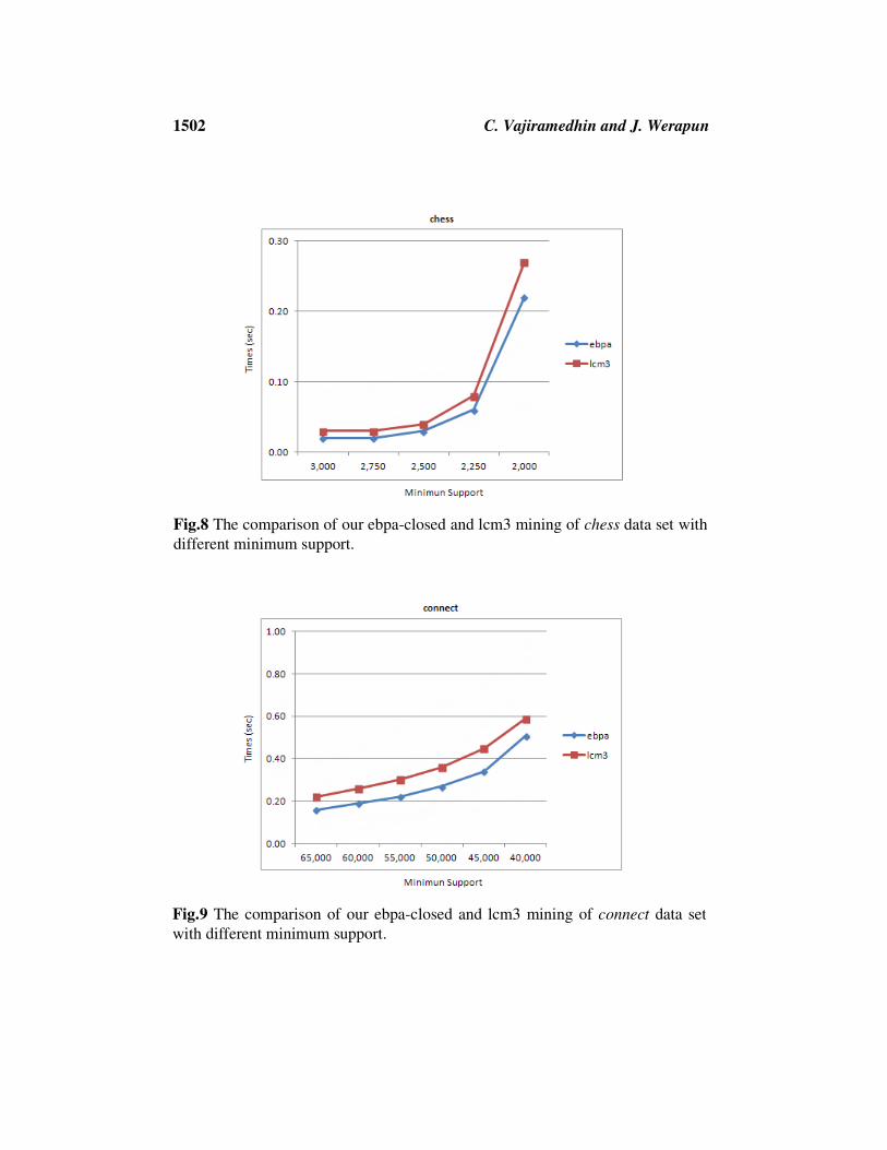
Fig.8 The comparison of our ebpa-closed and lcm3 mining of chess data set with

different minimum support.

Fig.9 The comparison of our ebpa-closed and lcm3 mining of connect data set

with different minimum support.


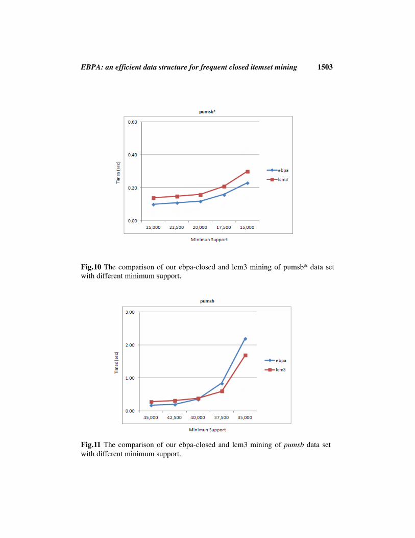
Fig.10 The comparison of our ebpa-closed and lcm3 mining of pumsb* data set


Fig.11 The comparison of our ebpa-closed and lcm3 mining of pumsb data set



The results showed that our ebpa approach performed very well on three

datasets (chess, connect, pumsb*), which outperformed over those of the lcm3

approach. However, the percentage of improved results also depended on each

type of datasets such as improved up to 22% on chess, 15% on connect, and 30%

on pumsb* respectively. In all datasets, when decreasing the minimum support

values (in the dataset), the response time increased in both approaches (ebpa,

lcm3) because of the less minimum support values, the more frequent 1-itemsets

and more time needed to process. For three of four datasets, our ebpa

outperformed over those of the lcm3. The reason is that we introduce the

improved collaboration data structure that provides the efficient FCIM mining, as

illustrated in their time complexity (in Section 3.2 and 3.3). Time complexity of

the FCIM algorithm (i.e., time for creating the initial data plus time for processing

FCIM) in the lcm3 (using the original collaboration data structure [10]) is [O(mT)

+ O(mniT’)] + O(m2n), where as that of our EBPA-based FCIM algorithm is

[O(m2n) + O(mT)] + O(m

2n). Cleary, the response time of constructing our

(compact) prefix tree is improved over that of the existing collaboration if the

unique transactions (T’) are more than the number of occurrence nodes (n)

because (in practice) most of transaction databases and available datasets

composts of T’ > n. However, when n > T’ (in some datasets i.e., pumsb for

min_supp < 40000 (Fig.11)), which there exist a lot of repeated transactions (less

T’) and a variety of itemsets (more n), the response time of the lcm3 is less than

our ebpa approach.

5 Conclusion

This paper presents an improved collaboration data structure, called the EBPA

data structure, and its corresponding algorithm (the EBPA-CLOSED algorithm)

for frequent closed itemset mining (FCIM). Our proposed EBPA (Efficient

Bitmap Prefix-tree Array) data structure for efficient FCIM algorithm can

improve both space and time with O(1) parent-child access (into the prefix-tree

array). The performance evaluation was performed on four available datasets,

which were pumsb, pumsb*, chess, and connect. Experimental results showed that

our EBPA-based closed itemset mining (ebpa) can reduce response time up to

15-30% over that of the lcm3 in pumsb*, chess and connect datasets. Finally, our

future research will focus on designing an efficient parallel EBPA-CLOSED

algorithm with the EBPA data structure on multi-core systems.

Acknowledgement

We would like to thank the Office of the Higher Education Commission of

Thailand and Ubonratchathani University for the financial support. We are also

grateful to the owner of the datasets for providing the available datasets and the

LCM editors for posting the best programming code.


References

[1] N. Pasquier, Y. Bastide, R. Touil and L. Lakhal, Discovering frequent closed

itemsets for association rules, Proceedings of 7th International Conference on

Database Theory (ICDT 1999), LNCS, vol.1540, Springer-Verlag,

Jerusalem, Israel, 1999.

[2] N. Pasquier, Y. Bastide, R. Taouil and L. Lakhal, Efficient Mining of

Association Rules Using Closed Itemset Lattices, Information Systems, vol.

24, no. 1, 1999, 25-46.

[3] J. Pei, J. Han and R. Mao, CLOSET: An Efficient Algorithm for Mining

Frequent Closed Itemsets, Proceedings of ACM SIGMOD Int’l Workshop

Data Mining and Knowledge Discovery, 2000.

[4] M.J. Zaki and C.-J. Hsiao, CHARM: An Efficient Algorithm for Closed

Itemsets Mining, Proceedings of Second SIAM Int’l Conf. Data Mining,

2002.

[5] G. Grahne and J. Zhu, Efficiently Using Prefix-Trees in Mining Frequent

Itemsets, Proceedings of ICDM Workshop Frequent Itemset Mining

Implementations, 2003.

[6] J. Pei, J. Han and J. Wang, CLOSET+: Searching for the Best Strategies for

Mining Frequent Closed Itemsets, Proceedings of Ninth ACM SIGKDD Int’l

Conf. Knowledge Discovery and Data Mining, 2003.

[7] T. Uno, T. Asai, Y. Uchida and H. Arimura, LCM: An Efficient Algorithm

for Enumerating Frequent Closed Item Sets, Proceedings of IEEE ICDM’03

Workshop FIMI’03, 2003.

[8] T. Uno, M. Kiyomi and H. Arimura, LCM ver.2: Efficient Mining Algorithm

for Frequent Closed Maximal Itemsets, Proceedings of IEEE ICDM’04

Workshop FIMI’04, 2004.

[9] C. Lucchesse, S. Orlando and R. Perego, DCI-Closed: a fast and memory

efficient algorithm to mine frequent closed itemsets, Proceedings of the IEEE

ICDM Workshop on Frequent Itemset Mining Implementations (FIMI’04),

volume 126 of CEUR Workshop Proceedings, Brighton, UK, 2004.

[10] T. Uno, M. Kiyomi and H. Arimura, LCM ver.3: Collaboration of Array,

Bitmap and Prefix Tree for Frequent Itemset Mining, Proceedings of Open

Source Data Mining Workshop on Frequent Pattern Mining Implementations

2005, 2005.

[11] T. Uno, T. Asai, Y. Uchida and H. Arimura, An Efficient Algorithm for

Enumerating Closed Patterns in Transaction Databases, IEEE ICDM

workshop FIMI’04, Zaki & Goethals, 2004.

[12] C. Lucchese, S. Orlando and R. Perego, Fast and Memory Efficient Mining

of Frequent Closed Itemsets, IEEE Transactions on Knowledge and Data

Engineering, vol. 18, no. 1, 2006, 21-36. [13] J. Sribuaban, V. Boonjing and J.Werapun, Frequent Closed Multi

dimensional Multi-level pattern mining, Proceedings of the Fourth IASTED

International Conference on Advances in Computer Science and Technology,

Malaysia, 2008, 201-206.


[14] J.Wachiramethin and J.Werapun, BPA: A Bitmap-Prefix-tree Aarray data

structure for frequent closed pattern mining, Proceedings of the Eighth

International Conference on Machine Learning and Cybernetics, Baoding,

China, 2009, 154-160.

Received: January, 2013

ebpa: an efficient data structure for frequent closed itemset mining

Documents