ece 487 lecture 3 : foundations of quantum mechanics...

ECE 487Lecture 5 : Foundations of

Quantum Mechanics IV

Class Outline:

•Linearly Varying Potential•Triangular Potential Well•Time-Dependent Schrödinger Equation

• How do the solutions to Schrödinger’s equation change when there is a field and well is finite on one side?

• How do the solutions to Schrödinger’s equation change when there is a field and well is finite on both sides?

• How can we think about solving the Schrödinger equation for time dependent situations?

M. J. Gilbert ECE 487 – Lecture 5 02/01 /1 1

Things you should know when you leave…

Key Questions


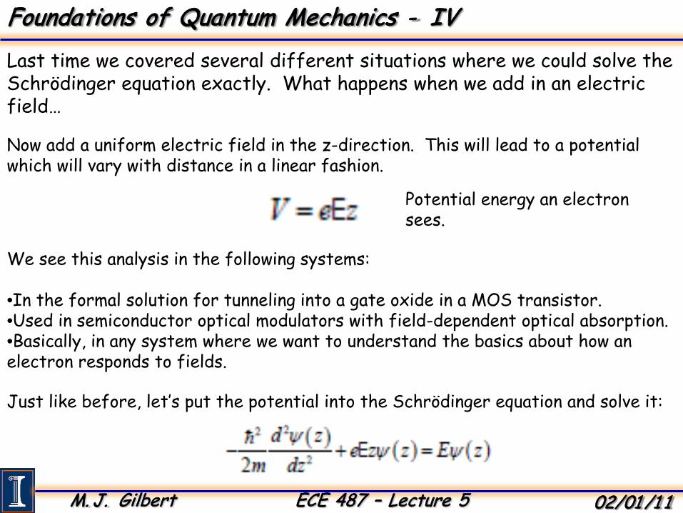
Last time we covered several different situations where we could solve the Schrödinger equation exactly. What happens when we add in an electric field…

Foundations of Quantum Mechanics - IV

Now add a uniform electric field in the z-direction. This will lead to a potential which will vary with distance in a linear fashion.

Potential energy an electron sees.

We see this analysis in the following systems:

•In the formal solution for tunneling into a gate oxide in a MOS transistor.•Used in semiconductor optical modulators with field-dependent optical absorption.•Basically, in any system where we want to understand the basics about how an electron responds to fields.

Just like before, let’s put the potential into the Schrödinger equation and solve it:


The solution to the Schrödinger equation this time is comprised of another strange function, the Airy function…


The standard form of the differential equation which defines the Airy functions is:

The solutions are formally the Airy functions Ai(ζ) and Bi(ζ):

But to get to this point, we had to make a substitution into our original equation using a change of variables:

using


So what do the Airy functions look like?


•Both functions are oscillatory for negative arguments with shorter and shorter period as the functions become more negative.

•The Ai function decays in an exponential fashion for positive arguments.

•The Bi function diverges for positive arguments.


So let’s consider a situation where the potential varies linearly without any boundaries…


•Here there are two possible solutions: one based on the Ai and one based on the Bi.•But we can discard the Bi solutions because the diverge for positive values.•Therefore, we are only left with the Ai solutions.

Now put it back into our solution with the correction for the change in variables and we now have the form of the eigenfunctions in our linearly varying potential.


More interesting things to note:


•There are mathematical solutions for any possible value of the eigenenergywhich reminds us of having no potential anywhere.

•This leads to plane wave solutions for any positive energy.

•The allowed eigenvalues are continuous and not discrete.

•The solution is oscillatory when the eigenenergy is greater than the potential energy and decays when the eigenenergy is less than the potential energy.

•The eigenfunction solutions for different energies are the same except they are shifted sideways in position.

•Unlike the solutions to the uniform potential, these solutions are not traveling waves but rather standing waves like in quantum wells.

•Again we have stable eigenstates because we are not considering the time dependence.


But how can we even rationalize standing waves in this case?


•We can rationalize this by assuming that the particle is bouncing off of the increasing potential.

•This is why we see a reflection at the right.

•There is any reflection on the left because any change in potential leads to reflections.

•The fact that there are distributed reflections explains why the wave amplitude decreases progressively as we go to the left.

•The fact that we have a standing wave is apparent because integrated in energy the reflection will eventually total 100%.


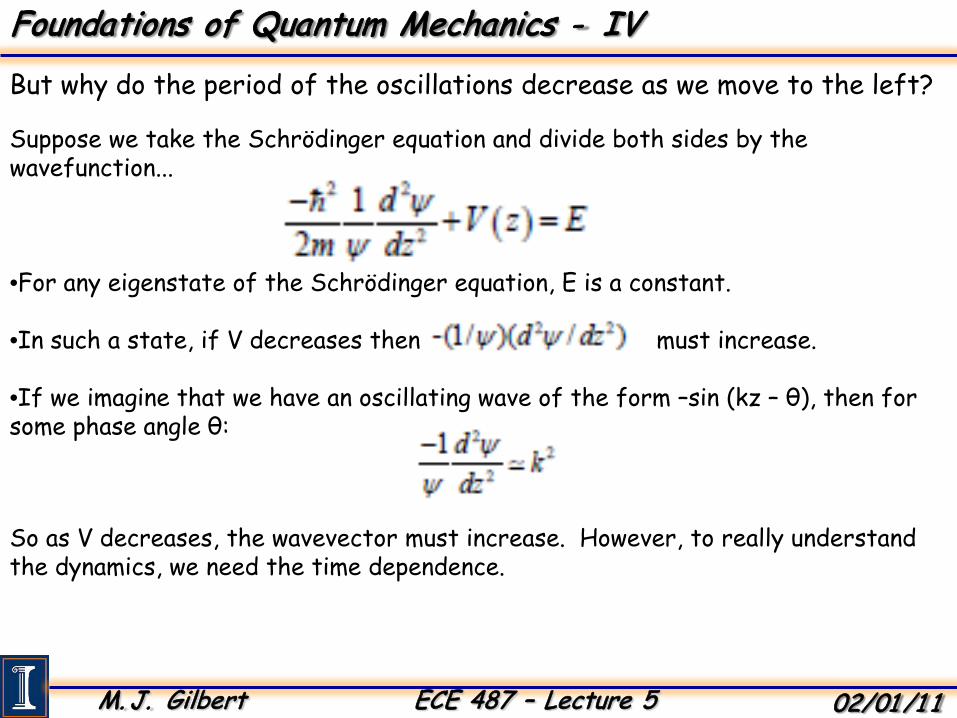
But why do the period of the oscillations decrease as we move to the left?


Suppose we take the Schrödinger equation and divide both sides by the wavefunction...

•For any eigenstate of the Schrödinger equation, E is a constant.

•In such a state, if V decreases then must increase.

•If we imagine that we have an oscillating wave of the form –sin (kz – θ), then for some phase angle θ:

So as V decreases, the wavevector must increase. However, to really understand the dynamics, we need the time dependence.


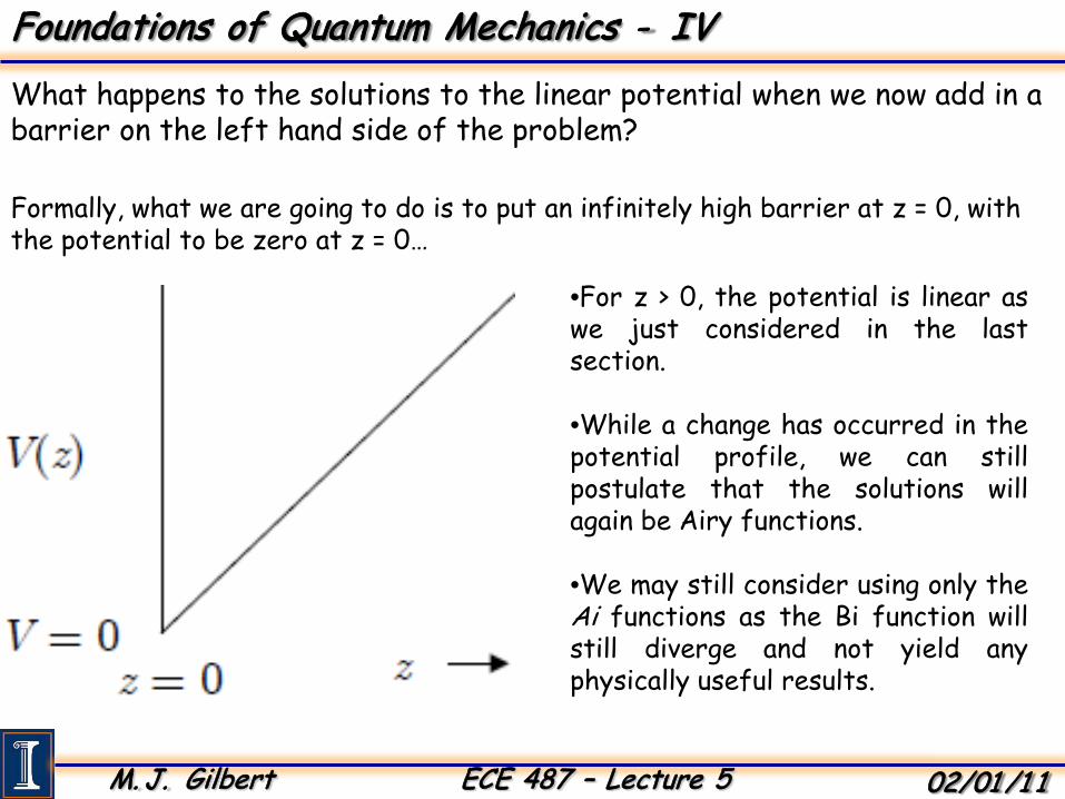
What happens to the solutions to the linear potential when we now add in a barrier on the left hand side of the problem?


Formally, what we are going to do is to put an infinitely high barrier at z = 0, with the potential to be zero at z = 0…

•For z > 0, the potential is linear aswe just considered in the lastsection.

•While a change has occurred in thepotential profile, we can stillpostulate that the solutions willagain be Airy functions.

•We may still consider using only theAi functions as the Bi function willstill diverge and not yield anyphysically useful results.


But we still have to account for the change in boundary conditions at z = 0…


•This means that the wavefunction will have to go to zero at z = 0.

•This condition is easily satisfied with the Ai function if we position it laterally so that one of the zeros is found at z = 0.

•The Ai(ζ) function will have zeros for a set of values ζi.

The first few zeros we list here:

Plot of the wavefunctions andenergy levels in a triangularpotential well we E = 1 V/Å


But now we have to change the way we look at the wavefunctions, Ai, because we need make sure the boundary conditions are met…


In other words, we need to get the wavefunction:

To be zero at z = 0, or

The argument of the Ai function must be one of the zeros.

Equivalently, we could also lookat the energy eigenvaluespectrum…


What happens if we take the infinite potential well and add in the linearly varying potential?


•This is formally equivalent to taking the problem of the electron in a triangular well with the additional boundary condition on the other side at z = Lz.

•Now we can no longer simply assume that we can get rid of the Bi solutions.

•The potential forces the wavefunction to go to zero at the right wall as well as the left wall so there will be no wavefunction amplitude to the left or the right.

•The divergence in Bi no longer matters for normalization as we are normalizing only inside the box..

Now we need the full solution:


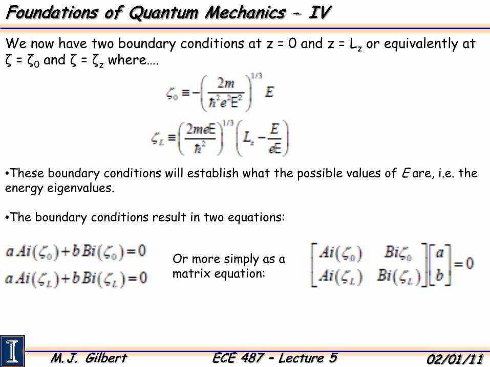
We now have two boundary conditions at z = 0 and z = Lz or equivalently at ζ = ζ0 and ζ = ζz where….


•These boundary conditions will establish what the possible values of E are, i.e. the energy eigenvalues.

•The boundary conditions result in two equations:

Or more simply as amatrix equation:


The usual condition for the solution to such an equation would be the following:


equivalently

Now we need to find which values of ζL satisfy the above equation. This looks like a problem which is set up to be solved on a computer…

•Before we solve it numerically, we can simplify some of the notation by making some substitutions which change things into dimensionless units.

•There are two relevant energies:

1. the natural unit for discussing potential well energies – the energy of the lowest state in an infinitely deep potential well:

We just call it to avoid confusion with the solutions of this problem.

∞1E


So now let’s define the dimensionless “energy” for our problem:


2. The second energy in the problem is the potential drop from one side of the well to the other which results from the electric field

Get rid of dimensions

Now we can rewrite our zeta terms using these new dimensionless units:


Now choose a vL corresponding to the electric field which has been applied across the infinite quantum well of a given width.


For example, say we have a 6 Å quantum well with a field of 1 V/Å. Then…

As we did in the triangular quantum well, we seek the solutions which make the determinant of the matrix equation equal to zero…

•To accomplish this we graph this function from ε = 0 upwards to find the approximate position of the zero crossings, then find the roots…

•With the eigenvalues we can evaluate the wavefunctions of the general solution for each eigenenergy:


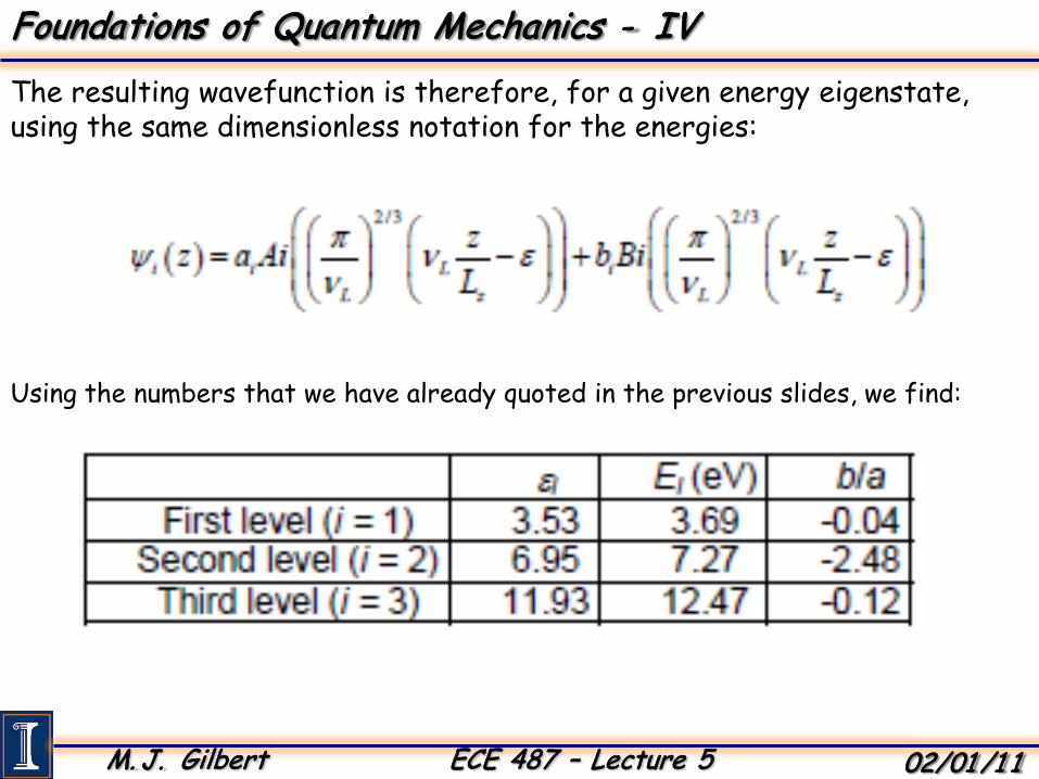
The resulting wavefunction is therefore, for a given energy eigenstate, using the same dimensionless notation for the energies:


Using the numbers that we have already quoted in the previous slides, we find:


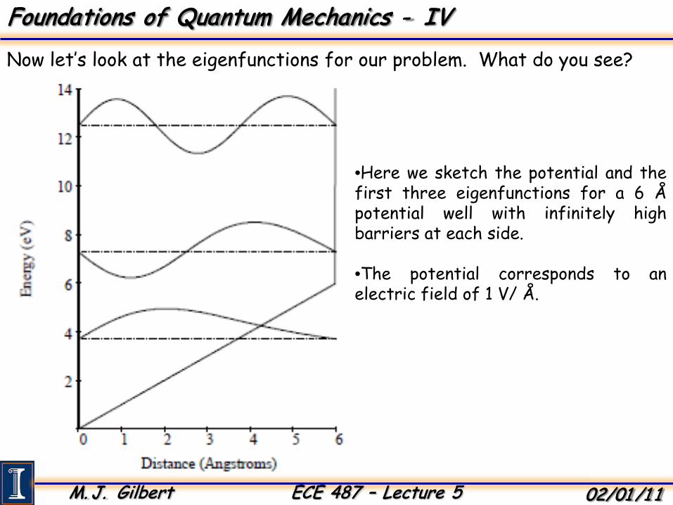
Now let’s look at the eigenfunctions for our problem. What do you see?


•Here we sketch the potential and thefirst three eigenfunctions for a 6 Åpotential well with infinitely highbarriers at each side.

•The potential corresponds to anelectric field of 1 V/ Å.


We should notice…


•All of the wavefunctions go to zero at the sides of the well.

•This is required by the boundary conditions.

•The lowest solution is almost identical in energy to that of the lowest state in the triangular well.

•This is because the fraction of the Bi Airy function is very small, ~ 0.04.

•The energy is slightly higher than the normal triangular well because the system is more confined.


Anything else?


•The second solution is now very strongly influenced by the potential barrier at the right.

•However, it is at a much higher energy that in the triangular well.

•The third solution is very close in form to that of the infinite square quantum well.

•Looks pretty sinusoidal but the period is shorter on the left hand side.

•Why?


Finally…


•In the lowest state, the electron is pulled closer to the left hand side but we would expect this even classically.

•But the classical intuition we used for the first level doesn’t work at all for the second level.

•Calculate the probability density and we find that the electron has a 64% chance to be found on the left of the well and only a 36% chance of being found on the right hand side.


Thus far we have assumed that most things were steady in time, but that was pretty unsatisfying because intuitively we know the solution contains motion with time evolution…


Consider several situations we have already encountered:

1. Simple harmonic oscillator2. Electrons in an electric field

So to understand these things we need to keep the time dependence in the Schrödinger equation.

•But remember this is still very different from the normal classical time dependent wave equation.

•To solve this problem, we need to introduce a very important concept in quantum mechanics, superposition states.

•These states allow us to handle the time evolution in quantum mechanics very easily.


The key to understanding the time dependence and the Schrödinger equation is understanding the relationship between frequency and energy in quantum mechanics…


A good example of this is the case of electromagnetic waves and photons. Imagine two experiments with a monochromatic electromagnetic wave.

•In one experiment, we measure the frequency of the oscillation in the wave.

•In a second experiment, we count the number of photons per second.

So, we can count how many photons per second correspond to a particular power at this frequency…

However, this discussion is for photons and these particles are not well described by the Schrödinger equation.


But there is a problem…


+q

-q

( ) 220

40 6.13

42 neV

nqmEH −==πε

n = 1, 2, 3, …

•Hydrogen atoms emit photons as theytransition between energy levels.

•We expect some oscillation in theelectrons at the corresponding frequencyduring the emission of the photon.

•So we should also expect a similar relationbetween energy and frequency associatedwith the electron levels.

ece 487 lecture 3 : foundations of quantum mechanics...

Documents