1

ECE 487: Final Report

Design and Calibration of a Raman Spectrometer for use in a Laser

Spectroscopy Instrument Intended to Analyze Martian Surface and

Atmospheric Characteristics for NASA

Authors:

John F. Lucas (EE)

James Hornef (EE)

486 Group:

Derek Davis

Faculty Adviser:

Dr. Hani Elsayed-Ali

NASA Adviser:

Dr. M Nurul Abedin

Old Dominion University

Department of Electrical and Computer Engineering

April 18th 2016

2

Abstract

This project’s goal is the design of a Raman spectroscopy instrument to be utilized by NASA in

an integrated spectroscopy strategy that will include Laser-Induced Breakdown Spectroscopy (LIBS) and

Laser-Induced Florescence Spectroscopy (LIFS) for molecule and element identification on Mars Europa,

and various asteroids. The instrument is to be down scaled from a dedicated rover mounted instrument

into a compact unit with the same capabilities and accuracy as the larger instrument. The focus for this

design is a spectrometer that utilizes Raman spectroscopy. The spectrometer has a calculated range of 218

nm wavelength spectrum with a resolution of 1.23 nm. To filter out the laser source wavelength of 532

nm the spectrometer design utilizes a 532 nm wavelength dichroic mirror and a 532 nm wavelength notch

filter. The remaining scatter signal is concentrated by a 20 x microscopic objective through a 25-micron

vertical slit into a 5mm diameter, 1cm focal length double concave focusing lens. The light is then

diffracted by a 1600 Lines per Millimeter (L/mm) dual holographic transmission grating. This spectrum

signal is captured by a 1-inch diameter double convex 3 cm focal length capture lens. An Intensified

Charge Couple Device (ICCD) is placed within the initial focal cone of the capture lens and the Raman

signal captured is to be analyzed through spectroscopy imaging software. This combination allows for

accurate Raman spectroscopy to be achieved. The components for the spectrometer have been bench

tested in a series of prototype developments based on theoretical calculations, alignment, and scaling

strategies. The mounting platform is 2.5 cm wide by 8.8 cm long by 7 cm height. This platform has been

tested and calibrated with various sources such as a neon light source and ruby crystal. This platform is

intended to be enclosed in a ruggedized enclosure for mounting on a rover platform. The size and

functionality of the Raman spectrometer allows for the rover to carry other mission critical devices. This

project will be continued at NASA until the requirements are met for the expected initial 2020 launch

date.

3

1 CONTENTS

2 Introduction ........................................................................................................................................... 5

3 Theory ................................................................................................................................................... 6

3.1 Raman Spectroscopy ..................................................................................................................... 6

3.2 Spectrometer ................................................................................................................................. 7

4 Current Design ...................................................................................................................................... 9

4.1 System Arrangement ..................................................................................................................... 9

4.1.1 532 nm Laser (A) .................................................................................................................. 9

4.1.2 532 nm dichroic mirror (B): .................................................................................................. 9

4.1.3 Target material (C): ............................................................................................................... 9

4.1.4 532 nm wavelength notch filter (D): ..................................................................................... 9

4.1.5 20 x Microscopic objective (E): ............................................................................................ 9

4.1.6 25 micron Slit (F): ................................................................................................................. 9

4.1.7 Focusing Lens (G):................................................................................................................ 9

4.1.8 Dual Holographic Grating (H) .............................................................................................. 9

4.1.9 Capture Lens (I) .................................................................................................................. 10

4.1.10 ICCD Camera (J): ............................................................................................................... 10

4.2 Design Constraints ...................................................................................................................... 11

4.3 Calibration and Results ............................................................................................................... 12

4.4 Alternate Design ......................................................................................................................... 14

4.4.1 Alternate Design 1 .............................................................................................................. 14

4.4.2 Alternate Design 2 .............................................................................................................. 16

5 Realistic Constraints ........................................................................................................................... 18

6 Impacts of the Design ......................................................................................................................... 21

6.1 Economic .................................................................................................................................... 21

6.2 Environmental ............................................................................................................................. 21

6.3 Health & Safety ........................................................................................................................... 21

6.4 Contemporary Issues ................................................................................................................... 21

7 Lifelong Learning ............................................................................................................................... 22

7.1 Knowledge from Other Courses ................................................................................................. 22

7.1.1 James Hornef ...................................................................................................................... 22

7.1.2 John F. Lucas (Jay) ............................................................................................................. 22

4

8 Engineering Standards ........................................................................................................................ 23

9 Conclusion .......................................................................................................................................... 24

10 References ....................................................................................................................................... 24

11 Appendix A: Meeting Log .............................................................................................................. 26

5

2 INTRODUCTION

As humans reach out to explore our solar system, various obstacles stand in the way. Time and money

are main concerns with any human endeavor. There are other naturally occurring obstacles that are inherit

to space travel and planet atmosphere entry. Human curiosity, creativity, and perseverance push us to

overcome these obstacles. The planets within our solar system remain largely a mystery past a cursive

understanding. Since the first satellite sent to space, Sputnik 1, on October 4, 1957 [1], the human race

has been pushing the innovation of technology that could be used to explore outer space and one day

reach the planets of our solar system. The technology used for exploration has evolved from computers

that are less powerful than a smart phone into semi-autonomous rovers that can acquire data without the

need of sending humans to space. These rovers are equipped with a vast amount of technology that allows

for the analysis of newly encountered environments. Equipment such as solar panels, temperature sensors,

and spectrometers are basic components for exploratory rovers. Each piece of equipment is required to be

of the highest quality and durability while simultaneously being as compact, accurate, and efficient as

possible. The less area and weight each piece equipment takes up on a rover platform the less cost it is to

transport into space.

As exploration of our solar system continues and grows it is necessary to gain information in an

efficient and precise manner. This project is tasked with providing an accurate sensor for detecting and

discerning a variety of material. The data gathered by this instrument will be used to identify surface

materials of various planetary and asteroid environments with the focus of this version of the design being

deployment on Mars.

This project provides a small scale Raman spectrometer for the proposed areas of Earth’s solar system

exploration. The capabilities of the Raman spectrometer will be integrated, by a different group, with a

larger platform that will eventually be used for matter detection and identification. The conglomerate

system is based on Raman, LIF, and LIBS spectroscopy integrated with LIDAR. The system will be less

than 5 kg in weight and fits within the following dimensions: 25.40 cm x 25.40 cm x 20.32 cm. This

device will be able to analyze a sample by collecting data via LIF, LIBS, Raman, and LIDAR and will be

able to store the data readings on an internal memory card. Power will be supplied through an external

source to the system. It is desired for this instrument to be a multi-platform instrument with the first

incarnations catered for rover mounting and autonomous triggering.

The specific area of this project is the design, scaling, and calibration of an accurate Raman

spectroscopy instrument. It is mission critical to provide an accurate spectrometer within a relatively

small scale footprint. The existing large scaled system, which includes LIF, LIBS, and Raman

spectroscopy, has a range of 300 nm that is expanded to 600 nm by using a dual holographic grating

strategy [5]. This project uses a single transmission dual holographic grating with Raman spectroscopy

techniques. The spectrometer developed for this project currently has a footprint of 3.5 cm wide by 7.9

cm long with a wavelength range of 218 nm at a resolution factor of 1.23. This exceeds the range of 200

nm while keeping the resolution factor less than 2 as per the proficiencies set forth in the proposal for this

project. The Raman spectrometer has been designed and scaled using a series of theoretical calculations

and experiments that are described in this paper. The capabilities described allow for a variety of accurate

material detection in keeping with the abilities of the original larger scaled system. This has been

accomplished by a series of configurations and calibrations in comparison with the large scale existing

system and within the size and abilities constraints set for this project.

6

3 THEORY

3.1 RAMAN SPECTROSCOPY Raman spectroscopy is a powerful tool that provides information about molecular vibrations that

can be used for sample identification and quantitation [2]. When a laser light is shined on a sample, the

photons of the laser light are absorbed by the sample and the reemitted. The frequency of the reemitted

photons is shifted up or down in comparison with the original frequency, which is better known as the

Raman Effect [3]. This shift is then used to identify the molecules based on their Raman shift frequency.

In simplistic terms, Raman scattering uses the vibrational energies to identify the chemical composition of

a material. An example of a Raman Scattering spectrum is shown in Figure 1[4]. In the case of Dr.

Abedin’s recent publication [5], the Raman shift was performed with a 532 nm wavelength laser. This

wavelength is chosen based on the impact that it has the experimental capabilities. These impacts include

sensitivity, spatial resolution, and optimization of the wavelength.

Figure 1: Example of Raman Scattering Spectrum [4]

Raman scattering is primarily used to identify pure elements, simple molecules, and

organic/inorganic materials. Within the detection of organic materials, Raman scattering can distinguish

specific compounds such as lipids, amino acids and even nucleic acids (DNA)- [6]. This makes Raman

scattering a powerful tool for identifying simple molecules and organic materials. Despite this amazing

analysis ability, Raman Scattering has a major downside. Raman Scattering cannot identify metals or

alloys and it cannot identify molecules with ionic bonds. This is because these types of materials are more

difficult to identify the vibrational characteristics. In short, Raman scattering cannot identify a compound

that it cannot vibrated easily.

7

3.2 SPECTROMETER Diffraction gratings are used to disperse light, meaning that it separates light into different

wavelengths [7]. These gratings have replaced prisms as primary sources of spectral analysis due to their

unique ability to control the spectral wavelength and spectral range to a certain degree. This is done by

using two parameters; the groove density and the blaze angle [8]. The groove density is the amount of

grooves there is on the grating per millimeter and the blaze angle is the angle at which the grating is most

effective at dispersing light. For this project, the grating being used is a dual holographic grating with a

blaze angle for 532 nm and a groove density of 1600 grooves/mm.

The groove density determines the spectrometer’s wavelength coverage and is a major factor in

determining the spectral resolution of the system [9]. The wavelength coverage of the spectrometer is

inversely proportional to the dispersion of the grating due to its fixed geometry. This means that the

greater the dispersion factor, the greater the resolving power of the spectrometer. Knowing this, it

becomes clear that as the wavelength coverage increases, the spectral resolution decreases. For a fixed

grating spectrometer, the angular dispersion from the grating is described by the following equation:

𝑑𝛽

𝑑𝜆=

𝑚

106𝑑𝑐𝑜𝑠(𝛽)

Where 𝛽 iss the diffraction angle, d is the groove period (also known as the inverse of the groove

density), m is the diffraction order of the light and 𝜆 is the wavelength of light as shown in Figure 2.

Figure 2: Wavelength of light in reference to the grating.

When the focal length (F) is taken into account and by assuming the small angle approximation,

the equation can be generated to provide the linear dispersion in terms of nm/mm. The following equation

shows this alteration:

𝑑𝜆

𝑑𝐿=106𝑑𝑐𝑜𝑠(𝛽)

𝑚𝐹

From this linear dispersion equation, the maximum spectral range, (𝜆𝑀𝐴𝑋 − 𝜆𝑀𝐼𝑁), can be

calculated based on the detector length (𝐿𝐷). The detector length is found by multiplying the number of

pixels on the detector (𝑛) by the width of the pixel (𝑊𝑝). The resulting equation is shown below:

(𝜆𝑀𝐴𝑋 − 𝜆𝑀𝐼𝑁) = 𝐿𝐷𝑑𝜆

𝑑𝐿= 𝐿𝐷 (

106𝑑𝑐𝑜𝑠(𝛽)

𝑚𝐹)

8

Another important characteristic of a spectrometer is the spectral resolution. This parameter

determines the maximum number of spectral peaks that a spectrometer can resolve. For example, if a

spectral range of a spectrometer is 200 nm and it has a spectral resolution of 1 nm, the system would be

able to resolve a maximum of 200 individual peaks across the spectrum. There are three main factors that

determine this spectral resolution: the slit, the diffraction grating, and the detector. The slit determines the

minimum image size that the can be formed on the detector plane. The diffraction grating determines the

total wavelength range of the spectrometer. And the detector determines the maximum number and size of

discreet points in which the spectrum can be digitally analyzed.

When calculating the spectral resolution (𝛿𝜆) of a spectrometer, there are four parameters that

need to be known. These parameters are the slit width (𝑊𝑆), the spectral range (𝜆𝑀𝐴𝑋 − 𝜆𝑀𝐼𝑁), the pixel

width (𝑊𝑃) and the number of pixels in the detector (n). Another important factor to know is the

resolution factor (RF). This value is determined by the relationship between the slit width and the pixel

width. This is important because the spectral resolution is not the only factor in determining the observed

signal from the spectrometer. This reading is also dependent on the linewidth of the signal but this signal

is normally assumed to be so narrow that it can be neglected in the equation. To ensure that this condition

is met, it is important to ensure that the linewidth is significantly narrow. This is accomplished by

collecting data from a low pressure lamp, like Hg vapor, since the linewidth of these sources are typically

much narrower than the spectral resolution. Once this data is collected, the spectral resolution is measured

at the full width half maximum of the peak of interest. This value takes a minimum of 3 pixels to read this

value and this means that the spectral resolution, assuming that 𝑊𝑆 = 𝑊𝑃, is equal to three times the pixel

resolution.

The resolution factor is equal to 3 when 𝑊𝑆 ≈ 𝑊𝑃 due to this fact. When 𝑊𝑆 ≈ 2𝑊𝑃, the

resolution factor drops to 2.5. This value continues to drop until 𝑊𝑆 > 4𝑊𝑃, when the resolution factor

levels out to 1.5. All of these parameters can be combined to create the following equation:

𝛿𝜆 =𝑅𝐹 ∗ ∆𝜆 ∗𝑊𝑠

𝑛 ∗𝑊𝑝

The diffracting gradient is a 1600 grooves per micron dual holographic transmission grating with a

blaze angle that makes 532 nm wavelength the optimal wavelength. The diffracting gradient allows the

light to diffract into the wavelengths that are present in the remaining scatter. The diffracted light then hits

a capturing lens and is transmitted into the ICCD camera.

9

4 CURRENT DESIGN

4.1 SYSTEM ARRANGEMENT The system arrangement out of the system is shown in Figure 3 page 9.

4.1.1 532 nm Laser (A)

Nd: YAG (neodymium-doped yttrium aluminum garnet; Nd: Y3Al5O12) diode pumped, Q-

switched 500 mW Laser. The pulse rate was set to 1 kHz.

4.1.2 532 nm dichroic mirror (B):

This dichroic mirror acts as a targeting mirror for the laser beam. The 532 nm laser beam hits this

dichroic mirror at 45 degrees and is reflected to the target. The laser will hit the material and a

Raman signal plus the reflected 532 signal will come back to the dichroic mirror. The 532 nm

signal is filtered out by the dichroic mirror and the shifted Raman signal is allowed to pass

through. The 532 nm laser signal would not only give false material results but would damage the

Intensified Charge Coupled Device (ICCD).

4.1.3 Target material (C):

Neon light source, ruby crystal and naphthalene will be used during data gathering.

4.1.4 532 nm wavelength notch filter (D):

The second filter is necessary to reassure that all of the 532 nm wavelength source laser signal is

filtered from the system. This insures that there will be no damage to the ICCD camera from this

signal. The notch filter transmits 80% of 350 to 400 nm, 93% of 400 m to 513.2 nm, and 93% of

550.8 nm to1600 nm.

4.1.5 20 x Microscopic objective (E):

The microscopic objective intensifies the captured return signal into the micro slit. This will allow

for a weaker signal to have enough gain to produce a signal that is absent feedback.

4.1.6 25 micron Slit (F):

The 25 micron slit collimates the light for transmission to the focusing lens. 50 and 100 micron

slits are also used to give the optimal signal pass through versus collimation. If the signal is weak,

the 50 or 100 micron slit can be used to allow a stronger signal.

4.1.7 Focusing Lens (G):

This lens is a double convex lens with a 5 mm diameter with a focal length of 1 cm. The lens

focuses the light signal from the slit onto the grating. The reason for having a focused light spot

area on the diffraction grating is to capture as much signal as possible so that when the signal is

diffracted into a spectrum there is still a comparatively strong signal to gather Raman shift data.

4.1.8 Dual Holographic Grating (H)

The dual holographic grating is a transmission grating with 1600 lines per mm. The angle of

incidence is 45° and the angle of transmission is 45°. The dual holographic grating angle of

placement and lines per millimeter number are key elements to the spectrometer. The angle

allows for optimal placement within the spectrometer to allow for a smaller footprint. The focal

length is also important to the footprint of the spectrometer as the size is a key constraint to this

10

project. The lines per millimeter of the grating determine the range developed in the spectrum.

The more lines the higher the wider range of the spectrum. This grating also creates two

spectrums that are staggered on top of each other. This allows more of the spectrum to be

captured while using a smaller sized capture lens and ICCD.

4.1.9 Capture Lens (I)

The capture lens is a 1 cm diameter, AR (anti-reflective) coated lens that has a focal length of 3

cm. The purpose of the AR coating is to prevent the internal reflection of the signal within the

lens. The capture lens captures and focuses the transmitted spectrum from the grating. The reason

for the second capture lens being larger than the first is to ensure that as much of transmitted

spectrum is captured as possible.

4.1.10 ICCD Camera (J):

The ICCD Camera type is sensitive information. The resolution is 6.45-micron pixel width 2048 x

2048 number of pixels and a 1.2 nm resolution.

Figure 3: Spectrometer arrangement in relation to external components and target material.

11

4.2 DESIGN CONSTRAINTS The dichroic mirror and the notch filter, screen 532 nm wavelength due to the wavelength of the

excitation laser (See Figure 3; Elements A, B, and D; Page 10). The notch filter sits parallel to the

dichroic mirror, which must be at 45° incidence angle to the excitation laser. The redundant notch filters

ensure that any bleed through 532 nm wavelength will be removed from the scatter and that the analysis

will be accomplished without interference from the source excitation laser beam (See Figure 3; Page 10).

The 20x microscope objective concentrates the remaining scatter into a 25-micron slit (See Figure

3; Elements E and F; Page 10). The slit can be changed alternatively to a 50-micron and 100-micron size

as to allow for a stronger signal to pass through during the calibration process.

The focus lens has a 1 cm focal length, which constrains the position of the lens to grating. The

capture lens has a focal length of 3 cm. In order for optimal Raman signal reading the ICCD must be

positioned as close to the focal length of the capture lens as possible. (See Figure 3; Elements G, I, and J;

Page 10).

The dual holographic transmission grating (See Figure 3; Element H; Page 10) diffracts the light

into a spectrum with the spectrum range based on the 1600 lines (grooves) per millimeter (lpmm) of the

grating and the matching systems angle matching to the grating incidence and transmission angles.

Spectral wavelength and spectral range are controlled using two parameters; the groove density and the

blaze angle.

The current design has a range of 218 nm wavelength with a 1.23 resolution. The total size is 2.8 cm

wide by 8.3 cm long by 7 cm height (See Figure 4).

Figure 4: Current design arrangement 4/18/16.

12

4.3 CALIBRATION AND RESULTS A visual calibration has been accomplished without an ICCD camera. However, the visual

calibration will not be sufficient for the collection of reliable data. The ICCD will collect and transmit

precise data to that will be analyzed through a spectrometer imaging program. Visual calibration that were

used were measured optically, i.e. what could be visibly be seen on the target. Visual calibration has been

accomplished by measurement of spectrum width from white light source and neon source (See Figure 5).

A white light source was aimed into the spectrometer and the spectrum was observed and marked on a

white paper target. The spectrum was measured at approximately 4mm or 400 nm. The spectrometer

optics were aligned using a 629 nm wavelength 500mW laser. This laser was also observed on a target

blank white sheet of paper. The laser appears to fall within the expected range in a red color of

approximately 629 nm wavelength. Lastly for a neon source was aimed into the spectrometer. The neon

light was observed to fall within the expected visible light wavelength range for yellow to orange.

Figure 5: In order from top to bottom: An illustration of a visible light spectrum, White light source

spectrum and a Neon source.

After the spectrometer was aligned optically, the ICCD camera replaced the white sheet of paper.

Since the ICCD is very sensitive to external light, the entire spectrometer had to be covered by a black out

box. This ensured that no stray light would damage the camera and that the camera was only reading the

signal provided by the spectrometer. The white light source was not tested with the camera due to safety

concerns of the paper. There were 3 major parameters that controlled the quality of the image taken by the

ICCD camera. The first is the gain setting, which controls how intense the signal would be represented by

the camera. This setting is set higher for weak signal and low for strong signals. The next controlling

parameter is the exposure time. This setting determined how long the camera would take an image before

displaying on the screen. The higher this setting is set, the better the image will be but the longer it will

take to generate. The final parameter need to operate this camera is the gate width. This setting

determined how fast the camera would capture the image. This setting is set as low as possible when

taking a Ramon signal since it dissipates so fast. The larger this setting is made, the longer the camera

will stay open and collect data.

13

Figure 6: Upper Neon Spectrum taken by Different System [5]

The first component that the ICCD was tested with was the Neon Light source. The neon light

source produces a very specific fluorescence image, which can be used to calibrate the ICCD camera.

Based on data taken on the previous system (see Figure 6), the Neon spectrum should have 16 peaks in

the upper range of the ICCD and 6 peaks in the lower one. The images taken by the ICCD of the Neon

light source are shown in Figure 6. Note: The laser was not used in this test.

Figure 7: Neon Spectrum taken by ICCD

Based on the results acquired from the Neon spectrum, the spectrometer was giving correct

readings. The next test performed was to use the 532 nm excitation laser on a ruby crystal target. The

reson that a ruby crystal was used next is that it provides a very strong signal when hit with the laser. This

allowed for further testing of the spectrometer before moving on to harder to read substances. According

to data previously taken in the lab, the ruby crystal should have two strong peaks next to each other with a

few weak peaks before them. The results of the ruby crystal test are shown in Figure 7.

-500

0

500

1000

1500

2000

2500

1

30

59

88

11

7

14

6

17

5

20

4

23

3

26

2

29

1

32

0

34

9

37

8

40

7

43

6

46

5

49

4

52

3

55

2

58

1

61

0

63

9

66

8

69

7

72

6

75

5

78

4

81

3

84

2

87

1

90

0

92

9

95

8

98

7

10

16

Inte

nsi

ty

Wave Length (nm)

Upper Neon Spectrum

14

Figure 8: Ruby Crystal Spectrum

The signal generated by the ruby crystal matches the results provided in the lab, further showing

that the spectrometer was functioning properly. The final test that was attempted was to acquire the

Raman signal of naphthalene. This was chosen due to the abundance of the sample in the lab and because

it had already been analyzed by the previous system. Unfortunately, the current spectrometer was un able

to acquire the Raman signal. This problem is currently being addressed by the 486 group members and

will be displayed in the report generated by them.

4.4 ALTERNATE DESIGN The current design is an optimization from our original arrangement. The following are two design

representations and component description that were used during scaling and optimization of the current

system.

4.4.1 Alternate Design 1

This is the original design. The components are as follows:

532nm notch filter (2 each): Semrock: 45° incident angle. The notch filter transmits 80% of

350 to 400 nm, 93% of 400 m to 513.2 nm, and 93% of 550.8 nm to1600 nm.

20 X Microscope: Edmond’s Scientific 20 x objective lens: 41.7 mm length x 15.3 mm width.

25 micron slit.

Focusing lens: 50 mm Nikkor 1.8/f aperture anti-reflective coated lens: 3.5 mm length x 3.0

mm width with a 3cm focal length

Reflection grating: 1600 groove/mm

Collecting lens: 50 mm Nikkor 1.8/f aperture lens: 3.5mm length x 3.0mm width with a 3cm

focal length

15

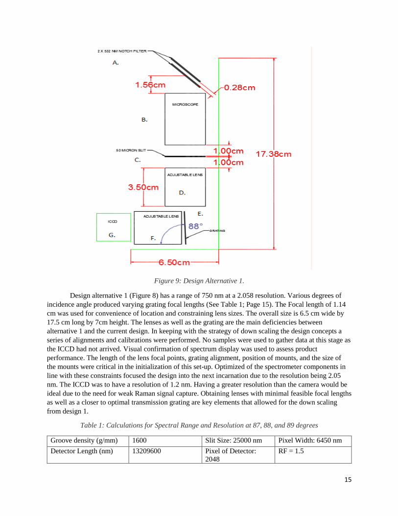
Figure 9: Design Alternative 1.

Design alternative 1 (Figure 8) has a range of 750 nm at a 2.058 resolution. Various degrees of

incidence angle produced varying grating focal lengths (See Table 1; Page 15). The Focal length of 1.14

cm was used for convenience of location and constraining lens sizes. The overall size is 6.5 cm wide by

17.5 cm long by 7cm height. The lenses as well as the grating are the main deficiencies between

alternative 1 and the current design. In keeping with the strategy of down scaling the design concepts a

series of alignments and calibrations were performed. No samples were used to gather data at this stage as

the ICCD had not arrived. Visual confirmation of spectrum display was used to assess product

performance. The length of the lens focal points, grating alignment, position of mounts, and the size of

the mounts were critical in the initialization of this set-up. Optimized of the spectrometer components in

line with these constraints focused the design into the next incarnation due to the resolution being 2.05

nm. The ICCD was to have a resolution of 1.2 nm. Having a greater resolution than the camera would be

ideal due to the need for weak Raman signal capture. Obtaining lenses with minimal feasible focal lengths

as well as a closer to optimal transmission grating are key elements that allowed for the down scaling

from design 1.

Table 1: Calculations for Spectral Range and Resolution at 87, 88, and 89 degrees

Groove density (g/mm) 1600 Slit Size: 25000 nm Pixel Width: 6450 nm

Detector Length (nm) 13209600 Pixel of Detector:

2048

RF = 1.5

16

Angle of Incidence Focal Length (nm) Sectral Range Calc

(nm/mm)

Resolution (nm)

87 20000000 235.192938 0.667676173

88 20000000 412.5412915 1.171140567

89 20000000 210.6010842 0.597863725

4.4.2 Alternate Design 2

This is a midway design arrangement incarnation. The components are as follows:

532nm notch filter (2 each): Semrock: 45° incident angle. The notch filter transmits 80% of

350 to 400 nm, 93% of 400 m to 513.2 nm, and 93% of 550.8 nm to1600 nm.

20 X Microscope: Edmond’s Scientific 20 x objective lens: 41.7 mm length x 15.3 mm width.

25 micron slit.

Focusing lens: 5 mm Thor Labs anti-reflective coated lens: 1 cm focal length

Dual Holographic transmission grating: 1600 groove/mm 45° transmission angle.

Collecting lens: 5 mm Thor Labs anti-reflective coated lens: 1 cm focal length

Figure 10: Design Alternative 2.

17

Figure 11: Visual Results of the Alternative Design

Design alternative 2 has a range of 300 nm at a 1.13 resolution. The overall size is 3.7 cm wide by

8.2 cm long by 7 cm height. The lenses were switched from the original design to achieve a shorter

overall focal length, from 3 cm focal lengths to 1 cm focal length. The deficiency in the capture lens was

discovered after alignment and thus the current design with a 2.54 cm diameter lens. Also the grating was

deficient as compared with current grating at 1200 L/mm vs 1600 L/mm. The arrangement of the ICCD

being perpendicular to the wrong reflectance angle is also corrected in the current design. The reflective

angle was initially to be 2° giving room to place the ICCD close to perpendicular to the transmission. This

proved a large enough angle to skew resolution (See Figure 9). Calculations and iterations of arrangement

and alignment the need for the ICCD to move exactly perpendicular to the transmission angle was

determined to be the optimal point of capture (See Table 2). Again this was visually confirmed after

calculations and arrangements were implemented due to the absence of an actual ICCD (see Figure 10).

Table 2: Calculations for spectral range and resolution based on focal length; blaze angle holding

resolution constant at 1 pixel per 1.136 nm. Highlighted data are the current measurements

Groove density (g/mm) 1600 Slit Size: 25000 nm Pixel Width: 6450 nm

Detector Length (nm) 13209600 Pixel # in Detector:

2048

RF = 1.5

Angle of Incidence Focal Length (nm) Spectral Range Calc

(nm/mm)

Resolution (nm)

45 10000000 433.705834 2.462446823

45 15000000 289.1372226 1.641631215

45 20000000 216.852917 1.231223411

45 25000000 173.4823336 0.984978729

45 30000000 144.5686113 0.820815608

18

5 REALISTIC CONSTRAINTS

Size and weight are constraints set forth by practicality and ergonomics of use for the instrument.

Transportation costs for space travel are exorbitant and the amount of material by launch creates the need

for instrumentation to be as efficient size and space wise as possible. The constraints set forth for size and

weight by NASA for this instrument are as follows:

i) The instrument aggregate size cannot exceed 25.40 cm x 25.30 cm x 20.32 cm

ii) Instrument weight cannot exceed 5kg.

These limitations are significant due to the impact on power capabilities of the laser. A more

powerful laser will return a stronger signal. In the Martian atmosphere the pressure is 5-7 Torr. This

fluctuation is significant due to the operating regions of the various types of laser spectroscopy being used

for this instrument. Attenuation of the signal is affected by atmospheric pressure. The pressure

fluctuations have the potential to overcome the benefits of this type of system if calculated compensation

is not instigated. The weight factor limits the types of materials that are allowed for casing and the

instrument internals. The environmental quality on Mars will be the primary constraining factor in

calibration and use of the integrated laser spectroscopy instrument.

The purpose of the spectrometer in this project is to get the most accurate reading while making

the smallest possible system. In pursuit of this goal, many complications arose. One of the more

significant problems was creating a large spectral image on the ICCD camera. This is important because

the more pixels the image occupies, the more detailed the reading will be. If the ICCD were to be placed

at the focal length of the capture lens, the image would be very detailed but very small in size. Despite the

clarity of the image, the resolution of the data reading would be bad because the spectral image does not

cover many pixels. To solve this problem, the ICCD was placed lightly before the focal length. While this

would reduce the clarity of the image, it would greatly increase the amount of pixels used in the data

collection. The calculation of this position is shown in Figure 8 page 16.

Figure 12: ICCD Position Calculation

As shown in Figure 8 page 16, the total focal length of the lens is 3 cm. The project light is

assumed to have a 2.5 mm buffer from each edge of the lens and the projected spectrum will be 1 cm in

19

width. This will cover a much larger area of pixels and also reduce the distance between the ICCD and

capture lens from 3 cm to 1.8 cm.

Another problem that occurred was the focal length errors of the focusing lens. The focusing lens

that was ordered from Thor Labs was designed to have a focal length of 1 cm but after testing, it was

discovered that the focal length was actually closer to 8 cm. The first components that was tested was the

focusing lens. It was removed from the spectrometer set-up and tested independently from the entire

system. This test showed that the focal length of the lens was truly 1 cm, which means that this was not

the cause of the problem. To isolate the source of the problem, the focusing lens was placed back on the

A-line and the slit, microscope objective and focusing lens were adjusted. The purpose of this test was to

see if the difference is distances between the slit, microscope objective and focusing lens would change

the focal length.

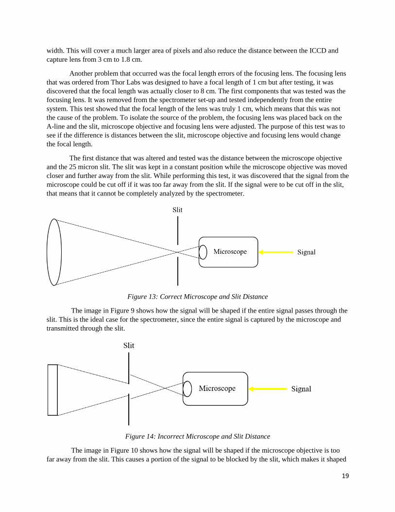
The first distance that was altered and tested was the distance between the microscope objective

and the 25 micron slit. The slit was kept in a constant position while the microscope objective was moved

closer and further away from the slit. While performing this test, it was discovered that the signal from the

microscope could be cut off if it was too far away from the slit. If the signal were to be cut off in the slit,

that means that it cannot be completely analyzed by the spectrometer.

Figure 13: Correct Microscope and Slit Distance

The image in Figure 9 shows how the signal will be shaped if the entire signal passes through the

slit. This is the ideal case for the spectrometer, since the entire signal is captured by the microscope and

transmitted through the slit.

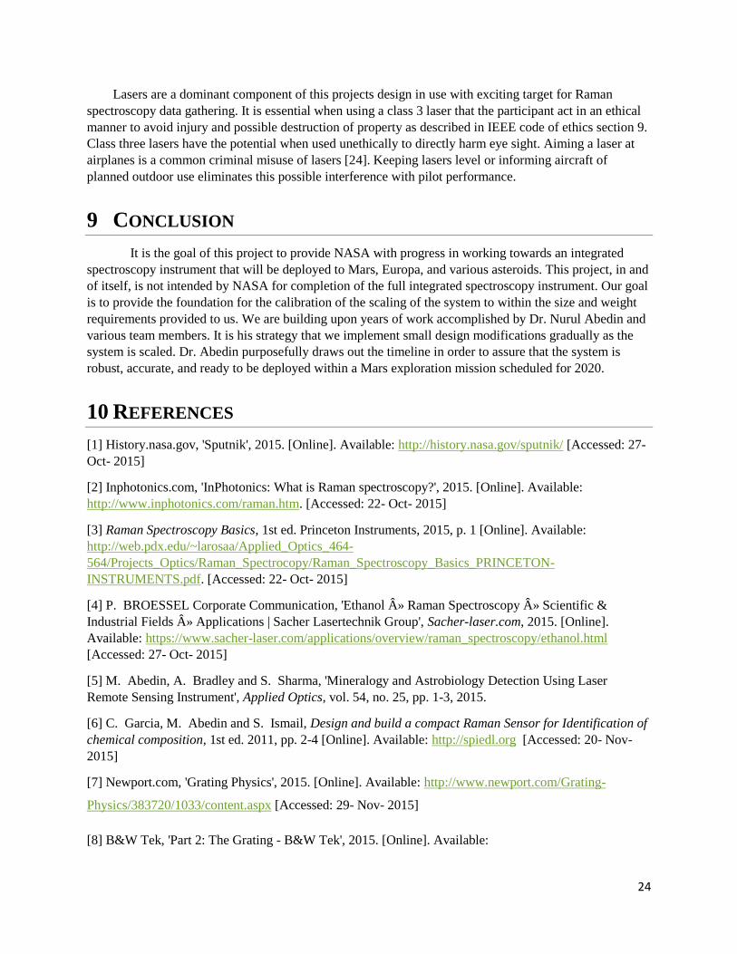
Figure 14: Incorrect Microscope and Slit Distance

The image in Figure 10 shows how the signal will be shaped if the microscope objective is too

far away from the slit. This causes a portion of the signal to be blocked by the slit, which makes it shaped

20

as such. If this occurs, then the entire signal will not be captured and analyzed by the spectrometer.

Although this was an important discovery on how to get a better signal, this distance did not affect the

focal length of the focusing lens. With this in mind, the slit and microscope object was placed at the

optimal position and then the focusing lens position was altered. Like the distance with the microscope

objective and slit, there was a certain distance that, if placed, the lens would not capture the entire signal.

Figure 15: Theoretical Lens Projection

As shown in Figure 11, the light that passes through the lens should focus to the sharpest point at

1 centimeter away from the lens. This assumption comes from the independent testing of the focusing

lens. However, once the lens was placed at an appropriate distance, the focal length of the light turned out

to be much larger.

Figure 16: Actual Lens Projection

Figure 12 shows the how the light actually comes out of the lens. The light no longer goes to a

point but rather a smaller circle. Once it passes this small circle, it starts to get larger again and more

distorted. The light also did not reach this ideal circle in 1 centimeter. The circle point was not reached

until about 8 centimeters away from the lens. No matter what distance the focusing lens was placed away

from the slit, this focal length did not change. With this fact in mind, it was concluded that this increase in

focal length was due to the spreading of light from the microscope objective. Like the lens, the

microscope objective focuses the lens at a certain point but after this point is passed, the light begins to

get larger again. After the focused light passes through the slit, it begins to get larger even as it goes into

the focusing lens. As the light passes through the focusing lens, it attempts to focusing the light into a

point while the light is still increasing in size. These two properties fight against each other until it

reaches the sharpest circle at 8 centimeters. Normally, this problem could be solved by moving the lens

closer to the slit but the mounts for both of the components prevent them from getting too close to each

other.

21

6 IMPACTS OF THE DESIGN

6.1 ECONOMIC This is not the first rover that has been sent into space, so the cost of sending a rover is already

well established. According to NASA, the cost of the Mars Pathfinder Rover mission was approximately

$265 million- [11]. This cost comes from building, testing, operating, and eventually launching the rover

to Mars. The equipment on the Pathfinder was designed to operate in different atmospheric conditions

while simultaneously being the most compact it possible can [12]. The proposed design follows in these

footsteps because it will have an impact on the building cost of the rover. This cost comes from not only

from purchasing and constructing the device but also how large and heavy the final system is. The heavier

the system is; the more fuel it will cost to send into space. In order to alleviate some of this cost, the

device is given a weight and size restriction.

6.2 ENVIRONMENTAL Whenever an object is introduced to a new environment, it takes part in a bacteria and germ

exchange. All people and objects have some sort of new bacteria on them and they pass it on to anything

or anyone they interact with. The same rule applies to our system. It is covered in bacteria from the

engineers working on it and even from the air. When this system is eventually sent to Mars, these bacteria

will be exposed to entirely new environment. This is a significant issue because this will effective

introduce a new set of bacteria and contaminants to an unprotected environment. Contamination of the

Mars environment presents two keys issues in the system’s operations. The first is that the system could

identify these substances and mistakenly identify that they originated from Mars. The second is that an

unintentional reaction could happen between the natural contaminates on Mars and the ones that are

brought there, which will also cause invalid data. To solve this issue, the engineers can completely isolate

the system inside its housing. That means that even if there is contaminates on the system’s components,

they will be introduced to the new environment. By doing this, the system and Mars’s environment are

protected from each other.

6.3 HEALTH & SAFETY The multispectral instrument that is being constructed uses a high-powered laser to initiate the

spectroscopies. All lasers, even common laser pointers, are very dangerous if looked at directly and at

higher power, laser can even damage the surface of the skin. According to the Laser Safety Manual

provided by Old Dominion University – [13], the user of a laser should always have the proper training

before operating any system with a laser in it. This rule applies to the compact multispectral instrument as

well. Before anyone uses it, they should receive a proper course and laser safety so that injuries to others

and themselves can be better avoided.

6.4 CONTEMPORARY ISSUES The primary function of this system is to analyze substances on Mars using four different types of

spectroscopies. Each of these spectroscopies have a wide array of uses, from LIDAR being used for

geographical profiling- [14] to LIF being used in plasma research- [15]. With all of these strengths and

uses put together, our system has the potential to be applied in other fields or research. One that comes to

mind is the identification of biological substances. Raman and LIF spectroscopies are commonly used in

cancer cure studies to identify the composition of a cell or tumor. This process is already being applied by

22

scientist in identifying and characterizing colon cancer – [16]. With this knowledge, biologists are able to

develop a countermeasure with the hope of eliminating the disease. Since our system will employ both of

these spectroscopies and will also be small in size, it is possible that this system could eventually be

adapted for biological studies.

7 LIFELONG LEARNING

7.1 KNOWLEDGE FROM OTHER COURSES Old Dominion University offers a vast amount of engineering classes. Among these classes, there

were three in particular that were instrumental in the team’s performance on this project. The first one is

ECE 478: Introduction to Lasers and Laser Applications. This class taught the fundamentals of how lasers

operate and what functions they could perform. This class provided the team with a baseline of

knowledge that could be used to tackle this project. The second important class is ECE 303: Introduction

to Electric Power. This class describes how electrical current and power can be used in everyday

applications and it also gave students exposure to high voltage cases. This is very important because it not

only taught the team high voltage safety, but it also gave valuable information on how to work with these

high voltages effectively. The last class that provided the team with key knowledge was ECE 381:

Introduction to Discrete-time Signal Processing. This class taught the fundamentals behind analyzing

discrete electronic signals and it also provided Mat Lab instruction. Mat Lab programing was

implemented in this system and ECE 381 provided a much needed foundation to this programing

language.

7.1.1 James Hornef

After working on this project, I realized that some concepts cannot be mastered from a book.

When Jay and I were first exposed to the four types of spectroscopy, they seemed to be too hard to grasp

on paper. However, once we were able to perform tests involving these spectroscopies, we realized they

were very manageable. This project taught us a valuable lesson in being active in one’s learning and

understanding of concepts. This project also taught me to more independent in moving forward in a

project. During school, I have become accustom to being told what to do to accomplish a task but with

this project, it was entirely up to Jay and I to formulate a plan and go through with it.

This project has also taught me that it is very important to have a complete understanding of the

design before ordering components for it. This realization came after Jay and I began to build our first

design. We were not aware of some constraints of the spectrometer, such as the position of the capture

lens and the collection of signal from this lens. Without taking these facts into account, the capture lens

was designed to be the same size as the capture lens, which is rather small, and led to the discovery that

the capture lens did not collect all of the spectrum created by the white light source. This oversight caused

a delay in the project until a larger lens could be ordered. After making this mistake, it made me realized

how important it is to thoroughly go through a design before ordering parts.

7.1.2 John F. Lucas (Jay)

General physics is taught to every student entering into science and technology fields of study.

When research and design projects are undertaken the theory that is learned becomes execution of the

experiment and outcome in the results. This project has brought recollection of the base concepts that

were presented to me when I began my engineering degree at ODU. It has coupled this theory with more

advanced concepts in lasers and analysis procedures. The theory utilized in this project has been coupled

23

with inherit mission challenges and interpersonal communications and understanding of principals

through different opinions. The ability to work within a group, albeit small in this case, is emphasized

through the project’s execution. When each team member contributes in a positive manner the project

grows beyond the initial concepts to a learning platform that can be applied to other areas of study and

work life. The more opinions expressed about sound theory can lead to enlightenment or can befuddle the

participants through miscommunication or misunderstood concepts. The proposal process has brought a

variety of these challenges and presented directions and schemes for learning to continue through

discipline and concepts absorbed.

8 ENGINEERING STANDARDS

ASNI Z136.1-2007 [17]: The American Nation Standard for Safe Use of Lasers. This standard

describes the safe practices for laser use. This project will test the Laser spectrometer instrument that is

being designed and implemented. In order to securely handle the laser used to produce the LIF, LIBS,

Raman, and LIDAR feedback safety standards are being implemented.

ASTM STP1066 Laser Techniques in Luminescence Spectroscopy [18]: The American Society

for Testing and Materials STP1066 is being used as a guide for calibration and to implement standards for

spectroscopy techniques. In order to understand and implement design optimisation for an effective

design layout the process of spectroscopy needs to be understood from a standardized perspective.

NASA-STD-(I)-0007 NASA Computer-Aided Design Interoperability [19]: The layouts for the

design proposal will be made into a functioning prototype. In order to convey spectrometer element

location information accurately AutCAD has been used. In order to convey the information within NASA

it is necessary to conform to their styles and standards for a computer-aided design.

NASA-STD 8739.6: Implementation Requirements for NASA Workmanship Standards [19]:

This project requires a prototype assembly to be built and augmented as bench testing and calibration is

administered. In order to meet qualifying requirements for workmanship the standards for NASA

workmanship requirements must be applied.

ANSI Z136.1 Laser Safety [20]: This project used a variety of class 3 lasers. In order to ensure

proper and safe use of the lasers bot James and Jay were required by NASA to pass a laser safety course

that is governed by the ANSI Z136.1 Laser safety standard.

ASTM E2078-00(2010) Standard Guide for Analytical Data Interchange Protocol for Mass

Spectrometric Data [21]: Data collection protocols allow for elimination of distortion in data gathering.

The elimination of the distortion from various sources allows for trouble shooting techniques that can

eliminate various sources of unintended information alteration.

ASTM E1578-13 Standard Guide for Laboratory Informatics [22]: The information that is

gathered during the experiments needs to be presented in a standardized and formal format. This standard

enables the formatting of information into a professional data log for later presentation.

IEEE Code of Ethics [23]: The disclosure of intricate and secret information by an engineer on

the project or the company they are working for is unethical and illegal. The subject matter of this project

can be disclosed with omission of some specifics to avoid a conflict of interest with NASA and ODU.

However, the possibility exists for conflict of interest to exist and section 2 of the IEEE code of ethics

informs engineers of what may fall into ethical or unethical conduct.

24

Lasers are a dominant component of this projects design in use with exciting target for Raman

spectroscopy data gathering. It is essential when using a class 3 laser that the participant act in an ethical

manner to avoid injury and possible destruction of property as described in IEEE code of ethics section 9.

Class three lasers have the potential when used unethically to directly harm eye sight. Aiming a laser at

airplanes is a common criminal misuse of lasers [24]. Keeping lasers level or informing aircraft of

planned outdoor use eliminates this possible interference with pilot performance.

9 CONCLUSION

It is the goal of this project to provide NASA with progress in working towards an integrated

spectroscopy instrument that will be deployed to Mars, Europa, and various asteroids. This project, in and

of itself, is not intended by NASA for completion of the full integrated spectroscopy instrument. Our goal

is to provide the foundation for the calibration of the scaling of the system to within the size and weight

requirements provided to us. We are building upon years of work accomplished by Dr. Nurul Abedin and

various team members. It is his strategy that we implement small design modifications gradually as the

system is scaled. Dr. Abedin purposefully draws out the timeline in order to assure that the system is

robust, accurate, and ready to be deployed within a Mars exploration mission scheduled for 2020.

10 REFERENCES

[1] History.nasa.gov, 'Sputnik', 2015. [Online]. Available: http://history.nasa.gov/sputnik/ [Accessed: 27-

Oct- 2015]

[2] Inphotonics.com, 'InPhotonics: What is Raman spectroscopy?', 2015. [Online]. Available:

http://www.inphotonics.com/raman.htm. [Accessed: 22- Oct- 2015]

[3] Raman Spectroscopy Basics, 1st ed. Princeton Instruments, 2015, p. 1 [Online]. Available:

http://web.pdx.edu/~larosaa/Applied_Optics_464-

564/Projects_Optics/Raman_Spectrocopy/Raman_Spectroscopy_Basics_PRINCETON-

INSTRUMENTS.pdf. [Accessed: 22- Oct- 2015]

[4] P. BROESSEL Corporate Communication, 'Ethanol » Raman Spectroscopy » Scientific &

Industrial Fields » Applications | Sacher Lasertechnik Group', Sacher-laser.com, 2015. [Online].

Available: https://www.sacher-laser.com/applications/overview/raman_spectroscopy/ethanol.html

[Accessed: 27- Oct- 2015]

[5] M. Abedin, A. Bradley and S. Sharma, 'Mineralogy and Astrobiology Detection Using Laser

Remote Sensing Instrument', Applied Optics, vol. 54, no. 25, pp. 1-3, 2015.

[6] C. Garcia, M. Abedin and S. Ismail, Design and build a compact Raman Sensor for Identification of

chemical composition, 1st ed. 2011, pp. 2-4 [Online]. Available: http://spiedl.org [Accessed: 20- Nov-

2015]

[7] Newport.com, 'Grating Physics', 2015. [Online]. Available: http://www.newport.com/Grating-

Physics/383720/1033/content.aspx [Accessed: 29- Nov- 2015]

[8] B&W Tek, 'Part 2: The Grating - B&W Tek', 2015. [Online]. Available:

25

http://bwtek.com/spectrometer-part-2-the-grating/ [Accessed: 29- Nov- 2015]

[9] Semrock.com, 'Semrock - Part Number: NF03-532E', 2015. [Online]. Available:

https://www.semrock.com/FilterDetails.aspx?id=NF03-532E-25 [Accessed: 29- Nov- 2015].

[10] Syntronics.net, 'Syntronics, LLC - Min-I-Cam', 2015. [Online]. Available:

http://www.syntronics.net/min-i-cam.html [Accessed: 27- Nov- 2015].

[11] Nssdc.gsfc.nasa.gov, 'NASA - NSSDC - Spacecraft - Details', 2015. [Online]. Available:

http://nssdc.gsfc.nasa.gov/nmc/spacecraftDisplay.do?id=MESURPR [Accessed: 27- Oct- 2015]

[12] NASA Facts, 1st ed. Pasadena: NASA, 2015, pp. 1-3 [Online]. Available:

http://www.jpl.nasa.gov/news/fact_sheets/mpf.pdf [Accessed: 27- Oct- 2015]

[13] Old Dominion University Laser Safety Manual, 1st ed. Norfolk: Environmental Health and Safety

Office, 2015, pp. 23-24 [Online]. Available:

https://www.odu.edu/content/dam/odu/offices/environmental-health-safety/docs/laser-safety-manual.pdf

[Accessed: 28- Oct- 2015]

[14] Lidar-uk.com, 2015. [Online]. Available: http://www.lidar-uk.com/usage-of-lidar/ [Accessed: 28-

Oct- 2015]

[15] E. Scime, C. Biloiu, C. Compton, F. Doss, D. Venture, J. Heard, E. Choueiri and R. Spektor,

'Laser induced fluorescence in a pulsed argon plasma', Rev. Sci. Instrum., vol. 76, no. 2, p. 026107, 2005.

[16] S. Li, G. Chen, Y. Zhang, Z. Guo, Z. Liu, J. Xu, X. Li and L. Lin, 'Identification and

characterization of colorectal cancer using Raman spectroscopy and feature selection techniques', Opt.

Express, vol. 22, no. 21, p. 25895, 2014.

[17] ASNI Z136.1-2007, 1st ed. Orlando, Fla.: Laser Institute of America, 2015, pp. 1-81. [PDF]

Available: https://www.lia.org/PDF/Z136_1_s.pdf [Accessed: 23- Nov- 2015]

[18] T. Vo-Dinh and D. Eastwood, ASTM STP1066 Laser Techniques in Luminescence Spectroscopy, 1st

ed. Chelsea, MI: AMERICAN SOCIETY FOR TESTING AND MATERIALS, 1990.

[19] Standards.nasa.gov, '.. NASA Technical Standards Program ..', 2015. [Online]. Available:

https://standards.nasa.gov/documents/detail/3315683 [Accessed: 30- Nov- 2015].

[20] S. Oleson, "ANSI Z136.1 - Safe Use of Lasers - LIA", Lia.org, 2016. [Online]. Available:

https://www.lia.org/publications/ansi/Z136-1 [Accessed: 17- Mar- 2016].

[21] D. Inc., "ASTM-E2078 | Standard Guide for Analytical Data Interchange Protocol for Mass

Spectrometric Data | Document Center, Inc.", Document-center.com, 2016. [Online]. Available:

https://www.document-center.com/standards/show/ASTM-E2078 [Accessed: 17- Mar- 2016].

[22] "ASTM E1578-13 - LIMSWiki", Limswiki.org, 2016. [Online]. Available:

http://www.limswiki.org/index.php?title=ASTM_E1578-13 [Accessed: 17- Mar- 2016].

26

[23] Ieee.org, 'IEEE IEEE Code of Ethics', 2015. [Online]. Available:

http://www.ieee.org/about/corporate/governance/p7-8.html [Accessed: 27- Nov- 2015].

[24] "Laser Pointer Safety - NEVER aim laser pointers at aircraft", Laserpointersafety.com, 2016.

[Online]. Available: http://www.laserpointersafety.com/laser-hazards_aircraft/laser-hazards_aircraft.html.

[Accessed: 17- Mar- 2016].

11 APPENDIX A: MEETING LOG

Week one (9/11/2015):

This was the first week at the NASA Langley Labs. The day was spent getting acquainted with

the laboratory and its equipment. Dr. Abedin showed us around the building and told us where we could

get any supplies that we need. Dr. Abedin also introduced us to the system we would be working on. He

took us step by step on how to use the system to read a neon light source. We then played around with

this acquired data by eliminating the background noise and using a given reference to convert the signal

into a wavelength chart.

Week Two (9/18/2015):

This week Dr. Abedin taught us how to turn a wavelength chart into a Raman scattering chart,

using the same software as before. He also taught us the math behind this conversion so it could be

checked for correctness. After the lesson, he left us to convert a signal measurement of sulfur from the

pixel format to the Raman format. After many trail error attempts, the Raman that we produced at the end

was within 50 cm^ (-1) of the correct readings. To get the correct readings, we ended up using the

formulas he provided to calculate each point manually. This ended up giving us the correct result.

Week Three (9/25/2015):

This week Dr. Abedin gave us an overview of how the system worked. He explained each step in

greater detail than he did on the first week. This was vital because our project uses this exact set-up. He

also gave us documents to read so we would become more familiar with the terminology used through

this project. After we read the papers, Dr. Abedin gave us the design specifications of our project. This

allowed us to start thinking how to build this device so it would be within these limits.

Week Four (Thursday 10/1/2015)

Today we meet with Dr. Ali and discussed more optimal ways to learn the material. We all agreed

that instead of trying to learn all four types of spectroscopy at once that we would focus on one at a time.

In accordance of this new decision, we were assigned to create a 4-6 slide PowerPoint presentation on

Laser Induced Breakdown Spectroscopy. This presentation will be due next Thursday and Thursday

meetings with Dr. Ali will now become a regular thing.

*We did not go into the lab on Friday 10/2/2015 due to a hurricane warning.

Week Five

Thursday 10/8/2015:

Since the last meeting, James created the PowerPoint for LIBS and also wrote the preliminary

proposal due for the 486 class. James sent these files to Jay, who proofed read them and added images to

27

the report. Today we presented Dr. Ali our slides on LIBS and discussed the topic further. We learned

about a database that has the atomic characteristics of virtually every type of atom. We also were

informed about a reference website called Science Direct, which publishes scientific journals on a wide

variety of topics. Dr. Ali gave us our second assignment, which was to find 4-5 research papers on LIBS.

The key topic he wants us to focus on is papers involving space conditions.

Friday 10/9/2015:

James arrived to the lab at 10:30am and discussed aspects of the project with Dr. Abedin. Jay

arrived at the lab shortly after at 11 am and we were both tasked with reading the manuals on the ICCD

camera and Nd: YAG 1064 nm laser. We read these manuals till about 1:30 pm and then James went into

the lab and found more documents of interest to the project. Jay and James proceeded to read some of

these documents until 2:30 pm when Jay left. James stayed behind to perform more research and to

organize this new material. James also organized the lab in such a way that he and Jay could easily find

all the materials that relate to their project. James completed this task by 3:30 pm and then assisted Dr.

Abedin with calibrating a new spectrometer. James was able to learn how to operate this new

spectrometer and learn more about how to record data with it. James left the lab at 4:30 pm.

Week Six:

Thursday 10/15/2012:

Before coming to this meeting, Jay and James read two research papers each involving LIBS.

These papers were then highlighted for key details and presented to Dr. Ali. While Dr. Ali skimmed the

papers that were provided, Jay and James described the core foundation of each paper. Jay’s papers talked

about the history of LIBs and the use of LIBs on a specific element found on Mars. James’s papers talked

about using LIBs in space simulated atmospheres and how these different conditions effected the

measurements of the systems. Once all of the papers were reviewed, Jay and James decided that they

would focus on writing the midterm proposal this week rather than moving on to the next spectroscopy.

Dr. Ali agreed that this was a wise choice and said he would look over the draft created by the next

meeting.

Friday 10/16/2015:

Due to an unforeseen error at the Bioelectrics lab, James was unable to attend the scheduled

meeting at NASA Langley. Jay however was able to make it and would fill James in on what he missed.

Week Seven:

Thursday 10/22/2015:

Dr. Ali permitted each group to have a week extension to turn in the proposal. With this in mind,

Jay and James used this time to fine tune the report so it could be even better. Dr. Ali also agreed that the

direction of the project needed to be changed since there wasn’t much design work going on. Dr. Ali,

James and Jay decided that the project should steer in the direction of building a spectrometer. Once the

paper was completed, research would begin on the spectrometer.

Friday 10/23/2015:

Today, Jay and James discussed the project idea with Dr. Abedin and he agreed that building a

spectrometer would be a good design idea. Dr. Abedin suggested that the two of them research the parts

that make up a spectrometer. Research was continued until Dr. Abedin left the lab.

28

Week Eight:

Thursday 10/29/2015:

There was no meeting with Dr. Ali today due to the fact he was absent from class. Jay and James

submitted the hard copy of the Midterm proposal to his box.

Friday 10/29/2015:

Jay was kept up at work today and was unable to make it to NASA. James arrived at the lab and

continued his research on spectrometers and found equations that could be used to design and calibrate

the spectrometer.

Week Nine:

Thursday 11/5/2015

Today, Jay and James talked to Dr. Ali about the progress being made on the spectrometer. Dr.

Ali suggested that a few parameters be focused on while designing the spectrometer. Dr. Ali suggested on

focusing on the resolution, spectral range and precision of the spectrometer. Dr. Ali also suggested that

the exact part numbers of the components used in the spectrometer be detailed in the project.

Friday 11/6/2015

Dr. Abedin requested that a design be created in AutoCAD so it could be made by the machine

shop at NASA. This design would be the cornerstone of our final design proposal. This design was

created using the equations found during the research of the spectrometer. With this in mind, this meeting

was focused on the general orientation of the design. Also, Jay and James needed to create a presentation

to detail what was being done in the project. This presentation was dated for next Thursday and Jay

insisted on creating the PowerPoint. This PowerPoint was passed back and forth between Jay and James

in for corrections and improvements throughout the week.

Week Ten:

Thursday 11/12/2015

Today was the presentation of the current progress of the project. The presentation showed the

equations used to design the layout and the first draft of the AutoCAD design. After the presentation was

completed, a progress update was given to Dr. Ali. Dr. Ali suggested that there should be more focus on

the ICCD camera and the type of notch filter being used in the spectrometer.

Friday 11/13/2015

Jay and James were running into dead ends with the calculations used to create the AutoCAD

design. Dr. Abedin was able to provide a practical example of the equation usage and walked Jay and

James through the procedure. Thanks to Dr. Abedin’s help, Jay and James were able to complete the

calculations for the spectrometer they were designing. Using this equation, James was able to create an

excel chart for all of the possible conditions that could be used in the spectrometer. With this data sheet,

Jay and James could now pick the most optimal design possible for the given parts.

Week Eleven:

Thursday 11/19/2015

29

Jay and James gave an update about their progress on the project. James showed Dr. Ali the

calculations from the excel sheet and Jay showed Dr. Ali his AutoCAD progress. Jay asked why there

isn’t’ bench testing being performed before the design is made. Bench testing would provide Jay and

James with very relevant data that could help optimize the design of the spectrometer. Dr. Ali agreed that

bench testing would be beneficial to the design process.

Friday 11/20/2015

Jay and James continued work on the AutoCAD design. Jay and James did not want to submit a

design that could have potential errors in it. Jay also brought up the bench testing issue to Dr. Abedin and

Dr. Abedin agreed that it would be a good idea. Also, since the final proposal was due in 2 weeks, Jay and

James divided up the work required to complete the report and plan on giving Dr. Ali and Dr. Abedin a

rough draft by Thursday.

Week Twelve:

Note: We did not meet this week since it was Thanksgiving weekend.

*Other than these meetings at NASA and with Dr. Ali, James and Jay kept in constant contact with each

other through various email chains. Due to schedule complications, this proved to be the most effective

method to communicate.

Second Semester:

Week 1 (1/3-1/9): Over the break, the group designed and constructed multiple spectrometer designs.

These designs gave the group better insight in how to optimize the final product. With this in mind, the

group began to order parts for the final design. This final design was drafted on AutoCAD and was

designed to be much smaller than all the previous designs.

Week 2 (1/10- 1/16): The group finalized the part order for the newest design and submitted it to Dr.

Abedin. The order was sent early in the week so the parts arrived toward the end, allowing the group to

assemble the system.

Week 3 (1/17 – 1/23): The system was assembled last week but this week, the design was disassembled

and placed on a mobile platform. Once it was placed on the mobile platform, it was aligned using the

white light source. The image produced was very sharp but it did not display the deepest reds or deepest

violets.

Week 4 (1/24 – 1/30): Given last week’s discovery, the system was optimized to display the most range

of light possible. Once this was completed, the 639 laser was used in place of the white light source to see

if the alignment was correct. This was implemented outside of the spectrometer system with the dichroic

mirror and targeting mirrors. Once this laser alignment was completed, the same procedure was repeated

with a neon light source and a 532 laser light source.

Week 5 (1/31 – 2/6): A new member was added to the group this week, so this week was spent aiding the

newest member and catching them up on what was being done. This was done by sharing resources and

playing with the currently constructed system.

30

Week 6 (2/7- 2/13): There was a midterm presentation due this week so the 487 portion of the group spent

this week preparing and practicing for this presentation.

Week 7 (2/14 – 2/20): The group spent this week optimizing the current system design. This was done by

leveling every component, ensuring everything is exactly the same height and aligning everything to

exactly the correct angles. This required the group to disassemble the system and reassemble it. The result

were the most optimal projections and ranges. The ICCD camera also arrived this week, so the group also

read up on the manual in order to operate the camera without damaging it.

Week 8 (2/21 – 2/27): Since the current system was completely optimized, the final alterations were

finally made. The group decided to order a new type of alignment system that connected each of the parts

to each other, aligning the to exactly the correct height, angle and position. This would potentially reduce

alignment time significantly. The group also decided to order a new microscope lens, since it was the only

part in the system that was not specifically ordered for the project. Finally, the group installed the ICCD

camera software onto to laptop to be used in the data collection, but it was soon realized that there were

some connection issues between the camera and the PC. To fix this problem, new parts and to be ordered

for the computer, which would resolve the connection issues and allow the camera to record data.

Week 9 (2/28- 3/5): Since the newest parts have yet to arrive, the group spent this week reading the new

ICCD camera manual and designing a mount to hold the camera. The design was drafted and

manufactured this week and will be implemented in the final design.

Week 10 (3/6 – 3/12): The group did not meet this week due to spring break and the fact that the newest

parts have yet to arrive. The construction of the new system will be finished next week, when all of the

parts arrive. The group also designed a mounting plate for the ICCD camera and left the design in the

metal shop for assembly.

Week 11 (3/13-3/19): The newest components arrived in the lab today and the team spent the week

assembling, testing and aligning the system. Some components needed to be altered in order to work with

the newest parts so the team drafted some alterations to the components and sent them to the meatl shop

for reconstruction.

Week 12 (3/20-3/36): With the newest version of the system complete, the group moved on to installing

and configuring the programs used to control the ICCD camera. There were minor problems with the

laptop permissions so it had to be sent to the IT department to be worked on.

Week 13 (3/27-4/2): With the laptop fully operational, the team was able to finish wiring the camera to

computer. The ICCD was able to pick up a fluorescence signal from the light white source and a portion

of the neon light source.

Week 14 (4/3-4/9): The 487 portion of the group met this week to work on the poster and to divide up the

work for the final presentation and paper. It was discovered that the system was still not aligned properly

so the team fixed the issue.

Week 15 (4/10-4/16): The group continued to work with the ICCD camera with various samples. Samples

for neon and ruby crystal were successfully acquired. Other samples such as marble, granite and

naphthalene were used but no strong signal was found.

Week 16 (4/17-4/23): The 487 team worked on completing the final report and began practicing for the

final presentation on the 26th.