ECO 120- Macroeconomics

Weekend School #121st April 2007

Lecturer: Rod DuncanPrevious version of notes: PK Basu

Topics for discussion

• Module 1- macroeconomic variables

• Module 2- basic macroeconomic models

• Module 3- savings and investment

• What will not be discussed– Answers to Assignment #1 (use the CSU

forum for this)

Forms of economics

• Microeconomics- the study of individual decision-making– “Should I go to college

or find a job?”– “Should I rob this

bank?”– “Why are there so

many brands of margarine?”

• Macroeconomics- the study of the behaviour of large-scale economic variables– “What determines

output in an economy?”

– “What happens when the interest rate rises?”

Economics as story-telling

• In a story, we have X happens, then Y happens, then Z happens.

• In an economic story or model, we have X happens which causes Y to happen which causes Z to happen.

• There is still a sequence and a flow of events, but the causation is stricter in the economic story-telling.

Kobe, the naughty dog

Modelling Kobe

• Kobe likes to unmake the bed.

• Kobe likes treats.

• We assume that more treats will lead to fewer unmade beds.

(Not a very good) Model:

Treats↑ → Unmaking the bed↓

• We can use this model to explain the past or to predict the future.

Elements of a good story

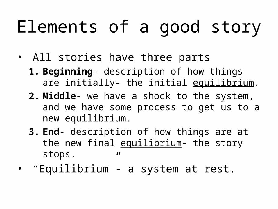
• All stories have three parts1. Beginning- description of how things are

initially- the initial equilibrium.

2. Middle- we have a shock to the system, and we have some process to get us to a new equilibrium.

3. End- description of how things are at the new final equilibrium- the story stops.

• “Equilibrium”- a system at rest.

Timeframes in economics

• In economics we also talk in terms of three timeframes:– “short run”- the period just after a shock has occurred

where a temporary equilibrium holds.– “medium run”- the period during which some process

is pushing the economy to a new long run equilibrium.– “long run”- the economy is now in a permanent

equilibrium and stays there until a new shock occurs.

• You have to have a solid understanding of the equilibrium and the dynamic process of a model.

What are the big questions?

• What drives people to study macroeconomics? They want solutions to problems such as:– Can we avoid fluctuations in the economy?– Why do we have inflation?– Can we lower the unemployment rate?– How can we manage interest rates?– Is the foreign trade deficit a problem?– [How can we make the economy grow faster?] Not

taken up in this class. This class focuses on short-run problems.

Economic output

• Gross domestic product- The total market value of all final goods and services produced in a period (usually the year).– “Market value”- so we use the prices in

markets to value things– “Final”- we only value goods in their final form

(so we don’t count sales of milk to cheese-makers)

– “Goods and services”- both count as output

Measuring GDP

• Are we 40 times (655/16) better off than our grandparents?

– Australian GDP in 1960- $15.6 billion– Australian GDP in 2000- $655.6 billion

• What are we forgetting to adjust for?

Measuring GDP

• Population- Australia’s population was 10 million in 1960 and 19 million in 2000.– GDP per person in 1960 = $15.6 bn / 10m

= $1,560– GDP per person in 2000 = $655.6 bn / 19m

= $34,500

• Prices- $1,000 in 1960 bought a better life-style than $1,000 in 2000.

Nominal versus real GDP

• So how to correct for rising prices over time?– Measure average prices over time (GDP

deflator, Consumer Price Index, Producer Price Index, etc)

– Deflate nominal GDP by the average level of prices to find real GDP

Real GDP = Nominal GDP / GDP Deflator

Nominal versus real GDP

• We use prices to value output in calculating GDP, but prices change all the time. And over time, the average level of prices generally has risen (inflation). – Nominal GDP: value of output at current

prices– Real GDP: value of output at some fixed set

of prices

Some Australian economic historyAustralian GDP 1950-1995

0

100 000

200 000

300 000

400 000

500 000

600 000

1950 1960 1970 1980 1990 2000

Mil

lio

n A

$

GDP

GDP Change

Real GDP

Business cycle

• The economy goes through fluctuations over time. This movement over time is called the “business cycle”. – Recession: The time over which the economy is

shrinking or growing slower than trend– Recovery: The time over which the economy is

growing more quickly than trend– Peak: A temporary maximum in economic activity– Trough: A temporary minimum in economic activity.

Australian business cycleAust Business Cycle

-4

-2

0

2

4

6

8

10

1950 1960 1970 1980 1990 2000

% Ch RGDP

Unemployment

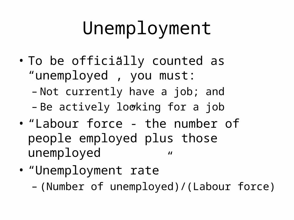
• To be officially counted as “unemployed”, you must:– Not currently have a job; and– Be actively looking for a job

• “Labour force”- the number of people employed plus those unemployed

• “Unemployment rate”– (Number of unemployed)/(Labour force)

Unemployment

• Working age population = Labour force + Not in labour force

• Labour force = Employed + Unemployed

UnemploymentUnemployment over the Business Cycle

-4

-2

0

2

4

6

8

10

12

1965 1968 1971 1974 1977 1980 1983 1986 1989 1992 1995

Pe

rce

nt

(%)

Unemployment

Change in GDP

Inflation

• Inflation is the rate of growth of the average price level over time.

• But how do we arrive at an “average price level”?– The Consumer Price Index surveys

consumers and derives an average level of prices based on the importance of goods for consumers, ie. a change in the price of housing matters a lot, but a change in the price of Tim Tams does not.

Consumer Price Index

• Then the CPI expresses average prices each year relative to a reference year, which is a CPI of 100.CPIt = (Average prices in year t)/(Average

prices in reference year) x 100

• Inflation can then be measured as the growth in CPI from the year before:– Inflationt = (CPIt – CPIt-1) / CPIt-1

InflationConsumer Price Inflation

-2.0

0.0

2.0

4.0

6.0

8.0

10.0

12.0

14.0

16.0

18.0

20.0

Sep

-70

Sep

-72

Sep

-74

Sep

-76

Sep

-78

Sep

-80

Sep

-82

Sep

-84

Sep

-86

Sep

-88

Sep

-90

Sep

-92

Sep

-94

Sep

-96

Sep

-98

Sep

-00

Sep

-02

Sep

-04

Inflation

Calculating GDP

• Gross domestic product- The total market value of all final goods and services produced in a period (usually the year).

• Alternates methods of calculating GDP– Income approach: add up the incomes of all members

of the economy– Value-added approach: add up the value added to

goods at each stage of production– Expenditure approach: add up the total spent by all

members of the economy• The expenditure approach forms the basis of the

AD-AS model.

Expenditure approach

• GDP is calculated as the sum of:– Consumption expenditure by households (C)– Investment expenditures by businesses (I)– Government purchases of goods and services

(G)– Net spending on exports (Exports – Imports)

(NX)

Aggregate Expenditure: AE = C + I + G + NX

Consumption and savings

• We assume consumption (C) depends on household’s disposable income: – Disposable income YD = (Income – Taxes)

• The consumption function shows how C changes as YD changes.

• Household savings (S) is the remainder of disposable income after consumption.

• The savings function shows how S changes as YD changes.

Properties of a consumption function

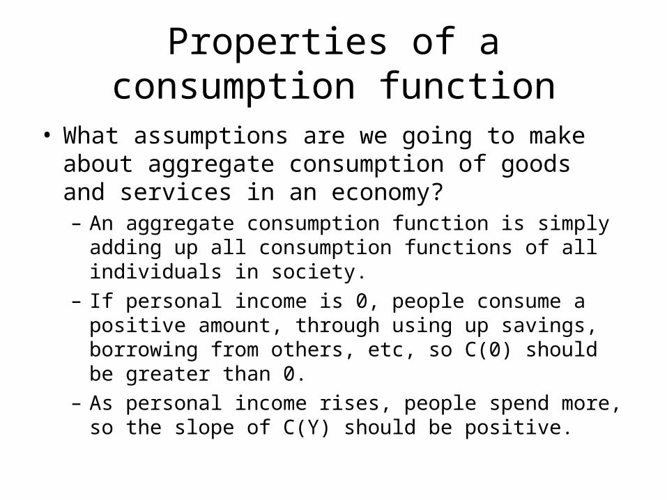
• What assumptions are we going to make about aggregate consumption of goods and services in an economy?– An aggregate consumption function is simply adding

up all consumption functions of all individuals in society.

– If personal income is 0, people consume a positive amount, through using up savings, borrowing from others, etc, so C(0) should be greater than 0.

– As personal income rises, people spend more, so the slope of C(Y) should be positive.

Consumption function

• Consumption is a function of YD or C = C(YD). We assume that this relationship takes a linear (straight-line) form

C = a + b YD

where a is C when YD is zero and b is the proportion of each new dollar of YD that is consumed.

• We assume that C is increasing in YD, so 0 < b < 1.

A linear consumption function

• C(Y) = a + b Y, a > 0 and b > 0

Y

C(Y)

a Slope is b > 0, so C is increasing in Y.

C(0) = a, so even if Y=0, C > 0.

Graphing a function in Excel

• This subject use a lot of “quantitative data” (which means lists of numbers measuring things).

• Students will need to develop their quantitative skills-– Graphing data– Using data to support an argument– Modelling in Excel

• We will be using Excel during this subject. You must become familiar with Excel.

Savings function

• Household savings is a function of YD or S = S(YD). We assume

S = c + d YD

where c is S when YD is zero and d is the proportion of each new dollar of YD that is saved.

• We assume that S is increasing in YD, so 0 < d < 1.

• But also households must either consume or save their income, so C + S = YD. This can only be true if c = -a and b +d = 1.

More terms

• Average Propensity to Consume (APC) is consumption as a fraction of YD:

APC = C / YD • Average Propensity to Save (APS) is

savings as a fraction of YD:

APS = S / YD • Since all disposable income is either

consumed or saved, we have:APC + APS = 1

More terms

• Marginal Propensity to Consume (MPC) is the change in consumption as YD changes:

MPC = (Change in C) / (Change in YD)• Marginal Propensity to Save (APS) is the

change in savings as YD changes:MPS = (Change in S) / (Change in YD)

• For our linear consumption and savings functions, MPC = b and MPS = d. If YD changes, then consumption and savings must change to use up all the change in YD , so

MPC + MPS = 1.

Graphing the functions

• When YD = 0, C + S = 0, so at point A, the intercept terms are both just below 2 and of opposite sign.

• The 45 degree line in the top graph shows the level of YD. At point D, C is equal to YD, so S = 0.

• MPC = 0.75 is the slope of the C function.

• MPS = 0.25 is the slope of the S function.

What else determines C?

• Household consumption will also depend on:– Household wealth– Average price level of goods and services– Expectations about the future

• Changes in these factors will produce a shift of the whole C and S functions.

Shifts of C and S functions

• A rise in household wealth will increase C for every level of YD, so C shifts up.

• A rise in average prices will lower the real wealth of households and so lower C for every level of YD, so C shifts down.

Example: Alice and Sam

• Question: Alice and Sam are a typical two-income couple who live for ballroom dancing. Their combined salaries come to $1,400 per week after tax. They spend:

• $300 per week on rent, • $300 per week on car payments, • $200 per week on ballroom dancing functions and • $200 per week on everything else.

• (a) Calculate their APC, APS, MPC and MPS.

Example: Alice and Sam

• Sam injures his back and is forced to take a lighter work-load, so their combined incomes drop to $1,000 per week. Due to the back injury, Alice and Sam are forced to stop their ballroom dancing, however their spending in the ‘everything else’ category rises to $300.

• (b) Calculate their APC, APS, MPC and MPS. Create graphs to show this information.

Consumption function

• The consumption function relates the level of private household consumption of goods and services (C) to the level of aggregate income (Y).

• We can represent the consumption function in three different and equivalent ways.

1. An mathematical equation2. A graph3. A table

• For example the consumption function could be:

– C = $100bn + 0.5Y

Consumption function

• We can represent this same function with a graph.

Y

C(Y) = $100bn + 0.5Y

$100bn Slope is 0.5

C

$100bn

$150bn

The MPC is 0.5

Consumption function

• Or we can represent the same function with a table.

• Three ways of represent-ing the same function.

Y C(Y) = 100 + 0.5Y C

0 100 + 0.5 (0) 100

100 100 + 0.5 (100) 150

200 100 + 0.5 (200) 200

300 100 + 0.5 (300) 250

400 100 + 0.5 (400) 300

500 100 + 0.5 (500) 350

Exogenous variables

• Exogenous variables are variables in a model that are determined “outside” the model itself, so they appear as constants.

• For the aggregate expenditure model, we treat as exogenous:– Investment (I)– Government consumption (G)– Taxes (T)– Net Exports (NX)

Aggregate expenditure

• In a closed (no foreign trade) economy:AE = C(Y) + I + G

• In an open economy:AE = C(Y) + I + G + NX

• Changes in a or the exogenous variables (I, G, T or NX) will shift the AE curve. A change in b will tilt the AE curve.

• Equilibrium occurs when goods supply, Y, is equal to goods demand, AE.

Two sector model

• Aggregate expenditure (AE) in the two sector model is composed of consumption (C) and investment (I). AE = C + I

• In this model, we treat I as exogenous, so it is a constant.

• Let’s use the same simple linear consumption function:C = 100 + 0.5YI = 100AE = C + I = 100 + 0.5Y + 100 = 200 + 0.5Y

Aggregate expenditure function

• This equation is a relationship between income (Y) and aggregate expenditure (AE).

Y

AE = 200 + 0.5Y

$200bn Slope is 0.5

$100bn

$250bn

Aggregate expenditure function

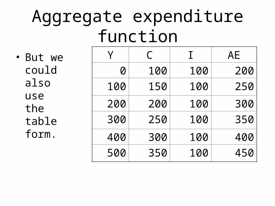
• But we could also use the table form.

Y C I AE

0 100 100 200

100 150 100 250

200 200 100 300

300 250 100 350

400 300 100 400

500 350 100 450

Equilibrium in two sector model

• Equilibrium in a model is a situation of “balance”. In our AE model, equilibrium requires that demand for goods (AE) is equal to supply of goods (Y).Y = AE = C + I

• For the equilibrium we are looking for the value of GDP, Y*, such that goods demand and goods supply are equal.

• In our two sector AE model that means that we can look up our AE table and find where AE = Y.

• The equilibrium value of Y will be our prediction of GDP for our AE model.

Equilibrium

• The equilibrium value of GDP is $400bn.

Y C I AE

0 100 100 200

100 150 100 250

200 200 100 300

300 250 100 350

400* 300 100 400*

500 350 100 450

Equilibrium

• We could accomplish the same by using our graph of the AE function.– The AE line shows us the level of goods

demand for each value of Y.– The 45 degree line represents the value of Y

or supply of goods.– Equilibrium will occur when the 45 degree line

and the AE line cross. At the crossing, goods demand is equal to goods supply for that level of Y.

Equilibrium

• The equilibrium value of Y is where the 45 degree line and the AE line cross. Y* is at $400bn.

Y

Y

AE = 200 + 0.5Y

400

400

Equilibrium

• Finally, if you are comfortable with the mathematics, you can solve for the equilibrium value of Y using the equations:Y* = AE = 200 + 0.5Y*Y* – 0.5Y* = 2000.5Y* = 200Y* = 400

• You arrive at the same answer no matter which way you use to derive it.

Autonomous expenditure

• In our model we have two part of aggregate expenditure:AE = $200bn + 0.5Y– One part does not depend on the value of Y-

the $200bn. This portion is called “autonomous expenditure”.

– The other part does depend on the value of Y- the 0.5Y.

• In our model part of autonomous expenditure is C and part is I.

Scenario: Investment falls

• What happens if I drops from 100 to 50 perhaps because of uncertainty due to terrorism scares?

• Equilibrium GDP drops to 300.

Y C I AE

0 100 50 150

100 150 50 200

200 200 50 250

300* 250 50 300*

400 300 50 350

500 350 50 400

Scenario

• But you could also find the same answer with some algebra:AE = C + I = 100 + 0.5Y + 50 = 150 + 0.5YY* = AE = 150 + 0.5Y*Y* – 0.5Y* = 1500.5Y* = 150Y* = 300

• Find the answer in the way you feel most comfortable.

Multiplier

• So a $50bn drop in investment (or autonomous expenditure) leads to a $100bn drop in equilibrium GDP.

• The ratio of the change in GDP over the change in autonomous expenditure is called the multiplier:Multiplier = (Change in GDP)/(Change in I)

Expenditure multiplier

• Imagine the government wishes to affect the economy. One tool available is government consumption, G, or government taxes, T. This is called “fiscal policy”.

• Any change in G (∆G) in our AE model will produce:

ΔGmpc-1

1 ΔY

Multiplier

• If mpc=0.75, then the multiplier is (1/0.25) or 4, so $1 of new G will produce $4 of new Y.

• Our multiplier is equal to 1/(1-MPC).

• Since 0<MPC<1, our multiplier will be greater than 1.

• The larger is the MPC, the larger is our multiplier.

Three sector AE model

• Now we make our model slightly more complicated by bringing in the government. The government has two effects on our model:– The government raises tax revenues (T) by taxing

household incomes.– The government purchases some goods and services

for government consumption (G).

• We treat the levels of T and G as exogenous to our AE model. Government policy determines what T and G will be, and policy is not affected by the equilibrium level of GDP.

Three sector model

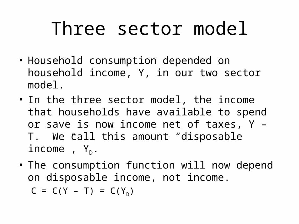
• Household consumption depended on household income, Y, in our two sector model.

• In the three sector model, the income that households have available to spend or save is now income net of taxes, Y – T. We call this amount “disposable income”, YD.

• The consumption function will now depend on disposable income, not income.C = C(Y – T) = C(YD)

Three sector model

• Our new aggregate expenditure function includes government purchases of goods and services, so we have:AE = C + I + G

• Let’s assume we have the same linear consumption function as before, but now in disposable income:C = 100 + 0.5 (Y – T)

• Let T = G = 50 and let I = 100. We can follow the same steps as before to find our AE function and then to find equilibrium GDP.

Aggregate expenditure function

• Our AE function is:AE = C(Y – T) + I + G

AE = 100 + 0.5(Y – 50) + 100 + 50

AE = 100 + 0.5Y – 25 + 100 + 50

AE = 225 + 0.5Y

• We can also represent this as a table. Our C function with disposable income is:C = 100 + 0.5(Y-50) = 75 + 0.5Y

Table form

Y C = 75 + 0.5Y

I G AE

0 75 100 50 225

100 125 100 50 275

200 175 100 50 325

300 225 100 50 375

400 275 100 50 425

500 325 100 50 475

Equilibrium

• If we want to find equilibrium GDP in our three sector model, we need to find the level of GDP, Y*, for which goods demand (AE) is equal to goods supply (Y).

• If we look at our table, we see that for an income level of Y of 400, AE is 425 which exceeds Y. At an income level of Y of 500, AE is 475 which is less than Y.

• We would guess that the equilibrium value of Y lies between 400 and 500.

• We construct a new table of values of Y between 400 and 500.

Equilibrium

Y C = 75 + 0.5Y

I G AE

400 275 100 50 425

425 287.5 100 50 437.5

450* 300 100 50 450*

475 312.5 100 50 462.5

500 325 100 50 475

Equilibrium

• The equilibrium value of Y is 450.

• We could find the answer with our equations:AE = 225 + 0.5Y

Y* = AE = 225 + 0.5Y*

Y* - 0.5Y* = 225

0.5Y* = 225

Y* = 450

Scenario: Investment falls

• What happens if we have the same drop in investment in the three sector model? So I drops from 100 to 50?

• Using our equations:AE = 100 + 0.5(Y - T) + I + GAE = 75 + 0.5Y + 50 + 50AE = 175 + 0.5Y

• Solving for Y*, we get:Y* = AE = 175 + 0.5Y*Y* = 350

• Our multiplier = 100/50 = 2 as before.

Deriving aggregate demand

• How do average prices affect demand for goods and services?– Real balances effect: higher prices means our assets have less

value so people are poorer and consume less.– Interest-rate effect: higher prices drive up the demand for

money and so drive up interest rates, at higher interest rates, investment falls (see later)

– Foreign-purchases exports: at higher Australian prices, foreign goods are cheaper, so net exports falls (see later)

• As the average price level rises, demand for goods and services should fall, with all else held constant.

Deriving AD

• So as P↑, we expect:– C↓ (real balances)– I↓ (interest rate)– NX↓ (foreign-

purchases)

• So as P↑, we expect:AE = C↓ + I↓ + G + NX↓

• The AE curve shifts down.

• Equilibrium Y* falls.

Aggregate demand

• We would like to have a relationship between the demand for goods and services and the price level. We call this the “aggregate demand” (AD) curve.

• The AD curve is downward-sloping in aggregate price.

Y

P0

Y0 Y1

P1

AD

Shifts of the AD curve

• Factors that affect the AE curve will affect the AD curve. For example, if household wealth rose, then C would increase for all levels of disposable income. Demand would be higher for all levels of prices, so the AD curve shifts to the right.– C: household wealth, household expectations about

the future– I: interest rates, business expectation about the

future, technology– G and T: changes in fiscal policy– NX: the currency exchange rate, change in output in

foreign countries

AD and the multiplier

• A change in I will shift the AE curve up. This will produce a shift to the right of the AD curve.

• The shift in the AD curve will be the change in I times the multiplier.

Aggregate supply

• The aggregate demand curve showed the relationship between goods demand and the average level of prices.

• The aggregate supply (AS) curve shows the relationship between goods supply and the average level of prices.

• By goods supply, we are thinking about all of the goods and services provided by all the producers in the economy.

• How does the aggregate price level affect the aggregate level of goods and services supply?

Deriving the AS curve

• We will differentiate between goods supply in the short-run (SR) and in the long-run (LR).

• The crucial difference between the two time periods is that we will assume that nominal wages for employees are fixed in the SR. Workers’ money wages do not change in the SR. But workers’ wages are free to move in the LR.

• So we will have two different AS curves- the SR AS and the LR AS curves.

Fixed nominal wages

• How can we defend the assumption that wages are fixed in the SR?– All wages in a modern economy are set either via

contracts between employers and employees or via a labour agreement between unions and employers.

– These contracts specify well in advance (a few months to several years) what the wages of a worker will be in nominal terms.

– These contracts are usually very difficult to change.

Supply of an individual firm

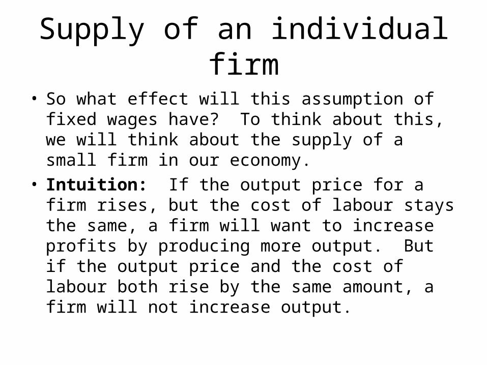
• So what effect will this assumption of fixed wages have? To think about this, we will think about the supply of a small firm in our economy.

• Intuition: If the output price for a firm rises, but the cost of labour stays the same, a firm will want to increase profits by producing more output. But if the output price and the cost of labour both rise by the same amount, a firm will not increase output.

Deriving the SR AS curve

• In the short-run (“SR”), since wages are fixed, a rise in P will have no affect on W, so individual firms will find it profitable to increase output.

• As all firms are raising output, aggregate supply will increase in the SR if aggregate prices rise.

• So the SR AS curve is upward-sloping in aggregate prices.

Deriving the LR AS curve

• We assume that workers are interested in their real wages (wages relative to prices W/P).

• If P rises, workers will demand a compensating W rise, so as to keep real wages the same as before.

• In the LR, real wages are unchanged by changes in P, so output is not affected by changes in P.

• The LR AS curve is vertical at the “natural rate of output”.

The LR AS curve

• The LR AS curve is vertical, so long-run Y does not depend on prices.

• The long-run Y is determined by:– Labour skills– Capital efficiency– Technology– Labour market rules– And others…

YYLR

LR ASP

Low U/E

HighU/E

Review: Aggregate supply

• There will be a short-run AS curve which is upward-sloping in prices.

• The SR AS (or usually just “AS”) is used to model scenarios.

• The long-run AS curve is vertical at the level of potential output, since wages will change proportionately to price changes.

• The LR AS is used (mostly) to talk about unemployment.

Equilibrium

• Equilibrium occurs at a price level where goods demand (AD) is equal to goods supply (SR AS).

YY0

P0

AD

AS

P

Unemployment

• The gap between the “natural rate of output” and current output is called the “recessionary gap”.

• The level of unemployment depends on the size of this gap.YY0

P0

AD

AS

PLR AS

YLR

Unemployment

Shift in AD (C↑ or G↑ or T↓ or I↑ or NX↑)

Shift in AD

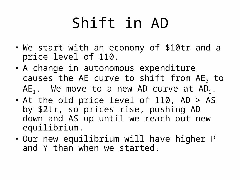
• We start with an economy of $10tr and a price level of 110.

• A change in autonomous expenditure causes the AE curve to shift from AE0 to AE1. We move to a new AD curve at AD1.

• At the old price level of 110, AD > AS by $2tr, so prices rise, pushing AD down and AS up until we reach out new equilibrium.

• Our new equilibrium will have higher P and Y than when we started.

Shift in AD

Shift in AS (rise in oil prices)

• A rise in oil prices raises the cost of production for all producers and shifts the SR AS curve up/to the left.

• At the old prices, AD > AS, so prices rise and output falls.YY1

P0

AD

AS1

P

AS0

Y0

P1

Business cycle

• Over the business cycle, we will have periods of high output (booms) and periods of low output (recessions).

• In booms, output is high and unemployment is low, while in recessions, output is low and unemployment is high.

• The “natural rate of unemployment” is the level of unemployment in a “normal” period of the economy. This is achieved when output is at full-employment or the LR AS level.

A “Boom” in the Economy

• An economy in a boom is an economy with an output level higher than the natural rate of output.

• Unemployment is below the natural rate in a boom.

YY0

P0

AD

AS

PLR AS

YLR

A “Recession”

• An economy in a recession is an economy with an output level below the natural rate of output.

• Unemployment is above the natural rate in a recession.

YY0

P0

AD

AS

PLR AS

YLR

Sample AD-AS question

• The small country of Speckonamap is in long-run equilibrium with its aggregate demand (AD) and short-run aggregate supply (AS) curves intersecting on the long-run aggregate supply curve (ASLR). The dot-com bubble in Speckonmap’s industry bursts. Business investment drops.

• a. Explain the short- and long-term consequences of this bursting bubble using the AD-AS diagram. Be as clear and complete as you can.

Sample AD-AS question

• b. What policies could the government of Speckonamap pursue to counter the collapse of business investment? Think of two different ways that the government could shift the AD-AS curves.

Investment

• Investment can refer to the purchase of new goods that are used for future production. Investment can come in the form of machines, buildings, roads or bridges. This is called “physical capital”.

• Another type of investment is called “human capital”. This is investment in education, training and job skills.

• Usually when we talk about investment, we mean investment in physical capital, but investment should include all forms of capital.

Investment decision-making

• How to determine profitability of investment?• Example: An investment involves the current

cost of investment (I). The investment will pay off with some flow of expected future profits. The future stream of profits is R1 in one year’s time, R2 in two year’s time, … up to Rn at the nth year when the investment ends.

• Net Present Value (NPV) = Present Value of Future Profits (PV) – Investment (I)

Investment decision-making

• What determines investment?– Businesses or individuals make an investment if they

expect the investment to be profitable.

• Imagine we have a small business owner who is faced with an investment decision.

• The small business owner will make the investment as long as the investment is profitable.

• How to determine profitability of investment?

Profitability of an investment

• Example: – An investment involves the current cost of investment (I). – The investment will pay off with some flow of expected future

profits. – The future stream of profits is R1 in one year’s time, R2 in two

year’s time, … up to Rn at the nth year when the investment ends.

• Imagine you are the business owner. How do we decide whether to make the investment? Can we simply add up the benefits (profits) and subtract the costs (investment)?

Profits today = R1 + R2 + … + Rn – I?

• What is wrong with this calculation?

Present value concept

• Imagine our rule about future values was simply to add future costs and benefits to costs and benefits today.

• Scenario: A friend offers you a deal: – “Give me $10 today, and I promise to give you $20 in 1 years

time.”• If we subtract costs ($10) from benefits ($20), we get a

positive value of $10. Does this seem like a sensible decision?

• Scenario: A friend offers you a deal: – “Give me $10 today, and I promise to give you $20 in 100 years

time.”• If we subtract costs ($10) from benefits ($20), we get a

positive value of $10. Does this seem like a sensible decision?

Present value concept

• Not really. The problem is that a $1 today is not the same as a $1 in a year’s time or 100 years’ time.

• We can not directly add these $1s together since they are not the same things. We are adding apples and oranges.

• We need a way of translating future $1s into $1s today, so that we can add the benefits and costs together.

• The conversion is called “present value”. • In making the decision about our friend’s deal, we would

compare $10 today to the present value of the $20 in a year or 100 years.

Present value concept

• An investment is about giving up something today in order to get back something in the future.

• So an investment decision will always involve comparing $1s today to $1s in the future.

• Investment decisions will always involve present values. If we subtract the present value of future profits from costs today, we get net present value.Net Present Value (NPV) = Present Value of Future

Profits (PV) – Investment (I)

Net present value

• The investment rule will be to invest if and only if:

NPV ≥ 0

• Or

Present Value of Future Profits (PV) – Investment (I) ≥ 0

Interest rates

• Interest rates are a general term for the percentage return on a dollar for a year:– that you earn from banks for saving– that you pay banks for borrowing or investing

• For example, the interest rate might be 10%, so if you put $1 in the bank this year, it will become $(1+i) in one year’s time.

• Or if you borrow $100 today, you will have to repay $(1+i)100 next year.

Interest Rates

0.00

2.00

4.00

6.00

8.00

10.00

12.00

14.00

16.00

18.00

Jan-

70

Jan-

73

Jan-

76

Jan-

79

Jan-

82

Jan-

85

Jan-

88

Jan-

91

Jan-

94

Jan-

97

Jan-

00

Jan-

03

Bank Interest Rates

Discounting future values

• How do we place a value today on $1 in t years’ time?

• This is called “discounting” the future value. One way to think about this question is to ask:– “How much would we have to put in the bank now to

have $1 in t years’ time?”– Money in the bank earns interest at the rate at the

rate i, i>0. If I put $1 in the bank today, it will grow to be $(1+ i)1 in one year’s time, will grow to be $(1+i)(1+i)1 = $(1+i)2 in two years’ time and will grow to $(1+i)n in n years’ time.

Bank account

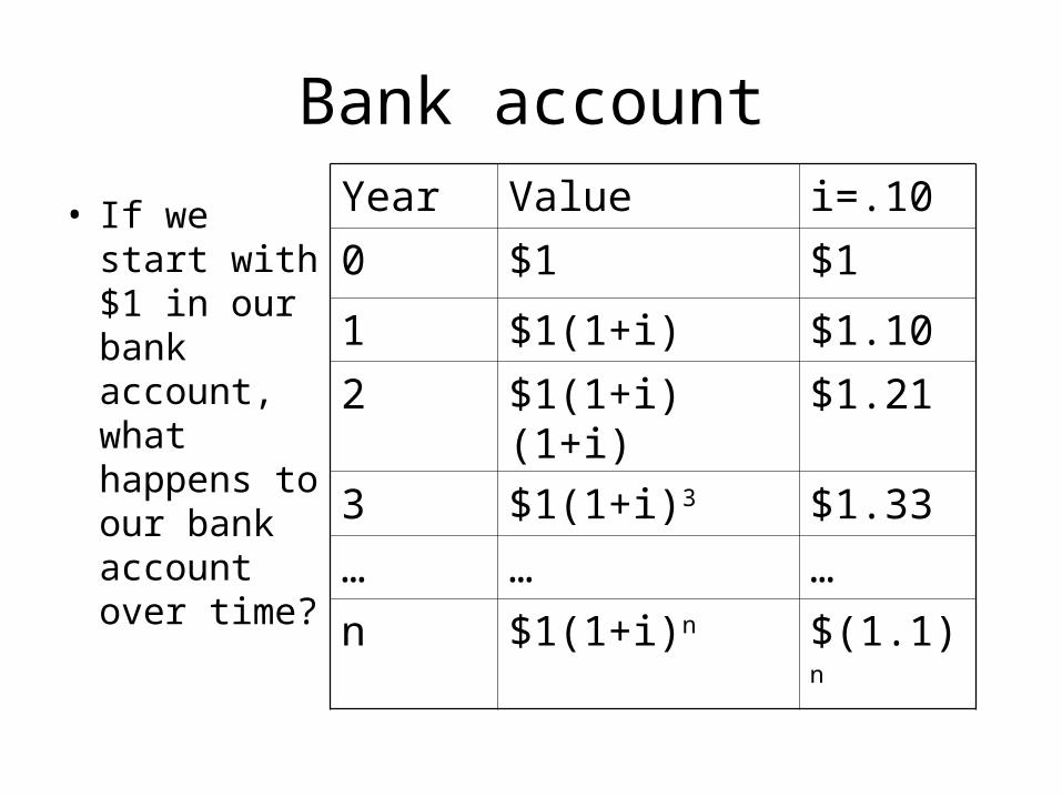
• If we start with $1 in our bank account, what happens to our bank account over time?

Year Value i=.10

0 $1 $1

1 $1(1+i) $1.10

2 $1(1+i)(1+i) $1.21

3 $1(1+i)3 $1.33

… … …

n $1(1+i)n $(1.1)n

How much is a future $1?

• In order to have $1 next year, we would have to put x in today:

$1 = (1+ i) $x$x = 1/(1+i) < 1

• $1 next year is worth 1/(1 + i) today. Since i>0, $1 next year is worth less than $1 today.

• In order to have $1 in n years’ time, we would have to put x in today:

x = 1/(1+i)n = (1+i)-n

• $1 in n years’ time is worth 1/(1+i)n < 1 today.

PV of $1

Year i=0.01 i=0.05 i=0.10 i=0.20

0 1 1 1 1

1 0.99 0.95 0.91 0.83

2 0.98 0.91 0.83 0.69

3 0.97 0.86 0.75 0.58

10 0.91 0.61 0.39 0.16

n (1.01)-n (1.05)-n (1.10)-n (1.20)-n

Net present value

• NPV = R1/(1+i) + R2/(1+ i)2 + … + Rn/(1+ i)n – I• If NPV >=0, then go ahead and make the

investment. If NPV < 0, then the investment is not worthwhile.

• As i rises, the PV of future profits will drop, so the NPV will fall. If we imagine that there are thousands of potential investments to be made, as i rises, fewer of these potential investments will be profitable, and so investment will fall.

• We expect then that I falls as i rises.

Investment decision

• Imagine we are the small business owner we were discussing before. We have a new project which we might invest in:– An investment involves the current cost of

investment (I). – The investment will pay off with some flow of

expected future profits. – The future stream of profits is R1 in one year’s

time, R2 in two year’s time, … up to Rn at the nth year when the investment ends.

Investment decision

Year Benefit Cost PV

0 0 I -I

1 R1 0 R1/(1+i)

2 R2 0 R2/(1+i)2

3 R3 0 R3/(1+i)3

… … … …

n Rn 0 Rn/(1+i)n

Net present value

• The NPV of the investment is the sum of the values in the far-right column- the PVs.NPV = R1/(1+i) + R2/(1+ i)2 + … + Rn/(1+ i)n – I

• If NPV ≥ 0, then go ahead and make the investment. If NPV < 0, then the investment is not worthwhile.

• Let’s look at a more concrete example that we can put some numbers to.

Example of NPV

• Example: A small business in Bathurst that owns photo store is considering installing a state-of-the-art developing machine for digital photographs.– Cost = $12,000 (after selling current machine)– Future benefits = $2,000 per year in extra

business every year for 10 year life-span of machine (assume benefits start next year)

Example of NPV

Year Benefit Cost PV

0 0 I -$12,000

1 $2,000 0 $2,000/(1+i)

2 $2,000 0 $2,000/(1+i)2

3 $2,000 0 $2,000/(1+i)3

… … … …

10 $2,000 0 $2,000/(1+i)10

Example of NPV

• NPV = -$12,000 + $2,000/(1+i) + $2,000/(1+i)2 + $2,000/(1+i)3 + … + $2,000/(1+i)10

• Our NPV then depends upon the interest rate, i, facing the small business.

• For a small business, the relevant interest rate would be the rate that it cost raise the money, say by taking out a bank loan.

• So the interest rate would be the bank small business loan rate.

Example of NPV

• The NPV varies with the interest rate:– At i=0.05, NPV = $3,443, so go ahead with

investment.– At i=0.08, NPV = $1,420, so go ahead with

investment.– At i=0.10, NPV = $289, so go ahead with investment.– At i=0.12, NPV = -$700, so don’t go ahead with the

investment.

• Somewhere between a 10% and a 12% interest rate, NPV = 0. NPV < 0 for all interest rates greater than 12%.

Example of NPV

• Another way of thinking about this problem is to ask “Can I repay the loan and still make money?”

• The small business owner borrows $12,000 from the bank and uses the $2,000 in extra business each year to repay the loan.

• Would the business owner repay the loan before the machine needs to be replaced?

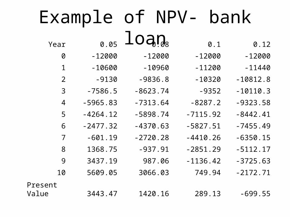
Example of NPV- bank loanYear 0.05 0.08 0.1 0.12

0 -12000 -12000 -12000 -12000

1 -10600 -10960 -11200 -11440

2 -9130 -9836.8 -10320 -10812.8

3 -7586.5 -8623.74 -9352 -10110.3

4 -5965.83 -7313.64 -8287.2 -9323.58

5 -4264.12 -5898.74 -7115.92 -8442.41

6 -2477.32 -4370.63 -5827.51 -7455.49

7 -601.19 -2720.28 -4410.26 -6350.15

8 1368.75 -937.91 -2851.29 -5112.17

9 3437.19 987.06 -1136.42 -3725.63

10 5609.05 3066.03 749.94 -2172.71

Present Value 3443.47 1420.16 289.13 -699.55

Example of a NPV- bank loan

• So for interest rates of 10% and below, the bank loan is repaid before the machine wears out, so the investment is worthwhile.

• For interest rates of 12% and above, the bank loan is not repaid by the time the machine needs to be replaced, so the investment is not worthwhile.

• The bottom line shows that the remainder in the bank account at the end of 10 years is the NPV of the investment decision.

• So another way to think of NPV is as the money left in an account at the end of a project.

Investment demand

• Instead of thinking about a single small business, think of a whole economy of businesses and individuals making investment decisions.

• Some of these investment decisions will be very good ones and some will be very poor ones. There is a whole range.

• As i rises, the PV of future profits will drop, so the NPV will fall. If we imagine that there are thousands of potential investments to be made, as i rises, fewer of these potential investments will be profitable, and so investment will fall.

Investment demand

• If we graphed the investment demand for goods and services (I) against interest rates, it would be downward-sloping in i. The higher is i, the lower is investment demand.

• What can shift the I curve? Factors that affect current and expected future profitability of projects:– New technology– Business expectations– Business taxes and regulation

Shifts in investment demand

• Example: An increase in business confidence/expectations raises the expected future profits for businesses.

• At the same interest rates as before, since the Rs are higher, the NPVs of all investment projects will be higher.

• The investment demand curve is shifted to the right. I is higher for all interest rates.

Uses of PV concept

• Housing valuation: We can use the PV concept to estimate what house prices should be.

• What do you have when you own a home? You have the future housing services of that home plus the right to sell the home.

• Value of housing services should be the price people pay to rent an equivalent home. Rent is the price of a week of housing services.

• Let’s say your home rents for $250 per week.

Housing valuation

• If you stayed in your home for 50+ years, your house is worth the PV of 50 years of 52 weekly $250 payments plus any sale value at 50 years. How do we calculate the PV of such a long stream of numbers?

• Trick: For very long streams, the sum:• PV = ($250 x 52) + ($250 x 52)/(1+i) + …• Is very close to:• PV = ($250 x 52) / i = $13,000 / i

Housing valuation

• So we get the house values:– At i=0.02, PV House = $650,000– At i=0.03, PV House = $433,000– At i=0.05, PV House = $260,000– At i=0.06, PV House = $217,000– At i=0.07, PV House = $186,000

• At a house price above this price, you are better off selling your house and renting for 50 years. At a house price below this price, you are better off owning a house.

Housing valuation

• You can also see how sensitive house prices are to the interest rate. When i rose from 6% to 7%, the value of the house dropped $31,000.

• You can see why home owners care so much about the home loans rates.

• But what about the resale price at 50 years? – The PV of the house sale in 50 years time is (Sale

Price) / (1+i)50, which for most values of i is going to be a very small number- 8% of Sale Price at 5% interest and 3% of Sale Price at 7% interest.

Housing price bubbles

• Sometimes the price of housing can vary from this PV of housing services price. Some analysts argue that today’s housing prices is one case- these periods are called “bubbles”.

• Example: At 6% interest rates our house was worth $217,000. Let’s say Sam bought the house for $300,000 in order to sell the house one year from now.

• In order to be able to repay the $300,000, Sam has to gain $18,000 (6% of $300,000) by holding the house for a year.

Housing price bubbles

• Since Sam gets $13,000 worth of housing services from the house, the value of the house has to rise $5,000 to $305,000 in next year’s sale for a total gain of $18,000.

• Even though the house is unchanged, the “overpayment” for the house has to rise- the house is still only worth $217,000 in housing services- but it now sells for $305,000.

• So in a “bubble”, if people are overpaying for a house, the overpayment has to keep rising. Eventually people realize that the house only generates $217,000 in services.

Housing price bubbles

• Example: In Holland in 1636, the price of some rare and exotic tulip bulbs rose to the equivalent of a price of an expensive house. People paid that much in plans to resell at even higher prices.

• In 1637, prices for tulips crashed and by 1639, tulip bulbs were selling for 1/200th of the peak prices.

• Bubbles tend to crash fast and dramatically.

Example: Bond Valuation

You can save money at the bank and earn a 10% yearly return on your savings. What is the most you would be willing to pay for (include your calculations and explain carefully):

a. a promise of a $1 in one year’s time (assume that this promise will not be broken);

Example question

b. a 10 year $100 savings bond (the bond will pay you $100 in the year 2015, where 2015 is known as the ‘maturity date’) and do a graph of the value of the 10 year $100 maturity in 2015 savings bond as we get closer to the maturity date; and

Example question

c. a 10 year $100 savings bond that also pays you $5 per year for every year that you hold the bond (including the 10th year).

Resources

• There are many resources available to you. Often students hurt themselves by not taking advantage of the resources they have.

• Books: There are plenty of macroeconomics principles books. If you don’t understand Jackson and McIver’s coverage, get to a library and read a different textbook. There is also a study guide by Bredon and Curnow referenced in the subject outline.

• Online: There is an enormous amount of material on the Web. Just use a search engine and look around.

Resources

• Forum: Get into a habit of reading the CSU forums once a week. Post questions on the forum and join in the discussion.

• Official websites: Have a look at the websites for government agencies like the Reserve Bank of Australia or the Australian Bureau of Statistics.

• CSU help: Student Services at CSU has a lot of help it can provide students with problems- look at http://www.csu.edu.au/division/studserv/.