École de technologie supÉrieure universitÉ du quÉbec€¦ · iv algorithmes génétiques...
TRANSCRIPT


ÉCOLE DE TECHNOLOGIE SUPÉRIEURE
UNIVERSITÉ DU QUÉBEC
A THESIS PRESENTED TO THE
ÉCOLE DE TECHNOLOGIE SUPÉRIEURE
IN FULLFILMENT OF THE THESIS REQUIREMENT
FOR THE DEGREE OF
PHILOSOPHIAE DOCTOR IN ENGINEERING
Ph.D.
BY
PAULO VINICIUS WOLSKI RADTKE
CLASSIFICATION SYSTEMS OPTIMIZATION
WITH MULTI-OBJECTIVE EVOLUTIONARY ALGORITHMS
MONTRÉAL, SEPTEMBER 14, 2006
© copyrights reserved by Paulo Vinicius Wolski Radtke

THIS THESIS WAS EVALUATED
BY A COMMITTEE COMPOSED BY :
Mr. Robert Sabourin, thesis supervisor Département de génie de la production automatisée at École de technologie supérieure Mr. Tony Wong, thesis co-supervisor Département de génie de la production automatisée at École de technologie supérieure Mr. Richard Lepage, president Département de génie de la production automatisée at École de technologie supérieure Mr. Mohamed Cheriet, examiner Département de génie de la production automatisée at École de technologie supérieure Mr. Marc Parizeau, external examiner Département de génie électrique et de génie informatique at Université Laval
THIS THESIS WAS DEFENDED IN FRONT OF THE EXAMINATION
COMMITTEE AND THE PUBLIC
ON SEPTEMBER 11, 2006
AT THE ÉCOLE DE TECHNOLOGIE SUPÉRIEURE

CLASSIFICATION SYSTEMS OPTIMIZATION WITH MULTI-OBJECTIVE EVOLUTIONARY ALGORITHMS
Paulo Vinicius Wolski Radtke
ABSTRACT
The optimization of classification systems is a non-trivial task, which is most of the time performed by a human expert. The task usually requires the application of domain knowledge to extract meaningful information for the classification stage. Feature extraction is traditionally a trial and error process, where the expert chooses a set of candidate solutions to investigate their accuracy, and decide if they should be further refined or if a solution is suitable for the classification stage. Once a representation is chosen, its complexity may be reduced through feature subset selection (FSS) to reduce classification time. A recent trend is to combine several classifiers into ensemble of classifiers (EoC), in order to improve accuracy. This thesis proposes a feature extraction based approach to optimize classification systems using a multi-objective genetic algorithm (MOGA). The approach first optimizes feature sets (representations) using the Intelligent Feature Extractor (IFE) methodology, selecting from the resulting set the best representation for a single-classifier based system. After this stage, the selected single classifier can have its complexity reduced through FSS. Another approach is to use the entire IFE result set to optimize an EoC for higher classification accuracy. Classification systems optimization is challenged by the solution over-fit to the data-set used through the optimization process. This thesis also details a global validation strategy to control over-fit, based on the validation procedure used during classifier training. The global validation strategy is compared to traditional methods with the proposed approach to optimize classification system. Finally, a stopping criterion based on the approximation set improvement is also proposed and tested in the global validation context. The goal is to monitor algorithm improvement and stop the optimization process when it cannot further improve solutions. An experiment set is performed on isolated handwritten digits with two MOGAs, the Fast Elitist Non-Dominated Sorting Algorithm (NSGA-II) and the Multi-Objective Memetic Algorithm (MOMA). Both algorithms are compared to verify which is the most appropriate for each optimization stage. Experimental results demonstrate that the approach to optimize classification systems is able to outperform the traditional approach in this problem. Results also confirm both the global validation strategy and the stop criterion. The next experiment set uses the best configuration found with digits

ii
to optimize isolated uppercase handwritten letters, demonstrating the approach effectiveness on an unknown problem.

OPTIMISATION DES SYSTÈMES DE CLASSIFICATION AVEC ALGORITHMES ÉVOLUTIFS MULTICRITÈRE
Paulo Vinicius Wolski Radtke
SOMMAIRE
L’optimisation des systèmes de classification est une tâche complexe qui requiert l’intervention d’un spécialiste (expérimentateur). Cette tâche exige une bonne connaissance du domaine d’application afin de réaliser l’extraction de l’information pertinente pour la mise en œuvre du système de classification ou de reconnaissance. L’extraction de caractéristiques est un processus itératif basé sur l’expérience. Normalement plusieurs évaluations de la performance en généralisation du système de reconnaissance, sur une base de données représentative du problème réel, sont requises pour trouver l’espace de représentation adéquat. Le processus d’extraction de caractéristiques est normalement suivi par une étape de sélection des caractéristiques pertinentes (FSS). L’objectif poursuivi est de réduire la complexité du système de reconnaissance tout en maintenant la performance en généralisation du système. Enfin, si le processus d’extraction de caractéristiques permet la génération de plusieurs représentations du problème, alors il est possible d’obtenir un gain en performance en combinant plusieurs classificateurs basés sur des représentations complémentaires. L’ensemble de classificateurs (EoC) permet éventuellement une meilleure performance en généralisation pour le système de reconnaissance. Nous proposons dans cette thèse une approche globale pour l’automatisation des tâches d’extraction, de sélection de caractéristiques et de sélection des ensembles de classificateurs basés sur l’optimisation multicritère. L’approche proposée est modulaire et celle-ci permet l’intégration de l’expertise de l’expérimentateur dans le processus d’optimisation. Deux algorithmes génétiques pour l’optimisation multicritère ont été évalués, le Fast Elitist Non-Dominated sorting Algorithm (NSGA-II) et le Multi-Objective Memetic Algorithm (MOMA). Les algorithmes d’optimisation ont été validés sur un problème difficile, soit la reconnaissance de chiffres manuscrits isolés tirés de la base NIST SD19. Ensuite, notre méthode a été utilisée une seule fois sur un problème de reconnaissance de lettres manuscrites, un problème de reconnaissance provenant du même domaine, pour lequel nous n’avons pas développé une grande expertise. Les résultats expérimentaux sont concluants et ceux-ci ont permis de démontrer que la performance obtenue dépasse celle de l’expérimentateur. Finalement, une contribution très importante de cette thèse réside dans la mise au point d’une méthode qui permet de visualiser et de contrôler le sur-apprentissage relié aux

iv
algorithmes génétiques utilisés pour l’optimisation des systèmes de reconnaissance. Les résultats expérimentaux révèlent que tous les problèmes d’optimisation etudiés (extraction et sélection de caractéristiques de même que la sélection de classificateurs) souffrent éventuellement du problème de sur-apprentissage. À ce jour, cet aspect n’a pas été traité de façon satisfaisante dans la littérature et nous avons proposé une solution efficace pour contribuer à la solution de ce problème d’apprentissage.

OPTIMISATION DES SYSTÈMES DE CLASSIFICATION AVEC ALGORITHMES ÉVOLUTIFS MULTICRITÈRE
Paulo Vinicius Wolski Radtke
RÉSUMÉ
Le processus d’extraction de caractéristiques est un processus qui relève de la science de l’expérimentateur. C’est un processus très coûteux et qui repose également sur l’habileté de l’expérimentateur, à la fois sur son expertise et sur sa connaissance du domaine d’application. Nous avons abordé le processus d’extraction de caractéristiques comme un problème d’optimisation multicritère (MOOP). La méthode proposée est modulaire, ce qui permet de diviser le problème d’optimisation des systèmes de reconnaissance en trois sous-problèmes: l’extraction de caractéristiques, la sélection de caractéristiques pertinentes et enfin la sélection des classificateurs dans les ensembles de classificateurs (EoC). L’intérêt des algorithmes évolutionnaires pour l’optimisation des systèmes de recon-naissance de formes est qu’ils représentent des algorithmes de recherche stochastiques basés sur l’évolution d’une population de solutions (eg de représentations, de classificateurs, etc.). Un avantage immédiat d’avoir une population de solutions est de considérer les N meilleures solutions pour la mise en œuvre du système de reconnaissance. Ce type d’approche est habituellement plus robuste et permet une meilleure performance en généralisation sur des données qui n’ont pas été utilisées lors de la conception du système. De plus, les algorithmes évolutionnaires utilisés pour l’optimisation ne requièrent pas une fonction objectif dérivable et la population de solutions permet de s’affranchir des minima locaux. Un autre avantage des algorithmes d’optimisation multicritère réside dans la facilité d’adaptation de ces algorithmes pour une gamme très grande de problèmes d’optimisation différents. En effet, l’expérimentateur n’est plus obligé de choisir a priori la valeur des coefficients de pondération des objectifs et peut attendre à la fin du processus d’optimisation pour effectuer un choix définitif à partir de l’analyse des solutions optimales qui sont inclus dans Front de Pareto (FP). Cette approche réduit au minimum l’intervention humaine dans le processus d’optimisation. L’objectif principal de cette thèse est de formaliser les processus d’extraction, de sélection de caractéristiques et de génération d’ensembles de classificateurs comme un problème d’optimisation à plusieurs niveaux. Une approche modulaire a donc été proposée où un algorithme d’optimisation multicritère a été utilisé pour résoudre chaque sous-problème.

vi
Le premier chapitre présente l’état de l’art dans les domaines qui touchent de près l’élaboration de cette thèse. En effet, une des difficultés de ce travail de recherche est qu’il se situe à la frontière de plusieurs domaines de recherche : la reconnaissance de formes en général et la reconnaissance de chiffres manuscrits en particulier, les algorithmes d’optimisation évolutionnaires multicritère, l’extraction de caractéristiques pertinentes, la sélection de caractéristiques et enfin la sélection des ensembles de classificateurs. La méthode globale retenue pour l’optimisation des systèmes de classification est exposée au chapitre deux. L’extraction des caractéristiques repose sur une technique de zonage souvent utilisée dans le domaine de la reconnaissance de caractères manuscrits isolés. Deux opérateurs de division de l’image en différentes configurations de zones sont proposés. Ensuite le lien entre le processus d’extraction et ceux associés à la sélection des caractéristiques et des classificateurs est ensuite présenté. Une contribution importante est discutée au chapitre trois. Une analyse détaillée du comportement de l’algorithme NSGA-II appliquée à l’optimisation du processus d’extraction de caractéristiques a permis de soulever les lacunes de ce type d’algorithme utilisé pour l’optimisation des systèmes de reconnaissance. Afin de combler ces lacunes, nous avons proposé un algorithme mieux adapté pour optimiser les machines d’apprentissage, soit le Multi-Objective Memetic Algorithm (MOMA). Celui-ci combine un MOGA traditionnel avec un algorithme de recherche local pour augmenter la diversité des solutions dans la population. Ce type de méthodes hybrides utilisées pour l’optimisation multicritère permet aux algorithmes évolutionnaires traditionnels de s’affranchir du problème chronique de la convergence prématurée en favorisant à la fois l’exploration et l’exploitation de nouvelles solutions. Le chapitre quatre propose une méthode innovante pour s’affranchir du problème très important du sur-apprentissage. En effet, il n’y a pas de travaux dans la littérature qui portent spécifiquement sur le problème du sur-apprentissage relié aux algorithmes évolutionnaires utilisés pour l’optimisation de machines d’apprentissage (eg des systèmes de classification). Nous avons proposé une méthode de validation globale basée sur un mécanisme d’archivage des meilleures solutions qui permet à tous les algorithmes évolutionnaires de contrôler le sur-apprentissage. Nous avons validé les algorithmes NSGA-II et MOMA sur les problèmes d’extraction de caractéristiques (IFE), de sélection de caractéristiques (FSS) et sur celui de la sélection de classificateurs (EoC) et le tout sur deux problèmes importants, soit la reconnaissance de chiffres manuscrits isolés et sur celui de la reconnaissance des lettres majuscules. Les données proviennent d’une base de données standard – NIST SD19. Afin de réduire le coût computationnel de la méthode proposée, nous avons présenté au Chapitre 5 un critère d’arrêt basé sur l’évolution des meilleures solutions (le front de Pareto dans le cas du NSGA-II et les solutions localisées à la frontière de l’espace de recherche dans le cas du MOMA) trouvées par les algorithmes évolutionnaires durant

vii
l’évolution des populations sur plusieurs générations. Le critère proposé permet d’assurer à l’expérimentateur que les paramètres des algorithmes évolutionnaires sont bien calibrés, ce qui permet à l’algorithme de produire des solutions de meilleure qualité, et également de diminuer de façon substantielle le coût computationnel des processus IFE, FSS et EoC. Les processus IFE, FSS et EoC ont été évalués au chapitre six sur le problème de la reconnaissance de chiffres manuscrits. Les performances obtenues permettent de confirmer la supériorité de l’approche proposée par rapport à la méthodologie traditionnelle qui repose uniquement sur l’expertise de l’expérimentateur. De plus, nous avons confirmé la nécessité de contrôler le sur-apprentissage pour l’optimisation des trois sous-problèmes IFE, FSS et EoC. Enfin, nous avons utilisé notre méthode d’optimisation pour l’optimisation d’un système de reconnaissance de lettres manuscrites. En effet, notre hypothèse de départ était de mettre en œuvre une méthodologie qui permet à l’expert expérimentateur de procéder à moindre coût à l’extraction de caractéristiques pertinentes sur un autre problème de reconnaissance pour lequel il n’a pas un grand niveau d’expertise. Notre méthode est modulaire et celle-ci permet à l’expérimentateur d’injecter sa connaissance qu’il a du domaine (ici, la reconnaissance de caractères manuscrits isolés). Les résultats obtenus sont très prometteurs et les performances en généralisation des représentations optimisées par les processus IFE, FSS et EoC sont meilleures que la performance du système de référence conçu par l’expérimentateur. En résumé, nous avons contribué dans cette thèse à:
• Proposer une approche générique pour optimiser les systèmes de reconnaissance de caractères manuscrits isolés.
• Proposer un MOGA adapté au problème de l’optimisation des systèmes de classification.
• Proposer plusieurs stratégies de validation afin d’éviter le sur-apprentissage associé au processus d’optimisation de systèmes de classification avec MOGAs.
• Proposer et évaluer un critère d’arrêt adapté aux MOGAs. Ce critère d’arrêt est basé sur la convergence des meilleures solutions et il est adapté à la stratégie de validation globale (habituellement, l’exécution des MOGAs est limitée seulement par un nombre maximum de génération et ignore la convergence des solutions pour définir un critère d’arrêt prématuré).
• Évaluer la performance des algorithmes MOGAs dans le contexte de l’optimisation des systèmes de classification.

ACKNOWLEDGMENTS
Writing thesis acknowledgements is a multi-objective NP hard problem. Regardless of
how hard we try to solve it, we are unlikely to obtain the global optimum and eventually
forget someone in the process. Thus, I would like to say thanks to everyone that
contributed directly or indirectly to this thesis. My gratitude to you all cannot be
expressed with plain words.
First, I would like to thank my thesis supervisors, Dr. Robert Sabourin and Dr. Tony
Wong. I am indebted to their guidance, patience and support in this work. For their
comments and invaluable feedback, my thanks to the jury members, Richard Lepage,
Mohamed Cheriet and Marc Parizeau.
I also have to thank my parents, Paulo de F. Radtke and Ana R. W. Radtke, for
supporting me the last four years, especially through some difficult moments.
I would like to thank the researchers at the Laboratoire de Vision, d'Imagerie et
d'Intelligence Artificielle during the period I have stayed in Montreal. The laboratory
provided me a great environment to work and collaborate with friends. In this regard, I
would like to thank two old friends, Luiz Oliveira and Marisa Morita, who helped me a
lot when I moved to Montreal and when starting this work.

ix
Special thanks also go to Eulanda M. dos Santos, Guillaume Tremblay, Albert Ko,
Jonathan Milgram, Frédéric Grandidier, Youssef Fataicha, Alessandro Koerich, Luis da
Costa and Marcelo Kapp. I will not forget your friendship in the short time we have
worked together.
I also have to thank the Pontifical Catholic University of Parana and the CAPES -
Brazilian Government (scholarship grant BEX 2234-03/4) for their financial support.
This thesis would not have been possible without their support.
Above all, I have to express my sincere gratitude to Melissa Murillo Radtke, my best
friend and wife. Gratitude for supporting me since I was a master’s student and for
enduring with me all the hardships. Above all, for giving me our greatest joy, our son
Angelo. I dedicate to them this thesis.

TABLE OF CONTENTS
Page
ABSTRACT .....................................................................................................................i
SOMMAIRE .................................................................................................................. iii
RÉSUMÉ ....................................................................................................................v
ACKNOWLEDGMENTS ............................................................................................. viii
TABLE OF CONTENTS...................................................................................................x
LIST OF TABLES ......................................................................................................... xiii
LIST OF FIGURES .........................................................................................................xv
LIST OF ALGORITHMS............................................................................................. xxii
LIST OF ABREVIATIONS AND NOTATIONS ....................................................... xxiii
INTRODUCTION .............................................................................................................1
CHAPTER 1 STATE OF THE ART................................................................................8 1.1 State of the Art in Pattern Recognition ......................................................8
1.1.1 Character Representation ...........................................................................8 1.1.2 Zoning ......................................................................................................10 1.1.3 Isolated Character Recognition................................................................12 1.1.4 Feature Subset Selection ..........................................................................12 1.1.5 Ensemble of Classifiers............................................................................14 1.1.6 Solution Over-Fit .....................................................................................16
1.2 State of the Art in Multi-Objective Genetic Algorithms..........................17 1.2.1 Definitions................................................................................................19 1.2.2 Multi-Objective Genetic Algorithms .......................................................21 1.2.3 Parallel MOGAs.......................................................................................23 1.2.4 Performance Metrics ................................................................................24 1.2.5 Discussion ................................................................................................25
CHAPTER 2 CLASSIFICATION SYSTEMS OPTIMIZATION.................................26 2.1 System Overview .....................................................................................26 2.2 Intelligent Feature Extraction...................................................................28
2.2.1 Zoning Operators .....................................................................................30 2.2.1.1 Divider Zoning Operator..........................................................................30 2.2.1.2 Hierarchical Zoning Operator ..................................................................33
2.2.2 Feature Extraction Operator.....................................................................35 2.2.3 Candidate Solution Evaluation.................................................................37

xi
2.3 Feature Subset Selection ..........................................................................40 2.4 EoC Optimization ....................................................................................44 2.5 Optimization Algorithm Requirements....................................................45 2.6 Discussion ................................................................................................47
CHAPTER 3 MULTI-OBJECTIVE OPTIMIZATION MEMETIC ALGORITHM.....49 3.1 Algorithm Concepts .................................................................................49 3.2 Algorithm Discussion ..............................................................................51 3.3 MOMA Validation Tests with the IFE ....................................................55
3.3.1 Algorithmic Parameters ...........................................................................57 3.3.2 Validation and Tests.................................................................................57
3.4 IFE Test Results .......................................................................................59 3.5 Discussion ................................................................................................65
CHAPTER 4 VALIDATION STRATEGIES TO CONTROL SOLUTION OVER-FIT................................................................................................66
4.1 Adapting Optimization Algorithms .........................................................75 4.2 Discussion ................................................................................................78
CHAPTER 5 STOPPING CRITERION.........................................................................79 5.1 Concepts...................................................................................................79 5.2 Stopping MOGAs ....................................................................................81 5.3 Discussion ................................................................................................83
CHAPTER 6 VALIDATION EXPERIMENTS ON ISOLATED HANDWRITTEN DIGITS ......................................................................85
6.1 Experimental Protocol..............................................................................85 6.2 Divider Zoning Experimental Results......................................................90
6.2.1 IFE and EoC Experimental Results .........................................................90 6.2.2 FSS Experimental Results........................................................................97 6.2.3 Stopping Criterion Experimental Results...............................................101 6.2.4 Experimental Results Discussion...........................................................104
6.3 Hierarchical Zoning Experimental Results ............................................104 6.3.1 IFE and EoC Experimental Results .......................................................104 6.3.2 FSS Experimental Results......................................................................111 6.3.3 Stopping Criterion Experimental Results...............................................115 6.3.4 Experimental Results Discussion...........................................................117
6.4 Discussion ..............................................................................................117
CHAPTER 7 EXPERIMENTS ON ISOLATED HANDWRITTEN UPPERCASE LETTERS .......................................................................120
7.1 Experimental Protocol............................................................................120 7.2 Experimental Results .............................................................................123
7.2.1 IFE and EoC Experimental Results .......................................................124 7.2.2 FSS Experimental Results......................................................................129 7.2.3 Stopping Criterion Experimental Results...............................................131

xii
7.3 Discussion ..............................................................................................132
CONCLUSIONS............................................................................................................135
APPENDIX 1 Fast elitist non-dominated sorting genetic algorithm – NSGA II ..........138
APPENDIX 2 Statistical analysis ..................................................................................143
APPENDIX 3 Rejection strategies.................................................................................158
BIBLIOGRAPHY..........................................................................................................163

LIST OF TABLES
Page
Table I Handwritten digits databases extracted from NIST SD19 .......................46
Table II Handwritten digits databases used to validate MOMA............................56
Table III Parameter values.......................................................................................58
Table IV Representations selected from a random Test C replication ....................63
Table V Handwritten digits data sets extracted from NIST-SD19.........................88
Table VI PD optimization results with the divider zoning operator – mean values on 30 replications and standard deviation values (shown in parenthesis)..............................................................................92
Table VII MLP optimization results with the divider zoning operator – mean values on 30 replications and standard deviation values (shown in parenthesis)..............................................................................93
Table VIII IFE and EoC best results obtained in 30 replications with the PD classifier (handwriten digits using the divider zoning operator) – accuracies measured with and without rejection ......................................96
Table IX IFE and EoC best results obtained in 30 replications with the MLP classifier (handwriten digits and using the divider zoning operator) – accuracies measured with and without rejection ..................96
Table X FSS optimization results with the divider zoning operator – best values from a single replication ......................................................100
Table XI MLP classifier FSS solutions obtained with NSGA-II and the divider zoning operator – classification accuracies measured with and without rejection ......................................................................101
Table XII Divider zoning operator w values and calculated stopping generation (standard deviation values are shown in parenthesis) ..........103
Table XIII PD optimization results with the hierarchical zoning operator – mean values on 30 replications and standard deviation values (shown in parenthesis)............................................................................107
Table XIV MLP optimization results with the hierarchical zoning operator – mean values on 30 replications and standard deviation values (shown in parenthesis)............................................................................108

xiv
Table XV IFE and EoC best results obtained in 30 replications with the PD classifier (handwriten digits and using the hierarchical zoning operator) – Classification accuracies measured with and without rejection.....................................................................................109
Table XVI IFE and EoC best results obtained in 30 replications with the MLP classifier (handwriten digits and using the hierarchical zoning operator) – classification accuracies measured with and without rejection.....................................................................................109
Table XVII FSS optimization results with the hierarchical zoning operator – best values from a single replication ...................................................114
Table XVIII MLP classifier FSS solutions obtained with NSGA-II and the hierarchical zoning operator – classification accuracies measured with and without rejection ......................................................................114
Table XIX Hierarchical zoning operator values and calculated stopping generation (standard deviation values are shown in parenthesis) ..........116
Table XX Handwritten uppercase letters data sets extracted from NIST-SD19.............................................................................................122
Table XXI Uppercase letters PD optimization results – mean values on 30 replications and standard deviation values (shown in parenthesis)........125
Table XXII Uppercase letters MLP optimization results – mean values on 30 replications and standard deviation values (shown in parenthesis)........126
Table XXIII IFE and EoC best results obtained in 30 replications with the PD classifier (handwriten letters and using the divider zoning operator) – accuracies measured with and without rejection ................127
Table XXIV IFE and EoC best results obtained in 30 replications with the MLP classifier (handwriten uppercase letters using the divider zoning operator) – Accuracies measured with and without rejection ................127
Table XXV Uppercase letters FSS optimization results, best values from a single replication (classification accuracies are measured with and without rejection).............................................................................131
Table XXVI w values and calculated stopping generation for the uppercase letters experiments (standard deviation values are shown in parenthesis).............................................................................................132

LIST OF FIGURES
Page
Figure 1 Handwritten digits, NIST SD-19 (a) and Brazilian checks (b) – differences in handwritten styles require different representations for accurate classification ...........................................................................3
Figure 2 Classification system optimization approach .............................................5
Figure 3 Handwritten digits extracted from NIST-SD19 ........................................9
Figure 4 Zoning example ........................................................................................10
Figure 5 Zoning strategies – strategy (c) has missing parts, zones that have no feature extracted, marked with an X....................................................11
Figure 6 Problems faced by learning algorithms that searches for a single hypothesis h to the unknown function f ...............................................15
Figure 7 The Min-Ex objective function space.......................................................19
Figure 8 Min-Ex candidate solutions......................................................................21
Figure 9 Classical GA flowchart.............................................................................22
Figure 10 Classification system optimization approach – representations obtained with IFE may be used to further improve accuracy with EoCs, or the complexity of a single classifier may be reduced through FSS..............................................................................................28
Figure 11 IFE structure – domain knowledge is introduced by the feature extraction operator, and the zoning operator is optimized based on the domain context (actual observations in the optimization data set) ............................................................................................................29
Figure 12 Divider zoning operator – each divider is associated with a bit on a binary string (10 bits), indicating whether or not the divider is active; the baseline representation in (b) is obtained by setting only d2, d6 and d8 as active .......................................................................31
Figure 13 Divider zoning operator example .............................................................31
Figure 14 Single point crossover operation example with the divider zoning operator – both parents (a) have bits swapped at the crossing points, producing two offsprings (b) that combine both zoning strategies ..........32
Figure 15 Bitwise mutation operation example with the divider zoning operator – one candidate solution has one bit fliped to create the mutated solution .......................................................................................32

xvi
Figure 16 Hierarchical zoning pattern set and associated 3 bits binary strings .......................................................................................................33
Figure 17 Zoning strategy egba# (a), its associated zoning tree (b) and binary string (c) ........................................................................................34
Figure 18 Single point crossover operation example with the hierarchical zoning operator – both parents (a) have bits swapped at the crossing points, producing two offsprings (b) that combine both zoning strategies .......................................................................................35
Figure 19 Bitwise mutation operation example with the hierarchical zoning operator – one candidate solution has one bit fliped to create the mutated solution .......................................................................................35
Figure 20 Concavities transformation.......................................................................36
Figure 21 Contour direction transformation .............................................................37
Figure 22 PD clasisfier k values during the training procedure and the associted error rates : the lowest error rate on the validation data set is obtained with 30=k , yielding a 3.52% error rate ..................39
Figure 23 Missing parts example – marked zones are inactive and no features are extracted for classification (the example has 7 active zones) .............................................................................................41
Figure 24 Feature subset selection procedure on an one zone solution SI (22 features) : the contour directions transformation has been removed from the feature vector SI by the coarse grain FSS, producing the feature vector SC (a); individual features in SC are removed with the fine grain FSS to produce the final representation SF (b) ..............................................................................42
Figure 25 Objective function space associated to different data sets – the optimization data set is used to evaluate candidate solutions and guide the optimization process, whereas the unknown data set is used to verify the solutions generalization power ....................................47
Figure 26 MOMA algorithm.....................................................................................52
Figure 27 Divider zoning operator example – zoning strategy (a) and two neighbors (b and c) ...................................................................................55
Figure 28 Hierarchical zoning operator – zoning strategy (a) and two neighbors (b and c), with associated zoning patterns (the bold letters indicate the zoning pattern replaced to create the neighbor solution) ......55
xvii
Figure 29 MOMA Test A results – (a) Coverage & (b) Unique individual evaluations................................................................................................60
Figure 30 Unique individual evaluations – Test B...................................................61
Figure 31 Unique individual evaluations – Test C....................................................62
Figure 32 Solutions obtained with MOMA (Table IV) in the optimization objective function space and projected in the selection objective function space (the baseline representation is included for comparison purposes, demonstrating that the IFE is capable to optimize solutions that outperform the traditional human based approach) ..................................................................................................63
Figure 33 Zoning strategies associated to solutions in Table IV..............................64
Figure 34 Ideal classifier training error rate curves – the classifier training problem is to determine the iteration at which the classifier training process stops generalizing for unknown observations................67
Figure 35 IFE partial objective function spaces – good solutions (classifiers) obtained during the optimization process perform differently on unknown observations : solution 2P has the smallest error rate on the Pareto front (a), but is dominated with unknown observations by 1D (b) and generalizes worse than solution 1P , and whereas solution 2D generalizes best, it is discarded by traditional Pareto-based approaches in (a).................................................................68
Figure 36 MLP EoC solutions as perceived by the optimization and validation processes at generation 14=t with NSGA-II – each point represents a candidate solution, circles represent non-dominated solutions found during the optimization process and diamonds validated non-dominated solutions ...................................70
Figure 37 EoC optimization with NSGA-II at generation t: (a) Pareto front on the optimization data set and (b) Pareto front projected on the selection data set; the most accurate solution in (a.3) has an error rate 13.89% higher than the most accurate solution explored in (b.3) ......................................................................................................71
Figure 38 EoC optimization with NSGA-II at generation t: (a) Pareto front on the optimization data set and (b) the actual Pareto front in the selection data set; validating solutions through all generations allows the optimization process to find a good approximation set on generalization ......................................................................................72

xviii
Figure 39 EoC optimization with MOMA at generation t: (a) decision frontier on the optimization data set and (b) decision frontier projected on the selection data set; the most accurate solution in (a.3) has an error rate 9.75% higher than the most accurate solution explored in (c.3) .......73
Figure 40 EoC optimization with MOMA at generation t: (a) decision frontier on the optimization data set and (b) the actual decision frontier in the selection data set; validating solutions through all generations allows the optimization process to find a good approximation set on generalization.........................................................74
Figure 41 Coverage on three approximation sets ( 1A , 2A , 3A ) – 3A is completely covered by 2A and 2A (converage(A1, A3) = coverage(A2, A3) = 1), approximation set 2A covers 80% of set 1A ( ( ) 8.0, 12 =AAcoverage ) and 1A completely covers 2A ( ( ) 1, 21 =AAcoverage ) .............................................................80
Figure 42 Convergence rate crt measured in the last w generations (MLP EoC optimization with MOMA)....................................................83
Figure 43 Experimental overview – the classification system optimization approach is tested in two stages, IFE and the EoC methodologies are replicated 30 times for statistical analysis, and experimentation on FSS is performed once, due to the processing time required (the PD classifier is tested only during the first stage, whereas the MLP classifier is tested in both)......................................................................................................86
Figure 44 PD error rate dispersion on 30 replications with the divider zoning operator – each solution set relates to one validation strategy tested: no validation, the traditional validation at the last generation and global validation .......................................................................................91
Figure 45 MLP error rate dispersion on 30 replications with the divider zoning operator – each solution set relates to one validation strategy tested: no validation, the traditional validation at the last generation and global validation .......................................................................................91
Figure 46 Solution PDSI / MLPSI (15 active zones) selected with the global validation strategy in the IFE optimization with the divider zoning operator.....................................................................................................94
Figure 47 PD classifier rejection rate curves of solutions in Table VIII (IFE with divider zoning operator) ...................................................................96
Figure 48 MLP classifier rejection rate curves of solutions in Table IX (IFE with divider zoning operator) ...................................................................97
xix
Figure 49 Zoning strategies associated to individual classifiers in the PD EoC SE in Table VIII..............................................................................98
Figure 50 Zoning strategies associated to individual classifiers in the MLP EoC SE in Table IX.................................................................................99
Figure 51 MLP classifier rejection rate curves of NSGA-II solutions obtained with global validation in Table XI..........................................................102
Figure 52 PD error rate dispersion on 30 replications with the hierarchical zoning operator – each solution set relates to one validation strategy tested: no validation, validation at the last generation and global validation ................................................................................................105
Figure 53 MLP error rate dispersion on 30 replications with the hierarchical zoning operator – each solution set relates to one validation strategy tested: no validation, validation at the last generation and global validation ................................................................................................106
Figure 54 Solution PDSI / MLPSI (11 active zones) selected with either validation strategies in the IFE optimization with the hierarchical zoning operator (the individual is encoded as the patterns 04454) ........109
Figure 55 PD classifier rejection rate curves of solutions in Table XV (IFE with hierarchical zoning operator) .................................................110
Figure 56 MLP classifier rejection rate curves of solutions in Table XVI (IFE with hierarchical zoning operator) .................................................111
Figure 57 Zoning strategies associated to classifiers in the PD EoC SE in Table XV ................................................................................................112
Figure 58 Zoning strategies associated to individual classifiers in the MLP EoC SE in Table XVI............................................................................113
Figure 59 MLP classifier rejection rate curves of NSGA-II solutions obtained with global validation in Table XVIII .....................................115
Figure 60 Experimental overview – the classification system optimization approach is tested in two stages, the IFE and the EoC methodologies are replicated 30 times for statistical analysis, experimentation on FSS is performed once, due to the processing time required (the PD classifier is tested only during the first stage, whereas the MLP classifier is tested in both stages) ..............................121
Figure 61 Uppercase letters PD error rate dispersion on 30 replications – each solution set relates to one optimization problem: IFE ( SI ) and EoC (SE) optimization....................................................................................125

xx
Figure 62 Uppercase letters MLP error rate dispersion on 30 replications – each solution set relates to one optimization problem: IFE ( SI ) and EoC (SE) optimization....................................................................................125
Figure 63 Solutions PDSI (a) and MLPSI (b), with 16 and 10 active zones respectively, selected with the global validation strategy in the IFE optimization.....................................................................................126
Figure 64 PD classifier rejection rate curves of solutions in Table XXIII (IFE with divider zoning operator).........................................................128
Figure 65 MLP classifier rejection rate curves of solutions in Table XXIV (IFE with divider zoning operator).........................................................128
Figure 66 Zoning strategies associated to individual classifiers in the PD EoC SE in Table XXIII .........................................................................130
Figure 67 Zoning strategies associated to individual classifiers in the MLP EoC SE in Table XXIV.........................................................................130
Figure 68 MLP classifier rejection rate curves of solutions in Table XXV ...........132
Figure 69 NSGA-II procedure ................................................................................140
Figure 70 MOMA multiple comparison results for the validation strategies in each optimization problem with the PD classifier and the divider zoning operator – strategies tested are no validation (N), validation at the last generation (LG) and global validation (G)............146
Figure 71 NSGA-II multiple comparison results for the validation strategies in each optimization problem with the PD classifier and the divider zoning operator – strategies tested are no validation (N), validation at the last generation (LG) and global validation (G)............147
Figure 72 PD classification system optimization approaches multiple comparison using global validation and the divider zoning operator...................................................................................................148
Figure 73 MOMA multiple comparison results for the validation strategies in each optimization problem with the MLP classifier and the divider zoning operator – strategies tested are no validation (N), validation at the last generation (LG) and global validation (G)............149
Figure 74 NSGA-II multiple comparison results for the validation strategies in each optimization problem with the MLP classifier and the divider zoning operator – strategies tested are no validation (N), validation at the last generation (LG) and global validation (G)............150
Figure 75 MLP classification system optimization approaches multiple comparison using global validation and the divider zoning operator...................................................................................................151

xxi
Figure 76 MOMA multiple comparison results for the validation strategies in each optimization problem with the PD classifier and the hierarchical zoning operator – Strategies tested are no validation (N), validation at the last generation (LG) and global validation (G)............152
Figure 77 NSGA-II multiple comparison results for the validation strategies in each optimization problem with the PD classifier and the hierarchical zoning operator – strategies tested are no validation (N), validation at the last generation (LG) and global validation (G)..........................................................................................153
Figure 78 PD classification system optimization approaches multiple comparison using global validation and the hierarchical zoning operator.......................................................................................154
Figure 79 MOMA multiple comparison results for the validation strategies in each optimization problem with the MLP classifier and the hierarchical zoning operator – strategies tested are no validation (N), validation at the last generation (LG) and global validation (G)........................................................................154
Figure 80 NSGA-II multiple comparison results for the validation strategies in each optimization problem with the MLP classifier and the hierarchical zoning operator – strategies tested are no validation (N), validation at the last generation (LG) and global validation (G)........................................................................155
Figure 81 MLP classification system optimization approaches multiple comparison using global validation and the hierarchical zoning operator...................................................................................................156
Figure 82 Uppercase letters multiple comparison for PD (a) and MLP (b) classification system optimization, error rates measured on the test data set .............................................................................................157

LIST OF ALGORITHMS
Page
Algorithm 1 Tournament selection operator for MOMA .............................................52
Algorithm 2 Algorithm to insert an individual p into population 1+tP .......................53
Algorithm 3 Record to record travel (RRT) algorithm used by MOMA to further optimize solutions.....................................................................................54
Algorithm 4 MOMA update slot algorithm ..................................................................56
Algorithm 5 Template for a MOGA with over-fit control – the population 1+tP is validated with the selection data set during mg generations, and the solutions with good generalization power are kept in the auxiliary archive S ; in order to avoid over-fitting solutions to the selection data set, no feedback is provided to the optimization process from the validation strategy .....................................................................................................75
Algorithm 6 Modified NSGA-II algorithm – items marked with a star (*) are related to the global validation strategy and are not part of the original algorithm as described in the Appendix 1 .....................................................................76
Algorithm 7 Auxiliary archive update procedure for NSGA-II....................................77
Algorithm 8 Modified auxiliary archive update procedure for MOMA.......................77
Algorithm 9 NSGA-II algorithm.................................................................................140
Algorithm 10 Crowding distance assignment ...............................................................141
Algorithm 11 Crowded tournament selection operator.................................................142
Algorithm 12 Algorithm used to calculate the rejection thresholds given the desired error rate e .............................................................................................162

LIST OF ABREVIATIONS AND NOTATIONS
BAB Branch and bound
DAR Document analysis recognition
EoC Ensemble of classifiers
FSS Feature subset selection
GA Genetic algorithm
ICR Intelligent character recognition
IFE Intelligent feature extraction
LS Local search algorithm
MA Memetic algorithm
MLP Multi-layer Perceptron classifier
MOEA Multi-objective evolutionary algorithm
MOGA Multi-objective genetic algorithm
MOMA Multi-objective memetic algorithm
MOOP Multi-objective optimization problem
NIST National Institute of Standards and Technology
NSGA-II Fast elitist non-dominated sorting genetic algorithm
PD Projection distance classifier
PR Pattern recognition
RRT Record-to-record traveling algorithm
SD Special database
SFFS Sequential forward floating search
SFS Sequential forward search
SPEA2 The Strength Pareto Evolutionary Algorithm 2
SVM Support vector machines classifier
VEGA Vector evaluated genetic algorithm
α Confidence level used in the multiple-comparison test
a The deviation used by the RRT algorithm

xxiv
A Sl ,C( ) The subset of solutions in C that is admissible in Sl
B Sl( ) Solution x i in Sl with the best o2 value
cg The coarse grain FSS operator binary vector
coverage The coverage function
D A set of dominated solutions in the NSGA-II auxiliary archive update
procedure
d The divider zoning operator binary vector or a dominated solution in the
procedure to update the NSGA-II auxiliary archive
E The EoC methodology binary vector
F A feature set in the IFE or the sorted combined population in NSGA-II
f A single feature (IFE)
fg The fine grain FSS operator binary vector
g1 The first group of dividers in the dividers zoning operator
g2 The second group of dividers in the dividers zoning operator
i An index or a MOOP candidate solution
tir MOGA average improvement rate at generation t based on
improvements in the last w generations
I An image
improvement The improvement function
j An index or a MOOP candidate solution
K A classifier set trained from RSIFE
K i The ith classifier in K
k The number of selected eigenvectors in Ψi
L Binary string length
M MOMA’s mating pool
m Size of population P
mg Maximum number of generations the MOGA will run

xxv
irmin Minimum improvement rate threshold
lSmax Maximum number of solutions stored in each slot Sl
μ i The mean vector of the learning samples ω i
n Number of neighbors explored by the RRT algorithm
NI Number of iterations the RRT algorithm searches for neighbor solutions
o1 MOMA objective function one (integer function)
o2 MOMA objective function two (optimized for each o1 value)
ω i The observations belonging to class i in the training set
P The genetic algorithm population
P' The Pareto-front associated to P
P^
Ci | x( ) The posterior probability that observation x belongs to class Ci
p The classifier number in K and the binary string E length in the EoC
optimization, or a solution belonging to population P with MOMA
p' Neighbor to solution p
pc Crossover probability
Pi x( ) The unknown observation i projection on hyper plane Pi
pm Mutation probability
PS The decision frontier of population P
Ψi The first k eigenvectors of the covariance matrix of ω i
Ri ith frontier rank of population P
Q The offspring population in the NSGA-II
Rt The combined population in the NSGA-II
RSCG The solution set optimized by the coarse grain FSS
RSFG The solution set optimized by the fine grain FSS
RSIFE The solution set optimized by the IFE
S The auxiliary archive
Sl Slot in S related to o1 value l

xxvi
SI The single best classifier optimized by the IFE
SC The single classifier optimized by the coarse grain FSS
SE The EoC optimized by the EoC methodology
ES ′ The EoC optimized by the EoC methodology with NSGA-II using RSIFE
optimized by MOMA
SF The single classifier optimized by the fine grain FSS
t Current iteration/generation during classifier training and genetic
optimization
tmax Maximum number of classifier training iterations
tstop Iteration the classifier training or genetic optimization stops
w The generation count window used to verify the improvement rate tir
W Sl( ) Solution x i in Sl with the worst o2 value
x An unknown observation or a candidate solution to a MOOP
y A candidate solution to a MOOP
Z A zoning strategy
z One zone belonging to a zoning strategy

INTRODUCTION
Multi-objective optimization evolutionary algorithms (MOEAs) are known as powerful
search methods for real world optimization problems. One class of MOEAs is target of
interest among researchers with motivating results, the multi-objective optimization
genetic algorithms (MOGAs), based on the working principles of genetic algorithms
(GAs) [1]. Unlike GAs, which provide a single best solution based on a single objective,
MOGAs optimize a solution set regarding the possible trade-offs in the multiple
objectives associated to the optimization problem.
One real world optimization problem of interest is found in the pattern recognition (PR)
domain, which is to automatically determine the representation (feature set) of isolated
handwritten characters for classification. This problem comes from the need to
automatically process handwritten documents such as forms and bank checks. In order to
handle, store and retrieve information, a significant amount of documents is processed
daily by computers. In most cases, the information is still acquired by means of
expensive human labor, reading and typing the information from handwritten documents
to its digital representation. To automate this process and reduce costs and time, the
human element can be replaced with an intelligent character recognizer (ICR).
ICR combines two research fields, PR and document analysis recognition (DAR). Many
classification techniques have been proposed over the past years, but the challenge
remains to approach the human performance in terms of understanding documents. One
aspect embedded in ICR systems is the recognition of isolated handwritten symbols,
which is directly related to PR. An isolated handwritten symbol is considered as a
handwritten numeral or letter (uppercase or lowercase). It can be said that there are three
ways to improve recognition rates on a classification system. The first is to use a
discriminative classifier that produces lower error rates than other less performing
classifiers. Two classifiers that are well known for their high accuracy are the Multi-
Layer Perceptron (MLP) neural network [2] and the Support Vector Machines (SVM)

2
[3, 4] classifiers. However, the classifier is limited by the feature set quality, and means
to improve accuracy with the same classifier are necessary. The second way to improve
classification systems is by defining a discriminative feature set. A discriminative
feature set depends on the type of symbols classified. Therefore, a good feature set is
problem dependant. The third improvement considered is to aggregate many classifiers
to produce better results as an ensemble of classifiers (EoC) [5, 6]. The feature
extraction and EoC optimization processes can be modeled as an evolutionary
optimization problem.
Classification system optimization using evolutionary algorithms is a trend observed
recently in the literature, covering feature extraction [7, 8], feature subset selection
(FSS) [9, 10] and EoC optimization [11, 12, 13, 14, 15]. A population-based approach is
preferable to traditional methods based on a single solution for its higher degree of
diversity to avoid local optimal solutions. Modeling the problem as a multi-objective
optimization problem (MOOP) is the most interesting approach, as it eliminates the need
for the human expert to choose weighted values for each optimization objective,
presenting him instead a choice among various trade-offs for practical applications.
Problem Statement
The task to define the representation of handwritten characters is usually done by a
human expert with domain specific knowledge. The representation is determined based
on a trial and error process that consumes time and is not guaranteed to produce good
results. As the representation depends on the problem domain, it may not be used in
other applications if the classification problem changes. Not only the domain change
impacts the classification system, but the writing style of a particular region or country
as well. Figure 1.a presents digits from the NIST SD-19 database [16], which has north-
american writing style, whereas Fig 1.b has handwritten digits from a of Brazilian bank

3
checks database. These issues indicate the need to adapt efficiently pattern recognition
systems to several situations and minimize human intervention.
The expert will usually create a set of possible representations based on his knowledge
on the problem and choose the best one. It is difficult for a human expert to evaluate a
set of possible solutions to create a new set of improved solutions based on previous
iterations. On the other hand, evolutionary algorithms are suitable for this kind of
problem, as they systematically evolve solutions from an initial set, searching for
building blocks that will improve solution quality successively through generations.
When defining a representation, the human expert expects that at least two objectives are
attained, high discriminative power and reduced dimensionality. The first is directly
related to the recognition rate of a classifier. The second is related to the representation’s
generalization power, and is related to the dimensionality curse. The power of a
classifier comes from the generalization of models to classify unknown observations, but
Figure 1 Handwritten digits, NIST SD-19 (a) and Brazilian checks (b) – differences in handwritten styles require different representations for accurate classification

4
the higher the dimensionality, the less general the models become. Also, smaller
representations are faster to extract features and for classification.
The feature extraction problem can be modeled as a MOOP. The representation’s
discriminative power and dimensionality are translated as objective functions to guide a
MOGA to determine automatically an accurate representation to classify isolated
handwritten symbols. Two approaches can be used to further improve classification
accuracy. The best representation may be submitted to FSS to reduce its cardinality for
faster classification, and the resulting set from the feature extraction stage can be used to
optimize an EoC for improved accuracy.
Classification systems are based, as the name implies, on classifiers that are responsible
for classifying observations for information post-processing. Some classifiers require
parameter configuration, and a problem has been that their training procedure is plagued
by the over-fitting to the training data set – the actual observations used to train the
classifier. In this situation, the classifier memorizes the training data set, and its power
to generalize to unknown observations is poor. This effect is usually avoided with a
validation approach based on observations unknown to the training procedure.
Classification accuracy is traditionally used as one objective function when modeling a
classification system as a MOOP. The accuracy of the wrapped classifier is evaluated on
an optimization data set (actual observations), and the optimization algorithm will put
pressure on the most accurate solutions according to the objective function trade-offs.
This approach transposes the over-fit phenomenon to the optimization process, and the
resulting solutions will be specialized to predict the optimization data set. Oliveira et al.
observed the effect in [10] with the feature subset selection problem. Classifier
performance on unknown observations is different from the performance observed
during the optimization process and a mechanism to avoid this effect during the
optimization process is necessary.

5
Goals of the Research and Contributions
The primary goal is to define a feature extraction based approach to optimize
classification systems using MOGAs. This methodology is modeled as a multi-objective
optimization problem, thus the result will be a solution set representing the best found
optimization objectives trade-offs. The first approach is to choose the most accurate
representation, and apply this representation on a handwritten recognition system. At
this stage, two different approaches to refine classification systems are possible. First,
the selected solution for a single classifier system may have its feature set
dimensionality reduced through FSS. The second approach is to use the result set to
create an ensemble of classifiers. The block-diagram overview of this system is
presented in Fig. 2.
FSSEoC
Optimization
IFE
Bestsolution Set of solutions
Figure 2 Classification system optimization approach
Part of the classification system optimization approach was the subject of published
works in the literature. The Intelligent Feature Extraction (IFE) methodology,
introduced in [17, 18], is responsible for the feature extraction stage, modeling the
human expert knowledge to optimize representations. The EoC optimization employs
the solution set produced by the IFE to optimize the classifiers aggregated on an EoC
[19, 20].

6
The second goal is to define a MOGA adapted to specific needs of this class of MOOPs.
The most relevant need is the representation diversity provided by the IFE, which
impacts directly in the EoC optimization stage. The Multi-Objective Memetic Algorithm
(MOMA), also introduced in [18], provides means to optimize a diverse set of solutions
with the IFE methodology.
The third goal is to propose a strategy to control the over-fit observed when optimizing
classification systems. Traditional wrapper-based optimization of classification systems
will over-fit candidate solutions to the data set used to optimize solutions, thus a
methodology to reduce this effect is mandatory for the proposed approach to optimize
classification systems. The global validation discussed in this thesis was also presented
in [21].
Finally, the last goal is to formulate a stopping criterion for MOGAs, adapted to the
proposed approach to optimize classification system and the over-fit control method.
Usually, the execution of MOGAs is limited only by a maximum number of generations
and ignores the approximation set improvement. In this context, solutions will over-fit
and solutions with good generalization power are found in earlier generations.
Therefore, the MOGA may be stopped before the maximum set generation number
without loss of solution quality. To this effect, a stopping criterion is formulated based
on the approximation set improvement rate.
Thus, the contributions of this thesis are fourfold: (1) to propose an approach to optimize
classification systems; (2) propose a MOGA adapted to the approach’s objective
function space; (3) to discuss and compare validation strategies in order to avoid the
over-fit associated to the optimization process on MOGAs; and (4) to detail and evaluate
a stopping criterion for MOGAs based on the approximation set improvement rate and
compatible to the global validation strategy discussed.

7
Organization
This thesis is organized as follows. First it presents the state-of-the-art in handwritten
recognition and MOEAs in Chapter 1. Then it details in Chapter 2 the classification
system optimization approach, discussing the IFE, FSS and EoC optimization
methodologies. Next, Chapter 3 proposes and details MOMA, a hybrid optimization
method adapted to the IFE methodology. Chapter 4 analyzes the over-fit issue observed
when optimizing classification systems to propose a strategy to control it. Finally,
Chapter 5 presents the stopping criterion for MOGAs and discusses its adaptation to
actual MOGAs.
The next two chapters are used to experiment the methodology with actual data-sets. In
Chapter 6 a set of experiments is performed with isolated handwritten digits to test the
approach to optimize classification systems, comparing both IFE zoning operators
(defined in Chapter 2), and verifying the over-fit control strategy and the stopping
criterion. These experiments are also used to compare MOGAs performance (MOMA
and NSGA-II) and determine which algorithm is more suitable for each stage in the
approach to optimize classification systems. These results will be used to determine the
best strategy to optimize classifications systems. This strategy is then used to optimize a
classification system for isolated handwritten upper-case letters in Chapter 7, concluding
the experiments. Finally, the last section discusses the results and goals attained with this
thesis.

CHAPTER 1
STATE OF THE ART
This chapter presents the state of the art in the two main research domains discussed in
this thesis, handwritten recognition and evolutionary algorithms. Whereas this chapter is
divided in two different sections, both sections are equally important, as this thesis focus
is the MOGA based optimization of classification systems.
1.1 State of the Art in Handwritting Recognition
This section presents an overview of PR techniques related to this proposition. It first
discusses how to represent handwritten characters, and how to improve this
representation, so it can be used in the recognition task. Then it presents techniques to
reduce the representation size, trying to improve the accuracy of recognition and reduce
classification time. The last section discusses the use of ensemble of classifiers.
1.1.1 Character Representation
The main issue in pattern recognition is to compare observations in order to classify
models and determine their similarity. The classifier role in a pattern recognition system
is to compare unknown observations and measure their similarity to models of known
classes. The similarity measure may be a distance, cost or a probability, which is used to
decide to which known class the observation belongs to. However, image pixel
information has drawbacks and they are not usually applied directly on classifiers. The
first aspect is related to the dimensionality curse, the higher the dimensionality of the
information used in the classifier for learning, the less general the models produced are.
The second aspect is that the information in the image is vulnerable to rotation,
translation and size changes. This poses a significant problem for handwritten

9
characters, as humans do not write the same way and it is expected that characters are
written in different proportions and inclinations. Figure 3 depicts these problems on
actual observations extracted from the NIST-SD19 database.
To overcome these problems we apply mathematical operations to transform the pixel
information in the image to other type of information. This process is called feature
extraction. Features can be extracted in different ways, Trier et al. presented in [22] a
survey on many feature extraction techniques. Bailey and Srinath presented in [23] a
feature extraction methodology based on orthogonal moments, applying it on
handwritten digits. Gader discussed in [24] a methodology to extract features using
zoning, experimenting also on handwritten digits. Oh and Suen proposed in [25] features
based on distance measurements, applying them on handwritten characters. Heutte et al.
discussed in [26] a feature set based on statistical and structural features, aiming at
handwritten characters recognition.
Figure 3 Handwritten digits extracted from NIST-SD19

10
Features may be divided in two groups of interest, global and local features. Global
features are extracted taking into account the whole image, like invariant moments,
projections and profiles. Local features are extracted from portions of the image,
allowing classifiers to take into account complementary points of view of the symbol
structure, such as intersections, concavities, contours, etc. We have special interest in
local feature extraction operators, which are suitable for representations involving
zoning that place emphasis on specific foci of attention.
1.1.2 Zoning
Di Lecce cited in [27] that researchers focused their efforts on the analysis of local
characteristics to improve classifier performance with handwritten characters. Figure 3
depicts a typical case on the variability of handwriting between many human writers.
Not all digits are written the same way, but they all share structural components that
allow human readers to distinguish the symbols. These structural components are placed
in specific regions of the image representing the symbol. Such specific regions, the
zones, are considered as retinas around a focus of attention, as described by Sabourin et
al. in [28, 29] and depicted in Fig. 4, where an image is divided in 6 equally sized zones.
Figure 4 Zoning example
Zoning is defined as the technique to improve symbols recognition through the analysis
of local information inside the zones. The difficulty with this technique is that the zoning
Image
Zone
Focus ofatention

11
depends on the recognition problem and relies on human expertise to be defined. Figure
5 depicts three different zoning strategies used in the context of isolated handwritten
characters. Oliveira in [30] used the zoning strategy in Fig. 5.a to extract features for
handwritten digit recognition, experimenting with the NIST SD-19 database. Shridhar
in [31] used the strategy in Fig. 5.b to recognize isolated handwritten characters on a
heck reading application. Li and Suen in [32] discussed the impact of missing parts,
zones where no features are extracted at all, for the recognition of alphanumeric
symbols. One of the configurations considered is depicted in Fig. 5.c, where the X
marked zones are blind zones, where no features are extracted. The missing parts might
improve character recognition and should be considered for the FSS operation.
(a) (b)
(c)
Figure 5 Zoning strategies – strategy (c) has missing parts, zones that have no feature extracted, marked with an X
The three different zoning strategies in Fig. 5 show that for different problems, different
zoning strategies are needed. This indicates the need of efficient and automatic means to
determine zoning strategies to adapt pattern recognition systems to different problems.
Besides human expertise, some techniques have been proposed in the literature to design
zoning strategies automatically. Di Lecce et al. presented in [27] a methodology for
zoning design on the field of handwritten numerical recognition. Teredesai et al.
presented in [8] a methodology using genetic programming to define an hierarchical
representation based on image partitioning. Lemieux et al. describe in [7] a methodology
to determine zoning using genetic programming for online recognition of handwritten
digits.

12
1.1.3 Isolated Character Recognition
Methodologies to define the representation of symbols convert raw image data to
information that can be used for the recognition task. This task is performed by a
classifier, which defines a methodology to learn models and compare them to
observations, attempting to classify them. Koerich noted in [33] that neural networks
classifiers have been used in many works in the context of character recognition. Gader
used in [24] a multi layer Perceptron (MLP) classifier to recognize handwritten
characters. However, other classifiers, like support vector machines (SVM), nearest
neighbour (NN) and others can be used for this class of problems. Liu et al. compared in
[34] the performance of many classifiers in the context of handwritten recognition, and it
is clear in this work that MLP classifiers are accurate and fast for handwritten
recognition, provided there are enough samples to train the network.
1.1.4 Feature Subset Selection
Feature subset selection (FSS) aims to optimize the classification process, eliminating
irrelevant features from the representation. Three aspects are changed by FSS. It first
reduces the cost to extract features from unknown observations during classification. It
also may improve classification accuracy, as correlated features may be eliminated. This
is supported by the generalization power of smaller feature sets. The third aspect is that
by reducing feature number we have a higher reliability on performance estimates.
Kudo and Sklansky compared in [35] many techniques for FSS, including sequential
forward selection (SFS) [36], sequential forward floating selection (SFFS) [37], branch
and bound (BAB) [38] and genetic algorithms [39]. This work indicates that GA based
techniques are suitable for FSS where a large number of features is considered, where
large is a value higher than 50, and the algorithm aims to search for a compromise
between dimensionality and classification accuracy. This statement is supported by the
search mechanism inherent to GAs, which improves population by searching for good

13
building blocks in an efficient way. Also, GAs can deal with problems with non-
monotonic functions to evaluate the feature set quality, as they are based on a random
approach for initialization and the building blocks help to avoid local optimal solutions.
If one compares the GA building blocks search mechanism with a sequential algorithm,
such as SFS, this GA property for FSS becomes clear. A sequential method usually
treats features one by one, like SFS that searches the feature that will better improve the
discriminating power of the current set, until it cannot be further improved. The problem
is that this does not address feature correlation in a way that given a set P , | P |= n , the
best feature f selected for the set P'= P + { f } is not necessarily a good feature for the
set P' ' , 2+=′′ nP . Some algorithms include the possibility to solve this problem by
allowing the removal of a given number of features after some iterations if this improves
the set, like SFFS, which allows this backtrack operation.
However, this is not true for large feature sets. The backtrack operation may not be able
to address completely this problem, as the number of features to manipulate at once may
be overwhelming to the algorithm. On the other hand, GA is suitable for this kind of
manipulation, as mating two different individuals will result in the inclusion and
removal of many features at the same time. As this operation is made on many
individuals, which are later selected and mated according to their fitness, i.e., how good
the feature set they represent, GAs can find better solutions on large problems. This
ability to produce subsets that are very different in just one pass allows GAs to perform
better than algorithms like SFFS and SBFS.
One choice to be made along the method for FSS is the choice of method to evaluate
feature set quality. There are two approches to consider as discussed by Yuan et al. in
[40], the filter and the wrapper approaches. On a filter approach, the feature subset
selection is made as a preprocessing step, not taking into account the impact of feature
removal on the actual classifier. On the other hand, a wrapper approach consider the

14
impact of feature removal on the classifier, so instead of evaluating measures of class
separation, a method applying a wrapper approach will use the actual classifier accuracy
to evaluate the selected feature subset. The filter approach is less precise than a wrapper
approach, which is supported by the direct relation between FSS and classification
phases if the employed classifier is the same. The objective in this work is classifier
accuracy, which justifies the use of a wrapper approach later.
1.1.5 Ensemble of Classifiers
A recent trend in machine learning has been to combine several learners to improve their
overall performance. Thus, classifiers can be combined to improve the classification
stage in PR systems. Diettrich discussed in [5] ensemble learning in the context of
supervised machine learning. The general learning problem is introduced as a set of
points – observations in the context of PR, each described as a feature vector x with a
class label y with an assumed function such as y = f x( ). The goal of learning is to find
in the hypothesis space H an approximation function h to f to assign class labels to
new x values. The function h is known as a classifier – a function that assigns class
labels to points x . Machine learning search the space of possible functions – called
hypothesis – to find the best approximation h to the unknown function f .
Thus, learning algorithms that searches for a single hypothesis suffer from three
problems illustrated in Fig. 6:
• Statistical problem: the number of learning observations is small compared to the
complete hypothesis space, hence many hypothesis will have the same accuracy
and the learning algorithm must choose one of them. There is no guarantee that
the selected classifier will predict correctly data points (Fig. 6.a)
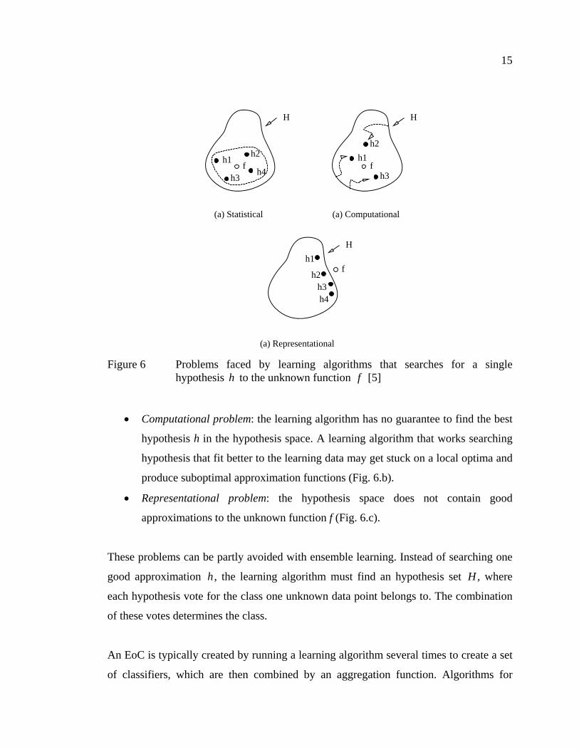
15
H
fh1
h2
h4h3
fh1
h2
h3
H
H
f
h4
h1
h2h3
(a) Statistical (a) Computational
(a) Representational Figure 6 Problems faced by learning algorithms that searches for a single
hypothesis h to the unknown function f [5]
• Computational problem: the learning algorithm has no guarantee to find the best
hypothesis h in the hypothesis space. A learning algorithm that works searching
hypothesis that fit better to the learning data may get stuck on a local optima and
produce suboptimal approximation functions (Fig. 6.b).
• Representational problem: the hypothesis space does not contain good
approximations to the unknown function f (Fig. 6.c).
These problems can be partly avoided with ensemble learning. Instead of searching one
good approximation h , the learning algorithm must find an hypothesis set H , where
each hypothesis vote for the class one unknown data point belongs to. The combination
of these votes determines the class.
An EoC is typically created by running a learning algorithm several times to create a set
of classifiers, which are then combined by an aggregation function. Algorithms for

16
creating EoCs will usually fall into one of two main categories. The first category
manipulates the training samples for each classifier in the ensemble. Two well-known
algorithms for this task are Bagging [41] and Boosting [42]. The second category
manipulates the feature set used to train classifiers, which can be performed through FSS
[12, 14, 43, 44], or through transformations on the feature set, as in the random subspace
approach [12, 14]. The key issue in this process is to generate a set of diverse and fairly
accurate classifiers for combination [6].
One trend in the PR literature is the optimization of ensemble of classifiers using genetic
optimization to select the most representative combination of hypothesis to increase
classification accuracy. Ruta and Gabrys used a GA in [11] to optimize the classifiers
aggregated on an EoC, whereas Oliveira et al. used a MOGA in [45].
1.1.6 Solution Over-Fit
Classifiers that are trained in several iterations, such as MLP classifiers, suffer from an
effect known as over-fit. Due to over-fit, the classifier memorizes the training data set,
instead of generalizing for unknown observations. To avoid the phenomena, a validation
stage is performed using unknown observations.
The same effect has been observed in the literature when optimizing classification
approaches using wrapped classifiers. Thus, solutions in the approximation set are
specialized to the optimization data set. Reunanen demonstrated solution over-fit to
compare sequential and floating FSS algorithms in [46]. In this context, solutions are
evolved based on the accuracy measured over an optimization data set.
Some solutions have been proposed in the literature to avoid the over-fit phenomena
during MOGA based classifier optimization. Loughrey and Cunningham discussed an
early stoping approach to remove over-fit from solutions optimized by GAs [47] and

17
simulated annealing [48]. Their iterative approach requires two stages. During the first
stage, solutions are optimized and validated to determine at which generation solutions
start to over-fit to the optimization data set, i.e., the generation where the algorithm has
to stop earlier. In order to avoid solution over-fit, the second stage uses this information
to optmize solutions until the previously calculated early stopping generation.
Llorà et al. used in [49] an approach that analyzed the optimized Pareto-front to
determine a rupture point. The rupture point divides the Pareto-front in two segments,
one over-fitted segment, and another segment where solutions provide higher accuracy
on unknown observations. The same approach was also used by Mansilla in [50].
Another known solution to this problem is related to a validation process. Instead of
selecting solutions using the traditional approach, i.e. based on the accuracy calculated
during the optimization process, a validation data set is used to select solutions in the
optimized Pareto-front. This approach was used in [51, 9, 52] and provided better results
than selecting solutions using the traditional approach.
1.2 State of the Art in Multi-Objective Genetic Algorithms
Real world optimization problems usually have many objectives to optimize. These
objectives are usually conflicting, i.e., improving one objective will decrease the quality
of conflicting objectives. The Min-Ex problem depicted in (1.1) [53] is a typical
unconstrained minimization problem with conflicting objectives, called a multi-objective
optimization problem (MOOP). Minimizing one function maximizes the other. This
forces the choice of a compromise between objectives before applying traditional
optimization methods. On traditional optimization methods, this compromise is
established using a weighted vector, as in (1.2), to create a single objective to direct the
optimization process.

18
( )( )
⎩⎨⎧
≤≤≤≤
+=
=
5011.0
:subject to
1Minimize
Minimize
2
1
1
22
11
xx
xxxf
xxf
(1.1)
f ev( )= w1 × f1 x( )+ w2 × f2 x( ) (1.2)
This approach is not optimal in the sense that the expert has to choose a specific trade-
off, whereas the set of possible trade-offs is unknown. For these optimization problems,
the optimal approach is that the algorithm finds the objective function trade-offs, and the
expert chooses the best solution based on a requirements analysis. Figure 7 depicts the
objective function space for the Min-Ex problem, where the bold line indicates the
optimal solutions with the best trade-offs. Such trade-offs are generated by a notion of
optimality, the Edgeworth-Pareto optimum or, simply, Pareto optimum. Solutions
belonging to the Pareto optimum set are referred as non-dominated solutions.
Multi-objective optimization algorithms work according to these principles, searching
for a solution set that presents the best possible optimization objectives trade-offs. One
specific class of algorithms is targeted in this thesis, the multi-objective genetic
algorithms (MOGA). These algorithms are based on the working principles of genetic
algorithms [1]. Schaffer introduced the Vector Evaluated Genetic Algorithm (VEGA) in
[54], which many consider to be the first MOGA. This algorithm used a modified GA
that selected solutions in turns using one objective function. It was Goldberg in [39] that
first hinted the possibility of using the concept of Pareto optimality to solve multi-
objective with GAs.
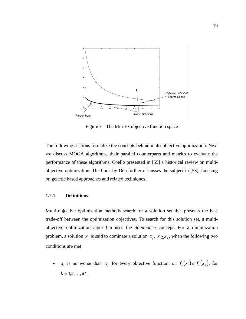
19
Figure 7 The Min-Ex objective function space
The following sections formalize the concepts behind multi-objective optimization. Next
we discuss MOGA algorithms, their parallel counterparts and metrics to evaluate the
performance of these algorithms. Coello presented in [55] a historical review on multi-
objective optimization. The book by Deb further discusses the subject in [53], focusing
on genetic based approaches and related techniques.
1.2.1 Definitions
Multi-objective optimization methods search for a solution set that presents the best
trade-off between the optimization objectives. To search for this solution set, a multi-
objective optimization algorithm uses the dominance concept. For a minimization
problem, a solution ix is said to dominate a solution jx , ji xx ≺ , when the following two
conditions are met:
• ix is no worse than jx for every objective function, or ( ) ( )jkik xfxf ≤ , for
Mk ,,2,1 …= .

20
• ix is strictly better than jx for at least one objective function, or
{ } ( ) ( )jkik xfxfMkk <∈∃ ,,,2,1, … .
These conditions indicate that ix has better objective function values than jx . If one of
the two conditions is broken, these solutions are uncomparable and they provide
different objective function trade-offs. In this situation, two solutions are said to non-
dominate each other. The following properties are valid for the dominance relation:
• Non-reflexive: a solution can not dominate itself.
• Non-symmetric: if ji xx ≺ , it is not possible by the dominance definition that
ij xx ≺ .
• Transitive: if ji xx ≺ and kj xx ≺ , it can be said that ki xx ≺ .
The bold line in Fig. 7 is composed of solutions that are non-dominated between each
other, but that dominate the remaining possible solutions. This set is called the non-
dominated set, or the Pareto front. For a specific set P of solutions, the non-dominated
set P′ is defined as { }pxpxPxPppP ≺/→≠∈∀∧∈=′ ,| . For the solutions in Fig. 8,
the non-dominated set is { }4,3,2,1=′P . The subset P′ of a set P is also known as the
approximation set. Thus, a multi-objective optimization method must optimize the
approximation set towards the problem’s true Pareto front.
Methods that solve MOOPs must accomplish two specific tasks:
• Find solutions close to the global non-dominated set.
• To evenly cover the global non-dominated set.

21
Figure 8 Min-Ex candidate solutions
These two tasks are conflicting, as they require two opposite aspects on search methods:
exploration and exploitation. Exploration searches the entire space for better solutions,
trying to get close to the non-dominated set, whereas exploitation search small areas to
cover the non-dominated set. The concept of dominance is useful to explore the search
space, as a non-dominated set will always be closer to the global non-dominated set. To
exploit the non-dominated set, metrics related to the distance between solutions are used.
Some well known metrics for this task are the sharing [56] (NSGA), the crowding
distance (NSGA-II) [57] and density estimation [58] (SPEA2).
1.2.2 Multi-Objective Genetic Algorithms
As the name implies, MOGAs are derived from genetic algorithms (GA) and follow the
same principles. Figure 9 depicts the flowchart of a GA. A population of candidate
solutions (individuals) evolve by means of genetic operations during a given number of
generations, aiming to increase individuals quality, measured by a fitness value.

22
Begin
Initialize Population
Cond?
gen = 0
Evaluation Assign Fitness
Stop
Reproduction
Crossover
Mutation
gen = gen + 1Yes
No
Figure 9 Classical GA flowchart
On each generation, individuals are evaluated and have their fitness assigned. Based on
this fitness, individuals are selected to reproduce, exchanging genetic information with a
crossover operator. To improve population diversity, individuals are often mutated
using a mutation operator. These two operators create the next generation of individuals,
which goes trough the same operations until the maximum number of generations is
reached. Spears studied in [59] the role of both operators with single objective GAs.
Recently, Ishibuchi and Narukawa compared in [60] the role of both operators in the
context of multi-objective optimization, associating crossover to exploitation and
mutation to exploration of the objective function space.
MOGAs follow a flowchart similar to Fig. 9, but changing the fitness to a non-
dominance based ranking, along with a metric to evenly space solutions in the Pareto-
front. Many works have reviewed and compared MOGAS. Deb discussed many
algorithms in [53], which was also done by Veldhuizen et al. in [61] and Zitzler et al. in
[62]. The Fast Elitist Non-Dominated Sorting Genetic Algorithm (NSGA-II) introduced

23
by Deb et al. in [63], which is used as the baseline MOGA for this thesis, is detailed in
Appendix 1.
1.2.3 Parallel MOGAs
To speedup the process and improve the solutions quality, studies have been made to use
MOGAs in parallel environments. Three primary models are considered, the master-
slave approach, the island model and the cellular model. These models employ concepts
similar to those of parallel GAs. Cantú-paz presented in [64] a complete study on the
issues of parallel GAs, where these three models are further detailed.
The master-slave model approach [65] is suitable to speed up the search on parallel
MOGAs. This is due to the fact that the algorithm does not change, it only assign the
evaluation of the objective functions to slave nodes, while the genetic operations are
made on a master node. Oliveira et al. in [30] used a master-slave parallel MOGA for
feature subset selection. The parallel cellular model is interesting for machines featuring
processor arrays. However, the high cost associated to these machines reduces the
interest on this specific research field, which focuses on specific problems that require
such processor organization.
The island model, also called distributed model, have seen an increase on research effort
after the Beowulf cluster computer boom. This type of cluster computer is based on
inexpensive workstations that are connected through a local network to exchange
information and complete a task. Cantú-Paz discussed in [64] the benefits of the island
models, posing questions on the differences between their sequential counterparts. He
also presented a survey of these algorithms in [66]. Hiroyasu et al. discuss in [67, 68]
two different approaches for MOGAs based on island models. Zhu and Leung proposed
in [69] an asynchronous MOGA with a self-adjustable objective space partitioning. A

24
similar concept is developed by Streichert et al. in [70], using clustering to partition ther
objective function space.
Our interest lies on the master-slave model, which provides speedup to the optimization
process, with no change to the optimization algorithm behavior.
1.2.4 Performance Metrics
Unlike GAs, MOGAs provide a solution set as the optimization process outcome. These
solutions are non-dominated, i.e., one solution can not be said to be better than the other.
This poses a problem when comparing the solution sets found by two different
algorithms, one can not directly compare these solutions. Any metric comparing two
different solution sets on MOOPs must address two aspects, the convergence towards
the global non-dominated set and its coverage.
Deb in [53] and Knowles in [71] reviewed techniques to evaluate different sets of non-
dominated solutions. Zitzler et al. recently compared current techniques in [72]. This
comparison established a mathematical framework developed for this task, dividing
performance metrics in two classes: unary and binary quality indicators. It was
concluded that unary quality indicators are limited, as they assign quality value to
approximation sets. Binary quality indicators are more powerful, as they assign a quality
value to the comparison of two approximation sets.
Examples of unary quality indicators are the spread [73], and the hypervolume indicator
[74]. Examples of binary quality indicators are the coverage [74] and the binary
hypervolume indicator, which compares the hypervolume covered by two approximation
sets based on the same reference point.

25
1.2.5 Discussion
This section discussed aspects associated to the research domains related to this thesis. It
has been observed that there is a lack of semi-automatic (eg. human centric)
methodologies to optimize and adapt classification systems, which encourages the
development of the classification system optimization approach covered in Chapter 2.
The optimized classification systems will be compared to a high performance baseline
representation, detailed in [51].
Over-fit in classification system optimization is an issue which is not often discussed.
Most papers in the literature that discuss this phenomena use small data sets, as in [49],
where the largest data set has 2048 observations. Thus, analysis with more significant
data sets is necessary to better understand this problem and propose an effective
solution.
Whereas two discussed papers use early stopping to halt the optimization process [47,
48], they did it as a mean to control over-fit. Instead, over-fit control should be
performed by a validation procedure, whereas a stopping criterion has to monitor the
optimized approximation set improvement to determine whether the algorithm must stop
or continue optimization.
The next chapter discusses an approach to optimize classification systems for isolated
handwritten symbols, based on both the pattern recognition and multi-objective
optimization techniques discussed in this chapter. The goal of such a system is to
optimize classification systems through multi-objective optimization based feature
extraction.

CHAPTER 2
CLASSIFICATION SYSTEMS OPTIMIZATION
In order to optimize classification systems, a multi-objective approach based on feature
extraction is proposed. This chapter details the approach, first presenting an overview in
Section 2.1 that introduces the approach components and roles. Sections 2.2 through 2.4
discusses the feature extraction, feature subset selection (FSS) and ensemble of
classifiers (EoC) optimization methodologies. Finally, a discussion in Section 2.6
concludes this chapter.
2.1 System Overview
Traditional image-based pattern recognition (PR) usually requires that pixel information
be first transformed into an abstract representation (a feature vector) suitable for
recognition with classifiers, a process called feature extraction [23, 75, 26, 22, 25]. A
relevant classification problem is intelligent character recognition (ICR), which is
aimed at recognizing handwritten symbols. One ICR application is the offline
recognition of isolated handwritten symbols on documents such as forms.
Methodologies for extracting features for this problem have been the subject of much
research [27, 24, 32].
A methodology that extracts features for PR must select the most appropriate
transformations and determine the spatial location of their application on the image. For
isolated handwritten symbols, the choice takes into account the domain context, which
type of symbols will be classified, and the domain knowledge, that is, what has been
previously done to solve similar problems. Such a process is usually performed by a
human expert (the experimenter) in a trial-and-error process specific to high-
performance ICR where accuracy improvements of 0.1% are relevant at the

27
classification stage. In high performance ICR, accuracy is around 99% and it is difficult
to further improve it, hence these small accuracy improvements are actually large
improvements on error rates on character strings. For a n characters string, the actual
expected accuracy is naccuracy . Given a 4 character string with a classifier that has
99.1% accuracy for individual characters, the expected accuracy for the 4 characters
string is %45.96%1.99 4 = . Another consideration is that changes in the domain context
manifest themselves not only when changing the PR problem, but the domain context
may change in the same classification problem, as illustrated in Fig. 1. To minimize the
burden on the human expert (the experimenter) in defining and adapting classifiers,
classifier optimization is modeled as an evolutionary MOOP, using the domain
knowledge introduced by its user as transformations to extract features and actual data
sets to represent the domain context.
Classification systems are modeled in two different two-level processes, as illustrated in
Fig. 10. In both processes, the first level uses the Intelligent Feature Extraction (IFE)
methodology to obtain the representation set IFERS (Fig. 10.a). The representations in
IFERS are used to train classifiers that are further processed on a second level. The
complexity of the best single classifier SI may be reduced through FSS (Fig. 10.b), or
all classifiers may be considered for aggregation on an EoC SE for improved accuracy
(Fig. 10.c).
Single classifiers and EoCs are both used for classification, but in different situations. A
single classifier is faster and suitable for classification systems running on hardware
with limited processing resources, such as embedded devices. An EoC demands more
processing power and is adequate for high-performance and robust classification
systems running on desktop or server computers. Thus, the approach can optimize the
classification stage in both situations according to its user needs.

28
Figure 10 Classification system optimization approach – representations obtained with IFE may be used to further improve accuracy with EoCs, or the complexity of a single classifier may be reduced through FSS
2.2 Intelligent Feature Extraction
Human experts are traditionally responsible for choosing the feature vector used in
classification systems. This vector is most often determined using domain knowledge
and domain context on a trial-and-error basis. This section details the Intelligent Feature
Extraction (IFE) methodology, which uses the domain knowledge and domain context in
an approach formulated as a MOOP to genetically evolve a candidate solution set. The
goal of IFE is to help the human expert define representations (feature vectors) in the
context of isolated handwritten symbols, using a wrapper approach with a fast training
classifier.
IFE models isolated handwritten symbols as features extracted from specific foci of
attention on images using zoning. This is a strategy known to provide better recognition
results than the extraction of features from the whole image [28, 27, 76]. Two operators
EoCOptimizationFSS
Coarse grain
FSSFine grain
IFE
SF
SC SE
RSIFESI
(a)
(b)
(c)

29
are used to generate representations with IFE: a zoning operator to define foci of
attention over images, and a feature extraction operator to apply transformations in
zones. The choice of transformations for the feature extraction operator constitutes the
domain knowledge introduced by the human expert. To obtain representations for
specific PR problems, such as digits or uppercase letters, the domain context is
introduced in the form of actual observations in the optimization data set used to
evaluate and compare solutions. Hence, IFE optimizes the zoning operator to the
selected feature extraction operator.
The IFE operators are combined to generate a representation such as illustrated in Fig.
11. The zoning operator defines the zoning strategy { }nzzZ ,,1 …= , where niz i ≤≤1,
is a zone in the image I and n the total number of zones. Pixels inside the zones in Z
are transformed by the feature extraction operator in the representation { }nffF ,,1 …= ,
where nif i ≤≤1, is the partial feature vector extracted from iz . At the end of the
optimization process, the resulting representation set { }pIFE FFRS ,,1 …= presents the
IFE user with a choice among various trade-offs with respect to the optimization
objectives, where p is the number of solutions optimized by the IFE.
Figure 11 IFE structure – domain knowledge is introduced by the feature extraction
operator, and the zoning operator is optimized based on the domain context (actual observations in the optimization data set)
The result set IFERS is used to train a discriminating classifier, creating the classifier set
{ }pKKK ,,1 …= , where iK is the classifier trained with representation iF . A
z2
z1
extractionoperator
Feature
I
z2
z1 F={f 1,f 2}
Zoning operator

30
traditional discriminating classifier used in classification systems is the multi-layer
perceptron (MLP) [2], which is targeted to train K . The first hypothesis is to select, in
K , the most accurate classifier KSISI ∈, for a single classifier system. In this
hypothesis, SI can be further optimized to reduce its feature set cardinality through
feature subset selection, which is discussed in Section 2.3. The second hypothesis is to
use K to optimize an EoC for higher accuracy, an approach discussed in Section 2.4.
The remainder of this section discusses the IFE operators chosen for experimentation
with isolated handwritten digits and the candidate solution evaluation.
2.2.1 Zoning Operators
The zoning operator is the key element to optimize representations with the IFE. The
domain knowledge introduced by the IFE user plays an important role, however, the
crucial task to determine the actual locus of extraction is performed by the zoning
operator. This section discusses two different zoning operators for the IFE. These
operators performance will be compared later in Chapter 6.
2.2.1.1 Divider Zoning Operator
A baseline representation is considered for reengineering to compare IFE to the
traditional human expert approach. This representation is known for its high degree of
accuracy on isolated handwritten digits with a MLP classifier [51]. Its zoning strategy,
detailed in Fig. 12.b, is defined as a set of three image dividers, producing 6 zones. The
divider zoning operator expands the baseline zoning concept into a set of 5 horizontal
and 5 vertical dividers that can be either active or inactive. Fig. 12.a details the operator
template.

31
Figure 12 Divider zoning operator – each divider is associated with a bit on a binary
string (10 bits), indicating whether or not the divider is active; the baseline representation in (b) is obtained by setting only d2, d6 and d8 as active
The divider zoning operator is genetically represented by a 10-bit binary string. Each bit
is associated to a divider’s state (1 for active, 0 for inactive), producing zoning strategies
with 1 to 36 zones. Figure 13 illustrates an example, relating both the binary coding
string and its associated zoning strategy with 4 zones.
Figure 13 Divider zoning operator example
Genetic operations are performed on the binary string as usual, changing the bits to
evolve the current population. Figure 14 illustrates the single point crossover operator on
d0 d1 d2 d3 d4
d5
d6
d7
d8
d9
0 1 0 0
0101
0
0
(b)(a)
d2 d3 d4 d5 d6 d7 d8 d9d1d0
0 1 0 00
0
0
0
1
0
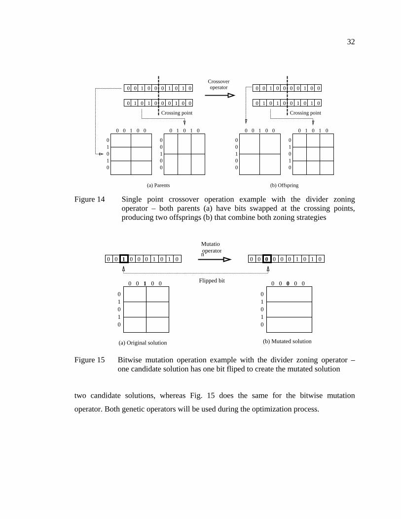
32
Crossoveroperator
0000
0
0
0
000
0
0
1
1
1
1 1
10
0
0 0 0 00 001 1 1
0 0 0 0 0 0 11 01
(a) Parents (b) Offspring
Crossing point
0000
00
00
0100
01010
1
1
1
0 0 0 01 00
0 0 0 01 1
0 0 1
0 0 11
Crossing point
Figure 14 Single point crossover operation example with the divider zoning
operator – both parents (a) have bits swapped at the crossing points, producing two offsprings (b) that combine both zoning strategies
Figure 15 Bitwise mutation operation example with the divider zoning operator – one candidate solution has one bit fliped to create the mutated solution
two candidate solutions, whereas Fig. 15 does the same for the bitwise mutation
operator. Both genetic operators will be used during the optimization process.
Mutatio
n operator
00 0 0 0
0
0
1
1
1
(a) Original solution
0 0 0 0
0
0
0
1
1
0
(b) Mutated solution
0 0 0 0 0 11 01 0 0 0 1 0 0 0 1 0 0 0
Flipped bit

33
2.2.1.2 Hierarchical Zoning Operator
This zoning operator defines the zoning strategy based on a set of zoning patterns,
depicted in Fig. 16 and associated to an integer number. Each pattern has labeled
partitions that can be recursively partitioned with other patterns from the set. This
strategy is described as a tree, where a root pattern is further partitioned by leaf patterns
associated to its original partitions. Figure 17 illustrates an example of this strategy with
one recursion level. Recursion is limited to one level to experiment with the IFE, hence
the number of zones that can be defined with this operator range between 1 to 16.
The operator is genetically represented by a 15 bits binary string. Each pattern is
represented as a 3 bits binary substring, mapping to one of the eight zoning patterns
through traditional binary to decimal conversion, where a is encoded as 0 and h is
encoded as 7 (these values are indicated for each zoning pattern in Fig. 16). The
complete coding requires a root pattern and 4 leaf patterns, therefore the genetic
representation for this operator requires a 15 bits binary string, as demonstrated in Fig.
17.c.
A B
D C
(a) 000
A
D C
(b) 001
BD
A
(c) 010
A
C
B
(d) 011
AB
C
(e) 100
BA
(f) 101
C
A
(g) 110
A
(h) 111
Figure 16 Hierarchical zoning pattern set and associated 3 bits binary strings

34
(a)
0 0 0 0 0 00 0 0 0 0
C DBRoot A
1 1 1 1
(c)
(b)
A
CD
AC
D
Figure 17 Zoning strategy encoded as egba# (a), its associated zoning tree (b) and binary string (c)
The example in Fig. 17 has one inactive pattern, as partition B does not exist in the root
pattern selected. In this case, the encoded value is ignored during feature extraction,
however, it is still considered during genetic operations as it can become active at some
moment. This operator can produce 5768 different zoning configurations, while keeping
a small feature set dimensionality, with a maximum of 16 zones against a maximum of
36 zones provided by the dividers zoning operator.
As with the divider zoning operator, genetic operations are performed as usual over the
binary string. Figure 18 illustrates the single point crossover operator on two candidate
solutions, whereas Fig. 19 does the same for the bitwise mutation operator. Again, both
genetic operators will be used during the optimization process. In both figures, the less
significant bit is the leftmost bit in the string.

35
0 0 0 0 0 00
1 1 1 111 1Crossoveroperator0 0
0 1 10 11 1
0 0 0 0 0 0 0 0 00
1 1 1 11
0 0 0
0 1 1
Crossing point
(a) Parents
0 0
0 1 10 11 1
0 0 00 0 0
0
Crossing point
(a) Offspring
Figure 18 Single point crossover operation example with the hierarchical zoning operator – both parents (a) have bits swapped at the crossing points, producing two offsprings (b) that combine both zoning strategies
00 0 0 0 0 0 0 0 000 0 0 operatorMutation
0 0 00 00 0 00 00 0 00 10
(a) Original solution. (b) Mutated solution.
Figure 19 Bitwise mutation operation example with the hierarchical zoning operator – one candidate solution has one bit fliped to create the mutated solution
2.2.2 Feature Extraction Operator
Oliveira et al. used and detailed in [51] a mixture of concavities, contour directions and
black pixel surface transformations, extracting 22 features per zone (13 for concavities,
8 for contour directions and 1 for surface). To allow a direct comparison between IFE
and the baseline representation, the same feature extraction operators (transformations)
are used to assess IFE with isolated handwritten digits.

36
Heutte et al. discussed in [26] the concept of concavities transformation. For every white
pixel in the image in Fig. 20.a, we search in 4-Freeman directions (Fig. 20.b) for black
pixels and determine the directions we reach black pixels and the directions we do not. If
we find black pixels in all directions, we search in four auxiliary directions (Fig. 20.c) to
confirm that the white pixel is inside a closed contour or not. Pixels that reach only one
black pixel are ignored as they are not inside a concavity. For each zone the
transformation produces the 13 positions feature vector in Fig. 20.d, where the first line
labels the number of directions that black pixels can be reached, the second line labels
the directions we find white pixels (for pixels on an open contour) and the last indicates
the pixel count associated to that feature. Two examples in Fig. 20.a illustrates the
process, pixel 1x reaches four black pixels but fails to find black pixels in direction 1S ,
and pixel 2x reaches three black pixels and misses direction 1.
Figure 20 Concavities transformation, as used in [51]
The contour direction transformation is performed with a histogram of contour
directions. For each zone in the image, contour line segments are labeled clockwise and
counted regarding the 8-Freeman directions in Fig. 21.b, producing the 8 features vector
S1 S2
S3S4
(c)
0
13
2
(b)
2 2 2 3
0,1 1,2 2,3 3,0 0 1 2 3
3 3 3 4 4 4 4 4
1
2
--
1
10 110 1 2 3 4 5 6 7 8 9 12
(d)
S1 S2 S3 S4 Black Pixels:
White pixels:
Feature vector:
Label:
x1
x2
(a)

37
in Fig. 21.c. The example in Fig. 21 details the contour count for the highlighted zone in
the image. The first line is the direction count in this zone, whereas the second line is the
associated Freeman direction.
Finally, the surface transformation simply indicates the number of black pixels in each
zone. Thus, the surface transformation produces one feature. For proper comparison
between different sized images, all extracted features (concavities, contour and surface)
are normalized between 0 and 1 regarding all zones. For each individual feature
extracted we calculate its total value on all zones and normalize values in zones in the
[ ]1,0 interval.
2.2.3 Candidate Solution Evaluation
Candidate solutions are evaluated with respect to two objective functions, quality and
dimensionality. Representation quality is related to classification accuracy, whereas
representation dimensionality (feature number) is related to the generalization power
associated with the representation. If the dimensionality is too high, the classifier tends
to memorize the training set, an effect called the curse of dimensionality. Classification
(b)
01
2
35
6
7
4
(a)
0 1 2 3 4 5 6 7
(c)
0 3 2 1 1 3 01Feature vector:
Label:
Figure 21 Contour direction transformation, as used in [51]

38
processing time is also related to representation dimensionality: the more features
associated with the representation, the longer it takes to classify unknown observations.
Dimensionality is measured as the representation zone number, given that, for IFE, the
same feature vector is extracted from all zones. To evaluate representation quality, two
strategies are discussed by John et al. in [77], the filter and wrapper approaches. The
filter approach evaluates the representation based on measures over the representation
itself, while the wrapper approach evaluates representation performance with actual
classification. Chen and Liu indicate in [78] that a wrapper approach is better when the
objective is classifier performance. Hence, this approach is the best choice for IFE, as
the objectives are to minimize both dimensionality and the classification error rate on the
optimization data set.
Robust and efficient classification systems require fast and discriminating classifiers.
Two common classifiers in these systems are the MLP and support vector machine
(SVM) [3, 4] classifiers. Both the MLP and SVM classifiers are fast and accurate in
classification tasks. However, their training procedure is time-consuming and requires
optimization of the configuration parameters. The wrapped classifier needs to be
computationally efficient and reasonably accurate to prototype IFE solutions. Kimura et
al. discussed in [79] the projection distance (PD) classifier. Based on hyperplanes to
model classes, the PD classifier fairly quickly trains and classifies observations,
modeling each class iω , a set of learning samples, as a hyperplane. An unknown
observation x is projected on the hyperplane with (2.1). The projection ( )xPi is used to
calculate the Euclidean distance to the actual observation x . The projection closest to
the actual observation determines the class that the observation x belongs to.
( ) ( ) iiii xxP μμ +ΨΨ−= (2.1)

39
On (2.1) we have that iΨ are the first k eigenvectors of the covariance matrix iΣ of iω ,
ordered from the highest to the lowest value of eigenvalues. iμ is the mean vector of the
learning samples iω . Based on these working principles, the PD classifier tends to relate
the problem classes to compact and well separated clusters that are used for the
classification stage, providing higher accuracy than nearest neighbor (NN) classifiers.
Also, the PD classifier requires less processing time to train and evaluate IFE solutions
than NN or MLP classifiers. Therefore, the PD classifier has been chosen for the
wrapper approach used to evaluate IFE representations through the optimization process.
Training a PD classifier requires two data sets, a training and a validation data set. The
training data-set is used to create the hyperplane models, whereas the validation data set
is used to optimize the k value. The PD classifier accuracy on the validation data-set is
tested for all k values and the highest accuracy is selected to evaluate unknown
observations. The process to select k is illustrated in Fig. 22.
0 10 20 30 40 50 60 70 80 90 1002
4
6
8
10
12
14
16
18
3.52
k
Erro
r rat
e
Figure 22 PD clasisfier k values during the training procedure and the associted
error rates : the lowest error rate on the validation data set is obtained with 30=k , yielding a 3.52% error rate

40
2.3 Feature Subset Selection
Feature subset selection (FSS) [77, 40, 80, 43] aims to optimize the classification
process, thereby eliminating irrelevant features from the original representation in order
to create a smaller, yet accurate, representation. FSS is primarily used to reduce the
computational cost associated with extracting and classifying unknown observations,
which is important for embedded devices with limited processing resources. Due to the
curse of dimensionality, which favors smaller representations, FSS may also improve
classification accuracy by eliminating irrelevant features. The FSS problem is defined as
finding a good feature subset regarding some objective function [77]. For the FSS
methodology in this section, the objective functions are to minimize classification error
and representation cardinality.
Kudo and Sklansky compared FSS techniques in [35], concluding that a GA performs
better when the original representation size is large (more than 50 features). Oliveira et
al. applied a GA-based FSS in [81] using a weighted vector with isolated handwritten
digits, postulating that a MOGA could further enhance the results obtained. Their
postulate was later confirmed in [10], where the MOGA outperformed the GA on the
same problem. The superiority of MOGA in FSS is also confirmed by Emmanouilidis et
al. [9] using sonar and ionosphere data.
FSS in this chapter is applied on the representation SI obtained with the IFE
methodology. The FSS problem is modeled as a MOOP with two different levels (Fig.
10.b). The feature vector extracted for each zone in IFE is a combination of features
produced by different transformations (concavities, contour directions and black pixel
surface). Thus, a two-level FSS operation is proposed, where a coarse grain FSS
optimization removes transformations applied on zones in SI (the single classifier
optimizaed by the IFE), producing the representation SC . Next, a fine grain FSS
optimization removes individual features in SC , producing the representation SF . The

41
coarse grain FSS removes large blocks of features, leaving a reduced feature set in SC
for further processing with the fine grain FSS. The fine grain FSS is similar to traditional
FSS approaches and can be applied directly to representation SI for comparison
purposes.
Li and Suen discussed in [32] the impact of missing parts in handwritten recognition,
zones with no features extracted. According to the concept of missing parts, the pixel
information in some zones of image I are ignored, as illustrated in Fig. 23. It was
observed in their experiments that removing entire zones from the feature extraction
process improved classification accuracy. This process relates to the FSS process, and
therefore it is desirable to emphasize missing parts in solution encoding and its
evaluation process.
Missing part
I
Figure 23 Missing parts example – marked zones are inactive and no features are
extracted for classification (the example has 7 active zones)
Candidate solutions in both FSS levels are represented with binary vectors (Fig. 24).
Each bit in the coarse grain FSS binary vector cg is associated with the state of a
transformation applied to a zone (1 if the transformation is applied and 0 otherwise). As
for the fine grain FSS, each bit in the binary vector fg is associated with the state of an
individual feature (1 if the feature is active and 0 otherwise). Missing parts in both FSS
levels are obtained when all bits related to a zone are set to 0, eliminating all features

42
Figure 24 Feature subset selection procedure on an one zone solution SI (22 features) : the contour directions transformation has been removed from the feature vector SI by the coarse grain FSS, producing the feature vector SC (a); individual features in SC are removed with the fine grain FSS to produce the final representation SF (b)
extracted. The process is illustrated in Fig. 24 for a theoretical one-zone representation
using the concavities (c), contour directions (d) and black pixel surface (s) transforma-
tions.
Two objective functions guide the optimization process in both FSS levels,
representation cardinality and representation quality. To explicitly emphasize missing
parts, representation cardinality is defined in both FSS levels as the active zone number,
i.e. zones having at least one feature extracted. Representation quality is measured
through a wrapped classifier. The MLP classifier is targeted with the IFE experiments,
and thus the same classifier is targeted for FSS. Because of the time required to train
MLP classifiers, it is not feasible to train actual MLP classifiers to evaluate candidate
solutions. Instead, sensitivity analysis [82] is used to estimate the relevance of MLP
0.03 0.01 0.04 0.040.03 0.01 0.080.09
d1 d2 d3 d5 d4 d6 d7d0
c sd
101cg
0 1 1 1 1
c8 c9 c10 c11 c12
1 0 1 0 0
c3 c5 c6 c7c1 c2 c0 c4 fg
0.07 0.0 0.0 0.01 0.0
c8 c9 c10 c11 c12
0.03 0.04 0.01 0.06 0.040.01 0.01
c3 c5 c6 c7c1 c2 0.02
c0 c4 SC
s
0 0 1 1
0.0 0.0 0.0 0.2
c9 c10 c11 c12 sc2 c3 c5 0.01 0.03 0.02 SF
0.07 0.0 0.0 0.01 0.0
c8 c9 c10 c11 c12
0.03 0.04 0.01 0.06 0.040.01 0.01
c3 c5 c6 c7c1 c2 0.02SI
c0 c4
0.07 0.0 0.0 0.01 0.0
c8 c9 c10 c11 c12
0.03 0.04 0.01 0.06 0.040.01 0.01
c3 c5 c6 c7c1 c2 0.02
c0 c4 SC
0.2
s
0.2
s
0.2
s
0.01
(a) Coarse grain feature subset selection operation
(b) Fine grain feature subset selection operation

43
inputs (features) and classification performance. Given a data set with N observations,
the neural network sensitivity iS to variable i (a feature) is defined in (2.2), where ijS is
the calculated sensitivity to observation jx in (2.3) and x is calculated as in (2.4).
∑=
=n
jiji S
NS
1
1 (2.2)
( ) ( )ijiij xSExSES −= (2.3)
∑=
=n
jijx
Nx
1
1 (2.4)
iS measures the impact on the trained square error ( SE ) of replacing the MLP input
associated to feature i by the calculated average ix for all N training observations.
Moody and Utans demonstrated in [82] that MLP inputs are irrelevant if they can be
replaced by their average in the training data set. Each feature corresponds to an MLP
input, thus the MLP classifier is trained once with SI , and features removed in both FSS
optimization levels are replaced by their training data set average during the
optimization process. At the end of the optimization process, candidate solutions are
trained with MLP classifiers to obtain the actual performance of reduced representations
for selection.
Thus, the objective functions minimized for both FSS levels are the representation error
rate and the number of active zones. The result of each FSS optimization level is a
solution set CGRS for the coarse grain FSS, and FGRS for the fine grain FSS. In both
levels, the most accurate representations CGRSSCSC ∈, and FGRSSFSF ∈, are
selected (Fig. 24.b) for classification ( SF ) or to continue the FSS procedure ( SC ).

44
2.4 EoC Optimization
A recent trend in machine learning has been to combine several learners to improve their
overall performance [5]. Thus, classifiers can be combined to improve the classification
stage in PR systems. An EoC is typically created by running a learning algorithm several
times to create a set of classifiers, which are then combined by an aggregation function.
Algorithms for creating EoCs will usually fall into one of two main categories. The first
category manipulates the training samples for each classifier in the ensemble. Two well-
known algorithms for this task are Bagging [41] and Boosting [42]. The second category
manipulates the feature set used to train classifiers, which can be performed through FSS
[12, 14, 10, 44], or through transformations on the feature set, as in the random subspace
approach [13, 15]. The key issue in this process is to generate a set of diverse and fairly
accurate classifiers for combination [6].
Ruta and Gabrys used a GA in [11] to optimize the classifiers aggregated on an EoC.
This section details a two-level methodology to create an EoC as a MOOP. The first
level creates a classifier set with IFE, and the second level optimizes the classifiers
aggregated using a MOGA. As each classifier is trained with a different representation
produced by IFE, this approach belongs to the second class of EoC algorithms. The
proposed EoC methodology selects which classifiers to aggregate from the set
{ }pKKK ,,1 …= , where iK is the classifier trained with the representation iF in the
IFE result set { }pIFE FFRS ,,1 …= . This hypothesis assumes that IFERS generates a set
K of p diverse and fairly accurate classifiers. To realize this task as a MOOP, the
classifiers in K are associated with a binary string E of p bits, which is optimized to
select the best combination of classifiers using a MOGA. The classifier iK is associated
to the thi binary value in E , which indicates whether or not the classifier is active in the
EoC.

45
The optimization process is guided by two objectives, EoC cardinality and EoC quality.
Computational effort during classification is related to EoC cardinality: the smaller the
EoC, the less computational effort is required to classify observations. Ruta and Gabrys
postulated in [11] that combined classifier performance (the wrapper approach) is a
reliable and meaningful criterion with which to compare EoCs, and works well with
most search algorithms. Thus, EoC quality in this methodology is evaluated with a
wrapper approach, using the aggregated classifier output to evaluate accuracy. The goal
is to minimize both EoC cardinality and the associated error rate on the optimization
data set.
Evaluating the EoC error rate requires actual classifier aggregation, which depends on
the classifier employed. The normalized continuous values of MLP classifier output are
aggregated by their output average [6]. To speed up the process, the MLP outputs are
calculated once only, and their actual aggregation is calculated during runtime. PD
classifiers are aggregated by majority voting. As with MLP classifiers, PD votes are
calculated once only, and the votes are counted during runtime.
2.5 Optimization Algorithm Requirements
To better understand the optimization problem and verify the impact of over-fit, a study
was conducted with the IFE using the divider zoning operators and the digits data sets in
Table I. Samples in each class are equally distributed in each data set for a more relevant
analysis. The wrapped PD classifier is trained with the learn data set and the validation
data set to configure classifier parameters during learning. The optimization data set is
used with the wrapped classifier to evaluate the objective function associated to
representation accuracy (actually, the error rate). In order to verify the generalization
power of solutions optimized by the IFE, the unknown data set is used to compare the
error rates on observations unknown to the optimized solutions.

46
Figure 25.a partially details the error rates of solutions in the objective function space,
where each point relates to a trained PD classifier. Solutions A and C are dominated by
solution B in the optimization data set objective space (Fig. 25.a). In this context,
solution B belong to the Pareto-optimal set. Solutions A and B have the same
cardinality, but the later has lower error rate, and solution B outperforms solution C in
both feature set cardinality and accuracy. Changing the context to the unknown data set
to evaluate the error rate in Fig. 25.b, solution B is dominated by solution A , and
solution C becomes non-dominated. Both solutions A and C belong to the Pareto-
optimal set in the unknown data set context. Thus, solution B is over-fitted to the
optimization data set and does not perform as well on observations unknown to the
optimization process.
Table I
Handwritten digits databases extracted from NIST SD19
Database Size Origin Sample range learn 50000 hsf_0123 1 to 50000
validation 15000 hsf_0123 150001 to 165000 optimization 15000 hsf_0123 165001 to 180000
unknown 15000 hsf_0123 180001 to 195000
Because of the non matching objective function spaces, it is clear that traditional Pareto-
based approaches will not always emphasize and explore solutions with good
generalization power on unknown observations. This preliminary analysis led to two
requirements to be satisfied by an MOGA algorithm to proper optimize classification
systems:
1. Allow the optimization of dominated areas in the decision-frontier to find
solutions similar to C in Fig. 25.

47
(a) optimization data set
(b) unknown data set
Figure 25 Objective function space associated to different data sets – the optimization data set is used to evaluate candidate solutions and guide the optimization process, whereas the unknown data set is used to verify the solutions generalization power
2. Archive different levels of accuracy regarding solutions cardinality to keep
solutions as A in Fig. 25 for validation.
Both requirements are satisfied by the Multi-Objective Memetic Algorithm (MOMA),
which is detailed in Chapter 3, the first approach used to solve the over-fit issued
verified in this analysis. Later it was observed that MOMA was limited by its
configuration parameters and a more robust approach was needed, leading to a complete
strategy to control over-fit, which is discussed in Chapter 4.
2.6 Discussion
This chapter detailed an approach to optimize classification systems, based on three
methodologies that optimize classification systems for two contexts as MOOPs. The

48
approach can optimize solutions for both single and multiple classifier systems. Most
importantly, the approach uses the domain context and the domain knowledge
introduced by an human expert to automatically optimize solutions, thus reducing the
human intervention in creating and adapting classification systems. This chapter also
introduced the over-fit issue, which will be addressed in the following chapters.
The next chapter proposes and discusses a multi-objective optimization algorithm
adapted to the issues discussed in Section 2.5. The Multi-Objective Optimization
Memetic Algorithm (MOMA) provides mechanisms to overcome the limitations
associated to traditional Pareto-based approaches when optimizing classification
systems.

CHAPTER 3
MULTI-OBJECTIVE OPTIMIZATION MEMETIC ALGORITHM
This chapter details the Multi-objective Optimization Memetic Algorithm (MOMA),
discussing the motivations to design the algorithm, its concepts and the pseudo-code of
each stage of the algorithm. The algorithm is adapted to the IFE and similar
methodologies. This algorithm is then tested with the IFE to optimize representations for
isolated handwritten digits with several configurations parameters and the results are
discused.
MOMA combines a traditional MOGA with a local search algorithm to create a more
powerful search mechanism for the IFE, and belong to a class of algorithms known as
memetic algorithms (MA), which has been the subject of recent research [83, 84, 85,
86]. Jaszkiewicz demonstrates in [87] that hybrid optimization methods outperform
methods based solely on genetic operations, hence the interest in developing MOMA, a
two-objective optimization algorithm that combine GA with a local search (LS)
algorithm.
3.1 Algorithm Concepts
Two requirements were defined in Chapter 2 to optimize classifications systems. One is
to optimize for each cardinality value the best solution for selection. This set of solutions
is called thereafter the decision front. Another requirement is to archive for each
cardinality value a set of solutions for the selection stage. Thus, an algorithm adapted to
this problem must optimize the decision front and archive a set of solutions ranked by
decision frontier levels.

50
To perform this task, objective functions are divided in two categories, objective
function one ( 1o ) in the integer domain, that defines the slots in the auxiliary archive S ,
and objective function two ( 2o ), which is optimized for each 1o value. To archive
different levels of performance, each slot lS is a set of lSmax solutions, associated to a
possible 1o value. For the approach to optimize classification systems, 1o is the feature
set/EoC cardinality and 2o is the representation error rate.
The archive is defined as { }JSSS ,,1 …= , where J is the maximum number of slots.
For solution ix , ( )ixo1 and ( )ixo2 are the solution’s values of 1o and 2o .
( ) lbbl SxxSB ∈= , , such as that ( ) ( )( ) ljjb Sxxoxo ∈∀= ,min 22 , indicates the solution bx
in lS with the best 2o value, whereas ( ) lwwl SxxSW ∈= , , such as that
( ) ( )( ) lwkw Sxxoxo ∈∀= ,max 22 , indicates the opposite.
The decision frontier set SP optimized by the MOMA algorithm is defined as
( )}{1
lJ
lS SBP
== ∪ . We indicate that solution ix is admissible into slot lS as
( ) lxoSx ili =≡Θ 1 , then ( ) { }ll ScCccCSA Θ∈∀= ,|, denotes the subset of solutions in
C that are admissible in lS .
To optimize the decision frontier as indicated in Fig. 25, solutions are ranked for genetic
selection by a frontier ranking approach. In the population P , the solution set belonging
to the first rank is defined by ( )( )},{1
1 PSABR lJ
l== ∪ . The solution set belonging to the
second rank 2R is obtained as the first rank of 1\ RP , and so on.
The decision frontier concept and the archive S are key elements for proper
optimization of classification systems using validation at the last generation. Combined,

51
they provide means to select solutions after optimization based on their generalization
power on unknown observations. Selecting solutions by the decision frontier allows the
optimization of solutions usually discarded by traditional Pareto based approaches. This
need is justified to avoid optimization bias as indicated in Fig. 25, where solution C is
dominated in the IFE model optimization objective space using the optimization data set,
but has better generalization power on unknown observations. The same principle
justifies the need to store different levels of performance in the slot, solution A in Fig.
25 has better generalization power on unknown observations, but would be discarded
from the archive on traditional approaches.
3.2 Algorithm Discussion
The MOMA algorithm is depicted in Fig. 26. It evolves a population P of size m , and
archives good solutions found in the slots S , which are updated at the end of each
generation. The population P is initialized in two steps. The first creates candidate
solutions with a Bernoulli distribution, while the second generates individuals to
initialize the slots. For each slot, we choose one random solution that is admissible in the
slot and insert it in the population.
During genetic optimization, individuals in the current generation tP are subjected to
frontier ranking. Next a mating pool M is created by tournament selection as indicated
in Algorithm 1, followed by traditional crossover and mutation to create the offspring
population 1+tP . In case of a draw in the tournament selection and both individuals are
uncomparable (belong to the same frontier rank), one of the solutions is chosen
randomly.
Parks discussed in [88] the effects of genetic overtake due to multiple copies of the same
individuals, which degrade the performance of evolutionary algorithms. To avoid

52
Figure 26 MOMA algorithm
Algorithm 1: Tournament selection operator for MOMA Data: Current population tP Result : Mating pool M repeat Select solutions tPqp ∈, , such as that both p and q have not yet participated two times in tournaments; if qp then { }pMM ∪= ; else if qp then { }qMM ∪= ; else Randomly selects individual r from { }qp, ; { }rMM ∪= ; end end until mM = ;
on solutions in Pt+1
Applies the RRT algorithm
Start
End
Update Slots
pool M from PCreates mating
individuals in Pt+1
Gen
etic
opt
imiz
atio
n Lo
cal s
earc
h
t=t+1
Yes No
Modify redundant
of crossover and mutation Creates Pt+1 by means
Stop?
Initialize

53
genetic overtake, redundant individuals are mutated until the population has no
redundant individuals as in [11]. To avoid checking every individual against the entire
population and to improve algorithm efficiency, individuals are tested for redundancy as
they are inserted into 1+tP . The algorithm to achieve this taks is described in Algorithm
2. This algorithm tests if 1+∉ tPp , and if true, p is inserted into 1+tP . Otherwise, if 1+∈ tPp , the algorithm mutates p until 1+∉ tPp before insertion. To verify that 1+∈ tPp it is usually enough to verify the binary string equality between p and all
candidate solutions in 1+tP . It should be noted that the hierarchical zoning operator may
produce the same zoning strategy with two different binary strings, thus the test to verify
if 1+∈ tPp should consider for comparison the actual representation associated to
solutions when optimizing the IFE with the hierarchical zoning operator.
After genetic optimization, solutions are further improved by a LS algorithm. The
algorithm chosen is the Record-to-Record Travel (RRT) algorithm [89], an annealing
based heuristic. The RRT algorithm improves solutions by searching in its neighborhood
for n potential solutions during NI iterations, allowing a decrease in the current
performance of %a to avoid local optimal solutions as indicated in Algorithm 3.
Algorithm 2: Algorithm to insert an individual p into population 1+tP Data: Population 1+tP and solution p Result : Modified population 1+tP if 1+∉ tPp then { }pPP tt ∪= ++ 11 else while 1+∈ tPp do mutate p ; end { }pPP tt ∪= ++ 11 ; end

54
Neighbors to solution ix must have the same feature set cardinality and similar
structure, which is achieved in the IFE model by modifying the zoning operator
encoding. For the divider zoning operator, dividers are distributed in two groups, and
{ }987652 ,,,, dddddg = . To generate a neighbor we select a group to activate one divider
and deactivate another. The solution in Fig. 27.a has solutions in Figs. 27.b and 27.c as
two possible neighbors. To create a neighbor to the hierarchical zoning operator, the
algorithm changes one zoning pattern while keeping the same feature set cardinality.
This process is illustrated in Fig. 28, where solution in Fig. 28.a has two neighbors in
Figs. 28.b and 28.c. For EoC and fine grain FSS methodologies, two different binary
values are swapped in the bit string. The coarse grain FSS follows a similar approach,
however, the binary values swapped must belong to the same feature extraction operator.
Algorithm 3: Record to record travel (RRT) algorithm used by MOMA to further optimize solutions Data: Population P Result : Modified population P forall Pxi ∈ do 0=iterations ; ixp = ; ( )poRECORD 2= ; repeat Choose a random set of solutions J , nJ = , neighbor to p ; Select the best solution Jp ∈′ ; if ( ) ( )aRECORDpo +×<′ 12 then pp ′= ; if ( ) RECORDpo <′2 then ( )poRECORD ′= 2 ; pxi = ; end end 1+= iterationsiterations ; until NIiterations = ; end

55
(a) (b)
(c)
Figure 27 Divider zoning operator example – zoning strategy (a) and two neighbors (b and c)
(a) aeefe (b) acefe
(c) aeege
Figure 28 Hierarchical zoning operator – zoning strategy (a) and two neighbors (b and c), with associated zoning patterns (the bold letters indicate the zoning pattern replaced to create the neighbor solution)
After the LS, the archive S is updated, storing good solutions from 1+tP in the slots as
in Algorithm 4. Recall that lSmax is the maximum number of solutions a slot can hold.
At this point, the stopping criterion is verified, deciding if the algorithm should continue
to the next iteration or stop the optimization process.
3.3 MOMA Validation Tests with the IFE
A model was created to verify MOMA, based on the IFE using the dividers zoning
operator. The entire objective function space was calculated (all 1024 possible
solutions), evaluating the representations discriminative power on a wrapper approach
using actual PD classifier performance. The PD classifier details and training procedure
are presented in Section 2.2.3. Classifier training and error rate evaluations were made

56
with the digits databases in Table II. The disjoint databases are extracted from the
NIST-SD19 database, using the digits data sets hsf_0123 and hsf_7. Both the feature set
cardinality and the error rate are minimized in these experiments.
PD classifiers were trained using the learn data set as the learning examples, and the
validation data set to configure classifier parameters during learning. Error rate during
the IFE optimization is calculated with the trained classifier on the optimization data set.
To verify the generalization power of solutions optimized by the IFE, the selection and
test databases are used to compare the error rates on unknown observations.
Table II
Handwritten digits databases used to validate MOMA
Database Size Origin Sample range learn 50000 hsf_0123 1 to 50000
validation 15000 hsf_0123 150001 to 165000 optimization 15000 hsf_0123 165001 to 180000
selection 15000 hsf_0123 180001 to 195000 test 60089 hsf_7 1 to 60089
Algorithm 4: MOMA update slot algorithm Data: Population P and the auxiliary archive S Result : Modified auxiliary archive S forall Pxi ∈ do ( )ixol 1= ; if ( ) ( )( ) lili SxSWoxo ∉∧< 22 then { }ill xSS ∪= ; if lS
lS max> then
( ){ }lll SWSS \= ; end end end

57
3.3.1 Algorithmic Parameters
MOMA has a parameter set to configure, both for the genetic optimization and the local
search stages. The list bellow indicates parameters that will be verified:
• m : population size
• cp : crossover probability
• mp : mutation probability
• n : size of the neighbourhood S for the RRT algorithm
• a : parameter to configure the deviation for the RRT algorithm
• NI : the maximum number of iterations for the RRT algorithm
The MOMA algorithm has another parameter that does not change directly its
performance in terms of exploratory power, lSmax , the maximum number of individuals
inside each slot. This parameter does not need optimization and is based on user
preferences, related to the optimization problem. For instance, lSmax may be
determined based on the number of frontier levels the user wants to archive to optimize
an ensemble of classifier later.
3.3.2 Validation and Tests
To test the MOMA algorithm, three test sets were conducted using the IFE . All tests
used the learn and validation databases to train the PD classifier, and the optimization
data set to evaluate the error rate during the optimization process. The first test verifies
that the genetic optimization has convergence properties in this type of problem. This is
acheived by disabling the RRT algorithm with 0=NI . The second test evaluates
MOMA with a neighborhood subset best improvement strategy, while the third test uses

58
a greedy first improvement strategy, where 1=n and %0=a . These tests are referred
as Test A, Test B and Test C, respectively.
The usual genetic operators for the IFE are the single point crossover, where the single
point crossover is performed in the chromosome with probability cp , and the bitwise
mutation, which performs the bitwise mutation in the chromosome with probability
Lpm /1= , where L is the length in bits of the encoded operator being mutated [90].
A set of values is defined for each algorithmic parameter, using a fractional design
approach [91] to obtain the 18 configuration sets in Table III. During Test A and Test C,
columns in this table are replaced with specific values to achieve the desired effects.
Table III
Parameter values
# m cp mp a n NI ...... # m cp mp a n NI1 32 70% L/1 5% 2 7 10 64 70% L/1 5% 2 7 2 32 70% L/1 5% 3 5 11 64 70% L/1 5% 3 5 3 32 70% L/1 5% 4 3 12 64 70% L/1 5% 4 3 4 32 80% L/1 4% 2 7 13 64 80% L/1 4% 2 7 5 32 80% L/1 4% 3 5 14 64 80% L/1 4% 3 5 6 32 80% L/1 4% 4 3 15 64 80% L/1 4% 4 3 7 32 90% L/1 2% 2 7 16 64 90% L/1 2% 2 7 8 32 90% L/1 2% 3 5 17 64 90% L/1 2% 3 5 9 32 90% L/1 2% 4 3 18 64 90% L/1 2% 4 3
Each configuration set is subjected to 30 replications of 500 generations in each test, and
comparisons are made at the generation of convergence. One run is said to have
converged when the optimized decision frontier set SP can no longer be improved.
Preliminary experiments indicated that 500 generations far exceed the number of

59
generations required to converge to Test A, our worst case scenario. Thus the following
metrics are used to compare runs:
• Unique individual evaluations – how many unique individuals have been
evaluated until the algorithm convergence, which relates to the computational
effort.
• Coverage by the global optimal set – percentage of individuals in P that are
covered by solutions in the global optimal set [72]. A candidate solution x is
covered by solution y when, for all objective functions, y has better or equal
values than x . The coverage metric is adapted to the decision frontier context.
When SP converges to the optimal set, the coverage is equal to zero.
Both metrics are fair as they hold the same meaning for all three tests. A final test
evaluates representations optimized by the MOMA algorithm with the IFE. A result set
S is selected, and the error rate of these solutions is evaluated with the selection data set
and calculate the decision frontier SP . From this decision frontier a set of solutions is
selected for testing to compare with the baseline representation.
3.4 IFE Test Results
The results for the MOMA tests are presented in Figs. 29 to 31. The horizontal axis on
the plots relate to configuration sets in Table III. Experiments 1 to 9 represent a smaller
population – 32 individuals, while experiments 10 to 18 represent a larger population –
64 individuals. The box plots summarize the values attained in the 30 runs of each
configuration set.
The results for Test A in Fig. 29.a indicate the convergence property of genetic
operations alone, which is capable to optimize an approximation to the global optimal.

60
1 2 3 4 5 6 7 8 9 1011121314151617180
5
10
15
20
25
Per
cent
age
Experiment
(a)
1 2 3 4 5 6 7 8 9 101112131415161718
150
200
250
300
350
400
450
Eva
luat
ions
Experiment
(b)
Figure 29 MOMA Test A results – (a) Coverage & (b) Unique individual evaluations
The best coverage values where achieved by the larger population, which also explored
better the objective space. The exploratory aspect is measured as the number of unique
individual evaluations in Fig. 29.b.
To improve convergence and the objective space exploration, Test B uses the complete
MOMA algorithm. The RRT algorithm improved convergence in all runs but a few
outliers in the smaller population converged to the optimal set. Objective space
exploration in Test B is improved, as the number of unique individual evaluations in Fig.
30 is higher than in Test A – Fig. 29.b. This improvement reflects in the convergence
toward the global optimal set, which is better than in Test A. The LS helps to improve
convergence when searching for better solutions, which may also helps the genetic
algorithm to better explore the objective space.
In the IFE we are concerned with the error rate evaluation cost. Thus, it is desirable to
restrain the number of unique individual evaluations by reducing the strength of the LS.
Test C modifies the RRT algorithm behavior, using a greedy first improvement strategy
where %0=a and 1=n . The convergence is similar to Test B – all runs but a few

61
1 2 3 4 5 6 7 8 9 101112131415161718
400
500
600
700
800
900
Eva
luat
ions
Experiment Figure 30 Unique individual evaluations – Test B
outliers converged to the optimal set (configuration sets using the smaller population).
However, the number of unique individual evaluations in Fig. 31 is lower than in Fig.
30, which suggests that this improvement strategy is more suitable for the IFE problem
optimization.
These experimental results demonstrate the effectiveness of the MOMA algorithm with
the IFE methodology, reaching solutions that traditional MOGA approaches could not.
For better convergence with lower number of unique individual evaluations, the LS with
the greedy first improvement strategy is most appropriate. As for the configuration
parameters, configuration sets 12, 15 and 18 in Table III differ only on the crossover
probability cp when using the greedy first improvement strategy ( 1=n and %0=a ). It
should be noted that other parameter sets share the same property. Configuration sets 12,
15 and 18 have good convergence and a low average number of unique individual
evaluations. To narrow down the choice, we choose the intermediate crossover
probability used ( %80=cp ), thus, configuration set 15 in Table III is chosen to solve
the IFE.

62
1 2 3 4 5 6 7 8 9 101112131415161718300
400
500
600
700
800
900
Eva
luat
ions
Experiment Figure 31 Unique individual evaluations – Test C
The final test evaluates a set of solutions optimized by the MOMA algorithm in the IFE
model. A random replication from Test C is selected and solution error rate is evaluated
with the selection data set. Solutions a to g are arbitrarily selected from the best
decision frontier SP based on error rates on the selection data set. Finally, selected
solutions are tested with the test data set to compare with the baseline representation.
The results are presented in Table IV, where the baseline representation was also trained
and evaluated with the PD classifier using the same data sets. The table details the
feature set cardinality, the binary string associated to the zoning operator and the error
rate in three data sets, optimization, selection and test – opte , sele and teste , respectively.
Considering results on the optimization data set, which is used during the optimization
process, the best solution is f . However, validating solutions at the last generation with
the selection data set will select solution g . Testing this solution set with the test data
set, unknown to the optimized solutions, we confirm that this validation step is necessary
to correctly select a solution with good generalization power. Solution g is also
dominated by solution f and would be discarded by a Pareto-based approach,

63
Table IV
Representations selected from a random Test C replication
Representation features Zoning operator opte sele teste Baseline 132 00100 01010 3.53% 3.01% 2.96%
a 110 00000 01111 3.59% 3.05% 3.27%b 132 00000 11111 3.26% 2.99% 2.93%c 176 00010 01101 3.15% 2.98% 2.98%d 198 00101 01010 3.27% 2.99% 2.52%e 220 00100 01111 2.73% 2.46% 2.44%f 264 01100 01110 2.65% 2.46% 2.57%g 330 00110 01111 2.74% 2.31% 2.18%
110 132 176 198 220 264 3302.6
2.8
3
3.2
3.4
3.6
Feature set cardinality
Erro
r rat
e
abaseline
b d
c
ef
g
(a) optimization data set
110 132 176 198 220 264 330
2.3
2.4
2.5
2.6
2.7
2.8
2.9
3
Feature set cardinality
Erro
r rat
ea
b c d
e f
g
baseline
(b) selection data set
Figure 32 Solutions obtained with MOMA (Table IV) in the optimization objective function space and projected in the selection objective function space (the baseline representation is included for comparison purposes, demonstrating that the IFE is capable to optimize solutions that outperform the traditional human based approach)
validating the MOMA algorithm with the IFE methodology. The objective function
space associated to these solutions, for both the optimization and selection data sets, is
depicted in Fig. 32.
The zoning strategies associated to solutions in Table IV are illustrated in Fig. 33. This
figure demonstrates the zoning strategies diversity for each feature set cardinality.

64
Whereas some representations share some common building blocks (dividers), they
usually are different from one another. This suggests that it is appropriate to use the IFE
to create a classifier set for EoC optimization. This claim is confirmed in Chapters 6 and
7, when the IFE result set is actually used to optimize an EoC with both handwritten
digits and uppercase letters.
(a) Baseline
(b) a
(c) b
(d) c
(e) d
(f) e
(g) f
(h) g
Figure 33 Zoning strategies associated to solutions in Table IV
The results in Table IV demonstrate that the IFE methodology is able to optimize and
select solutions that outperform the traditional human expert approach in the domain of
unknown observations – the test data set. Representation g ’s error rate is 26.35% lower
than the baseline representation on the test data set, which justifies the IFE methodology
for actual applications. These results also justify MOMA, as solution g , which presents
the highest accuracy, is discarded by traditional MOGAs.

65
3.5 Discussion
This chapter proposed MOMA, based on the requirements defined by the approach to
optimize classification systems. A series of tests using the IFE with the divider zoning
operator on handwritten digits was used to validate the algorithm and select algorithmic
parameters values.
The algorithm is capable of converging to a decision front that features individuals that
are not reached by Pareto-based approaches in all tests performed. This allowed the
selection of good representations using a set of unknown observations, outperforming
the traditional human based approach for feature extraction. Other tests will verify the
algorithm performance on the complete approach to optimize classification systems.
The next chapter further discusses the over-fit issue, proposing an strategy to avoid it
using a validation strategy similar to the validation strategy used during classifier
training. This strategy can be aplied to Pareto-based MOGAs, and its performance will
be compared in Chapters 6 and 7 to the strategy to validate solutions at the last
generation used by MOMA.

CHAPTER 4
VALIDATION STRATEGIES TO CONTROL SOLUTION OVER-FIT
The challenge to example-based machine learning is the learner over-fit to the training
data set, which is made up of actual observations used for learning. Example-based
optimization of classification systems will transpose the same issue to the optimization
process, thus a strategy to overcome solution over-fit to the optimization data set is
necessary for the IFE, FSS and EoC approaches. The classifier training procedure (e.g.
MLP and PD classifiers) is a typical example of learning over-fit, a process of maxt
iterations where classifier parameters are adjusted based on current accuracy to classify
the training data set. At each training iteration t , the classifier improves its accuracy.
However, after iteration stopt , the classifier starts to memorize the training data set
instead of generating a more general model for unknown observations. At this point, it is
said that the classifier becomes over-fitted to its training data set.
Fig. 34 illustrates the ideal classifier training process. On early iterations, the error rate
decreases on the training data set and on unknown observations. After iteration stopt , the
error rate on the training data set keeps decreasing, but on observations unknown to the
training procedure the error rate will increase. This effect is caused by the over-fit to the
training data set. Thus, the classifier training problem is to determine the iteration stopt at
which the training procedure stops, which is achieved through a validation strategy using
a validation data set of observations unknown to the training procedure. At each
iteration t , the classifier parameters are adjusted as usual and accuracy is evaluated on
the validation data set. The training iteration stopt is determined as the last iteration
during which the classifier improved its accuracy on the validation data set.

67
Training iteration
Erro
r rat
e
Training setValidation set
Generalization Over-fitted
tstop
tmax Figure 34 Ideal classifier training error rate curves – the classifier training problem
is to determine the iteration at which the classifier training process stops generalizing for unknown observations
Solution over-fit also occurs when classification systems are optimized using a wrapper
approach. The optimization process becomes a learning process, searching for solutions
based on the wrapped classifier accuracy that is calculated using an optimization data
set, after the classifier has been trained and validated with a training and validation data
sets. Solutions found at the end of the optimization process might be over-fitted to the
optimization data set. This effect is observed even where a validation procedure is used
to train the wrapped classifier associated with each solution. Thus, a second validation
procedure is also needed in the optimization process to select solutions with good
generalization power.
Over-fit with IFE is illustrated in Fig. 35, in which a set of solutions explored by a
MOGA is detailed where each point is a PD classifier trained with single-split
validation. Fig. 35.a is the objective function space associated with optimization data set
accuracy, which is used to guide the optimization process. To verify a solution’s
generalization power, a set of unknown observations is used to evaluate accuracy,
producing the objective function space in Fig. 35.b. 2P is the solution with the smallest

68
error rate obtained in the Pareto front, but it does not generalize as well as
1P (also in the Pareto front). One strategy used to overcome this type of over-fit
following the optimization process is to validate the Pareto front with a selection data set
of unknown observations [10, 13, 9], which selects 1P as the most accurate generaliza-
tion solution. This strategy produces better results than selecting solutions based solely
on the accuracy of the optimization data set alone, but it misses 1D and 2D , dominated
solutions discarded by Pareto-based approaches that provide higher generalization power
than 1P . The MOMA algorithm introduced in Chapter 3 explores dominated areas in the
objective function space and uses an order-preserving strategy, maintaining an auxiliary
8 9 10 12 1516 18
2.6
2.7
2.8
2.9
3
3.1
3.2
3.3
3.4
Zone number
Erro
r rat
e (%
)
P1
D1
D2Pareto-front
P2
(a) optimization data set
8 9 10 12 1516 182.2
2.3
2.4
2.5
2.6
2.7
2.8
2.9
3
3.1
Zone NumberE
rror r
ate
(%)
P1
P2
D1
D2
(b) Unknown observations
Figure 35 IFE partial objective function spaces – good solutions (classifiers) obtained during the optimization process perform differently on unknown observations : solution 2P has the smallest error rate on the Pareto front (a), but is dominated with unknown observations by 1D (b) and generalizes worse than solution 1P , and whereas solution 2D generalizes best, it is discarded by traditional Pareto-based approaches in (a)

69
archive containing a set of solutions for each possible representation cardinality
produced by IFE. In this way, MOMA finds and keeps the solutions that generalize best
for the validation procedure where 2D is selected as the most accurate solution.
This validation strategy for MOGAs is performed once the optimization process has
been completed at the best approximation set (Pareto front or the MOMA archive).
Instead, a more robust validation strategy needs to be performed at each generation,
similar to the validation process in classifier training. For a single run with NSGA-II in
the proposed EoC methodology, Fig. 36 details all individuals in the population at
generation 14=t . Fig. 36.a is the objective function space used during the optimization
process, and Fig. 36.b is the objective function space used for validation. Points are
candidate solutions in the current generation (MLP EoCs). Circles represent solutions in
the current Pareto front, and diamonds the current Pareto front obtained in validation.
The first conclusion is that, through the generations, non-dominated solutions are not
always the best after validation. The second conclusion is that solutions with good
generalization power are eliminated by genetic selection, which emphasizes solutions
with good performance on the optimization data set (memorization). Hence, the most
appropriate approach is to validate candidate solutions in all generations during the
optimization process with a selection data set.
Validating solutions in all generations requires an auxiliary archive in which to store
good validated solutions. This approach is demonstrated through the generations in EoC
optimization with both NSGA-II and MOMA in Figs. 37 through 40 respectively. The
points represent the complete search space covered by the algorithms, and each point is
an MLP EoC where individual classifiers were trained with single-split validation.
Diamonds are EoCs belonging to the approximation set (Pareto front for NSGA-II and

70
the archived decision frontiers for MOMA) at generation t . The four figures details the
solution improvement during the optimization process in the first column (a). In Figs. 37
and 39 the second column (b), the same solutions are projected on the validation
objective function space, demonstrating the over-fit effect. Finally, the second column
(b) in Figs. 38 and 40 simulates the improvement in the auxiliary archive obtained by
validating the population at each generation t with the selection data set.
An algorithmic template for MOGAs using global validation is detailed in Algorithm 5
which requires a disjoint selection data set and an auxiliary archive S to store the
validated approximation set. An MOGA evolves the population tP during mg
generations. At each generation, the population 1+tP is validated and the auxiliary
archive S is updated with solutions that have good generalization power. Like the
validation strategy used to train classifiers, the validation stage provides no feedback to
the MOGA. At the end of the optimization process, the best candidate solutions are
stored in S . To present the human expert with a choice of trade-offs,
10 15 20 25
0.4
0.42
0.44
0.46
0.48
0.5
0.52
0.54
Erro
r rat
e
Classifiers (a) Optimization
10 15 20 25 30
0.4
0.42
0.44
0.46
0.48
Erro
r rat
e
Classifiers
Over-fit
(b) Validation
Figure 36 MLP EoC solutions as perceived by the optimization and validation processes at generation 14=t with NSGA-II – each point represents a candidate solution, circles represent non-dominated solutions found during the optimization process and diamonds validated non-dominated solutions

71
0 10 20 30 40 50 60 70 80
0.35
0.4
0.45
0.5
0.55
0.6
0.65
0.7
0.75
0.8
Erro
r rat
e
Classifiers (a.1) t=1
0 10 20 30 40 50 60 70 80
0.35
0.4
0.45
0.5
0.55
0.6
0.65
0.7
0.75
0.8
Erro
r rat
e
Classifiers (b.1) t=1
0 10 20 30 40 50 60 70 80
0.35
0.4
0.45
0.5
0.55
0.6
0.65
0.7
0.75
0.8
Erro
r rat
e
Classifiers (a.2) t=15
0 10 20 30 40 50 60 70 80
0.35
0.4
0.45
0.5
0.55
0.6
0.65
0.7
0.75
0.8
Erro
r rat
e
Classifiers (b.2) t=15
0 10 20 30 40 50 60 70 80
0.35
0.4
0.45
0.5
0.55
0.6
0.65
0.7
0.75
0.8
Erro
r rat
e
Classifiers (a.3) t=45
0 10 20 30 40 50 60 70 80
0.35
0.4
0.45
0.5
0.55
0.6
0.65
0.7
0.75
0.8
Erro
r rat
e
Classifiers
Ove
r-fit
(b.3) t=45
Figure 37 EoC optimization with NSGA-II at generation t: (a) Pareto front on the optimization data set and (b) Pareto front projected on the selection data set; the most accurate solution in (a.3) has an error rate 13.89% higher than the most accurate solution explored in (b.3)

72
Figure 38 EoC optimization with NSGA-II at generation t: (a) Pareto front on the optimization data set and (b) the actual Pareto front in the selection data set; validating solutions through all generations allows the optimization process to find a good approximation set on generalization
0 10 20 30 40 50 60 70 80
0.35
0.4
0.45
0.5
0.55
0.6
0.65
0.7
0.75
0.8E
rror r
ate
Classifiers (a.1) t=1
0 10 20 30 40 50 60 70 80
0.35
0.4
0.45
0.5
0.55
0.6
0.65
0.7
0.75
0.8
Erro
r rat
e
Classifiers (b.1) t=1
0 10 20 30 40 50 60 70 80
0.35
0.4
0.45
0.5
0.55
0.6
0.65
0.7
0.75
0.8
Erro
r rat
e
Classifiers (a.2) t=15
0 10 20 30 40 50 60 70 80
0.35
0.4
0.45
0.5
0.55
0.6
0.65
0.7
0.75
0.8
Erro
r rat
e
Classifiers (b.2) t=15
0 10 20 30 40 50 60 70 80
0.35
0.4
0.45
0.5
0.55
0.6
0.65
0.7
0.75
0.8
Erro
r rat
e
Classifiers (a.3) t=45
0 10 20 30 40 50 60 70 80
0.35
0.4
0.45
0.5
0.55
0.6
0.65
0.7
0.75
0.8
Erro
r rat
e
Classifiers (b.3) t=45

73
0 10 20 30 40 50 60 70 80
0.35
0.4
0.45
0.5
0.55
0.6
0.65
0.7
0.75
0.8
Erro
r rat
e
Classifiers (a.1) t=1
0 10 20 30 40 50 60 70 80
0.35
0.4
0.45
0.5
0.55
0.6
0.65
0.7
0.75
0.8
Erro
r rat
e
Classifiers (b.1) t=1
0 10 20 30 40 50 60 70 80
0.35
0.4
0.45
0.5
0.55
0.6
0.65
0.7
0.75
0.8
Erro
r rat
e
Classifiers (a.2) t=10
0 10 20 30 40 50 60 70 80
0.35
0.4
0.45
0.5
0.55
0.6
0.65
0.7
0.75
0.8
Erro
r rat
e
Classifiers (b.2) t=10
0 10 20 30 40 50 60 70 80
0.35
0.4
0.45
0.5
0.55
0.6
0.65
0.7
0.75
0.8
Erro
r rat
e
Classifiers (a.3) t=110
0 10 20 30 40 50 60 70 80
0.35
0.4
0.45
0.5
0.55
0.6
0.65
0.7
0.75
0.8
Erro
r rat
e
Classifiers
Ove
r-fit
(b.3) t=110
Figure 39 EoC optimization with MOMA at generation t: (a) decision frontier on the optimization data set and (b) decision frontier projected on the selection data set; the most accurate solution in (a.3) has an error rate 9.75% higher than the most accurate solution explored in (c.3)

74
0 10 20 30 40 50 60 70 80
0.35
0.4
0.45
0.5
0.55
0.6
0.65
0.7
0.75
0.8
Erro
r rat
e
Classifiers (a.1) t=1
0 10 20 30 40 50 60 70 80
0.35
0.4
0.45
0.5
0.55
0.6
0.65
0.7
0.75
0.8
Erro
r rat
e
Classifiers (b.1) t =1
0 10 20 30 40 50 60 70 80
0.35
0.4
0.45
0.5
0.55
0.6
0.65
0.7
0.75
0.8
Erro
r rat
e
Classifiers (a.2) t=10
0 10 20 30 40 50 60 70 80
0.35
0.4
0.45
0.5
0.55
0.6
0.65
0.7
0.75
0.8
Erro
r rat
e
Classifiers (b.2) t =10
0 10 20 30 40 50 60 70 80
0.35
0.4
0.45
0.5
0.55
0.6
0.65
0.7
0.75
0.8
Erro
r rat
e
Classifiers (a.3) t=110
0 10 20 30 40 50 60 70 80
0.35
0.4
0.45
0.5
0.55
0.6
0.65
0.7
0.75
0.8
Erro
r rat
e
Classifiers (b.3) t =110
Figure 40 EoC optimization with MOMA at generation t: (a) decision frontier on the optimization data set and (b) the actual decision frontier in the selection data set; validating solutions through all generations allows the optimization process to find a good approximation set on generalization

75
solutions are inserted and removed from S according to the optimization algorithm
used. For a Pareto-based MOGA such as NSGA-II, non-dominated solutions in
validation are inserted into S , and dominated solutions are removed if necessary. For
MOMA, solutions are inserted according to the decision frontier concept and the
maximum number of solutions allowed per cardinality value in the original archive
( lSmax ). Further details on adapting NSGA-II and MOMA are presented in the next
section.
4.1 Adapting Optimization Algorithms
Adapting the template in Algorithm 5 to the original NSGA-II produces Algorithm 6.
The empty auxiliary archive S is added to the NSGA-II definition, and validated
solutions are inserted in S at each generation t according to the auxiliary archive
update procedure in Algorithm 7. During this procedure, the optimization data set is
temporarily replaced by the selection data set to evaluate objective functions. Each
Algorithm 5: Template for a MOGA with over-fit control – the population 1+tP is validated with the selection data set during mg generations, and the solutions with good generalization power are kept in the auxiliary archive S ; in order to avoid over-fitting solutions to the selection data set, no feedback is provided to the optimization process from the validation strategy Result : Auxiliary archive S Creates initial population 1P with m individuals
ο/=S ; 1=t ;
while mgt < do Evolves 1+tP from tP ; Validates 1+tP with the selection data set; Update the auxiliary archive S with individuals from 1+tP based on the validation results; 1+= tt ; end

76
Algorithm 6: Modified NSGA-II algorithm – items marked with a star (*) are related to the global validation strategy and are not part of the original algorithm as described in the Appendix 1 Result : Auxiliary archive S Creates initial population 1P with m individuals
ο/=S ; * 1=t ;
while mgt < do QPR tt ∪= ; F =fast-non-dominated-sort ( )tR ; while mFP it ≤++1 do
itt FPP ∪= ++ 11 ; crowding-distance-assignement ( )iF ; 1+= ii ; end ( )n
iFSort ≺, ;
( )[ ]111 :1 +++ −∪= titt PNFPP ;
1+tQ =make-new-pop ( )1+tP ; 1+= tt ; Update the auxiliary archive S (Algorithm 7); * End
solution ix in the current population tP is tested for insertion in S . If ix is inserted in
S , solutions eventually dominated by ix in S are checked and eliminated accordingly.
At the end of the optimization process the auxiliary archive S contains a Pareto-front of
validated solutions. Complete details on NSGA-II can be found in the Appendix 1 and in
[63].
Adapting MOMA to the global validation strategy is a simpler process. It is sufficient to
temporarily replace the optimization data set by the selection data set in the original
procedure to update the auxiliary archive S already defined in MOMA. The modified
auxiliary archive update procedure is indicated in Algorithm 8. The algorithm first

77
Algorithm 7: Auxiliary archive update procedure for NSGA-II Data : Current population tP and the auxiliary archive S Result : The modified auxiliary archive S Replaces optimization data set by the selection data set for objective function evaluation; Calculate objective functions for all solutions in tP ;
forall ti Px ∈ do if ijtjj xxPxx ∧∈∃/ , then { }SddxidD ∈∧= | ; { }ixDSS ∪= \ ; end end Restores optimization data set for objective function evaluation;
Algorithm 8: Modified auxiliary archive update procedure for MOMA Data: Current population tP and the auxiliary archive S Result : The modified auxiliary archive S Replaces optimization data set by the selection data set for objective function evaluation; forall ti Px ∈ do ( )ixol 1= ; if ( ) ( )( ) lili SxSWoxo ∉∧< 22 then { }ill xSS ∪= ; if lS
lS max> then
( ){ }lll SWSS \= ; end end end Restores optimization data set for objective function evaluation;
replaces the optimization data set by the selection data set. For each solution ix , the
algorithm tests the associated slot lS for insertion. If ix is inserted in lS , the algorithm
verifies if it has not exceeded its maximum cardinality ( lSmax ). If it has exceeded, the
algorithm then removes the solution with the worse 2o value ( ( )lSW ). Finally, the
algorithm restores the optimization data set to resume optimization. At the end of the
optimization process, the auxiliary archive S will contain the best lSmax validated

78
fronts. The detailed MOMA and related mathematical definitions are presented in
Chapter 3.
4.2 Discussion
This chapter demonstrated that wrapper based classification system optimization is
prone to over-fit, similar to the classifier training procedure. It was also demonstrated
that a process similar to classifier validation may be applied to these optimization
problems to reduce over-fit with a higher success rate than the traditional approach to
validate solutions after the optimization process is complete. Thus, a global validation
procedure is proposed to the optimization process using a selection data set unknown to
the wrapped classifier.
The global validation verifies the generalization power of solutions through generations
using the selection data set, storing good solutions into an auxiliary archive to avoid
their loss due to genetic selection pressure towards over-fitted solutions. Once the
optimization process is complete, good solutions are found inside the archive despite the
fact that the optimization algorithm may discard them through generations.
The global validation will be verified in Chapter 6 during the optimization of
classification systems for handwritten digits. Optimization is performed using the
approach proposed in Chapter 2, testing the IFE, FSS and EoC approaches. It is expected
that global validation is capable of producing solutions at least as accurate as the
traditional approach to validate solutions at the last generation in problems where over-
fit is not an issue. In problems where over-fit is present, it is expected that the global
validation produces better results, as demonstrated with the EoC problems in this
chapter. The most accurate approach will be carried out to optimize a classification
system for handwritten uppercase letters in Chapter 7 to test the approach on an
unknown problem.

CHAPTER 5
STOPPING CRITERION
The execution of MOGAs is usually limited by a maximum number of generations, mg .
This approach helps to estimate and limit execution time, but does not take into account
the population improvement rate and may allow the optimization algorithm to run in
situations in which it cannot improve solutions any further. This section proposes a
stopping criterion for MOGAs adapted to the methodologies discussed in this thesis
(IFE, EoC and FSS) considering both the maximum number of generations, mg , and the
population improvement rate during the optimization process in the context of solution
over-fit.
5.1 Concepts
Optimization of classification systems is plagued by candidate solution over-fit to the
optimization data set, and the optimization algorithm will improve solutions during more
generations than it is actually necessary. This indicates the need for a criterion to stop
the optimization process if it has already converged to a good approximation set. The
criterion stops the MOGA either if it has reached mg generations or if it has been
detected that the algorithm has converged to a good approximation set. To perform this
operation the stopping criterion needs means to control the approximation set
improvement through generations.
Zitzler and Thiele introduced the coverage metric for Pareto-based approaches in [74].
Given two different approximation sets A and B , ),( BAcoverage indicates the fraction
of solutions in B that are covered, i.e. weakly dominated, by at least one solution in A .
A solution i weakly dominates solution j ( ji ) if i is not worse than j in all
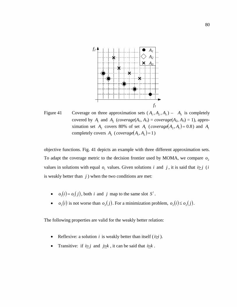
80
Figure 41 Coverage on three approximation sets ( 1A , 2A , 3A ) – 3A is completely
covered by 1A and 2A (coverage(A1, A3) = coverage(A2, A3) = 1), appro-ximation set 2A covers 80% of set 1A ( ( ) 8.0, 12 =AAcoverage ) and 1A completely covers 2A ( ( ) 1, 21 =AAcoverage )
objective functions. Fig. 41 depicts an example with three different approximation sets.
To adapt the coverage metric to the decision frontier used by MOMA, we compare 2o
values in solutions with equal 1o values. Given solutions i and j , it is said that ji ( i
is weakly better than j ) when the two conditions are met:
• ( ) ( )joio 11 = , both i and j map to the same slot lS .
• ( )io2 is not worse than ( )jo2 . For a minimization problem, ( ) ( )joio 22 ≤ .
The following properties are valid for the weakly better relation:
• Reflexive: a solution i is weakly better than itself ( ii ).
• Transitive: if ji and kj , it can be said that ki .
f1
f2
A2
A1
A3

81
Thus, ),( BAcoverage with MOMA indicates the fraction of solutions in B that have at
least one weakly better solution in A .
Later, Zitzler et al. demonstrated in [72] a coverage-based comparison method for
approximation sets that detects when A is better than B ( BA ). An approximation set
A is better than B when 1),( =BAcoverage and BA ≠ . In Fig. 41, sets 1A and 2A are
better than 3A , and set 1A is better than 2A . The coverage metric may also be used to
measure the improvement in two consecutive generations, tP and 1+tP . For each
generation t , there is a set of best solutions tB , the current Pareto front for NSGA-II
and the decision frontier for MOMA.
Given tB and 1+tB , NSGA-II and MOMA will either improve solutions in the
population and tt BB 1+ , or no improvement will be achieved and tt BB =+1 . When
there is solution improvement, set tB is not able to cover the entire set 1+tB and
( ) 1, 1 <+tt BBcoverage . If there is no solution improvement ( tt BB =+1 ), then tB covers
the entire set 1+tB and ( ) 1, 1 =+tt BBcoverage (the two sets are equal), thus the
improvement between two consecutive generations is defined in (5.1), which calculates
the fraction of individuals in 1+tB that have been improved in comparison to tB .
( ) ( )11 ,1, ++ −= tttt BBcoverageBBtimprovemen (5.1)
5.2 Stopping MOGAs
To halt the optimization process, we assume that (5.1) is capable to measure the
improvement between two consecutive generations. The concept of MOGAs indicates
that the population will evolve through generations until it reaches a good approximation
set and is unable to further improve solutions. It is desirable to detect this moment and

82
stop the optimization process regardless of the mg value set. Thus, the ideal MOGA
optimizes solutions and improve them through generations while 0>timprovemen , until
it finally converges. After this generation stopt , the MOGA is unable to improve
solutions and 0=timprovemen , as the solution set is no further improved.
However, it was observed on experimental data that both MOMA and NSGA-II will
often go through cycles where the algorithm takes some generations to actually improve
the approximation set. Hence, measuring the improvement between two consecutive
generations is not enough to detect the generation at which the algorithm should stop.
For a fair tracking of solution improvement, the improvement rate at generation t ( tir )
is calculated in (5.2) as the average improvement in the last w generations, mgw <<1 .
( )
w
BBtimprovemenir
t
wtwti
ii
t∑
−
>−=
+
=
1
,
1, (5.2)
Choosing an incorrect w value may stop the algorithm before convergence. Fig. 42
demonstrates the effect with two different w values. A low w value ( w =10) indicates
that the algorithm stopped improving ( 0tir = ) earlier, whereas a suitable value ( w =41)
will let the algorithm explore more solutions and find the true stopping generation.
At the end of each generation wtt >, , the tir value is evaluated and the optimization
process is stopped at generation stopt either if irt minir stop ≤ , a minimum improvement rate
threshold, or if mgtstop = . The stopping criterion introduces two new parameters to the
optimization process, w and crmin . It is desirable to have both good convergence and a
good spread of solutions in the approximation set, hence it is adequate to have
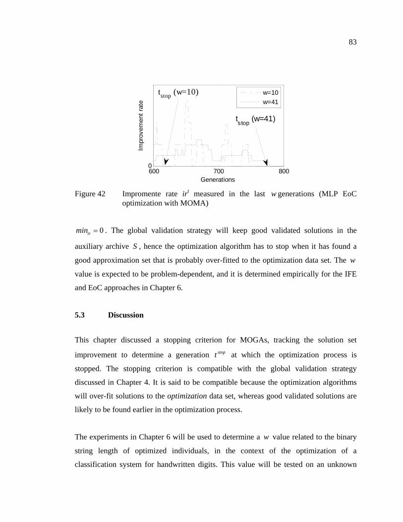
83
0irmin = . The global validation strategy will keep good validated solutions in the
auxiliary archive S , hence the optimization algorithm has to stop when it has found a
good approximation set that is probably over-fitted to the optimization data set. The w
value is expected to be problem-dependent, and it is determined empirically for the IFE
and EoC approaches in Chapter 6.
5.3 Discussion
This chapter discussed a stopping criterion for MOGAs, tracking the solution set
improvement to determine a generation stopt at which the optimization process is
stopped. The stopping criterion is compatible with the global validation strategy
discussed in Chapter 4. It is said to be compatible because the optimization algorithms
will over-fit solutions to the optimization data set, whereas good validated solutions are
likely to be found earlier in the optimization process.
The experiments in Chapter 6 will be used to determine a w value related to the binary
string length of optimized individuals, in the context of the optimization of a
classification system for handwritten digits. This value will be tested on an unknown
600 700 8000
Generations
Impr
ovem
ent r
ate
w=10w=41
tstop (w=10)
tstop (w=41)
Figure 42 Impromente rate irt measured in the last w generations (MLP EoC
optimization with MOMA)

84
problem in Chapter 7, using the approach to optimize a classification system for
uppercase letters.
The scope of this thesis is limited to the optimization of classification systems, however,
the proposed approach may also be used with traditional Pareto-based MOGAs on
different problems. Future experiments will verify this possibility, also working with
real coded individuals.

CHAPTER 6
VALIDATION EXPERIMENTS ON ISOLATED HANDWRITTEN DIGITS
Once the classification system optimization approach is defined, the next step is to
verify the chosen optimization algorithms to each optimization stage. Thus, this section
experiments the approach with both zoning operators and optimization algorithms. The
goal is to define the most appropriate zoning operator and the most performing
algorithm for each optimization stage, in order to reduce processing time while keeping
solution quality.
Tests are performed using isolated handwritten digits extracted from the NIST-SD19
database [16], a comprehensive database with more than 300000 handwritten digits
samples for optimization and testing. This large database size allows for relevant
statistical analysis when comparing optimization algorithms and zoning operators.
Complete results for these statistical analysis are detailed in the Appendix 2, whereas
this section borrows these test results to present conclusions.
6.1 Experimental Protocol
The tests indicated in Fig. 43 are performed to verify the impact of over-fit and the
previously discussed methodology to optimize classification systems. They are
performed with both NSGA-II and MOMA for comparison purposes. First, the IFE
methodology is solved to obtain the representation set IFERS (the auxiliary archive S ).
For NSGA-II, S is a Pareto front, while for MOMA, IFERS is a set of lSmax fronts.
These sets are used to train the classifier sets PDK and MLPK using the PD and MLP
classifiers (the PD classifier is included for comparison purposes). For a single classifier
system, the most accurate classifiers PDPD KSI ∈ and MLPMLP KSI ∈ are selected. EoCs

86
Figure 43 Experimental overview – the classification system optimization approach
is tested in two stages, IFE and the EoC methodologies are replicated 30 times for statistical analysis, and experimentation on FSS is performed once, due to the processing time required (the PD classifier is tested only during the first stage, whereas the MLP classifier is tested in both)
are then created with PDK and MLPK , producing PDSE and MLPSE . To further compare
NSGA-II and MOMA, an EoC is created with NSGA-II using IFERS optimized by
MOMA, producing PDES ′ and MLPES ′ . These tests are performed 30 times for meaningful
statistical analysis. Then, the FSS approach further refines solution MLPSI with both
MLP classifier
EoCOptimization
Classifierselection
SIPD
Classifierselection
FSSCoarse grain
FSSFine grain
FSSFine grain
EoCOptimization
process is embeddedin these experiments.
: classifier selection
RSIFE
IFE
SEMLP
PD classifier
SEPD
KPD
KMLP
SC
SIMLP
SF
SF
30 replications

87
NSGA-II and MOMA. Because of the processing time required for each FSS experiment
(1 to 3 days), the FSS approach is limited to a single run. Two different FSS scenarios
are analyzed: the traditional FSS approach optimizes MLPSI directly with the fine grain
FSS to obtain FS ′ ; then, both FSS levels are applied on MLPSI to obtain SC and SF .
The two scenarios are compared to determine whether or not the two-level FSS approach
is better than traditional MOGA-based FSS.
To demonstrate solution over-fit related to the MOGA optimization process, the
experiments are analyzed in three situations. First, no validation strategy is used and
solutions are selected based only on the optimization data set accuracy. Next, candidate
solutions are validated in the last generation with the selection data set. Finally, solutions
are validated in all generations with the global validation strategy using the selection
data set. The three approaches are compared to demonstrate which produces the best
results.
The disjoint data sets in Table V are used in the experiments, which are isolated
handwritten digits extracted from NIST-SD19. Except for atest and btest , observations
for each class are uniformly distributed in each data set. MLP hidden nodes are
optimized as feature set cardinality fractions in the set { }6.0,55.0,50.0,45.0,4.0=f .
MLP classifier training is performed with the training data set, while the PD classifier is
trained with the smaller training’ data set, to implement a computationally efficient
wrapper approach for IFE. The remaining data sets are used with both classifiers. The
validation data set is used to adjust the classifier parameters (MLP hidden nodes and PD
hyper planes). The wrapper approach is performed with the optimization data set, and
the selection data set is used to validate candidate solutions (global validation and
validation at the last generation). Solutions are compared with atest and btest , data sets

88
Table V
Handwritten digits data sets extracted from NIST-SD19
Database Size Origin Sample range training 150000 hsf_0123 1 to 150000 training’ 50000 hsf_0123 1 to 50000 validation 15000 hsf_0123 150001 to 165000
optimization 15000 hsf_0123 165001 to 180000 selection 15000 hsf_0123 180001 to 195000
testa 60089 hsf_7 1 to 60089 testb 58646 hsf_4 1 to 58646
unknown to the resulting solutions. It is known that btest is more difficult to classify
than atest [16], hence the robustness of the resulting solutions are tested on two different
levels of classification complexity.
Rejection strategies are applied on the best solutions obtained in each optimization stage.
The experimental data are also used to empirically determine the w value and validate
the stopping criterion with the global validation strategy. The 30 replications with the
IFE and EoC methodologies are divided into two groups. The first group of 10 random
replications is used to empirically estimate the w values and to relate w to the binary
string length. The second group, with the 20 remaining replications, is then used to
validate the stopping criterion. For each replication, the criterion is verified if the
validated solutions are the same as they are when the traditional maximum generation
number ( mg ) approach is used. The FSS experimental data are used to further validate
the relation between w and the binary string length ( L ).
The parameters used with MOMA are the following: crossover probability is set to
%80=cp , and mutation is set to Lpm /1= , where L is the length of the mutated binary
string [90]. The maximum number of generations is set to 1000=mg for all
experiments to study the impact of the w value, and the local search will look for 1=n

89
neighbors during 3=NI iterations, with deviation %0=a . Each slot in the archive S is
allowed to store 5=lSmax solutions. These parameters were determined empirically in
Chapter 3. The same parameters ( %80=cp , Lpm /1= and 1000=mg ) are used for
NSGA-II. Population size depends on the optimization problem. To optimize the zoning
operator, the population size is 64=m , while to optimize FSS, we use 100=m to keep
processing time reasonable. For the EoC optimization, 166=m is used with IFERS
optimized by MOMA ( m is twice IFERS ), and 32=m for IFERS optimized by NSGA-
II. Individual initialization is performed in two steps for both optimization algorithms.
The first step creates one individual for each possible cardinality value. For IFE and FSS
optimization, one individual associated to each possible zone number is added, while for
EoC optimization, one individual is added for each possible EoC cardinality. The second
step completes the population with individuals initialized with a Bernoulli distribution.
Experiments are conducted on a Beowulf cluster with 25 nodes using Athlon XP 2500+
processors with 1GB of PC-2700 DDR RAM (333MHz FSB). The optimization
algorithms were implemented using LAM MPI v6.5 in master-slave mode with a simple
load balance. PD vote and MLP output calculations were performed once in parallel
using a load balance strategy, and results were stored in files to be loaded into memory
for the EOC optimization process.
All tests replicated 30 times were subjected to a multiple comparison test. A Kruskal-
Wallis nonparametric test is used to test the equality of mean values, using bootstrap to
create the confidence intervals from the 30 observations in each sample. The conclusions
presented regarding the validation strategies and the algorithm comparison were
obtained with a confidence level of 95% ( 05.0=α ). Further details on these tests are
found in the Appendix 2.

90
6.2 Divider Zoning Experimental Results
This section presents and discusses results obtained for handwritten digits using the
divider zoning operator, and is divided in four subsections. The first details results for
the IFE and EoC optimization, followed by a subsection that presents results for the FSS
optimization. The third subsection verifies the proposed stopping criterion on the
experimental data. Finally, the last subsection presents conclusions related to the results
obtained with the divider zoning operator on handwritten digits.
6.2.1 IFE and EoC Experimental Results
The first stage optimizes the IFE and EoC methodologies in 30 replications using the
divider zoning operator. For each run, the most accurate solution is selected according to
the validation strategy used. Figs. 44 and 45 detail the error rate dispersion obtained in
these experiments for the PD and MLP classifiers respectively. Mean values and
standard deviations for these experiments are detailed in Tables VI and VII. In both
tables, validation indicates the validation strategy used, zones the solution zone number,
HN the number of nodes in the MLP hidden layer (MLP classifier results only), S the
solution cardinality in features or aggregated classifiers, and ateste and
bteste the error
rates in the atest and btest data sets. The baseline representation is included in both
tables for reference.
In terms of validation strategies, the statistical tests in Appendix 2 indicate that the
results obtained have an order relation between the validation approaches tested. Using
no validation is worse than using validation at the last generation, which in turn is worse
than using the global validation strategy. Mean error rate values in Tables VI and VII are
lower with the global validation strategy, which is also observed in Figs. 44 and 45.

91
1.9 2 2.1 2.2 2.3 2.4 2.5 2.6
SE' NSGA-II
SE NSGA-II
SI NSGA-II
SE MOMA
SI MOMA
SE' NSGA-II
SE NSGA-II
SI NSGA-II
SE MOMA
SI MOMA
SE' NSGA-II
SE NSGA-II
SI NSGA-II
SE MOMA
SI MOMA
Error rate
No
valid
atio
nG
loba
l val
idat
ion
Val
idat
ion
at th
ela
st g
ener
atio
n
(a) testa
5 5.2 5.4 5.6 5.8 6 6.2 6.4
SE' NSGA-II
SE NSGA-II
SI NSGA-II
SE MOMA
SI MOMA
SE' NSGA-II
SE NSGA-II
SI NSGA-II
SE MOMA
SI MOMA
SE' NSGA-II
SE NSGA-II
SI NSGA-II
SE MOMA
SI MOMA
Error rate
Val
idat
ion
at th
ela
st g
ener
atio
n
Glo
bal v
alid
atio
nN
o va
lidat
ion
(b) testb
Figure 44 PD error rate dispersion on 30 replications with the divider zoning operator – each solution set relates to one validation strategy tested: no validation, the traditional validation at the last generation and global validation
0.75 0.8 0.85 0.9 0.95
SE' NSGA-II
SE NSGA-II
SI NSGA-II
SE MOMA
SI MOMA
SE' NSGA-II
SE NSGA-II
SI NSGA-II
SE MOMA
SI MOMA
SE' NSGA-II
SE NSGA-II
SI NSGA-II
SE MOMA
SI MOMA
Error rate
No
valid
atio
nV
alid
atio
n at
the
last
gen
erat
ion
G
loba
l val
idat
ion
(a) testa
2.3 2.4 2.5 2.6 2.7 2.8
SE' NSGA-II
SE NSGA-II
SI NSGA-II
SE MOMA
SI MOMA
SE' NSGA-II
SE NSGA-II
SI NSGA-II
SE MOMA
SI MOMA
SE' NSGA-II
SE NSGA-II
SI NSGA-II
SE MOMA
SI MOMA
Error rate
Val
idat
ion
at th
ela
st g
ener
atio
n
Glo
bal v
alid
atio
nN
o va
lidat
ion
(b) testb
Figure 45 MLP error rate dispersion on 30 replications with the divider zoning operator – each solution set relates to one validation strategy tested: no validation, the traditional validation at the last generation and global validation

92
Table VI
PD optimization results with the divider zoning operator – mean values on 30 replications and standard deviation values (shown in parenthesis)
MOMA NSGA-II Validation Solution
Zones S ateste
bteste Zones S ateste
bteste
Baseline 6 132 2.96% 6.83% 6 132 2.96% 6.83%
PDSI 12 264 2.57%(0)
6.42%(0)
12 264 2.57% (0)
6.42%(0)
PDSE - 16.67 2.07%(0.043)
5.32%(0.121)
- 7 2.31% (0.007)
5.92%(0.015)
None
PDES ′ - - - - - 12.47 2.08% (0.042)
5.40%(0.112)
PDSI 15 330 2.18%(0)
5.47%(0)
10 220 2.44% (0)
6.14%(0)
PDSE - 22.5 2.01%(0.032)
5.17%(0.069)
- 7 2.31% (0.07)
5.91%(0.014)
Last
PDES ′ - - - - - 11.47 2.07% (0.058)
5.37%(0.114)
PDSI 15 330 2.18%(0)
5.47%(0)
15.77 346.85 2.22% (0.0001)
5.55%(0.02)
PDSE - 22.33 1.98%(0.033)
5.14%(0.056)
- 7.4 2.18% (0.063)
5.53%(0.122)
Global
PDES ′ - - - - - 24.67 2.00% (0.040)
5.19%(0.087)
Whereas these conclusions are valid for the general case, in three specific situations the
differences among validation strategies are not significant. Using MOMA with IFE
produces the same results with validation at the last generation or the global validation.
The same is observed when creating MLP EoCs with MOMA. Finally, creating EoCs
with NSGA-II will produce similar results with no validation or validation at the last
generation. The effect observed with MOMA is related to its auxiliary archive strategy,
which keeps a solution set of lSmax solutions for each possible cardinality value, and
partially removes the over-fit with the validation at the last generation. The exception
observed with NSGA-II is not relevant, as the global validation strategy is better. The
experimental results associated to the tests in Appendix 2 indicate that the global
validation strategy is better for both the IFE and EoC methodologies, as the impact of
over-fit on solutions is not known a priori.

93
Table VII
MLP optimization results with the divider zoning operator – mean values on 30 replications and standard deviation values (shown in parenthesis)
MOMA NSGA-II Validation Solution
Zones HN S ateste
bteste Zones HN S ateste
bteste
Baseline 6 60 132 0.91% 2.89% 6 60 132 0.91% 2.89%
MLPSI 8 97 176 0.93%(0)
2.84%(0)
6 70 132 0.98%(0)
2.81%(0)
MLPSE - - 10.07 0.78%(0.017)
2.44%(0.037)
- - 4.73 0.88%(0.037)
2.61% (0.081)
None
MLPES ′ - - - - - - - 6.8 0.77%(0.015)
2.41%(0.037)
MLPSI 15 132 330 0.82% (0)
2.51%(0)
12 132 264 0.91%(0)
2.56%(0)
MLPSE - - 16.23 0.76%(0.012)
2.37%(0.042)
- - 4.77 0.85%(0.015)
2.52%(0.040)
Last
MLPES ′ - - - - - - - 4.9 0.77%(0.016)
2.42%(0.034)
MLPSI 15 132 330 0.82% (0)
2.51%(0)
13.67 129.32 300.6 0.83%(0.013)
2.52%(0.018)
MLPSE - - 10.33 0.77%(0.017)
2.35%(0.030)
- - 4.5 0.79%(0.023)
2.47%(0.040)
Global
MLPES ′ - - - - - - - 14.13 0.76%(0.016)
2.36%(0.022)
Optimization algorithms are compared based on the results obtained with the global
validation strategy. MOMA and NSGA-II performs similarly with both classifiers to
optimize IFE (solutions PDSI and MLPSI ), selecting the zoning representation with 15
active zones depicted in Fig. 46. MOMA has no error rate dispersion with either
classifier, while NSGA-II may produce suboptimal solutions. This result is no
surprise, as MOMA was designed for the IFE methodology. Another motivation for
choosing MOMA at the IFE level is to create a more diverse IFERS set. In the 30
experimental replications, the IFERS cardinality is 82=IFERS when 5=lSmax with
MOMA, whereas with NSGA-II the cardinality is only 10=IFERS . MOMA also offers

94
Figure 46 Solution PDSI / MLPSI (15 active zones) selected with the global validation
strategy in the IFE optimization with the divider zoning operator
higher lateral diversity due to the decision frontier, and its IFERS set comprises
individuals with up to 36 active zones, while the IFERS produced by NSGA-II contains
individuals with at most 15 active zones. Classifier diversity is a key issue in optimizing
EoCs, and this is reflected on results in Tables VI and VII, where PDSE and MLPSE
optimized by NSGA-II are worse than PDES ′ and MLPES ′ optimized by NSGA-II with
IFERS optimized by MOMA.
Comparing the EoCs optimized with the global validation and using the IFERS obtained
by MOMA, there is no significant difference between MOMA and NSGA-II. Mean error
rates in Tables VI and VII are comparable according to tests performed in Appendix 2.
NSGA-II is less processor-intensive than MOMA, however, and thus it is preferable to
use NSGA-II to optimize EoCs with the IFERS obtained by MOMA.
Mean error rates in Tables VI and VII also demonstrate the accuracy improvement over
the baseline representation defined by a human expert. For a single PD classifier, the
IFE methodology reduced error rates by 26.35% on atest and 19.91% on btest . For a PD
EoC obtained by NSGA-II, error rates on atest are reduced by 32.43% based on mean
0 1 0
0
10
11
1
1

95
values and by 24.01% on btest . While improvements are proportionally higher on atest ,
numerically they are more significant on btest , where the EoC can correctly recognize
1.64% (962) more observations. This is an important improvement, as btest is more
difficult to classify than atest . For a single MLP classifier, the IFE methodology reduced
error rates by 9.89% on atest and by 13.15% on btest . For an MLP EoC obtained with
NSGA-II, improvements based on mean values are 16.48% on atest and 18.33% on
btest . Again, improvements on btest are numerically higher, as the EoC can correctly
recognize 0.53% (311) more observations in btest .
These experimental results indicate that the global validation strategy is the best
approach for both the IFE and EoC methodologies. It was also observed that it is better
to use MOMA to optimize the IFE in order to obtain a diverse set IFERS to optimize
EoCs using the NSGA-II. Selecting the best solutions with this configuration produces
the results in Tables VIII and IX. As indicated by mean values previously discussed in
Tables VI and VII, EoC cardinality is lower for the MLP EoC. Both tables details
classification accuracy with zero rejection ( maxe ) and with three fixed error rates using
rejection. Each classifier requires different rejection strategies, which are detailed in the
Appendix 3.
Figures 47 and 48 demonstrate the error-rejection curve for solutions in Tables VIII and
IX. Given these results, we observe that solutions produced by the IFE and EoC
optimization approaches outperform the baseline representation not only with zero
rejection, but with rejection as well. Classification systems optimized with both the PD
and MLP classifiers are more robust than the original baseline representation, yielding
higher accuracies. We observe that the PD EoC accuracy is boosted when using
rejection rates higher than 0%, which does not happen with the MLP EoC. This effect
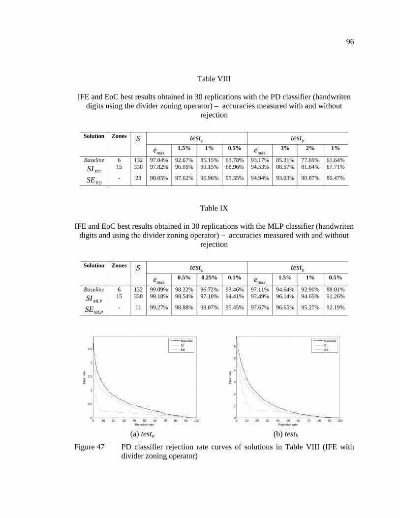
96
Table VIII
IFE and EoC best results obtained in 30 replications with the PD classifier (handwriten digits using the divider zoning operator) – accuracies measured with and without
rejection
atest btest Solution Zones S
maxe 1.5% 1% 0.5% maxe 3% 2% 1%
Baseline 6 132 97.04% 92.67% 85.15% 63.78% 93.17% 85.31% 77.69% 61.64%
PDSI 15 330 97.82% 96.05% 90.15% 68.96% 94.53% 88.57% 81.64% 67.71%
PDSE - 23 98.05% 97.62% 96.96% 95.35% 94.94% 93.03% 90.87% 86.47%
Table IX
IFE and EoC best results obtained in 30 replications with the MLP classifier (handwriten digits and using the divider zoning operator) – accuracies measured with and without
rejection
atest btest Solution Zones S
maxe 0.5% 0.25% 0.1% maxe 1.5% 1% 0.5%
Baseline 6 132 99.09% 98.22% 96.72% 93.46% 97.11% 94.64% 92.90% 88.01%
MLPSI 15 330 99.18% 98.54% 97.10% 94.41% 97.49% 96.14% 94.65% 91.26%
MLPSE - 11 99.27% 98.88% 98.07% 95.45% 97.67% 96.65% 95.27% 92.19%
0 10 20 30 40 50 60 70 80 90 1000
0.5
1
1.5
2
2.5
Rejection rate
Erro
r rat
e
BaselineSISE
(a) testa
0 10 20 30 40 50 60 70 80 90 1000
1
2
3
4
5
6
Rejection rate
Erro
r rat
e
BaselineSISE
(b) testb
Figure 47 PD classifier rejection rate curves of solutions in Table VIII (IFE with divider zoning operator)
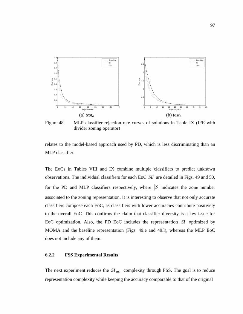
97
0 5 10 15 20 25 30 35 400
0.1
0.2
0.3
0.4
0.5
0.6
0.7
0.8
0.9
Rejection rate
Erro
r rat
e
BaselineSISE
(a) testa
0 5 10 15 20 25 30 35 40 45 500
0.5
1
1.5
2
2.5
Rejection rate
Erro
r rat
e
BaselineSISE
(b) testb
Figure 48 MLP classifier rejection rate curves of solutions in Table IX (IFE with divider zoning operator)
relates to the model-based approach used by PD, which is less discriminating than an
MLP classifier.
The EoCs in Tables VIII and IX combine multiple classifiers to predict unknown
observations. The individual classifiers for each EoC SE are detailed in Figs. 49 and 50,
for the PD and MLP classifiers respectively, where S indicates the zone number
associated to the zoning representation. It is interesting to observe that not only accurate
classifiers compose each EoC, as classifiers with lower accuracies contribute positively
to the overall EoC. This confirms the claim that classifier diversity is a key issue for
EoC optimization. Also, the PD EoC includes the representation SI optimized by
MOMA and the baseline representation (Figs. 49.e and 49.l), whereas the MLP EoC
does not include any of them.
6.2.2 FSS Experimental Results
The next experiment reduces the MLPSI complexity through FSS. The goal is to reduce
representation complexity while keeping the accuracy comparable to that of the original
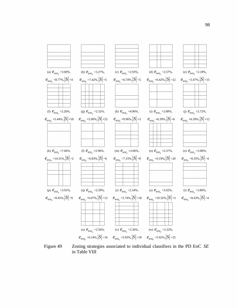
98
(a)
ateste =3.69%,
bteste =8.77%, S =4
(b)
ateste =3.27%,
bteste =7.42%, S =5
(c)
ateste =2.93%,
bteste =6.74%, S =5
(d)
ateste =2.57%,
bteste =6.42%, S =12
(e)
ateste =2.18%,
bteste =5.47%, S =15
(f)
ateste =2.26%,
bteste =5.44%, S =18
(g)
ateste =2.32%,
bteste =5.90%, S =25
(h)
ateste =4.96%,
bteste =9.96%, S =3
(i)
ateste =2.88%,
bteste =6.39%, S =6
(j)
ateste =2.72%,
bteste =6.39%, S =12
(k)
ateste =7.66%,
bteste =14.31%, S =2
(l)
ateste =2.96%,
bteste =6.83%, S =6
(m)
ateste =3.06%,
bteste =7.33%, S =8
(n)
ateste =2.37%,
bteste =6.19%, S =20
(o)
ateste =3.80%,
bteste =8.35%, S =4
(p)
ateste =3.91%,
bteste =8.45%, S =9
(q)
ateste =2.59%,
bteste =6.07%, S =12
(r)
ateste =2.34%,
bteste =5.74%, S =18
(s)
ateste =5.02%,
bteste =10.32%, S =3
(t)
ateste =3.86%,
bteste =8.43%, S =4
(u)
ateste =2.56%,
bteste =6.14%, S =16
(v)
ateste =2.36%,
bteste =5.93%, S =18
(w)
ateste =2.32%,
bteste =5.92%, S =25
Figure 49 Zoning strategies associated to individual classifiers in the PD EoC SE in Table VIII

99
(a)
ateste =0.98%,
bteste =2.81%, S =6
(a)
ateste =0.90%,
bteste =2.80%, S =8
(a)
ateste =0.83%,
bteste =2.53%, S =15
(a)
ateste =0.84%,
bteste =2.50%, S =18
(a)
ateste =0.93%,
bteste =2.58%, S =10
(a)
ateste =0.97%,
bteste =3.23%, S =5
(a)
ateste =0.83%,
bteste =2.53%, S =15
(a)
ateste =0.82%,
bteste =2.54%, S =20
(a)
ateste =0.92%,
bteste =2.87%, S =6
(a)
ateste =0.95%,
bteste =2.76%, S =10
(a)
ateste =0.89%,
bteste =2.55%, S =15
Figure 50 Zoning strategies associated to individual classifiers in the MLP EoC SE in Table IX
MLPSI . Table X details the solutions obtained in the FSS optimization experiment with
the use of all validation strategies. In this table, validation is the validation strategy used,
zones the number of active zones, HN the number of MLP hidden nodes, S the
representation cardinality (feature number) and ateste and
bteste the error rates in the atest
and btest data sets. The table also includes the baseline representation and the original
MLPSI representation optimized by IFE for comparison purposes.
FSS results also confirm the need for global validation in classification system
optimization. Solutions selected with global validation are more accurate than those

100
Table X
FSS optimization results with the divider zoning operator – best values from a single replication
MOMA NSGA-II Validation Solution
Zones HN S ateste
bteste Zones HN S ateste
bteste
Baseline 6 60 132 0.91% 2.89% 6 60 132 0.91% 2.89%
MLPSI 15 132 330 0.82% 2.51% 15 132 330 0.82% 2.51%
FS ′ 15 136 301 0.86% 2.56% 15 134 296 0.85% 2.64%
SC 15 117 293 0.85% 2.59% 15 149 298 0.85% 2.61% None
SF 15 112 280 0.87% 2.59% 15 122 243 0.85% 2.55%
FS ′ 15 123 307 0.82% 2.52% 15 134 296 0.85% 2.64%
SC 15 171 285 0.89% 2.56% 15 149 298 0.85% 2.61% Last
SF 15 148 269 0.86% 2.64% 15 122 243 0.85% 2.55%
FS ′ 15 161 321 0.82% 2.46% 15 144 318 0.83% 2.51%
SC 15 130 322 0.79% 2.53% 15 122 306 0.83% 2.54% Global
SF 15 159 318 0.82% 2.47% 15 181 301 0.83% 2.44%
selected with other strategies. The two-level FSS approach produces a solution SF with
a smaller feature set than FS ′ , produced with the traditional single-level FSS approach.
Both MOMA and NSGA-II produced a solutions SC , SF and FS ′ that are comparable
in terms of accuracy, but NSGA-II produced smaller feature sets. Reducing complexity
also improved accuracy on btest , which is higher in comparison with that of MLPSI . This
improvement is associated with the higher generalization power of smaller
representations. NSGA-II also reduced the SI cardinality from 330 features to 301
features in SF , a reduction of 8.79%. It can be said that IFE optimizes representations
with a small number of correlated features, and thus FSS is not capable of removing a
higher number of features, as these are actually required for classification. Neither
algorithm optimized solutions with missing parts. All FSS solutions have 15 active
zones as the original representation SI .
Considering this single run and the required processing time, NSGA-II is more adequate
than MOMA to reduce feature set cardinality. The solutions obtained with NSGA-II and

101
global validation are detailed in Table XI, comparing classification accuracy without
rejection ( maxe ) and with fixed error rates with rejection. Error-rejection curves for
classifiers in Table XI are detailed in Fig. 51. The rejection strategy was proposed by
Fumera in [92], which is further discussed in the Appendix 3. The error-rejection curve
of the original solution SI is comparable to the solutions with reduced feature sets
obtained with the NSGA-II ( SC , SF and FS ′ ). Thus, FSS solutions performance with
the rejection Table XI is comparable to the original SI solution, attaining the goal to
reduce feature set complexity while keeping classification accuracy. It was demonstrated
in Fig. 48 that solution SI outperforms the baseline representation when using rejection,
thus the same can be said for the solutions obtained through the FSS methodology.
6.2.3 Stopping Criterion Experimental Results
The last experiment uses the 30 IFE and EoC experimental replications to verify the
proposed stopping criterion when using the global validation strategy. A set of 10
random replications is selected to verify at which generation the optimization algorithms
have converged to a good approximation set considering the global validation strategy.
Table XI
MLP classifier FSS solutions obtained with NSGA-II and the divider zoning operator – classification accuracies measured with and without rejection
atest btest Solution Zones S
maxe 0.5% 0.25% 0.1% maxe 1.5% 1% 0.5%
Baseline 6 132 99.09% 98.22% 96.72% 93.46% 97.11% 94.64% 92.90% 88.01% SI 15 330 99.18% 98.54% 97.10% 94.41% 97.49% 96.14% 94.65% 91.26%
SC 15 306 99.17% 98.43% 96.43% 93.57% 97.49% 96.00% 94.40% 91.14%
SF 15 301 99.17% 98.55% 96.62% 94.03% 97.46% 96.28% 94.66% 91.77%
FS ′ 15 318 99.17% 98.46% 97.00% 94.17% 97.56% 96.12% 94.78% 91.32%

102
0 5 10 15 20 25 30 35 400
0.1
0.2
0.3
0.4
0.5
0.6
0.7
0.8
0.9
Rejection rate
Erro
r rat
eSISCSFSF'
(a) testa
0 5 10 15 20 25 30 35 400
0.5
1
1.5
2
2.5
Rejection rate
Erro
r rat
e
SISCSFSF'
(b) testb
Figure 51 MLP classifier rejection rate curves of NSGA-II solutions obtained with global validation in Table XI
Based on this value, a w estimate is calculated. A simple relation was established
between the problem complexity and w when 0irmin = . Given binary string length L ,
it is sufficient to have 2/Lw = to verify with 0irmin = that the algorithm stopped
improving solutions. The remaining 20 replications are used to validate the selected w
value. Table XII demonstrates w values for the optimized problems and the mean
average stopping generation stopt calculated for both NSGA-II and MOMA in these 20
replications. The table also includes the standard deviation associated to the stopt values
for these experiments.
The results in Tables VI and VII are the same when either the traditional stopping
criterion (maximum generation count) or the proposed stopping criterion is used. The
auxiliary archive S keeps good validated solutions, even when the population is over-
fitted to the optimization data set. Therefore, the proposed stopping criterion is efficient
in the context of classification system optimization and the global validation strategy.
The stopping criterion may reduce processing time, as the optimization algorithm stops
after it has converged to a good approximation set. The approach is efficient in this

103
Table XII
Divider zoning operator w values and calculated stopping generation (standard deviation values are shown in parenthesis)
MOMA NSGA-II Process
w ( 2/L ) stopt w ( 2/L )
stopt
SI 5 11 (2.881)
5 11 (2.266)
PDSE 41 904 (127.327)
5 12 (2.712)
PDES ′ - - 41 60 (14.552)
MLPSE 41 627 (136.178)
5 13 (2.806)
MLPES ′ - - 41 125 (27.995)
FS ′ 165 1000 165 1000
SC 23 167 23 79
SF 161 1000 153 873
context because validated solutions are archived in S , thus the optimization algorithm
may over-fit solutions during some generations with no loss of solution quality.
The stopping criterion is also validated with the FSS experiments, and the results are
indicated in Table XII. Standard deviation values for the FSS experiments are not
provided as they were performed only once. The coarse grain FSS optimization is the
smaller problem, with a 45-bit binary string to encode the solution, and both MOMA
and NSGA-II converge earlier than the maximum set generations ( 1000=mg ). By
contrast, the fine grain FSS optimization is a considerably larger problem, with binary
strings ranging between 306 and 330 bits. We observe that the optimization algorithms
do not converge before the maximum number of generations mg , except for SF
optimized by NSGA-II (which has the smaller bit string). These results indicate the need
for larger populations or a higher mg value for the fine grain FSS problem. Results in
Table X are also the same with the traditional stopping criterion (maximum generation
count) or with the proposed stopping criterion based on solution improvement. Hence

104
the estimated value 2/Lw = is validated on a set of unseen PR approaches based on
MOGAs with binary encoded individuals.
6.2.4 Experimental Results Discussion
On all optimization problems, it was observed that MOMA explored a higher number of
unique solutions, as it optimizes the complete decision frontier and uses a local search
approach to better explore solutions. This approach allowed MOMA to find a better
IFERS set with the IFE methodology. The drawback is that MOMA uses more
processing time, and NSGA-II offers a better compromise between solution quality and
processing time for the EoC and FSS methodologies. Another observation is that
tracking the improvement rate indicated the need to adjust the optimization parameters
in the FSS problems, which is usually overlooked when stopping the optimization
algorithm based solely on the maximum number of generations. Finally, solutions
obtained with the proposed approach to optimize classification systems outperformed
the baseline representation with the divider zoning operator.
6.3 Hierarchical Zoning Experimental Results
The same test set is repeated with the hierarchical zoning operator, thus, this section is
also divided in four subsections. First the results for the IFE and EoC optimization are
detailed, followed by a subsection that presents results for the FSS optimization. The
third subsection verifies the proposed stopping criterion on the experimental data.
Finally, the last subsection presents conclusions related to the results obtained with the
hierarchical zoning operator on handwritten digits.
6.3.1 IFE and EoC Experimental Results
The first experimental set performed with the hierarchical zoning operator optimizes the
IFE and EoC methodologies in 30 replications, as indicated in Fig. 43. The most

105
accurate solution is selected in each run according to the validation strategy used. Figs.
52 and 53 detail the error rate dispersion obtained in these experiments for the PD and
MLP classifiers respectively. Mean values and standard deviations for these experiments
are detailed in Tables XIII and XIV. In both tables, validation indicates the validation
strategy used, zones the solution zone number, HN the number of nodes in the MLP
hidden layer (MLP classifier results only), S the solution cardinality in features or
aggregated classifiers, and ateste and
bteste the error rates in the atest and btest data sets.
The baseline representation is included in both tables for reference.
Unlike the divider zoning operator, the IFE with the hierarchical zoning operator was
not able to outperform the baseline representation with both PD and MLP classifiers.
Thus, the IFE using the divider zoning operator is more powerful to optimize
representations for single classifier systems as it was able to outperform a solution
3 3.05 3.1 3.15 3.2 3.25 3.3 3.35 3.4 3.45
SE' NSGA-II
SE NSGA-II
SI NSGA-II
SE MOMA
SI MOMA
SE' NSGA-II
SE NSGA-II
SI NSGA-II
SE MOMA
SI MOMA
SE' NSGA-II
SE NSGA-II
SI NSGA-II
SE MOMA
SI MOMA
Error rate
Val
idat
ion
at th
ela
st g
ener
atio
n
Glo
bal v
alid
atio
nN
o va
lidat
ion
(a) testa
7.2 7.4 7.6 7.8 8 8.2
SE' NSGA-II
SE NSGA-II
SI NSGA-II
SE MOMA
SI MOMA
SE' NSGA-II
SE NSGA-II
SI NSGA-II
SE MOMA
SI MOMA
SE' NSGA-II
SE NSGA-II
SI NSGA-II
SE MOMA
SI MOMA
Error rate
Val
idat
ion
at th
ela
st g
ener
atio
n
No
valid
atio
nG
loba
l val
idat
ion
(b) testb
Figure 52 PD error rate dispersion on 30 replications with the hierarchical zoning operator – each solution set relates to one validation strategy tested: no validation, validation at the last generation and global validation

106
0.96 0.98 1 1.02 1.04 1.06 1.08 1.1 1.12 1.14
SE' NSGA-II
SE NSGA-II
SI NSGA-II
SE MOMA
SI MOMA
SE' NSGA-II
SE NSGA-II
SI NSGA-II
SE MOMA
SI MOMA
SE' NSGA-II
SE NSGA-II
SI NSGA-II
SE MOMA
SI MOMA
Error rate
No
valid
atio
nV
alid
atio
n at
the
last
gen
erat
ion
G
loba
l val
idat
ion
(a) testa
2.95 3 3.05 3.1 3.15 3.2 3.25 3.3
SE' NSGA-II
SE NSGA-II
SI NSGA-II
SE MOMA
SI MOMA
SE' NSGA-II
SE NSGA-II
SI NSGA-II
SE MOMA
SI MOMA
SE' NSGA-II
SE NSGA-II
SI NSGA-II
SE MOMA
SI MOMA
Error rate
No
valid
atio
nV
alid
atio
n at
the
last
gen
erat
ion
G
loba
l val
idat
ion
(b) testb
Figure 53 MLP error rate dispersion on 30 replications with the hierarchical zoning operator – each solution set relates to one validation strategy tested: no validation, validation at the last generation and global validation
defined by a human expert. We will see later that the use of a rejection strategy will
improve performance, however, with high rejection rates, whereas the divider zoning
operator performed better with lower rejection rates. The optimized EoCs are
comparable to the original baseline representation, and the use of a rejection strategy
later will improve performance, especially for the PD EoC. However, their
computational cost is much higher than a single classifier for the baseline representation.
Therefore, the first conclusion in this section is that the divider zoning operator
performed better than the hierarchical zoning operator with isolated handwritten digits.
Considering the validation strategies, the hierarchical zoning operator results indicate
that this zoning operator is less prone to over-fit than the divider zoning operator. For
both MOMA and NSGA-II the IFE produced the same representation in all 30 runs,
regardless of the validation strategy used. Mean error rates for EoCs optimized by

107
Table XIII
PD optimization results with the hierarchical zoning operator – mean values on 30 replications and standard deviation values (shown in parenthesis)
MOMA NSGA-II Validation Solution
Zones S ateste
bteste Zones S ateste
bteste
Baseline 6 132 2.96% 6.83% 6 132 2.96% 6.83%
PDSI 11 242 3.46%(0)
8.30%(0)
11 242 3.46% (0)
8.30%(0)
PDSE - 16.97 3.09%(0.037)
7.31%(0.058)
- 8 3.28% (0)
7.68%(0)
None
PDES ′ - - - - - 12.77 3.12% (0.021)
7.39%(0.084)
PDSI 11 242 3.46%(0)
8.30%(0)
11 242 3.46% (0)
8.30%(0)
PDSE - 15.47 3.07%(0.021)
7.3%(0.042)
- 8 3.28% (0)
7.68%(0)
Last
PDES ′ - - - - - 12.77 3.12% (0.040)
7.39%(0.099)
PDSI 11 242 3.46%(0)
8.30%(0)
11 242 3.46% (0)
8.30%(0)
PDSE - 14.46 3.06%(0.036)
7.3%(0.082)
- 7.33 3.27% (0.046)
7.7%(0.064)
Global
PDES ′ - - - - - 13.7 3.09% (0.034)
7.33%(0.102)
MOMA in Tables XIII and XIV are significantly lower with validation at the last
generation and the global validation strategy, as indicated by the statistical tests in the
Appendix 2. The same tests indicate that EoCs optimized by NSGA-II and IFERS
obtained with MOMA have significantly lower error rates when global validation is
used, following the trend observed with the divider zoning operator in the previous
section. This confirms the conclusion in the previous section that when the impact of
over-fit is not known a priori, it is better to use the global validation strategy as it
provides better results on over-fit prone problems. When the problem is not prone to
over-fit, it has been demonstrated that global validation produces comparable solutions.
Thus, the remainder of this section will consider solutions using the global validation for
analysis of single classifiers and EoCs. Whereas the hierarchical zoning operator was
unable to outperform the baseline representation, the results still indicate accuracy
improvements when optimizing EoCs.

108
Table XIV
MLP optimization results with the hierarchical zoning operator – mean values on 30 replications and standard deviation values (shown in parenthesis)
MOMA NSGA-II Validation Solution
Zones HN S ateste
bteste Zones HN S ateste
bteste
Baseline 6 60 132 0.91% 2.89% 6 60 132 0.91% 2.89%
MLPSI 11 134 242 1.14%(0)
3.21%(0)
11 134 242 1.14%(0)
3.21%(0)
MLPSE - - 13.64 1% (0.017)
3.04%(0.026)
- - 4.6 1.03%(0.005)
3.06%(0.032)
None
MLPES ′ - - - - - - - 7.83 1.02%(0.025)
3.07%(0.041)
MLPSI 11 134 242 1.14%(0)
3.21%(0)
11 134 242 1.14%(0)
3.21%(0)
MLPSE - - 50.79 0.99%(0.009)
2.98%(0.038)
- - 7 1.03%(0)
3.08%(0)
Last
MLPES ′ - - - - - - - 7 1.03%(0.026)
3.07%(0.046)
MLPSI 11 134 242 1.14%(0)
3.21%(0)
11 134 242 1.14%(0)
3.21%(0)
MLPSE - - 28.18 0.99%(0.012)
2.99%(0.023)
- - 5.13 1.06%(0.017)
3.1%(0.027)
Global
MLPES ′ - - - - - - - 22.86 0.99%(0.012)
2.99% (0.030)
Error rates obtained with EoCs are significantly lower than when using the single
classifier SI (for more details, see Appendix 2). The zoning strategy associated to SI
(regardless of the validation strategy used) is detailed in Fig. 54, with 11 zones (242
features). As with the divider zoning operator, the NSGA-II was able to optimize a
better EoC when using the IFERS optimized by MOMA (producing ES ′ ), which
confirms the need for a high degree of classifier diversity to properly optimize an EoC.
As with the divider zoning operator, experimental results indicate that the global
validation strategy is the best approach for both the IFE and EoC methodologies. Again,
it was also observed that it is better to use MOMA to optimize the IFE in order to obtain
a diverse set IFERS to optimize EoCs using the NSGA-II. Selecting the best solutions
with this configuration produces the results in Tables XV and XVI. Both tables details
classification accuracy without rejection ( maxe ) and with fixed error rates obtained

109
Figure 54 Solution PDSI / MLPSI (11 active zones) selected with either validation
strategies in the IFE optimization with the hierarchical zoning operator (the individual is encoded as the patterns 04454)
Table XV
IFE and EoC best results obtained in 30 replications with the PD classifier (handwriten digits and using the hierarchical zoning operator) – Classification accuracies measured
with and without rejection
atest btest Solution Zones S
maxe 1.5% 1% 0.5% maxe 3% 2% 1%
Baseline 6 132 97.04% 92.67% 85.15% 63.78% 93.17% 85.31% 77.69% 61.64%
PDSI 11 242 96.54% 88.47% 80.72% 59.86% 91.70% 78.51% 68.88% 49.58%
PDSE - 19 96.97% 95.47% 94.02% 89.29% 92.78% 88.31% 85.50% 77.72%
Table XVI
IFE and EoC best results obtained in 30 replications with the MLP classifier (handwriten digits and using the hierarchical zoning operator) – classification accuracies measured
with and without rejection
atest btest Solution Zones S
maxe 0.5% 0.25% 0.1% maxe 1.5% 1% 0.5%
Baseline 6 132 99.09% 98.22% 96.72% 93.46% 97.11% 94.64% 92.90% 88.01%
MLPSI 11 242 98.86% 97.49% 96.05% 91.40% 96.69% 93.70% 91.90% 86.98%
MLPSE - 25 99.03% 98.34% 96.93% 94.56% 97.05% 95.11% 93.50% 89.84%

110
through rejection. Details for the rejection strategies applied are discussed in the
Appendix 3. The divider zoning operator in the previous section had MLP EoCs with
lower cardinality than PD EoCs. The hierarchical zoning operator reverse the roles, and
the best PD EoC has a lower cardinality value, which is confirmed by mean values in
Tables XIII and XIV.
Concerning the single classifier SI , it has lower performance than the baseline
representation with both the PD and MLP classifiers, even when using rejection. On the
other hand, the PD EoC PDSE outperforms the baseline representation with rejection.
The MLP EoC MLPSE is comparable to the baseline representation with rejection on
0 10 20 30 40 50 60 70 80 90 1000
0.5
1
1.5
2
2.5
3
3.5
Rejection rate
Erro
r rat
e
BaselineSISE
(a) testa
0 10 20 30 40 50 60 70 80 90 1000
1
2
3
4
5
6
7
8
9
Rejection rate
Erro
r rat
e
BaselineSISE
(b) testb
Figure 55 PD classifier rejection rate curves of solutions in Table XV (IFE with hierarchical zoning operator)
atest , and performs better than the baseline representation on btest . However, this
outperformance comes with a high processing time cost, thus the IEF and EoC
methodologies are not able to outperform the baseline representation with the
hierarchical zoning operator. Figures 55 and 56 demonstrate the error-rejection curve for
solutions in Tables XV and XVI, further confirming this analysis.
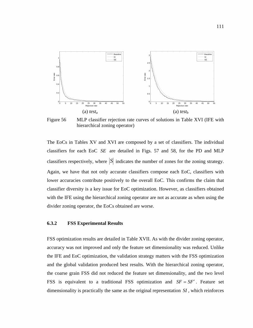
111
0 5 10 15 20 25 30 35 40 45 50 550
0.2
0.4
0.6
0.8
1
Rejection rate
Erro
r rat
eBaselineSISE
(a) testa
0 5 10 15 20 25 30 35 40 45 50 550
0.5
1
1.5
2
2.5
3
Rejection rate
Erro
r rat
e
BaselineSISE
(a) testb
Figure 56 MLP classifier rejection rate curves of solutions in Table XVI (IFE with hierarchical zoning operator)
The EoCs in Tables XV and XVI are composed by a set of classifiers. The individual
classifiers for each EoC SE are detailed in Figs. 57 and 58, for the PD and MLP
classifiers respectively, where S indicates the number of zones for the zoning strategy.
Again, we have that not only accurate classifiers compose each EoC, classifiers with
lower accuracies contribute positively to the overall EoC. This confirms the claim that
classifier diversity is a key issue for EoC optimization. However, as classifiers obtained
with the IFE using the hierarchical zoning operator are not as accurate as when using the
divider zoning operator, the EoCs obtained are worse.
6.3.2 FSS Experimental Results
FSS optimization results are detailed in Table XVII. As with the divider zoning operator,
accuracy was not improved and only the feature set dimensionality was reduced. Unlike
the IFE and EoC optimization, the validation strategy matters with the FSS optimization
and the global validation produced best results. With the hierarchical zoning operator,
the coarse grain FSS did not reduced the feature set dimensionality, and the two level
FSS is equivalent to a traditional FSS optimization and FSSF ′= . Feature set
dimensionality is practically the same as the original representation SI , which reinforces

112
(a)
ateste =15.73%,
bteste =24.00%, S =1
(b)
ateste =6.53%,
bteste =12.72%, S =2
(c)
ateste =4.22%,
bteste =9.60%, S =5
(d)
ateste =3.52%,
bteste =8.86%, S =14
(e)
ateste =6.31%,
bteste =12.59%, S =3
(f)
ateste =3.57%,
bteste =8.48%, S =12
(g)
ateste =10.49%,
bteste =17.56%, S =8
(h)
ateste =4.42%,
bteste =9.29%, S =4
(i)
ateste =3.89%,
bteste =8.39%, S =5
(j)
ateste =3.57%,
bteste =8.51%, S =11
(k)
ateste =3.80%,
bteste =9.27%, S =13
(l)
ateste =10.49%,
bteste =17.56%, S =2
(m)
ateste =3.49%,
bteste =7.90%, S =8
(n)
ateste =3.53%,
bteste =8.20%, S =11
(o)
ateste =3.75%,
bteste =8.75%, S =13
(p)
ateste =5.66%,
bteste =11.62%, S =3
(q)
ateste =4.34%,
bteste =9.09%, S =5
(r)
ateste =4.19%,
bteste =9.48%, S =6
(s)
ateste =3.79%,
bteste =8.55%, S =7
Figure 57 Zoning strategies associated to classifiers in the PD EoC SE in Table XV
the conclusion in the previous section that the IFE produces solutions adapted to the
selected feature extraction operator. The global validation strategy produced the best
results, as indicated by Table XVII.
Considering this single run and the required processing time to perform FSS, NSGA-II
is more adequate than MOMA to reduce feature set cardinality. The solutions obtained

113
(a)
ateste =1.47%,
bteste =3.95%, S =4
(b)
ateste =1.42%,
bteste =4.11%, S =5
(c)
ateste =2.23%,
bteste =4.45%, S =2
(d)
ateste =1.39%,
bteste =4.85%, S =5
(e)
ateste =1.44%,
bteste =4.13%, S =5
(f)
ateste =1.19%,
bteste =3.44%, S =6
(g)
ateste =1.26%,
bteste =3.59%, S =8
(h)
ateste =1.24%,
bteste =3.48%, S =9
(i)
ateste =1.19%,
bteste =3.27%, S =10
(j)
ateste =1.18%,
bteste =3.56%, S =7
(k)
ateste =1.24%,
bteste =3.39%, S =8
(l)
ateste =1.21%,
bteste =3.27%, S =9
(m)
ateste =1.23%,
bteste =3.29%, S =11
(n)
ateste =1.16%,
bteste =3.52%, S =12
(o)
ateste =3.1%,
bteste =6.46%, S =2
(p)
ateste =1.35%,
bteste =3.64%, S =5
(q)
ateste =1.23%,
bteste =3.38%, S =7
(r)
ateste =1.19%,
bteste =3.43%, S =9
(s)
ateste =1.27%,
bteste =3.53%, S =10
(t)
ateste =1.16%,
bteste =3.44%, S =13
(u)
ateste =1.44%,
bteste =3.76%, S =4
(v)
ateste =1.19%,
bteste =3.49%, S =7
(w)
ateste =1.3%,
bteste =3.59%, S =8
(x)
ateste =1.19%,
bteste =3.57%, S =13
(y)
ateste =1.35%,
bteste =3.98%, S =15
Figure 58 Zoning strategies associated to individual classifiers in the MLP EoC SE in Table XVI

114
Table XVII
FSS optimization results with the hierarchical zoning operator – best values from a single replication
MOMA NSGA-II Validation Solution
Zones HN S ateste
bteste Zones HN S ateste
bteste
Baseline 6 60 132 0.91% 2.89% 6 60 132 0.91% 2.89%
MLPSI 11 134 242 1.14% 3.31% 11 134 242 1.14% 3.31%
SC 11 120 218 1.28% 3.58% 11 120 218 1.28% 3.58% None
FSSF ′/ 11 115 209 1.24% 3.61% 11 90 200 1.23% 3.51%
SC 11 125 226 1.23% 3.42% 11 120 218 1.28% 3.58% Last
FSSF ′/ 11 105 209 1.23% 3.55% 11 90 200 1.23% 3.51%
SC 11 134 242 1.14% 3.31% 11 134 242 1.14% 3.31% Global
FSSF ′/ 11 131 238 1.17% 3.33% 11 120 240 1.16% 3.30%
with NSGA-II and the global validation strategy have their accuracy compared to the
baseline representation in Table XVIII, which details classification accuracy on both
atest and btest without rejection ( maxe ) and with fixed error rates using rejection (see
Appendix 3 for details on the rejection strategy). Solution SC is the same as MLPSI , thus
the equality between results (the coarse grain FSS was unable to eliminate features). The
solutions SF and FS ′ are also equal, and their performance with rejection is very close
to the original representation MLPSI .
Table XVIII
MLP classifier FSS solutions obtained with NSGA-II and the hierarchical zoning operator – classification accuracies measured with and without rejection
atest btest Solution Zones S
maxe 0.5% 0.25% 0.1% maxe 1.5% 1% 0.5%
Baseline 6 132 99.09% 98.22% 96.72% 93.46% 97.11% 94.64% 92.90% 88.01% SI 11 242 98.86% 97.49% 96.05% 91.40% 96.69% 93.70% 91.90% 86.98%
SC 11 242 98.86% 97.49% 96.05% 91.40% 96.69% 93.70% 91.90% 86.98%
FSSF ′/ 11 240 98.84% 97.45% 95.95% 91.90% 96.70% 93.74% 91.84% 86.99%

115
0 10 20 30 40 50 600
0.2
0.4
0.6
0.8
1
Rejection rate
Erro
r rat
eSISF/SF'
(a) testa
0 10 20 30 40 50 60 70 800
0.5
1
1.5
2
2.5
3
Rejection rate
Erro
r rat
e
SISF/SF'
(b) testb
Figure 59 MLP classifier rejection rate curves of NSGA-II solutions obtained with global validation in Table XVIII
The error-rejection curves in Fig. 59 confirm that solutions with reduced feature sets are
comparable to the original representation MLPSI . As the original representation MLPSI
does not outperform the baseline representation (even with rejection), it can also be said
that solutions with reduced feature sets does not outperform the baseline representation.
6.3.3 Stopping Criterion Experimental Results
The last experiment uses the 30 IFE and EoC experimental replications to verify the
proposed stopping criterion when using the global validation strategy. The procedure
used with the divider zoning operator is repeated, selecting a set of 10 random
replications to verify at which generation the optimization algorithms have converged to
a good approximation set when using the global validation strategy. Based on this value,
an estimate of w is calculated and a relation was established between the problem
complexity and w when 0irmin = . Again, given the binary string length L , it is
sufficient to have 2/Lw = to verify algorithm convergence when min 0ir = . The
remaining 20 replications are then used to validate the selected w value. Table XIX
demonstrates w values for the optimized problems and the mean average stopping
generation stopt calculated for both NSGA-II and MOMA in these 20 replications. The
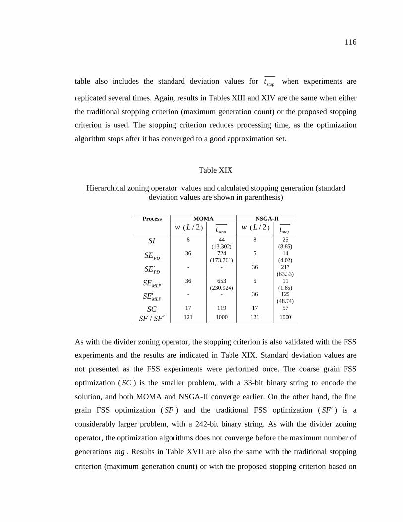
116
table also includes the standard deviation values for stopt when experiments are
replicated several times. Again, results in Tables XIII and XIV are the same when either
the traditional stopping criterion (maximum generation count) or the proposed stopping
criterion is used. The stopping criterion reduces processing time, as the optimization
algorithm stops after it has converged to a good approximation set.
Table XIX
Hierarchical zoning operator values and calculated stopping generation (standard deviation values are shown in parenthesis)
MOMA NSGA-II Process
w ( 2/L ) stopt w ( 2/L )
stopt
SI 8 44 (13.302)
8 25 (8.86)
PDSE 36 724 (173.761)
5 14 (4.02)
PDES ′ - - 36 217 (63.33)
MLPSE 36 653 (230.924)
5 11 (1.85)
MLPES ′ - - 36 125 (48.74)
SC 17 119 17 57
FSSF ′/ 121 1000 121 1000
As with the divider zoning operator, the stopping criterion is also validated with the FSS
experiments and the results are indicated in Table XIX. Standard deviation values are
not presented as the FSS experiments were performed once. The coarse grain FSS
optimization ( SC ) is the smaller problem, with a 33-bit binary string to encode the
solution, and both MOMA and NSGA-II converge earlier. On the other hand, the fine
grain FSS optimization ( SF ) and the traditional FSS optimization ( FS ′ ) is a
considerably larger problem, with a 242-bit binary string. As with the divider zoning
operator, the optimization algorithms does not converge before the maximum number of
generations mg . Results in Table XVII are also the same with the traditional stopping
criterion (maximum generation count) or with the proposed stopping criterion based on
117
solution set improvement. Hence the estimated value 2/Lw = is confirmed for the
stopping criterion.
6.3.4 Experimental Results Discussion
It was also observed with the hierarchical zoning operator that MOMA explored a higher
number of unique solutions, as it optimizes the complete decision frontier and uses a
local search approach to explore solutions. This approach allowed MOMA to find a
better IFERS set with the IFE methodology to optimize EoCs. The drawback is that
MOMA uses more processing time, and NSGA-II offers a better compromise between
solution quality and required processing time for the EoC and FSS methodologies. The
hierarchical zoning operator was unable to outperform the baseline representation,
unlike the divider zoning operator. A single classifier obtained with the IFE using the
hierarchical zoning operator was comparable to the baseline representation only with a
high rejection rate. The EoCs obtained had similar performance to the baseline
representation, and the use of rejection strategies improved their performance. However,
their computational costs are higher than that of a single classifier, and a similar
performance to the baseline representation is not enough to justify this operator. Thus, it
can be said that the hierarchical zoning operator has not the representational power to
create discriminating feature sets for this classification problem.
6.4 Discussion
This chapter assessed the proposed classification system optimization approach. Tests
were performed on isolated handwritten digits to verify zoning operators and
improvements against a baseline representation defined by a human expert. Results
demonstrated that the divider zoning operator provided better results when optimizing
classification systems, outperforming the baseline representation. The hierarchical
zoning operator was unable to optimize solutions better than the baseline representation.

118
Comparing results obtained with both zoning operators (with and without rejection), it is
clear that the divider zoning operator outperformed the hierarchical zoning operator on
these experiments.
Concerning the impact of over-fit, experiments indicate that over-fit is problem
dependant as discussed in [48]. This situation is mostly observed with the hierarchical
zoning operator. Also, it was observed that global validation guarantees that good
solutions found are preserved regardless of the over-fit impact. Thus, it is concluded that
it is safer to use global validation, as the impact of over-fit is not known a priori.
The optimization algorithms were also compared, and it was found that global validation
allows both MOMA and NSGA-II to perform similarly in the IFE task, but MOMA
produces a more diverse representation set IFERS to optimize EoCs. MOMA optimizes
the entire decision frontier, keeping a set of lSmax solutions for each feature set
dimensionality, and it was expected that its IFERS set had higher representation
diversity. On the other hand, NSGA-II performed similar to MOMA to optimize EoCs
(using IFERS optimized by MOMA) and to reduce feature set dimensionality through
FSS. The NSGA-II advantage over MOMA is the smaller processing time required to
optimize good solutions, which makes this algorithm more suitable for both EoC and
FSS optimization tasks.
Comparing results obtained in Tables VIII and IX with the divider zoning operator to
other representations in the literature, we have the following scenario. Milgram et al.
experimented with isolated handwritten digits in [93]. Using the same baseline
representation they obtained error rates of 1.35% on atest with a NN classifier and
0.63% on atest with a SVM (one against all). Correia [94] used an MLP classifier to
obtain an error rate of 1.12% on atest and 3.32% on btest . Liu and Sako [95] using the
PD classifier obtained an error rate of 8.11%, but on a different NIST-SD19 data set

119
partitioning. The results obtained by Milgram with SVM are the most interesting, as they
outperform the solutions optimized by the proposed approach, however, with a different
classifier. It has been known that SVM classifier are more discriminating than MLP
classifiers, and future works shall experiment with SVM classifiers to obtain higher
accuracies.
The next chapter will use the analysis performed in this chapter to experiment the
approach to optimize classification systems with isolated handwritten uppercase letters.
Based on results presented in this chapter, experiments with isolated handwritten
uppercase letters in the next chapter will use the following configuration. All
experiments will use the global validation to guarantee generalization power on selected
solutions. The IFE will use the divider zoning operator for its higher performance
observed with handwritten digits. MOMA will be used to optimize the IFE to produce a
diverse IFERS set, while the NSGA-II will be used for EoC and FSS optimization.
Finally, the FSS optimization process will use the proposed two-level FSS as it produced
better results with the divider zoning operator.

CHAPTER 7
EXPERIMENTS ON ISOLATED HANDWRITTEN UPPERCASE LETTERS
Chapter 6 assessed the proposed approach to optimize classification systems with
isolated handwritten digits. These experiments were verified the most performing zoning
operator for the IFE, the best validation strategy and the use of optimization algorithms.
To verify the system’s robustness on an unknown problem, an experiment with
uppercase letters is performed. This chapter discusses the experimental protocol for
these tests, presents the results and discusses them, comparing to a baseline
representation defined by a human expert.
7.1 Experimental Protocol
The tests with uppercase letters are performed as indicated in Fig. 60. Chapter 6
determined the best configuration to optimize the classification optimization system.
Unlike the experiments detailed in Chapter 6, experiments with handwritten letters only
aim to validate the classification system optimization approach, not the validation
strategies, zoning operators or optimization algorithms. Thus, experiments with
uppercase letters are performed using the following configuration:
• Global validation to select solutions through generations.
• Two-level FSS to reduce representation cardinality.
• MOMA to optimize the IFE.
• NSGA-II to optimize EoCs and FSS.
• Divider zoning operator.
The IFE methodology is applied first to obtain the representation set IFERS (the
auxiliary archive S ) with MOMA. This set is then used to train the classifier sets PDK

121
Figure 60 Experimental overview – the classification system optimization approach
is tested in two stages, the IFE and the EoC methodologies are replicated 30 times for statistical analysis, experimentation on FSS is performed once, due to the processing time required (the PD classifier is tested only during the first stage, whereas the MLP classifier is tested in both stages)
and MLPK using the PD and MLP classifiers. The most accurate classifiers
PDPDPD KSISI ∈, and MLPMLPMLP KSISI ∈, are selected for a single classifier system.
EoCs are then optimized using the NSGA-II with PDK and MLPK , producing PDSE and
MLPSE . These tests are performed 30 times for meaningful statistical analysis. The FSS
MLP classifier
EoCOptimization
Classifierselection
SIPD
Classifierselection EoC
Optimization
process is embeddedin these experiments.
: classifier selection
FSSFine grain
FSSCoarse grain
SC
SF
RSIFE
IFE
SEMLP
PD classifier
SEPD
KPD KMLP
SIMLP
30 replications

122
approach further refines solution MLPSI , reducing representation cardinality in order to
speed up the classification process. As with handwritten digits, the processing time
required for each FSS stage limits this stage to a single run using the NSGA-II.
Experiments are performed with the disjoint data sets in Table XX, which are isolated
handwritten uppercase letters extracted from NIST-SD19. The protocol to train, validate
and test classifiers is the same as in Chapter 6. MLP hidden nodes are optimized as
feature set cardinality fractions in the set { }6.0,55.0,5.0,45.0,4.0=f . MLP and PD
classifier training is performed with the training data set. The validation data set is used
to adjust the classifier parameters (MLP hidden nodes and PD hyper planes). The
wrapper approach is performed with the optimization data set, and the selection data set
is used to validate candidate solutions with global validation. Solutions are compared
with the test data set, unknown to the resulting solutions.
Table XX
Handwritten uppercase letters data sets extracted from NIST-SD19
Database Size Origin Sample range training 43160 hsf_0123 1 to 43160
validation 3980 hsf_4 1 to 3980 optimization 3980 hsf_4 3981 to 7960
selection 3980 hsf_4 7961 to 11940 test 12092 hsf_7 1 to 12092
The parameters used with MOMA are the following: the crossover probability is set to
%80=cp , and mutation probability is set to Lpm /1= , where L is the length of the
mutated binary string [90]. The local search operator will look for 1=n neighbors
during 3=NI iterations, with deviation %0=a . Each slot in the archive S is allowed
to store 5=lSmax solutions. These parameters were determined empirically during the
preliminary experiments detailed in Chapter 3. The same parameters

123
( %80=cp , Lpm /1= ) are used for NSGA-II. The maximum number of generations for
both algorithms is dynamically determined with the proposed stopping criterion, using
2/Lw = , 0irmin = and 1000=mg , which stops the algorithm when it detects that
solutions cannot be improved, or at most in 1000 generations.
Population size is problem dependent. To optimize the zoning operator, the population
size is 64=m , while to optimize FSS, we use 100=m for the coarse grain FSS and
150=m for the fine grain FSS. The later value is based on previous results obtained
with handwritten digits that indicated that a larger population is required for fine grain
FSS. For EoC optimization, 166=m is used. Individual initialization is performed in
two steps in all optimization processes. The first step creates one individual for each
possible cardinality value. For IFE and FSS optimization, one individual associated with
each possible number of zones is added, while for EoC optimization, one individual is
added for each possible EoC cardinality. The second step completes the population with
individuals initialized with a Bernoulli distribution.
As with handwritten digits, experiments are conducted on a Beowulf cluster. The cluster
has 25 nodes using Athlon XP 2500+ processors with 1GB of PC-2700 DDR RAM
(333MHz FSB). The optimization algorithms were implemented using LAM MPI v6.5
in master-slave mode with a simple load balance. PD vote and MLP output calculations
were performed once in parallel using a load balance strategy, and results were stored in
files to be loaded into memory for the EOC optimization process.
7.2 Experimental Results
This section presents and discusses results obtained for handwritten uppercase letters
using the divider zoning operator, and the algorithms selected in Chapter 6. The first
subsection details results for the IFE and EoC optimization, followed by a subsection

124
that presents results for the FSS optimization. The third subsection verifies the proposed
stopping criterion on the experimental data.
7.2.1 IFE and EoC Experimental Results
The first stage optimizes the IFE and EoC methodologies in 30 replications, using both
the PD and MLP classifiers. For each replication, solutions are validated using global
validation and the best solution found in each replication is used for comparisons.
Figures 61 and 62 indicate the test error rate dispersion of selected SI and SE
solutions for the PD and MLP classifiers. Mean error rate and standard deviation values
are detailed in Tables XXI and XXII. In both tables, zones indicates the solution zone
number, HN the number of nodes in the MLP hidden layer (MLP classifier results only),
S the solution cardinality in features or aggregated classifiers, and teste the error rate in
the test data set. The baseline representation is included in both tables for comparison
purposes.
Solution PDSI and MLPSI are the same on all 30 replications, thus mean error rate values
in Tables XXI and XXII are the actual error rate for these solutions. The zoning
strategies for these solutions are detailed in Fig. 63. Mean error rates in Tables XXI and
XXII demonstrate the accuracy improvement over the baseline representation defined by
a human expert. For a single PD classifier ( PDSI ), the IFE methodology reduced the
error rate by 21.84%. For a PD EoC ( PDSE ) the error rate was reduced by 30.11% based
on mean values. For a single MLP classifier ( MLPSI ), the IFE methodology improved
accuracy by 14.2%, and for an MLP EoC ( MLPSE ), improvements based on mean values
are of 19.60%.

125
6.2 6.4 6.6 6.8 7 7.2 7.4 7.6 7.8 8 8.2
SE
SI
Error rate
Figure 61 Uppercase letters PD error rate dispersion on 30 replications – each solution set relates to one optimization problem: IFE ( SI ) and EoC (SE) optimization
3.8 3.9 4 4.1 4.2 4.3 4.4
SE
SI
Error rate
Figure 62 Uppercase letters MLP error rate dispersion on 30 replications – each solution set relates to one optimization problem: IFE ( SI ) and EoC (SE) optimization
Table XXI
Uppercase letters PD optimization results – mean values on 30 replications and standard deviation values (shown in parenthesis)
Solution Zones S teste Baseline 6 132 9.20%
PDSI 16 352 7.19%(0)
PDSE - 14.41 6.43%(0.131)
Selecting the best solutions in Tables XXI and XXII produces the results in Tables
XXIII and XXIV, detailing classifier accuracy without rejection ( maxe ) and with fixed
error rates with the use of a rejection mechanism. As indicated by mean values

126
Table XXII
Uppercase letters MLP optimization results – mean values on 30 replications and standard deviation values (shown in parenthesis)
Solution Zones HN S teste Baseline 6 80 132 5.00%
MLPSI 10 88 220 4.29%(0)
MLPSE - - 5.23 4.02%(0.093)
0 1
01
0
11
1
01 1 1
0
0
01
11
0
(a) (b)
0
Figure 63 Solutions PDSI (a) and MLPSI (b), with 16 and 10 active zones respectively, selected with the global validation strategy in the IFE optimization
previously discussed in Tables XXI and XXII, EoC cardinality with the divider zoning
operator is lower for the MLP EoC, an effect also observed with handwritten digits in
the previous chapter. For further details on the rejection strategies used, see the
Appendix 3.
Solutions obtained with the IFE and EoC methodologies outperform the baseline
representation with and without the use of rejection strategies. PD and MLP classifier
results in Tables XXIII and XXIV are significantly better with the proposed IFE and

127
Table XXIII
IFE and EoC best results obtained in 30 replications with the PD classifier (handwritten letters and using the divider zoning operator) – accuracies measured with and without
rejection
test Solution Zones S maxe 4% 2% 1%
Baseline 6 132 90.80% 66.56% 34.30% 16.47%
PDSI 16 352 91.81% 81.44% 50.46% 21.94%
PDSE - 12 93.78% 91.01% 83.47% 75.75%
Table XXIV
IFE and EoC best results obtained in 30 replications with the MLP classifier (handwritten uppercase letters using the divider zoning operator) – Accuracies measured
with and without rejection
test Solution Zones S maxe 1.5% 1% 0.5%
Baseline 6 132 95.00% 89.07% 86.30% 82.20%
MLPSI 10 220 95.71% 90.54% 88.65% 82.51%
MLPSE - 5 96.11% 93.07% 90.64% 85.58%
EoC approaches. For both the PD and MLP classifier, EoCs are better than single
classifiers, justifying once again the use of the multiple classifier approach. Figures 64
and Figure 65 depict the error-rejection curve for these solutions, confirming this
analysis.
The EoCs in Tables XXIII and XXIV are composed by the classifier sets detailed in
Figs. 66 and 67, for the PD and MLP classifiers respectively, where S indicates the
zone number associated to the representation. Figures 66.c and 67.c indicate that one

128
0 10 20 30 40 50 60 70 80 90 1000
1
2
3
4
5
6
7
8
9
10
Rejection rate
Erro
r rat
e
BaselineSISE
Figure 64 PD classifier rejection rate curves of solutions in Table XXIII (IFE with divider zoning operator)
0 10 20 30 40 50 60 70 80 90 1000
0.5
1
1.5
2
2.5
3
3.5
4
Rejection rate
Erro
r rat
e
SISF
Figure 65 MLP classifier rejection rate curves of solutions in Table XXIV (IFE with divider zoning operator)
solution selected in the EoC have higher accuracy than PDSI and MLPSI . We verified
solutions selected with validation at the last generation and with no validation, only to
find out that PDSI and MLPSI obtained with global validation have the highest accuracy
on the test data set. We believe that the solutions in Figs. 66.c and 67.c were not found

129
due to the size of the selection data set used to validate optimized solutions. Thus, it can
be said that whereas the global validation performs better than the other validation
strategies tested, the selection data set size will impact in the global validation strategy
performance.
Again, we have that not only accurate classifiers compose each EoC, and classifiers with
lower accuracies contribute to the overall EoC performance. This follows the trend
observed with handwritten digits in the previous chapter, indicating that classifier
diversity is a key issue for EoC optimization. The PD EoC included the baseline
representation, whereas the MLP EoC included the representation SI optimized by the
IFE.
7.2.2 FSS Experimental Results
The next stage refines solution MLPSI through FSS, where the goal is to reduce
representation complexity while keeping the accuracy comparable to the original MLPSI .
Table XXV details the solutions obtained with the proposed two level FSS approach,
detailing the original classification accuracy (without rejection, maxe ) and with the use of
rejection to obtain fixed error rates (see details in the Appendix 3). In this table, zones is
the number of active zones, HN the number of MLP hidden nodes, S the representation
cardinality (feature number) and test the accuracy in the test data set, regarding the
rejection strategies or with 0 rejection. The table also includes the baseline
representation and the original MLPSI representation optimized by the IFE for
comparison purposes.
It was observed with handwritten digits in Table X that the two level FSS was not able
to remove a large number of features (reducing less than 10%). The conclusion was that

130
(a) teste =12.80%, S =3
(b) teste =9.20%, S =6
(c) teste =6.91%, S =24
(d) teste =7.56%, S =30
(e) teste =16.68%, S =2
(f) teste =12.79%, S =3
(g) teste =7.75%, S =12
(h) teste =7.78%, S =15
(i) teste =7.14%, S =25
(j) teste =7.69%, S =30
(k) teste =12.64%, S =5
(l) teste =7.70%, S =12
Figure 66 Zoning strategies associated to individual classifiers in the PD EoC SE in Table XXIII
(a) teste =4.29%,
S =10
(b) teste =5.32%,
S =6
(c) teste =4.24%,
S =8
(d) teste =4.76%,
S =10
(e) teste =4.81%,
S =5
Figure 67 Zoning strategies associated to individual classifiers in the MLP EoC SE in Table XXIV
the IFE optimized a solution MLPSI with few correlated features. This effect is also
observed with handwritten uppercase letters, and it is stronger than with
handwritten digits. The coarse grain FSS is unable to remove feature transformations,
keeping the original 220 features ( MLPSISC = ), whereas the fine grain FSS removes
only two features. These results further justify the claim that the IFE finds a zoning
strategy adapted to the feature vector.

131
Table XXV
Uppercase letters FSS optimization results, best values from a single replication (classification accuracies are measured with and without rejection)
test Solution Zones HN S
maxe 1.5% 1% 0.5%
Baseline 6 80 132 95.00% 89.07% 86.30% 82.20%
MLPSI 10 88 220 95.71% 90.54% 88.65% 82.51%
SC 10 88 220 95.71% 90.54% 88.65% 82.51%SF 10 98 218 95.73% 90.49% 88.24% 84.01%
Figure 68 demonstrates the similarity of MLPSI and SF through their error-rejection.
This is depicted by the nearly equal error-rejection curves, implying that their
performance ( SI and SF ) is equivalent when using a rejection strategy. However, it
must be noted that SF has only two less features than SI and that it is expected for both
classifiers to have similar performance.
7.2.3 Stopping Criterion Experimental Results
The stopping criterion is able to reduce processing time, as indicated in Table XXVI.
Again, the fine grain FSS process stops at the maximum number of generations
( 1000=mg ), regardless of the increased population size ( 150=m ) in comparison to the
experiments in Chapter 6. This further exposes the complexity associated to the fine
grain FSS process, which in consequence requires the exploration of a larger number of
candidate solutions for complete convergence. For the remaining optimization processes,
the stopping criterion stops the optimization process at a generation mgtt stopstop <, . The
results presented in Tables XXI and XXII provide similar improvements to those
obtained in Chapter 6, thus confirming the stopping criterion on an unknown problem.
Standard deviation values for stopt are not provided for the FSS experiments as they are
performed only once.

132
0 10 20 30 40 50 60 70 80 90 1000
0.5
1
1.5
2
2.5
3
3.5
4
Rejection rate
Erro
r rat
e
SISF
Figure 68 MLP classifier rejection rate curves of solutions in Table XXV
Table XXVI
w values and calculated stopping generation for the uppercase letters experiments (standard deviation values are shown in parenthesis)
Process w ( 2/L )stopt
SI 5 10 (2.687)
PDSE 41 204 (68.240)
MLPSE 41 124 (28.524)
SC 15 142 SF 110 1000
7.3 Discussion
This chapter assessed the approach to optimize classification systems with isolated
handwritten uppercase letters, an unknown problem to the approach to optimize
classification systems and the configuration selected in Chapter 6. Whereas the goal in

133
Chapter 6 was to find the best combination of zoning operator, optimization algorithms
and validation strategies, this chapter used the best configuration to optimize a
classification system for uppercase letters.
The main goal of the proposed approach to optimize classification systems is to adapt
classification systems to other problems. In this context, a classification system based on
the baseline representation is adapted to uppercase letters. As expected, representations
optimized for this problem are different than representations found for handwritten digits
in Chapter 6, justifying once again the approach to optimize classification systems.
Solutions found outperformed the baseline representation, originally defined for
handwritten digits, and the optimized EoCs further improved accuracy. One aspect
noticed in both experiments with digits and uppercase letters is that EoC improvements
are higher with the PD classifier. One possible explanation is that the IFE produces
solutions based on the PD classifier, and solution diversity is not as high when training
the MLPs. However, this statement cannot be verified as the processing time required to
optimize the IFE with MLPs renders this test unfeasible.
The two level FSS was not able to reduce the representation MLPSI complexity. The FSS
experiments with digits in Chapter 6 did not reduce a significant amount of features with
the divider zoning operator, and with the hierarchical zoning operator the results are
similar to those presented in this chapter. Thus, it can be said that the IFE selects a
zoning strategy adapted to the feature extraction operator, producing a representation
with few correlated features that FSS is not able to reduce to speedup the classification
stage.
Comparing the results in Tables XXIII and XXIV, we obtain the following results.
Milgram et al. used the same test data set and the baseline representation in [93],
obtaining error rates of 7.60% with a 3-NN classifier and 3.17% with a SVM classifier

134
(one against all). The result with the SVM classifier indicates that a more discriminating
classifier may improve accuracy, as the baseline representation was outperformed by the
proposed approach with the MLP classifier. A direct comparison to other works in the
literature is difficult, due to differences in the experimental protocol to test classifiers.
Thus, error rates are listed to illustrate typical accuracies with uppercase letters, not as
comparable values to the presented experimental results. Koerich in [33] used an MLP
classifier to classify handwritten letters from NIST-SD19 (both uppercase and
lowercase), obtaining an error rate of 11.90%. Oh and Suen in [25] used a modular
neural network to experiment with uppercase letters extracted from NIST-SD19,
obtaining an error rate of 9.94%.

CONCLUSIONS
This thesis proposed and assessed an approach to optimize and adapt classification
systems based on multi-objective genetic algorithms. This difficult problem has been
traditionally solved by human experts, whereas the proposed semi-automatic approach
uses the expert’s domain knowledge to create a representation set to optimize and adapt
classification systems. We have seen that this problem is difficult since the over-fit to
the optimization stage plays an important role, which is often overlooked in similar
methodologies. The choice of a suitable validation strategy was the key to find
performing solutions with good generalization power to unseen data.
A serie of experimental tests was performed to evaluate the methodologies for
optimizing classification systems with both the PD and MLP classifiers. It was observed
that IFE outperformed the traditional human expert based approach and produced a set
of diverse classifiers, which can be aggregated into an EoC for higher accuracy than a
single classifier. IFE also prototypes solutions using a computationally efficient wrapper
with the PD classifier. This wrapper approach reduces processing time and turns IFE
into a feasible approach for genetic optimization. The proposed two-level FSS
methodology outperformed the traditional one-level FSS with handwritten digits and the
divider zoning operator, producing an accurate and less complex classifier. Solutions
obtained in the FSS context had no missing parts and all zones were active. From this
statement, we conclude that missing parts are not a key issue for FSS optimization, and
that representation complexity can be measured through the feature set cardinality on
future experiments.
This thesis also demonstrated that, similar to learning algorithms, methodologies to
optimize classification systems using a wrapped classifier are prone to solution over-fit.
Validation strategies to overcome this challenge have been discussed and tested. It was
observed in some problems that the global validation is not significantly better than

136
validation at the last generation. However, since the impact of over-fit on solutions
obtained is unknown a priori, it is safer to use global validation as it guarantees solution
quality once the optimization process has been completed in all situations.
It was also demonstrated that MOMA outperforms NSGA-II for the IFE methodology
when the classification system targets EoCs. This effect is associated with the
exploratory mechanism in MOMA and its archiving strategy. The drawback is that
MOMA requires more processing power to complete the optimization process. When a
single classifier solution is desired, then NSGA-II can be used in place of MOMA. The
EoC methodology results indicate no significant advantage in accuracy for either
algorithm, and thus it was concluded that the NSGA-II is the most appropriate
optimization algorithm considering the required processing time.
As for the FSS approach, results for both MOMA and NSGA-II are comparable in
accuracy. It was also seen that the proposed two-level FSS approach may provide better
solutions in some situations. One conclusion from the experimental data is that the IFE
already produces a solution SI with few correlated features, adapted to the selected
feature extraction operator. This was better observed with uppercase letters, where the
FSS operation removed no more than 2 features. Considering the restrictions imposed by
the limited experimental data, it can be also said that NSGA-II is preferable to MOMA
in terms of required processing power. A more significant statistical analysis to verify
these statements is required, however, the processing time required currently makes this
analysis not feasible.
Finally, the experimental data were used to validate a stopping criterion adapted to
classification system optimization in the context of the global validation. The novelty of
this stopping criterion is that it takes into account not only the maximum generation
count, but the algorithm improvement rate as well. A relation between the encoded
binary string and the w parameter was empirically determined with handwritten digits

137
to monitor improvement in that context. The stopping criterion discussed is capable of
detecting convergence and halts the algorithm before the set maximum number of
generations, thereby reducing processing time while keeping solution quality. The
stopping criterion also helped verify the need to revise the population size or maximum
number of generations with the fine grain FSS optimization.
Even thought this thesis successfully proposed and tested the approach, obtaining
significant improvements in both classification accuracy and in understanding the over-
fit issue, some aspects where not developed owing to time and scope constraints. Here
we outline future directions we believe worthy of investigation:
• Evaluate different zoning operators, most specifically operators that allow zones
to overlap and do not necessarily cover the entire image.
• Optimize classification systems for other zoning based classification problems,
such as signature verification, which could benefit from the proposed semi-
automatic approach.
• Compare the MOGA based approach to other optimization algorithms, aiming to
find a better compromise between solution quality and required processing time.
• Investigate the stopping criterion with other multi-objective optimization
problems outside the pattern recognition domain, also aiming real coded
individuals, rather than working only with binary coded individuals.

APPENDIX 1
Fast elitist non-dominated sorting genetic algorithm – NSGA II

139
The Fast Elitist Non-Dominated Sorting Genetic Algorithm (NSGA-II) introduced by
Deb et al. in [63], is a second generation MOGA (as classified by Coello in [55]). This
particular algorithm is chosen as this thesis baseline MOGA, owing its known efficiency
to solve MOOPs in the literature [96, 97, 98]. The NSGA-II has also been used as a
baseline MOGA for problem specific algorithms comparison [99, 100] and in general
MOGA studies [101, 102, 103], which further justifies this choice. The main advantage
of NSGA-II lies on its elite and diversity preservation mechanisms.
The NSGA-II procedure is outlined in Fig. 69, evolving a population P of constant size
m . The offspring population mQQ tt =, is created from the parent population
mPP tt =, . Both tQ and tP populations are combined to create population
mRR tt 2, = . A non-dominated sorting is applied on tR and the new population 1+tP is
filled by solutions of different non-dominated fronts tii RFF ∈, . The process is
performed from the best to the worse front, until mPF ti >∪ +1 . At this point a
diversity metric is used to sort individuals in iF and individuals are copied to 1+tP until
mPF ti =∪ +1 . Remaining solutions in tR are rejected. This process is algorithmically
detailed in Algorithm 9.
Diversity preservation is achieved through the use of the crowding distance. Given
solution i , the crowding distance measures the perimeter of the cuboid described by the
two nearest solutions to i . The crowding distance favors solutions isolated in the
objective function space to help the algorithm to exploit that area. One advantage of
using the crowding distance is its parameter free nature, allowing the metric self
adaptation to the current population. The crowding distance assignment in Algorithm 9
is detailed in Algorithm 10. For every solution in the front F we initially assign a 0
diversity value. Next for each objective function m we rank solutions from the lowest to

140
Figure 69 NSGA-II procedure
Algorithm 9: NSGA-II algorithm Result : Population P Creates initial population 1P with m individuals
1=t ; while mgt < do QPR tt ∪= ; F =fast-non-dominated-sort ( )tR ; while mFP it ≤++1 do
itt FPP ∪= ++ 11 ; crowding-distance-assignement ( )iF ; 1+= ii ; end ( )n
iFSort ≺, ;
( )[ ]111 :1 +++ −∪= titt PNFPP ;
1+tQ =make-new-pop ( )1+tP ; 1+= tt ; end
Rt
F1
F2
F3
F4
F5Qt
Pt
Rejected
Pt +1 distancesorting
Non-dominatedsorting
Crowding

141
Algorithm 10: Crowding distance assignment Data: Front F Result : Crowding-distance vector Id
0, =∈∀ idFi ; for Mm ,,1functionobjective …= do Sort F in worse order of mf or find the sorted indices vector ),( >= mm fsortI ; Fl = ;
∞== ml
ml II
dd (set a large distance to boundary solutions);
for 1,,2 −= lj … do
minmax
11
mm
Im
Im
II ffffdd
jj
mj
mj −
−+=
−+
;
end end
the highest values, assigning to the boundary solutions a high diversity value ( ∞ ). The
remaining solutions are assigned a value calculated with the average value of the cuboid
perimeter for that objective function. Once the procedure is done, the most isolated
solutions have high diversity values, whereas close solutions have lower diversity
values.
Crossover and mutation genetic operations to create tQ are performed as usual on the
mating pool M . Selection is performed differently, using a crowded tournament
selection. This selection assumes that each solution in tP has two properties, the non-
dominated rank ir in the population and the local crowding distance id . It creates the
mating pool M from tP by taking pairs of solutions i and j and selecting the best,
based on both the non-dominated rank and the local crowding distance. The crowded
tournament selection is performed as in Algorithm 11.

142
Algorithm 11: Crowded tournament selection operator Data: population tP Result : Mating pool M repeat Select solutions tPji ∈, , such as that both i and j have not yet participated two times in tournaments; if ji rr < then { }iMM ∪= ; else if ji rr > then { }jMM ∪= ; else if ji dd > then { }iMM ∪= ; else { }jMM ∪= ; end end end until mM = ;

APPENDIX 2
Statistical analysis

144
To compare solutions obtained in Chapters 6 and 7, a non-parametric multiple
comparison procedure with Dunn-Sidak correction is performed. The null hypothesis, in
this context, states that there is no significant statistical difference between the mean
error rates of samples obtained from different experiments. The alternative hypothesis is
that mean error rates are different. The null hypothesis is verified with a confidence level
of 95% ( 05.0=α ). For handwritten digits, the first goal is to determine what the best
validation strategy is. Next, the tests compare results provided by both optimization
algorithms to verify which is the most suitable for each optimization stage. Finally, the
tests are also used to verify improvements obtained with EoCs in comparison to a single
classifier based approach. These tests are performed for both zoning operators (divider
and hierarchical), using both the NSGA-II and MOMA algorithms.
The best combination of optimization algorithms, zoning operators and validation
strategies is determined with digits. Thus, multiple comparison tests with handwritten
uppercase letters are used strictly to compare the improvement obtained with EoCs in
comparison to the single classifier approach.
All figures used to compare results (Figs. 8 to 13) indicate the statistical difference
between mean values.
All figures used to compare results (Figs. 70 to 82) indicate the statistical difference
between mean values. Each experiment is represented by a line segment, where values in
the x axis are the ranking in the multiple comparison (not actual error rates). Overlaping
line segments indicate comparable mean values, whereas non-overlaping line segments
indicate significantly different results.
2.1 Handwritten Digits
This section is divided in four subsections. The first two details the tests performed with
the divider zoning operator, followed by the tests using the hierarchical zoning operator.

145
Each subsection pair discusses the tests and their results for each classifier, which
complements the analysis discussed in Chapter 6.
2.1.1 Divider Zoning Operator and PD Classifier
The first multiple comparison test verifies the impact of validation strategies, which is
detailed in Figs. 70 and 71, for the MOMA and NSGA-II optimization algorithms
respectively. Using 5=lSmax with MOMA to optimize the IFE, there is no relevant
difference between validation at the last generation and global validation, as indicated in
Figs. 70.a and 70.b. The same parameter is used to optimize EoCs. Regarding atest in
Fig. 70.c, the global validation performs better. However, with btest in Fig. 70.d both
validation at the last generation and global validation are not significantly different.
These results indicate that validation at the last generation with MOMA is sensible to the
lSmax parameter, and a low value may produce suboptimal solutions. To guarantee
solution quality regardless of the lSmax value, global validation is selected as the most
performing for MOMA.
The same tests are performed with the NSGA-II, verifying the impact of validation
strategies on all optimization problems. Unlike MOMA, which has an auxiliary archive
to store solutions for validation at different performance levels, NSGA-II always provide
better results when using the global validation as demonstrated in Fig. 71.
Once the global validation is selected as the most performing validation strategy,
algorithms are tested to verify which is better for each optimization stage. Results for
this test are presented in Fig. 72. It is verified for both test data sets ( atest and btest ) that
MOMA and NSGA-II are not significantly different to optimize the IFE, thus either
algorithm may be used when the target is a single classifier based system. As for EoCs,

146
G
LG
N
Ranking (a) SI – atest
G
LG
N
Ranking (b) SI – btest
G
LG
N
Ranking (c) SE – atest
G
LG
N
Error rate (d) SE – btest
Figure 70 MOMA multiple comparison results for the validation strategies in each optimization problem with the PD classifier and the divider zoning operator – strategies tested are: no validation (N), validation at the last generation (LG) and global validation (G)
the best results are obtained when using IFERS optimized by MOMA, as solution SE
optimized by NSGA-II is not even significantly different from SI . When using IFERS
obtained with MOMA to optimize EoCs ( SE for MOMA and ES ′ for NSGA-II),there
is no significant difference in the accuracy obtained with both algorithms.
With these results, it is concluded that when considering EoC optimization, MOMA is
better to optimize the IFE in order to create a more diverse set IFERS . If the target is a
single classifier based system, then NSGA-II is better as it requires less processing time.
To optimize EoCs the results indicate that NSGA-II is better for its smaller processing
time.

147
G
LG
N
Ranking (a) SI – atest
G
LG
N
Ranking (b) SI – btest
G
LG
N
Ranking (c) SE – atest
G
LG
N
Ranking (d) SE – btest
G
LG
N
Ranking (e) ES ′ – atest
G
LG
N
Ranking (f) ES ′ – btest
Figure 71 NSGA-II multiple comparison results for the validation strategies in each optimization problem with the PD classifier and the divider zoning operator – strategies tested are: no validation (N), validation at the last generation (LG) and global validation (G)
2.1.2 Divider Zoning Operator and MLP classifier
As with the PD classifier, the first test verifies the impact of validation strategies.
Results are detailed in Figs. 73 and 74, for the MOMA and NSGA-II optimization

148
SE' NSGA-II
SE NSGA-II
SE MOMA
SI NSGA-II
SI MOMA
Ranking (a) atest
SE' NSGA-II
SE NSGA-II
SE MOMA
SI NSGA-II
SI MOMA
Ranking (b) btest
Figure 72 PD classification system optimization approaches multiple comparison using global validation and the divider zoning operator
algorithms respectively. Again, there is no relevant difference between validation at the
last generation and global validation when using 5lSmax = with MOMA to optimize the
IFE. This statement is supported by Figs. 73.a and 73.b. The same parameter is used to
optimize EoCs, but unlike PD EoCs, both validation at the last generation and global
validation are not significantly different when optimizing MLP EoCs. As the impact of
over-fit is not known a priori, it is safer to use the global validation strategy.
These tests are also performed with the NSGA-II, to verify the impact of validation
strategies on all optimization problems. The results in Fig. 74 are similar to those
obtained with the PD classifier in the previous section. Again, NSGA-II provides better
results when using the global validation strategy.
Results with the MLP classifier indicate that the global validation is also the most
performing validation strategy. Next, algorithms are tested to verify which is better for
each optimization stage using global validation. Results for this test are presented in Fig.
75. It is verified for both test data sets ( atest and btest ) that MOMA and NSGA-II are
not significantly different to optimize the IFE, thus either algorithm may be used when

149
G
LG
N
Ranking (a) SI – atest
G
LG
N
Ranking (b) SI – btest
G
LG
N
Ranking (c) SE – atest
G
LG
N
Ranking (d) SE – btest
Figure 73 MOMA multiple comparison results for the validation strategies in each optimization problem with the MLP classifier and the divider zoning operator – strategies tested are: no validation (N), validation at the last generation (LG) and global validation (G)
the target is a single classifier based system. As for EoCs, the best results are obtained
when using IFERS optimized by MOMA and the NSGA-II algorithm. When using IFERS
obtained with MOMA to optimize EoCs ( SE for MOMA and ES ′ for NSGA-II),there
is no significant difference in the accuracy obtained with both algorithms.
Similar to the results obtained with the PD classifiers, these results also indicate that
MOMA is better to optimize the IFE if the goal is EoC optimization (to create a more
diverse set IFERS ). If the target is a single classifier based system, then NSGA-II is
better as it requires less processing time. To optimize EoCs, the results discussed in this
section also indicate that NSGA-II using IFERS optimized by MOMA is better for its
smaller processing time.

150
G
LG
N
Ranking (a) SI – atest
G
LG
N
Ranking (b) SI – btest
G
LG
N
Ranking (c) SE – atest
G
LG
N
Ranking (d) SE – btest
G
LG
N
Ranking (e) ES ′ – atest
G
LG
N
Ranking (e) ES ′ – btest
Figure 74 NSGA-II multiple comparison results for the validation strategies in each optimization problem with the MLP classifier and the divider zoning operator – strategies tested are: no validation (N), validation at the last generation (LG) and global validation (G)
2.1.3 Hierarchical Zoning Operator and PD Classifier
All experiments discussed in the two previous sections are repeated once again for the
hierarchical zoning operator. To compare validation strategies, the first multiple

151
SE' NSGA-II
SE NSGA-II
SE MOMA
SI NSGA-II
SI MOMA
Ranking
SE' NSGA-II
SE NSGA-II
SE MOMA
SI NSGA-II
SI MOMA
Ranking Figure 75 MLP classification system optimization approaches multiple comparison
using global validation and the divider zoning operator
comparison test verifies their impact and results are detailed in Figs. 76 and 77, for the
MOMA and NSGA-II optimization algorithms respectively. Again, when using
5=lSmax with MOMA to optimize the IFE, there is no relevant difference between
validation at the last generation and global validation, as indicated in Figs. 70.a and 70.b.
However, unlike in previous comparisons, solutions selected with all validation
strategies are the same. The same happens to NSGA-II, thus it can be said that the
proposed hierarchical zoning operator is not affected by over-fit. However, when
optimizing EoCs it is observed that validation strategies produces different outcomes
regarding atest in Figs. 76.c and Figure 77.c. In both situations global validation
produced the most significantly different results. Thus, as the impact of over-fit is
unknown on each unknown problem, the global validation strategy is the best approach
as it is able to select good solutions in all situations.
Comparing optimization algorithms in Fig. 78 with global validation further confirms
the conclusions in the previous section. MOMA and NSGA-II have the same
performance to optimize the IFE, thus, for single classifier approaches the NSGA-II is
the best choice for its lower processing time. Considering EoCs, it is observed again that

152
G
LG
N
Ranking (a) SI – atest
G
LG
N
Ranking (b) SI – btest
G
LG
N
Ranking (c) SE – atest
G
LG
N
Ranking (d) SE – btest
Figure 76 MOMA multiple comparison results for the validation strategies in each optimization problem with the PD classifier and the hierarchical zoning operator – Strategies tested are: no validation (N), validation at the last generation (LG) and global validation (G)
ES ′ optimized by NSGA-II using IFERS obtained with MOMA is the best choice. Its
performance surpasses that of SE optimized by NSGA-II and is equivalent to SE
optimized by MOMA, which requires more processing time. Thus, for EoC based
approaches the most performing configuration is to use MOMA top optimize IFE and
NSGA-II to select the best EoC configuration.
2.1.4 Hierarchical Zoning Operator and MLP classifier
Results obtained with the MLP classifier are similar to those obtained in the previous
section with the PD classifier. Figure 79 details the validation strategy comparison
results obtained with MOMA, whereas Fig. 80 does the same for NSGA-II. With both

153
G
LG
N
Ranking (a) SI – atest
G
LG
N
Ranking (b) SI – btest
G
LG
N
Ranking (c) SE – atest
G
LG
N
Ranking (d) SE – btest
G
LG
N
Ranking (e) ES ′ – atest
G
LG
N
Ranking (f) ES ′ – btest
Figure 77 NSGA-II multiple comparison results for the validation strategies in each optimization problem with the PD classifier and the hierarchical zoning operator – strategies tested are: no validation (N), validation at the last generation (LG) and global validation (G)
optimization algorithms, the single best classifier SI selected from IFERS is the same,
regardless of the validation strategy used. Thus, over-fit was not an issue to optimize the
IFE using the hierarchical zoning operator. On the other hand, EoC optimization is
different. With MOMA, Figures 79.b and 79.d indicate that global validation and
validation at the last generation are significantly different from no validation. As in other

154
SE' NSGA-II
SE NSGA-II
SE MOMA
SI NSGA-II
SI MOMA
Ranking (a) atest
SE' NSGA-II
SE NSGA-II
SE MOMA
SI NSGA-II
SI MOMA
Ranking (b) btest
Figure 78 PD classification system optimization approaches multiple comparison using global validation and the hierarchical zoning operator
G
LG
N
Ranking (a) SI – atest
G
LG
N
Ranking (b) SI – btest
G
LG
N
Ranking (c) SE – atest
G
LG
N
Ranking (d) SE – btest
Figure 79 MOMA multiple comparison results for the validation strategies in each optimization problem with the MLP classifier and the hierarchical zoning operator – strategies tested are: no validation (N), validation at the last generation (LG) and global validation (G)

155
situations, validation at the last generation has similar performance to global validation,
and both strategies perform significantly better than no validation. Both global
validation and validation at the last generation are not significantly different because of
the archive defined in MOMA. Other lSmax values may produce different results,
therefore it is better to use global validation. Considering EoCs optimized by NSGA-II
G
LG
N
Error rate (a) SI – atest
G
LG
N
Error rate (b) SI – btest
G
LG
N
Error rate (c) SE – atest
G
LG
N
Error rate (d) SE – btest
G
LG
N
Error rate (e) ES ′ – atest
G
LG
N
Error rate (e) ES ′ – btest
Figure 80 NSGA-II multiple comparison results for the validation strategies in each optimization problem with the MLP classifier and the hierarchical zoning operator – strategies tested are: no validation (N), validation at the last generation (LG) and global validation (G)
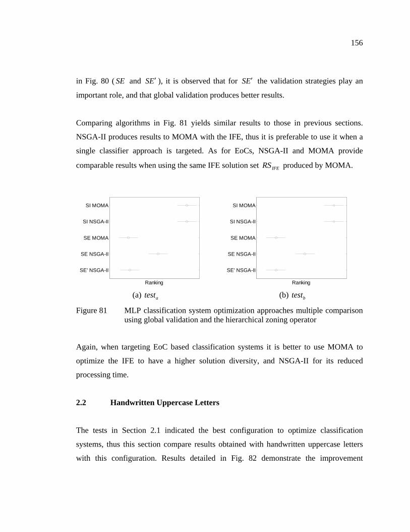
156
in Fig. 80 ( SE and ES ′ ), it is observed that for ES ′ the validation strategies play an
important role, and that global validation produces better results.
Comparing algorithms in Fig. 81 yields similar results to those in previous sections.
NSGA-II produces results to MOMA with the IFE, thus it is preferable to use it when a
single classifier approach is targeted. As for EoCs, NSGA-II and MOMA provide
comparable results when using the same IFE solution set IFERS produced by MOMA.
SE' NSGA-II
SE NSGA-II
SE MOMA
SI NSGA-II
SI MOMA
Ranking (a) atest
SE' NSGA-II
SE NSGA-II
SE MOMA
SI NSGA-II
SI MOMA
Ranking (b) btest
Figure 81 MLP classification system optimization approaches multiple comparison using global validation and the hierarchical zoning operator
Again, when targeting EoC based classification systems it is better to use MOMA to
optimize the IFE to have a higher solution diversity, and NSGA-II for its reduced
processing time.
2.2 Handwritten Uppercase Letters
The tests in Section 2.1 indicated the best configuration to optimize classification
systems, thus this section compare results obtained with handwritten uppercase letters
with this configuration. Results detailed in Fig. 82 demonstrate the improvement

157
SE
SI
Ranking (a)
SE
SI
Ranking (b)
Figure 82 Uppercase letters multiple comparison for PD (a) and MLP (b) classification system optimization, error rates measured on the test data set
obtained when optimizing an EoC SE in comparison to the best single classifier SI
selected. The tests confirmed that optimizing an EoC improves results with both
classifiers.

APPENDIX 3
Rejection strategies

159
Given an unknown observation x , a classifier tries to determine to which class iC the
observation x belongs to. The classification procedure calculates for each known class
iC the posterior probability ( )xCP i |ˆ , indicating the probability that x belongs to iC .
One strategy to reduce classification error is to reject observations that are likely to be
misclassified, so that they can be handled by more efficient means, such as human
verification.
Fumera proposed in [92] a method for classifier rejection using multiple thresholds
based on posterior probabilities. The MLP classifier outputs posterior probabilities for
each class, and the same applies to MLP EoCs. However, the PD classifier outputs
distances to hyper planes for each class iC , whereas the PD EoC outputs vote counts.
Thus, the first step to apply rejection is to have all classifiers outputs converted to
posterior probabilities for each class. This section first describes how the PD classifier
outputs (single classifier and EoC) are converted to posterior probabilities, describing
next Fumera’s method with multiple thresholds for rejection.
3.1 PD Classifier
The PD classifier outputs for each class a distance to a hyperplane. Thus, a rejection
strategy must first calculate the posterior probabilities to establish thresholds for
rejection. One commonly used function to create posterior probabilities for a classifier as
the PD is the softmax function. This neural transfer function converts the distance values
to values between 0 and 1 that sum up to 1.
For an unknown observation x , the distance ( )xdi to the hyper plane associated to class
iC (with n classes), the estimate of the posterior probability ( )xCP i |ˆ of x belonging to
class iC is calculated as in (3.1).

160
( )( )
( )∑=
= n
j
xd
xd
ij
i
e
exCP
1
|ˆ , (3.1)
Hensen’s method [104] is used to calculate posterior probabilities from PD EoC votes.
Given a PD EoC with N classifiers, the unknown observation x and ( )xiv | the vote
number for class iC , we have that the estimate of the posterior probability ( )xCP i |ˆ for
PD EoCs is calculated as
( ) ( )( )N
xxIvxCP i||ˆ = , (3.2)
where ( )xI is calculated as
( ) ( )xivxIn
j|maxarg
1== . (3.3)
3.2 Rejection With Multiple Thresholds
For a classification problem with n classes, the classifier will select the class iC the
observation x belongs to as the highest posterior probability ( )xCP i |ˆ . A traditional
single threshold rejection strategy [105] will reject observation x if
( ) ( ) TxCPxCP ij
n
j<=
=|ˆ|ˆmax
1, (3.4)
and it will accept observation x if

161
( ) ( ) TxCPxCP ij
n
j≥=
=|ˆ|ˆmax
1, (3.5)
where T is the threshold to decide if x is accepted or not after classification.
Fumera demonstrated in [92] that using class-related thresholds (CRT) yields higher
accuracies than using a single threshold T . With the CRT, observation x will be
rejected if
( ) ( ) iij
n
jTxCPxCP <=
=|ˆ|ˆmax
1, (3.6)
and it will be accepted if
( ) ( ) iij
n
jTxCPxCP ≥=
=|ˆ|ˆmax
1. (3.7)
An iterative process is used to calculate the threshold iT for each class iC , based on a
desired error rate e during the classification stage. This iterative process has to
systematically test different iT values until it finds a threshold that yields the desired
error rate e . This process is repeated for each class iC , until all thresholds are
calculated for the classification stage. As the error rate e is used to optimize all
thresholds, the overall classification error when all classes are combined is also e . This
statement is easily verified for any given data set D with n classes such as that
{ }nXXD ,,1 …= , where iX are the observations belonging to class iC . For an error rate
e , the number of misclassified observations mo is Demo = . This can be expanded to
( )nXXemo …+= 1 , which is equivalent to nXeXemo ++= …1 . This guarantees

162
that searching for each threshold iT independently with a fixed error rate e will yield an
overall error rate e for the complete data set D .
Algorithm Algorithm 12 details an algorithm version of the iterative process, calculating
the threshold iT for the observation set iX belonging to all classes iC . The process
requires a threshold increment a to systematically test threshold values. a should be a
small value to allow a more accurate calculation to the threshold iT . The algorithm starts
with the threshold 0=iT , accepting all ( )xCP i |ˆ . It then increments its value until it
achieves the desired error rate e and stopping the procedure.
Algorithm 12: Algorithm used to calculate the rejection thresholds given the desired error rate e Data: desired error rate e , threshold increment a , data set D Result : The thresholds nTT ,,1 …
0, =∈∀ idFi ; for 1=i to n do 0=iT ; repeat
aTT ii += ;
Calculate error , the classification error rate of iX using the
threshold iT ;
until eerror ≥ ; end
During the classification stage, observations are rejected according to (3.6) or accepted
if (3.7) is true. This procedure was used in Chapters 6 and 7 to create error-rejection
curves and evaluate classifier accuracy with fixed error rates.

BIBLIOGRAPHY
[1] J. H. Holland, Adaptation in Natural and Artificial Systems. MIT Press, 1975. [2] C. M. Bishop, Neural Networks for Pattern Recognition. Oxford University Press,
1995 [3] C. Cortes and V. Vapnik, “Support-vector networks”, Machine Learning, vol. 20,
no. 3, pp. 273–297, 1995. [4] C. J. C. Burges, “A tutorial on support vector machines for pattern recognition”,
Data Mining and Knowledge Discovery, vol. 2, no. 2, pp. 121–167, 1998. [5] T. G. Dietterich, “Ensemble Learning”, in The Handbook of Brain Theory and
Neural Networks, 2nd ed., M. A. Arbib, Ed. MIT Press, 2002. [6] J. Kittler, M. Hatef, R. P. W. Duin, and J. Matas, “On combining classifiers”,
IEEE Transactions on Pattern Analysis and Machine Intelligence, vol. 20, no. 3, pp. 226–239, 1998.
[7] A. Lemieux, C. Gagné, and M. Parizeau, “Genetical Engineering of Handwriting
Representation”, in Proceedings of the Eigth International Workshop on Frontiers in Handwriting Recognition – IWFHR-8. Ontario, Canada: IEEE Computer Society, 2002, pp. 145–150.
[8] A. Teredesai, J. Park, and V. Govindaraju, “Active Handwritten Character
Recognition using Genetic Programming”, in Proceedings of the European Conference on Genetic Programming – EuroGP, 2001, pp. 371–380.
[9] C. Emmanouilidis, A. Hunter, and J. MacIntyre, “A multiobjective evolutionary
setting for feature selection and a commonality-based crossover operator”, in Proceedings of the 2000 Congress on Evolutionary Computation – CEC00, California, USA, IEEE Press, 2000, pp. 309–316.
[10] L. S. Oliveira, R. Sabourin, F. Bortolozzi, and C. Y. Suen, “A Methodology for
Feature Selection Using Multi-Objective Genetic Algorithms for Handwritten DigitString Recognition”, International Journal of Pattern Recognition and Artificial Intelligence, vol. 17, no. 6, pp. 903–929, 2003.
[11] D. Ruta and B. Gabrys, “Classifier Selection for Majority Voting”, Information
Fusion, vol. 6, pp. 63–81, 2005.

164
[12] L. I. Kuncheva and L. C. Jain, “Design classifier fusion systems by genetic algorithms”, IEEE Transactions on Evolutionary Computation, vol. 4, no. 4, pp. 327–336, 2000.
[13] G. Tremblay, R. Sabourin, and P. Maupin, “Optimizing nearest neighbour in
random subspaces using a multi-objective genetic algorithm”, in 17th International Conference on Pattern Recognition – ICPR2004, Cambridge, U.K.: IEEE Computer Society, August 2004, pp. 208–211.
[14] S. D. Bay, “Combining nearest neighbor classifiers through multiple feature
subsets”, in Proc. 15th International Conf. on Machine Learning, Morgan Kaufmann, San Francisco, CA, 1998, pp. 37–45.
[15] T. K. Ho, “Nearest neighbors in random subspaces”, in Proceedings of the 2nd Int'l
Workshop on Statistical Techniques in Pattern Recognition, Sydney, Australia, August 1998, pp. 640–648.
[16] P. J. Grother, NIST Special Database 19 – Handprinted forms and characters
database, National Institute of Standards and Technoloy NIST, 1995, database, CD documentation.
[17] P. V. W. Radtke, L. S. Oliveira, R. Sabourin, and T. Wong, “Intelligent Zoning
Design Using Multi-Objective Evolutionary Algorithms”, in Proceedings of the 7th International Conference on Document Analysis and Recognition – ICDAR2003. Edinburg, Scotland: IEEE Computer Society, August 2003, pp. 824–828.
[18] P. V.W. Radtke, T.Wong, and R. Sabourin, “A Multi-Objective Memetic
Algorithm for Intelligent Feature Extraction”, in Proceedings of the Third International Conference on Evolutionary Multi-Criterion Optimization – EMO 2005. Berlin: Springer-Verlag, 2005, pp. 767–781.
[19] P. V. W. Radtke, R. Sabourin, and T. Wong, “Intelligent feature extraction for
ensemble of classifiers”, in Proceedings of the 8th International Conference on Document Analysis and Recognition – ICDAR 2005. IEEE Computer Society, 2005, pp. 866–870.
[20] P. V. W. Radtke, T. Wong, and R. Sabourin, “Classification system optimization
with multi-objective genetic algorithms”, in Proceedings of the 10th International Workshop on Frontiers in Handwriten Recognition – IWFHR 2006. IAPR, 2006, in press.

165
[21] P. V. W. Radtke, T. Wong, and R. Sabourin, “An evaluation of over-fit control strategies for multi-objective evolutionary optimization”, in Proceedings of the International Joint Conference on Neural Networks – IJCNN 2006.IEEE Computer Society, 6359–6366, 2006.
[22] Øivind Dur Trier, A. K. Jain, and T. Taxt, “Feature Extraction Methods for
Character Recognition – A Survey”, Pattern Recognition, vol. 29, no. 4, pp. 641–662, 1996.
[23] R. R. Bailey and M. Srinath, “Orthogonal Moment Features for use with
Parametric and Non-Parametric Classifiers”, IEEE Transactions on Pattern Analysis and Machine Intelligence, vol. 18, no. 4, pp. 389–399, 1996.
[24] P. D. Gader, “Automatic Feature Generation for Handwritten Digit Recognition”,
IEEE Transactions on Pattern Analysis and Machine Intelligence, vol. 18, no. 12, pp. 1256–1261, 1996.
[25] I.-S. Oh and C. Y. Suen, “Distance features for neural network-based recognition
of handwritten characters”, International Journal on Document Analysis and Recognition, vol. 2, no. 1, pp. 873–885, 1998.
[26] L. Heutte, T. Paquet, J. Moreau, Y. Lecourtier, and C. Olivier, “A
structural/statistical feature based vector for handwritten character recognition”, Pattern Recognition Letters, vol. 19, no. 7, pp. 629–641, 1998.
[27] V. di Lecce, G. Dimauro, A. Guerriero, S. Impedovo, G. Pirlo, and A. Salzo,
“Zoning Design for Hand-Written Numeral Recognition”, in Proceedings of the Seventh International workshop on Frontiers in Handwriting Recognition – IWFHR-7, 2000, pp. 583–588.
[28] R. Sabourin, M. Cheriet, and G. Genest, “An Extended-Shadow-Code Based
Approach for Off-Line Signature Verification”, in Proceedings of The Second IAPR Conf. on Document Analysis and Recognition, Tsukuba, Japan, 1993, pp. 1–5.
[29] R. Sabourin, G. Genest, and F. J. Prêteux, “Off-line signature verification by local
granulometric size distributions”, IEEE Transactions on Pattern Analysis and Machine Intelligence, vol. 19, no. 9, pp. 976–988, 1997.
[30] L. S. Oliveira, R. Sabourin, F. Bortolozzi, and C. Y. Suen, “Feature Selection
Using Multi-Objective Genetic Algorithms for Handwritten Digit Recognition”, in Proceedings of the 16th IAPR International Conference on Pattern Recognition. IEEE Computer Society, 2002, pp. 568–571.

166
[31] G. F. Houle, D. B. Aragon, R. W. Smith, M. Shridhar, and D. Kimura, “Multi-Layered Corroboration-Based Check Reader”, in Proceedings of The International Association for Pattern Recognition Workshop on Document Analysis Systems – DAS'96, 1996, pp. 495–546.
[32] Z.-C. Li and C. Y. Suen, “The partition-combination method for recognition of
handwritten characters”, Pattern Recognition Letters, vol. 21, no. 8, pp. 701–720, 2000.
[33] A. L. Koerich, “Large Vocabulary Off-Line HandwrittenWord Recognition”,
Ph.D. dissertation, École de Technologie Supérieure – ETS – Université du Québec, Montreal, Québec, Canada, 2002.
[34] C.-L. Liu, H. Sako, and H. Fujisawa, “Performance evaluation of pattern
classifiers for handwritten character recognition”, International Journal on Document Analysis and Recognition, vol. 3, no. 4, pp. 191–204, 2002.
[35] M. Kudo and J. Sklansky, “Comparison of algorithms that select features for
pattern classifiers”, Pattern Recognition, vol. 33, no. 1, pp. 25–41, 2000. [36] A. W. Whitney, “A Direct Method of Non-Parametric Measurement Selection,
IEEE Transactions on Computers, vol. 20, no. 9, pp. 1100–1103, 1971. [37] P. Pudil, J. Novovicova;, and J. Kittler, “Floating search methods in feature
selection”, Pattern Recogn. Letters, vol. 15, no. 11, pp. 1119–1125, 1994. [38] P. Narendra and K. Fukunaga, “A branch and bound algorithm for feature subset
selection”, IEEE Transactions on Computers, vol. 26, no. 9, pp. 1917–1922, 1977. [39] D. E. Goldberg, Genetic Algorithms in Search, Optimization and Machine
Learning. New York, NY, USA: Addison Wesley, 1989. [40] H. Yuan, S.-S. Tseng,W. Gangshan, and Z. Fuyan, “A Two-phase Feature
Selection Method using both Filter and Wrapper”, in Proceedings of the IEEE International Conference on Systems, Man and Cybernetics – SMC'99, vol. 2, 1999, pp. 132–136.
[41] L. Breiman, “Bagging predictors”, Machine Learning, vol. 24, no. 2, pp. 123–140,
1996.
[42] R. Schapire, The boosting approach to machine learning: An overview, 2001. [Online]. Available: http://www.research.att.com/ schapire/boost.html

167
[43] L. S. Oliveira, R. Sabourin, F. Bortolozzi, and C. Y. Suen, “A methodology for feature selection using multi-objective genetic algorithms for handwritten digit string recognition”, International Journal of Pattern Recognition and Artificial Intelligence – IJPRAI, vol. 17, no. 6, pp. 903–929, 2003.
[44] L. S. Oliveira, M. Morita, R. Sabourin, and F. Bortolozzi, “Multi-Objective
Genetic Algorithms to Create Ensemble of Classifiers”, in Proceedings of the Third International Conference on Evolutionary Multi-Criterion Optimization – EMO 2005. Berlin: Springer-Verlag, 2005, pp. 592–606.
[45] L. S. Oliveira, R. Sabourin, F. Bortolozzi, and C. Y. Suen, “Feature selection for
ensembles : A hierarchical multi-objective genetic algorithm approach”, in Proceedings of the 7th International Conference on Document Analysis and Recognition – ICDAR2003, Edinburg, Scotland, August 2003, pp. 676–680.
[46] J. Reunanen, “Overfitting in making comparisons between variable selection
methods”, Journal of Machine Learning Research, no. 3, pp. 1371–1382, 2003. [47] J. Loughrey and P. Cunningham, “Overfitting in wrapper-based feature subset
selection: The harder you try the worse it gets”, in Proceedings of International Conference on Innovative Techniques and Applications of Artificial Intelligence, 2004, pp. 33–43.
[48] J. Loughrey and P. Cunningham , “Using early-stopping to avoid overfitting in
wrapper-based feature subset selection employing stochastic search”, Department of Computer Science, Trinity College, Tech. Rep. TCD-CS-2005-37, 2005.
[49] X. Llorà, D. Goldberg, I. Traus, and E. B. i Mansilla, “Accuracy, parsimony, and
generality in evolutionary learning systems via multiobjective selection”, in International Workshop in Learning Classifier Systems, 2002, pp. 118–142.
[50] E. B. i Mansilla, X. Llorà, and I. Traus, “Multiobjective learning classifier
systems”, Studies in Computational Intelligence, vol. 16, pp. 261–288, 2006. [51] L. S. Oliveira, R. Sabourin, F. Bortolozzi, and C. Y. Suen, “Automatic
Recognition of Handwritten Numerical Strings: A Recognition and Verification Strategy”, IEEE Trans. on Pattern Analysis and Machine Intelligence, vol. 24, no. 11, pp. 1438–1454, 2002.
[52] S. Bandyopadhyay, S. K. Pal, and B. Aruna, “Multiobjective GAs, Quantitative Indices, and Pattern Classification”, IEEE Transactions on System, Man, and Cybernetics – Part B: Cybernetics, vol. 34, no. 5, pp. 2088–2099, 2004.

168
[53] K. Deb, Multi-Objective Optimization using Evolutionary Algorithms. Baffins Lane, Chichester, West Sussex, PO19 1UD ,England: John Wiley & Sons, LTD, 2001.
[54] J. D. Schaffer, “Multiple objective optimization with vector evaluated genetic
algorithms”, in Proceedings of the First International Conference on Genetic Algorithms – ICGA, J. J. Grefenstette, Ed. Lawrence Erlbaum Associates, 1985, pp. 93–100.
[55] C. A. C. Coello, “Evolutionary multi-objective optimization: a historical view of
the field”, IEEE Computational Intelligence Magazine, vol. 1, no. 1, pp. 28–36, 2006.
[56] N. Srinivas and K. Deb, “Multiobjective optimization using nondominated sorting
in genetic algorithms”, Evolutionary Computation, vol. 2, no. 3, pp. 221–248, 1994.
[57] K. Deb and T. Goel, “Controlled elitist non-dominated sorting genetic algorithms
for better convergence”, in Proceedings of the First International Conference on Evolutionary Multi-Criterion Optimization – EMO 2001, E. Zitzler, K. Deb, L. Thiele, C. A. C. Coello, and D. Corne, Eds. Berlin: Springer-Verlag, 2001, pp. 67–81.
[58] E. Zitzler, M. Laumanns, and L. Thiele, “SPEA2: Improving the strength pareto
evolutionary algorithm for multiobjective optimization”, in Evolutionary Methods for Design Optimization and Control with Applications to Industrial Problems, K. C. Giannakoglou, D. T. Tsahalis, J. PÈriaux, K. D. Papailiou, and T. Fogarty, Eds. Athens, Greece: International Center for Numerical Methods in Engineering – Cmine, 2001, pp. 95–100.
[59] W. M. Spears, The role of mutation and recombination in evolutionary algorithms,
Ph.D. dissertation, George Mason University, Fairfax, Virginia, USA, 1998. [60] H. Ishibuchi and K. Narukawa, “Recombination of Similar Parents in EMO
Algorithms”, in Proceedings of the Third International Conference on Evolutionary Multi-Criterion Optimization – EMO 2005. Berlin: Springer-Verlag, 2005, pp. 265–279.
[61] D. A. V. Veldhuizen and G. B. Lamont, “Multiobjective Evolutionary Algorithms:
Analyzing the State-of-the-Art”, IEEE Transactions on Evolutionary Computation, vol. 2, no. 8, pp. 125–147, 2000.

169
[62] E. Zitzler, K. Deb, and L. Thiele, “Comparison of Multiobjective Evolutionary Algorithms: Empirical Results”, Evolutionary Computation Journal, vol. 2, no. 8, pp. 125–148, 2000.
[63] K. Deb, S. Agrawal, A. Pratab, and T. Meyarivan, “A Fast Elitist Non-Dominated
Sorting Genetic Algorithm for Multi-Objective Optimization: NSGA-II”, in Proceedings of the Parallel Problem Solving from Nature VI Conference, Paris, France, 2000, pp. 849–858.
[64] E. Cantú-Paz, Efficient and Accurate Parallel Genetic Algorithms. Norwell,
Massachussets 02061 USA: Kluwer Academic Publishers, 2000. [65] Dubreuil, M., Gagné, C., Parizeau, M., “Analysis of a Master-Slave Architecture
for Distributed Evolutionary Computations”, IEEE Transactions on Systems, Man and Cybernetics, vol. 36, no. 1, pp. 229–235, 2006.
[66] E. Cantú-Paz, “A survey of parallel genetic algorithms”, Calculateurs Paralleles,
Reseaux et Systems Repartis, vol. 10, no. 2, pp. 141–171, 1998. [67] T. Hiroyasu, M. Miki, and M. Masaki, “A new model of distributed genetic
algorithm for cluster systems: Dual individual DGA”, in Proceedings of High Performance Computing Conference - Lecture Notes in Computer Science 1940. Springer Verlag, 2000, pp. 374–383.
[68] T. Hiroyasu, M. Miki, and S. Watanabe, “Divided Range Genetic Algorithms in
Multiobjective Optimization Problems”, in Proceedings of the International Workshop on Emergent Synthesis – IWES'99, 1999, pp. 57–66.
[69] Z.-Y. Zhu and K.-S. Leung, “Asynchronous Self-Adjustable Island Genetic
Algorithm for Multi-Objective Optimization Problems”, in Proceedings of the Congress on Evolutionary Computation. IEEE, 2002, pp. 837–842.
[70] F. Streichert, H. Ulmer, and A. Zell, “Parallelization of multi-objective
evolutionary algorithms using clustering algorithms”, in Proceedings of the Third International Conference on Evolutionary Multi-Criterion Optimization – EMO 2005. Berlin: Springer-Verlag, 2005, pp. 92–107.
[71] J. Knowles, “On Metrics for Comparing nondominated Sets”, in Proceedings of
the 2002 Conference on Evolutionary Computation – CEC'2002. Honolulu, Hawaii, USA: IEEE, 2002, pp. 711–716.

170
[72] E. Zitzler, L. Thiele, M. Laumanns, C. M. Fonseca, and V. G. Fonseca, “Performance Assesment of Multiobjective Optimizers: An Analysis and Review”, IEEE Transactions on Evolutionary Computation, vol. 7, no. 2, pp. 117–132, 2003.
[73] E. Zitzler, Evolutionary algorithms for multiobjective optimization: Methods and
applications, Ph.D. dissertation, Swiss Federal Institute of Technology Zurich, 1999.
[74] E. Zitzler and L. Thiele, “Multiobjective Optimization Using Evolutionary
Algorithms – A Comparative Case Study”, in Parallel Problem Solving from Nature – PPSVN V. Springer Verlag, 1998, pp. 292–301.
[75] L. Heutte, J. Moreau, B. Plessis, J. Plagmaud, and Y. Lecourtier, Handwritten
numeral recognition based on multiple feature extractors”, in Proceedingss of 2nd ICDAR, 1993, pp. 167–170.
[76] G. Dimauro, S. Impedovo, G. Pirlo, and A. Salzo, “Zoning design for handwritten
numeral recognition”, in ICIA (2), 1997, pp. 592–599. [77] G. H. John, R. Kohavi, and K. Pfleger, “Irrelevant features and the subset selection
problem”, in International Conference on Machine Learning, 1994, pp. 121–129. [78] K. Chen and H. Liu, “Towards an evolutionary algorithm: A comparison of two
feature selection algorithms”, in 1999 Congress on Evolutionary Computation, 1999, pp. 1309–1313.
[79] F. Kimura, S. Inoue, T. Wakabayashi, S. Tsuruoka, and Y. Miyake, “Handwritten
Numeral Recognition using Autoassociative Neural Networks”, in Proceedings of the International Conference on Pattern Recognition, 1998, pp. 152–155.
[80] A. El-Yacoubi, M. Gilloux, R. Sabourin, and C. Y. Suen, “Objective Evaluation of
the Discriminant Power of Features in an HMM-basedWord Recognition System”, in Proceedings of the 1997 Brazilian Symposium on Documents and Image Analysis – BSDIA'97, Curitiba, PR, Brazil, 1997, pp. 60–73.
[81] L. S. Oliveira, N. Benahmed, R. Sabourin, F. Bortolozzi, and C. Y. Suen, “Feature
subset selection using genetic algorithms for handwritten digit recognition”, in Proceedings of the 14th Brazilian Symposium on Computer Graphics and Image Processing. Florianópolis-Brazil: IEEE Computer Society, 2001, pp. 362–369.

171
[82] J. Moody and J. Utans, “Principled architecture selection for neural networks: Application to corporate bond ratings predictions”, in Advances in Neural Information Processing Systems, J. Moody, S. Hanson, and R. P. Lippman, Eds. Morgan Kauffman, 2001, vol. 4, pp. 683–690.
[83] T. Murata, H. Nozawa, Y. Tsujimura, M. Gen, and H. Ishibuchi, “Effect of Local
Search on the Performance of Cellular Multi-Objective Genetic Algorithms for Designing Fuzzy Rule-based Classification Systems”, in Proceedings of the 2002 Conference on Evolutionary Computation - CEC'2002, 2002, pp. 663–668.
[84] H. Ishibuchi, T. Yoshida, and T. Murata, “Balance Between Genetic Search and
Local Search in Memetic Algorithms for Multiobjective Permutation Flowshop Scheduling”, IEEE Transactions on Evolutionary Computation, vol. 7, no. 2, pp. 204–223, 2003.
[85] J. D. Knowles and D. Corne, “Memetic algorithms for multiobjective
optimization: issues, methods and prospects”, in Recent Advances in Memetic Algorithms. Springer Verlag, 2004, pp. 313–352.
[86] N. Krasnogor and J. Smith, “A tutorial for competent memetic algorithms: Model,
taxonomy, and design issues”, IEEE Transactions on Evolutionary Computation, vol. 9, no. 5, pp. 474–488, 2005.
[87] A. Jaszkiewicz, “Do Multiple-Objective Metaheuristics Deliver on Their Promise?
A Computational Experiment on the Set-Covering Problem”, IEEE Transactions on Evolutionary Computation, vol. 7, no. 2, pp. 133–143, 2003.
[88] G. Parks, L. Jianping, M. Balazs, and I. Miller, “An Empirical Investigation of
Elitism in Multiobjective Genetic Algorithms”, Foundations of Computing and Decision Sciences, vol. 26, no. 1, pp. 51–74, 2001.
[89] J. W. Pepper, B. L. Golden, and E. A. Wasil, “Solving the traveling salesman
problem with annealing-based heuristics: A computationa study”, IEEE Trans. On Systems, Mand and Cybernetics – Part A: Systems and Humans, vol. 32, no. 1, pp. 72–77, 2002.
[90] Ágoston Endre Eiben, R. Hinterdind, and Z. Michalewicz, “Parameter control in
evolutionary algorithms”, IEEE Transactions on Evolutionary Computation, vol. 3, no. 2, pp. 124–141, 1999.
[91] R. F. Gunst and R. L. Mason, How to Construct Fractional Factorial Experiments
– ASQC basic references on quality control: v. 14. 611 East Wisconsin Avenue, Milwaukee, Wisconsin 53202, USA: American Society for Quality Control – Statistics Division, 1991.

172
[92] G. Fumera, F. Roli, and G. Giacinto, “Reject option with multiple thresholds”,
Pattern Recoginition, vol. 33, no. 12, pp. 2099–2101, 2000. [93] J. Milgram, R. Sabourin, and M. Cheriet, “Estimating posterior probabilities with
support vector machines: A case study on isolated handwritten character recognition”, submitted to the IEEE Transactions on Neural Networks, 2006.
[94] S. E. N. Correia, Reconhecimento de caracteres manuscritos usando wavelets,
Master dissertation, Campina Grande, Paraíba, Brazil, 2005. [95] C.-L. Liu and H. Sako, “Class-specific feature polynomial classifier for pattern
classification and its application to handwritten numeral recognition”, Pattern Recognition, vol. 39, no. 4, pp. 669–681, 2006.
[96] G. L. Pappa, A. A. Freitas, and C. A. A. Kaestner, “Multi-objective algorithms for
attribute selection in data mining”, in Applications of Multi-Objective Evolutionary Algorithms, C. C. Coello and G. Lamont, Eds. World Scientific, December 2004, pp. 603–626.
[97] F. Schlotmann, A. Mitschele, and D. Seese, “A Multi-Objective Approach to
Integrated Risk Management”, in Proceedings of the Third International Conference on Evolutionary Multi-Criterion Optimization – EMO 2005. Berlin: Springer-Verlag, 2005, pp. 692–706.
[98] B. de la Iglesia, A. Reynolds, and V. J. Rayward-Smith, “Developments on a
Multi-objective Metaheuristic (MOMH) Algorithm for Finding Interesting Sets of Classification Rules”, in Proceedings of the Third International Conference on Evolutionary Multi-Criterion Optimization – EMO 2005. Berlin: Springer-Verlag, 2005, pp. 826–840.
[99] R. O. Day and G. B. Lamont, “Extended Multi-objective fast messy Genetic
Algorithm Solving Deception Problems”, in Proceedings of the Third International Conference on Evolutionary Multi-Criterion Optimization – EMO 2005. Berlin: Springer-Verlag, 2005, pp. 296–310.
[100] L. Jourdan, D. Corne, D. Savic, and G. Walters, “Preliminary Investigation of the
‘Learnale Evolution Model’ for Faster/Better Multiobjective Water Systems Design”, in Proceedings of the Third International Conference on Evolutionary Multi-Criterion Optimization – EMO 2005. Berlin: Springer-Verlag, 2005, pp. 841–855.

173
[101] Y. Nojima, K. Narukawa, S. Kaige, and H. Ishibuchi, “Effects of Removing Overlapping Solutions on the Performance of the NSGA-II Algorithm”, in Proceedings of the Third International Conference on Evolutionary Multi-Criterion Optimization – EMO 2005. Berlin: Springer-Verlag, 2005, pp. 341–354.
[102] J. B. Kollat and P. M. Reed, “The Value of Online Adaptative Search: A
Performance Comparison of NSGA-II, ε-NSGA-II and ε-MOEA”, in Proceedings of the Third International Conference on Evolutionary Multi-Criterion Optimization – EMO 2005. Berlin: Springer-Verlag, 2005, pp. 386–398.
[103] D. Greiner, G. Winter, J. M. Emperador, and B. Galván, “Gray Coding in
Evolutionary Multicriteria optimization: Application in Frame Structural Optimum Design”, in Proceedings of the Third International Conference on Evolutionary Multi-Criterion Optimization – EMO 2005. Berlin: Springer-Verlag, 2005, pp. 576–591.
[104] L. K. Hensen, C. Liisberg, and P. Salamon, “The error-reject tradeoff”, Open
Systems & Information Dynamics, vol. 4, no. 2, pp. 159–184, 1997. [105] C. K. Chow, “On optimium error and reject tradeoff”, IEEE Transactions on
Information Theory, vol. 16, no. 1, pp. 41–46, 1970.
