ecommerce and market structure effects in the european ...741142/fulltext01.pdf · ecommerce and...
TRANSCRIPT

Ecommerce and market structure effects in the European retail industry
FREDRIK WERNER
Master of Science Thesis
Stockholm, Sweden 2012

Ecommerce and market structure effects in the European retail industry
Fredrik Werner
Master of Science Thesis INDEK 2012:106
KTH Industrial Engineering and Management
SE-100 44 STOCKHOLM

Fredrik Werner
3
Master of Science Thesis INDEK 2012:106
Ecommerce and market structure effects in the European retail industry
{Fredrik Werner}
Approved
2012-08-14
Examiner
Kristina Nyström
Supervisor
Marcus Asplund
Abstract Fifteen or so years into what is said to be the game changer of our time there are many fields of
science focusing their attention towards the online market in attempts to describe its
implications for the traditional, offline markets. Where most of the literature on economics of
ecommerce focus on pricing mechanisms and growth little attention has been directed towards
more general market structure effects. This thesis adopts techniques, empirical and theoretical
models from the search cost and market structure literature in order to examine the
relationships between ecommerce and offline market structures in the retail industry through
regional employment and establishment data. The literature reviewed and used focus only on
the US market whereas this thesis shifts the attention to the European regions. The results are
convincing and in general corresponding to previous research results. As ecommerce usage
increase and the consumer search costs thereby gets lower inefficient firms drop out of the
market resulting in a decline in local establishment counts. The opposite effect is seen for pure
online retailing establishments that thrive in the presence of local ecommerce usage. The effect
of ecommerce on traditional offline establishments seems to be aggregated phenomena
whereas the effect on pure online firms seems to be of a more local nature. Focus of
policymakers and company management therefore might consider looking at the two effects in
their respective aggregation level to best sort out how to react in the presence of increased
competition from ecommerce usage.
Ecommerce, Market structure, Regional analysis, European retail industry, Panel
data, Fixed effects modeling
Fredrik Werner
4
Contents
Introduction .................................................................................................................................. 6
E-commerce .............................................................................................................................. 6
Market figures and trends ...................................................................................................... 7
Purpose of the study .................................................................................................................. 10
Scope ......................................................................................................................................... 10
Method ..................................................................................................................................... 10
Limitations .............................................................................................................................. 10
Literature review and theoretical background ................................................................... 11
Ecommerce and Prices .......................................................................................................... 11
Ecommerce and information Asymmetry ......................................................................... 12
Ecommerce and Search Costs .............................................................................................. 12
Ecommerce and geography .................................................................................................. 14
Firm survival and exit ........................................................................................................... 15
Market effects ......................................................................................................................... 16
Research question and Hypothesis ........................................................................................ 16
Causation and Correlation ....................................................................................................... 17
Data description ......................................................................................................................... 18
Eurostat Dataset ................................................................................................................. 18
Industry definition............................................................................................................. 18
Market Definition ............................................................................................................... 19
Time period ......................................................................................................................... 20
Variables description ........................................................................................................ 20
Descriptive statistics ......................................................................................................... 22
Data figures ......................................................................................................................... 23
Data quality ......................................................................................................................... 24
Empirical models and econometric method......................................................................... 25
Empirical models ................................................................................................................... 25

Fredrik Werner
5
Model 1a ............................................................................................................................... 25
Model 1b ............................................................................................................................... 26
Model 2 ................................................................................................................................. 26
Model 3 ................................................................................................................................. 27
Model 4 ................................................................................................................................. 27
Econometric method ............................................................................................................. 27
Fixed vs. random effects model ....................................................................................... 28
Econometric model specification ................................................................................... 28
Econometric model specification problems ................................................................. 30
Unit root testing and non-stationarity ........................................................................... 30
Econometric variables and model specifications ........................................................ 31
Expected coefficients ......................................................................................................... 34
Results and tables ...................................................................................................................... 35
Result analysis ............................................................................................................................ 37
General ..................................................................................................................................... 37
Model 1 ..................................................................................................................................... 38
Model 2 ..................................................................................................................................... 38
Model 3 ..................................................................................................................................... 39
Model 4 .................................................................................................................................... 39
Comments and conclusion ....................................................................................................... 40
Further research ........................................................................................................................ 41
REFERECES .................................................................................................................................. 42
APPENDIX .................................................................................................................................... 44

Fredrik Werner
6
Introduction
This paper will look into previous work on e-commerce diffusion and its effects on the structure
of the retail industry. Empirical analyses are carried out on regional effects in a sample of
European regions. The empirical models will be based on previous empirical and theoretical
work that most often only have focused their attention on the US markets. With this thesis I
seek to examine how well the predictions in previous models and the findings of previous
empirical analyses hold in the European context1. One of the main reasons to carry out these
empirical tests of already “verified” models is due to the fact that US ecommerce has
established and diffused throughout the country at a much higher rate than it has in rest of the
world. When the European countries now start to adopt ecommerce at a higher rate they build
their growth on already made errors and on a market where knowledge about possible effects
are known. Therefore the possibility that the market structure effects will differ from the early
adopters in the US is always present. For firms building their strategies in the European market
context this it is important to know both the similarities and the differences between the two
markets.
Before turning to previous findings and models we will lay out some facts about ecommerce as
such and also show recent trends and market figures.
E-commerce Fifteen or so years into what is said to be the game changer of our time there are many fields of
science focusing their attention towards the online market to describe its implications for the
traditional, offline markets. This section will enlighten some of the recent trends and facts about
the online market and the different actors in it. A general description of the current worldwide
trends and figures will be followed by a description of Sweden in particular. Since the main focus
of this thesis is to untangle the effects that ecommerce has on the structure and competition in
the traditional retail markets, comparisons are made when necessary with facts from the offline
equivalent.
Before we go any further a clarification about what ecommerce is, in the context of this paper,
might be in order. For quite some time firms of different sort and size have used the internet to
conduct transactions of information, order goods and services from each other and make
payments. In the typical industrialized market the so called B2B (business to business)
ecommerce activities outweigh the B2C (business to consumer) ecommerce by far. This balance
however is changing rapidly and much of the attention made by researchers is focused on the
latter, B2C, ecommerce. This paper will do the same, leaving the interchange between firms that
often take place out of reach from the outside world to itself. Ecommerce can be broadly
described as “…conducting transactions along the value chain by using the Internet platform”
(Zhu, et al: 2006). In other words, think of e-commerce as an online marketplace where anyone
can go and buy what they need, both consumers and other firms. The big difference from a
1 ‘EU’ in this thesis includes regions from within the EU27 member nations and also neighboring European
countries such as Switzerland and Norway.
Fredrik Werner
7
regular marketplace is that this one has no opening hours and is simultaneously located
everywhere. The value for an existing or new firm in using ecommerce therefore lays in the
increased efficiency when penetrating new markets, reaching more people, becoming more
efficient in sales, using less inventory, having higher financial returns on sales etc. (Oliviera,
Martins; 2010). The reason why there might be increased efficiency in this is of course due to
the nature of the internet as a global information network which any player with the right
knowledge and infrastructure can use at any time.
The growth rate of ecommerce has been staggering. The latest figures suggest that the overall
market in Europe grew by 14% 2011. (DIBS; 2011) Taking into consideration that the market has
been growing at similar rates for more than a decade this is a significant rate. Even though
ecommerce only makes a small share of the total consumption in retail markets they act as a
powerful market force with price setting and structure changing abilities. On an international
level, not surprisingly, the ecommerce adoption and diffusion has varied quit much. Even within
the European Union the rate of which ecommerce is used by sellers (firms) and buyers
(indiviuals) differ much more than the trade taking place on offline markets. (nVision, 2008) The
most basic of necessities for the online market to evolve in a country is of course access to the
internet but also readily available financial intermediaries and a well-functioning transport
sector. These are factors that differ more between the EU nations than for example other large
economic areas such as the US. (nVision, 2008) On the other hand we move towards a more and
more homogenized market in the EU with free-trade agreements in place for several decades.
What still makes up the biggest barriers for ecommerce diffusion is payment methods. This is
according to a report by DIBS (2011) the single most differentiating market structure component
between regions in the EU as it affects the relative competitive advantage of online and offline
retailers in the region.
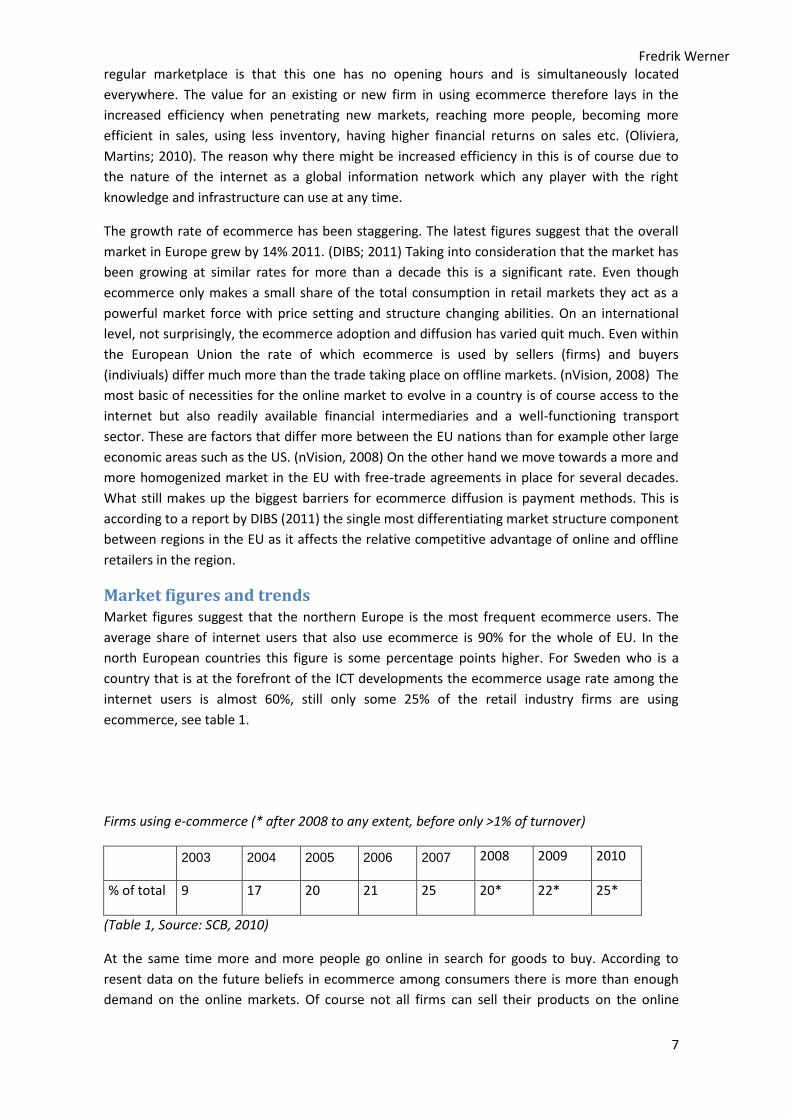
Market figures and trends Market figures suggest that the northern Europe is the most frequent ecommerce users. The
average share of internet users that also use ecommerce is 90% for the whole of EU. In the
north European countries this figure is some percentage points higher. For Sweden who is a
country that is at the forefront of the ICT developments the ecommerce usage rate among the
internet users is almost 60%, still only some 25% of the retail industry firms are using
ecommerce, see table 1.
Firms using e-commerce (* after 2008 to any extent, before only >1% of turnover)
2003 2004 2005 2006 2007 2008 2009 2010
% of total 9 17 20 21 25 20* 22* 25*
(Table 1, Source: SCB, 2010)
At the same time more and more people go online in search for goods to buy. According to
resent data on the future beliefs in ecommerce among consumers there is more than enough
demand on the online markets. Of course not all firms can sell their products on the online

Fredrik Werner
8
markets. Some goods might be too difficult to transport or just be of such character that it
would be impossible to sell online (e.g. a cup of coffee). Looking at the general trend for the
entire European region we see growth in ecommerce usage both by firms and consumers. This
however is not the same as to say that all countries and regions are using ecommerce equally
much. One of the foremost reasons of course being the availability of internet but also the
nature of ecommerce firms ability to cross boarders and reach consumers in other countries or
regions. A topic later discussed in this thesis is the local growth in ecommerce and how this
effects the local business environment, which would shed some more light on which process is
the most important; the local ecommerce growth or the surrounding regions ecommerce
growth.
It is reasonable to argue that the effect of online purchases would strike throughout the
internet-active population and probably effect businesses that has a further distance to its
customers harder than more close to market businesses. Ecommerce activity measures suggest
that the distance to consumer or agglomerated/ non agglomerated area effect differs quite a bit
between countries in Europe. Figure 2 below showcase this difference in patterns between two
countries that in terms of ICT readiness (access to internet and computer technology among the
population) are very much the same. There seems to be an effect of local market competition,
as will be presented further in the literature section, which is more relevant than the
geographical and ICT settings in explaining ecommerce usage patterns. The competitive settings
of the local market in this context is any market force that drives the customer to search for the
lowest possible price on a good or that makes firms compete in prices or quality at a relatively
higher rate than in less competitive markets.
Figure 2, Differences in ecommerce activity patterns
(Source; DIBS 2011)
These competitive forces are very much linked to the possible effects of increased ecommerce
activity and many of the early ecommerce economics papers published prior to the ICT bubble
burst in 2001 spoke about “revolutions” in the way market competition would take place and
how the firm 2.0 would look like before long. Even though we know now that there was no such
Fredrik Werner
9
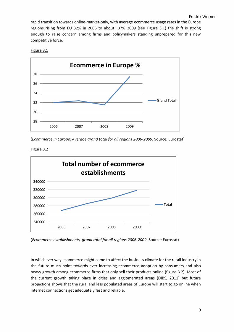
rapid transition towards online-market-only, with average ecommerce usage rates in the Europe
regions rising from EU 32% in 2006 to about 37% 2009 (see Figure 3.1) the shift is strong
enough to raise concern among firms and policymakers standing unprepared for this new
competitive force.
Figure 3.1
(Ecommerce in Europe, Average grand total for all regions 2006-2009. Source; Eurostat)
Figure 3.2
(Ecommerce establishments, grand total for all regions 2006-2009. Source; Eurostat)
In whichever way ecommerce might come to affect the business climate for the retail industry in
the future much point towards ever increasing ecommerce adoption by consumers and also
heavy growth among ecommerce firms that only sell their products online (figure 3.2). Most of
the current growth taking place in cities and agglomerated areas (DIBS, 2011) but future
projections shows that the rural and less populated areas of Europe will start to go online when
internet connections get adequately fast and reliable.
28
30
32
34
36
38
2006 2007 2008 2009
Ecommerce in Europe %
Grand Total
240000
260000
280000
300000
320000
340000
2006 2007 2008 2009
Total number of ecommerce establishments
Total
Fredrik Werner
10
Purpose of the study The main purpose of this study is to make and up to date analysis of the way that B2C
ecommerce, in broad terms being transactions between business and consumers that take place
in a non-physical-encounter manner over the internet, affects the market structure of the retail
industry in the European regions. The market structure effects that are intended to be examined
are the number of local establishments and the average employment rates. Results will be of
value for both firms and policymakers that want an empirical foundation in making future
decisions about their market positioning within the retail industry and how to act on changes in
ecommerce activity among the population.
Scope Much literature and research have focused on the US market which is in the frontline of the
ecommerce trend. Therefore the underlying purpose is not to make general findings that are of
universal importance but rather more specific for the European retail industry. Any findings will
be discussed critically and should mainly be used as a foundation for further analysis with a
more narrow sub-industry specification.
Method I will use a theoretical and empirical combination when approaching the research questions by
application of panel data regression models, specified further in the section about econometrics
and data, based on previous theoretical research. I will build the analysis on panel data built up
using Eurostat data over the European countries and regions. Without formulating my own
theoretical models the need for previously conducted studies is critical, therefore a rigorous
study of the different literature branches within economics of ecommerce is made. The
empirical modeling draws on findings in this literature.
Before setting up any econometric models to analyze the panel data with several tests are
conducted to determine what model has the best explanatory power on the dataset at hand.
This is done by running, among other, a Hausman specification tests. In all the regressions
several structures are tested against each other. Among these, dummys for each year are
included in order to handle any time trends in the data that will overthrow the ecommerce
usage rates or other independent variables effect on the dependent variable. Also region
dummy variables and other structures will be tested and evaluated before presenting the results
of the final setup.
Limitations This thesis builds on previous research and in an attempt to reconstruct the empirical
estimations made, but in a new and unexplored context. This has it’s pros and cons since it is
quite impossible to reconstruct the analysis entirely. THe main divergence that will be visible
between the reference literature and this thesis is the level of aggregation on the dataset. Due
to restrictions in time and accessibility a more aggregated dataset will be used in this thesis,
rendering the analysis a bit more general and therefore not as precise and possibly not as
accurate. The main problem that could arise with a too aggregated dataset is intensified
problems with endogenouity and the associated endogenous variable bias. Due to these
limitations in the data any analysis will be treated with care and explained in detail when made,
this to keep possible biased results out of the findings.

Fredrik Werner
11
Also the timer period covered is quite narrow and therefore merely a snapshot of the recent
years, the analysis therefore is also too be seen as a snapshot analysis where it is heightened
level of uncertainty surrounding the actual levels in the empirical modeling results. In the panel
data model specified it would have been best practice to include a lagged structure, something
that would erase possible doubts of time having a role in the data. However this is also not
possible with the short time period covered in this thesis.
In general this thesis illustrates the possibilities with panel data modeling in the market
structure and ecommerce setting. The lack of a longer time period in the data at a more detailed
level is a major limitation, but the findings presented below still make a good foundation for
further policy related research.
Literature review and theoretical background
There have been several attempts to model the way in which online retail trade and e-
commerce in general impact the market structure and the market fundamentals of existing
offline markets. Some of these theoretical findings have also to some extent been verified by
empirical tests and observations. However, as noted in Goldmanis et al (2010) the vast majority
of research papers in this area have focused on the pricing mechanisms and the effect that
better and real-time availability about prices, i.e. e-commerce diffusion, has had on industry
competition, see for example Brown et al. (2002). Much less attempts has been done to
empirically and theoretically model the firm and geographical structures of markets due to e-
commerce. The above cited paper by Goldmanis et al. is one such paper, where the composition
of firms is investigated. Another point about the overall literature is that there is an overweight
in the amount of research being done about the US markets. One reason could be that the US
has had a much more mature ecommerce sector that in relative shares of population was more
than the double compared with European countries during the peak of the last IT bubble.
(Konkurrensverket; 2001). The remainder of this section will go over some of the findings that
previous literature has found to create the foundation on which the empirical analysis then will
be built.
Ecommerce and Prices As noted above the effect of e-commerce on pricing and market prices has been more rigorously
studied than any other subject in this area. In theory ecommerce can lower the transportation
and supply-chain costs for firms shifting their marginal cost down which also means that the
profit maximizing price is lower. Lowered transaction, search or shopping costs for consumers is
also an effect and means that their demand at a given price is higher than in conventional
markets, also leading to a downwards shift in the profit maximizing price for firms operating in a
competitive market. According to Lieber and Syverson (2011) much of the work in pricing
follows these logical and straight forward assumptions about the behavior of supply and
demand in a perfect competition market. To empirically investigate pricing in ecommerce data
from price comparison sites has been used in several studies. In one such study by Brynjolfsson
and Smith (2000) evidence of reduced prices in the bookstore ecommerce is found. The nature

Fredrik Werner
12
of books being the same quality regardless of where they are bought makes them a good case to
study, this also hold for the computer memory modules market examined by Ellison and Ellison
(2005). The result that prices on these “homogenous” goods are lowered by the diffusion of
ecommerce is a verification of the conventional theories depicted above. But the results in these
empirical analyses on pricing in ecommerce markets also suggest that the early assumptions
that these markets would be frictionless never became reality. The reasons for this can be found
partly by looking at the increased information asymmetry that arises in ecommerce markets.
Ecommerce and information Asymmetry Since customers cannot inspect the good that he or she is buying until it is delivered there is a
asymmetry of information between the seller and the buyer of the “lemons” type in this market.
Since the online market is fundamentally different form the offline in that sense branding
through conventional means, such as consumer contact and brand recognition, has to be
stronger. Brynjolfson and Smith (2001)2 finds that simply having the lowest price on the good
will not yield the highest sales. Branding is very important and the success and price differences
among online (book) retailers are given by heterogeneity in consumer awareness, trust and
seller branding. Since the Brynjoflson & Smith (2001) article was written many new means of
gaining trust online has been developed, such as rating sites and openly available feedback to
sellers form prior customers, with an increasing research attention towards them, see Resnick et
al. (2006), showing how gaining trust (rating) is very important for success in sales. The
information asymmetry problem is one possible reason to why the ecommerce markets are non
frictionless as discussed above. The firms operating online are found to rarely sell just the
homogenous good at the lowest possible price but rather offer bundles of products and services
or branded products to distinguish them from other firms, creating friction and lowering the
substitutability of their product.
Ecommerce and Search Costs Since pricing, which has been in the attention so far, is not something that a firm in a
competitive market picks randomly there must be underlying mechanisms that explain why the
prices changes due to e-commerce. As noted above search cost is one such exogenous power.
Much of the ecommerce literature takes the now classic example of the travel industry as a
reference to one of the offline markets hardest hit by search cost related changes. The
traditional and often small local travel agencies served a small market with a broad spectrum of
products and had sustained decreasing margins mostly coming from commission on sales from
the airlines. When the industry saw increasing sales of tickets on the new online marketplaces
more and more of the commission that small travel agencies lived on was taken away by the
airlines. The result, verified in Goldmanis et al (2010) and Lieber & Syversson (2011) was that a
substantial part of the smaller and high cost firms dropped out of the market. Consumers and
the final good producer, in this case the airlines, understood to take advantage of the lower
search cost that arise from the internet. The search cost that previously was the revenue to local
agencies from commissions for bookings had now been possible to disregard using online
markets to book directly. The mechanism that in this case lead to exits and market share shifts
has not been observed in the same manner in any other market but market shifts due to
2 Note that there are two articles used by the authors Brynjofsson & Smith, one from 2001 and one from
2000.
Fredrik Werner
13
decreasing margins as an effect of lowered search costs is a an observed effect of ecommerce
diffusion.
The theoretical logic behind ecommerce and lower search costs for consumers is something that
is generally accepted among researchers in this field of economics (Lieber, Syverson 2011).
There are numerous examples of literature examining price-comparison sites and other
“shopbots”, see for example Ellison & Ellison (2005) and Ellison & Ellison (2006). The amount of
time needed by the consumers searching for goods from different producers and the cost
involved with this is drastically lowered by taking the search online. According to Brynjolfson,
Dick & Smith (2006) there still is some cost involved but it is considerably lower than conducting
the same search offline. Goldmanis et al (2010) and Lieber & Syverson (2011) show that the
lower search cost for consumers have an effect on several of the markets supply and demand
side fundamentals such as price, marginal cost, marginal revenue and firm composition. To
explain why this can be next a summary of the search cost model is presented.
The model on search cost and ecommerce used in this thesis comes from Goldmanis et al (2010)
who in turn draws from the large literature on search cost, see for example Carlson & McAffe
(1983) and Hortacsu & Syverson (2004), as well as general industry equilibrium literature.
Summarizing the general theoretical set up of the search cost model without going too much
into depth on the different mechanisms, the market is composed by heterogeneous demand
(consumers) and heterogeneous supply (producers) both buying and selling a homogenous
good. The supply side has a sunk cost in setting up production and a marginal cost for each good
produced if they choose to take on production in the first case. The demand side knows that
there is a price distribution for the homogenous good but have to search to find out which firms
sells for which price. The latter is the search cost component for the consumers which basically
involves going through the firms supplying the good “one by one...” (Goldmanis et al. 2010) to
get the price information needed to make a purchase decision. The consumer will keep on
searching for the best price as long as the “…expected price reduction is greater than the
marginal search cost,” . (Ibid.) This means two things for the market; first if the search cost is
high the prices in the market can also be relatively high without lowering demand, secondly if
search cost is lowered the price needs to be decreased in order to be able to sell the good. The
latter happens due the fact that consumers that face a decreasing search cost will keep on
searching for the lowest price far longer than if the search cost was higher. Or ultimately when
the search cost is zero the consumer “…always buys from the firm with the lowest price.”(Ibid.)
A quite simplified version of the conditions for this theoretical model would look like:
E(Price_reduction) > ʃ Search cost
(eq. 1)
The outcome of this model, which also differentiate it from the pricing literature presented
above, is that firms with a to high production cost will not continue or enter into production as
the search cost for consumers gets lower thereby lowering the price on the market. Firms that
can produce at a marginal cost lower than or equal to the price on the market will stay and
supply. This means that the market structure, meaning the type of firms that are active in the
market, changes as search cost and thereby prices change.

Fredrik Werner
14
Also early search cost research by Bakos (1997) with focus on the online market and how it
effects the strategies and advantages for firms and the incentives for consumers show patterns
of losses in relative competition by introducing ecommerce. Bakos sees internet as a medium for
reducing the time it takes for a buyer to find out differences among the sellers offerings. The
market that is modeled is like the Goldmanis market a monopolistic competition market with
heterogeneous sellers and goods. Their findings suggest that if the search cost gets to low in a
monopolistic competition market the equilibrium would be destabilized resulting in a possible
breakdown into perfect competition. If the perfectly differentiated market where to face ever
decreasing search costs the nature of the market would become such that all buyers would
consider all offerings at the same time and pic the one best suited for themselves. Here firms
would get the most profit by specializing their production rather than differentiating since to
many varieties of goods would mean a profit close to zero. (Bakos: 1997).
The findings in the Goldmanis et al paper suggested that smaller firms will drop out at a higher
rate due to inefficiency and larger firms would survive. This can be related to the Bakos paper in
that product differentiation would most likely render the firm in a less competitive situation due
to less economics of scale. Scale in production and reach is also the main problem for a
relatively small firm in a highly competitive market. The notion of small firms exiting is therefore
not only possible to derive from their size but rather their “production” efficiency.
Ecommerce and geography So far prices and the mechanisms such as search and transaction cost has been accounted for.
We have also looked at how the information asymmetries creates incentives for firms to engage
in more heavy branding and trust increasing activities. Now we will turn to the literature on
ecommerce diffusion and its implications on geographical and demographical structure in offline
markets.
In a more frictionless market than before consumers can “move” around at the speed of the
internet between different stores to find what they are looking form. There is some evidence
that the ecommerce markets have no boundaries and that distance is not a issue here. However
this must be taken with a pinch of salt. Even though some studies (Lieber & Syverson; 2011)
show that people living in smaller cities and rural areas will go online for shopping to a larger
extent than people living in larger urban areas, there is also evidence that the propensity to buy
decrease with distance form seller.(Hortacsu et al., 2009)
Ecommerce and its effects on- and dependence off local market structures can be seen as
something that is consumer driven. This notion comes from the fact that it is not until someone
enters the online market/store that the full benefit it generates for firms adopting the
technology is realized. Also no other effect on traditional markets is realized before consumers
start using the online marketplace, since merely adopting ecommerce technology doesn’t lower
the costs for adopting firms, giving rise to a competitive advantage. Ellison and Ellison (2006),
among other, suggest that local offline market demand and local offline market structure plays
an important role in determining the effect of ecommerce activity. If the local market is highly
competitive, with many firms competing both in price and quantity, the direct gains of adopting
a ecommerce market platform is less clear for individual firms. Allen, Clark and Houde (2008)
suggest, for the banking industry, that reducing offline activity on a more competitive market is
Fredrik Werner
15
much more risky than in less competitive markets. This activity reduction includes both
decreasing the number of personal and local establishments. In Dixon & Rimmer (2002)
evidence is found in real data simulations that the regional competitive context play an
important role in determining the effect of ecommerce. In regions where there is less local
competitiveness, occupations related to offline retail trade and firms with offline only retail
trade are much more effected than in more competitive regions. Here regional agglomeration is
used as one of the main measures for regional competitiveness levels.
Already in an early paper by Steinfield & Klein (1999) it was suggested that local markets would
matter for ecommerce even though it had a boundary-free characteristic. In the aforementioned
paper not only local market structure and competition was hypothesized as important for
ecommerce success but also cultural and regional preferences of the consumers. Therefore
regional competition between ecommerce and offline markets will be determined by the
regional consumers’ behavior rather than the choices made by the local firms. In the search cost
literature presented above, Goldmanis et al (2010) find that regions where ecommerce is more
frequently used also see higher rates of high-cost-firm dropout. This pattern could be due to the
fact that markets where ecommerce usage increases more are initially less competitive with
corresponding higher price levels and as an effect of increased competition high-cost-firms are
driven out.
The overall findings in the ecommerce and geography literature is that diffusion of ecommerce
is driven by the regional concentration and competition where firms that have higher costs, are
smaller or have lower quality will be much more effected than larger firms that have a lower
cost or higher quality. This effect will also be much larger in agglomerated areas and cities, both
because of the competitive nature of these areas but also because of trends pointing towards a
much higher ecommerce usage in these agglomerated areas (DIBS: 2011).
Firm survival and exit To give some foundations to the arguments presented about firm survival and exit in a
competitive market an brief overview of such effects in the industrial dynamics literature is in
order. In a paper by Jovanovic (1982), one of the most famous industrial dynamics authors, it is
found that the efficiency of the firm determines if it is to survive or exit the market, not only the
size and growth rate as previous research had shown at that time. Jovanovic finds that it is the
efficient firms who grow fast and thereby becomes large relative to its competitors that will
ultimately survive at a higher rate. Relating this to the ecommerce case we can see patterns of
this large firm success. Even though for some types of industries where ecommerce has been
adopted over the resent years there seems to be no relationship between the growth of the e-
commerce sector as a whole and exit of small and/or relatively inefficient firms, for example the
wholesale industry which is business to business oriented. There are still a number of industries
where a clear relationship has been found between e-commerce growth and firm exit, one being
the retail industry (Goldmanis et al. 2010). As visible in figure 1 below there is a clear temporal
relationship between increasing ecommerce activity and the number of firms in a retail oriented
market.
Figure 4

Fredrik Werner
16
(Source: Goldmanis et al. 2010)
Market effects Another part of the economic literature used in the buildup of hypothesis and research question
in this paper focus on the effects of not only cost reductions or increases for the supply and
demand sides but the transaction effects and spatial aspects of ecommerce. This literature is
less homogenous in concluding whether ecommerce has had a positive or negative effect for
certain types of firms but gives some result worth mentioning. In terms of transaction, it has
been shown that there are gains from increasing use of ecommerce that are of a supply-chain
oriented nature (Brown & Goolsbee; 2002). With less local warehousing and more scale in
transportation firms can benefit from ecommerce. This goes hand in hand with the efficiency
and firm survival presented above and would mean not only that firms that are efficient in their
production but also in their transportation (or more generally; supply) will have a relative
advantage over their competitors. A phrase much used in these settings would be “death of
distance” (Lieber & Syverson. 2011).
There are results showing that the composition of the region matters for how large the effects
of ecommerce related market outcomes will be. For example export, industry and tourism
intensive regions has been showed to gets less positive out of ecommerce than cities and more
agglomerated areas ( Dixon & Rimmer; 2002). The suggested effect can be related to the relative
competitiveness of the region but also the competition within the region as presented in the
section ‘ecommerce and geography’ above. Therefore market effect will differ and the market
outcome will thereby depend on the settings of the particular market (Dixon & Rimmer; 2002).
Research question and Hypothesis This paper draws on theoretical findings from the presented literature in formulating the main
hypotheses, recognizing the search cost literature as the less explored and more recent and
therefore taking the empirical and theoretical modeling of Goldmanis et al (2010) as the
Fredrik Werner
17
foundation for the empirical analysis. However the market focus of this thesis lies on the
European retail market rather than the more rigorously explored US market, which is the market
of focus in all of the previously presented literature. Furthermore, the empirical model includes
more background data on regional and national level than others have done in an attempt to
deepen the analysis further.
There is reason to believe that the diffusion of ecommerce in the European setting will be
different from that of the US. As previously stated the overall European technological readiness
is quite different from that of the overall US. While some countries, such as Sweden or the UK,
have come quite a bit on the way other countries such as Italy has not. (DIBS; 2011) Therefore
the novelty in this thesis hypothesis formulation will not lay in the formulation but rather the
context of which it is set to analyze.
Drawing from the previously presented literature on structural changes on a market level within
the retail industry, my first and main hypothesis is also the most straight-forward and thereby
also the least descriptive answer to the main research question: ‘How do ecommerce adoption
by consumers effect the market structure of retail firms?’.
Hypothesis 1: Ecommerce adoption and diffusion has a negative effect on the number of
establishments on a local market.
Hypothesis 2: The average firm size increase as ecommerce usage increase on a local
market.
Hypothesis 3: The regional adoption rate of ecommerce has an effect on the
establishment counts in that particular region.
Hypothesis 4: The effects of H1 differs between different markets i.e. the geographical
context matters for ecommerce.
Causation and Correlation
Before looking on the data and specifying the models that will be used to answer the research
question and hypothesizes presented above a quick review about causation and correlation is in
order. As seen in the presented literature it is clear that ecommerce have some effect on the
different parts of the retail, and other, industry. There is a clear relationship found in many of
the previously examined cases that ecommerce reduce the time and cost for both the supplier
and the consumer side. However there are always auxiliary market events that cause shifts in
the demand and supply structure of a market. The theoretical models and assumptions that
have been presented above all assume certain perfect conditions to be fulfilled. Therefore their
corresponding empirical results are all incomplete to the extent that they cannot possibly be
true for every case of analysis. The theory on search cost, which is the main source in this thesis,
assume heterogeneous producers (establishments) that compete with a dollar value per good
delivered at a given level of quality. (Goldmanis et al. 2010) Taking the analysis up to the
regional level and comparing firms within the aggregated retail industry surely means that the
producers are heterogeneous, but there might be other things such as scale advantages and
transaction advantages that play a role for the market structure.
Fredrik Werner
18
The question than is whether or not one can assume that correlation in this case also means
causation. Arguably the strongest case for that there might be causation to be found in this case
is the relative growth of overall retail trade and the ecommerce retail trade. While the turnover
growth of retailing have been decreasing (even declining) for some of the resent years
ecommerce retailing have seen nothing of this. Ever increased competition driven both by
ecommerce and by general market events such as shifts in production and transaction
technologies will decrease the possible profits to be made on a market. Ecommerce adoption
certainly plays a role in getting the consumers more aware of the different offers made by
suppliers. But it could on the other hand also be that larger and larger chain-type producers
increase the price awareness by heavy exploration of the markets and fierce pricing on the
offered goods. This would mean that the relative number of firms would in fact decrease but the
establishment figures would keep at an approximately steady rate. Therefore this is controlled
for using the employment variable in all of the specified models.
Data description
For the empirical analysis data from the European statistical directorate Eurostat are used. The
data set is gathered through their online database and put together in a panel on regional level.
A four year period is used since this was possible to construct with all available data. One of the
main problems with the data gathering was consistency in coverage. For European regional data
one possible reason to why this type of analysis has not been done previously is that there is
lack of historical data on ecommerce reported before the year 2006 for European level. Not all
countries report regional statistics to the Eurostat and not all countries that do report other
regional data has submitted regional internet statistics. There are numerous reasons for this but
one main reason becomes clear when speaking to representatives for the Swedish data
reporting to at SCB, there are strict legislation regarding publishing data about the own
country’s individuals to a foreign or supranational organization or directorate.
In the rest of this section the panel will be described in more detail and definitions of the
regional boundaries, markets and variables will be made. In the next section the empirical
analysis is presented together with the corresponding econometric models from the theoretical
section above.
Eurostat Dataset
The European dataset is gathered from the European statistical database
(http://ec.europa.eu/Eurostat). Eurostat is a sub directorate to the European Commission and
are responsible for collecting regional and national data for all member nations within the EU.
The data used was downloaded during the time period 2012-02 to 2012-04.
Industry definition
The retail industry is classified at a two digit level in the NACE classification system. The
classification cade is the same for all European countries and also follows international
standards on statistical classification. In this thesis, data for the retail industry in total as well as
some of the underlying more specific sub industry classifications of the retail industry is used,
see the variable description below for more detailed information. During 2008 some changes
were made to the industry definition, both excluding and including sub industries to the industry

Fredrik Werner
19
identification code G. Going through all of the changes made that is provided by the Eurostat a
selection of sub classes that were not altered but merely renamed or regrouped was made.
There were two industry sub classes that was removed from the retail industry in total variable,
G473(new NACE) and G527(old NACE). These alterations of the original data were made to
secure that any effects in the data would not come from possible inclusion or exclusion of new
data from year to year. Since it is of little relevance for the research question in this thesis the
complete list of changes between the sub industry classifications is available at (Industry
correspondence table) and will not be included in the appendix.
For the main research questions the data on the retail industry in total is used if nothing else is
stated. Other research papers have looked at specific parts of the retail industry trying to sort
out sub-segments that are more representative in terms of effect for the research question in
focus, see for example Goldmanis et al. (2010) and Lieber & Syverson (2011). However in this
thesis the empirical analysis has been shifted to cover a broader spectrum of firms and hence
more aggregated industry classification data is used as the main dependent industry
classification. When not specified the industry covered is the entire Retail trade industry except
for online & post-order firms.
Market Definition
The Eurostat data follows the NUTS classification system and this thesis will use data on a NUTS
2 level. This classification is corresponding with the member states highest level of regional
classification, for example Sweden is divided into 8 levels in the NUTS 2 classification and not by
the more frequently used regional level system Län which divides the country into 21 different
regions. The latter is defined as NUTS level 3 which is not used in this thesis due to data
unavailability at this level
The main reason for having data on a NUTS 2 level is that this is the level where the availability
of e-commerce data is the largest. However the availability of e-commerce data for several east-
European countries and also some of the EU members are so low (or missing in total) that these
countries are excluded from the dataset entirely. Hence the dataset consists of a sample of
European countries both members and non-members of the European Union. Also since the
Eurostat regional database section is relatively new (started 2006) and many countries therefore
have not reported any data for many of the variables. The drawback for analysis from these
exclusions and restrictions is that the results cannot be said to be representative for the whole
EU region, rather they present a descriptive selection from the different types of countries that
the region is composed of. The 20 countries included are: AT, BE, BG, CY, CZ, DK, ES, FI, HU, IE,
IT, LU, LV, NL, NO, PT, RO, SE, SK and UK. The different regions within the countries are labeled
by a geographical identification code composed of both the country code and the NUTS2 level
code. In the dataset this identification is called geoID and is the one used as the panel entity
name.
The different regions differ quite a lot in size at the NUTS2 specification level. However this
might cause the econometric results to become over representative for the relatively smaller
regions. To deal with this problem I adopt two techniques, that will be further described in the
empirical model and method section. First the model specification is made in a log log form.
Taking the log of the variables mainly have positive effects on the model specification but also
reduce the problem with the large sample differences. Second and more importantly the
specifications in this thesis follow market fixed effects modeling. As noted by Goldmanis et al.

Fredrik Werner
20
(2010) using market fixed effects means that any estimated relationship “…reflect within market
variation over time.” meaning that the market structure effects that will be studied and its
relation to ecommerce will be based on the within market variations in the different regions
over time.
Time period
The Eurostat data covers the years 2006-2009 making t=4. There is a distinctive time-series
effect in the data as a result of the global financial crisis in 2008. As a result of this it is possible
to get irrelevant results in the time series. To test this a set of all the regressions later explained
in the section econometric methods where made on the two first years isolated and then the
second two years. The results were in essence the same as the results for the four years
combined but the levels was slightly higher. This verifies that no further specification regarding
the time period needs to be done to control for the financial crisis event.
Furthermore while other papers on this topic have looked mainly on the startup and diffusion
phase of ecommerce, which took place in the US context sometime around 2001-2002. Even
though this coincided with the same event in some of the European countries, far from all
countries in the Europe region was ready at this point in time. Being a mixture of late- and early
adopter countries the time span available for study, 2006-2009, suites this market context well
since it is not only the very latest years but not the early stage years either. The time variable in
the dataset is labeled time (t) for ease of study.
Variables description
In Panel 1 the main dependent variables are establishments and employment data in the retail
industry for a selection of countries within the region. Table 2 presents an overview of all
variables in the EU panel.
EmpG_tot is a variable over the total number of employees in the offline retail sector in each
region and Est_tot is an aggregated variable covering all of the offline establishments in the
retail industry in each region. Both of these variables are sums of all firms in the industry
classification G (retail industry) with exception from sub-classifications G478, G479 and G526
which all represent online establishments or mail/post order establishments and sub
classifications that changed during the period as presented above. By excluding the sales not in
store sub-classes (see further description below) these two variables become focused on the
retail stores that sell goods in “traditional” physical stores located at a specific geographical
location. One possible problem with this offline online classification is that many stores today
are both active offline and online. However most of these firms adopt e-commerce as a parallel
or supporting activity to their offline stores making them so called hybrid firms (Lieber &
Syversson 2011). Luckily, there are still numerous firms within the pure e-commerce segment
which are sorted out by this way of exclusion for the dataset. Given the available data this is the
best aggregate classification possible trying to isolate the offline retail industry from the online
in the dataset.
Employment_total is used in all of the models to control for overall economic patterns and
market structure shifts. It total employment statistics form the different regions. Furthermore I
also use the sub classes G471 and G472 in the analysis. EmplG471 and EstablG471 (EmplG472 &
EstablG472) represent the same as employment and establishment total variables but for the
sub classes in the retail industry; grocery stores (472) and non-specialized stores (471). Theses

Fredrik Werner
21
sub sectors of the retail industry are the largest in magnitude since they comprise of all non-
specialized stores (G471) i.e. selling more than just one type of good as well as stores
specialized at selling groceries and tobacco (G472). These hold a large share of the FMCG (fast
moving consumer goods) and Durable goods which are the two main segments of retail trade.
Both of these dependent variables will be used in the same way as the Est_tot variable.
Firms that sell only online and or through post or mail order, previously
mentioned as pure ecommerce firms, are measured in the Retail_online_estab and
Retail_online_emp explanatory variables. In this classification there is no hybrid operation
firms, meaning firms that sell both offline in regular stores and online or mail-order. Therefore
this variable is useful when sorting out the online from offline firms, as described above. This
variable will be used to test whether or not geography of the firm matters also on the
ecommerce only market (i.e. online). This variable is also used as a proxy for the growth rate of
number of firms in the ecommerce sector.
The third dependent variable in the dataset is Empl_per_Establ_aver. This is
simply the employment variable divided by the establishment variable in each region. However
simple the calculation this gives an important insight and measurement on the average firm size
development in the region. This variable will be used to try and explain any firm size structure
effects. Drawing from previous findings (Goldmanis et al. 2010), evidence suggest that as
ecommerce activity among the consumers increase smaller firms will on average have a harder
time to survive then larger sized firms. This variable is also made for the respective sub classes
G471 and G472 presented above.
The main explanatory variable of interest, tracking consumer or individual ecommerce usage, is
Ecom_pop. In the report called “information society statistics” presented each year by the
Eurostat regional data on several topics concerning household usage of IT and internet are
reported. The sampling in this survey is made on national level and reported as percentage
shares of individuals to the Eurostat. This variable can also be found in previous literature but
usually takes to form of individuals in a panel group where the regional belonging of the
respondent is extracted to calculate regional levels, see for example Ellison Ellison (2005) and
Goldmanis et al (2010). The main advantage with the Eurostat data is that it is already weighted
and statistically processed percentage shares of the regional population.
The variables Size, Pop_reg16_74, EUR_HAB and PPS_HAB are all demographic and geographic
variables for the specific regions. These are used in one of the specified models to try and
describe possible patterns that differ among the regions, i.e. answering hypothesis 4. The Size
variable is the regional size in Km2 and the Pop_reg16_74 variable is the population in the age
group 16-74 in the region, meaning the age group that constitute the work-abled part of the
regional population. EUR_HAB is the regional gdp in euros per person and PPS_HAB is the
purchasing power standard per person in the region.
Table 2, Variables
Variable Name Variable description
Empl_per_Establ_aver Average employment per establishment (EmplX/EstablX)
EmpG_tot G47 and 52 TOTAL employment count, Sales not in stores excluded
EmplG471 Employment Retail sale in non-specialized stores
EmplG472 Employment Retail sale of food, beverages and tobacco in specialized stores
Fredrik Werner
22
Employment_total Total employment in all sectors in the region
Est_tot G47 and 52 TOTAL local units/establishment count, Sales not in stores excluded
EstablG471 Local units/ establishments Retail sale in non-specialized stores
EstablG472 Local units/ Establishments Retail sale of food, beverages and tobacco in specialized stores
Ecom_pop Individuals who ordered goods or services over the Internet for private use during the last 12 months, Percentage share of regional (NUTS2) total population/total households
Retail_online_emp G478+9=G526 Retail sales not in stores, Number of persons employed
Retail_online_estab G478+9=G526 Retail sales not in stores, Number of Local establishments (units)
Size km2/ size of the region
Pop_reg16_74 Population in region 16-74 years old
EUR_HAB Euro per inhabitant
PPS_HAB Purchasing Power Standard per inhabitant
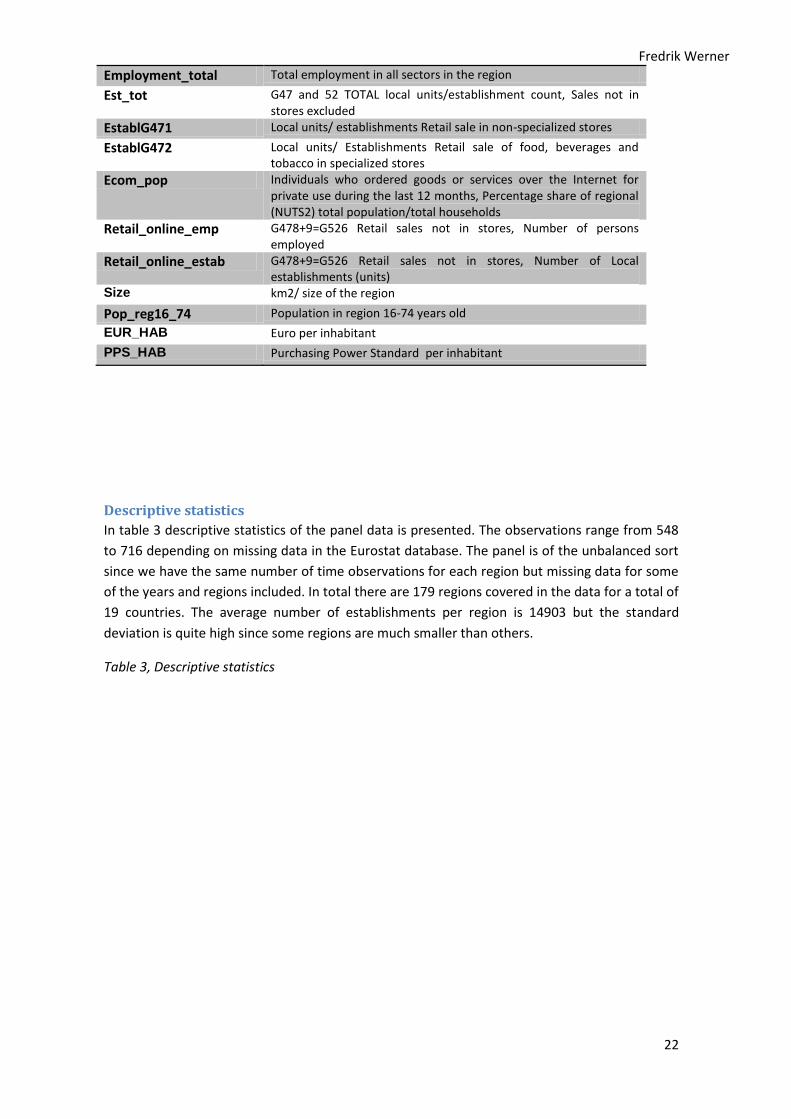
Descriptive statistics
In table 3 descriptive statistics of the panel data is presented. The observations range from 548
to 716 depending on missing data in the Eurostat database. The panel is of the unbalanced sort
since we have the same number of time observations for each region but missing data for some
of the years and regions included. In total there are 179 regions covered in the data for a total of
19 countries. The average number of establishments per region is 14903 but the standard
deviation is quite high since some regions are much smaller than others.
Table 3, Descriptive statistics
Fredrik Werner
23
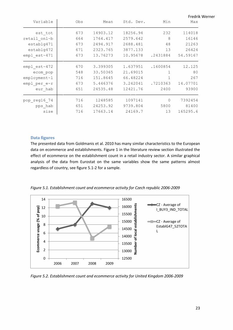
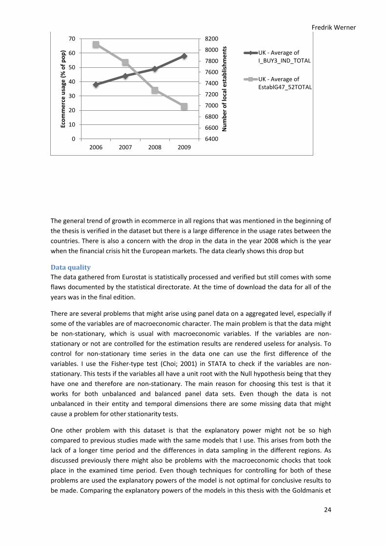
Data figures
The presented data from Goldmanis et al. 2010 has many similar characteristics to the European
data on ecommerce and establishments. Figure 1 in the literature review section illustrated the
effect of ecommerce on the establishment count in a retail industry sector. A similar graphical
analysis of the data from Eurostat on the same variables show the same patterns almost
regardless of country, see figure 5.1-2 for a sample.
Figure 5.1. Establishment count and ecommerce activity for Czech republic 2006-2009
Figure 5.2. Establishment count and ecommerce activity for United Kingdom 2006-2009
size 716 17663.14 24169.7 13 165295.6
pps_hab 651 24253.92 9739.804 5800 81400
pop_reg16_74 716 1248585 1097141 0 7392454
eur_hab 651 24535.48 12421.76 2400 93900
empl_per_e~r 673 5.446376 3.242041 .7210363 14.07701
employment~l 716 151.8645 66.48224 1 267
ecom_pop 548 33.50365 21.69015 1 80
empl_est~472 670 3.399305 1.637951 .1600854 12.125
empl_est~471 673 13.76273 10.95678 .2431884 54.59167
establg472 671 2323.765 3877.133 13 26424
establg471 673 2494.917 2688.481 48 21263
retail_onl~b 664 1764.417 2579.642 8 16146
est_tot 673 14903.12 18256.94 232 114018
Variable Obs Mean Std. Dev. Min Max
12500
13000
13500
14000
14500
15000
15500
16000
16500
0
2
4
6
8
10
12
14
2006 2007 2008 2009
Nu
mb
er
of
loca
l est
ablis
hm
en
ts
Eco
mm
erc
e u
sage
(%
of
po
p) CZ - Average of
I_BUY3_IND_TOTAL
CZ - Average ofEstablG47_52TOTAL
Fredrik Werner
24
The general trend of growth in ecommerce in all regions that was mentioned in the beginning of
the thesis is verified in the dataset but there is a large difference in the usage rates between the
countries. There is also a concern with the drop in the data in the year 2008 which is the year
when the financial crisis hit the European markets. The data clearly shows this drop but
Data quality
The data gathered from Eurostat is statistically processed and verified but still comes with some
flaws documented by the statistical directorate. At the time of download the data for all of the
years was in the final edition.
There are several problems that might arise using panel data on a aggregated level, especially if
some of the variables are of macroeconomic character. The main problem is that the data might
be non-stationary, which is usual with macroeconomic variables. If the variables are non-
stationary or not are controlled for the estimation results are rendered useless for analysis. To
control for non-stationary time series in the data one can use the first difference of the
variables. I use the Fisher-type test (Choi; 2001) in STATA to check if the variables are non-
stationary. This tests if the variables all have a unit root with the Null hypothesis being that they
have one and therefore are non-stationary. The main reason for choosing this test is that it
works for both unbalanced and balanced panel data sets. Even though the data is not
unbalanced in their entity and temporal dimensions there are some missing data that might
cause a problem for other stationarity tests.
One other problem with this dataset is that the explanatory power might not be so high
compared to previous studies made with the same models that I use. This arises from both the
lack of a longer time period and the differences in data sampling in the different regions. As
discussed previously there might also be problems with the macroeconomic chocks that took
place in the examined time period. Even though techniques for controlling for both of these
problems are used the explanatory powers of the model is not optimal for conclusive results to
be made. Comparing the explanatory powers of the models in this thesis with the Goldmanis et
6400
6600
6800
7000
7200
7400
7600
7800
8000
8200
0
10
20
30
40
50
60
70
2006 2007 2008 2009
Nu
mb
er
of
loca
l est
ablis
hm
en
ts
Eco
mm
erc
e u
sage
(%
of
po
p) UK - Average of
I_BUY3_IND_TOTAL
UK - Average ofEstablG47_52TOTAL

Fredrik Werner
25
al model it becomes clear that it is always hard with fixed effects panel data regressions to get
very strong R2 values, even with a much larger dataset there are always a risk of omitted
variables.
Empirical models and econometric method
Before going into detail about the empirical specification is important to mention that there are
some parts where the theoretical models and assumption and the model go apart. First of the
theoretical model and assumptions that are used in this thesis assume that market equilibrium
is determined simultaneously. This is an important aspect for the basic findings in the theoretical
model but very hard to instrument or implement in the empirical model. Secondly there is no
doubt that internet usage and availability is closely related to ecommerce adoption and usage.
But there is also a possibility that ecommerce availability is directly related to the internet usage
frequency in the region or country. With exception for one of the specifications below (model
1b) where the relation between adoption and availability is examined indirectly, any direct
control for “what drives what” analysis would be an own thesis in itself. Therefore the modeling
specifications are made corresponding to also the empirical models in previous research by
Lieber & syversson (2011) and Goldmanis et al. (2010).
Empirical models This paper will make some small but critical changes to the empirical test of the search cost
model created by Goldmains et al. (2010) in which the authors take total establishments by size-
class and region and an aggregated panel survey on internet usage trends in the same region as
the variable to test the models predictions. The main changes made by this paper involves the
context of the market, beeing the European regions, and the more resent time period. The
empirical models specified below draws on the findings by Goldmanis et al (2010) and Lieber &
Syverson (2011). The connections are discussed after each model and the results are later linked
in the results section.
Note that the specifications of variables are not the same in these models as they are in the
dataset and in the later econometric models. The below specifications are made to get a general
understanding about the structure of the different models that will be later specified and tested
econometrically.
Model 1a
Establishments_it = ecom_pop _it + employment_total _it
To answer Hypothesis 1 (H1) empirical model 1 is used. This model follows the specifications of
previous research on the topic and has two levels of dimension; Region (i) and time (t).
Estblishments in this model is the establishment variables, i.e. the dependent variables on total
and sub class establishment counts est_tot, establG472 and establG471, where it stands for
each region (i) and year (t).The same spcifications are used for model 3 and 4 in terms of the
three dependent variable. Ecom_pop is the percentage share of the regional population buying
online and emp_tot is used to capture market trends across all sectors of the regional economy
Fredrik Werner
26
that would otherwise be correlated with the error term. This is also the general setting that is
used as a foundation for the other models by switching dependent and independent variables.
This empirical model is specified in the same way as the Goldmanis et al. original model. The
establishment is however on a total/ aggregated level here due to the lack of firm size specific
establishment count data in the Eurostat database. The Goldmanis model is specified in a
market (i) fixed effect log-log form which is discussed more in the econometric section below. In
the original model this is made to control for any spurious results created by differences in
ecommerce growth rates in certain markets. After the discussion on the model specification
tests this same econometric model will be applied or the random effects model if it fits the data
better.
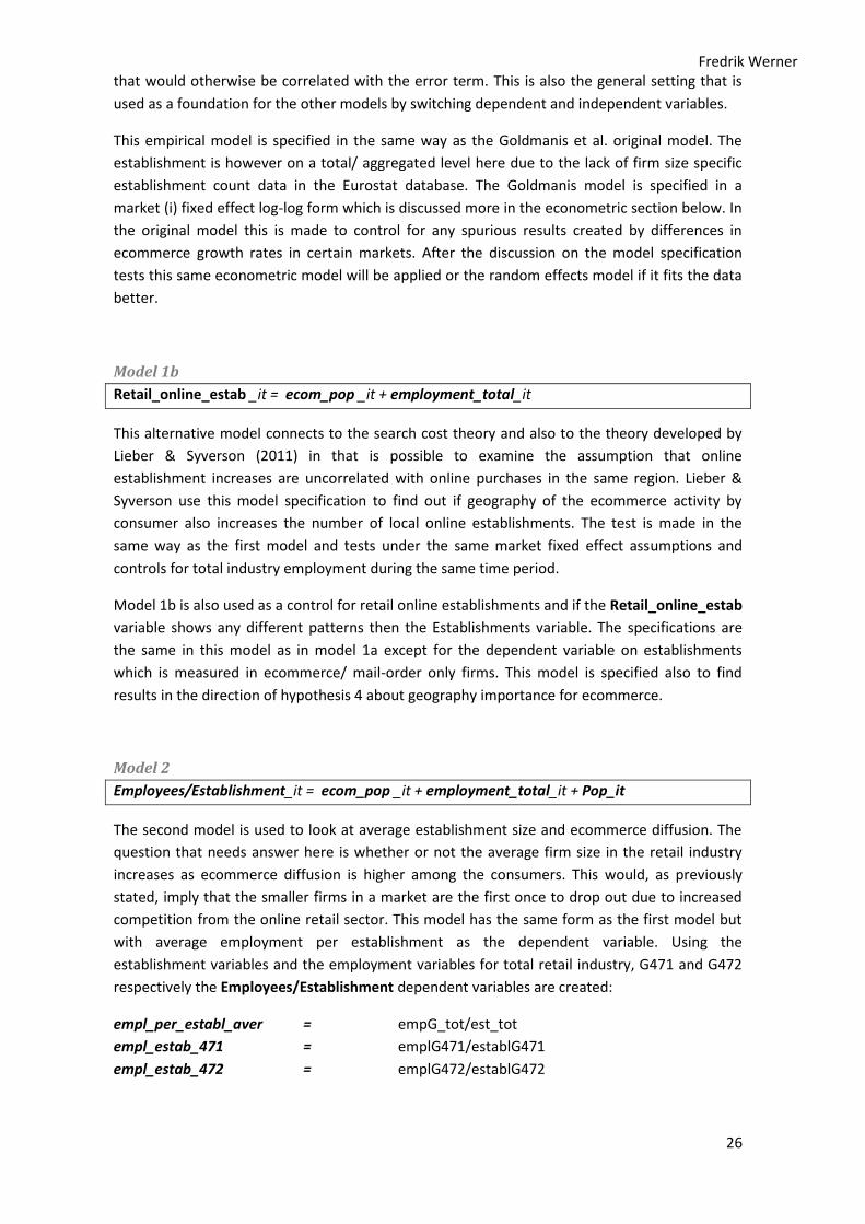
Model 1b
Retail_online_estab _it = ecom_pop _it + employment_total_it
This alternative model connects to the search cost theory and also to the theory developed by
Lieber & Syverson (2011) in that is possible to examine the assumption that online
establishment increases are uncorrelated with online purchases in the same region. Lieber &
Syverson use this model specification to find out if geography of the ecommerce activity by
consumer also increases the number of local online establishments. The test is made in the
same way as the first model and tests under the same market fixed effect assumptions and
controls for total industry employment during the same time period.
Model 1b is also used as a control for retail online establishments and if the Retail_online_estab
variable shows any different patterns then the Establishments variable. The specifications are
the same in this model as in model 1a except for the dependent variable on establishments
which is measured in ecommerce/ mail-order only firms. This model is specified also to find
results in the direction of hypothesis 4 about geography importance for ecommerce.
Model 2
Employees/Establishment_it = ecom_pop _it + employment_total_it + Pop_it
The second model is used to look at average establishment size and ecommerce diffusion. The
question that needs answer here is whether or not the average firm size in the retail industry
increases as ecommerce diffusion is higher among the consumers. This would, as previously
stated, imply that the smaller firms in a market are the first once to drop out due to increased
competition from the online retail sector. This model has the same form as the first model but
with average employment per establishment as the dependent variable. Using the
establishment variables and the employment variables for total retail industry, G471 and G472
respectively the Employees/Establishment dependent variables are created:
empl_per_establ_aver = empG_tot/est_tot
empl_estab_471 = emplG471/establG471
empl_estab_472 = emplG472/establG472

Fredrik Werner
27
Model 2 draws on the basic theoretical notion that the smaller the firm the more effected it will
be by increased competition. This is something that Goldmanis et al measures on an exact level
in their model by including per size-class establishment counts. There are drawbacks in the use
of the average employment per establishment variable in that the average could be left
unchanged if the larger firms absorb the employees of the smaller firms as they exit the market.
Model 3
Establishments_it = ecom_pop _it + employment_total_it + time_dummies_t
This third model is used to answer Hypothesis 3; if there is any between market differences in
how ecommerce adoption growth rates effect establishment counts. This model tests if markets
with higher than average ecommerce growth rates also see higher than normal effects on
establishment counts. This is made possible by the time dummies that isolate the within market
effects also over time and from aggregate shifts in the variables. A positive coefficient on the
independent variable ecommerce_usage would in this case imply that markets with below
average decreases in establishments also have lower than average increases in ecommerce
adoption rates. This is a good measure to see if there is anything about the ecommerce
adoption rate itself hat effect the establishment count rate i.e. if there is an increased effect of
ecommerce diffusion on establishments and local competition in regions or if the effect of
ecommerce diffusion takes place on a aggregated level and that any regional differences depend
more on the regional settings then the rate of ecommerce growth.
Model 4
Establishments_it = ecommerce_usage _it + employment_total_it + N_it
In the model number 4 the main addition from the first is the variable N which is a set of
regional and country specific background variables. The latter group is composed by the set of
regional variables that were presented in the DATA section above and will therefore only be
printed out in the regression results tables and the empirical analysis when necessary. This
model is used to further investigate any factors that determine the effect of ecommerce activity
on a regional and aggregated level using both regional dimension model and country dimension
model. The main purpose of the model is to answer hypothesis 4 which is about possible
underlying or aggregated characteristics that differs among the regions and that affects the
impact of ecommerce on establishments.
Econometric method The variables have two dimensions regional and temporal. Since predictors are on two different
levels a standard OLS regression is not valid. The problem that would arise is that variables that
are nonrandom would be regressed as if they were random. This would violate the basic OLS
assumptions and possible overestimation of the regression results. It would in practice be like
saying that all regions just happened to have the same value on the aggregate variable
something that is highly unlikely. To analyze this data a different approach has to be taken than
a regular OLS regression.
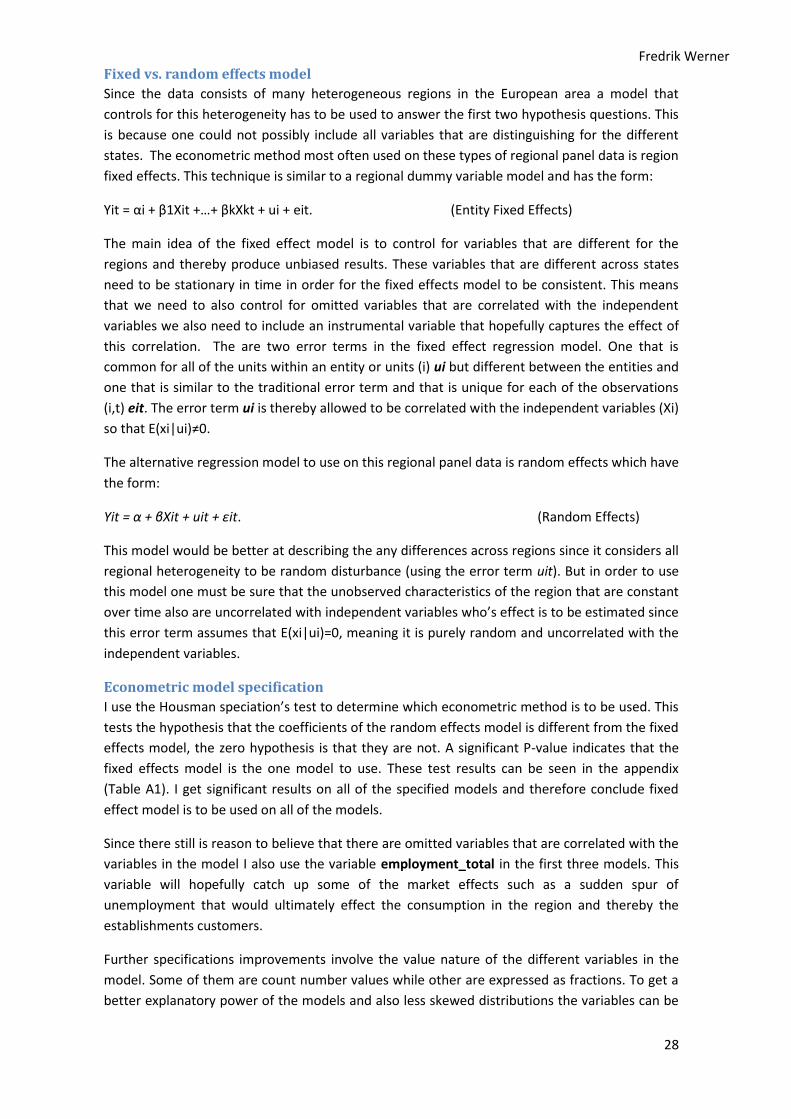
Fredrik Werner
28
Fixed vs. random effects model
Since the data consists of many heterogeneous regions in the European area a model that
controls for this heterogeneity has to be used to answer the first two hypothesis questions. This
is because one could not possibly include all variables that are distinguishing for the different
states. The econometric method most often used on these types of regional panel data is region
fixed effects. This technique is similar to a regional dummy variable model and has the form:
Yit = αi + β1Xit +…+ βkXkt + ui + eit. (Entity Fixed Effects)
The main idea of the fixed effect model is to control for variables that are different for the
regions and thereby produce unbiased results. These variables that are different across states
need to be stationary in time in order for the fixed effects model to be consistent. This means
that we need to also control for omitted variables that are correlated with the independent
variables we also need to include an instrumental variable that hopefully captures the effect of
this correlation. The are two error terms in the fixed effect regression model. One that is
common for all of the units within an entity or units (i) ui but different between the entities and
one that is similar to the traditional error term and that is unique for each of the observations
(i,t) eit. The error term ui is thereby allowed to be correlated with the independent variables (Xi)
so that E(xi|ui)≠0.
The alternative regression model to use on this regional panel data is random effects which have
the form:
Yit = α + βXit + uit + εit. (Random Effects)
This model would be better at describing the any differences across regions since it considers all
regional heterogeneity to be random disturbance (using the error term uit). But in order to use
this model one must be sure that the unobserved characteristics of the region that are constant
over time also are uncorrelated with independent variables who’s effect is to be estimated since
this error term assumes that E(xi|ui)=0, meaning it is purely random and uncorrelated with the
independent variables.
Econometric model specification
I use the Housman speciation’s test to determine which econometric method is to be used. This
tests the hypothesis that the coefficients of the random effects model is different from the fixed
effects model, the zero hypothesis is that they are not. A significant P-value indicates that the
fixed effects model is the one model to use. These test results can be seen in the appendix
(Table A1). I get significant results on all of the specified models and therefore conclude fixed
effect model is to be used on all of the models.
Since there still is reason to believe that there are omitted variables that are correlated with the
variables in the model I also use the variable employment_total in the first three models. This
variable will hopefully catch up some of the market effects such as a sudden spur of
unemployment that would ultimately effect the consumption in the region and thereby the
establishments customers.
Further specifications improvements involve the value nature of the different variables in the
model. Some of them are count number values while other are expressed as fractions. To get a
better explanatory power of the models and also less skewed distributions the variables can be

Fredrik Werner
29
express in their logarithmic form. This is done it is also specified by a L(Xit) in the regression and
results section. Looking at figure 6.1 and 6.2 below the before and after log transformation
clearly helps with the skewness of the data.
Figure 6.1 and 2 (1; before and 2; after)
The choice and composition of econometric model will also depend on what the research
question is and what the purpose of the regression is. Since the overall aim here is to examine
the causes of regional ecommerce activity changes on the regional establishment counts this
goes in line with the features of the fixed effect model. As described by Kohler & Kreuter (2009)
the “…fixed effects models are designed to study the causes of changes within a person”. If on
the other hand one which to examine if the differences across units do effect the dependent
variable it is better to use the random effects model. In model4 we are interested in the
between-region differences and therefore a random effects model is better to use here.
Including as many variables as possible that describe the individual (regional) differences is
needed in order to make this regression model work. But since it is not possible to include all
possible variables that effect the establishment and employment counts in the regions there is a
possibility that there will be omitted variable bias in the model.
The variables in the empirical models 1a and 1b and the structure of the models themselves are
constructed in the same way as Goldmanis’s original version. The specifications of these are not
changes due to the fact that this thesis draws on the same theoretical notions about ecommerce
and its effects on markets and search cost. Goldmanis et al adopt two types of fixed effects
models in their paper, one primary with fixed entity/ region specification and one temporal fixed
effect. As previously concluded fixed effects modeling is better suited for analysis of the
European data covered in this paper. The variables described are the one thing that differs
slightly form the Goldmanis model. Where they use household survey’s on ecommerce usage
gathered by Forrester research and calculate aggregated fractions in the respective regions, in
their case US counties, this thesis uses already aggregated statistics gathered by the national
statistics organizations and compiled by Eurostat. Also this thesis takes establishments in a
broader context including all of the retail trade except of retail trade, as previously presented in
the data section.
Econometric model 2 and 3 is based on the same core fixed effects modeling but draws
structural form from previous attempts on further analysis of the ecommerce and market
structure made by Lieber & Syverson (2011). In the aforementioned paper there are little to
none specifications made about the modeling per se but they are clearly pointing out that they
also build their analysis and modeling on Goldmains’ previous work.
0
2.0
e-0
54
.0e-0
56
.0e-0
5
Den
sity
0 50000 100000EstablG47_52TOTAL
0.1
.2.3
.4.5
Den
sity
4 6 8 10 12Lest_tot
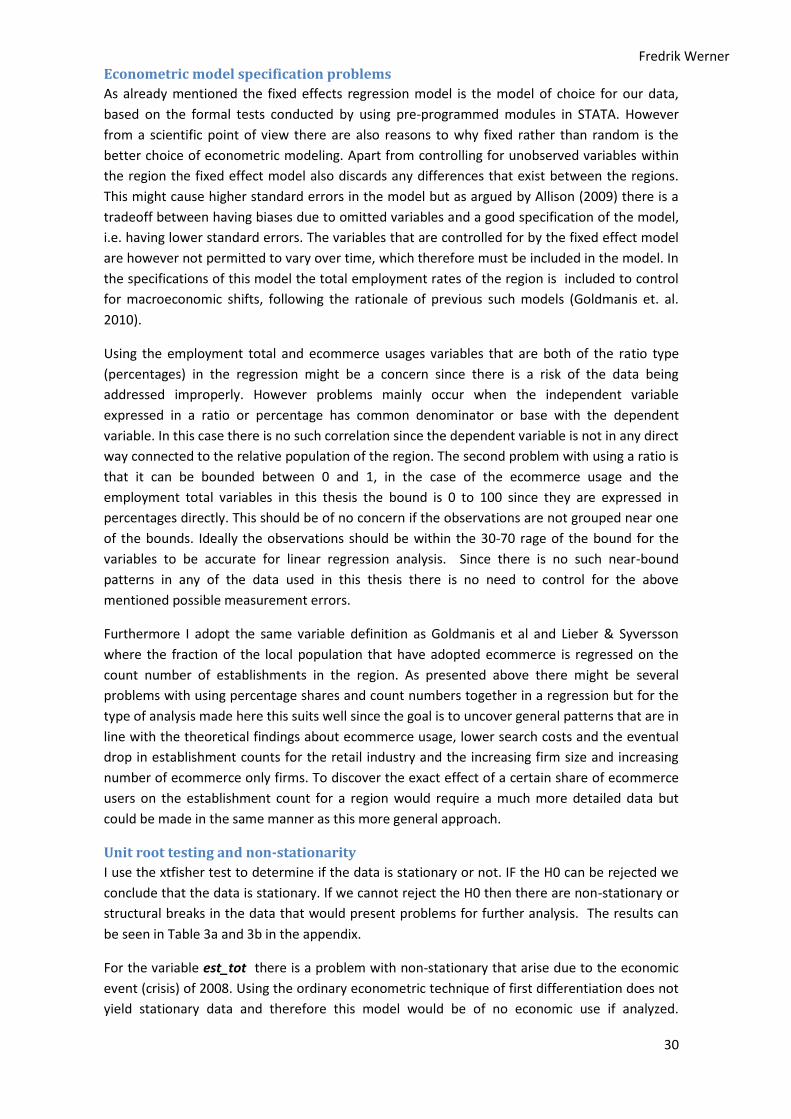
Fredrik Werner
30
Econometric model specification problems
As already mentioned the fixed effects regression model is the model of choice for our data,
based on the formal tests conducted by using pre-programmed modules in STATA. However
from a scientific point of view there are also reasons to why fixed rather than random is the
better choice of econometric modeling. Apart from controlling for unobserved variables within
the region the fixed effect model also discards any differences that exist between the regions.
This might cause higher standard errors in the model but as argued by Allison (2009) there is a
tradeoff between having biases due to omitted variables and a good specification of the model,
i.e. having lower standard errors. The variables that are controlled for by the fixed effect model
are however not permitted to vary over time, which therefore must be included in the model. In
the specifications of this model the total employment rates of the region is included to control
for macroeconomic shifts, following the rationale of previous such models (Goldmanis et. al.
2010).
Using the employment total and ecommerce usages variables that are both of the ratio type
(percentages) in the regression might be a concern since there is a risk of the data being
addressed improperly. However problems mainly occur when the independent variable
expressed in a ratio or percentage has common denominator or base with the dependent
variable. In this case there is no such correlation since the dependent variable is not in any direct
way connected to the relative population of the region. The second problem with using a ratio is
that it can be bounded between 0 and 1, in the case of the ecommerce usage and the
employment total variables in this thesis the bound is 0 to 100 since they are expressed in
percentages directly. This should be of no concern if the observations are not grouped near one
of the bounds. Ideally the observations should be within the 30-70 rage of the bound for the
variables to be accurate for linear regression analysis. Since there is no such near-bound
patterns in any of the data used in this thesis there is no need to control for the above
mentioned possible measurement errors.
Furthermore I adopt the same variable definition as Goldmanis et al and Lieber & Syversson
where the fraction of the local population that have adopted ecommerce is regressed on the
count number of establishments in the region. As presented above there might be several
problems with using percentage shares and count numbers together in a regression but for the
type of analysis made here this suits well since the goal is to uncover general patterns that are in
line with the theoretical findings about ecommerce usage, lower search costs and the eventual
drop in establishment counts for the retail industry and the increasing firm size and increasing
number of ecommerce only firms. To discover the exact effect of a certain share of ecommerce
users on the establishment count for a region would require a much more detailed data but
could be made in the same manner as this more general approach.
Unit root testing and non-stationarity
I use the xtfisher test to determine if the data is stationary or not. IF the H0 can be rejected we
conclude that the data is stationary. If we cannot reject the H0 then there are non-stationary or
structural breaks in the data that would present problems for further analysis. The results can
be seen in Table 3a and 3b in the appendix.
For the variable est_tot there is a problem with non-stationary that arise due to the economic
event (crisis) of 2008. Using the ordinary econometric technique of first differentiation does not
yield stationary data and therefore this model would be of no economic use if analyzed.

Fredrik Werner
31
However the use of non-stationary data in macroeconomic panels is a topic that has been
discussed among economists after the financial crisis. IMF’s Olivier Blanchard (Blanchard: 2009)
is one of them who in contrary to prior thoughts that this would not be consistent with
statistical theory argues that after the economic crisis of 2008 we have seen no upswing in the
economy, meaning that there seems to be a macroeconomic shift in the overall economy if the
crisis is hard enough. If following the thoughts of Blanchard we could use this variable for
estimation even though there is a structural break in the data.
The problem with non-stationary data however only resides in the overall retail industry
establishment data and not in the two sub sectors of the retail industry that are included in the
data set. These are sub segments G471 (retail sales in non-specialized stores) and G472 (retail
sales in of food, beverages and tobacco in specialized stores) described in the variables section.
Since these two variables are stationary in their log and square form they will be used in the
model 1a alternative dependent variables specifications to see if the est_tot could tell the true
story even though it has a structural break. Thereby also confirming Blanchard’s statement and
possibly confirm that macroeconomic variables could be used if the structural break is known to
be there for a reason.
Econometric variables and model specifications
Before looking at the final form of the econometric specifications some graphical examples of
the before (figure 7) and after (figure 8) transformation of the variables are presented. Since
there is a curve linear relationship in the data that needs to be dealt with the squared form of
the variables are used. This is typically used for economic variables since it is logical to assume
that there is an underlying non-linear relationship in the ‘typical economy’ that arise due to
business cycles, trends or scale economies in production. Also since we have concluded using
the fisher test that the data is non-stationary the logged form of the model is used rather than
the linear to control for non-stationary data. The second scatter graph (figure 4) shows that the
logged and squared data has a much better structure and is therefore better suited for the final
analysis.
Figure 7
. scatter est_tot ecom_pop
0
500
00
100
00
01
50
00
0
Esta
blG
47
_5
2T
OT
AL
0 20 40 60 80I_BLT12_%pop
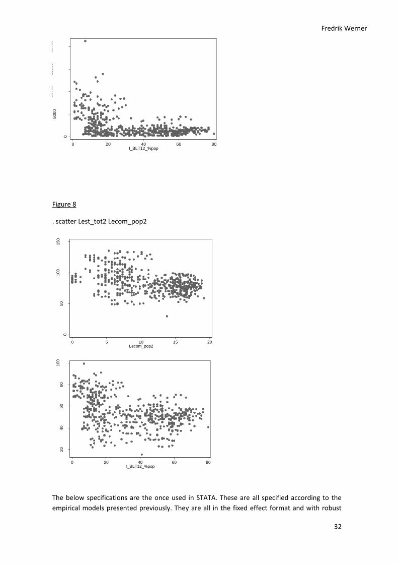
Fredrik Werner
32
Figure 8
. scatter Lest_tot2 Lecom_pop2
The below specifications are the once used in STATA. These are all specified according to the
empirical models presented previously. They are all in the fixed effect format and with robust
0
500
01
00
00
150
00
200
00
Esta
blG
47
1
0 20 40 60 80I_BLT12_%pop
05
01
00
150
Lest_
tot2
0 5 10 15 20Lecom_pop2
20
40
60
80
100
Lesta
blg
47
12
0 20 40 60 80I_BLT12_%pop

Fredrik Werner
33
standard errors. Model 3 is the only model where time fixed effects are used. All of the other
models region (entity) fixed effects are used. All variables are in Log and ^2(squared) for,
denoted by L X 2 or L2 X. The variable denotation it stands for regions and time except for model
3 where time is dropped due to time fixed effects and also ‘model 4 alternative’ where the i is
changed from region to country level.
Model 1
Y it = αi + β1Lecom_pop2 it + β2Lemploymnet_total2 it+ uit + eit.
Where Y = Lestablg4712
Lestablg4722
Lest_tot2
1b) Lretail_online_estab2
Model 2
Y it = αi + β1Lecom_pop2 it + β2Lemploymnet_total2 it + uit + eit.
Where Y = Lempl_per_establ_aver2
L2empl_estab_471
L2empl_estab_472
Model 3
Y i = αi + β1Lecom_pop2 i + β2Lemploymnet_total2 I + i.time + vi+ eit.
Where Y = Lestablg4712
Lestablg4722
Lest_tot2
Model 4
Y it = αi + β1Lecom_pop2 it + β2Lemploymnet_total2 it + β3 Leur_hab2 it + β4 Lpop_reg16_742
it + β5 Lpps_hab2 it + β5 Lsize2 it + uit +eit.
Where Y = Lestablg4712
Lestablg4722
Lest_tot2
Model 4 alternative:
Y it = αi + β1Lecom_pop2 it + β2Lemploymnet_total2 it + β3 Leur_hab2 it + β4 Lpop_reg16_742
it + β5 Lpps_hab2 it + β5 Lsize2 it + uit +eit.
Where Y = Lest_tot2
Here i refers to countryID rather than geoID like in all other specifications.
In stata commands for the fixed effects regression:

Fredrik Werner
34
Xtreg Y X, fe robust i(ID)
Expected coefficients
Here the different hypothesis and the corresponding expected econometric coefficients are
explained in short before going into the results. The estimatimated values are then presented in
the results section. The expected coefficients are presented as greater than zero or less than
zero because the sign is what is important for analysis. The values of the slop coefficients are
merely used to illustrate the results in the result analysis section.
H1
H1: suggests that B2 < 0 for the est_tot = a + b2 ecom_pop + b3 empl_tot + e
I.e. this would suggest that the firms profits are search cost elastic. I.e increase in ecom leads to
a declining number of firms in the local market.
H1b: suggests that B2 > 0 for the online_est_tot = a + b2 ecom_pop …. + e. This tests if the local
market ecommerce usage rates are important for local online only establishments. If there is a
positive sign on the coefficient we can conclude that it is.
H2
H2: B2 > 0 is expected as average firm size would increase if mostly smaller firms exit the market
and larger firms don’t. The model is on average employees/establishment in the retail industry
and how ecommerce is related to this. The expected value > 0 is derived form the theoretical
and empirical finings of previous research by Goldmanis et al. (2010).
H3
H3: if B2 < 0 then firm count decline more in regions where ecommerce activity increases
relatively more. IF B (x) time* is significant and diminishing ( Bx < 0 ) then there is a general
trend and nothing specific about the different growth rates of ecommerce that explain different
levels of establishment count shifts.
H4
H4: Any coefficient Bx that is significant when the B2 (ecom_pop) coefficient is < 0 and
significant will help explaining the effect of ecommerce activity on local establishment declines.
The alternative version of the model uses the same coefficients but looks at a country level. If
the alternative B2 < 0 is significant and the regional is not (or weak) then we can conclude that
the decline in firms cannot be explained by regional differences but rather by country
differences.

Fredrik Werner
35
Results and tables
Model 1 to 4 results with respective dependent variables specifications in at the top denoted by
a number in parenthesis.
MODEL 1
(1) (2) (3) (4)
VARIABLES Lest_tot2 Lestablg4712 Lestablg4722 Lretail_online_estab2
Lecom_pop2 -0.457*** 0.279*** -0.262*** 0.773***
(0.0873) (0.0990) (0.0641) (0.141)
Lemployment_total2 0.166** -0.327** 0.152** 0.281**
(0.0799) (0.139) (0.0722) (0.110)
Constant 86.05*** 58.89*** 50.76*** 31.96***
(2.664) (3.796) (2.112) (3.772)
Observations 537 537 535 532
R-squared 0.171 0.074 0.088 0.076
Number of geoID 177 177 177 177
Robust standard errors in parentheses
*** p<0.01, ** p<0.05, * p<0.1
MODEL 2
(1) (2) (3)
VARIABLES Lempl_per_establ_aver2 L2empl_estab_471 L2empl_estab_472
Lecom_pop2 0.150*** 0.280*** 0.0189
(0.0154) (0.0445) (0.0204)
Lemployment_total2 0.0169 -0.0416 0.00116
(0.0178) (0.0465) (0.0142)
Constant 0.632 4.033*** 1.242**
(0.541) (1.227) (0.491)
Observations 537 537 534
R-squared 0.289 0.179 0.005
Number of geoID 177 177 176
Robust standard errors in parentheses
*** p<0.01, ** p<0.05, * p<0.1
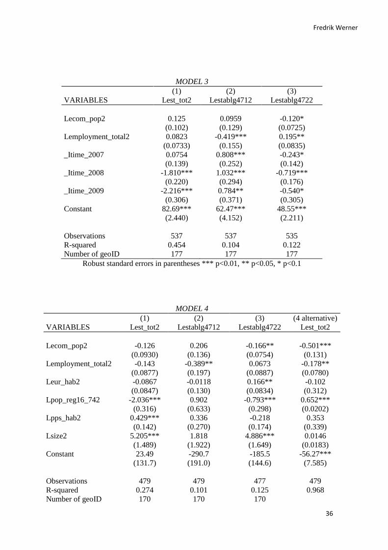
Fredrik Werner
36
MODEL 3
(1) (2) (3)
VARIABLES Lest_tot2 Lestablg4712 Lestablg4722
Lecom_pop2 0.125 0.0959 -0.120*
(0.102) (0.129) (0.0725)
Lemployment_total2 0.0823 -0.419*** 0.195**
(0.0733) (0.155) (0.0835)
_Itime_2007 0.0754 0.808*** -0.243*
(0.139) (0.252) (0.142)
_Itime_2008 -1.810*** 1.032*** -0.719***
(0.220) (0.294) (0.176)
_Itime_2009 -2.216*** 0.784** -0.540*
(0.306) (0.371) (0.305)
Constant 82.69*** 62.47*** 48.55***
(2.440) (4.152) (2.211)
Observations 537 537 535
R-squared 0.454 0.104 0.122
Number of geoID 177 177 177
Robust standard errors in parentheses *** p<0.01, ** p<0.05, * p<0.1
MODEL 4
(1) (2) (3) (4 alternative)
VARIABLES Lest_tot2 Lestablg4712 Lestablg4722 Lest_tot2
Lecom_pop2 -0.126 0.206 -0.166** -0.501***
(0.0930) (0.136) (0.0754) (0.131)
Lemployment_total2 -0.143 -0.389** 0.0673 -0.178**
(0.0877) (0.197) (0.0887) (0.0780)
Leur_hab2 -0.0867 -0.0118 0.166** -0.102
(0.0847) (0.130) (0.0834) (0.312)
Lpop_reg16_742 -2.036*** 0.902 -0.793*** 0.652***
(0.316) (0.633) (0.298) (0.0202)
Lpps_hab2 0.429*** 0.336 -0.218 0.353
(0.142) (0.270) (0.174) (0.339)
Lsize2 5.205*** 1.818 4.886*** 0.0146
(1.489) (1.922) (1.649) (0.0183)
Constant 23.49 -290.7 -185.5 -56.27***
(131.7) (191.0) (144.6) (7.585)
Observations 479 479 477 479
R-squared 0.274 0.101 0.125 0.968
Number of geoID 170 170 170

Fredrik Werner
37
Number of countryID 18
Robust standard errors in parentheses *** p<0.01, ** p<0.05, * p<0.1
Result analysis
General The biggest concern as for the regression results is the generally low values for the R2. This is
the explanatory value and should be reasonably high if the model is correctly specified.
However, with panel data scientists are usually satisfied with about 10% R2 for their results. This
might sound somewhat strange but in panel data analysis there are so many factors that could
affect the independent variables themselves differently since there are a also large number of
regions (panels) in the data. There is less exact science about the R2 values in panel data
modeling than other regression models since it is a mixture of cross-section and time-series
data. In the regression results given by STATA there are three R2 values and one Rho value. The
three R2 values are; within, between and overall. The R2 that is used here is the within value.
Even though for this thesis we are mostly interested in the within market effect of ecommerce
usage on local establishment, which would be represented by this R2 value, the overall
explanatory value of the model is the one R2 that we evaluate. This is one of the reasons to why
R2 values of around 10% are most often good news (See
http://www.stata.com/statalist/archive/2003-05/msg00336.html; (2012) for further examples
on this topic). The Rho value is known as the interclass correlation and tells us how much of the
variation is due to differences across the entities or regions in the panel. The Rho values for
most of the models in this thesis are around 0.9 which is quite high. However there is also a very
heterogeneous type of panel where one would expect the variances to be higher across regions
than within the specific regions during the four year time period that is covered. This is also
partly mended by the fact that we treat the error terms as correlated across regions in the basic
assumtions (i.e. E(xi|ui) ≠ 0 ).
When running a fixed effects regression in STATA using the xtreg command an automatic F-test
(Prob > F) is also done in order to determine if the models coefficients are different than zero.
All of the results are reported below 0.05 and therefore it is possible to conclude that the model
specifications are proper.
As previously mentioned the levels of the estimated coefficients are not to be too deeply
analyzed since they are covering macroeconomic variables over a quite small time period with
on a heterogeneous panel. The main indicators should be the sign and relative levels of the
coefficients. Since we treat all of our variables in logged and squared for the levels are to be
interpreted as follows: If the coefficient of the independent variable is -0,5 then a 1% increase in
that independent variable corresponds to a 0,5 decrease in the dependent variable. This holds
for all of the models since they are in log-log format, i.e. logarithmic in both the dependent and
independent variables.

Fredrik Werner
38
As discussed in the Causation and Correlation section the employment variable emp_tot was
used to control for market structure shifts that arose from larger establishments driving out
smaller establishments through scale in their production, amongst other reasons. Since the
relative value of the establishment count and employment numbers do not differ substantially
where they have different signs and are significant there seems like the growth in average firms
size in the market is correct but the decline in establishments is not only driven by declines in
small and increase in large firm. However this is a point that needs to be noted when reading
the results of this thesis since there is no direct way of controlling for all of the variables that
lead to market structure shifts.
Model 1 The results of model 1 confirm the theoretical assumptions and the formulated hypothesis that
ecommerce activity actually decreases the establishment counts in the regions. This effect holds
true for total establishments, where we are to be careful with our interpretations of the results
due to non-stationarity, but also for the subclass G472 (retail sales of FMCGs). However there
seems like sub class G471 (non-specialized stores) do not confirm what is predicted. The R2 for
both of the sub classes are low but still at around 8%. The result here that really proves the
theoretical notion is that the patterns for pure ecommerce establishments are quite the
opposite to the total retail industry and stronger then both the sub classes G471 and G472. If
the level of ecommerce activity among the population increases with 1%, as many as 0,773%
more establishments within the ecommerce only sector will appear in the region. Taking these
two results, about the negative for total and positive for ecommerce only establishments,
together the regressions suggest that the Goldmanis theory of decreasing numbers of local
establishments due to ecommerce diffusion holds. Also the Lieber & syversson findings about
increasing numbers of ecommerce firms within the local market as local ecommerce usage
increases is verified to some extent. However the effect in Lieber & Syverssons (2011) model is
much stronger with an increase of about 2.2 firms for every 1% increase in ecommerce usage.
Model 2 In model 2 the question was to discover if one could see any of the effects that Goldmanis found
about differences across firms of different size. The results suggest that these findings are true
also in the European setting given that we exclude G472 which has no significant coefficients.
The overall findings here is that increasing ecommerce usage has an effect on the average firm
size within the retail sector in general and the sub class G471 in particular. An 1% increase in
ecommerce usage has a 0.15 % increasing effect on the average number of employees within
the retail sector. The original model was constructed so that the different sizes of firms would
be modeled independently. There it became obvious that the smaller firms dropped out of the
market at a higher rate but that the larger firms actually grew when people started going online
to shop for their goods. This is not a replication of the original test but the results could be used
as a hint toward such a pattern also for the European context. Model 2 present satisfactory R2
values at 0.289 (retail industry total) and 0.179 (G471). There is reason to be somewhat cautious
with the results since there was a higher than normal shakeout of firms of the more risky sort
during the financial crisis which would be a possible source of spurious regression results.
The results are not comparative as such with previous results since the model is developed as a
generalization of the original size specific regression models by Goldmains et al (2010). As stated
Fredrik Werner
39
above, the verification of the original model is needed before anything definitive could be said
about the increasing firm size in the regions of Europe.
Model 3 By using time fixed effects, meaning that time dummy variables are used , every year is isolated
and a regression is made on the regional effect of all of the regions in that particular year. In
other words this model describes any within market effect that is not due to any trends or
general patterns that is the same for all regions. The findings that the variables are not
significant when introduced with a time fixed effects model means that there are no regional
specific differences in the effect on establishments of increasing regional ecommerce usage.
Instead the patterns seen in model 1 and 2 are derived from a aggregated level. On what level is
left unexplained by this model but is dealt with in the alternative version of model 4. The results
of the time fixed effects regression must be dealt with some care since the time rather than the
region fixed effect model is vounrable to omitted variable bias. The control variable on overall
economic setting, total employment, turns up significant on both of the sub classes used in
model 3. This suggests that there is something in the region’s economic settings that change
during the time periods and therefor region fixed effects model might still be more explanatory.
In model 4 we address the problem of regional adoption rates again using fixed region effects
and control variables on geographical and demographics.
The findings in model 3 regression is similar to those made by Goldmais et. al.(2010). However
where they produce no significant variables in their model the models on this data do for some
of the variables. The interesting similarity to note is that both the original version and the
version in this thesis finds that regional differences in the ecommerce adoption rates cannot
describe any of the regional differences in local establishment counts. It is therefore possible to
conclude that even though local competition is important for the firms ability to cope with local
upswings in ecommerce activity it is even more important with the aggregated ecommerce
usage patterns.
Model 4 The fourth model is constructed to try and answer if there are any region specific characteristics
in terms of geography or demography that has an effect on the impact of ecommerce diffusion
among the consumers on establishments. At a region level the results for the ecommerce usage
total coefficient are non-significant when including the different region specific variables. This
means that none of the variables included has an joint effect with ecommerce in the regional
setting, i.e. the ecommerce usage variable loses its explanatory power when these variables are
introduced in the model. The establishment count seems to be negatively affected by size and
population in the ecommerce total results. For sub class G471 there is no significant coefficient
except for total employment and the sub class G472 follows the general establishment total
patterns. However the really interesting results are to be found in the alternative model. This
model uses countries rather than regions as the panel ID and thereby the effect of ecommerce
on establishments is analyzed group wise on a country level. Goldmanis et al. (2010) finds no
patterns of relatively high regional establishment decreases and corresponding patterns in
regional ecommerce in the US and conclude that the lowered search cost and ecommerce
market effects act on a more aggregated national level. The results in the alternative model 4
tell a similar story. Both the explanatory powers of the model (R2 = .96) and the significant
Fredrik Werner
40
coefficients of the variables are increased when grouping on country level is used. The strong
results point towards ecommerce market effects being a country level phenomenon that is best
explained by looking at the entire country level. As already seen in the results of model 3
different levels of ecommerce activity rates does not explain differences between regions local
establishments so even though there are large differences within the countries in terms of
employment and market competition the effect of ecommerce apparently acts on a higher level.
These results would suggest that the most of the ecommerce effects can be derived from which
country the region is located in, which in turn implies that regional policies are less effective
than national policies. A 1% increase in ecommerce activity within a country would also mean an
average decrease of 0,5% in number of firms in the regions of the country. The effect seems also
to depend on how large the regions in the country are, with a 0,6 % increase in the number of
firms for every 1% increase in the population (above the normal population growth rate average
during the four years covered).
Comments and conclusion It is obvious that there is an effect of ecommerce diffusion on local establishment decreases in
the retail sector, even though the effect is not very strong. The main reason to the relationship
between ecommerce and firms exit could be that the retail industry markets are forced, by
lower search costs among the consumers, to move away from monopolistic competition
settings. Where previously the profits were high enough to sustain even inefficient firms there is
now only room for the most efficient ones. In most cases the first firms to drop out from a
monopolistic competition market are smaller firms with less scale economies to their favors.
This is illustrated by the increasing average size (model 2) of the local establishments which also
reflects that scale is of importance for surviving firms. Since the average firm in the traditional
retail sector is found to increase in size as ecommerce use increases the market structure will
become even tougher for possible entrants in the future.
Concluding on which is more important; local or aggregated patterns, is hard since there are
some results speaking partly against each other. On the one hand the ecommerce activity is
important and has a decreasing effect on the local establishments. Also local online only
establishments thrive in the presence of increasing local ecommerce usage by consumers.
However there seems like the relative ‘growth rate’ or differences in the rate at which local
consumers use ecommerce in the different regions in unrelated to any differences in the
establishment dropout rate in a regional context. So what could be concluded is that the
regional context matters for the startup of new ecommerce only establishments but the market
structure shift in the traditional (offline) retail industry comes from a more aggregated shift in
ecommerce usage. This suggests that there is a positive effect of local ecommerce activity on
regional online establishments that translates over to the country level as seen in model 4,
where in turn the market structure shift takes place for the traditional establishments.
Furthermore this suggest that the regions with a higher rate of adoption, which in most cases
are more agglomerated areas, acts as growing grounds for the ecommerce establishments
which then in turn effect the market shares of traditional firms in other regions as well, drawing
consumers through the non-spatial nature of ecommerce from these other markets.
Fredrik Werner
41
The notion of death of distance therefore might be true when it comes to ecommerce usage but
for the startup and growth to take place in the first hand there need to be a local upswing in
ecommerce usage, possibly driven by policy or overall ICT readiness level in the region.
The overall findings of model 4 confirm this notion that country matters more than regional
context in terms of ecommerce market effects. That there is an aggregate effect which is
important for regional establishments than regional setting might not be a surprise since all
regions of a country is ruled by the same national government. What might be surprising is that
the aggregated patterns explain so much more than the regional. This is partly explained by the
non-spatial aspect of ecommerce activity and therefore it might be good for firms seeking to
understand their competitive situation towards ecommerce better to first look at the national
market structure and recent trends in ecommerce before going to deep into regional specific
competitive settings. For policy makers it is important to recognize that regional policies might
be effective but national policies on ecommerce could possibly have a larger effect on the
overall economy through its ‘death of distance’ effect on markets.
Further research As mentioned earlier this is one of the first tests made on this topic in the European context. For
several reasons that became apparent after starting to write this thesis this analysis should be
made covering a larger time period, which would be possible in a couple of years from now.
Some of the main reasons for this is that macroeconomic factors move slowly over time and
therefor analyzing a snap shot of time is less efficient in determining whether the causality and
correlation is generally applicable over time or if it is just a random coincident. It is my belief
that the model developed by Goldmanis et al. (2010) which is used in this paper holds some
good analytical qualities that are universally valid for the different markets of the world.
However the scope of the market is very important to determine when it comes to measuring
such a thing as online activity. I have found that the definitions of online versus offline markets
and how we theoretisise about them can change rapidly, which become evident when we going
through the ecommerce literature form the late 1990’s up until 2011.
I especially believe that the models and methods used in this thesis would suit as a good tool for
regional policymakers and companies with access to a larger data. The scope and scale of the
model is very universal and could be used both on a micro level and a macro level. Since only
within region effects are used in the analysis a more thorough cross regional and international
study on policies and geographic effects are still to be examined on other more rigorous
regional/spatial datasets.

Fredrik Werner
42
REFERECES
Allen, Jason J., Clark, C. Robert and Houde, Jean-Francois . (2009). “Market Structure and the
Diffusion of E-Commerce: Evidence from the Retail Banking Industry”, WP, Social Science
Electronic Publishing.
Allison, Paul D. (2009). “Fixed Effects Regression Models (Quantitative Applications in the Social
Sciences)”, Sage Publications, Inc; 1 edition.
Bakos, J., 1997, “Reducing Buyer Search Costs: Implications for Electronic Marketplaces”, Management Science, 43, 1676-1692 Brown, Jeffrey R and Austan Goolsbee (2002), “Does the Internet Make Markets More
Competitive? Evidence from the Life Insurance Industry”, Journal of Political Economy,
110(3):481-507.
Brynjolfsson, Erik and Michael Smith (2001). “Consumer Decision-making at an Internet
Shopbot,” Journal of Industrial Economics, 49 (4), 541-558.
Brynjolfsson, Erik and Smith, Michael D. “Frictionless Commerce? A Comparison of Internet
and Conventional Retailers.” Management Science, 46(4), 2000, 563-585.
Choi, I. 2001. Unit root tests for panel data. Journal of International Money and Finance 20: 249–272. DIBS E-Commerce Survey 2011. Available through http://www.dibs.se , Last accessed 2012-02-
14
Dixon, Peter B. and Rimmer, Maurren T. (2002). “Explaining a dynamic CGE simulation with a
trade-focused back-of-the-envelope analysis: The effects of eCommerce on Australia”, Center of
Policy studies, Moansh University. G-136, ISSN 1 031 9034.
Ellison, Glenn and Sara Fisher Ellison (2005). “Lessons about Markets from the Internet,” Journal of Economic Perspectives, 19 (2), 139-158. Ellison, Glenn and Ellison Sara Fisher (2006). “Internet retail demand: Taxes, geography and
online-offline competition”, NBER working paper series 12242.
Eurostat Database, Available through:
http://epp.eurostat.ec.europa.eu/portal/page/portal/statistics/search_database, Last accessed
2012-05-24
Goldmanis, Maris, Ali Hortaçsu, Chad Syverson, and Onsel Emre (2010), “E-commerce and the
Market Structure of Retail Industries”, Economic Journal, 120(545):651-82.
Jovanovic, Boyan. (1982) ”Selection and the evolution of industry”, Econometrica, vol. 50, No, 3.
pp. 649.
Fredrik Werner
43
Kohler Ulrich and Kreuter Frauke, 2009, Data Analysis Using Stata, 2nd Edition, Stata Press
Konkurrensverket. (2001) “E-handel I Sverige – en explorative studie” Konkurrensverkets
rapportserie 2001:1, AWJ Kunskapsföretaget AB, Nyköping 2001, ISSN-nr 1401-8438
nVision. (2008). “E-commerce across Europe – Progress and prospects”, extract available
through: http://www.eaca.be/_upload/documents/publications/E-
commerce%20across%20Europe.pdf, Last accessed 2012-05-24
Oliviera, Tiago. Martins, Maria F. (2010). “Understanding e-business adoption across industries in European countries”, IMDS, vol 110,9 pp. 1337-1353. Resnick, Paul, Richard Zeckhauser, John Swanson, and Kate Lockwood, “The Value of Reputation
on eBay: A Controlled Experiment,” Experimental Economics, 9(2), 2006, 79-101.
Steinfield, Charles and Klein, Stefan. (1999). “Local vs. Global issues in electronic commerce”,
Electronic Markets, Volume 9(1/2):1-6.
Zhu, K., K. Kraemer, S. Xu. 2006. The process of innovation assimilation by firms in different
countries: A technology diffusion Perspective on e-business. Management Sci. 52(10) 1557–
1576.

Fredrik Werner
44
APPENDIX
Table A1
MODEL 1:
. xtreg Lest_tot2 Lecom_pop2 Lemployment_total2, fe
. xtreg Lest_tot2 Lecom_pop2 Lemployment_total2, re
. hausman fixed1a random1a
Test: Ho: difference in coefficients not systematic
chi2(2) = (b-B)'[(V_b-V_B)^(-1)](b-B)
= 12.07
Prob>chi2 = 0.0024
(V_b-V_B is not positive definite)
MODEL 1b:
. xtreg Lretail_online_estab2 Lecom_pop2 Lemployment_total2, fe
. xtreg Lretail_online_estab2 Lecom_pop2 Lemployment_total2, re
. hausman fixed1b random1b
Test: Ho: difference in coefficients not systematic
chi2(2) = (b-B)'[(V_b-V_B)^(-1)](b-B)
= 129.52
Prob>chi2 = 0.0000
MODEL 2:
. xtreg Lempl_per_establ_aver2 Lecom_pop2 Lemployment_total2, fe
. xtreg Lempl_per_establ_aver2 Lecom_pop2 Lemployment_total2, re
. hausman fixed2 random2
Test: Ho: difference in coefficients not systematic
chi2(2) = (b-B)'[(V_b-V_B)^(-1)](b-B)

Fredrik Werner
45
= 13.26
Prob>chi2 = 0.0013
MODEL 3:
. xtreg Lest_tot2 Lecom_pop2 Lemployment_total2 i.time, fe
. xtreg Lest_tot2 Lecom_pop2 Lemployment_total2 i.time, re
. hausman fixed3 random3
Test: Ho: difference in coefficients not systematic
chi2(5) = (b-B)'[(V_b-V_B)^(-1)](b-B)
= 62.34
Prob>chi2 = 0.0000
(V_b-V_B is not positive definite)
MODEL 4:
. xtreg Lest_tot2 Lecom_pop2 Lemployment_total2 i.time, fe
. xtreg Lest_tot2 Lecom_pop2 Lemployment_total2 i.time, re
. hausman fixed4 random4
Test: Ho: difference in coefficients not systematic
chi2(5) = (b-B)'[(V_b-V_B)^(-1)](b-B)
= 62.34
Prob>chi2 = 0.0000
(V_b-V_B is not positive definite)

Fredrik Werner
46
Table A2. Fisher-type test for unit root
Prob > chi2 = 0.0000
chi2(208) = 888.5721
Ho: unit root
Fisher Test for panel unit root using an augmented Dickey-Fuller test (0 lags)
. xtfisher Lecom_pop2
Prob > chi2 = 0.0000
chi2(324) = 929.3858
Ho: unit root
Fisher Test for panel unit root using an augmented Dickey-Fuller test (0 lags)
. xtfisher Lestablg4722
Prob > chi2 = 0.0000
chi2(328) = 1283.8349
Ho: unit root
Fisher Test for panel unit root using an augmented Dickey-Fuller test (0 lags)
. xtfisher Lestablg4712
Prob > chi2 = 0.9617
chi2(328) = 284.0923
Ho: unit root
Fisher Test for panel unit root using an augmented Dickey-Fuller test (0 lags)
. xtfisher est_tot

Fredrik Werner
47
Table A2 continue. Fisher-type test for unit root
Prob > chi2 = 0.0000
chi2(324) = 1323.7219
Ho: unit root
Fisher Test for panel unit root using an augmented Dickey-Fuller test (0 lags)
. xtfisher L2empl_estab_472
Prob > chi2 = 0.0000
chi2(328) = 708.2831
Ho: unit root
Fisher Test for panel unit root using an augmented Dickey-Fuller test (0 lags)
. xtfisher L2empl_estab_471
Prob > chi2 = 1.0000
chi2(328) = 114.6625
Ho: unit root
Fisher Test for panel unit root using an augmented Dickey-Fuller test (0 lags)
. xtfisher Lempl_per_establ_aver2
Prob > chi2 = 0.0000
chi2(312) = 749.3903
Ho: unit root
Fisher Test for panel unit root using an augmented Dickey-Fuller test (0 lags)
. xtfisher Lretail_online_estab2