ECON 441Simple Linear

Regression Model

1st Semester 2021/2022

Online Classes

www.ELCbh.com

Economicslearning

ELCBahrain

Mona AlHusaini 39808182

Office 111 – Al Quds Avenue -

Sharwa Complex – Isa Town

Contact us :تذكير بشروط وأحكام الدورة

ECON441لمقررالمطلوبالمنهجدراسةبهدففتحهاتمالدورةهذا

.الحسينيمنىالأستاذهبقيادة

والشروحاتالملخصاتمنالاستفادةبالدورةالمسجلينللطلابيحق

أوهابيعأوالآخرينمعمشاركتهالهيحقولافقط،لنفسهوالفيديوهات

.خلالهامنالتدريسأومنهاالاقتباسأوتناقلهاأوتوزيعها

خاصةهي(Online)بعدعنالتدريسحصصوصلاتجميع

.الغيرمعمشاركتهالأحديحقولافقطالدورةبهذهبالمشتركين

أوامنهالاستفادةمنللغيربهاتسمحأماكنفيالملخصاتتركيمنع

.(إلخ...بالكليةأوبالمكتبةأوالامتحانقاعةعندتركهامثل)استغلالها

جميعنمبالتخلصذلكقبلأوالدراسيالفصلنهايةفيالطالبيتعهد

منعي ُكمامنها،الاستفادةيمكنلابطريقةتمزيقهاطريقعنالملخصات

وفتحصالحصبتسجيلالمعنيالأستاذسيتولىحيثالمحاضراتتسجيل

.اشتراكهمفترةطوالمراتعدةبمشاهدتهاالدورةلطلابالمجال

وقلحقمخالفةتعدالغيرمعالحصصوصلاتأوللملخصاتمشاركةأي

فيبتسبأوسربهاالذيالطالبوسيلتزمالبحرينلمملكةوالنشرالبث

فيديوأومذكرةكلعندينار١٠٠مقدارهاماليةغرامةبتحملتسريبها

الأخرىةالقانونيالإجراءاتباتخاذالمركزحقإلىبالإضافةتسريبه،يتم

1

2

3

4

5

6

3

• Simple linear regression: if you have one independent variablesExample: the relationship between income and expenditures

• Multiple linear regression: if you have more than one independent variables

Example: how the expenditures is affected by the gender and amount of income

Simple linear regression is covered in this chapter

4

• What is the econometric model of simple linear model

• What is the estimated model of the simple linear model

• Estimate the parameters of estimated model (b0) and (b1)

• Interpret the parameters: what does b0 mean? What does b1 mean

• How good is the model

• Test the parameters and test the model

5

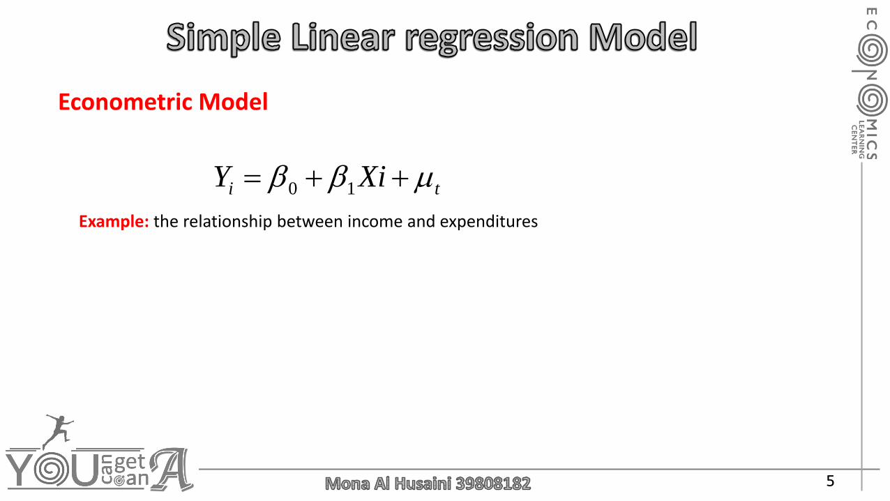
Econometric Model

Example: the relationship between income and expenditures

ti XiY ++= 10

6

Estimated Model

ii XY 10

+=

Now how we can get the values of estimated parameters?

7

Estimated Model

ii XY 10

+=

( )( )( )

−

−−=

21

XX

YYXX

i

ii

XY 10

−=

8

Example:

n 1 2 3 4 5 6 7 8

Absent 4 7 15 14 12 7 18 3

Grade 85 81 70 74 71 88 66 89

What is the DV and IV?

9

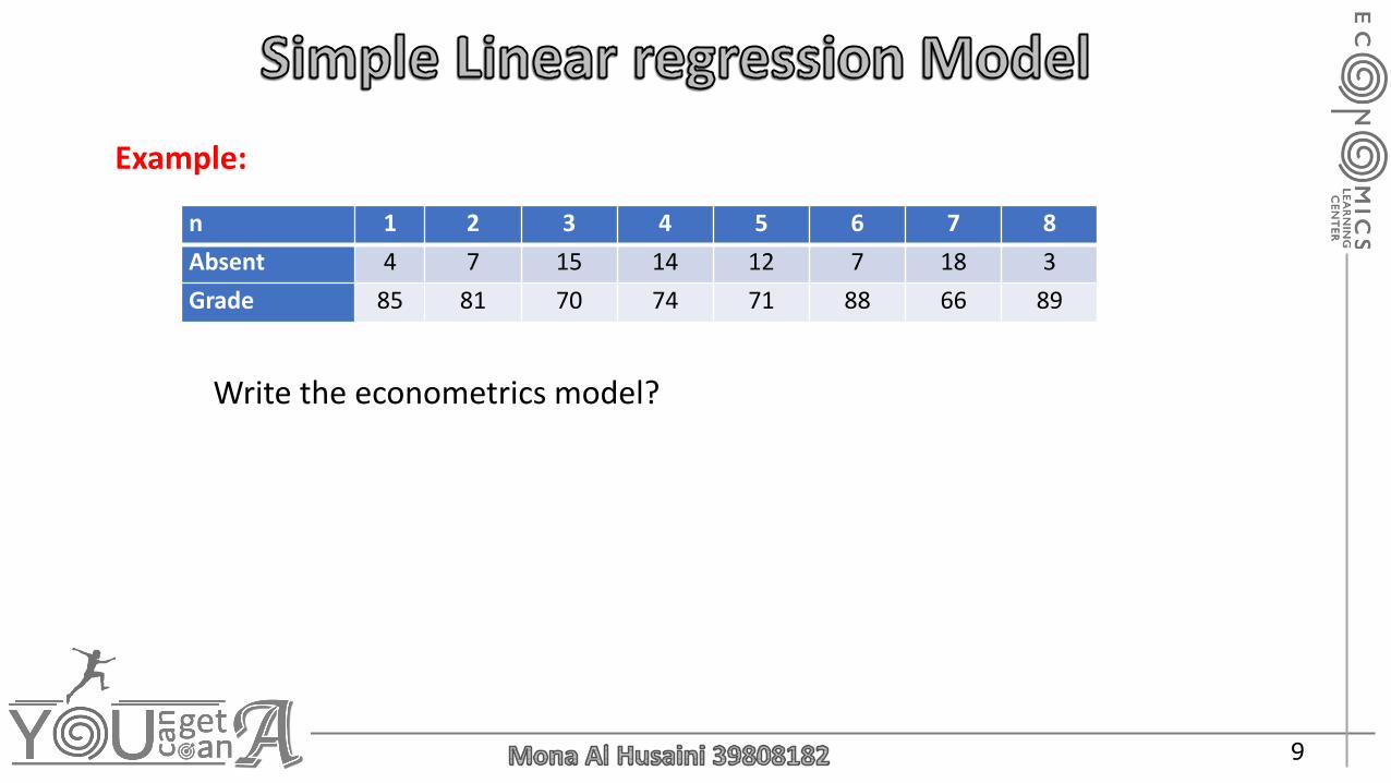
Example:

n 1 2 3 4 5 6 7 8

Absent 4 7 15 14 12 7 18 3

Grade 85 81 70 74 71 88 66 89

Write the econometrics model?

10

Example:

n 1 2 3 4 5 6 7 8

Absent 4 7 15 14 12 7 18 3

Grade 85 81 70 74 71 88 66 89

Write the estimated model?

11

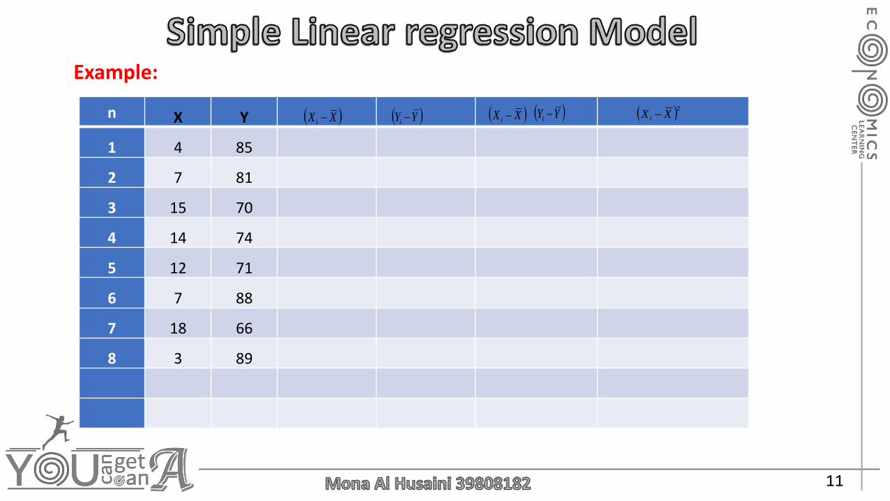
Example:

n X Y

1 4 85

2 7 81

3 15 70

4 14 74

5 12 71

6 7 88

7 18 66

8 3 89

( )XX i − ( )YYi −( )YYi −( )XX i − ( )2XX i −

12

Estimated Model

ii XY 10

+=

( )( )( )

−

−−=

21

XX

YYXX

i

ii

XY 10

−=

13

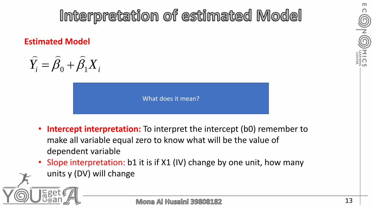
Estimated Model

ii XY 10

+=

What does it mean?

• Intercept interpretation: To interpret the intercept (b0) remember to make all variable equal zero to know what will be the value of dependent variable

• Slope interpretation: b1 it is if X1 (IV) change by one unit, how many units y (DV) will change

14

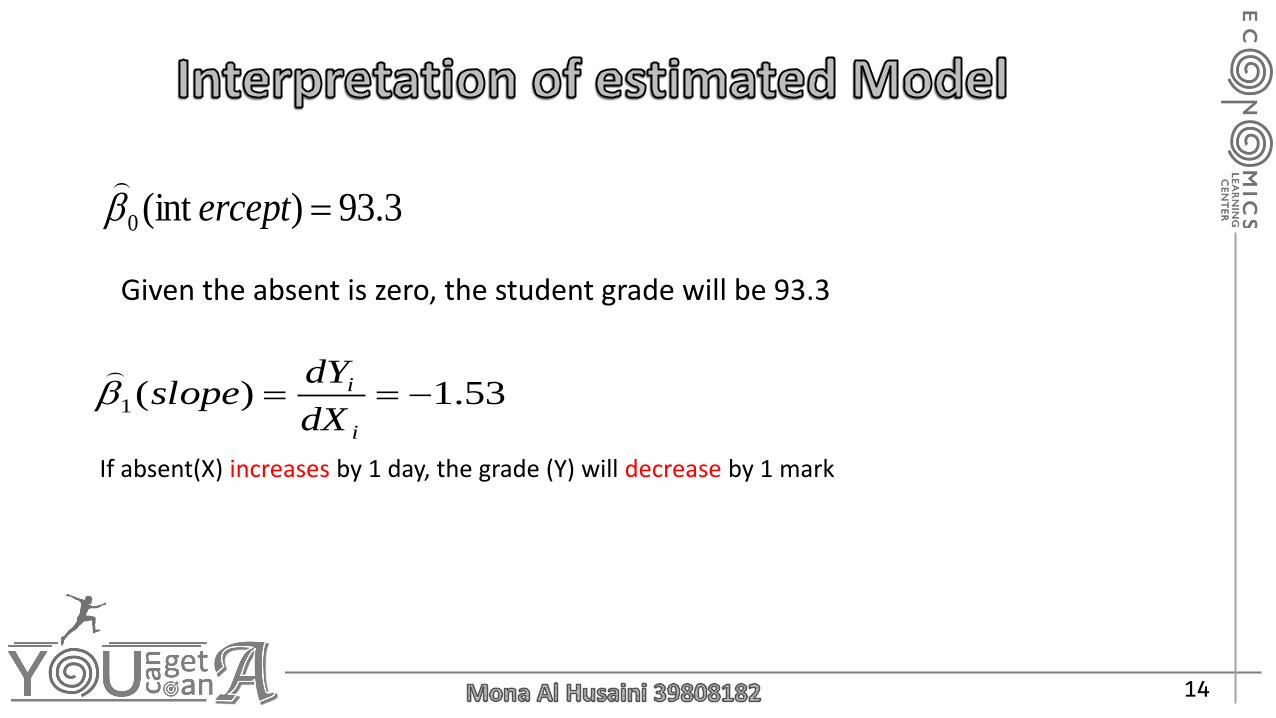
3.93)(int0 =ercept

Given the absent is zero, the student grade will be 93.3

53.1)(1 −==i

i

dX

dYslope

If absent(X) increases by 1 day, the grade (Y) will decrease by 1 mark

15

3.93)(int0 =ercept

53.1)(1 −==i

i

dX

dYslope

ii XY 10

+=

16

17

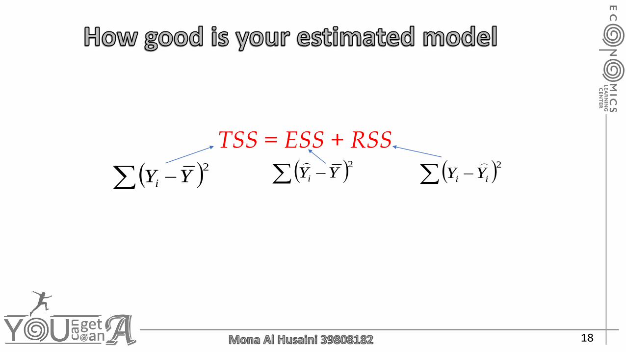
• How well the variations in dependent variable, Y is explained by the variations in

independent variable, X???

(A)total variation in Y

(A)total variations in Y explained by the model (i.e., independent variable, X)

(A)total variations in Y not-explained by the model (i.e., independent variable, X)

( )2 −YYi

( )2 −YYi

( )2 − ii YY

18

( )2 −YYi( )2 −YYi

( )2 − ii YY

TSS = ESS + RSS

19

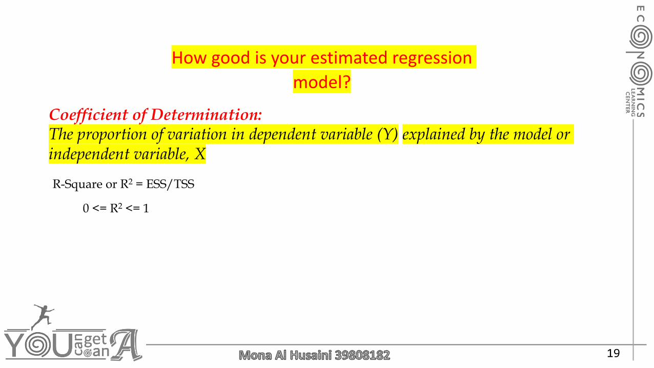
How good is your estimated regression

model?

Coefficient of Determination:The proportion of variation in dependent variable (Y) explained by the model or independent variable, X

R-Square or R2 = ESS/TSS

0 <= R2 <= 1

20

R2 = 0.897. what does it mean ?

89.7% variations in dependent variable, Y is explained by the independent variable, X (or, by the model)

If R2 = 0. what does it mean ?

If R2 = 1. what does it mean ?

21

• r is coefficient of the correlation. It shows the relationship between the two variables (positive or negative relationship. Whether there is strong or week relationship.

• -1 <= r <= +1

• r = 1 implies perfect correlation• r = 0 implies no correlation• Closer the value of r to 0, weaker is the relationship between X and Y• Closer is the value of r to 1, stronger is the relationship between X and Y

• R2: Coefficient of Determination: how the dependent variable is explained by the variation of independent variables• It measures the cause and effect relationship between two variables – X and Y, where X is the

cause factor and Y is the effect factor• The value is between 0 and 1• It tests the slope of the model

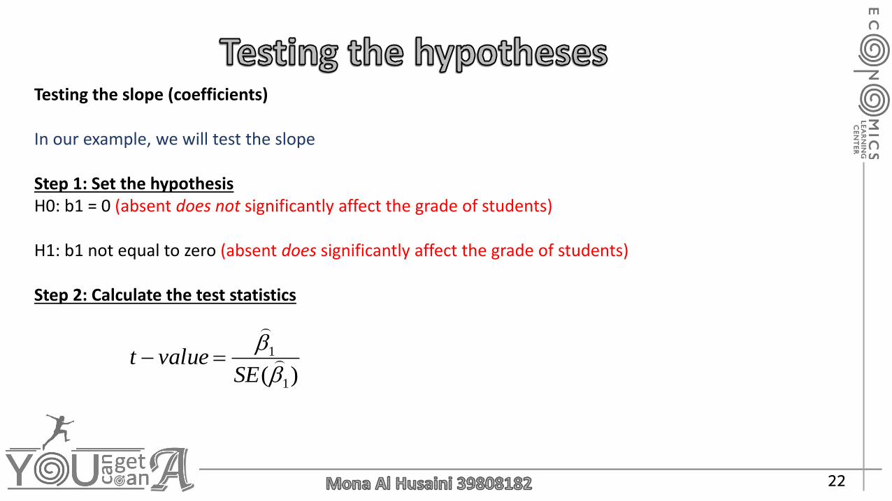
22

Testing the slope (coefficients)

In our example, we will test the slope

Step 1: Set the hypothesis H0: b1 = 0 (absent does not significantly affect the grade of students)

H1: b1 not equal to zero (absent does significantly affect the grade of students)

Step 2: Calculate the test statistics

)( 1

1

SEvaluet =−

23

21)(

1

)1()(

XXkn

RSSSE

i −

−−=

Degree of Freedom = n-k-1n = no of observationsk = no of independent variable

Se = 0.211

T- calculated = -1.5/0.211 = -7.2

24

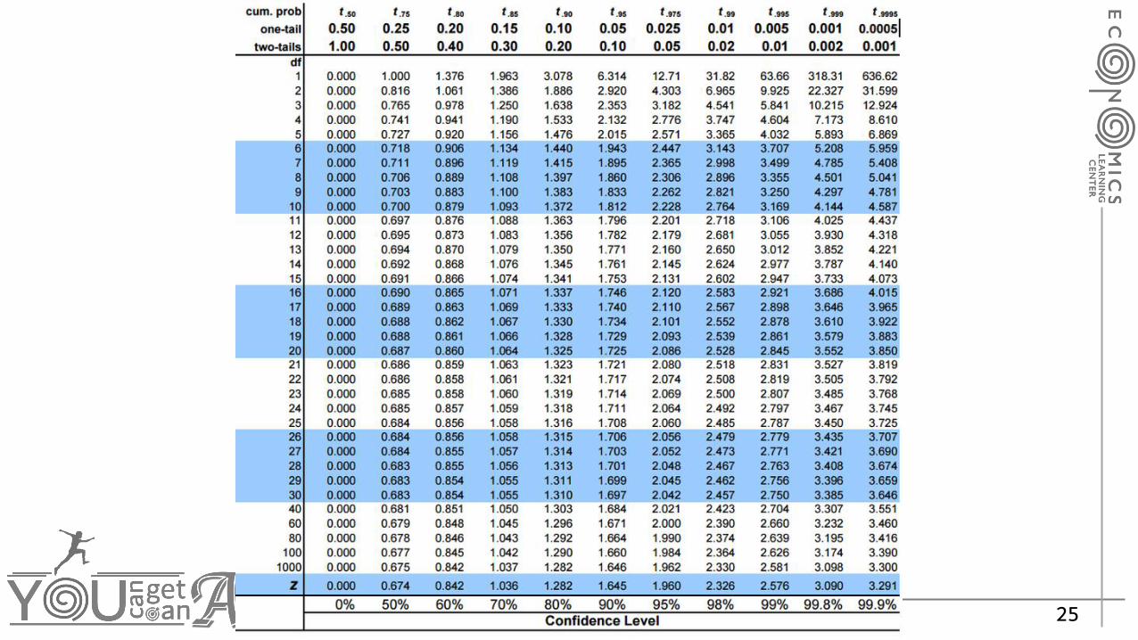
Step 3: find t-table (critical t-value)

• Which level of confidence:

Level of Confidence Level of Significance

99% 1% Alpha = 0.0195% 5% Alpha = 0.05

• What is the DoF

Degree of Freedom = n-k-1n = no of observationsk = no of independent variable

25

26

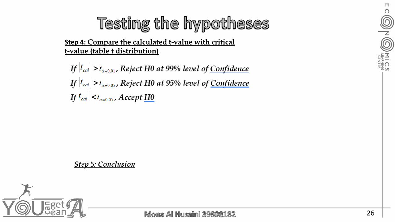
Step 4: Compare the calculated t-value with critical t-value (table t distribution)

Step 5: Conclusion

27

• This is the average of Y. You can calculate it by summing the valuesof Y and then dividing it by the number of the sample

Y

X • This is the average of X. You can calculate it by summing the valuesof X and then dividing it by the number of the sample

( )YYi − • The summation always equal 0

( )XX i − • The summation always equal 0

0= ie • This is the summation of the difference between actual Y andestimated Y

( ) 10

2, - unknowns respect to with

− ii YYMinimize