economic convergence. applications - second part

Institute of Economic Forecasting

Romanian Journal of Economic Forecasting – 4/2007 −

24

ECONOMIC CONVERGENCE. APPLICATIONS* - SECOND PART -

Aurel IANCU**

Abstract Real convergence is an essential objective of Romania’s integration into the EU. Bridging the development gaps between Romania and the EU as soon as possible cannot be achieved exclusively through market forces, since they rather tend to cause divergence and polarization. For this purpose, special tools and mechanisms are required; e.g., cohesion. The study deals with the economic convergence of the European countries, and especially the convergence of the CEE countries, including Romania. Models are used to assess the economic growth, approximate the period of real convergence of Romania to the EU, as well as to estimate the σ- and β-convergence, and the main shortcomings of the last indicator. Second part comprises some models and evidence of the economic growth and convergence.

Keywords: Real convergence, divergence, regression method, return to capital, σ-convergence, β-convergence. JEL Classification: C4, C5, F15, F43, F47, O41, O52, O57.

1. Evaluation of the opportunity to achieve a real convergence of Romania and the EU

For such evaluation it is necessary to point out Romania’s place among the EU countries and in the world by the GDP per capita. Second, we should define and evaluate Romania’s advance speed towards convergence with the developed countries or groups of countries, also taking into account the advancing speed of the developed countries or groups of countries.

* Study carried out within the project “Economic Growth, Employment and Competitiveness in

the Knowledge-based Economy”, CEEX 05-08 Programme No. 24/05.10.2005. ** Member of the Romanian Academy, and senior researcher at the National Institute of

Economics-Romanian Academy-Bucharest, e-mail: [email protected]

2

Economic convergence. applications

− Romanian Journal of Economic Forecasting – 4/2007

25

1.1. Romania’s place in the EU and the world by the growth

level and pace From an economic point of view, Romania is still in a marginal position if compared with the European developed countries. For example, if compared to the EU 25 average of 2004, Romania’s GDP per capita calculated by the exchange rate was 8.1 times lower, and that calculated by the purchasing power parity (PPP) was 3.1 times lower. If compared to the average of the ten countries 1 that acceded to the EU in 2004, Romania’s GDP per capita in 2004 was, according to the two calculation alternatives, 2.35 and 1.75 times lower2. Among the 28 member and candidate countries, in 2004, (EU27+Turkey), Romania is ranked the 26th (before Bulgaria and Turkey) by the GDP per capita calculated by PPP in euros. If we go beyond the European area when analysing Romania’s place by the average income per capita, we find out that this country holds a better position. Still, the gap between the extreme cases seems to be more dramatic than on the European level. Among the 208 countries and independent territories, Romania is placed by the GDP per capita calculated according to the two alternatives (the exchange rate and the PPP in US dollars) farther from the extreme levels, but above the average world level (Table 1).

Table 1 Romania’s relation to the EU 25 and EU 15 average level, the world’s

extreme levels and the world’s average GDP per capita in euros and US dollars, at the exchange rate and PPP, in 2004

GDP per capita calculated by the

exchange rate (EUR and USD)

GDP per capita calculated by the

PPP (EUR and USD)

Relation to the average EU 25 level > 8.1 times (lower) > 3.1 times (lower) Relation to the average EU 15 level > 9.1 times (lower) > 3.4 times (lower) Relation to the world’s average level < 1.3 times (higher) < 1.25 times

(higher) Relation to the world’s poorest country < 32.8 times (higher) < 15.1 times

(higher) Relation to the world’s richest country > 17.5 times (lower) > 4.8 times (lower) Source: Based on the World Bank’s data, 2006 World Development Indicators. To answer the question whether Romania succeeds to achieve convergence with the EU and the world’s top countries as regards the GDP per capita, we have to compare Romania’s progress and the progress made by the other countries or groups of countries. If we define the progress by the annual average growth rate of the GDP per

1 The group of ten countries include: Cyprus, Czech Republic, Estonia, Lithuania, Latvia, Malta,

Poland, Slovakia, Slovenia, Hungary. 2 Based on the Eurostat data.



26

capita* and analyse Romania’s rate in relation to other countries or groups of countries (Table 2) over as long periods of time as possible, we conclude that, in fact, Romania’s convergence is a mere illusion. Not only it is impossible to be achieved, but the gaps become broader, since (see the table) Romania’s annual average rate was much slower between 1990 and 2004 or even negative in the period 1980-2003.

Table 2 Annual average growth rate of the GDP per capita: comparison between

Romania and other developed countries and groups of countries (%)

1980-2003 1990-2004 2001 2000

2002 2001

2003 2002

2004 2003

Romania -0.6 1.3 6.2 5.5 5.5 8.7 Developed economies

2.1 1.9 0.7 0.7 1.5 1.9

EU 15 1.9 1.8 1.4 0.7 0.5 1.9 France 1.6 1.5 1.7 0.8 0.0 1.9 Germany 1.8 1.2 0.7 0.0 -0.2 1.5 USA 2.1 2.2 -0.2 0.9 2.1 3.2 Poland 1.8 4.1 1.1 1.4 3.9 5.4 Hungary 1.0 2.7 4.1 3.8 3.2 4.5 Source: UNCTAD, Handbook of Statistics, 2005. Although the analysis and forecast calculations require long series of data, we consider it is unreasonable to use for Romania the 1980-2000 data, since the two decades are non-typical as regards the economic continuity and stability. In that period Romania’s economy was in a profound and long crisis, when, on one hand, the centralized system showed (in the 1980’s) inefficiency and no capability to innovate and adapt and, on the other hand, the transition to a new system (in the 1990’s) consisted in a general profound restructuring of the entire economy (the technological and organizing system, the property system, the economic and social management, the institutions, etc.), which caused a major failure of the national economic system. The changes began to produce good results since 2000, when the stability and functioning of the economy were achieved on the basis of the new principles1. Therefore, we firmly support the idea that for the convergence scenarios and calculations one should consider, in the case of Romania, the growth rates from 2000 on, as they are significant and credible for the future evolution of Romania’s economy, when it began a normal development.

* GDP calculated on the basis of the PPP. 1 Once again M. Olson’s thesis that national economic systems naturally follow long life cycles

is confirmed. After a long functioning period, the institutions, the mechanisms and the social relations become rigid and do not respond to changes, which seriously affects the efficiency of the economic processes. The institutional restructuring offers the opportunity for changing the economic growth by adaptation and innovation (Mancur Olson, 1982, The Risk and Decline of Nations, Economic Growth Stagflation and Social Rigidities, Yale University Press, New Haven).



27

3.2. The assessment of the time required for convergence The most frequent question concerning the economic growth convergence refers to the length of the process. Specifically, when we analyse the convergence of the real economies of Romania and the EU, the first thing to be clarified is the length of the period necessary to achieve the future balance between Romania’s annual average income per capita (YR) and the EU15 one (YE). The initial level of the GDP per capita (expressed by the PPP in euros) of the two entities (YoR and YoE) is characterized by a significant difference. In 2004, the ratio of YOR to YOE was 1 : 3.4. The balance may occur in a reasonable period of time, only if Romania is able to achieve annual average growth rates per capita ( Rr ) much higher

than those achieved by the EU ( Er ), that is Rr > Er .

To assess the convergence period we start with the simple relations concerning the GDP per capita growth of the two entities with different initial levels and annual average growth rates:

tRORtR rYY )1( += (4)

tEOEtE rYY )1( += . (5)

The convergence is achieved when the values of the two relations become equal according to the relation (6):

YOR(1+ r R)t = YOE(1+ r E)t (6) And the curves YtR and YtE meet in the balance point t* (steady state), according to Figure 3:

Figure 3 The convergence of the economic growth curves of the developed

countries (YtE)

and the less developed countries (YtR) in the balance point t*



28

By logarithmating and rearranging the terms, one may assess the period of time (t) when the convergence (balance) of the GDP per capita of the two entities is achieved:

)1log()1log(

loglogER

OROE

rrYY

t+−+

−= (7)

Using this formula, we may calculate the period of time (in years) when Romania can catch up (as regards the GDP per capita calculated by the PPP in euros) with the EU 15 and two EU leaders: France and Germany. Catching up with the developed countries is achieved due to the higher growth rates in 2000-2004, namely when the restructuring effects occurred and the system began to function on the basis of the new principles and in the new external context. Table 3 includes the data used in the calculation formula (initial GDP per capita and the annual average growth rates) and the results representing the number of years required to achieve convergence with the EU 15, France (Fr) and Germany (Ge), in relation to Romania’s annual average growth rates, considered as alternatives ( r R1 = 4%; r R2 = 5%; r R3 = 6%; r R4 = 7%; %8r 5R = ), similar in size to the 2001-2004 ones.

Table 3 Forecasting the number of years to achieve the convergence of Romania

and the EU 15, France and Germany in relation to the GDP per capita calculated by the PPP in euros

Initial GDP per capita (2004)

Number of years(t) to achieve the convergence of alternative

annual average growth rates in Romania** ( 51..... RR rr )

UE 15 and leading countries (France and Germany)

Romania

Annual average growth rates of the EU 15 and EU countries

(France and Germany)*), 1990-2004

4% 5% 6% 7% 8%

YOUE = 24600 Y0R = 7300

r UE =1.8% 57 39 30 24 20

YOFr = 24800 Y0R = 7300

r Fr =1.5% 50 36 28 23 18

YOGe = 24600 Y0R = 7300

r Ge =1.2% 45 33 26 22 16

*) The annual average growth rates of the GDP per capita between 1990-2004. **) As regards Romania, the five rate alternatives (4%; 5%; 6%; 7%; 8%) are within the variation range of the same over the period 2000-2004. Source: Calculation based on Eurostat and UNCTAD data, Handbook of Statistics, 2005. According to the Table data, at an annual average growth rate of 4%, Romania would need 57 years to reach the EU 15 level, 50 years to reach France’s level, and 45 years to reach Germany’s level. At a growth rate of 7%, the number of years to achieve convergence would diminish to less than half, i.e., 24 years with EU 15, 23



29

years with France and 22 years with Germany, and at a rate of 8%, convergence requires 20 years with EU 15, 18 years with France and 16 years with Germany. The dynamics of the GDP per capita points of convergence of Romania and the EU 15 in relation to Romania’s average growth rates as against the EU rate is shown in Figure 4, where the abscissa contains the time (number of years) necessary to achieve the convergence, and the ordinate indicates the evolution of the GDP per capita in Romania, as given by the five alternatives of annual average rates.

Figure 4 The dynamics of convergence between Romania and the EU, in relation

to the GDP per capita by size of the annual average growth rates in Romania

Source: Own calculation on the 3 table and Eurostat data. At a 4 percent growth rate of Romania’s economy and the 1.8 percent one of the EU 15, the convergence point (curve intersection) of the two entities will be achieved at a GDP per capita of about 63200 euros, that is 57 years, and a rate of 8% for Romania and 1.8% for the EU 15, the convergence of the two entities will be achieved at a GDP per capita of about 34500 euros, that is 20 years.

3.3. The σ-convergence The measurement of convergence may be made by means of analytical tools and indicators, able to reveal the difference diminution (dispersion of the phenomenon) as against the average, or the gradual diminution in the difference between two or more time series: ayxt =−∞→ )(lim (8) The diminishing difference between the two variables is measured by either the stochastic principle or the non-stochastic one.



30

A frequently used indicator for the convergence measurement is the variation coefficient of the GDP per capita denoted by σ and calculated as follows:

t

n

ititt XXX

n/)(1

1

2∑=

−=σ (9)

This indicator is also known as σ-convergence1, first used by Sala-i-Martin, along with β-convergence. It may be used to characterize the convergence level by measuring the dispersion of the GDP per capita in a year, by means of the cross-section series (countries and regions). In this case, the relevance of the convergence indicator occurs only when comparisons are made. To characterize the convergence evolution (trend), time series (a discrete time interval, t and t+T) are used. When the phenomenon dispersion decreases over a period of time (when the indicator value diminishes over time), it means that convergence takes place, σt+T<σt, and when the dispersion increases, it means that divergence takes places, σt+T>σt. We used this indicator in our study to measure the level and evolution of the real convergence of the EU member countries by the three groups, EU 25, EU 15 and EU 102 - and the two GDP expressing alternatives: purchasing power parity and exchange rate. Due to the non-availability of data on some countries included in the panel (especially those which joined the EU recently), the time series was reduced to 12 years (1995-2006), of which the 2006 data are estimated. Table 4 includes the results of the calculations by the two modes of expression (PPP and exchange rate) and the three groups of countries, EU 25, EU 15 and EU 10 in relation to the σ-convergence indicator. The alternative calculated by the PPP in euros is presented graphically in Figure 5. To express visually the tendency of the phenomenon analytically, we present graphically (Figure 6) the primary data used to calculate the σ-convergence, namely, the evolution of the dispersion of the GDP per capita (expressed in PPP in euros) for 27 EU countries. The graph excludes Luxembourg and includes also Romania, Bulgarian and Turkey beginning with the years on which data expressed in PPP in euros (1999 for Romania) are available.

Table 4 The numerical evolution of the σ-convergence (the variation coefficient

of the GDP per capita), EU 25, EU 15 and EU 10 1 In their papers, Barro and Sala-i-Martin used for the measurement of the convergent σ

indicator the standard deviation calculated by the formula:

2

1 *log1

∑=

=⎥⎥⎦

⎤

⎢⎢⎣

⎡⎟⎟⎠

⎞⎜⎜⎝

⎛n

i y

iy

nσ ,

∑=

≡n

i iyn

y1log

1*log (Karl-Johan Dalgaard, Jacob Vastrup, “On the measurement of σ-

Convergence”, Economics Letters, 70 (2001) 283-287). Other authors use either the variation coefficient (e.g., Milton Friedman, Do Old Fallacies Ever Die, JEL, 30, 4, 1992), or both indicators.

2 It consists of the ten countries that joined the EU in 2004.



31

Calculated by PPP Calculated by exchange rate Years EU 25 EU 15 EU 10 EU 25 EU 15 EU 10

1995 0.44 0,25 ....... 0.71 0.38 ..... 1996 0.43 0.25 ....... 0.68 0.36 ..... 1997 0.42 0.23 ....... 0.65 0.33 ..... 1998 0.41 0.23 0.35 0.64 0.33 0.81 1999 0.44 0.27 0.36 0.66 0.35 0.86 2000 0.44 0.27 0.34 0.65 0.35 0.77 2001 0.42 0.26 0.33 0.63 0.34 0.67 2002 0.42 0.27 0.31 0.63 0.35 0.66 2003 0.43 0.29 0.28 0.63 0.36 0.69 2004 0.43 0.30 0.27 0.63 0.36 0.64 2005 0.42 0.32 0.24 0.62 0.37 0.55 2006x) 0.42 0.32 0.24 0.62 0.39 0.51 x) Estimated data. Source: Based on Eurostat data.

Figure 5

The σ-convergence (the variation coefficient) calculated by the GDP per capita (PPP in euros)

Source: Based on Eurostat data.



32

Figure 6 The evolution of the GDP per capita (PPP in euros) of the twenty-eight

EU member and applicant countries, 1990-2006

Source: Based on Eurostat data. Analysing the data from Table 4 concerning the numerical evolution of the σ-convergence, as well as the curves drawn in Figures 5 and 6, we may draw some important conclusions: 1. The evolution of the indicator concerning the variation coefficient of the GDP per

capita of the EU 15 countries (σ)shows some growth for both calculation alternatives (PPP and exchange rate), which means an ascending trend in the divergence of this group of economies.

2. As for the enlarged group, EU 25, we find a slight decrease in the variation coefficient for both calculation alternatives (PPP and exchange rate), that is, as a whole, a convergent growth owing to the EU 10 group.

3. There is a significant difference between EU 25 and EU 15 in the level of the variation coefficient of the GDP per capita calculated by the exchange rate, as against the level of the same indicator calculated by the PPP. It means that the less developed EU member countries, especially those that joined the EU in 2004, had and still have significantly underappreciated national currency, which strongly influence the high dispersion degree of the economies. The appreciation of the national currency along with the integration significantly diminishes the dispersion degree, calculated by the exchange rate, that is the diminution from 0.71 in 1995 to 0.62 in 2006 and, implicitly, in the difference between the two types of expression.



33

4. The evolution of the dispersion of the GDP per capita (Figure 6) for 27 countries

shows the formation, within the enlarged EU, of three groups of countries, each with specific features , but also the real opportunity for the less developed countrys to achieve higher development levels. Considering the growth rate in the last five years and the available resources, Romania is one of the most dynamic European economies, able to achieve the convergent growth.

3.4. The β-convergence Besides the σ indicator expressed by the variation coefficient or standard deviation, there were strong concerns to develop the methodological apparatus for the study of the convergence. Among them, it is worth mentioning the econometric research of various statistical cross-section or time series to reveal, by means of the regression equations and estimated trend, the convergence or divergence trend in the evolution of the economies in the world, EU and OECD. A major role in the econometric research is played by the estimation and interpretation of the β parameter of the regression equation of economic growth.

3.4.1. Conceptual and methodological aspects Although contested by some economists (Friedman, 1992; Quah, 1993) for being ire-levant for the real convergence of economic growth1, the concept of β-convergence plays a significant role in the literature. It is even indispensable as an econometric calculation and analysis tool for the description of this process when it is considered either in its simple initial form (absolute β-convergence) or the developed form (conditional β-convergence). The determination of the β-convergence indicator does not exclude or replace the σ-convergence indicator. They are linked or related and, as we shall see, they verify one another. If, according to the neoclassical theory of the decreasing rate of return on capital, we agree with the idea that poor economies tend to grow faster than rich ones, it means, on one hand, a gradual diminution in the dispersion coefficient of the GDP per capita (σt0+T<σt0) and, on the other hand, a reverse relation between the rate of the GDP per capita growth within a time interval (t0 and t0+T) and the initial level of the GDP per capita (year t0).

Tttiti

T

ti

Tti yTea

yy

T +

−+ +⎟⎟

⎠

⎞⎜⎜⎝

⎛ −−=⎟

⎟⎠

⎞⎜⎜⎝

⎛00

0

0,0, ,)log(1

,,

log1 εβ

(10)

1 Friedman points out that, according to the definition, the indicator of the β-convergence could

be replaced with the variation coefficient of the distribution of the GDP per capita among coun-tries/regions, that takes into account the inter-temporal changes in the GDP per capita among the countries. Quah shows that this indicator is subject to Galton’s failure. He stresses that the convergence analysis is just what the dynamics of the income distribution reveals. Quah’s convergence test, using Markov’s chain for the intertemporal transition model of the income distribution, could control the dynamics of the entire distribution of the income of all countries. Friedman and Quah show that the regression model could wrongly indicate the presence and expansion of the β-convergence (G.E. Boyle and T.G. McCarthy, “A Simple Measure of β-Convergence”, Oxford Bulletin of Economics and Statistics, 59, 2 (1997), p. 257-258).



34

This relation is a theoretical hypothesis that is to be econometrically tested on the basis of the statistical data on a representative sample of countries. The tendency of the poor countries to catch up with the rich ones is reflected both by the diminution in the dispersion degree of the GDP per capita among the countries and by the negative sign of the annual rate of β-convergence of the GDP per capita of the sampled countries, as they reach the steady state1 at the same time. Following the testing, between the two indicators, σ and β, the following three combinations (C) may occur during period T:

C1 C2 C3

00 tTt σσ <+ (convergence)

00 tTt σσ >+ (divergence)

00 tTt σσ<

+ >

(divergence, standstill, convergence)

- β (convergence) + β (divergence) ± β (divergence or convergence)

Decreasing distance between the development levels of the economies in period T

Increasing distance between the development levels of the economies in period T

Within period T, the decrease and increase in the distance between the development levels of the economies may take place successively

In the case of the combination C3 within the period T, oscillations or even reversals of the levels of the GDP per capita may occur in relation to the poor (S) and rich countries (B) included in the panel (Figure 7).

Figure 7 Possible evolution of the GDP per capita of the poor countries (S) in

relation to the rich ones (B) in period T

1 The negative sign of the β parameter is the expression of the reverse relation between the

annual average growth rate of the GDP per capita over the period T and the initial level of the GDP per capita in the year t0.



35

Considering the above-mentioned comments on the relations between the σ and β indicators, we may conclude: 1) A necessary condition for convergence is the existence of the β-convergence; 2) Although necessary, the β-convergence is not a sufficient condition for the σ-convergence. The β indicator, estimated by the regression equation, expresses the rate of convergence of the countries towards the steady state. It considers the income mobility within the same distribution (dispersion) which is considered by the σ-convergence in relation to their evolution over time1. The concept of β-convergence, generated by the analysis of the regression of the development level of the countries/regions, may take three basic forms, depending upon the depth of the analysis and the degree of compliance with the economic realities within the range allowed by the neoclassical model of convergent growth: 1) absolute β-convergence; 2) β-convergence clubs; 3) conditional β-convergence. Briefly speaking, these forms consist of the following: 1. The absolute β-convergence is the alternative that only takes into account the

assumption of the high growth rates of the poor countries as against the rich ones, irrespective of the differentiated evolution of the sample countries regarding the determinants of growth over the entire period of time (T) of the data used for the regression calculation. Since in this period of time there are significant technological, institutional, behavioural discrepancies between countries/regions that affect the results, it is necessary to find those solutions that are based on realities, but not exceeding the limits of the neoclassical methodological area.

2. The easiest solution is the β-convergence clubs, which include in the studied panel the countries/regions that show some technological, institutional and economic policy homogeneity, etc. The key assumption accepted for this solution requires that the same group should not show significant initial differences among the countries/regions of the club as regards the GDP.

3. Another solution is the conditional β-convergence, that takes into account the vector of the determinants of the growth as additional variables that define the differences among the economies that stand proxy for the achievement of the steady state by introducing in the regression equation some variables that keep a constant balance of the economies.

Further, we try to test the first two forms of convergence. The third form, the conditional β-convergence, will be discussed in a separate study. Since the neoclassical model of convergence, on which the (especially, absolute) β-convergence is based, takes into account the assumption concerning the decreasing rate of return to capital, in the final part of our study we try to test this hypothesis by calculating the relation between the investment rate of return and the countries’ development level. It is an important scientific factor that requires the testing of this key hypothesis validity in the present economic realities, to see to what extent we may count on the neoclassical model of the absolute (non-conditional) β-convergence and why the model should be reviewed or modified. 1 Xavier Sala-i-Martin, “Regional Cohesion: Evidence and Theories of Regional Growth and

Convergence”, European Economic Review, 40 (1996), p. 1326; G.E. Boyle and T.G. McCarthy, op. cit., p. 258.



36

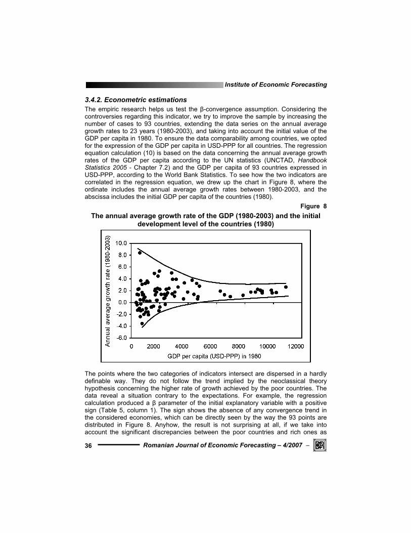
3.4.2. Econometric estimations The empiric research helps us test the β-convergence assumption. Considering the controversies regarding this indicator, we try to improve the sample by increasing the number of cases to 93 countries, extending the data series on the annual average growth rates to 23 years (1980-2003), and taking into account the initial value of the GDP per capita in 1980. To ensure the data comparability among countries, we opted for the expression of the GDP per capita in USD-PPP for all countries. The regression equation calculation (10) is based on the data concerning the annual average growth rates of the GDP per capita according to the UN statistics (UNCTAD, Handbook Statistics 2005 - Chapter 7.2) and the GDP per capita of 93 countries expressed in USD-PPP, according to the World Bank Statistics. To see how the two indicators are correlated in the regression equation, we drew up the chart in Figure 8, where the ordinate includes the annual average growth rates between 1980-2003, and the abscissa includes the initial GDP per capita of the countries (1980).

Figure 8 The annual average growth rate of the GDP (1980-2003) and the initial

development level of the countries (1980)

The points where the two categories of indicators intersect are dispersed in a hardly definable way. They do not follow the trend implied by the neoclassical theory hypothesis concerning the higher rate of growth achieved by the poor countries. The data reveal a situation contrary to the expectations. For example, the regression calculation produced a β parameter of the initial explanatory variable with a positive sign (Table 5, column 1). The sign shows the absence of any convergence trend in the considered economies, which can be directly seen by the way the 93 points are distributed in Figure 8. Anyhow, the result is not surprising at all, if we take into account the significant discrepancies between the poor countries and rich ones as



37

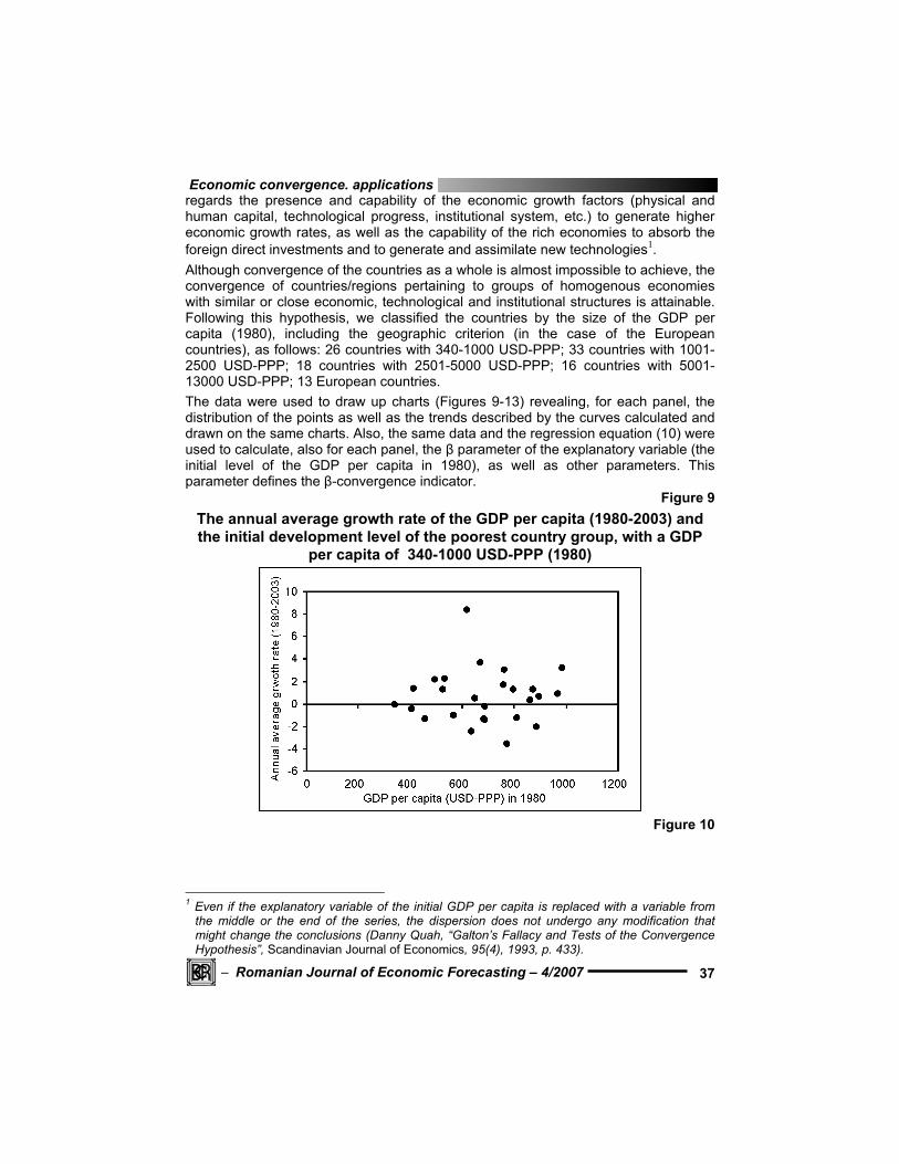
regards the presence and capability of the economic growth factors (physical and human capital, technological progress, institutional system, etc.) to generate higher economic growth rates, as well as the capability of the rich economies to absorb the foreign direct investments and to generate and assimilate new technologies1. Although convergence of the countries as a whole is almost impossible to achieve, the convergence of countries/regions pertaining to groups of homogenous economies with similar or close economic, technological and institutional structures is attainable. Following this hypothesis, we classified the countries by the size of the GDP per capita (1980), including the geographic criterion (in the case of the European countries), as follows: 26 countries with 340-1000 USD-PPP; 33 countries with 1001-2500 USD-PPP; 18 countries with 2501-5000 USD-PPP; 16 countries with 5001-13000 USD-PPP; 13 European countries. The data were used to draw up charts (Figures 9-13) revealing, for each panel, the distribution of the points as well as the trends described by the curves calculated and drawn on the same charts. Also, the same data and the regression equation (10) were used to calculate, also for each panel, the β parameter of the explanatory variable (the initial level of the GDP per capita in 1980), as well as other parameters. This parameter defines the β-convergence indicator.

Figure 9 The annual average growth rate of the GDP per capita (1980-2003) and the initial development level of the poorest country group, with a GDP

per capita of 340-1000 USD-PPP (1980)

Figure 10

1 Even if the explanatory variable of the initial GDP per capita is replaced with a variable from

the middle or the end of the series, the dispersion does not undergo any modification that might change the conclusions (Danny Quah, “Galton’s Fallacy and Tests of the Convergence Hypothesis”, Scandinavian Journal of Economics, 95(4), 1993, p. 433).



38

The annual average growth rate of the GDP per capita (1980-2003) and the initial development level of the group of countries with a GDP per

capita of 1001-2500 USD-PPP per capita (1980)

Figure 11 The annual average growth rate of the GDP per capita (1980-2003) and

the initial development level of the country group with a GDP per capita of 2501-5000 USD-PPP (1980)

Figure 12



39

The annual average growth rate of the GDP per capita (1980-2003) and

the initial development level of the country group with a GDP per capita of 5001-13000 (USD-PPP) (1980)

Figure 13 The annual average growth rate of the GDP per capita (1980-2003) and

the initial development level of some European countries (EU members, Norway and Turkey) (1980)

The β indicator as well as other estimated parameters are included in Table 5.



40

Table 5 The results of the regression calculation for all countries and groups of

countries of which:

Parameters Total 93 countries

26 countries, 340-1000 USD-PPP per capita



16 countries 5001-13000 USD-PPP per capita

13 European countries

A 1 2 3 4 5 6 β 0.584 0.256 1.876 -1.184 1.184 -0.548

Constant -3.127 -1.002 -12.915 12.031 -8.985 6.925 R² 0.084 0.001 0.068 0.040 0.302 0.146 r 0.289 0.030 0.261 0.199 0.549 0.382

t for β 2.852 0.148 1.458 -0.813 2.459 -1.373 St. Dev. 1.838 2.456 1.929 1.299 0.349 0.638

Source: Calculations based on data from the sources above mentioned. Out of all six panels calculated and introduced in the table, only those referring to the group of European countries (column 6) and the country group with an initial GDP per capita of 2501-5000 USD-PPP (column 4) have a negative β parameter. The other four panels have a positive β parameter, which proves a divergent trend.

2. The rate of return to capital and the question of convergence

The regression calculation made above did not confirm the automatic convergence even in the panel case by virtue of the theoretical assumptions, according to which the less developed countries would reach in a natural way the more developed ones. In the previous section, we found out that, following the econometric testing, the hypothesis concerning the β-convergence was not confirmed in most cases, when the same panel included the less and the more developed countries together. The first question to be answered in relation to the cause of the lack of convergence is whether the hypothesis of the decreasing rate of return to investment is confirmed. That is why we intend to test below the veracity of the assumption concerning the existence, under the present conditions, of the decreasing rate of return to capital or, in other words, the existence of the correlation between the rate of return to capital (investment in physical capital) and the countries’ development level (per capita GDP). There are two categories of indicators for testing the world trend:

• ∆ GDP, representing the per capita GDP growth in 2004 as against the previous year (2003), expressed in USD-PPP.

• The value of the investments in physical capital, per capita in 2003.



41

To ensure the calculation accuracy, the investment indicator has two alternatives dependent on the scope, namely:

• gross investment per capita resulted from saving (from accumulation and depreciation*);

• total investment per capita, consisting of gross investment to which the investment in physical capital from the international aid, investment from structural (solidarity) funds and FDI inflows should be added.

As investments produce effects with some delay, for the series of the two indicators – investment and production – a lag of one year, between 2003 and 2004, was considered. The rate of return to the gross investment (RRGI) is defined as the per capita GDP increase per one physical capital growth unit (per one monetary unit of gross investment): RRGI = ∆ GDP per capita/gross investment per capita To test econometrically the hypothesis concerning the descending trend of the rate of return along with the economic growth, we correlated the data regarding the indicator of the rate of return to the gross investment with the data regarding the indicator of the GDP per capita for a larger number of countries (Annex 2). The data concerning the two indicators specified in the above annex were used to draw up six charts, where the abscissa includes the GDP per capita (USD-PPP) of the countries in 2003, and the ordinate includes the rate of return of the gross investment calculated by the ratio of the GDP per capita in 2004 as against 2003 to the gross investment per capita from internal sources (accumulation and depreciation) in 2003 (RRGI). To see to what extent the rate of return trend could be influenced by the specific policies and institutions of the countries, we drew up charts of the groups of countries selected by the level of the GDP per capita and geographical criteria:

• A chart including all 180 countries on the UNO’s and World Bank’s records (Figure 14);

• Four charts of the countries grouped by the GDP per capita (Figures 15-18); • Two charts of the European countries (Figure 19) and the EU member countries

(Figure 20).

* This indicator corresponds to the notion of gross capital formation.



42

Figure 14 The rate of return to the gross investment (RRGI) by the development

level of the economies

Figure 15 The rate of return to the gross investment (RRGI) of the countries with a

GDP per capita of 550-2500 USD-PPP



43







44


GDP per capita of 15001- 40000 USD-PPP

Figure 19 The rate of return to the gross investment (RRGI) of the European

countries



45

Figure 20

The rate of return to the gross investment (RRGI) of the EU member countries

Each graphic includes also the estimated parameters of the simple regression equations. The graphical presentation and estimated parameters do not confirm for all panels the decreasing rate of return hypothesis. As for the European countries, with a slight decreasing trend of the return, the results should be viewed with a certain caution, since the less developed countries of this group, in 2003-2004, enjoyed an economic boom (high growth rates) after a deep recession. The trend in the rate of return to the gross investment of the groups of countries with a higher GDP per capita (Figures 16-18) is ascendant, which, on the one hand, contradicts the old hypothesis of the neoclassical theory and, on the other hand, confirms the new hypothesis of the endogenous theory according to which the effects of the technological progress and human capital are stronger. Therefore, Romer (1986) and Lucas (1988)were right in their argumentation. In the real economic life of the countries, the investments are not limited to the internal resources. There are also investments from foreign sources, such as the aid as investment in the physical capital granted to the poor countries by international organisations, investments in the solidarity or/and structural funds, as well as the FDI inflows received, in principle, by all countries, but, practically, in larger amount by the countries that offer comparative economic opportunities to investors and institutional, economic and political stability. To see the extent to which these categories of investments influence in a way or other the above rate of return to capital trend, we considered the contribution of all investments from the two (internal and foreign) sources. On the basis of all investments, we calculated a new more comprehensive indicator called the rate of return to the total investment (RRTI). This indicator, as an independent variable, is correlated with the development level of the countries (expressed as GDP per capita), as a dependent variable.



46

To compare the results obtained by the two ways of expressing the rate of return to capital, we drew up tables of the data series and the related charts, including all 180 countries and the groups of countries classified by the size of the GDP per capita and, separately, the European countries and the EU member countries. The charts are based on the data from the above mentioned sources. The results obtained by the rate of return to the total investment (RRTI) do not change significantly the results based on the above rate of return to the gross investment (RRGI), excepting EU member countries (see figures 11-20 and 26-27).

3. Conclusions Both the unconditional β-convergence and the decreasing returns to the physical capital are hypotheses concerning different growth rates, higher in the poor countries and lower in the rich ones, which ensure the proximity of the two categories of countries to one another and their joint transition to the steady state. Both hypotheses pertain to the neoclassical model that postulates the joint achievement of the convergence by the competitive market tools and places the investment in physical capital at the centre of the convergent economic growth. What one should note is that the initial differences among countries refer not only to the GDP per capita and the physical capital stock, specified above but also to the human capital and especially to its quality, to the scientific and technological stock, as well as the institutional and cultural frameworks, and their evolution according to the theory, there are no differences between countries. Properly, the study of convergence should consider the differences in the factors that, on one hand, require special costly investment that only a small number of countries (especially, the rich ones) may afford and, on the other hand, may cause stronger effects than the additional stock of physical capital may do. Moreover, one should also consider that, along with the market liberalisation and globalisation, there is an increasing mobility of the production factors (investment flows, scientific and technological competence, etc.) and, at the same time, their contribution to the economic growth increases, especially in the countries that have a higher economic, scientific and technological potential, are actively included in these international flows and take advantage of them. In the EU case there is an explicit policy and practical actions to achieve real economic convergence by means of the cohesion funds set up for the member and applicant countries less developed and the structural funds for the elimination of the disparities among the EU regions. The effects of the cohesion policy of the EU are pointed out by the trends in Figures 19-20 and Figures 26-27 and partially by the β indicator. As against the new general processes, the model of the unconditional β-convergence is not quite relevant, since the new requirements for the application of the model do not entirely cope with the above realities. Therefore, suitable convergence models are required to cope with the new realities.



47

Bibliography

1. ABRAMOVITZ M., 1986, Catching Up, Forging Ahead, and Falling Behind, "The Journal of Economic History”, vol. 46, No. 2, “The Tasks of Economic History” (June), 385-406.

2. AGHION PILIPPE, EVE CAROLI, CECILIA GARCIA-PENALOSA, 1999, Inequality and Economic Growth: The Perspective of the New Growth Theories, “Journal of Economic Literature”, vol. 37, No. 4 (Dec.), 1615-1660.

3. AHSAN SYED M., MELANIA NICA, 2005, Growth, Integration and Institutions in Eastern Europe and Former Soviet Union (EEFSU), Concordia University, April.

4. BARRO ROBERT J., XAVIER SALA-I-MARTIN, 1992, Convergence, Topic 2 “Dynamics and Convergence”, JPE, April.

5. BARRO ROBERT J., 1991, Economic Growth in a Cross-Section of Countries, “The Quarterly Journal of Economics” vol. 106, No. 2, May, 407-443.

6. BARRO ROBERT J., XAVIER SALA-I-MARTIN, BLANCHARD OLIVER JEAN, HALL ROBERT E., (1991), Convergence across States and Regions, “Brooking Papers on Economic Activity”, vol. 1991, No. 1, 107-182.

7. BARRO ROBERT J., XAVIER SALA-I-MARTIN, 1992, Convergence, “The Journal of Political Economy”, vol. 100, No. 2 (April), 223-251.

8. BARRO ROBERT J., XAVIER SALA-I-MARTIN, 1995, Economic Growth, The MIT Press, Cambridge Mass.,.

9. BASSANINI ANDREA, STEFANO SCARPETA, 2001/II, The Driving Forces of Economic Growth: Panel Data Evidence for the OECD Countries, “OECD Economic Studies”, No. 33.

10. CAMPOS NAURO F., CORICELLI FABRIZIO, 2002, Growth in Transition: What We Know, What We Don’t, and What We Should, “Journal of Economic Literature”, vol. XL (September), pp. 793-836.

11. CASTRO VILLAVERDE JOSÉ, 2004, Indicators of Real Economic Convergence. A Primer, United Nations University, UNU-CRIS E-WORKING PAPERS, w/2

12. COLLINS M. SUSAN, BARRY BOSWORTH P., 1996, Economic Growth in East Asia: Accumulation versus Assimilation, in vol. “Economic Development and Growth Papers, Brooking Papers Economic Activity”, No. 1.

13. DALGAARD CARL-JOHAN, JACOB VASTRUP, (2001), On the Measurement of σ-Convergence, “Economics Letters”, 70, 283-287.

14. DĂIANU DAN, 2003, Convergenţa economică. Cerinţe şi posibilităţi, în Aurel Iancu (coorodonator), “Dezvoltarea economică a României. Competitivitatea şi integrarea în Uniunea Europeană”, Editura Academiei Române, Bucureşti.

15. DOBRESCU EMILIAN, 2004, coord., Seminarul de modelare macroeconomică, Centrul de Informare şi Documentare Economică, mai.

16. HALL ROBERT E., JONES CHARLES I., 1999, Why Do Some Countries Produce So Much More Output per Worker than Others?, “The Quarterly Journal of Economics”, vol. 114, No. 1 (February), 83-116.

17. HAUSMANN RICARDO, PRITCHETT LANT, RODRIK DANI, 2004, Growth Accelerations, National Bureau of Economic Research, June.

18. HAVRYLYSHYN OLEH, 2001, Recovery and Growth in Transition: A Decade of Evidence, “IMF Staff Papers”.

19. IANCU AUREL, 1974, Modele de creştere economică şi de optimizare a corelaţiei dintre acumulare şi consum, Editura Academiei Române.

20. KANG SUNG JIN, 2002, Relative Backwardness and Technology Catching Up with Scale Effects, “Journal of Evolutionary Economics”, Springer Verlag.

21. KUTAN ALI M., TANER M. YIGIT, 2003, Convergence of Candidate Countries to the European Union.



48

22. LEE KEVIN, HASHEM PESARAN, RON SMITH, 1997, Growth and Convergence in a Multi-Country Empirical Stochastic Solow Model, “Journal of Applied Econometrics”, vol. 12, No. 4 (June-August), 357-392.

23. LUCAS ROBERT E. Jr., 1988, On the Mechanics of Economic Development, (în vol. “Economic Development and Growth Papers”), “Journal of Monetary Economics”, 22, 3-42.

24. LUCAS ROBERT E. Jr., 1990, Why Doesn’t Capital Flow from Rich to Poor Countries, “American Economic Review”, vol. 8.

25. MANKIW GREGORY, DAVID ROMER, DAVID N. WEIL, A Contribution to the Empirics of Economic Growth, “The Quaterly Journal of Economics”, vol. 107, No. 2, May 1992, 407-437.

26. MATKOWSKI ZBIGNIEW, MARIUSZ PROCHNIAK, Economic Convergence in the EU Accession Countries, Warsaw School of Economics, Internet.

27. MEEUSEN WIM, JOSÉ VILLAVERDE (Ed.), 2002, Convergence Issues in the European Union, Edward Elgar, UK.

28. MEIJERS HUUB, HOLLANDERS HUGO, 2001, Investments in Intangibles, ICT-Hardware Productivity Growth and Organisational Change: An Introduction, September.

29. MEYER DIETMAR, Creativity, Human Capital, and Economic Growth, “Society and Economy”, vol. XXI, No. 4, 1-8.

30. MIHĂESCU FLAVIUS, 2003, Convergenţa între economiile central şi est-europene, în Daniel Dăianu şi Mugur Isărescu (coordinators), “Noii economişti despre tranziţia în România”, colecţia Bibliotecii Băncii Naţionale, Bucureşti.

31. O’CONNOR JULIA S., 2005, Dimensions of Socio-Economic Convergence in the European Union: Convergence of What?, May 9.

32. OECD, 2001/II, OECD Economic Studies, No. 33. 33. PUGA DIEGO, 1998, The Rise and Fall of Regional Inequalities, Centre for Economic

Performance, “Discussion Paper”, No. 314, November 1996, Revised January. 34. ROMER PAUL M., 1986, Increasing Returns and Long-Run Growth, “The Journal of Political

Economy”, vol. 94, No. 5, (October), 1002-1039. 35. SALA-I-MARTIN XAVIER, (1996), Regional Cohesion: Evidence and Theories of Regional

Growth and Convergence, “European Economic Review”, 40, 1325-1352. 36. SALA-I- MARTIN, XAVIER, 1996, A Classical Approach to Convergence Analysis, “The

Economic Journal”, vol. 106, No. 437 (July), 1019-1036. 37. TEMPLE JONATHAN, 1999, The New Growth Evidence, “Journal of Economic Literature”

vol. 37, No. 1 (May), 112-156. 38. THIRLWALL A.P., 2001, Growth and Development with Special Reference to Developing

Economies (sixth ed.). 39. TORSTEN PERSSON, GUIDO TABELLINI, 1994, Is Inequality Harmful for Growth?, The

American Economic Review, vol. 84, No. 3, (June), 600-621. 40. WARWICK J. Mc KIBBIN, 1998, Forecasting the World Economy Using Dynamic

Intertemporal General Equilibrium Multi-Country Models, 22 September. 41. ZIPFEL JACOB, 2004, Determinants of Economic Growth, Florida State University.

economic convergence. applications - second part

Documents