Upjohn Institute Technical Reports Upjohn Research home page

1-1-1993

Economic Development and Black Economic Success Economic Development and Black Economic Success

Timothy J. Bartik W.E. Upjohn Institute for Employment Research, bartik@upjohn.org

Upjohn Author(s) ORCID Identifier:

https://orcid.org/0000-0002-6238-8181

Follow this and additional works at: https://research.upjohn.org/up_technicalreports

Part of the Regional Economics Commons, and the Social Policy Commons

Citation Citation Bartik, Timothy J. 1993. "Economic Development and Black Economic Success." Upjohn Institute Technical Report No. 93-001. Kalamazoo, MI: W.E. Upjohn Institute for Employment Research. https://doi.org/10.17848/tr93-001

This title is brought to you by the Upjohn Institute. For more information, please contact repository@upjohn.org.

ECONOMIC DEVELOPMENT

AND BLACK ECONOMIC SUCCESS

Upjohn Institute Technical Report No. 93-001

Timothy J. Bartik Senior Economist

W. E. Upjohn Institute for Employment Research300 South Westnedge Avenue

Kalamazoo, MI 49007

Final Report prepared for

U.S. Department of CommerceEconomic Development Administration

Technical Assistance and Research Division

January, 1993

The statements, findings, conclusions, and recommendations in this report are those of the author and do not necessarily reflect the views of the Economic Development Administration.

ECONOMIC DEVELOPMENT AND BLACK ECONOMIC SUCCESS

Timothy J. Bartik Senior Economist

W. E. Upjohn Institute for Employment Research300 South Westnedge Avenue

Kalamazoo, MI 49007

Final Report prepared for

U.S. Department of CommerceEconomic Development Administration

Technical Assistance and Research Division

January, 1993

BetelU.S. DEPARTMENT OF COMMERCEECONOMIC DEVELOPMENT ADMINISTRATION

ECONOMIC DEVELOPMENT AND BLACK ECONOMIC SUCCESS

Timothy J. Bartik Senior Economist

W. E. Upjohn Institute for Employment Research300 South Westnedge Avenue

Kalamazoo, MI 49007

Final Report prepared for

U.S. Department of CommerceEconomic Development Administration

Technical Assistance and Research Division

January, 1993

The statements, findings, conclusions, and recommendations in this report are those of the author and do not necessarily reflect the views of the Economic Development Administration.

Contents

Page

ACKNOWLEDGEMENTS ...................................... vii

ABSTRACT .............................................. .viii

EXECUTIVE SUMMARY ...................................... ix

I. Introduction ........................................... 1

Increasing Income Inequality and Shifts in Labor Skill Demand and Supply .... 2The Spatial and Skills Mismatch View ........................... 3Metropolitan Growth and Decentralization ......................... 5The Capitalization Hypothesis ................................ 6The Implications of Hysteresis Effects and Efficiency Wage Effects ......... 8Outline of the Rest of This Report ............................. 9

II. Review of Previous Research Related to Local Economic Development andBlack Economic Success ................................... 9

General Studies of Local Growth and Average Economic Outcomes ......... 10The Relationship of Black Economic Outcomes to the Overall Local Economy

and the Local Industrial Mix ............................ 10The Spatial Mismatch Literature: Effects of Job Access on Black Economic

Outcomes ........................................ 18

III. Methodology and Data ..................................... 19

Specification of the Estimating Equations ......................... 20Dependent Variables ...................................... 23Independent Variables ..................................... 27The Direction of Causation Issue .............................. 35

IV. Preliminary Analysis of Trends in Dependent and Independent Variables ...... 36

National Trends in "Regression-Adjusted" Personal Earnings for Large MSAs . . 36 Differences in Economic Trends Across MSAs ...................... 39National Trends in Economic Development Variables .................. 43Variations in Economic Development Trends Across MSAs .............. 47

Contents(Continued)

V. Effects of MSA Growth on Black and White Economic Success ........... 54

Estimated Long-Run Effects of MSA Growth on Black and White PersonalEarnings ......................................... 58

Consequences for Poverty Rates of Growth's Effects on Personal Earnings.............................................. 63

Effects of Growth on the Earnings of Various Subgroups of Blacks and Whites . . 65 Effects of Evening Out Growth ............................... 69

VI. Effects of Changes in MSA Industrial Mix on Black and White EconomicSuccess .............................................. 71

Strategy for Estimating the Effects of MSA Industrial Mix ............... 71Effects of Alternative Measures of Industrial Mix on Real Personal Earnings . . 73 Further Exploration of the Effects of the MSA Industry Wage Premium on

Personal Earnings ................................... 82

VII. Effects of MSA Decentralization on Black and White Economic Success ...... 89

VIII. Conclusion ............................................ 93

REFERENCES ............................................. 96

TECHNICAL APPENDIX ..................................... T-1

Details on the Estimation Methodology ......................... T-1Details on the Regression-Adjusted Economic Outcome Variables ......... T-12Details on the Construction and Use of the Economic Development Variables . . T-26

11

List of Tables

Page

Table 1 Summary of Previous Research on Black Economic Outcomes, OverallLocal Economic Strength, and Local Industrial Mix .......... 11

Table 2 Outline of Dependent Variables ........................... 25

Table 3 Description and Definition of Economic Development Variables ....... 28

Table 4 Variation of Selected Industry Characteristics Across Industries ....... 32

Table 5 Estimated Percentage Change in Regression-Adjusted Real PersonalEarnings, 1973-89, Weighted Average Over 33 MSAs Consistentlyin CPS ..................................... 40

Table 6 1979-89 Change in Selected Economic Development Variables for 11Large MSAs .................................. 48

Table 7 Means, Standard Deviations, and Correlations of Changes in SelectedEconomic Development Variables, 1979-89 ............... 49

Table 8 Estimates of How 1979-89 Changes in MSA Economic DevelopmentVariables Are Related to 1979 MSA Size and Region of MSA ... 52

Table 9 Comparison of Average Change Across All MSAs in Selected Economic Development Variables, Using Black or White Population Weights .............................. 55

Table 10 Effects on Black Earnings of "Evening Out" MSA Growth, ComparedWith the Actual Percentage Change in Black/White Earnings Ratios 70

Table 11 Effects of MSA Growth and Change in MSA Manufacturing Share on Adjusted Real Personal Earnings of Various Black and White Groups ................................. 74

Table 12 Effects of MSA Growth and Changes in the MSA Average Industry Wage Premium on the Adjusted Real Personal Earnings of Various Black and White Groups ..................... 76

Table 13 Effects of MSA Growth, Changes in the MSA Manufacturing Share, and Changes in the MSA Wage Premium on the Adjusted Real Personal Earnings of Various Black and White Groups ........ 77

111

List of Tables(Continued)

Page

Table 14 Effects of Shifts in the MS A Industry Mix Toward a Group onAdjusted Real Personal Earnings of That Group ............ 78

Table 15 Effects on Real Earnings of Shifts in An MSA's Industrial MixTowards Higher Education Industries ................... 80

Table 16 Tests of Causation Between MS A Growth and Changes in the MS AWage Premium ................................ 87

Table 17 Effects of MSA Growth, Changes in MSA Wage Premium, and MSADecentralization on Changes in Real Earnings ............. 91

Table 18 Short-Run and Long-Run Effects on Real Earnings of Decentralizationin 1-Lag Specification ............................ 92

Table Tl White's Test for Remaining Heteroskedasticity After SimpleHeteroskedasticity Correction ...................... T-7

Table T2 Estimates of the Determinants of the Percentage Difference of MSA Pricesfrom the U.S. Average .......................... T-15

Table T3 Estimates of Determinants of MSA Inflation, 1971-72 to 1976-77 ..... T-17

Table T4 Estimates of Determinants of MSA Inflation, 1977-78 to 1988-89 ..... T-19

Table T5 Effects of Personal Characteristics on Earnings for Blacks, 1986, withMSA Dummies Included ......................... T-23

Table T6 Decomposition of Components of Change in Black High School Drop-OutsPercentage Share of Labor Demand, 1979-89 ............. T-33

Table T7 Decomposition of Components of Change in Black High School CompletersPercentage Share of labor Demand, 1979-89 ............. T-34

IV

List of Figures

Page

Figure 1 Trends in Black and White Real Personal Earnings, 1973-89 ......... 37

Figure 2 Trends in Black and White Real Predicted Personal Earnings, 1973-89,Holding Constant Individual Characteristics ............... 38

Figure 3 Percentage Growth in Real Regression Adjusted Personal Earnings forBlacks and Whites, 10 Large MSAs, Late 1970s to Late 1980s ... 41

Figure 4 Trends in Average MS A Industry Wage Premiums, All MSAs ........ 44

Figure 5 Trends in Average Industry Mix Prediction of Proportion of EmploymentDemand for Black High School Completers, All MSAs ........ 45

Figure 6 Trends in Average Industry Mix Prediction of Proportion of EmploymentDemand for Black High School Dropouts, All MSAs ......... 46

Figure 7 Long Run Effects of a 1 Percent Increase in MSA Employment on Black and White Regression Adjusted Real Personal Earnings Zero-Lag Specification ............................ 59

Figure 8 Comparison of Alternative Estimates of "Long-Run" Effects of a 1 % Increase in MSA Employment on Black and White Regression-Adjusted Real Personal Earnings .............. 61

Figure 9 A Decomposition of the Estimated Effects of a 1 % Increase in MSA Employment on Personal Earnings Into Its Effects on Components of Earnings .......................... 62

Figure 10 Estimated Long Run Reduction in Black and White Poverty Rate Due to1 Percent Increase in MSA Employment, Zero-Lag Specification . . 64

Figure 11 Estimated Long-Run Percentage Effects on Real Personal Earnings of 1 % Increase in MSA Employment, Blacks and Whites Differentiated by Education .................................. 66

Figure 12 Estimated Long-Run Percentage Effects on Real Personal Earnings of 1 % Increase in MSA Employment, Blacks and Whites Differentiated by Age ..................................... 67

List of Figures(Continued)

Page

Figure 13 Estimated Long Run Effects of 1 Percent Increase in MS A Employment onReal Personal Earnings, Blacks and Whites Differentiated by Gender 68

Figure 14 A Decomposition of How Changes in the MS A Wage Premium Affect RealEarnings .................................... 83

Figure 15 Effectiveness of 1 % Increase in MSA Wage Premium in Reducing Blackand White Poverty Rates .......................... 85

VI

ACKNOWLEDGEMENTS

I thank the following persons for helpful comments on a previous version of this

report: Leonard Wheat, Robert Spiegelman, Kevin Hollenbeck, Bennett Harrison, Douglas

Massey, Harry Holzer, and Keith Ihlanfeldt. I also appreciate the research assistance of Jeff

Johnson, Wei-Jang Huang, and Rich Deibel, and the secretarial assistance of Claire

Vogelsong and Ellen Maloney. Finally, I am grateful to the Economic Development

Administration and David Geddes for financially supporting this research.

vn

ABSTRACT

This report examines how the earnings of blacks are affected by their metropolitan

area's employment growth and mix of industries. I find that faster metropolitan area growth

has large positive effects on black earnings. Blacks tend to live in slow-growth metropolitan

areas (MS As); over the 1973-89 period, if blacks had lived in MS As with the same average

growth as whites, black earnings in 1989 would have been 5% higher than the actual black

earnings level in 1989. I also find that in MSAs that attract more "high wage premium

industries" industries that pay well relative to education requirements black earnings

increase faster than in the average MS A. A one percent increase in an MSA's "average

wage premium," due to shifts in the MSA's mix of industries, will increase black earnings

by over 6 percent, whereas white earnings will increase by around 2 percent.

Vlll

EXECUTIVE SUMMARY

This report examines how the real earnings and poverty rate of blacks are affected by

their metropolitan area's employment growth and mix of industries. This report's findings

are relevant to two policy debates. First, the report provides evidence from metropolitan

labor markets on whether black poverty can be reduced by stronger labor demand. Some

poverty researchers have claimed that poverty in modern U.S. society is determined by

cultural and psychological forces, and is little affected by demand conditions. Second, the

report provides evidence on whether state and local economic development policies that

increase local job growth can help minorities and the poor. Some critics of state and local

economic development policies have claimed that the attraction of new jobs is more likely to

help in-migrants, local landowners, and highly skilled and educated local residents than the

poor and the unemployed.

Previous Research

Sixteen previous studies have examined how local labor market conditions in the U.S.

affect the economic fortunes of blacks. Fourteen studies find that stronger local labor markets

help blacks. Of the nine studies that compare effects on blacks to effects on whites, six find

that local labor market conditions have stronger effects on blacks.

Only eight studies have examined the effects of the mix of industries in a local

economy on blacks. Six of these studies find some effects of local industrial mix. But three

of these six studies have problems with their definition of industrial mix, defining industrial

IX

mix so that it must change if the local economy grows. There is certainly room for

additional research that will define "industrial mix" so that a local economy's industrial mix

and employment can change independently.

Methodology and Data of This Study

This study uses as dependent variables the year-to-year percentage change in a

metropolitan statistical area (MSA) in average economic outcomes for different subgroups of

blacks and whites. The independent variables include year-to-year percentage changes in

various measures of the MSA's "economic development." The model is estimating pooling

data from up to 200 MSAs on percentage changes from 1973-74 to 1988-89. The empirical

model controls national time trends. The empirical results reflect how differences in an

MSA's economic development trends from the national average affect differences from the

national average in the economic fortunes of various groups.

The most important dependent variables in this study are the year-to-year percentage

change in the MSA's average real personal earnings for various groups, and the year-to-year

change in the MSA average poverty rate for various groups. The most important

independent variables in this study are the year-to-year percentage changes in the MSA's

total employment, and the year to year change in the MSA's average "industry wage

premium." An industry's wage premium is the percentage by which wages paid in the

industry exceed what one would expect based on the education, age, and other credentials of

the industry's workers. For example, many manufacturing industries, and a few service

industries such as the communications and utilities industries, pay well even though their

workers have relatively modest educations. The MSA's average industry wage premium is

the average wage one would expect to be paid in the MS A, if all industries followed national

wage patterns. The year-to-year change in the MSA's average industry wage premium

reflects how shifts in the MSA's industrial mix are affecting whether the MS A offers "good

jobs."

Results of the Empirical Analysis

I find that metropolitan employment growth has statistically significant and large

positive effects on the economic well-being of blacks. An increase of 10% in a metropolitan

area's total employment will increase blacks' average per capita real earnings by over 8%.

This increase of 8% in real earnings is mostly due to growth increasing the percentage of

weeks during the year that the average black is employed. The black poverty rate will

decline by about 4 points (e.g., from 30% poverty rate to 26%). These effects are larger

than the effects of MS A growth on whites. A 10% increase in MS A employment will

increase white per capita real earnings by about 5 %, and will reduce the white poverty rate

by less than 1 point. The difference in growth effects on black and white poverty is highly

statistically significant, whereas the difference in growth effects on black and white earnings

is marginally statistically significant.

The effects of metropolitan employment growth on blacks are large enough that the

regional pattern of growth can have significant effects on national trends in black and white

earnings. Blacks tend to live in slow-growth MSAs compared to whites. Suppose we

consider a hypothetical world in which blacks during the 1973-89 period had lived in MSAs

XI

whose average growth was the same as what prevailed for whites. This hypothetical world

could have been achieved either by increasing growth in MSAs with large black populations,

or helping blacks move to faster growing MSAs. In this hypothetical world, black real

earnings in 1989 would be expected to be 5% greater than they were in the real world.

I also find that increases in an MSA's average industrial wage premium has

statistically significant and large effects on average per capita black real earnings. A 1

percent increase in an MSA's average industry wage premium increases average black real

earnings by over 6 percent. This 1 percent increase in the MSA wage premium would only

increase white real earnings by around 2 percent. These greater effects on blacks appear to

be mainly due to greater effects of higher wage premium industries on black wages. A 1

percent increase in the average MSA wage premium increases black weekly earnings by over

6%, whereas white weekly earnings increase by around 1%. A natural interpretation of

these results is that "well-paying" industries tend to have narrower racial wage differentials.

Policy Implications

The report's findings suggest general directions for public policy but do not prove the

case for any specific policy program. Economic development policies that increase

metropolitan growth and attract high wage premium industries can provide important labor

market benefits for both white and black residents. But exactly which economic development

policies (tax abatements, technology development programs, general tax cuts, improvements

in local education, assistance to manufacturers for modernization and exporting, business

incubators, entrepreneurial training programs) work best to accomplish these goals is unclear.

xn

National policies that seek to provide blacks with more high wage jobs can make a

substantial difference in reducing black poverty and increasing black economic success. But

which such black labor demand policies (local economic development policies, helping blacks

migrate to healthier metropolitan economies, enterprise zones, public service jobs, wage

subsidies for private employment for disadvantaged workers) will be most effective in

helping blacks per dollar spent is unclear. The general policy direction of trying to increase

demand for black labor in local economies is sound. But much more policy experimentation

and research needs to be done to determine how best to improve the local economic climate

facing blacks.

xin

I. Introduction

The causes of persistent poverty among blacks in American cities are much debated

today. Some researchers argue that the economic problems of blacks can be largely

explained by declining demand for less educated labor. Other researchers argue that poverty

has been increased by the decline of central city jobs. Still other researchers argue that job

availability is not the main problem and that persistent poverty must be explained by cultural

forces.

A more longstanding debate has focused on whether local economic development

programs can really help the unemployed and the poor. Some argue that any jobs these

programs create in a local area will not go to the resident poor but to in-migrants.

Contributing to both these debates, this report offers new empirical evidence on how

black economic status is affected by local demand. I find strong evidence that black

economic prospects are harmed by slow overall metropolitan employment growth. Blacks

are also harmed by a metropolitan area's loss of high wage premium industries industries

that pay well and have modest educational requirements. But black economic status is not

strongly affected by shifts in a metropolitan area's industrial mix towards industries with

stringent educational requirements.

These findings provide an argument for policies designed to increase the availability

of good jobs for blacks. Local economic development is one such policy, but others could

be considered, for example, public service jobs or wage subsidies for private jobs. Many

issues, such as cost per job created, should be analyzed before any "labor demand" anti-

poverty policy is endorsed. Furthermore, the potential benefits of a labor demand policy do

2

not imply that we should ignore anti-poverty policies dealing with cultural, educational, or

family issues.

Increasing Income Inequality and Shifts in Labor Skill Demand and Supply

Rapid secular growth in the relative demand for "more-skilled" workers is a key component of any consistent explanation for rising inequality and changes in the wage structure over the last 25 years...Observed fluctuations in the rate of growth of the relative supply of college graduates combined with smooth trend demand growth in favor of more-educated workers can largely explain fluctuations in the college/high school differentials over the 1963-1987 period. [Katz and Murphy (1992, p. 37)]

Recent economics studies analyze why earnings inequalities between more and less

educated individuals in the United States expanded enormously in the 1980s after declining in

the 1970s. These wage changes can be largely explained by assuming that demand for more

educated workers has grown steadily, but the supply of college educated workers stagnated in

the 1980s after expanding rapidly in the 1970s. (Bound and Johnson, 1992; Katz and

Murphy, 1992). Because blacks' education levels on average are lower than whites',

declining wages for less educated workers may help explain declining black employment and

earnings. For example, Juhn (1992) estimates that the decline in wages for low-wage black

males explains half of the early 1970s to late 1980s decline in this group's labor force

participation.

One limitation of this literature is that it relies less on empirical evidence than on

assumptions. The research does not directly estimate how shifts in demand for educated

workers affect labor markets, but rather assumes a trend increase in demand for educated

workers and assumes how this trend will affect labor markets. As this report will show,

3

metropolitan area data allows direct estimates of how shifts in skills demand affect local

labor markets.

These recent national studies are unable to use decreasing demand for less educated

persons to fully explain the economic problems of blacks. As noted above, Juhn finds that

half but only half of the decline in labor force participation of lower wage black males is

explained by declines in this group's wages. Bound and Freeman (1992) find that black high

school dropouts' employment rates have dropped relative to whites during the 1970s and

1980s. This decline appears inconsistent with observed changes in the relative supply and

demand of these groups.

The Spatial and Skills Mismatch View

The simultaneous, yet conflicting, transformations of the employment and demographic bases of the cities contributed to a number of serious problems, including a widening gap between the skill needs of urban job growth industries and the skill levels of minority resident labor (with correspondingly high rates of localized structural unemployment), greater distances separating inner-city blacks from suburban areas of blue-collar job growth, and increasing levels of urban poverty. [John Kasarda (1990, p. 314)]

Most of the inner-city poor appear able to find jobs, albeit not of the quality they would like. The clamor of immigrants from all over the world to come to the United States strongly suggests that opportunities for the unskilled are still abundant here. To explain nonwork, I see no avoiding some appeal to psychology or culture." [Lawrence Mead (1992, p. 12)]

Perhaps changes in U.S. skills demand can explain black economic problems if one

also considers changes in how jobs are spatially distributed. The spatial and skills mismatch

hypothesis, most prominently advocated by William Julius Wilson (1987) and John Kasarda

(1985, 1989, 1990), is that the decline of manufacturing jobs in cities has hurt black

4

economic prospects by reducing the number of good jobs to which poor blacks have realistic

access, and thereby hurt black economic prospects. 1 Changes in the spatial distribution of

jobs may mean that the decline in demand for less educated black labor is worse than

assumed by economists relying on national data.

Kasarda has presented evidence that central cities in the North and Midwest have

suffered from extensive job loss and that the remaining jobs in central cities tend to require

more education than in the past. Because blacks are concentrated in central cities, on

average have lower skills, and face difficulties in getting access to suburban housing and

better education, it would appear that these shifts in labor demand must adversely affect

blacks.

But the labor market effects of labor demand shifts depend on the feasible labor

supply shifts of all workers, not just blacks. For example, if some jobs move to the suburbs,

there need be no effect on central city wages or employment prospects if a sufficient number

of workers can easily shift their residence or commuting patterns. Not all workers must

easily make these adjustments, just enough relative to the size of the demand shift to the

suburbs. With enough supply adjustment, both central city labor demand and supply will

decline equally, which need have no adverse labor market effects on central city blacks even

if housing discrimination excludes blacks from the suburbs. 2 Similarly, if some jobs become

more high skill, this need not affect the wages of unskilled workers. Unskilled wages can

1 Wilson and Kasarda's arguments of course have a number of antecedents. Some of their ideas, for example, were anticipated in Bluestone and Harrison (1982), which discussed the disproportionate effects of plant closings on blacks.

2 Mead (1992) makes this point (p. 100).

5

remain unchanged if a sufficient supply of workers easily shifts from unskilled to skilled

jobs, either by acquiring skills or using previously untapped skills. The effects of shifting

labor demand can only be determined by empirical analysis, not economic theory.

Metropolitan Growth and Decentralization

Some discussions of the spatial-skills mismatch hypothesis fail to clearly distinguish

between trends in overall metropolitan employment growth and employment

decentralization. 3 A central city may experience slow employment growth because its

metropolitan area's employment growth is slow or because employment is shifting from the

central city to the suburbs, or because of some combination. These different types of shifts

in central city employment demand may have quite different effects. It is harder for labor

supply adjustments to offset shifts in labor demand from one metropolitan area to another

than shifts in labor demand within one metropolitan area. Adjustment to demand shifts from

one metropolitan area to another require migration across metropolitan areas, which involves

changing homes, activities, and friends. Demand shifts within a metropolitan area can be

accommodated by shifts in commuting patterns; residential shifts that do occur are for shorter

distances and are psychologically and financially easier.

This distinction between metropolitan growth trends and decentralization is important

because it affects the ease of using labor demand policies to attack poverty. Creating specific

3 As I will discuss below, some empirical tests of the spatial and skills mismatch hypothesis also do not clearly distinguish between shifts in the industrial distribution of demand within a metropolitan area, and shifts in the overall demand for labor in the metropolitan area. See, for example, Eggers and Massey, 1992.

6

types of jobs at specific locations is harder than creating jobs of any type somewhere within

the metropolitan area.

It may not be clear why differences across metropolitan areas in employment growth

would affect blacks more adversely than whites. But as this report will show, blacks are

concentrated in slower growing metropolitan areas compared to whites. Researchers tend to

assume that, because blacks are concentrated in the relatively fast-growing South, blacks

must on average benefit from differences in regional, state, and metropolitan area growth.

But many southern blacks are in nonmetropolitan areas or in relatively slow-growing

southern metropolitan areas, and northern blacks are concentrated in extremely slow growth

metropolitan areas.

The Capitalization Hypothesis

The target population, the unemployed labor force, is not always the only or even the main beneficiary of new industry. A disproportionately large share of the increased purchasing power goes to the owners of immobile resources other than labor. Real estate owners, banks, retailers, and utilities are surer beneficiaries than are the unemployed coal miners or loggers who are less likely to get the jobs in the new plants than are new in-migrants, younger and with more appropriate skills. [Louis Winnick (1966, p. 280)]

A well-known hypothesis in regional science is that local economic development

policies in the long run do not help the poor but are just "capitalized" into increased land

values. The argument for this capitalization hypothesis is that any labor market benefits

from a metropolitan area's job growth, such as higher wages or lower unemployment, will

keep on attracting in-migrants until wages and unemployment return to normal. But land and

7

housing values will increase because the metropolitan area's population will be higher, and

local land supply is fixed.

The capitalization hypothesis would be of little policy relevance if this "long run"

were many years away. But American society has enough mobility that the long run might

arrive soon. For the average metropolitan area, with zero net migration, over 10 percent of

the original population will move out over a five-year period and be replaced by in-migrants

(Bartik, 1991, pp. 71, 79). Even a successful economic development policy is unlikely to

increase an area's employment, compared to what it otherwise would be, by more than 10

percent over a five-year period. Modest changes in normal in- and out-migration flows

would offset the increase in jobs due to a successful economic development policy.

Because of high U.S. mobility rates, some economists have argued that the labor

market effects of shocks to local labor demand disappear almost immediately. For example,

Stephen Marston argued that "shocks that disturb the steady-state relationship among the

unemployment rates of metropolitan areas tend to be eliminated by mobility within a year"

(Marston, 1985, p. 74).

If local demand shocks have such transitory effects, then local economic development

policies are doomed to fail to achieve their primary goals: reducing unemployment and

increasing the earnings of local residents. Furthermore, if Marston's argument is correct,

local labor markets would be a poor laboratory for examining the effects of labor demand

shifts. Effects of local demand shocks would dissipate too quickly to be observed.

8

The Implications of Hysteresis Effects and Efficiency Wage Effects

But there are two arguments why local demand shocks may have long run effects.

The first argument is that local labor market equilibria may be subject to "hysteresis effects."

Hysteresis has long been used by physicists to describe a system whose equilibrium position

depends on its history. Hysteresis has recently been adopted by economists to describe a

labor market whose long run equilibrium unemployment rate depends on the past history of

unemployment in that market (Cross, 1988; Bartik, 1991).

The most plausible cause of hysteresis effects in a local labor market are the effects of

increased demand on local residents' human capital accumulation. For example, decreased

local employment may cause some local residents to become unemployed in the short-run.

Unemployed local residents may lose job skills and opportunities for on-the-job training;

their self-confidence may be reduced; finally, their unemployment experience may lead them

to be viewed as "damaged goods" by other employers. These events may cause the

employability and earnings of these local residents to be lower in the long run. These long

run effects may not be overcome even if these local residents move to another metropolitan

area.

A second argument is that changes in an area's industrial mix may lead to different

average "efficiency wage" premiums in the local area, and these premiums may be relatively

insensitive to migration (Bartik, 1990). Recent economic research suggests that industries in

the United States and elsewhere pay quite different wages, even when all observable worker

characteristics are controlled (Dickens and Katz, 1987; Krueger and Summers, 1988; Katz

and Summers, 1989). These industrial wage differentials are consistent across countries and

9

persistent over time. Various theories have been offered for industry wage differentials, for

example, that they occur because employers want to keep worker productivity up by paying a

perceived "fair wage." Whatever the theory, these persistent industrial wage differences

imply that an area's average wages may be permanently lowered by the loss of "good jobs"

(jobs in industries paying well relative to workers' credentials), and permanently increased

by economic development efforts that attract "good jobs."

Outline of the Rest of This Report

Section II reviews previous research that has estimated how local economic conditions

affect blacks. Section III describes the methodology and data used for this report. Section

IV presents a preliminary analysis of trends in these data. Sections V, VI, and VII present

new estimates of how MS A growth, the local industrial mix, and MS A decentralization affect

blacks and whites. Section VIII states conclusions.

II. Review of Previous Research Related to Local Economic Development and Black Economic Success

Previous studies provide evidence on how local economic development affects

economic outcomes. This section reviews three categories of such studies: (1) studies of the

general relationship between local growth and economic outcomes, (2) studies with specific

evidence on how local growth and local industrial mix affect black economic outcomes, and

(3) studies of how access to jobs affects black economic outcomes.

10

General Studies of Local Growth and Average Economic Outcomes

Bartik (1991) reviews fourteen studies of how local growth affects average economic

outcomes for all groups, including both blacks and whites. Five studies provide evidence on

how local growth affects unemployment or labor force participation; seven studies provide

evidence on how local growth affects wages; and two studies provide evidence on how local

growth affects overall earnings or economic well-being.

These previous studies usually find that faster local growth improves local economic

outcomes. But there is wide disagreement on the exact magnitude of growth effects. For

example, the estimated effects of 1 percent extra growth on unemployment varies from a

reduction of 7/100ths of 1 percent (Fleisher and Rhodes, 1976) to a reduction of 43/100ths of

1 percent (Houseman and Abraham, 1990). The estimated effects of 1 percent extra growth

on real wages varies from no effect (Roback, 1982) up to a 0.5 percent increase (Rosen,

1979).

The Relationship of Black Economic Outcomes to the Overall Local Economy and the Local Industrial Mix

Table 1 summarizes studies that have estimated how the overall local economy or the

local industrial mix affect black economic outcomes.

All except 2 of the 16 studies in the table find some evidence that a stronger local

economy improves black economic outcomes. The two studies without this finding (Levy,

1982; Ihlanfeldt and Sjoquist, 1989) illustrate the potential statistical difficulties of estimating

the influence of the local economy on economic outcomes. Both Levy and Ihlanfeldt-Sjoquist

focus their analysis on how the level of economic outcomes for blacks in a given year is

Table 1

Summary of Previous Research on Black Economic Outcomes, Overall Local Economic Strength, and Local Industrial Mix

Eggers and Massey (1992)

Ihlanfeldt (1992)

Bartik (1991)

Dependent Variables

1970 to 1980 change in 59 SMSAs in: black male/ employment/population ratio, black female employment/ population ratio, black median family income, and black poverty rate.

1980 employment and school enrollment status of black/ white/Hispanic 16-19 year old males and females living with parent(s), in 50 MS As.

Annual weeks in labor force, annual weeks employed, annual real earnings, real wage status of main occupation, and annual average real wage, of black and white males ages 25 to 64. Analysis pools CPS data from 1979 to 1986, and includes dummy variables for each MSA, so analysis is really looking at changes in economic outcome variables.

Measures of Overall Local Economy

Change in SMSA: unemployment rate, ratio of operative and crafts workers to black population, ratio of service workers to operative and crafts workers, manufacturing earnings per employee, service earnings per employee.

Metropolitan area unemployment rate

MSA employment adjusted for MSA boundary changes; because MSA dummy is included, analysis is really focused on changes in MSA employment. Black white differential is determined by interacting MSA employ ment variable with race of individual, not by separ ating regressions for each race.

Measures of Local Industrial Mix

All measures of overall local economy (with exception of unemploy ment rate) really also measure industrial mix.

Fraction of MSA jobs that are: operator/ fabricator/laborer; service; sales; clerical; precision production/ craft/repair.

None

Lower unemployment consistently improves all measures of black economic status. Measures of operative and services employment have stronger but contradictory effects: shifts towards operative and away from services helps male employment, hurts female employment. But male employment effect dominates in determining overall poverty. Manufacturing earnings increases associated with lower employment but still lower poverty by increasing income; service earnings increases do not have strong effects.

Unemployment rate has statistically significant negative effects on employment rate for all groups; industrial mix rarely has strong expected effect on employment rates for blacks, but does for whites.

MSA employment growth has significantly greater percentage effects on black real earnings than on white real earnings; 1 percent increase in employment increases average real earnings by about 4/10ths of 1 percent, and black real earnings by close to 5/10ths of 1 percent. Most of greater real earnings effect for blacks due to greater growth effect on blacks* ability to move up to higher paying occupations. Growth's effects on black work activity are very similar to growth's effects on whites.

Table 1 (Continued)

Bound and Holzer (1991)

Eggers and Massey (1991)

Freeman (1991)

Dependent Variables

1970 to 1980 changes for 52 SMSAs in employment/popula tion ratios for black males and white males separately, and various subgroups; also weekly wages.

1980 level for blacks of male employment rate, female employment rate, family income, poverty rate.

Individual-level data from 1987 and 1983 from CPS and NLSY on black and white male youth unemployment probabilities, employment probabilities, wage rates, and annual earnings. Most analysis focuses on levels in given year; one regression focuses on earnings growth from 1983 to 1987. Sample restricted to out-of-school young men with 12 or less years of education.

Measures of Overall Local Economy

Estimates from Census of total 1970-80 male employment growth in MSA in some regressions; changes in employment/ population ratios for 35-54 year old white males in other regressions.

Level in SMSA of: unemployment rate, ratio of operative and crafts workers to black population, ratio of service workers to operative and crafts workers, manu facturing earnings per employee, service earnings per employee. Also, state per capita income.

MSA unemployment rate. Omitted area effects dealt with in some cases by including lagged MSA unemployment rate as control

Measures of Local IndustriaLMix

Changes in manufactur ing share of employ ment, weighted by that group's 1970 share of manufacturing employ ment in that SMSA.

All measures of overall local economy (with exception of unemploy ment rate and state per capita income) also measure industrial mix.

None

Both older white employment/population ratios and manufacturing share have significant effects on employment/population ratios, effects which are over twice as strong for blacks as for whites. Manufacturing share affects young black high school dropout employment the most. Wage effects generally not significant. Estimated male employment growth does not work very well.

Increase in unemployment rate, decline in state per capita income, and shifts to services cause deterioration in all measures of black economic status. Shifts away from operatives employment helps male employment, hurts female, but weak overall effect on poverty. Decreases in manufacturing and service earnings do not affect employment rates, but do depress family income and increase poverty. Overall unemployment rate, per capita income, and earnings appear to have strongest effects.

Both tabulations of dependent variables by MSAs classified by unemployment rates and regression analysis, show that earnings are higher, and unemployment rates are lower, in areas with low overall unemployment. Effects on blacks tend to be greater than for whites, often by magnitude of two or more. Changes in unemployment rate also appear to be associated with greater earnings growth. Magnitude of coefficients are important a 1 point reduction in unemployment increases black youth employ- ment/population ratio by 2 to 4 rate points, and increases black youth earnings by 7 percent.

Table 1 (Continued)

Ihlanfeldt and Sjoquist (1991)

Osterman (1991)

Cain and Finnie (1990)

Moore and Laramore (1990)

Dependent Variables

Probability of employment as of 1980 Census of 16 to 19 year old black or white individuals. Sample restricted to youth living at home and in central cities.

Poverty rates for Boston for blacks and whites in 1987, compared to poverty rates for blacks and whites in all central cities in 1988, and also compared to Boston and all central city poverty rates in 1980.

Annual hours of work in 1979, black males ages 16-21, in 94 SMSAs; labor force participa tion in 1980 of black males ages 16-21.

1980 black and nonblack, male and female, unemployment and labor force participation rates in 98 central cities; control for 1970 rates makes this really changes regression.

Measures of Overall Local Economy

SMSA unemployment rate for white, prime age males.

Really just a case study of Boston, which had very strong employment growth 1980 to 1987.

SMSA averages of annual hours worked of young white men; black unemployment rate; wage of young white men; SMSA population change 1970-80.

1970-80 percentage change in central city employment

Measures of Local Industrial Mix

Proportion of youth jobs in SMSA, based on national figures on youth employment by occupa tion, and distribution of occupations in SMSA.

Implicit in case study is that Boston is largely a white-collar city, and did not really have manufac turing boom in 1980s.

Percentage of SMSA population employed in "youth-intensive" industries: retail trade, entertainment, and other personal services.

Both 1970 levels and 1970-80 changes in shares (out of central city employment) of manu facturing; distribution- related industries; producer services; personal services; and social and government services. (Manufac turing only entered in changes form.)

Unemployment rate significantly reduces employment probability for both blacks and whites, with effect on whites somewhat greater. Youth job index is insignificant.

Black and white poverty rates declined dramatically in Boston in 1980s, while they went up in other U.S. central cities. Poverty rates in Boston and other central cities were roughly comparable in 1980, but much lower in Boston in 1987. Black poverty rates appeared to go down much more than white poverty rates in "rate points," but not necessarily in percentage.

All indicators of improvements of overall local economy increase black youth annual hours and LFP except for SMSA population change, and white wage for LFP. Percentage employed in retail and other "youth industries" also has positive effects.

Overall employment growth has consistently strong effects on labor force participation rates, stronger for blacks and females than for nonblack males. Effects on unemployment are not significant, although point estimate of growth effect is negative for blacks. Reductions in manufacturing share often significantly reduces labor force participation and increases unemployment. Level of producer services has significant negative effects on unemployment. Unclear how to interpret these estimated industry coefficients because excluded industry category not clear.

Table 1 (Continued)

Stud>

Welch (1990)

Hughes (1989)

Ihlanfeldt and Sjoquist (1989)

Dependent Variables

1970-80 change in employment population ratio for black men in 73 SMSAs.

Measures of Overall Local Economy

1970-80 change in unemployment rate of white men in SMSA; change in employment/population ratio of white men.

The number of census tracts in Percentage change inthe MSA in 1980 that are "impacted ghettos": exceed twice the SMSA median of female-headed households, male joblessness, welfare receipt, and high school dropouts.

Annual labor earnings in 1977 of PSID individuals, black and white men and women, minus journey to work costs. Sample restricted to individuals living in central cities with no more than a high school education, and to individuals who were in labor force or were discouraged workers.

manufacturing employment in central county of MSA from 1972-82.

1980 SMSA unemployment rate; percentage change in SMSA population from 1970 to 1980.

Measures of Local Industrial Mix

None shown in paper.

Same as for overall local economy.

None.

Findings

Increase in unemployment had significant negative effects on black employment for blacks 16-24 and 25-44, but not 45-64. Industrial mix is reported to have had negative effects on blacks, but unclear how variable defined and size of coefficient.

Manufacturing decline in central city county significantly increases number of ghetto tracts.

Higher unemployment associated with signifi cantly higher earnings in MSA for black and white males. Greater population growth associated with marginally significant greater earnings for white males and white females, marginally significant less earnings for black females.

Table 1 (Continued)

Study

Frey and Speare (1988)

Levy (1982)

Mooney (1969)

Dependent Variables

1970-80 change in SMSA labor force participation, unemployment; and 1969-79 change in SMSA mean family income, per capita income, and poverty rate; for all races, and for blacks separately.

Probability of an individual black and white male being employed in 1979, and annual 1978 earnings and poverty status of black and white men and women.

Employment to population ratio of nonwhite males and females in poorest census tracts of 25 large SMSAs in 1960.

Measures of Overall Local Economy

Measures of Local Industrial Mix

1970-80 Population Growth None.

State 1979 unemployment rate; state rate of job growth from 1972 to 1977.

None.

SMSA total unemployment rate.

None.

Cross-tabulations show pattern that change in black economic status was much better as one goes from declining SMSAs to slow growth to moderate growth to rapid growth. Differences in changes in economic status across different growth rate SMSAs seem much greater for blacks than for overall population. One interesting difference for poverty: more growth only makes difference as one goes from decline to moderate growth, not from moderate to rapid growth. For other variables, more growth always increases positive effects.

On whole, does not find consistent or strong effects of state variables on these measures of the current level of the individuals' economic status. Statistically significant results (f- statistic greater than 2) for blacks include: 1979 unemployment rate increase of 1 point reduces black male employment rate by over 2 points; increasing job growth associated with lower black male employment probability and lower black married female earnings.

Unemployment rate has large and significant negative effects on E/P ratio of around (-3) to 1; slightly larger effects for females than males.

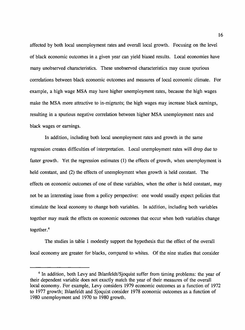
16

affected by both local unemployment rates and overall local growth. Focusing on the level

of black economic outcomes in a given year can yield biased results. Local economies have

many unobserved characteristics. These unobserved characteristics may cause spurious

correlations between black economic outcomes and measures of local economic climate. For

example, a high wage MS A may have higher unemployment rates, because the high wages

make the MSA more attractive to in-migrants; the high wages may increase black earnings,

resulting in a spurious negative correlation between higher MSA unemployment rates and

black wages or earnings.

In addition, including both local unemployment rates and growth in the same

regression creates difficulties of interpretation. Local unemployment rates will drop due to

faster growth. Yet the regression estimates (1) the effects of growth, when unemployment is

held constant, and (2) the effects of unemployment when growth is held constant. The

effects on economic outcomes of one of these variables, when the other is held constant, may

not be an interesting issue from a policy perspective: one would usually expect policies that

stimulate the local economy to change both variables. In addition, including both variables

together may mask the effects on economic outcomes that occur when both variables change

together. 4

The studies in table 1 modestly support the hypothesis that the effect of the overall

local economy are greater for blacks, compared to whites. Of the nine studies that consider

4 In addition, both Levy and Ihlanfeldt/Sjoquist suffer from timing problems: the year of their dependent variable does not exactly match the year of their measures of the overall local economy. For example, Levy considers 1979 economic outcomes as a function of 1972 to 1977 growth; Ihlanfeldt and Sjoquist consider 1978 economic outcomes as a function of 1980 unemployment and 1970 to 1980 growth.

17

this issue, six find stronger effects on blacks than on whites (Bound and Holzer; Freeman;

Bartik; Frey and Speare; Osterman; Mooney); two find similar effects on blacks and whites

(Ihlanfeldt; Welch); and one finds stronger effects on whites (Ihlanfeldt and Sjoquist).

The effects of local industrial mix on black economic outcomes are unclear from

previous studies. Six studies find evidence that local industrial mix makes a difference (the

two Eggers and Massey studies; Bound and Holzer; Cain and Finnic; Hughes; and Moore

and Laramore); two studies do not find significant effects of industrial mix (Ihlanfeldt;

Ihlanfeldt and Sjoquist). But 3 of the 6 studies that find industrial mix effects define their

industrial mix variables so that a change in the industrial mix variable will change overall

MSA employment. These three studies do not hold MSA employment growth constant (the

Eggers and Massey studies; Hughes). These three studies' industrial mix effects may

actually be due to the effects of faster MSA employment growth. For example, Eggers and

Massey (1992) use as an industrial mix variable the 1970-80 change in the ratio of operative

and crafts workers to the black population. Increases in operative and crafts workers in the

MSA will be associated with greater MSA employment growth, which is not held constant in

Eggers and Massey's regressions.

Of the remaining three studies that find industrial mix effects, two (Bound and

Holzer; Moore and Laramore) find some negative effects on blacks of a declining

manufacturing share. The Cain and Finnic study finds that black youths are helped by

increases in an MSA's youth oriented jobs.

18

The Spatial Mismatch Literature: Effects of Job Access on Black Economic Outcomes

The research literature on the effects on black outcomes of being spatially close to

jobs the "spatial mismatch" literature has recently been reviewed by Holzer (1991) and

Ihlanfeldt (1992). This type of research is hard to conduct, for two reasons. First, job

access is hard to measure. Second, the direction of causation between job access and black

economic outcomes is unclear. For example, persons who obtain good jobs may move to the

suburbs, where there is strong manufacturing growth. Access to manufacturing jobs may

appear to cause black economic success when the truth is that black economic success causes

improved job access.

Probably the best studies of the spatial mismatch hypothesis have been done by

Ihlanfeldt and Sjoquist (1989, 1990, 1991) and Ihlanfeldt (1992). Their studies focus on the

economic outcomes of black youths living at home, for whom it is most plausible that

residential location is "exogenous", that is that residential location is a cause rather than a

result of labor market experiences. 5 In addition, their studies measure job access in a

"neighborhood" using commuting travel times for a large sample of neighborhood residents.

Their studies also measure travel time for jobs for which black youth are likely to be

qualified. This measure of job access seems superior to alternative measures (jobs within 30

minutes commute, etc.). The Ihlanfeldt and Sjoquist studies find large effects on black

youths of spatial accessibility of jobs.

5Black youths living at home might be different from other black youths. This raises the possibility of selection bias. But it is unclear why selection bias would lead to biased estimates of the effects of job access. There is no obvious reason for the unobserved attributes of black youths living at home to differ between high-access and low-access neighborhoods.

19

But it seems premature to declare a consensus on the basis of the findings of one

group of researchers. Furthermore, the research by Ellwood (1986) finds the effect of job

access on youth employment rates to be small. Ell wood's research also uses travel time as

an access measure, and also focuses on youth economic outcomes. Ellwood's research

considers only Chicago while Ihlanfeldt and Sjoquist consider more cities, and Ellwood's

data and travel time measures may be more subject to measurement error than Ihlanfeldt and

Sjoquist's (Ihlanfeldt, 1992; Kasarda, 1989; Leonard, 1986). Still, Ellwood's findings do

raise some doubt about whether spatial access to jobs affects black economic outcomes.

III. Methodology and Data

The new research for this report examines how the changes over time in different

economic outcomes for different groups of blacks and whites in a metropolitan area are

affected by changes in several characteristics of metropolitan economic development. This

section outlines the methodology used and describes the construction of the variables used.

The technical appendix has more details on the methodology and data.

The methodology and data used here have some advantages over those of previous

research. First, the methodology is designed so that estimates will not be biased by

unobserved area characteristics that affect the level of economic outcome variables.

Unobserved area characteristics can cause spurious correlations between the levels of

economic outcome and economic development variables. Second, compared to previous

research, the analysis considers more groups and more types of economic outcomes.

20

Finally, the methodology defines the industrial mix class of economic development variables

so that industrial mix and metropolitan growth can change independently. The industrial mix

variables all depend on the types of industries in the metropolitan area, not the metropolitan

area's size or growth.

Specification of the Estimating Equations

The basic model is a regression model using pooled time series of cross sections.

The cases are MSA-year combinations, where "year" refers to one-year periods for which the

variables measure percentage change. Many versions of the model are used, one for each

dependent variable. In general, the time-series includes 16 periods, ranging from 1973-74 to

1988-89. The number of MS As included for a given period ranges from 34 in the early

1970s to over 200 in the late 1980s. The model includes a time dummy for each period

except the first. Other variables, both dependent and independent, generally measure one-

year percentage change in either an MS A mean economic outcome (e.g., average real

personal earnings) or some aspect of the MSA's economic climate that might be a causal

influence (e.g., manufacturing employment as a percentage of total MS A employment). The

dependent variables always describe a specific demographic group (e.g., black high school

dropouts). The estimation procedure corrects for both heteroskedasticity and serial

correlation. To correct for heteroskedasticity, cases are weighted using weights that are

based on the statistical precision with which the percentage change in MSA mean economic

outcomes are measured. This report's technical appendix gives more information on the

rationale behind pooling and on the validity of the heteroskedasticity corrections.

21

The basic equation is as follows:

%LYmu - a+b TIME t c(L)%^DEVEWPmt * ^

where %A7 is the dependent variable, expressed as a one-year percentage change in some

demographic group's MSA average economic outcome for the period that the particular

MSA-year case represents; TIME is a vector of one-year period dummies, one for each

period except the first; %ADEVELOP is a vector of independent variables, intended to

measure changes in various characteristics of the MSAs that describe its economic

development, broadly defined; m designates a particular MSA; t designates the time period; g

designates the demographic group being considered; a is the regression constant; b and c

represent the coefficients on the variables; c(L) is notation that indicates that some

specifications include lagged as well as current values of the economic development

variables, with the coefficients on these lagged variables estimated without constraints; and e

is the error term.

Controlling time dummies avoids making inferences based on national trends in the

economic outcome and economic development variables. These national trends could be

spuriously correlated. Instead, this study focuses on explaining differences from one MSA to

another in the year to year changes in economic outcomes. These MSA differences in the

change in economic outcomes are assumed to be in part caused by differences from one MSA

to another in the change in the economic development variables.

This specification has the advantage of eliminating possible biases due to fixed

unobserved MSA characteristics. For example, some MSAs may be low-wage areas because

they are attractive places to live; some might attract more high technology industries, because

22

they are attractive places to live. As a result, a high tech MSA industrial structure could be

negatively correlated with MSA wages, even though high tech employment does not cause

lower wages. But by focusing on year-to-year changes in measuring the dependent and

independent variables, the methodology eliminates any unobserved fixed MSA

characteristics. 6

The long-run effect on an economic outcome variable of a permanent change in an

MSA economic development variable is the sum of the coefficients on all current and lagged

values of that economic development variable. For example, suppose a specification includes

the current change in an economic development variable, the once-lagged change in that

same economic development variable, and the twice-lagged change. Then the cumulative

effect on the level of the economic outcome variable of a permanent 1 percent increase in the

economic development variable will at first be given by the coefficient on the current change,

after 1 year by the coefficient on the current change plus the coefficient on the lagged

change, and after 2 or more years by the sum of all three coefficients.

An important issue in specifying this model is how many lags of the economic

development variables to include. As more and more lags are added, estimates become more

and more imprecise. To choose an optimal lag length, this report will use Schwartz's

Bayesian Criterion (SBC), a standard model selection criterion. Geweke and Meese (1981)

present arguments for the superiority of the SBC over other model selection criteria.

6 There could of course also be unobserved MSA characteristics that change in some systematic way over the time period being analyzed. These MSA fixed trend effects could cause bias in a changes specification. The technical appendix analyzes this issue further.

23

The SBC in the current report usually chooses models with only current changes in

economic development variables, and no lagged changes, particularly for black groups. The

choice of zero lags does not mean that the effects of economic development variables are

unchanged over time; it means that any changed effects are modest enough that including

them is not statistically optimal. To allow comparison across different groups and outcomes,

the emphasis in the report will be on the long-run estimated effects for the zero-lag

specification. Results for longer-lag specifications will be mentioned when the longer-lag

specification might lead to different inferences.

Dependent Variables

The data on the dependent variables, the percentage change in an MSA's average

economic outcomes, are derived from the Annual Demographic File of the Current

Population Survey from March 1974 to March 1990. Each Annual Demographic File

contains data on the "economic outcomes" (personal earnings, income, work, and so on) of

sampled persons and families during the preceding year. My procedure for constructing the

dependent variables began by calculating, for each economic outcome variable and

demographic group considered, a "regression-adjusted" mean for each identified metropolitan

area and each year that controlled the individual's characteristics. Each dependent variable is

then simply the percentage change from one year to the next of that "regression-adjusted"

MSA mean. 7

7 As noted in Table 2, the actual percentage change numbers used in the regression are calculated using as a base the overall mean of that adjusted economic outcome variable for that demographic group. This base was used because for some MSA-year cases the adjusted

24

Table 2 describes the dependent variables. Real annual personal earnings is the best

measure of a person's economic success. The other variables either measure things that

determine personal earnings (weeks worked, weekly earnings, etc.) or measure the person's

poverty status, which is strongly influenced by personal earnings. The groups considered

permit analysis of how the effects of economic development policies vary by race, education,

age, and gender.

The regression adjustment procedure worked as follows. For each year of the Annual

Demographic files, a number of regressions were estimated. The observations for each

regression were on individuals. The sample for each regression was all persons in identified

MS As in a particular demographic group, such as black males 16 and over (see table 2).

Each regression had as a dependent variable some economic outcome measure, such as real

personal earnings. Each regression used as independent variables a number of personal

characteristics (education, experience, and gender) and a full set of dummy variables

identifying the person's metropolitan area. Using these regression coefficients for a given

outcome measure, year, and demographic group, I then predicted, for each metropolitan area

identified in the CPS in that year, what we would expect that economic outcome variable to

be for a person with "mean values" of personal characteristics. The means used for these

predictions were usually the mean values for blacks for these personal characteristics in

mean for some economic outcome variables and some demographic groups is less than or equal to zero. Calculating percentage change on a base of last year's value is not a sensible procedure for those cases. The technical appendix further discusses this issue of calculating percentage change. For the poverty rate variable, the "percentage" change in the year-to-year change in the adjusted percentage in poverty in the MSA, not the percentage change in that rate. For example, if black poverty changed from 30% to 27% in an MSA, this would be a decline of 3% and not 10%.

Table 2

Outline of Dependent Variables

TYPES OF DEPENDENT VARIABLES USEDOne-year percentage change in MSA's "adjusted mean" of annual real personal

earnings

Determinants of personal earnings:One-year percentage change in MSA's "adjusted mean" of annual weeks worked One-year percentage change in MSA's "adjusted mean" of annual weeks in labor

force One-year percentage change in MSA's "adjusted mean" of annual weeks

worked/weeks in labor force One-year percentage change in MSA's "adjusted mean" of average real earnings per

week One-year percentage change in MSA's "adjusted mean" of usual hours worked per

week One-year percentage change in MSA's "adjusted mean" of average real earnings per

hour worked

PovertyOne-year change in MSA's "adjusted mean" of poverty rate

GROUPS FOR WHICH DEPENDENT VARIABLES ARE CALCULATEDBlacks 16 and over Whites 16 and over

Black high school dropouts 25 and over Black high school completers 25 and over White high school dropouts 25 and over White high school completers 25 and over

Black youth: 16-24Black prime-age: 25-54Black older persons: 55 and overWhite youth: 16-24White prime-age: 25-54White older persons: 55 and over

Black males 16 and over Black females 16 and over White males 16 and over White females 16 and over

Notes: All real earnings/income figures are adjusted for estimated local prices, as described in technical appendix. Percentage change is calculated by dividing the one-year absolute change in a particular outcome measure by the sample mean of that outcome for that demographic group and then multiplying by 100. MSA means are "adjusted" using regression procedures described in text. High school completion/dropout status based on whether completed 12 years of school. Drop-out and completer groups only include persons 25 and older because younger persons are more likely to still be completing education.

26

1986. 8 For example, real personal earnings for whites in New York in 1977 are predicted

using the regression coefficients from the 1977 regression for real personal earnings. These

predictions estimate what earnings would have been for whites in New York in 1977 if their

education, experience, and proportion of each gender were the same as was true of the

average black in the U.S. in 1986.

For some groups and characteristics, it makes no sense to hold characteristics constant

at the overall black means in 1986. For example, it makes no sense to calculate what a

typical white 16 to 24-year old's earnings would have been if his experience had been at the

average black's experience level in 1986, or what the average white high school completer's

earnings would have been if he had been at the same education level as the 1986 black

average. Education by definition varies with status as a high school dropout and completer,

and experience by definition varies with the age group. For these groups and characteristics,

predictions used the black means for the comparable group in 1986. Thus, the white dropout

predictions for 1974 would use the mean education levels of black high school dropouts in

1986, and the white high school completer predictions would use the mean education of black

high school completers in 1986; all other individual characteristics would still be kept

constant at the overall 1986 black mean.

The dependent variable for each equation is the year to year percentage change in an

MSA in the predicted value of one of the economic outcome variables. An alternative would

have been to simply use the year to year percentage change in the MSA's mean value of that

8 1986 was somewhat arbitrarily chosen as a reference point, simply because the empirical work began using the March 1987 CPS.

27

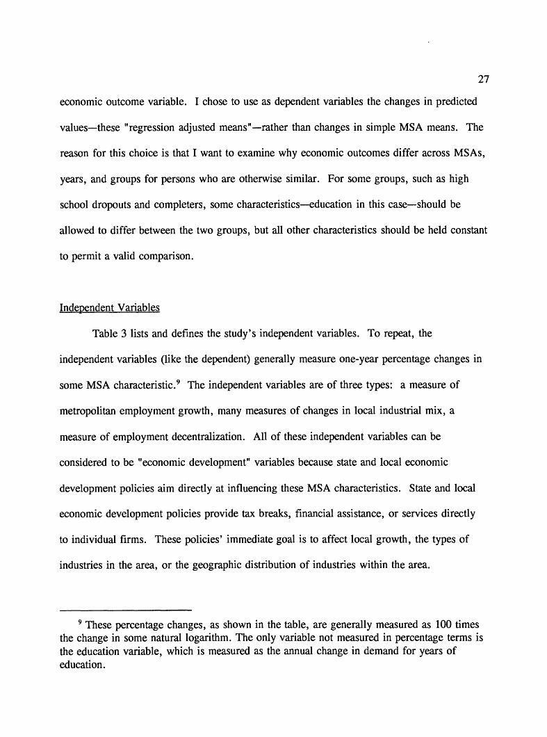
economic outcome variable. I chose to use as dependent variables the changes in predicted

values these "regression adjusted means" rather than changes in simple MSA means. The

reason for this choice is that I want to examine why economic outcomes differ across MSAs,

years, and groups for persons who are otherwise similar. For some groups, such as high

school dropouts and completers, some characteristics education in this case should be

allowed to differ between the two groups, but all other characteristics should be held constant

to permit a valid comparison.

Independent Variables

Table 3 lists and defines the study's independent variables. To repeat, the

independent variables (like the dependent) generally measure one-year percentage changes in

some MSA characteristic. 9 The independent variables are of three types: a measure of

metropolitan employment growth, many measures of changes in local industrial mix, a

measure of employment decentralization. All of these independent variables can be

considered to be "economic development" variables because state and local economic

development policies aim directly at influencing these MSA characteristics. State and local

economic development policies provide tax breaks, financial assistance, or services directly

to individual firms. These policies' immediate goal is to affect local growth, the types of

industries in the area, or the geographic distribution of industries within the area.

9 These percentage changes, as shown in the table, are generally measured as 100 times the change in some natural logarithm. The only variable not measured in percentage terms is the education variable, which is measured as the annual change in demand for years of education.

Table 3

Description and Definition of Economic Development Variables

MSA EMPLOYMENT GROWTH:

[ln(MSA employment in year /) - ln(MSA employment in year / - 7)] times 100. Employment data uses 1989 MSA definitions and comes from BEA's Regional Economic Information System.

MSA DECENTRALIZATION:

"MSA EMPLOYMENT GROWTH" - {[In(employment in county containing central city in year f) - ln(employment in county containing central city in year t- 7)] times 100}.

MSA WAGE PREMIUM CHANGE:

* imt ^r1 ' imt-1

where wt is estimated industry / percentage "wage premium" (difference between average wage in industry and what we would expect based on workers' characteristics) from Table IIof Krueger and Summers (1988), and s±mtis estimated share of two-digit industry / in total private non-agricultural employment in MSA m in year t. Krueger and Summers' wage premiums are differences in the logarithm of wages across industries, and are multiplied by 100 before being used in this study.

MSA EDUCATIONAL REQUIREMENTS CHANGE:

Ei' Simt ~ £ Ei' Simt-\i i

where Et is average years of education in 2-digit industry / calculated from March 1990 CPS, and Stnt is industry /'s share of total MSA employment.

Table 3 (Continued)

PERCENTAGE CHANGE IN SHARE OF MSA DEMAND FOR DEMOGRAPHIC GROUP j:

times 100 where Djmt = £ G.S,imt'

and Gy = proportion of 2-digit industry /'s employment that consists of persons in demographic group j. These proportions are calculated using data from March 1990 CPS on all persons 16 and over. Demographic group variables are defined for all groups listed in Table 2. For drop-outs and completers, G{j calculated based on all individuals 16 and over.

MSA Change in Manufacturing Share

This is simply defined as change from t -1 to t in the percentage of the MSA's total employment in manufacturing industries.

Note: All 2-digit industry numbers come from estimates based on ES-202 industry data and REIS data. Procedure for estimating suppressed industries is described in the technical appendix.

30

The overall growth and decentralization measures are straightforward. The growth

measure is the year to year percentage change in employment in the MSA. This study's

calculations of MSA growth use 1990 boundaries of MSAs. The decentralization measure is

the difference between the overall percentage growth in the MSA and the percentage

employment growth in the county containing the MSA's central city. This difference is also

equal to the percentage change in the ratio of MSA employment to employment in the MSA's

"central city" county. In MSAs in which employment is more rapidly moving to the

suburbs, this variable will take on larger values. If blacks have greater difficulty in getting

access, by transportation or information networks, to suburban jobs, then this

decentralization variable will be negatively correlated with black access to jobs. This

measure of access is crude compared to direct measures of job access, such as average

commuting time to jobs. But this decentralization variable is the best reflection of access

available on a year-to-year basis for many MSAs.

The local industrial mix variables are all measures of the MSA's "average" value of

industry characteristics, based on the MSA's industrial mix and national data on industries.

The "wage premium" changes variable measures how MSA wages would change due to due

to changes in the proportion of MSA employment in industries that pay well or poorly

relative to the worker's credentials. This calculation uses national data on wage premiums

by industry to calculate these changes in the average MSA wage premium. The educational

requirement change variable measures changes in the average years of education demanded in

the MSA, if each industry demanded workers with the same number of years of education as

they typically employ in the nation. The demographic change economic development

31

variables measure changes in the proportion of metropolitan employment demand for

different demographic groups. The calculation for this variable assumes that each industry in

the metropolitan area allocates the same proportion of its employment demand to that

demographic group as it did in the nation in 1989.

These industry mix variables are all meant to measure different ways in which

changes in local industry mix might affect local labor demand. National industry

characteristics are used in calculating these industry mix variable to avoid effects of local

labor supply conditions on these variables. For example, the percentage of industry

employment that goes to a particular demographic group in an MSA would be expected to

increase if the local labor supply of that group in the MSA increases.

Table 4 lists how some of these industry characteristics vary across industries. Most

industry characteristics vary as one might expect. Some manufacturing industries are high

wage premium, but so are certain service industries such as communications and public

utilities. Female employment is concentrated in particular service industries and in a few

manufacturing industries such as apparel. Educational levels are high in legal services,

banking, and civilian government agencies but low in eating and drinking places. Other

industry characteristics may be less familiar. The large concentration of black high school

completers in government, and in certain quasi-public utilities such as communications is of

interest, as is the concentration of black high school dropouts in eating and drinking places

and apparel and textiles.

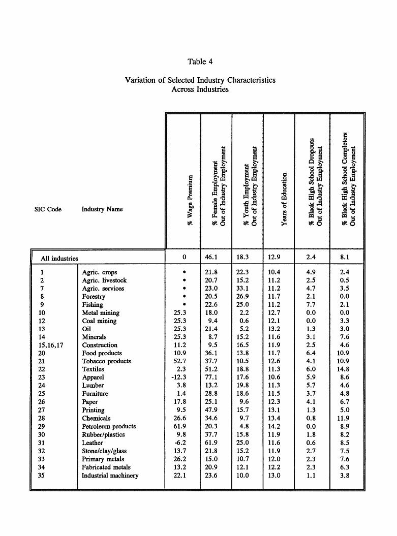
Table 4

Variation of Selected Industry Characteristics Across Industries

SIC Code Industry Name

All industries

1 2789

1012131415,16,1720212223242526272829303132333435

Agric. crops Agric. livestockAgric. servicesForestryFishingMetal miningCoal miningOilMineralsConstructionFood productsTobacco productsTextilesApparelLumberFurniturePaperPrintingChemicalsPetroleum productsRubber/plasticsLeatherStone/clay/glassPrimary metalsFabricated metalsIndustrial machinery

a1£1*

0

••••

25.325.325.325.311.210.952.72.3

-12.33.81.4

17.89.5

26.661.99.8

-6.213.726.213.222.1

•4-1ie55 «—<If*

^a* ^^

Ifr*S •§8 oSI

46.1

21.8 20.723.020.522.618.09.4

21.48.79.5

36.137.751.277.113.228.825.147.934.620.337.761.921.815.020.923.6

>v•«-» oit>jr» J"*K

ftw *§f 5 ;r" *•» :

18.3

22.3 15.233.126.925.02.20.65.2

15.216.513.810.518.817.619.818.69.6

15.79.74.8

15.825.015.210.712.110.0

J•3wj

1a*8

*

12.9

10.4 11.211.211.711.212.712.113.211.611.911.712.611.310.611.311.512.313.113.414.211.911.611.912.012.213.0

I-o >»1 tJy* *"**

sf^5 oPQ *>

2.4

4.9 2.54.72.17.70.00.01.33.12.56.44.16.05.95.73.74.11.30.80.01.80.62.72.32.31.1

•s *•»Qt a« g

r-> £|tJ^E *****s»tHM ^^

f— H OOQ ^

8.1

2.4 0.53.50.02.10.03.33.07.64.6

10.910.914.88.64.64.86.75.0

11.98.98.28.57.57.66.33.8

Table 4(Continued)

SIC Code Industry Name

36 3738394041424445464748495051525354555657585960,616263,64,65,6670727375

Electrical machinery Transport equipmentInstrumentsMisc. manufacturingRailroadsLocal transitTruckingWater transportAir transportPipelinesTransport servicesCommunicationsElectric/gas/sanitary svcsWholesale durablesWholesale nondurablesRetail — building materialsRetail — general merchandiseRetail — food storesAuto dealers/serviceClothing storesFurniture storesEating/drinking estab.Misc. retailBankingStockbrokersInsurance/real estateHotelsPersonal servicesBusiness servicesAuto repair/services

|*s1&,*

—13.5 26.716.73.4

26.816.016.016.016.016.016.029.333.62.52.5

-18.6-18.6-18.6-18.6-18.6-18.6-21.9-18.6

9.29.27.5

-19.4-19.4-3.1-8.7

** ftC3 O

|l& ^^v

j^j*S •!0 <*M

<o O

*s> I! ON O

42.6 22.442.649.27.4

33.416.213.132.60.9

61.550.224.928.330.928.772.550.821.176.236.357.559.569.443.254.963.069.648.614.3

I« oc *—<

P•jx£

w *1*3 ttM

5*

10.8 7.7

10.816.70.4

10.613.115.411.30.0

12.69.65.9

14.314.225.436.541.220.337.623.049.426.215.411.712.519.720.516.420.6

11*oi?VI

13.0 12.913.011.812.312.512.112.713.713.913.913.413.313.112.912.412.411.812.312.713.011.712.913.715.213.612.012.213.811.8

|l(5 >»

Q

8 Q, B

t™

* -0"i c!jS O«*

0.8 1.70.81.00.03.93.01.10.70.00.00.31.21.22.71.02.13.21.42.41.65.01.10.40.40.74.43.51.83.0

CL £j

6 c £»— -S8 pfr j^'

2 &1£> <1^£*£$ O

£3

7.2 10.87.26.08.4

17.010.311.99.00.03.3

15.212.24.15.92.69.26.24.29.24.46.15.59.06.96.38.27.97.86.5

Table 4 (Continued)

SIC Code Industry Name

767879808182838486878889

100101102

Misc. repair Motion picturesAmusementHealthLegal servicesEducation servicesSocial servicesMuseumsAssociationsEngineering servicesPrivate household servicesServices, n.e.c.Federal civilianFederal militaryState/local government

6

14>

1

-8.7 -16.3-16.3-1.42.3

-21.6-33.0

2.32.3

-51.72.32.3

••

*j

ifS 0*

o w|£*•"} C3 CO ft*3

l> *o b M** s

16.0 48.643.679.655.863.681.460.152.548.685.548.642.87.8

56.7

1-*-» o1 "i1&«ItW iRJEJ jrt

||

13.8 16.439.513.112.019.118.722.010.516.427.216.48.8

27.710.5

d.2

i<**.o

1>•

12.0 13.812.513.715.414.913.113.214.113.810.513.813.813.514.2

1| -Oi 1"

V W

If_4^ .QI s*W -*->

1.4 1.82.42.90.41.83.17.22.51.8

14.61.81.70.02.1

& "S i

r- 1 *28 f*§ jsCO >>

Ofl tottS .P.j Cj

3|

5.07.85.5

10.74.98.4

11.54.85.27.88.07.8

16.417.211.4

Note: Wage premium numbers come from Krueger and Summers (1988), Table II. These "percentage wage differential" are actually 100 times the change in the log of the total compensation differential. Note that some of their categories include several 2-digit industries here. Other numbers are calculated from March 1990 CPS. To avoid problems of SIC definitional change, some SIC codes are combined: (36, 38); (60, 61); (63, 64, 65, 66); and (73, 78, 87, 89).

35

The Direction of Causation Issue

The policy issue motivating this report is the effect of changes in MSA economic

climate on persons' economic outcomes. The coefficients on the economic development

variables could be interpreting as reflecting this direction of cause and effect, from change in

MSA economic development to changes in economic outcomes. But causation could also go

in the reverse direction, from changes in persons' economic outcomes to changes in MSA

economic development. This reverse direction of causation biases the estimated coefficients.

For example, MSA employment growth would be expected to increase wages, contributing to

a positive correlation between growth and wage increases. But MSA wage increases may

discourage employment growth, contributing to a negative correlation between growth and

wage increases. In an equation with MSA wage change as a dependent variable, the

coefficients on MSA employment growth may reflect both directions of causation. The

coefficients may be biased estimates of the true effects of MSA employment growth on

wages.

This report does not attempt to untangle the direction of causation between MSA

economic development and economic outcomes. But previous research has suggested that

this theoretical econometric issue may not be of large practical importance. For example,

estimates in Bartik (1991) and Blanchard and Katz (1992) suggest that the biases caused by

ignoring the "endogeneity" of MSA economic development are modest.

36

IV. Preliminary Analysis of Trends in Dependent and Independent Variables

National Trends in "Regression-Adjusted" Personal Earnings for Large MSAs

To get a sense of the overall economic differences between blacks and whites, and to

get a sense of the effects of "regression adjustment," figures 1 and 2 show national average

trends for real personal earnings for blacks and whites. The national average personal

earnings numbers in figures 1 and 2 use only persons in the 33 metropolitan areas that are

consistently identified in the CPS from 1973 to 1989. Figure 1 shows simple weighted

national means over these 33 MSAs for each year; figure 2 shows weighted regression

adjusted means.

As shown in the regression adjusted figure 2, when education, age, and gender are

controlled, black earnings shows ups and downs but no strong consistent trend for the overall

1973-89 period. The overall black real earnings trend was slightly downward, with a decline

of 2.5% from 1973 to 1989. White earnings, with characteristics controlled, also showed no

strong trend for this period; there was just a slight increase of 0.1 percent from 1973 to

1989. Both black and white earners suffered large earnings losses during this period's two

recessions, in the mid-1970s and the early 1980s.

A comparison of figures 1 and 2 suggests that the regression adjustment procedure

has two main effects. First, the adjustment reduces the black-white differential, because

whites on average have better educations than blacks. But even after the adjustment—even

when we are comparing blacks and whites with similar characteristics—blacks still earn

considerably less than whites. Second, the adjustment eliminates almost all of 1973-89's

Figure 1: Trends in Black and White Real Personal Earnings, 1973-89

Real Personal Earnings $18,000

$16,000

$ 14,000

$12,000

$10,000

$8,000

$6,000

x'-

Whites

i i i73 74 75 76 77 78 79 80 81 82 83 84 85 86 87 88 89

YearsNote: Figures are weighted means for 33 MSAs, in 1989 dollars.

Figure 2: Trends in Black and White Real Predicted Personal Earnings, 1973-89, Holding Constant Individual Characteristics

Real Predicted Personal Earnings $18,000

$16,000

$ 14,000

$12,000

$10,000

$8,000

$6,000

Whites

i i i i i i j__i73 74 75 76 77 78 79 80 81 82 83 84 85 86 87 88 89

YearsNote: Figures are weighted, regression adjusted means for 33 MSAs, in 1989 dollars.

39

observed real earnings growth. The average education and experience of both blacks and

whites grew during the 1970s and 1980s, increasing both black and white earnings. By

controlling education and experience, we compare blacks in 1989 with blacks in 1973 who

had similar characteristics, and the same holds true for whites. Once we control education

and experience, there is no significant growth in real earnings for blacks or whites from

1973-89.

Table 5 reports the percentage growth in adjusted real earnings for various black and

white subgroups. Among blacks, many subgroups did especially poorly: dropouts, young

persons, older persons, and males. Among whites, the subgroups that did relatively poorly

included dropouts, older persons, and males. When we compare blacks and whites, blacks

did more poorly than whites among all subgroups, and considerably more poorly than whites

(8 percent or more "earnings growth" gap) among all subgroups except prime-age persons

and high school completers. These estimated trends seem generally consistent with those

found in other recent research. The other research shows widening of the black-white

earnings gap among various subgroups of blacks and whites (e.g., Bound and Freeman's

(1992) analysis of earnings trends for black and white younger males).

Differences in Economic Trends Across MSAs

These national trends conceal large differences in economic outcome trends in

different MSAs. The pattern of variation across MSAs differs between blacks and whites.

Figure 3 shows the percentage growth in adjusted personal earnings for blacks and whites for

Table 5

Estimated Percentage Change in Regression-AdjustedReal Personal Earnings, 1973-89,

Weighted Average Over 33 MSAs Consistently in CPS

Blacks Whites

Overall -2.5% 0.1%

High School Dropouts -33.7% -21.4%High School Completers 3.6% 5.4%

Youth 16-24 -9.5% 2.7%Prime Age 25-54 -3.7% 2.3 %Older GE 55 -16.4% -3.6%

Males -22.7% -13.9%Females 26.4% 41.6%

Notes: Although percentage change numbers for sub-groups may seem inconsistent with overall numbers, note that overall percentage change should at best only approximately be weighted sum—using initial earnings shares of sub-groups as weights—of subgroup percentage changes. So, for example, overall white percentage change puts greater weight on white males than on white females because white male earnings average much more than white female earnings. This is also true for blacks, but to a lesser extent. This approximate summation will also be inexact because: adjusted numbers for each sub-group and overall numbers are based on separate regressions, and adjustment procedure calculates adjusted means at different mean values of some individual characteristics; the education sub-groups only include individuals 25 and over, while all other groups and overall numbers are based on all individuals 16 and over.

Figure 3: Percentage Growth in Real Regression Adjusted Personal Earnings for Blacks and Whites, 10 Large MSAs, Late 1970s to Late 1980s

Baltimore

Chicago

Detroit

Houston

Los Angeles

Miami

New York

Newark

Philadelphia

Washington

-40 -30 -20 -10 0Percentage Growth

10 20 30

Note: Percentage growth is calculated from 1976-79 average to 1986-89 average. Standard errors of percentage growth are in parentheses. Technical appendix describes construction of standard errors.

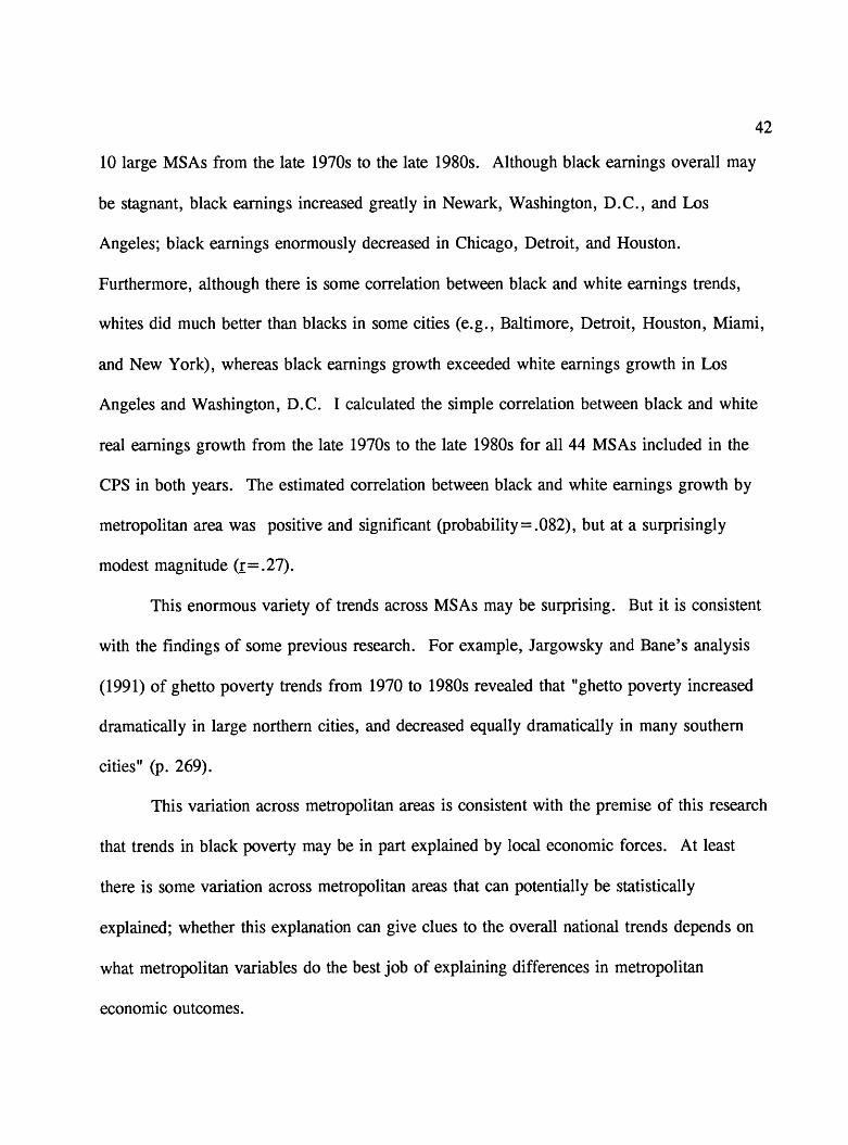
42

10 large MSAs from the late 1970s to the late 1980s. Although black earnings overall may

be stagnant, black earnings increased greatly in Newark, Washington, D.C., and Los

Angeles; black earnings enormously decreased in Chicago, Detroit, and Houston.

Furthermore, although there is some correlation between black and white earnings trends,

whites did much better than blacks in some cities (e.g., Baltimore, Detroit, Houston, Miami,

and New York), whereas black earnings growth exceeded white earnings growth in Los

Angeles and Washington, D.C. I calculated the simple correlation between black and white

real earnings growth from the late 1970s to the late 1980s for all 44 MSAs included in the

CPS in both years. The estimated correlation between black and white earnings growth by

metropolitan area was positive and significant (probability=.082), but at a surprisingly

modest magnitude (r=.27).

This enormous variety of trends across MSAs may be surprising. But it is consistent

with the findings of some previous research. For example, Jargowsky and Bane's analysis

(1991) of ghetto poverty trends from 1970 to 1980s revealed that "ghetto poverty increased

dramatically in large northern cities, and decreased equally dramatically in many southern

cities" (p. 269).

This variation across metropolitan areas is consistent with the premise of this research

that trends in black poverty may be in part explained by local economic forces. At least

there is some variation across metropolitan areas that can potentially be statistically

explained; whether this explanation can give clues to the overall national trends depends on

what metropolitan variables do the best job of explaining differences in metropolitan

economic outcomes.

43

National Trends in Economic Development Variables

The national trends in these metropolitan industry mix variables generally are what

one would expect. The female and youth employment demand variables show increases over

time due to the shift to services. Average educational requirements have gone up as the

economy has shifted to higher education industries. Figure 4 shows the trends in a less

familiar variable, the wage premium variable. This variable has declined considerably,

dropping about one-and-a-half percent from the late 1970s to the late 1980s.

The trends in the black employment demand variables are more surprising. The black

high school completer demand variable has declined over time, while the black high school

dropout demand variable has increased (Figures 5 and 6). Black high school completer

demand appears to have stagnated in large part because of sluggish employment growth in

government and the quasi-government communication industry. These industries employ

large shares of black high school completers.

Black high school dropout demand has held up due to increased demand for

employment in eating and drinking establishments and private household services. These are

industries in which black high school dropouts have particularly large shares. 10 In the

overall economy, employment is shifting towards industries that employ more high school

completers compared to high school dropouts. But the industry distribution of blacks by

educational level differs greatly from that of whites. Industry shifts are not increasing the

10 These statements about the causes of these trends are based on a decomposition of the causes of these trends by industry, which is presented in the technical appendix.

Figure 4: Trends in Average MS A Industry Wage Premiums,All MSAs

Average MSA Industry Wage Premium (Percent) 1.0

0.5

0.0

-0.5

-1.0

-1.575 76 77 78 79 80 81 82 83 84 85 86 87 88 89

YearsNote: All numbers are averages over 316 MSAs weighted by MSA total employment.

Figure 5: Trends in Average Industry MixPrediction of Proportion of Employment Demand

for Black High School Completers, All MSAs

Demand Share for Black High School Completers (Percent)

8.50

8.45

8.40

8.35

8.30

8.25

8.20 I I I I

75 76 77 78 79 80 81 82 83 84 85 86 87 88 89

Years

Note: All numbers arc averages over 316 MSAs weighted by MS A total employment.

Figure 6: Trends in Average Industry MixPrediction of Proportion of Employment Demand

for Black High School Dropouts, All MSAs

Demand Share for Black High School Dropouts (Percent)

2.260

2.255

2.250

2.245

2.240

2.235

2.23075 76 77 78 79 80 81 82 83 84 85 86 87 88 89

Years

Note: All numbers axe averages over 316 MSAs weighted by MSA total employment.

47

demand for black high school completers compared to black high school dropouts. This

surprising trend has previously been noted by Bound and Freeman (1992).

Variations in Economic Development Trends Across MSAs

The change across MSAs in these measures of economic development shows

considerable diversity across MSAs, and the different economic development measures show

some independence. Table 6 shows the 1979-89 change in selected economic development

variables for 11 large MSAs. These MSA include the 10 MSAs for which economic

outcome changes were previously presented in figure 3; Boston is included as a well-known

case in which metropolitan growth was quite healthy from 1979 to at least 1988. Although

the qualitative trends are often similar, the magnitude of these economic development trends

often differ considerably. For example, most MSAs tended to suffer from a reduced average

wage premium, but in MSAs such as Detroit the decline was worse. There is also some

independence of the measures; for example, Boston suffered from considerable

deindustrialization, yet its wage premium during the 1980s stayed almost the same.

The interrelationship among a number of these variables is further explored in table

7, which provides a correlation matrix across MSAs for the 1979-89 changes in many of

these variables. Growth tends to be strongly positively correlated with change in the wage

premium, and strongly negatively correlated with change in female labor demand. The wage

premium variable is strongly positively correlated with growth and increases in the

manufacturing share; it is negatively correlated with changes in female and youth demand.

The education and high school dropout variables are not strongly correlated with any other

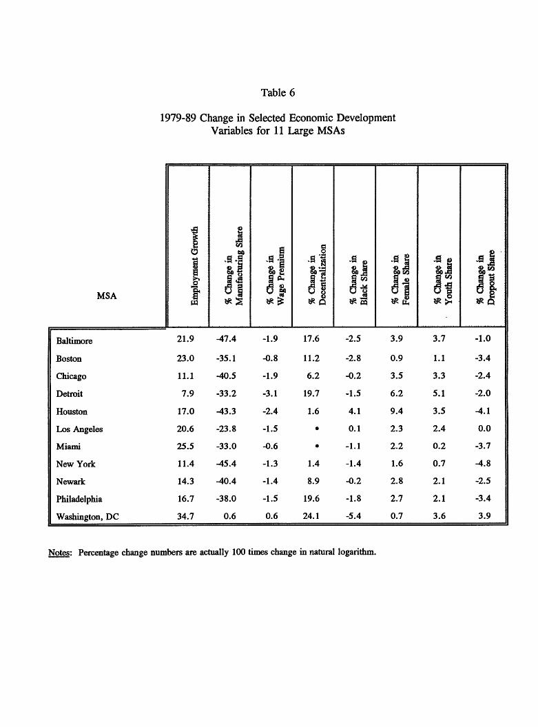
Table 6

1979-89 Change in Selected Economic Development Variables for 11 Large MS As

MSA

Baltimore

Boston

Chicago

Detroit

Houston

Los Angeles

Miami

New York

Newark

Philadelphia

Washington, DC

O

1ttW

21.9

23.0

11.1

7.9

17.0

20.6

25.5

11.4

14.3

16.7

34.7

en6Q

— ' o

T\ 2•^1 G^5

-47.4

-35.1

-40.5

-33.2

-43.3

-23.8

-33.0

-45.4

-40.4

-38.0

0.6

Sa ,260 £

|^^ I?

-1.9

-0.8

-1.9

-3.1

-2.4

-1.5

-0.6

-1.3

-1.4

-1.5

0.6

cJ

•4> 4Meo -a§ |

S

17.6

11.2

6.2

19.7

1.6

•

•

1.4

8.9

19.6

24.1

-S g**JiJD isjj

^

-2.5

-2.8

-0.2

-1.5

4.1

0.1-1.1

-1.4

-0.2

-1.8

-5.4

-S |

t 60

1i

3.9

0.9

3.5

6.2

9.4

2.3

2.2

1.6

2.8

2.7

0.7

J~

IN

3.7

1.1

3.3

5.1

3.5

2.4

0.2

0.7

2.1

2.1

3.6

J .

w

1 1C

-1.0

-3.4

-2.4

-2.0

-4.1

0.0-3.7

-4.8

-2.5

-3.4

3.9

Notes: Percentage change numbers are actually 100 times change in natural logarithm.

Table 7

Means, Standard Deviations, and Correlations of Changes in Selected Economic Development Variables, 1979-89

% Change in Employment% Change in Manufacturing Share% Change in Decentralization% Change in Wage Premium% Change in Female Share% Change in Black Share% Change in Dropout Share% Change in Youth ShareChange in Educational Requirements

Mean

19.3-24.2

2.8-1.7 4.8 0.0

-1.9 3.2

.065

Standard Deviation

15.316.96.51.33.42.73.12.9

0.051

# of Observations

314314140314314314314314314

% Change in Employment

% Change in Manufac. Share

% Change in Decentralization

% Change in Wage Premium

% Change in Female Share

% Change in Black Share

% Change in Dropout Share

% Change in Youth Share

60

•*i<O 3

llJl H

0-328 (0.0001)

0.056 (0.512)

-0.082 (0.336)

«f^

0.672 (0.0001)

0.562 (0.0001)

0.139 (0.100)

-0.572 (0.0001)

-0.211 (0.0002)

-0.104 (0.221)

-0.676 (0.0001)

-0.445 (0.0001)

-0.035 (0.540)

-0.104 (0.221)

-0.389 (0.0001)

0.581 (0.0001)

0.070 (0.214)

0.095 (0.092)

-0.026 (0.762)

-0.128 (0.023)

-0.006 (0.911)

-0.085 (0.132)

-0.474 (0.0001)

-0.421 (0.0001)

-0.048 (0.570)

-0.775 (0.0001)

0.373 (0.0001)

0.214 (0.0001)

0.236 (0.0001)

-0.287 (0.0001)

-0.226 (0.0001)

0.023 (0.792)

-0.153 (0.007)

0.338 (0.0001)

0.201 (0.0003)

-0.890 (0.0001)

-0.021 (0.717)

Table 7 (Continued)

Notes: All statistics are unweighted. " % changes" are really 100 times changes in natural logarithm of each variable. For correlation table, number in parentheses is probability of correlation that large in absolute value under null hypotheses that correlation is zero. Correlation based on 314 MS As, except for those involving decentralization, which are based on 140 MSAs.

51

variables, but are so strongly correlated with each other (negatively) that one variable clearly

can serve as a proxy for the other one. The change in black labor demand is most strongly

positively correlated with changes in female labor demand. 11

These correlations are high enough to reemphasize that these different economic

development variables should not be looked on as independent of one another. These

economic development variables are probably causally linked. For example, growing MS As

may tend to have predictable changes in industrial mix, and certain types of changes in

industrial mix may be favorable towards growth. 12 On the other hand, the correlations are

not large enough to prevent possible inferences about which economic development

characteristics have the most powerful effects on black and white economic outcomes.

I also used some regressions to describe the pattern of change in these economic

development variables across different regions and MS A sizes (table 8). These regressions

each used the 1979-89 percentage change in one of the economic development variables for

an MSA as the dependent variable. The independent variables were different polynomials in

the 1979 employment size of the MSA, and dummy variables for the MSA's regions. Larger

size is associated with greater employment growth for MS As near in size to the mean MSA,

although increased size decreases growth for the largest MS As. 13 Larger MS As also

11 These statements about "strong" correlations somewhat arbitrarily consider a "strong" correlation to be one that is greater than 0.5 in absolute value.

12 In Section VI, I present some evidence that growth and increases in the wage premium have a mutual cause-and-effect relationship, and discuss some reasons for such a relationship.

13 The MSA with the mean natural log of employment in 1979 has employment around 144,000. The derivative of 1979-89 growth with respect to 1979 size is positive up to about 6.4 times the size of the mean MSA, or up to around 922,000 in MSA employment. Only a few MS As have total employment exceeding 922,000.

Table 8

Estimates of How 1979-89 Changes in MSA EconomicDevelopment Variables Are Related

to 1979 MSA Size and Region of MSA

Independent Variables

Intercept

Percentage Deviation of (MSA Employment in 1979) from mean over all MSAs

Deviation2 times 10"2

Deviation3 times 10"4

New England

Mid Atlantic

East North Central

West North Central

East South Central

West South Central

Mountain

Pacific

South Atlantic

Significance of F-test for Employment Variables

Significance of F-test for Region Dummies

Dependent Variable

% Employment Growth00 W)

M

'a i « &GO CO 3 4>

-S % Change in Youth Share

Change in Educational

Requirements

18.9 -23.3 -1.7 5.0 0.01 3.0 0.064 (16.78) (-18.15) (17.16) (18.68) (0.06) (13.25) (15.01)

0.007

0.0001

0.038 (3.39)

0.012 (1.03)

-0.008 (-1.81)

3.4 (1.06)

-6.1 (-3.09)

-9.0 (-5.73)

-2.5 (-1.02)

-2.8 (-1.00)

-4.6 (-2.52)

5.0 (1.75)

8.5 (4.06)

12.1 (7.33)

-0.032 (-2.51)

-0.015 (-1.13)

0.006 (1.22)

-13.8 (-3.76)

-14.3 (-6.30)

-3.2 (-1.80)

4.2 (1.53)

6.1 (1.93)

1.4 (0.66)

8.6 (2.64)

10.6 (4.43)

2.2 (1.15)

0.001 (1.01)

0.0002 (0.17)

0.00002 (0.05)

0.2 (0.68)

-0.6 (-3.48)

-0.7 (-5.27)

0.03 (0.13)

0.08 (0.31)

0.05 (0.29)

0.3 (1.36)

0.6 (3.48)

0.6 (3.78)

-0.005 (-1.79)

-0.003 (-1.11)

0.001 (0.90)

-2.5 (-3.22)

-0.5 (-0.96)

0.5 (1.23)

0.2 (0.29)

-0.5 (-0.78)

2.7 (6.14)

1.2 (1.73)

-1.3 (-2.60)

-1.2 (-2-95)

-0.007 (-3.83)

-0.0005 (-0.28)

0.0007 (0.95)

-1.7 (-3.12)

-0.5 (-1.43)

0.6 (2.10)

1.1 (2.62)

-0.7 (-1.39)

2.2 (6.82)

0.9 (1.79)

-0.5 (-1.42)

-1.9 (-6.53)

-0.003 (-1.41)

0.002 (0.81)

-0.0006 (-0.69)

-0.5 (-0.72)

1.3 (3.27)

1.2 (3.67)

-0.2 (-0.44)

1.1 (2.01)

-0.7 (-1.98)

-1.8 (-3.11)

-1.5 (-3.45)

-0.2 (-0.52)

0.000004 (0.10)

0.000003 (0.06)

0.000004 (0.25)

0.016 (1.32)

0.003 (0.35)

-0.005 (-0.80)

-0.004 (-0.49)

-0.021 (-1.97)

0.024 (3.46)

0.002 (0.19)

-0.022 (-2.71)

0.002 (0.33)

0.022 0.313 0.068 0.0003 0.107 0.833

0.0001 0.0001 0.0001 0.0001 0.0001 0.0040

Table 8 (Continued)

Note: All estimates are based on 314 MSAs. Dependent variable is 100 times change from 1979 to 1989 in natural logarithm of each variable, except for education, which is in years, /-statistics are in parentheses. F-test probabilities are probabilities of F-test statistic for a group of variables under null hypothesis that all coefficients in that group are zero. Employment deviation variable defined as [100 times ln(1979 MS A employment)] minus mean of that variable over all MSAs. So, elasticity at mean with respect to 1979 employment is given by deviation coefficient. Region dummies are constrained so that their weighted sum, using number of MSAs in each region as weight, is zero. As discussed by Kennedy (1986), this implies that each region coefficient is the difference of that region from the national average.

54

have a greater tendency to lose manufacturing and decentralize, as well as a greater tendency

to lose industries that employ a great many blacks. The regional pattern is somewhat more

complicated. Generally, there was more growth in Sunbelt states, with the exception of

some of the "Oil Patch" states in the Southwest. Deindustrialization was particularly

pronounced in the Northeast, but New England MSAs were able to keep their wage premium

relatively stable. The Midwestern MSAs did not lose as much manufacturing share as the

national average but tended to lose high wage premium industries.

Finally, I examined how the economic development variables changed in MSAs with

relatively large black populations, compared to other MSAs. Table 9 reports the weighted

average changes for all MSAs, from 1973 to 1979 and from 1979 to 1989, in various

economic development variables, using as weights the black population shares in each MS A,

or the white population shares in MSAs. The most noticeable difference is that blacks tended

to be concentrated in MSAs that exhibited relatively slow employment growth. This black

concentration in slow-growth MSAs was especially pronounced in the 1973-79 period. This

pattern of black concentration in slow growth metropolitan areas was previously noted by

Frey and Speare (1988) and Moore and Laramore (1990).

V. Effects of MSA Growth on Black and White Economic Success

I now present estimates of the effects of changes in MSA economic development

variables on changes in black and white economic outcomes. As a reminder, the dependent

variables in this study are various types of year to year changes in MSA mean economic

outcomes—such as the year to year change in real personal earnings—for different

Table 9

Comparison of Average Change Across All MSAsin Selected Economic Development Variables,

Using Black or White Population Weights

1973-79 1979-89

% Employment Growth

Change in Percentage Wage Premium

Change in Educational Requirements

% Change in Black Share of Employment Demand

% Change in Female Share

% Change in Youth Share

Black Weights

12.7%

NA

NA

NA

NA

NA

White Weights

15.8%

NA

NA

NA

NA

NA

Black Weights

21.1%

-1.5%

+ .070 years

-1.0%

+3.7%

+2.5

White Weights

22.4%

-1.5%

+ .067 years

-0.7%

+3.9%

+2.7%

Notes: All numbers are based on 314 MSAs. Weights used are sum of black or white March 1990 CPS weights for each MSA.

56

demographic groups. These MSA mean economic outcomes are "regression-adjusted"

means: the means control education, experience, and other personal characteristics so that

we are comparing average economic outcomes over time and from one MSA to another for

persons with the same characteristics. The independent variables include time dummies, and

year to year changes in various MSA characteristics. These changes in MSA characteristics

include MSA employment growth, changes in MSA industrial mix, and changes in MSA

decentralization. All of these changes in MSA characteristics can be considered to be

changes in MSA economic development, broadly defined: an MSA economic development

policy that aids particular firms will have as its immediate goal affecting the growth of the

MSA, the types of industries in the MSA, or the spatial distribution of industries in the

MSA. In addition to including current values of these changes in MSA economic

development variables as independent variables, some specifications also include as

independent variables some lagged values of changes in economic development variables.

The present section, section V, begins with models in which the only economic

development variable among the independent variables is MSA employment growth. All

models include the time dummies. Section VI will present slightly more complex models

that also include as independent variables various types of MSA industrial mix variables, in

addition to MSA employment growth and the time dummies. Section VII will present even

more complex models that also include as an independent variable the decentralization

variable, in addition to MSA employment growth, an MSA industrial mix variable, and the

time dummies.

57

Several rationales can be offered for this estimation strategy of starting with simple

models before adding in more economic development variables. First, there are many

changes in MSA economic development variables that are potential independent variables.

Including all or even most of these variables in a model results in multicollinearity and

imprecise estimates. Being selective in what variables to include is essential to obtain

meaningful results. Second, as argued in section III, the MSA decentralization variable is a

crude measure of MSA job access or the within-MSA spatial distribution of industry. The

crudeness of this variable justifies initially excluding it from the estimated models. Third,

more time periods of data are available for the MSA employment growth variable than for

the MSA industrial mix variables. Data on employment growth are available back to 1969-

70. Data on changes in MSA industrial mix are available back to 1975-76. 14 Models that

only include MSA employment growth and time dummies as independent variables can be

estimated using a larger sample than models that also include MSA industrial mix variables.

Fourth, I would argue that local employment growth is the most important goal of most

economic development policy makers. A change in MSA industrial mix is only sometimes a

secondary goal. Policy makers might be interested in knowing the effects of MSA

employment growth, without control of changes in MSA industrial mix. Such estimates are

obtained in the present section.

14 The technical appendix gives more information on how these data are derived and the sources of these limitations.

58

Estimated Long-Run Effects of MSA Growth on Black and White Personal Earnings

Figure 7 reports estimated long-run effects of a 1 percent once-and-for-all increase in

MSA employment (compared to what it otherwise would have been) on black and white real

personal earnings. The model on which these estimates are based has as a dependent

variable the year to year change in average black (or white) real personal earnings in the

MSA. This MSA average controls education, experience, and other personal characteristics.

The figure 7 estimates are for a model in which the only independent variable, other than

time dummies, is the current year-to-year employment growth of the MSA. For blacks, this

"zero-lag" model is preferred applying Schwartz's Bayesian Criterion to 10 alternative

models that include various lag lengths in MSA employment growth. These 10 alternative

models also include, in addition to time dummies and current growth, from one to ten lags in

MSA employment growth. For example, the 2-lag model includes as independent variables

the time dummies, current employment growth, once-lagged employment growth, and twice-

lagged employment growth. For whites, the "once-lagged" model is preferred by the

Schwartz' Bayesian criterion. But figure 7 reports the zero-lag model for whites to make the

results comparable to those for blacks. The sensitivity of results to alternative lag lengths

will be considered further below.

As shown in figure 7, a 1 percent increase in MSA employment is estimated to

increase black real personal earnings by about 8/10ths of 1 percent and white real personal

earnings by about 5/10ths of 1 percent. The difference between these effects for blacks and

whites has a t-statistic value of 1.61. The probability of such a t-value occurring by chance,

when there is no true difference between effects on blacks and whites, is .107.

Figure 7: Long Run Effects of a 1 Percent Increase in MSA Employment on Black and White Regression Adjusted Real Personal Earnings

Zero-Lag Specification

Percent Effects on Adjusted Real Personal Earnings 1.0

0.5

0.0

.837% (.185)

.496% (.074)

Blacks Whites

Notes: Standard errors are in parentheses. Both coefficients are clearly statistically significant at all conventional significance levels. Reported percent effect is coefficient on the percentage change in MSA employment in equations with percentage change in real personal earnings of blacks or whites as dependent variables. Both equations include tune dummies. Estimates span 1973-74 to 1988-89, and include 1234 observations for blacks and 1432 observations for whites. As discussed in technical appendix, all estimates correct for heteroskedasticity and serial corrrelatioiL Zero-lag specification is optimal lag length for black model, based on Schwartz'sBayesian Criterion (SBC). One-lag specification is optimal for whites. For both blacks and whites, lag lengths from 0 to 10 years were tested. Long-run growth effect on white personal earnings is .477(.096) in one-lag specification.

60

Figure 8 shows alternative estimates of these "long-run" growth effects in a 10-lag

specification. Long-run effects do tend to decline somewhat in a 10-lag specification, to

perhaps half the estimated long-run effects in the zero-lag, specification. But growth effects

on both black and white real earnings are still statistically significant for at least nine years

after the employment change, and there is still some tendency for growth effects on black

real earnings to exceed those on white real earnings.

Figure 9 shows how MSA growth affects the various determinants of earnings. The

figure allows an evaluation of the relative contribution of these determinants to growth's

effect on earnings. Personal earnings is the product of annual weeks worked and average

earnings per week. Therefore, the percentage effect of growth on earnings will

approximately equal the sum of (a) the percentage effect of growth on annual weeks worked

and (b) the percentage effect of growth on average earnings per week. In turn, the

percentage effect of growth on annual weeks worked will approximately equal the sum of (a)

the percentage effect of growth on annual weeks in the labor force and (b) the percentage

effect of growth on the ratio of weeks employed to weeks in the labor force. Also, the

percentage effect of growth on earnings per week is approximately the sum of (a) the

percentage effect of growth on earnings per hour and (b) the percentage effect of growth on

hours per week. The purpose of this decomposition is to get some idea of whether growth

affects earnings by increasing work or increasing pay. Increasing work increases the size of

Figure 8Comparison of Alternative Estimates

of "Long-Run" Effects of a 1 % Increase in MSA Employment on Black and White

Regression-Adjusted Real Personal Earnings

1.6

1.4

1.2

1.370% -C.454X .

.837% (.185)

0.8

0.6

0.4

0.2

,4965. (.074)

Zero-lag 10-lag Cumulative effect Specification Specification after Last Significant

Lag in 10-lag Specification

I________________(9 years) |

Blacks

Zero-lag 10-lag Cumulative effect Specification Specification after Last Significant

Lag in 10-lag Specification

______ (10 years) I

Whites

Notes: Standard errors are in parentheses. All effects except 10-lag effectfor blacks are statistically significant at all conventional significancelevels. 10-lag specification, in addition to having more lags, has fewerobservations because observations can only start with 1979-80 asBEA's MSA employment data starts in 1969. Number of observations in 10-lagspecification is 1002 for blacks and 1200 for whites. All models alsoinclude time dummies.

% Effect on Weeks Employed/Weeks in Labor Force 294 % ***

(.084)

% Effect on Hours Per Week

.095%* (.063)

% Effect on .065% Earnings Per Hour (.297)

Figure 9A Decomposition of the Estimated Effects of

a 1 % Increase in MSA Employment on Personal Earnings Into Its Effects on Components of Earnings

Blacks% Effect on Weeks in Labor Force .372 % ***.

(.135)

% Effect on Annual Weeks Employed

% Effect on .837%*** Annual Earnings(.185)

% Effect on Weekly Earnings

.116% (.174)

Whites% Effect on Weeksin Labor Force .110%***.

(.046)

% Effect on Annual Weeks Employed

.248%*** (.049)

% Effect on Weeks Employed/Weeks in Labor Force 135 % ***"

(.018) % Effect on .496%*** Annual Earnings(.074)

% Effect on Hours Per Week

.067%*** (.028)

% Effect on Weekly Earnings

.255%*** (.065)

% Effect on .195%*** Earnings Per Hour (.067)

Notes: All estimates come from zero-lag specifications with different percentage change dependent variables, and same independent variables(time dummies and percentage change in MSA employment). Standard errors in parentheses. *, **, and *** indicate statistical

significance at 15%, 10% and 5% level for 2-tail test. Note that summations ofpercentage effects only approximately hold. Number of MSA-yearobservations is 1234 for blacks, 1432 for whites.

63

the market economy; increasing pay transfers resources from employers to employees. 15

Although earnings per hour is in the abstract the best measure of pay, this variable is quite

imprecisely measured in the CPS: the CPS only has a rough measure of average weekly

hours worked. Hence, earnings per week is a useful alternative measure of average pay.

The decomposition in figure 9 suggests that most of growth's effects on black

personal earnings are due to effects on work-related activities—labor force participation and

unemployment—rather than effects on pay levels. 16 There is some uncertainty about

estimated growth effects on black pay levels, but it is highly unlikely the effects on black pay

levels are as great as effects on black work activity. For whites, effects of growth on

personal earnings are about half due to effects on work activity and half due to effects on pay

rates. Growth helps blacks get into the labor market. Growth does that for whites too, but

apparently also helps whites move up to higher paying jobs.

Consequences for Poverty Rates of Growth's Effects on Personal Earnings

Figure 10 shows the effects of growth on black and white poverty rates. The effect

of growth on black poverty rates is over four times as great as the effect of growth on white

15 In turn, increasing pay may result in increasing prices, transferring resources from consumers to businesses. The point remains that wage increases by themselves simply lead to some redivision of the total economic pie. The exact redivision depends on what happens to consumer prices, but it still just a redivision of the same pie. Increases in labor force participation or employment rates can expand the size of the economic pie.

16 Note that this conclusion differs somewhat from Bartik (1991), which concluded that most of the black/white differences in growth effects on earnings were due to differential effects of growth on promotion to higher paying jobs. The reasons for the different conclusions in the two studies are unclear.

Figure 10: Estimated Long Run Reduction in Black and White Poverty Rate Due to 1 Percent Increase in MS A Employment, Zero-Lag Specification

Reduction in Poverty Rate (in Rate Points)

0.5

0.4

0.3

0.2

0.1

0.0

0.398

(.105)

0.072 (.024)

Blacks Whites

Notes: Standard errors are in parentheses. Both coefficients are clearly statistically significant at all conventional significance levels. " .398" coefficient is interpreted as implying (hat a 1 percent increase in MSA employment, in an MSA wiui 30 percent black poverty rate, would lower rate to about 29.6 percent. Estimates are based on 1234 MSA-time period observations for blacks, and 1432 MSA-time period observations for whites. Zero-lag specification is optimal according to SBC for both blacks and whites.

65

poverty rates. The black-white difference is highly significant statistically (probability =

.004). The greater effect of growth on black poverty rates compared to white poverty rates

in part reflects the greater effects of growth on black personal earnings vis-a-vis white

personal earnings. But the greater effect also reflects higher black poverty rates and

generally lower black personal earnings. With more blacks than whites close to the poverty

line, a given increase in personal earnings for blacks will tend to have greater effects on

poverty rates than a similar increase in earnings for whites.

Effects of Growth on the Earnings of Various Subgroups of Blacks and Whites

Figures 11, 12, and 13 present the estimated effects of growth on various subgroups

of blacks and whites, differentiated by education, age, and gender. In general, effects of

growth do not differ much among different groups of blacks. But growth effects for whites

are stronger for high school dropouts than for completers, and stronger for youths than for

prime-age and older persons. The black-white differential in growth effects is most

statistically significant for high school completers, prime-age persons, and females. In all

these cases growth effects for blacks are stronger than for whites.

One interpretation of these findings is that growth most strongly affects groups with

the weakest position in the labor market, such as high school dropouts, youths, and blacks.

These marginal groups are most dependent on a tight local economy to allow them to get

better jobs or indeed any jobs at all.

Figure 11Estimated Long-Run Percentage Effects

on Real Personal Earnings of 1 % Increase in MSA Employment, Blacks and Whites

Differentiated by Education

1.2

0.8

0.6

0.4

0.2

0

1.002% (.485)

.827% (.248)

.737%

.374% (.079)

Black HS Dropouts White HS Dropouts Black HS Completers White HS Completers

Notes: Standard errors are in parentheses. All effects are statistically significant at 5% level, 2-tail test, t -stats on selected comparisons have following probabilities of occurring by chance if true difference is zero: BDvs. BC: .744; WD vs. WC: .083; BD vs. WD: .859; BC vs. WC: .047. All models also include time dummies. Number of observations for different groups is as follows: BD, 1023; WD, 1432; BC, 1175; WC, 1432. Results reported are for zero-lag specifications. Zero-lag is optimal specification, according to SBC, among lag lengths from 0 to 10 years, for all groups except white completers, for whom optimal SBC lag length is one. One-lag estimates of LR growth effectsfor white completers is .348 (.100).

Figure 12

Estimated Long-Run Percentage Effectson Real Personal Earnings of 1 % Increasein MSA Employment, Blacks and Whites

Differentiated by Age

1.4

1.2

1.199% (.509)

0.8

0.6

0.4

0.2

16-24 25-54 GE55

Blacks H Whites

Notes: Standard errors are in parentheses. All effects except for B55 group are statistically significant at 5% level, 2-tail test. ?-stats on selected comparisons have the following probabilities of occurring by chance when thetrue difference is zero: B16 vs. B25: .668; B25 vs. B55: .864; W16 vs. W25: .157; W25 vs. W55: .796; B16 vs. W16: .800; B25 vs. W25: .075; B55 vs. W55: .827. All models also include time dummies. Number of observations for different groups is: B16, 1011; W16, 1432; B25, 1193; W25, 1432; B55, 982; W55, 1432. Reported estimates are for zero-lag specification. Zero-lag is optimal lag length according to SBC, among all lag lengths from 0 to 10 years, for all groups except whites 25-54 (W25), for whom one lag is optimal SBC lag length. For W25 group, LR growth effect in 1-lag specification is .357 (.119).

Figure 13: Estimated Long Run Effects of 1 Percent Increase in MSA Employment on Real Personal Earnings, Blacks and Whites Differentiated by Gender

Percent Effect on Real Personal Earnings1.0

0.9

0.8

0.7

0.6

0.5

0.4

0.3

0.2

0.1

0.0

.777 % (.243)

.513% (.087)

.833 % (.265)

.367% (.117)

Black Males

White Males

Black Females

White Females

Notes: Standard errors are in parentheses. All effects are statistically significant at 5% level, 2-tail test. 7-stats on selected comparisons have following probabilities: black males vs. black females: .864; white males vs. white females: .356; black males vs. white males: .419; black females vs. white females: .133. Estimates are based on following number of MSA-year observations: black males — 1166; white males — 1432; black females — 1192; white females — 1432. Zero-lag specification is optimal lag length, among lag lengths from 0 to 10 years, for all these groups except white males. For white males, a lag length of one is optimal. Estimated long-run effect of growth on white male earnings in one-lag specification is .464 (.112). All estimated models include time dummies.

69

Effects of Evening Out Growth

As pointed out above, the average black, compared to the average white, tends to live

in MS As with slower employment growth. Table 10 uses the estimated earnings effects of

growth to calculate how much more black personal earnings would have increased from 1973

to 1989 if blacks had lived in MSAs with the same average growth as whites. This

hypothetical change could have occurred either through increased job growth in MSAs with a

large black percentage (bringing jobs to people) or through migration of blacks to MSAs like

those of whites (bringing people to jobs).

Table 10 shows that evening out MSA growth among blacks and whites over the

1973-89 period would have increased the earnings of different black groups by 3 to 7

percent, or by 0.2 percent to 0.4 percent per year. This increase is large enough to be

important, but not large enough to explain all of the trends in black economic status. As

table 10 shows, the different MSA economic trends faced by blacks and whites can explain a

considerable portion, but not all, of the widening black-white earnings differentials in various

subgroups. 17

17 Also, it should be noted that these long-run effects of evening out growth might be cut in half if we relied on point estimates from a 10-lag specification rather than a zero-lag specification (e.g., Figure 8). However, 10-lag specification estimates are not precise enough to rule out the estimated effects presented in Table 10.

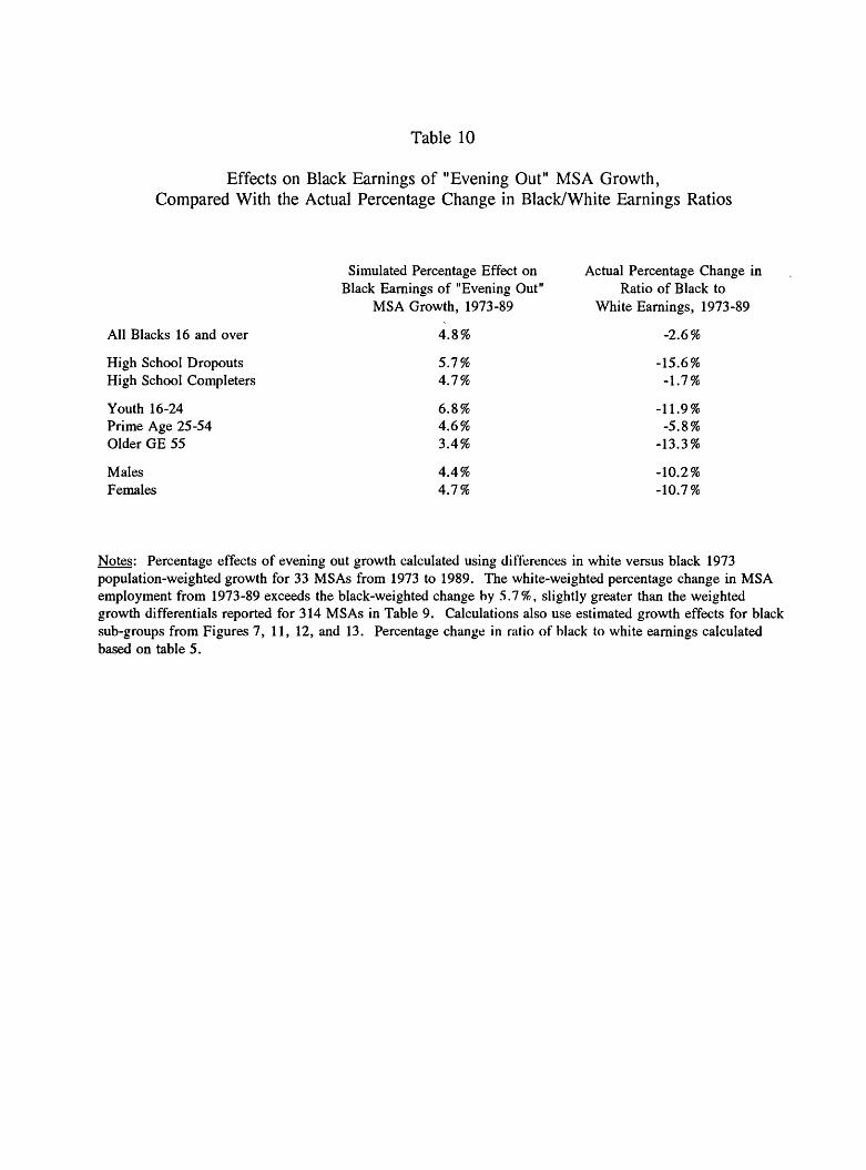
Table 10

Effects on Black Earnings of "Evening Out" MS A Growth, Compared With the Actual Percentage Change in Black/White Earnings Ratios

Simulated Percentage Effect on Actual Percentage Change inBlack Earnings of "Evening Out" Ratio of Black to

MSA Growth, 1973-89 White Earnings, 1973-89

All Blacks 16 and over 4.8% -2.6%

High School Dropouts 5.7% -15.6%High School Completers 4.7% -1.7%

Youth 16-24 6.8% -11.9%Prime Age 25-54 4.6 % -5.8 %Older GE 55 3.4% -13.3%

Males 4.4% -10.2%Females 4.7% -10.7%

Notes: Percentage effects of evening out growth calculated using differences in white versus black 1973 population-weighted growth for 33 MSAs from 1973 to 1989. The white-weighted percentage change in MSA employment from 1973-89 exceeds the black-weighted change by 5.7%, slightly greater than the weighted growth differentials reported for 314 MSAs in Table 9. Calculations also use estimated growth effects for black sub-groups from Figures 7, 11, 12, and 13. Percentage change in ratio of black to white earnings calculated based on table 5.

71

VI. Effects of Changes in MSA Industrial Mix on Black and White Economic Success

Strategy for Estimating the Effects of MSA Industrial Mix

As a reminder, the dependent variables in this study are the year to year change in the

average MSA economic outcome for various demographic groups. Most of the text

discussion and tables focus on one particularly important economic outcome variable, the

year-to-year change in average MSA real personal earnings per capita for a demographic

group. The models in this section continue to include as independent variables time dummies

and metropolitan employment growth. Also, the models in this section do not include a

metropolitan decentralization variable; models including a metropolitan decentralization

variable are considered in section VII. The models in this section do add in as independent

variables different variables that depend on changes in the MSA's industrial mix.

Simultaneously including as independent variables all the industrial mix variables

would lead to multicollinearity problems and imprecise estimates. My alternative strategy is

to add in the industrial mix variables as independent variables one at a time. Industrial mix

variables that are significant are kept in subsequent models that include additional industrial

mix variables; industrial mix variables that are statistically insignificant are dropped. All

models also include time dummies and MSA employment growth.

I begin this alternative modelling strategy by including as an independent variable the

change in the share of MSA jobs in manufacturing. Declining manufacturing is one of the

more popular explanations for black poverty problems. To anticipate the results below, this

variable has the expected effects at a statistically significant level only for some groups. I

72

then try an alternative industrial mix variable that I believe is theoretically superior to the

manufacturing share variable: the change in the average MSA wage premium due to

changing industrial mix. This wage premium variable attempts to capture how MSA wages

will change due to increases or decreases in industries that pay well relative to the credentials

of their workers. I would argue that this wage premium variable better measures the main

reason why the MSA's manufacturing share is argued to be important: MSA manufacturing

share reflects how many MSA jobs are "good jobs." Again anticipating results, this wage

premium variable appears to statistically dominate the manufacturing share variable.

I then add in separately, as independent variables, other industrial mix variables, to a

model that already includes as independent variables the time dummies, MSA employment

growth, and the wage premium variable. I first add in as an independent variable the change

in the share of MSA labor demand for a particular demographic group due to changes in

MSA industrial mix. I then drop this demographic share variable, and add in as an

independent variable the change in the years of education demanded by an MSA's employers

due to changes in the MSA's industrial mix. As the results will show, these demographic

share and education demand variables are generally not statistically significant.

At each stage of this estimation search strategy, I considered alternative lag lengths in

the economic development variables: the metropolitan employment growth variable and the

various industrial mix variables. I considered models with five different lag lengths, from

zero lags up to four lags. A zero lag model, for example, would include current year to

year MSA employment growth and the current year-to-year change in whatever industrial

mix variables were included in a particular specification. A two lag model would include

73

current MSA employment growth and current change in the MSA industrial mix variables,

once-lagged employment growth and once-lagged industrial mix variables, and twice-lagged

employment growth and twice-lagged industrial mix variables. Only a maximum of four lags

were considered, because the industrial mix variables are only measured starting with the

1975-76 time period. In general, zero lag models—models with only current values of

employment growth and industrial mix variables—were preferred to longer lag lengths by

Schwartz's Bayesian Criterion for most of the specifications considered. Exceptions will be

noted in the tables.

Effects of Alternative Measures of Industrial Mix on Real Personal Earnings

Table 11 presents the estimated effects of changes in the MSA manufacturing share on

the real earnings of various groups of blacks and whites. As a reminder, this model also

includes as independent variables the time dummies and MSA employment growth.

Decreases in the MSA manufacturing share do not have significant negative effects on blacks

overall or whites overall. Decreases in the MSA manufacturing share do have significant

negative effects on three important groups: white high school dropouts, black high school

completers, and black prime-age persons. 18 The estimates suggests that declining

manufacturing generally has more negative effects on a black group than on a comparable

white group.

18 "Significance" here means that the probability is less than .15 for a two-tail test, or a /-statistic greater than around 1.44 in absolute value.

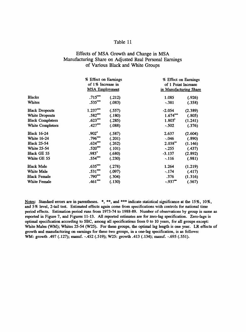
Table 11

Effects of MSA Growth and Change in MS AManufacturing Share on Adjusted Real Personal Earnings

of Various Black and White Groups

% Effect on Earnings % Effect on Earningsof 1 % Increase in of 1 Point IncreaseMSA Employment in Manufacturing Share

Blacks .715*" (.212) 1.085 (.926) Whites .535*** (.083) -.381 (.358)

Black Dropouts 1.237*" (.557) -2.054 (2.389)White Dropouts .582*** (.180) 1.674*** (.805)Black Completers .623*** (.285) 1.803* (1.241)White Completes .427*** (.088) -.502 (.376)

Black 16-24 .902* (.587) 2.637 (2.604)White 16-24 .796*" (.201) -.046 (.890)Black 25-54 .624*** (.262) 2.038** (1.146)White 25-54 .520*" (.101) -.255 (.437)Black GE 55 .983* (.680) -3.137 (2.892)White GE 55 .554*** (.230) -.116 (.981)

Black Male .635*** (.278) 1.264 (1.219)White Male .531*" (.097) -.174 (.417)Black Female .790*" (.304) .376 (1.316)White Female .461*" (.130) -.937** (.567)

Notes: Standard errors are in parentheses. *, **, and *** indicate statistical significance at the 15%, 10%, and 5% level, 2-tail test. Estimated effects again come from specifications with controls for national time period effects. Estimation period runs from 1973-74 to 1988-89. Number of observations by group is same as reported in Figure 7, and Figures 11-13. All reported estimates are for zero-lag specification. Zero-lags is optimal specification according to SBC, among all specifications from 0 to 10 years, for all groups except: White Males (WM); Whites 25-54 (W25). For these groups, the optimal lag length is one year. LR effects of growth and manufacturing on earnings for these two groups, in a one-lag specification, is as follows: WM: growth .497 (.127); manuf. -.452 (.519); W25: growth .413 (.134); manuf. -.695 (.551).

75

Table 12 presents the effects on real earnings of changes in an alternative measure of

MS A industrial mix, the average wage premium. The table 12 results are for a specification

that includes as independent variables the time dummies, MSA employment growth, and the

wage premium variable, but not the manufacturing share variable. The wage premium

variable has more statistically significant effects in table 12 than the manufacturing share

variable had in table 11. Declines in the average wage premium in an MSA lead to

significant declines in the real personal earnings of blacks overall, whites overall, white

dropouts, black high school completers, white youths, black prime-age persons, black males,

black females, and white females. 19 When both the wage premium and the manufacturing

variable are included in the estimation (table 13), the manufacturing variable is never

significantly positive for any group. In addition, the estimated effects of the wage premium

variable are usually not much affected by the inclusion of the manufacturing share variable.

Thus, the wage premium variable seems to dominate the manufacturing variable as a measure

of industrial mix.

Table 14 reports estimated effects on real earnings from a model that adds as an

independent variable the change in the share of MSA labor demand for the relevant

demographic group due to changes in the MSA's industrial mix. For each demographic

group, one demographic variable is added to the model. This demographic variable

measures demand change for the demographic group whose change in real earnings is being

used as the dependent variable. Each estimating equation also includes as independent

variables the time dummies, MSA employment growth, and the MSA wage premium

19 Again, "significance" here is a probability of less than .15 for a 2-tail test.

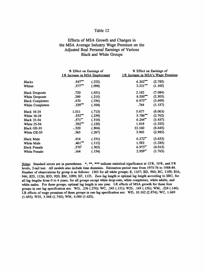
Table 12

Effects of MS A Growth and Changes inthe MSA Average Industry Wage Premium on the

Adjusted Real Personal Earnings of VariousBlack and White Groups

% Effect on Earnings of 1 % Increase in MSA Employment

Blacks Whites

Black Dropouts White Dropouts Black Completers White Completers

Black 16-24 White 16-24 Black 25-54 White 25-54 Black GE-55 White GE-55

Black Male White Male Black Female White Female

.547***

.377***

.720

.289

.470.329***

1.011.552***.571**.392***

-.320.365

.414.461***

.570*

.164

(.252)(.098)

(.651)(.215)(.336)(.104)

(.713)(.239)(.310)(.120)(.804)(.267)

(.331)(.115)(.365)(.154)

% Effect on Earnings of 1 % Increase in MSA's Wage Premium

6.202***2.221***

2.1828.550***6.973**.764

5.6775.786***6.244**1.819

12.1603.9026.272**1.5836.973**2.959**

(2.785)(1.105)

(7.084)(2.503)(3.699)(1.157)

(8.063)(2.762)(3.437)(1.355)(8.645)(2.985)

(3.653)(1.285)(4.013)(1.765)

Notes: Standard errors are in parentheses. *, **, *** indicate statistical significance at 15%, 10%, and 5% levels, 2-tail test. All models also include time dummies. Estimation period runs from 1975-76 to 1988-89. Number of observations by group is as follows: 1365 for all white groups; B, 1167; BD, 960; BC, 1109; B16, 946; B25, 1126; B55, 920; BM, 1099; BF, 1125. Zero lag length is optimal lag length according to SBC, for all lag lengths from 0 to 4 years, for all groups except white drop-outs, white completers, white adults, and white males. For these groups, optimal lag length is one year. LR effects of MSA growth for these four groups in one lag specification are: WD, .236 (.270); WC, .243 (.131); W25, .143 (.156); WM, .224 (.146). LR effects of wage premium of these groups in one lag specification are: WD, 10.162 (2.874); WC, 1.669 (1.455); W25, 3.568 (1.745); WM, 4.000 (1.625).

Table 13

Effects of MSA Growth, Changes in the MSA Manufacturing Share,and Changes in the MSA Wage Premium on the Adjusted Real

Personal Earnings of Various Black and White Groups

Blacks Whites

Black Dropouts White Dropouts Black Completers White Completers

Black 16-24 White 16-24 Black 25-54 White 25-54 Black GE-55 White GE-55

Black Male White Male Black Female White Female

Effect on Earnings of1% Increase in

MSA Employment

Effect on Earnings of 1 Point Increase in

Manufacturing Share

% Effect on Earnings of1 % Increase in MSA's

Wage Premium.541***.401***

.772

.281

.457

.355***

.951

.569***

.545**

.414***-.153.380

.403

.476***

.586*

.210

(.253)(.098)

(.654)(.216)(.338)(.104)

(.715)(.240)(.311)(.121)(.807)(.270)

(.332)(.115)(.366)(.154)

.292-1.004***

-2.736.401.612

-.974***

3.949-.7331.443

-1.023***-7.628***-.513

.656-.609-.840

-1.910***

(1.213)(.442)

(3.146)(.990)

(1.598)(.465)

(3.444)(1.097)(1.498)(.541)

(3.773)(1.215)

(1.591)(.518)

(1.747)(.698)

5.771***3.756***

6.8027.952***5.9712.247**

-1.1696.926***3.8453.382***

25.001***4.670

5.1772.509**8.385**5.879***

(3.455)(1.292)

(8.846)(2.906)(4.532)(1.354)

(10.035)(3.247)(4.246)(1.583)

(10.719)(3.496)

(4.522)(1.508)(4.974)(2.054)

Notes: Standard errors are in parentheses. *, **, and *** indicate significance at the 15%, 10%, and 5% levels for a 2-tail test. All models also include time dummies. All estimates are for a zero-lag specification. The estimation period is 1975-76 to 1988-89. The number of observations by group is identical to those given in the notes to Table 12.

Table 14

Effects of Shifts in the MSA Industry MixToward a Group on Adjusted Real Personal

Earnings of That Group

Blacks Whites

Overall -1.485 11.482***(1.380) (3.862)

Dropouts -2.488 0.162(2.321) (0.753)

Completers -0.458 2.732(1.458) (1.906)

Ages 16-24 0.809 2.497**(3.304) (1.419)

Ages 25-54 -0.166 6.769***(1.518) (2.649)

Ages GE 55 2.290 -0.656(2.143) (1.895)

Males 1.740 2.523***(1.289) (0.605)

Females -1.184 -2.149***(1.215) (0.755)

Notes: Reported effects are percentage effects on earnings of a percentage change in predicted share of a group—based on MSA industry mix—in total employment demand (e.g., shift from 10% share of employment for blacks to 11 percent is 10% increase). Standard errors are in parentheses. *, **, and *** indicate statistical significance at 15%, 10%, and 5% levels using a two-tail test. All estimates also control MSA growth, MSA wage premium, and time dummies. Estimation period runs from 1975-76 to 1988-89. Number of observations by group is identical to those given in Table 12. All estimates are for zero-lag specifications. Zero-lag specification is optimal specification according to SBC, among lag lengths from 0 to 4 years, for all groups.

79

variable. For the various black groups, there is no sign that shifts in the MSA industrial mix

towards industries that demand large proportions of that particular black group has significant

positive effects. The demographic share variables do have significantly positive effects for

some white groups. But the pattern of the coefficients suggests that these white demographic

variables are probably proxies for some unobserved variables that favorably affect industrial

mix. For example, the white demographic share and black demographic share variables are

almost perfectly negatively correlated. If one properly adjusts these variables for differences

in how they are defined, a shift towards a "white" demographic structure has approximately

the same magnitude positive effect on earnings for both blacks and whites. 20

Table 15 drops the demographic share variable, and adds in the education variable.

This education variable measures the change in education demand in the MSA due to changes

in the MSA's industrial mix. The models in table 15 continue to include as independent

variables the time dummies, MSA employment growth, and the MSA wage premium

variable. The education variable does not perform well. Increased education demand does

not appear to hurt the low-education dropout groups. Increased education demand is

estimated to adversely affect younger persons. But the regression adjustment procedure at

least in theory calculates the predicted real earnings of younger persons having the same

20 The black and white demographic share variables are the logged shares of these groups. Suppose that a shift in the unlogged white share (WS) has the same effect on the black and white earnings variables (BE and WE), or dBE/dWS=dWE/dWS=some constant k. Now by the definition of the unlogged black share variable (BS), dBS approximately equals -dWS. So dBE/dBS=-k. But the variables actually used in the regression are the logged shares. Under these assumptions, dBE/dln(BS)=-k*BS =-k(.107) at the mean of BS, and dWE/dln(WS)=k*WS=k(.860) at the mean of WS. Hence the ratio of the logged white demographic share variable's coefficient to the black coefficient should be .860/(-.107) = -8.04. The observed ratio in Table 14 is 11.482/(-l.485)=-7.73.

Table 15

Effects on Real Earnings of Shifts in An MSA's Industrial Mix Towards Higher Education Industries

Blacks Whites

Overall -0.347 -0.144(0.569) (0.225)

Dropouts 0.772 -0.192(1.468) (0.500)

Completers -0.026 -0.036(0.745) (0.236)

Ages 16-24 -3.453~* -1.072**(1.631) (0.573)

Ages 25-54 -0.367 -0.163(0.701) (0.275)

Ages GE 55 1.341 0.084(1.766) (0.606)

Males -0.525 -0.153(0.743) (0.262)

Females -0.155 -0.239(0.817) (0.359)

Notes: Reported effects show proportional effects on real earnings of 1 year increase in educational requirements, based on industry mix. For example, coefficient of -0.347 for all blacks means that 1-year increase in educational requirements—an enormous change—would reduce black earnings by 34.7%. Standard errors are in parentheses. *, **, and *** indicate statistical significance at 15%, 10%, and 5% levels for a two-tail test. All specifications also control MSA growth, the change in wage premium variable, and the time dummies. Estimation period runs from 1975-76 to 1988-89. Number of observations by group is given in Table 12. All reported estimates are for zero-lag specifications. Zero-lag is optimal specification according to SBC, among all lag lengths from 0 to 4 years, for all groups except white males. For white males, optimal lag length is one year. Long-run effect of education on white male earning in one lag specification is .207 (.326).

81

education as prime-age and older persons. It is unclear why increased education demand

should have more negative effects on younger persons than prime-age and older persons after

this adjustment.

Overall, these results are most consistent with the view that the most important MS A

industrial mix variable for black and white economic success is the average MSA wage

premium. Changes in MSA education demand, whether measured by changes in the share of

demand for high school dropouts or changes in average education levels of the typical MSA

industry, do not have the predicted adverse effects on low education groups.

The lack of effects of these education demand measures at the MSA level need not

imply that changing education demand has zero effects at the national level. The measures

of education demand mix used here are quite imperfect. Several researchers have argued

that educational requirements are increasing primarily because of changes within industries,

not because of changes in industry mix (Katz and Murphy, 1992; Bound and Johnson, 1992).

In addition, increases in education demand at the MSA level may be more easily

accommodated by in-migration of educated workers, the most mobile population group. For

both these reasons, the effects of national education demand increases could be greater than

the effects of this report's MSA education demand variables.

The earnings effects of the MSA wage premium could plausibly reflect the wage

premium's effects on both local wages and local labor supply. As shown in table 12, the

effect of reductions in the industry wage premium is more than 1-to-l: a 1 percent reduction

in the industry wage premium reduces white personal earnings by 2.2 percent and black

personal earnings by 6.2 percent. A 1 percent reduction in the MSA wage premium would

82

have exactly a 1 to 1 effect on earnings if each industry in the MSA paid the same as the

national average and persons' labor supplies were unaffected by a shift away from high wage

industries. But it is plausible that a shift away from high-wage industries in an MSA will

tend to reduce the average industry's wages in that MSA relative to its national counterpart.

Also, a shift away from high wage industries may tend to reduce labor force participation.

For both these reasons—reductions in relative MSA industry wages and reduced labor

supply—a percent reduction in the MSA wage premium might be expected to reduce average

MSA earnings by more than 1 percent. These hypotheses will be explored further below.

But of course these large industry wage premium effects may also occur because the wage

premium variable may be a proxy for other influences of MSA industry mix. As has been

shown by Dickens and Katz (1987), many industry characteristics—unionization for

example—are highly correlated with the industry wage premium. It is hard to distinguish

between hypotheses involving these highly correlated industry characteristics.

Further Exploration of the Effects of the MSA Industry Wage Premium on Personal Earnings

I now further explore how the average MSA industry wage premium affects black and

white earnings, and the consequences and implications of these effects of average MSA wage

premiums. To begin, figure 14 provides a decomposition of the effects of the industry wage

premium on overall black and white personal earnings into its effects on various determinants

of earnings. Wage premium effects for blacks are due more to wages going up than to work

activity going up. Wage premium effects for whites are due somewhat more to work activity

going up than to wages going up. One plausible interpretation of these black-white

Figure 14A Decomposition of How Changes

in the MSA Wage Premium Affect Real Earnings

% Effect on Annual Weeksin Labor Force 2.012

(2.035)

% Effect on Weeks Employed/Weeks in Labor Force _j 094

(L287)

% Effect on Hours Per Week

1.975*** (.904)

Blacks

% Effect onAnnual Weeks ,«Employed (2.252)

% Effect on Real Earnings

6.202*** (2.785)

% Effect on Earnings Per Week

6.498***

% Effect on 4.821 Earnings Per Hour (4.322)

% Effect on Annual Weeksin Labor Force .420

(.686)

% Effect on Weeks Employed/Weeks in Labor Force i 048***

(.269)

% Effect on .295 Hours Per Week (.387)

% Effect on .585 Earnings Per Hour (.926)

Whites

% Effect on „„«,***Annual Weeks }•»***Employed <•

% Effect on Real Earnings

2.221*** (1.105)

% Effect on .913/u J_>11«^VI. »J11 f ns:n\

Earnings Per Week ^52>

Notes: Standard errors are in parentheses. *, **, and *** indicate statistical significance at 15%, 10%, and 5% levels for a 2-tail test. Note that the various percentage effects only approximately add up. These results are based on specifications that control MSA growth and time dummies. Also, all results are for zero-lag specifications. The MSA growth decomposition from these specifications are quite similar to what was previously presented for specifications without the wage premium variable.

84

differences is that blacks have more difficulty than whites in getting access to high-wage

premium industries but that racial wage differentials are narrower within such industries.

Figure 15 reports the poverty consequences of changes in the average MS A wage

premium. The MS A wage premium does not have statistically significant effects on poverty

for blacks or whites, and for whites the estimated effect has an unexpected sign. One

plausible interpretation of these results is that persons on the margin of poverty do not have

access to high wage premium jobs, so the anti-poverty effect of shifts towards or away from

high wage industries is limited.

What are the policy implications of these estimated MSA industry wage premium

effects? It might appear that increasing the MSA wage premium is a more attractive option

than increasing MSA employment for state and local policymakers. As shown in table 13,

for many groups a 1 percent increase in the industry wage premium has a much greater

effect on real earnings than a 1 percent increase in MSA employment. For example, for

blacks overall, a 1 percent increase in the wage premium increases real earnings by over 6

percent, whereas a 1 percent increase in MSA employment increases real earnings by only

0.5 percent. But it is risky to just compare the coefficients on different variables. It is

probably far more costly for policymakers to increase an MSA's industry wage premium by

1 percent than to increase an MSA's wage premium by 1 percent. Increasing an MSA's

industry wage premium by 1 percent requires extremely large shifts in MSA industry mix.

For example, a 1 percent increase in an MSA's industry wage premium could be

accomplished by shifting 10 percent of the MSA's employment to industries that pay 10

percent more, which seems hard to do. In contrast, a 1 percent increase in MSA

Figure 15: Effectiveness of 1 % Increase in MSA Wage Premium in Reducing Black and White Poverty Rates

Reduction in Poverty Rate (in Rate Points)

2.0

1.5

1.0

0.5

0.0

-0.5

-1.0

1.685 (1.597)

1

-.306 (.363)

Blacks Whites

Notes: Standard errors are in parentheses. Estimated effects show reductionn poverty rate. For example, 1.685 effect for blacks means that a 1% increase in wage premium would reduce a black poverty rate mat was initially 20% to 18.315%. Estimates use 1234 MSA-year observations for blacks, and 1432 MSA-year observations for whites. All estimated models also include time dummies and MSA employment growth. Estimated models use a zero-lag specification.

86

employment may be achievable by feasible changes in state and local economic development

policies, according to the research literature reviewed in chapter 2 of Bartik (1991).21

Of course, it may not be possible to independently increase the MSA growth variable

and the MSA wage premium variable. These two variables could be causally related in

either direction. An increased MSA wage premium may increase the income of MSA

residents, resulting in increased consumer demand. This increased consumer demand may

lead to increased MSA employment in non-base industries such as retail industries. On the

other hand, MSA growth may tighten MSA labor markets, which may increase wages in the

average MSA industry compared to its national counterpart industry. These higher MSA

wages may discourage growth in the MSA by industries that are sensitive to wage costs.

These wage-sensitive industries tend to be industries in which pay is low relative to the

credentials required—low wage premium industries. The MSA's industry mix will shift

towards high wage premium industries.

Causality tests with this data base suggest that the causality runs both ways between

the MSA wage premium and MSA growth (table 16). These causality tests show particularly

21 There is another argument that it is more difficult to change the wage premium variable by 1 percent than to change the employment growth variable by 1 percent. The natural variation in the sample (the standard deviation in the sample) of the wage premium variable is far less than the natural variation of the employment growth variable (table 8). As a result, the beta coefficient—this report's coefficient times the ratio of the standard deviation of the independent variable to the standard deviation of the dependent variable—of the wage premium variable is usually about the same magnitude as the beta coefficient of the employment growth variable in most of the estimated models. It is plausible that the costs of changing some variable through policy are inversely related to the variable's standard deviation in the sample. If so, the smaller standard deviation in the sample of the wage premium variable than of the employment growth variable may indicate that it is more costly to change the wage premium variable than change the employment growth variable.

Table 16

Tests of Causation Between MSA Growth and Changes in the MSA Wage Premium

Direction of Causation Examined

Growth causing changes in Wage Premium

Changes in Wage Premium causing growth

Probability of F-test Statistic for Lagged "Causative" Variables___________

.0001

.0419

Notes: These regressions regress (1) growth and (2) changes in the wage premium on five lagged values of both variables. The relevant causality test is an F-test for whether the "other variable's" lagged values matter, once we control for lagged values of the dependent variable.

88

significant causal effects of MS A growth in increasing the MS A wage premium.

Thus, policy makers should realize that there may not be a clear tradeoff between

having more local growth and having higher "quality" local industries. Local growth and

higher quality local industries tend to go together. A successful growth strategy will make it

harder to pursue low-wage industries. Growth can be more easily sustained in the long run

by encouraging the growth of high-wage industries. A successful strategy of encouraging

high-wage industries will tend to encourage growth. A "growth" strategy and a "high-wage"

strategy should be viewed as complementary and not competing strategies.

The empirical results may also have implications for national policy towards high-

wage and low-wage-premium industries, although the case here is more unclear. The results

suggest, but do not prove, that national declines in high-wage-premium industries in the

1970s and 1980s may have hurt blacks more than whites. The results also suggest, but do

not prove, that a 1 percent national decline in average industry wage premium may, with

"spillover-multiplier" effects on other industries and labor supply, affect earnings by more

than 1 percent. The uncertainty arises because the estimates in this report, which show the

effects of MS A differentials in wage premium changes, cannot without further assumptions

be used to predict the effects of national changes in the average industry wage premium.

Among other factors, a national change in average wage premiums due to shifting industry

mix might have consequences for national wage and price inflation that cannot be captured in

the models presented here. 22

22 This limitation is not a severe problem for the analysis in section V of the national effects of evening out MS A growth, because that "thought experiment" held overall national growth constant. As a first approximation, holding constant overall national employment

89

VII. Effects of MSA Decentralization on Black and White Economic Success

I now consider the effects of MSA decentralization on the real personal earnings of

various black and white groups. As described above, the MSA decentralization measure

used here is the percentage employment growth of the entire MSA minus the percentage

employment growth of the "central county" in the MSA.23 Positive values of this variable

imply decentralization. The hypothesis is that greater decentralization harms the job access

of at least some black groups, reducing their earnings. In addition to MSA decentralization,

all specifications in this section include as independent variables the time dummies, MSA

employment growth, and the MSA wage premium variable. 24

The specification used here might be questioned because it examines how

decentralization affects all MSA residents, whereas decentralization should most severely hurt

the economic fortunes of central city residents. But because blacks and less educated persons

have a greater probability of living in central cities, adverse effects on central city residents

growth should hold constant macroeconomic variables even if the distribution of MSA demand or population changes.

23 That is, the decentralization variable is 100 times the following expression: the year- to-year change in the natural logarithm of the MSA's total employment minus the year-to- year change in the natural logarithm of employment in the county containing the central city of the MSA. As mentioned in Table 3, this decentralization variable is equal to 100 times the year-to-year change in the natural logarithm of the ratio of MSA employment to central county employment.

24 In addition, the specifications included a dummy variable for whether the MSA was a single-county MSA. From the definition of the decentralization variable, this variable will always be zero for single-county MSAs. These zero values of this variable could be seen as due to measurement error. Including a dummy for single-county MSAs tests for this possibility. This dummy variable never had statistically significant effects, and its inclusion did not appear to affect the coefficients on the other variables.

90

should be detectable by examining effects on these groups. Furthermore, considering all

MSA residents avoids the tricky problem that the within-MSA choice of residence is clearly

endogenous. If decentralization hurts central city residents and helps suburban residents, it is

hard to tell whether this reflects real changes in economic outcomes or simply selective

migration from city to suburbs. But if decentralization hurts all blacks or all dropouts in the

MSA, one can not argue that this outcome results from particular high income blacks and

dropouts moving to the suburbs.

Table 17 reports estimated effects on real earnings in a model that includes as

independent variables the decentralization variable, metropolitan employment growth, the

wage premium variable, and the time dummies. 25 The table 17 estimates are for a zero-lag

specification, that is a specification in which only current values of the independent variables

are included. There is no sign that decentralization has any significant negative effects on

the personal earnings of any group.

But for a few groups, a one-lag specification shows some signs that decentralization

may have a short-run effect. Table 18 reports short-run and long-run results from the one-

lag specification for various black and white subgroups. The estimates suggest significantly

negative short-run effects of decentralization on the personal earnings of blacks, black and

white high school dropouts, prime-age blacks and whites, and black males.26 This short-run

effect, however, appears to disappear quite quickly.

25 In addition, the specifications include a dummy variable for single-county MSAs, as explained in the previous footnote.

26 Again, statistical significance statements are based on a 2-tail test probability level of .15.

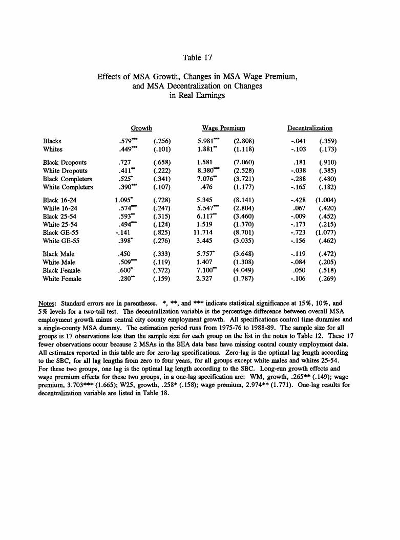
Table 17

Effects of MSA Growth, Changes in MSA Wage Premium,and MSA Decentralization on Changes

in Real Earnings

Growth Wage Premium Decentralization

Blacks Whites

Black Dropouts White Dropouts Black Completers White Completers

Black 16-24 White 16-24 Black 25-54 White 25-54 Black GE-55 White GE-55

Black Male White Male Black Female White Female

.579"

.449*"

.727

.4ir.525*

.390**

1.095* .574** .593~ .494**

-.141 .398*

.450 .509**

.600*

.280**

(.256) (.101)

(.658) (.222) (.341) (.107)

(.728) (.247) (.315) (.124) (.825) (.276)

(.333) (.119) (.372) (.159)

5.981***1.881**

1.5818.380***7.076**

.476

5.3455.547***6.117**1.519

11.7143.445

5.757*1.4077.100**

2.327

(2.808)(1.118)

(7.060)(2.528)(3.721)(1.177)

(8.141)(2.804)(3.460)(1.370)(8.701)(3.035)

(3.648)(1.308)(4.049)(1.787)

-.041-.103

.181-.038-.288-.165

-.428.067

-.009-.173-.723-.156

-.119-.084.050

-.106

(.359)(.173)

(.910)(.385)(.480)(.182)

(1.004)(.420)(.452)(.215)

(1.077)(.462)

(.472)(.205)(.518)(.269)

Notes: Standard errors are in parentheses. *, **, and *** indicate statistical significance at 15%, 10%, and 5 % levels for a two-tail test. The decentralization variable is the percentage difference between overall MSA employment growth minus central city county employment growth. All specifications control time dummies and a single-county MSA dummy. The estimation period runs from 1975-76 to 1988-89. The sample size for all groups is 17 observations less than the sample size for each group on the list in the notes to Table 12. These 17 fewer observations occur because 2 MSAs in the BEA data base have missing central county employment data. All estimates reported in this table are for zero-lag specifications. Zero-lag is the optimal lag length according to the SBC, for all lag lengths from zero to four years, for all groups except white males and whites 25-54. For these two groups, one lag is the optimal lag length according to the SBC. Long-run growth effects and wage premium effects for these two groups, in a one-lag specification are: WM, growth, .265** (.149); wage premium, 3.703*** (1.665); W25, growth, .258* (.158); wage premium, 2.974** (1.771). One-lag results for decentralization variable are listed in Table 18.

Table 18

Short-Run and Long-Run Effects on Real Earnings of Decentralization in 1-Lag Specification

Short-Run Effect Long-Run Effect

Blacks -1.549" (.833) -.159 (.412)Whites -.611"* (.357) -.099 (.250)

Black Dropouts -3.736** (2.015) -.048 (1.073)White Dropouts -1.430** (0.817) .105 (.450)Black Completers -.822 (1.097) -.519 (.546)White Completers -.793*** (.359) -.161 (.205)

Black 16-24 -1.162 (2.392) -.073 (1.169)White 16-24 .824 (.904) .159 (.483)Black 25-54 -1.542* (1.039) -.240 (.518)White 25-54 -1.037*** (.427) -.120 (.245)Black GE-55 -3.040 (2.466) -.790 (1.212)White GE-55 -.309 (.916) -.350 (.531)

Black Male -1.940** (1.093) -.237 (.550)White Male -.575 (.402) -.118 (.232)Black Female -1.394 (1.156) .052 (.595)White Female -.597 (.569) .003 (.311)

Notes: Short-run effect is immediate effect on real earnings of a change in decentralization variable, and long- run effect is cumulative effect after 1 year of decentralization, in a specification with 1 lag in all economic development variables (growth, wage premium change, and decentralization). Specifications also control time dummies. Standard errors are in parentheses. *, **, and *** indicate statistical significance at 15%, 10%, and 5% levels for a 2-tail test. Number of MSA time period observations on which estimates are based are as follows: all white groups, 1186; B, 988; BD, 789; BC, 935; B16, 777; B25, 947; B55, 757; BM, 924; BF, 946.

93

A natural interpretation of this result is that the MS A labor market can adjust

relatively quickly, but not instantaneously, to within-MSA shifts in employment. One would

expect adjustments of labor supply within an MSA to be easier than adjustments of labor

supply across MSAs. But these within-MSA adjustments might still take some time,

particularly for less mobile groups such as blacks and high school dropouts, who are

concentrated in central cities.

A second interpretation is that the lack of long-term effects of decentralization is due

to the crude nature of the decentralization measure used here. Measures used in other

studies that are specific to the person's neighborhood, such as average journey-to-work times

in that neighborhood for jobs for which the person is qualified, are far better measures of

how job access affects the person.

VIII. Conclusion

This report's findings support a key theme of the demand-side view of black urban

poverty problems: local labor demand conditions significantly affect black economic success.

This demand-side view has been most prominently advocated by William Julius Wilson and

John Kasarda, although others such as Bluestone and Harrison (1982) have also suggested the

importance of demand-side conditions in explaining black economic problems. Although

cultural and psychological factors may affect black economic problems, as Lawrence Mead

and others contend, culture and psychology do not prevent poverty from being reduced when

the local economy improves.

94

But this report's findings suggest that the features of local demand that matter are

somewhat different than the features Wilson and Kasarda emphasize. Wilson and Kasarda

stress that black poverty problems are being worsened by manufacturing decline in central

cities. This report's findings suggest that the overall metropolitan economy is at least as

important as the movement of jobs from central cities to suburbs. The findings also suggest

why manufacturing decline may cause problems: manufacturing industries tend to be high

"wage premium" industries, paying well relative to the credentials required. Employment

declines in high wage premium industries, whether in manufacturing or services, seem to

play an important role in harming black earnings. Although some deindustrialization

researchers, such as Bluestone and Harrison (1982), have stressed the importance of an

industry's wage levels, Bluestone and Harrison's point has sometimes become lost in

subsequent discussion.

The report's findings suggest general directions for public policy but do not prove

the case for any specific policy program. Economic development policies that increase

metropolitan growth and attract high wage premium industries can provide important labor

market benefits for both white and black residents. But exactly which economic development

policies (tax abatements, technology development programs, general tax cuts, improvements

in local education, assistance to manufacturers for modernization and exporting, business

incubators, entrepreneurial training programs) work best to accomplish these goals is unclear.

National policies that seek to provide blacks with more high wage jobs can make a

substantial difference in reducing black poverty and increasing black economic success. But

which such black labor demand policies (local economic development policies, helping blacks

95

migrate to healthier metropolitan economies, enterprise zones, public service jobs, wage

subsidies for private employment for disadvantaged workers) will be most effective in

helping blacks per dollar spent is unclear. The general policy direction of trying to increase

demand for black labor in local economies is sound. But much more policy experimentation

and research needs to be done to determine how best to improve the local economic climate

facing blacks.

96

References

Amemiya, Takeshi. 1985. Advanced Econometrics. Cambridge, Mass: Harvard University Press.

Bartik, Timothy J. 1991. Who Benefits From State and Local Economic Development Policies? Kalamazoo, Mich.: W. E. Upjohn Institute for Employment Research.

______. 1990. "The Market Failure Approach to Regional Economic DevelopmentPolicy." Economic Development Quarterly 4 (4): 361-70.

Blanchard, Olivier Jean and Lawrence F. Katz, "Regional Evolutions," Brookings Papers on Economic Activity, 1:1992, pp. 1-75.

Bluestone, Barry and Bennett Harrison. 1982. The Deindustrialization of America: Plant Closings, Community Abandonment, and the Dismantling of Basic Industry. New York, NY: Basic Books, Inc.

Bound, John and Richard B. Freeman. 1992. "What Went Wrong? The Erosion ofRelative Earnings and Employment Among Young Black Men in the 1980s." The Quarterly Journal of Economics 107 (1): 201-32.

Bound, John and Harry J. Holzer. 1991. "Industrial Shifts, Skills Levels, and the Labor Market for White and Black Males." National Bureau of Economic Research Working Paper number 3715 (May).

Bound, John and George Johnson. 1992. "Changes in the Structure of Wages in the 1980's: An Evaluation of Alternative Explanations." American Economic Review 82 (3): 371-92.

Cain, Glen G. and Ross E. Finnie. 1990. "The Black-White Difference in YouthEmployment: Evidence for Demand-Side Factors." Journal of Labor Economics 8 (1, pt. 2): S364-95.

Cross, Rod (ed.). 1988. Unemployment, Hysteresis, and the Natural Rate Hypothesis. New York: Basil Blackwell.

Dickens, William and Lawrence Katz. 1987. "Inter-Industry Wage Differences and Industry Characteristics." In Unemployment and the Structure of Labor Markets, eds. Kevin Lang and Jonathan S. Leonard. New York: Basil Blackwell.

97

Eggers, Mitchell L. and Douglas S. Massey. 1992. "A Longitudinal Analysis of Urban Poverty: Blacks in U.S. Metropolitan Areas between 1970 and 1980." Social Science Research 21, 175-203.

______. 1991. "The Structural Determinants of Urban Poverty: A Comparison ofWhites, Blacks, and Hispanics." Social Science Research 20, 216-55.

Ellwood, David T. 1986. "The Spatial Mismatch Hypothesis: Are There Teenage JobsMissing in the Ghetto?" In The Black Youth Employment Crisis, edited by Richard B. Freeman and Harry J. Holzer, 147-87. Chicago: University of Chicago Press.

Fleisher, B. and G. Rhodes. 1976. "Unemployment and the Labor Force Participation of Married Men and Women: A Simultaneous Model." Review of Economics and Statistics 58, 4 (November): 398-406.

Freeman, Richard B. 1991. "Employment and Earnings of Disadvantaged Young Men in a Labor Shortage Economy." In The Urban Underclass, edited by Christopher Jencks and Paul E. Peterson, 103-21. Washington, DC: The Brookings Institution.

______. 1989. "Labor Market Tightness and the Declining Economic Position ofYoung Less Educated Male Workers in the United States." Working Paper. Harvard University, December.

Frey, William H. and Alden Speare, Jr. 1988. Regional and Metropolitan Growth and Decline in the United States. New York: Russell Sage Foundation.

Geweke, John and Richard Meese. 1981. "Estimating Regression Models of Finite But Unknown Order." International Economic Review 22, 1 (February): 55-70.

Holzer, Harry J. 1991. "The Spatial Mismatch Hypothesis: What Has the Evidence Shown?" Urban Studies 28 (1): 105-22.

Houseman, Susan N. and Katharine G. Abraham. 1990. "Regional Labor Market Responses to Demand Shocks: A Comparison of the United States and West Germany." Paper presented at the Association for Public Policy Analysis and Management meetings in San Francisco, October 18-20.

Hughes, Mark Alan. 1989. "Misspeaking Truth to Power: A Geographical Perspective on the "Underclass" Fallacy." Economic Geography 65 (3): 187-207.

Ihlanfeldt, Keith R. 1992. Job Accessibility and the Employment and School Enrollment of Teenagers. Kalamazoo, MI: W. E. Upjohn Institute for Employment Research.

98

Ihlanfeldt, Keith R. and David L. Sjoquist. 1991. "The Effect of Job Access on Black and White Youth Employment: A Cross-sectional Analysis." Urban Studies 28 (2): 255- 65.

______. 1990. "Job Accessibility and Racial Differences in Youth EmploymentRates." American Economic Review 80: 267-76.

______. 1989. "The Impact of Job Decentralization on the Economic Welfare of Central City Blacks." Journal of Urban Economics 26, 110-30.

Jargowsky, Paul A. and Mary Jo Bane. 1991. "Ghetto Poverty in the United States, 1970- 1980." In The Urban Underclass, edited by Christopher Jencks and Paul E. Peterson, 235-73. Washington, DC: The Brookings Institution.

Juhn, Chinhui. 1992. "Decline of Male Labor Market Participation: The Role of Declining Market Opportunities." The Quarterly Journal of Economics 107 (1): 79-121.

Kasarda, John D. 1990. "City Jobs and Residents on a Collision Course: The Urban Underclass Dilemma." Economic Development Quarterly 4 (4): 313-19.

______. 1989. "Urban Industrial Transition and the Underclass." The Annals of theAmerican Academy of Political and Social Science 501: 26-47.

______. 1985. "Urban Change and Minority Opportunities." In The New Urban Reality, edited by Paul E. Peterson, 33-67. Washington, DC: The Brookings Institution.

Katz, Lawrence F. and Kevin M. Murphy. 1992. "Changes in Relative Wages, 1963-1987: Supply and Demand Factors." The Quarterly Journal of Economics 107 (1): 35-78.

Katz, Lawrence and Lawrence Summers. 1989. "Industry Rents: Evidence andImplications." Brookings Papers on Economic Activity (Microeconomics issue): 209- 90.

Kennedy, Peter. 1992. A Guide to Econometrics. (Third Edition) Cambridge, Mass.: The MIT Press.

______. 1986. "Interpreting Dummy Variables." Review of Economics and Statistics68: 174-75.

Krueger, Alan B. and Lawrence H. Summers. 1988. "Efficiency Wages and the Inter- Industry Wage Structure." Econometrica 56 (2): 259-93.

99

Leonard, Jonathan S., 1986. "The Spatial Mismatch Hypothesis: Are There Teenage Jobs Missing in the Ghetto." In The Black Youth Employment Crisis, edited by Richard B. Freeman and Harry J. Holzer, 185-90. Chicago: University of Chicago Press.

Levy, Frank. 1982. "Migration's Impact on the Economic Situation of Minorities and the Disadvantaged." Final Report, prepared under HUD Contract HC-6065. Washington, DC: The Urban Institute.

Marston, Stephen T. 1985. "Two Views of the Geographic Distribution ofUnemployment." Quarterly Journal of Economics 100 (February): 57-79.

Massey, Douglas S., Mitchell L. Eggers and Nancy A. Denton. 1990. "Disentangling the Causes of Concentrated Poverty." NORC/University of Chicago, Population Research Center Discussion Paper Number OSC 90-5 (May).

Mead, Lawrence M. 1992. The New Politics of Poverty: The Nonworking Poor in America. New York: Basic Books.

Mooney, J. 1969. "Housing Segregation, Negro Employment, and MetropolitanDecentralization: An Alternative Perspective." The Quarterly Journal of Economics 83: 299-311.

Moore, Thomas S. and Aaron Laramore. 1990. "Industrial Change and Urban Joblessness: An Assessment of the Mismatch Hypothesis." Urban Affairs Quarterly 25 (4): 640- 58.

Moss, Philip and Chris Tilly. 1991. "Why Black Men Are Doing Worse in the LaborMarket: A Review of Supply-Side and Demand-Side Explanations." Working paper prepared for the Social Science Research Council Subcommittee on Joblessness and the Underclass.

Moulton, Brent R. 1990. "An Illustration of a Pitfall in Estimating the Effects of Aggregate Variables on Micro Units." The Review of Economics and Statistics 72, 2 (May)" 334-38.

. 1988. "Using SAS to Estimate a Regression with Two Variance Components."Working Paper. Division of Price and Index Number Research, U.S. Bureau of Labor Statistics, April.

______. 1986. "Random Group Effects and( the Precision of Regression Estimates." Journal of Econometrics 32: 385-97.

Moulton, Brent R. and William C. Randolph. 1989. "Alternative Tests of the Error Components Model." Econometrica 57, 3 (May): 685-93.

100

Murphy, Kevin M. and Finis Welch. 1990. "Empirical Age-Earnings Profiles." Journal of Labor Economics 8, 2 (April): 202-29.

Osterman, Paul. 1991. "Gains from Growth? The Impact of Full Employment on Poverty in Boston." In The Urban Underclass, edited by Christopher Jencks and Paul E. Peterson, 122-34. Washington, DC: The Brookings Institution.

Roback, Jennifer. 1982. "Wages,Rents and the Quality of Life." Journal of Political Economy 90: 1257-78.

Rosen, Sherwin. 1979. "Wage-Based Indexes of Urban Quality of Life." In Current Issues in Urban Economics, eds. P. Mieszkowski and M. Straszheim. Baltimore: Johns Hopkins University Press.

Sherwood, Mark K. 1975. "Family Budgets and Geographic Differences in Price Levels." Monthly Labor Review 98, 4 (April): 8-15.

Suits, D. 1984. "Dummy Variables: Mechanics vs. Interpretation." Review of Economics and Statistics 66: 177-80.

U.S. Bureau of the Census. 1991. "Current Population Reports, Series P-60, No. 172."Money Income of Households, Families, and Persons in the United States: 1988 and 1989. Washington, DC: U.S. Government Printing Office.

Welch, Finis. 1990. "The Employment of Black Men." Journal of Labor Economics 8 (1, pt. 2): S26-S74.

White, H. 1980. "A Heteroskedasticity-Consistent Covariance Matrix Estimator and a Direct Test for Heteroskedasticity." Econometrica 48: 817-38.

Wilson, William Julius. 1987. The Truly Disadvantaged: The Inner City, the Underclass, and Public Policy. Chicago: The University of Chicago Press.

Winnick, Louis. 1966. "Place Prosperity vs. People Prosperity: Welfare Considerations in the Geographic Redistribution of Economic Activity." In Essays in Urban Land Economics in Honor of the Sixty-Fifth Birthday of Leo Grebler. Los Angeles: Real Estate Research Program, University of California at Los Angeles.

T-l

TECHNICAL APPENDIX

This technical appendix fills in details about the methodology and data of the report

Economic Development and Black Economic Success. The appendix is divided into three

main sections with several sub-sections. Section 1 discusses the estimation methodology.

Section 2 discusses the regression-adjusted estimated economic outcome variables (dependent

variables). Section 3 provides more detail on the economic development variables that are

constructed using two-digit industry data.

1. Details on the Estimation Methodology

Dependent Variable Definitions

Most dependent variables analyzed in this report are the percentage change in MSA

average economic outcomes for different groups from year t - 1 to year t. But calculating

percentage change is problematic if an economic outcome variable is nonpositive in either

year t or year t -1. For example, if percentage change is calculated as 100 times the change

in the natural logarithm, the natural logarithm is undefined at non-positive values of the

economic outcome variables. If percentage change is calculated using year t -1 values as a

base, the percentage change number will be infinite if the economic outcome variable has a

zero value in year t -1, and will have an unexpected sign if the economic outcome variable

has a negative value in year t -1. Even if economic outcome variables for year t or year

T-2

t - 1 are positive, percentage change numbers can be large if the positive numbers for year t

- 1 or year t are small. These large percentage change numbers could unduly influence

regression estimates.

For many MSA-year cases, this project's economic outcome variables are zero,

negative, or a small positive number. These problematic cases arise because particular

demographic groups often have a small sample size in a particular MSA and year. For

example, it might be that all black high school dropouts interviewed in Kalamazoo in 1988

happened to have zero earnings. Negative numbers can arise for earnings or wages because

this study includes self-employment earnings, which can be negative. In addition, the

regression adjustment procedure can produce negative predictions for economic outcomes in

an MSA for some group. Negative predictions would occur if a group has surprisingly low

values of the economic outcomes relative to the group's educational and experience

credentials. It is theoretically feasible to constrain the regression adjustment procedure to

prevent negative outcomes (for example, some type of tobit procedure). But such elaborate

statistical constraints would be prohibitively expensive in time given all the groups and

economic outcomes considered in this project.

To avoid these problems, percentage change in each economic outcome variable was

simply defined as the absolute change in that variable in that MSA from year t - 1 to year t,

divided by the sample mean over all MSAs and years in that variable, times 100, or

where ymgt is the mean value of some economic outcome for group g in MSA m in year r,

and yg is the mean value of that same economic outcome over all MSAs and years. This

T-3

definition is equivalent to estimating a model with absolute change in the economic outcome

variable as a dependent variable, and then multiplying all estimated coefficients by 100 over

the mean of the economic outcome variable to get percentage effects.

One objection to this procedure is that these percentage change values will go up or

down over time depending on the generally prevailing level of the economic outcome

variable in the nation. Perhaps this could bias estimates if the economic development

variables show some time trend. But all the estimating equations include a complete set of

dummy variables for time periods. These time period dummies should absorb any systematic

changes in percentage change values over time. In addition, the dependent variables are all

defined in real terms. There is often no clear time trend in the real level of the economic

outcome variables.

Heteroskedasticity

The report's main task is to estimate equations with the year-to-year percentage

change in MSA average economic outcome variables as dependent variables and the

percentage change in MSA "economic development" variables as independent variables. One

problem in estimating these equations is that their dependent variables are probably

heteroskedastic. The regression-adjusted MSA average economic outcome variables are

derived from the Current Population Survey. The CPS sample size varies a great deal from

one MSA to another. Because the sample size is small for some MSAs and large for others,

the error in measuring these regression-adjusted group means will be quite large in small

sample size MSAs and much smaller in large MSAs. This variation in measurement error

T-4

should create considerable heteroskedasticity in the year-to-year changes in the economic

outcome variable. Without some correction, this heteroskedasticity will make the coefficient

estimates less efficient, and will bias the estimated standard errors.

Any correction for this heteroskedasticity problem must consider the time and

complexity costs of imposing this correction on the many models estimated in this project. A

correction that is reasonably simple to simultaneously impose on many models has great

appeal.

A reasonably simple heteroskedasticity correction can be developed if we make some

simplifying assumptions that are literally false but likely to be approximately true. Suppose

that the dependent variable, instead of being the percentage change in the regression-adjusted

mean for MSA m from time t - 1 to time t, was instead the percentage change in the

ordinary mean. Assume further that the overall mean for the group (yg above) is accurately

enough estimated to be treated as non-stochastic. Assume further that the only source of

error in the estimating equation is the measurement error in measuring the group means for

the MSA for years t - 1 and t. Finally, assume that this measurement error is uncorrelated

between years t - 1 and t.

Under all these assumptions, the variance in the disturbance term in a typical

estimating equation can be written as the following equation:

(T- 2) n<w) •

where emgl is the disturbance term from the estimating equation in section III of the report's

main text, a2 is the variance of observations on the outcome variable for an individual

person, and Ngmt is the sample size for group g in MSA m in year /. Heteroskedasticity can

T-5

then be corrected by weighting all variables involved with a given group's outcome by 1 over

the square root of the term in brackets in equation (T.2). This term in brackets varies from

observation to observation only due to the sample size in years t - 1 and t for that group and

MSA. This same weighting will be used for a particular group, MSA, and year, regardless

of the dependent variables and independent variables in a particular specification. Because

reweighting is not required if the specification changes, more specifications can be tested in

less time.

This heteroskedasticity correction is literally false in several ways. But this correction

is still likely to provide a good approximate correction. The measurement error for

regression-adjustment means will not follow exactly the formula given in equation (T.2). But

this measurement error should strongly depend on the cell size in that MSA for those two

years, as (T.2) suggests. There is some correlation over time in the CPS measurement error,

as some households are included in the sample in two consecutive years. But this correlation

is likely to be roughly proportional to the term in brackets, so the same measurement error

variance will likely apply. 1 Finally, because of other sources of error in the estimating

equation, the disturbance term variance actually should equal a constant term plus some slope

coefficient times the bracket term in equation (T.2). But this bracket/measurement error

1 For example, when the sample size for the MSA and group is the same in both years, and exactly half of the CPS sample is retained from year to year (the extreme case), then the covariance between the measurement error will be given by

(l/2)po2 [l/Ay

where p is the year to year correlation in the economic outcome variable for the typical person in the sample both years.

T-6

variance is likely to be quite large compared to other sources of error. Also, as Kennedy

(1992, p. 131) has pointed out, attempts to estimate the disturbance term variance as a linear

function of the bracket term are likely to yield extremely imprecise estimates of the intercept

and slope coefficient. Estimation procedures will often be more efficient if they ignore the

other sources of disturbance variance.

Thus, there are some good arguments that this simple heteroskedasticity correction

will not be a bad approximation. Just as important, any of these possible "improvements" in

estimating the heteroskedasticity would tremendously complicate the estimation procedure for

all these many models, groups and variables. These more complicated procedures would not

necessarily improve the efficiency of the estimates.

Table Tl reports White heteroskedasticity tests and standard error corrections for the

black and white personal earnings models (White, 1980). These tests and corrections use

variables that have already been weighted and transformed, using the simple approximation

procedure implied by equation (T.I). This weighting is intended to eliminate

heteroskedasticity. In addition, after weighting, all variables were transformed to correct for

serial correlation. 2 Thus, these tests are examining whether there is any sign of significant

heteroskedasticity, which might affect the accuracy of our estimated standard errors, after

2 This estimated serial correlation is always negative. This negative serial correlation probably reflects measurement error again. Because ymgt.i enters negatively in %Aymgt , but positively in %Aymgt.ly the measurement error in y^^ will cause %Aymgt and %^ymgt-1 to be negatively correlated.

Table Tl

White's Test for Remaining Heteroskedasticity After Simple Heteroskedasticity Correction

Adjusted Real Personal Earnings Equation for Blacks

Adjusted Real Personal Earnings Equation for Whites

83.65

80.56

Standard errors for Estimated LR Effect of Growth

White's Chi- Squared Statistic df Probability

White-corrected Consistent

Standard errorOriginal Uncorrected

standard errors

79 .3388 .187 .185

74 .2815 .083 .074

Notes: Estimating equations are for zero-lag specification, with simple correction for heteroskedasticity and serial correlation.

T-8

doing our simple heteroskedasticity-serial correlation corrections. 3 The White test clearly

shows no sign of any remaining heteroskedasticity. Furthermore, heteroskedasticity

consistent standard errors do not differ much from the original standard errors.

Weighting Procedure for Comparing Estimates for One Group With the Estimates for Other Groups

A similar weighting procedure is used for regressions comparing results for one group

with results for some other group (e.g., black high school dropouts versus white high school

dropouts, and white high school dropouts versus white high school completers). These

comparison regressions examine whether an economic development variable such as MSA

employment growth has the same percentage effect on real earnings for two different

demographic groups. The comparison regressions use as a dependent variable the percentage

change in some economic outcome variable for one group (call it group r) minus the change

in some economic outcome for another group (group c). Suppose we continue to use the

same assumptions that were used to derive equation (T.2). In addition, assume that the

measurement errors for the two groups are uncorrelated. Under these assumptions, the error

variance for these "comparison regressions" will be given by the following equation:

3 The White test detects types of heteroskedasticity that are correlated with various products and cross-products of the independent variables in the model. It is these types of heteroskedasticity that affect the consistency of the package-produced standard errors (Kennedy, 1992, pp. 130, 131). Other types of heteroskedasticity may exist, and could allow for more efficient estimators, but these other types of heteroskedasticity will not cause the standard errors to be incorrect.

T-9

(T3) « , „„.,)] 1002+ d/5 c) » ! [WtfcJ + (W™,-,)] "CO2

Assume that the ratio of the standard deviation to the mean for each group is

approximately the same. It is plausible that this assumption is approximately true compared

to the tremendous variance in group sample size across MS As. Then the error variance for

these comparison regressions can be rewritten as the following equation:

.j) + (HNCM)

where* £ is some constant. To correct for heteroskedasticity, one over the square root of the

term in brackets is used to weight all variables for comparison regressions. The weighted

variables are then used in estimation with a first-order serial correlation correction.

Possible Biases in Standard Error Estimates Due to Pooling Cross-Section and Time-Series Data

The regression models of how economic development variables affect MSA economic

outcomes pool data across MS As and years. Such pooling of cross-section and time-series

data can bias the usual estimates of standard errors. The usual standard error calculations

assume that the disturbance is uncorrelated across different observations. But some

correlation across observations is often likely if cross-section and time-series data are pooled.

For the regression models of this report, the disturbance terms for the same year may be

correlated across different MSAs, and the disturbance terms for the same MSA may be

correlated across different years. If there is correlation across different observations in

disturbance terms, a new observation may not add as much new information as is assumed by

T-10

the simplest regression techniques. Hence, the true standard errors of the coefficient

estimates may be higher than the estimated standard errors that are provided using simple

regression techniques. These problems with pooling data have been extensively discussed in

the econometrics and labor economics literature by Moulton (1986, 1988, 1990), Moulton

and Randolph (1989), Freeman (1989, 1991), and Dickens and Katz (1987).

Any correlation in the disturbance across MSAs for a given year should be absorbed

by the year dummies included in all the regression equations. Any correlation in the

disturbance across years for a given MSA will be reduced because this project is analyzing

changes in economic outcomes in the MSA rather than the level of economic outcomes in the

MSA. Levels of economic outcomes in an MSA may be highly positively correlated because

unobserved attributes of the MSA—such as its amenities, city size, etc.—may heavily

influence wages and other economic outcomes in the city. But any unobserved attributes of

the MSA that are fixed over time disappear in a changes specification. In addition, the

regression estimation always corrects for the serial correlation that occurs between two

observations for adjacent years in the same MSA. This serial correlation correction could

potentially correct for any unobserved shocks that change economic outcomes in an MSA and

persist from year to year. As it turns out, however, the estimated serial correlation is always

negative. This negative serial correlation is probably due to measurement error in these

CPS-derived MSA regression-adjusted means. This measurement error-induced negative

serial correlation apparently overwhelms any positive serial correlation that might be caused

by persistent shocks to MSA economic outcomes.

T-ll

Despite this evidence, one could argue that there might be some significant positive

correlation in the disturbance term across non-adjacent years for the same MSA. This

positive correlation would bias usual standard error estimates. This positive correlation of

the disturbance within MSAs can be analyzed as being caused by unobserved "random

effects"—shocks to the disturbance term—that are MSA-specific and are part of the overall

disturbance term (Moulton, 1986, 1989, 1990). Moulton and Randolph suggest that the

presence of such random effects can be tested for using an F-test of whether a vector of

MSA "fixed effects"—dummy variables for each MSA—is statistically significant.4

I applied Moulton's F-test to two regressions: the regressions with percentage change

in overall black and white real earnings as dependent variables, and time dummies and

metropolitan employment growth as independent variables, with no lags in growth.5 These

F-tests clearly reject the hypothesis of unobserved MSA fixed or random effect components.

The relevant F-test statistic for blacks is .6047 (df=208, 1007; probability =.0000057). The

F-test for whites is .7347 (df=233, 1180; probability=.0017916). These F-tests show that

unobserved MSA effects do not significantly affect real earnings growth once we control

current MSA employment growth. Hence, there is no evidence that the standard error

4 Moulton and Randolph show that the traditional "Lagrange Multiplier" test for the presence of random effects is likely to be biased in most reasonably sized samples, and will too often reject the hypothesis of random effects.

5 This zero-lag model with only current growth and time dummies provides the maximum scope for any unobserved MSA effects to be present. Unobserved MSA effects are even less likely to be present if we add additional lags in growth, or add other MSA economic development variables to the specification.

T-12

estimates presented in this report are biased by unobserved correlations across observations

in different years for the same MSA. 6

2. Details on the Regression-Adjusted Economic Outcome Variables

Adjusting for Estimated Local Prices and Inflation

All estimated dollar amounts for average MSA economic outcomes are converted to

real terms using estimates of local prices and local inflation rates. This subsection describes

the procedures used for estimating local prices and local inflation rates.

For most of the economic outcome variables, it is only crucial to have good estimates

of local inflation rates, not local price levels. The dependent variables used in this report's

main estimating equations are the percentage change in MSA economic outcomes from year

to year. For variables such as personal earnings, or average earnings per week or per hour,

the real percentage change from year to year in the variable approximately equals the

nominal percentage change minus the local inflation rate.

But changes in the MSA poverty rate can not be expressed as simple function of the

inflation rate. Estimated local price levels will also make a difference in estimating poverty

rate changes.

6 In addition, the estimated effects of MSA growth in this zero-lag, MSA fixed effects specification are actually larger than are estimated without MSA fixed effects. The effects of a 1% shock to MSA employment on blacks in this fixed effects specification is 1.232 (standard error=.247); the effects on whites is .831 (.101). Hence, controlling for MSA fixed effects seems to tend to increase the estimated effects of employment growth on real earnings. However, it should be noted that controlling for MSA fixed effects may also tend to make the estimates more likely to represent short-run effects rather than long-run effects.

T-13

Unfortunately, the data on MS A inflation and prices are sparse. MS A inflation data

are consistently available only for the 1970s and 1980s for 24 MSAs.7' 8 MSA price level

data are only available for a few years in the 1970s, for around 38 MSAs. These MSA

"price level" data are three sets of U.S. Bureau of Labor Statistics' "living standard

budgets", showing how much it would cost in different MSAs to achieve an intermediate,

higher, and lower "standard of living."9

To estimate prices and inflation for MSAs and years for which data are not available,

I use the available MSA price and inflation data to make predictions. First, I estimate the

determinants of MSA price level differentials for 38 MSAs in 1976. The dependent variable

in this estimation is the BLS lower living standard budget for these 38 MSAs. The lower

living standard budget is chosen because the price level information is only needed for

7 Data are also available for part of this period for an additional MSA, Miami.

8 The U.S. Bureau of Labor Statistics reports these MSA numbers in the form of consumer price indices for different MSAs for different time periods, which might imply that these indices allow a comparison of price levels across MSAs. However, all these indices are arbitrarily set equal to 100 as of the same base year for all MSAs, so a comparison of indices across MSAs would really only show how much relative prices in different MSAs have changed since the base year. Also, the market basket used in different MSAs is different, and there is no attempt to ensure that the market baskets priced in different MSAs would yield the same level of utility or well-being.

9 These MSA "living standard" budgets also price different market baskets in different MSAs. However, these market baskets are supposed to be what it costs to achieve the same standard of living, given variations in such factors as climate (more clothes are needed to reach the same living standard in cold MSAs) and customs (certain foods are consumed more in some MSAs than others). These different market baskets could be seen as an ad hoc attempt to calculate the minimum cost needed to achieve a given utility level, and this attempt, if successful, would constitute a true cost of living index. Many economists might prefer a less ambitious but less ad hoc procedure of just pricing the identical market basket in different MSAs. But analysis of the intermediate living standard budget does not reveal any major changes in relative living costs when a fixed market basket is substituted for the MSA- differentiated market baskets. (Sherwood, 1975).

T-14

calculating poverty rates. The lower living standard budget will probably better approximate

the prices facing persons near the poverty line than will the intermediate or higher living

standard budgets. The estimates of the determinants of MSA "lower living standard" prices

are then used to predict relative price levels as of 1976 for all other MSAs. Second, I

estimate the determinants of MSA inflation differentials during the 1970s and 1980s for 24

MSAs. This estimated relationship is used to predict inflation rates for the other MSAs for

each year during the 1970s and 1980s. In both the price and inflation estimation, the goal of

the estimation is not to produce a full structural model of MSA prices or inflation. Instead,

the goal is an equation that will yield good out-of-sample predictions. Finally, I combine

these price level estimates for 1976 and inflation estimates for all years to generate a

predicted MSA price level for each year and each MSA.

Once these predictions are done, real poverty rates and real economic outcomes can

be calculated for each year and each MSA. This study's main dependent variables—the year-

to-year percentage change in MSA real economic outcomes and the change in the MSA

poverty rate—can then be calculated. All these calculations use actual data for local prices

and inflation when such data are available, and predicted values for prices and inflation when

the actual values are unavailable.

Table T2 reports the estimated determinants of 1976 MSA price level differentials.

The regional dummies simply reflect the well-known price level differences in different

regions of the country. The education variable is the average educational requirements in the

MSA implied by its 1976 industry mix, which might affect local wages and prices. This

particular specification was chosen over specifications that also included the MSA's size

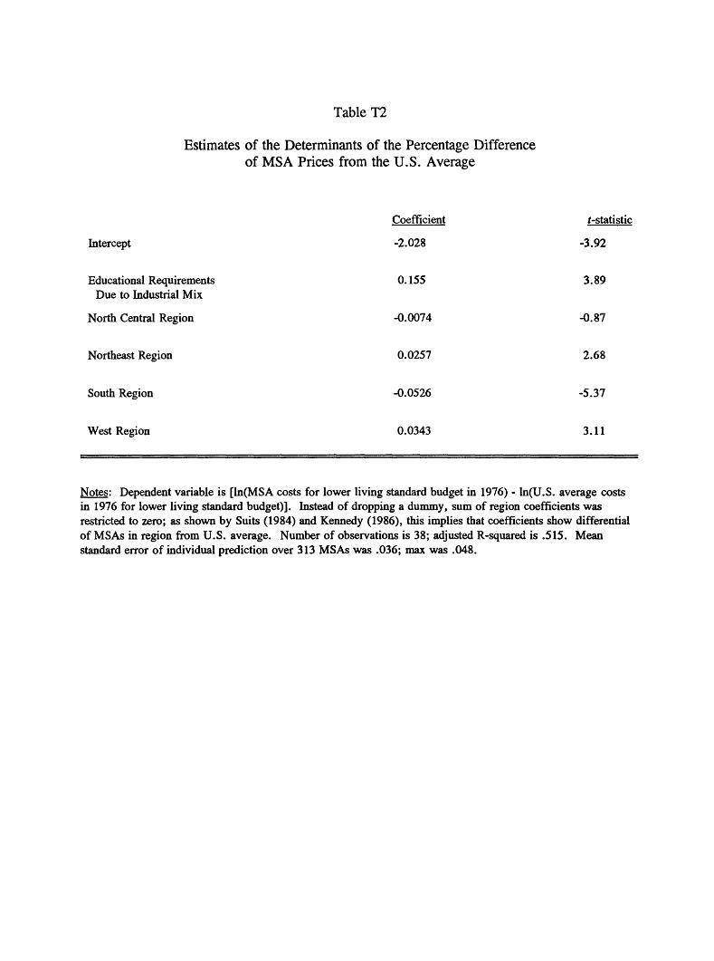
Table T2

Estimates of the Determinants of the Percentage Difference of MS A Prices from the U.S. Average

Intercept

Educational Requirements Due to Industrial Mix

North Central Region

Northeast Region

South Region

West Region

Coefficient

-2.028

0.155

-0.0074

0.0257

-0.0526

0.0343

f-statistic

-3.92

3.89

-0.87

2.68

-5.37

3.11

Notes: Dependent variable is [ln(MSA costs for lower living standard budget in 1976) - ln(U.S. average costs in 1976 for lower living standard budget)]. Instead of dropping a dummy, sum of region coefficients was restricted to zero; as shown by Suits (1984) and Kennedy (1986), this implies that coefficients show differential of MSAs in region from U.S. average. Number of observations is 38; adjusted R-squared is .515. Mean standard error of individual prediction over 313 MSAs was .036; max was .048.

T-16

(measured by employment) and the MSA's average wage premium. The chosen specification

was better than these alternatives according to the Akaike Information Criterion. The Akaike

Information Criterion is a standard model selection criterion that attempts to minimize the

out-of-sample prediction error, which is accomplished by excluding variables whose

estimated coefficients are too uncertain. 10 The resulting specification has a reasonably

adequate R-squared for a cross-section equation. The average estimated standard error of the

predictions is 3.6%. This standard error implies a 95% probability for the typical MS A that

the prediction is within 7.2% of the true relative price level.

For inflation, two prediction equations were constructed for two different time

periods, due to differences over time in available data. For the time period from 1971-72

through 1976-77, inflation determinants were estimated using the equation reported in Table

T3. Time period dummies reflect how MS A inflation is affected by national factors, and the

regional inflation variable reflects how MSA inflation is affected by regional factors. MSA

employment growth may affect MSA inflation by increasing local land and housing prices

and wages. Using the AIC, I chose this specification over a specification that also included

the change in the MSA manufacturing share. This equation has a quite high R-squared and

many highly significant right-hand side variables. More important, the equation yields a

quite small average standard error of individual predictions of .6%. This standard error

implies that for the average MSA-year observation, the inflation prediction has a 95% chance

of being within 1.2% of the true MSA inflation rate for that year.

10 As pointed out in Amemiya (1985), the AIC is virtually identical to his Prediction Criterion, which explicitly is designed to minimize out-of-sample prediction error.

Table T3

Estimates of Determinants of MSA Inflation 1971-72 to 1976-77

Intercept

1972 Dummy

1973 Dummy

1974 Dummy

1975 Dummy

1976 Dummy

1977 Dummy

Region's Inflation

MSA Employment Growth

Lagged MSA Growth

Twice Lagged Growth

Coefficient

0.03807

-0.02180

-0.00494

0.01793

0.00968

-0.00771

Excluded

0.427

0.05140

-0.00132

0.05847

f-statistic

5.34

-5.30

-2.58

3.57

2.41

-2.59

Excluded

3.93

1.33

-0.03

1.61

Notes: Inflation measured as [ln(MSA price index in year f) - ln(MSA price index in year t-1)]. Region's inflation is rate for the region MSA is in (4 regions report inflation rates, Northeast, North Central, South, and West). MSA Employment Growth is ln(MSA employment in year f) - ln(MSA Employment in year t-1). Lags are this variable one and two years ago. Number of observations is 144, Adjusted R-squared is .936. Mean standard error of individual predictions is .0064; max is .0093.

T-18

For the time period from 1977-78 through 1988-89, I estimated MSA inflation

determinants using the equation reported in table T4. This equation includes the same

independent variables as in the inflation prediction equation reported in table T3. The

additional independent variables in table T4 include current and lagged changes in

educational requirements. According to the AIC, this specification was superior to alternative

specifications that included changes in the MSA wage premium, changes in the MSA's

manufacturing share, and changes in other MSA "demographic share" economic development

variables. Why increases in the MSA educational requirements variable are associated with

lower MSA inflation is unclear. Perhaps increases in educational requirements over time

may contribute to reduced wages in some local retail industries that as a result have an

excess supply of workers. Alternatively, perhaps higher education industries are attracted to

MS As with lower inflation rates. Whatever the reason, the resulting specification again has a

quite high R-squared, and a low average standard error of prediction.

After these estimates were used to construct initial price level estimates for all MSAs

for all years, as described above, two additional adjustments were made. First, all the MSA

indices were multiplied by a constant to ensure that the employment-weighted average MSA

price index for 1989 is 100; that is, all indices were adjusted so that all nominal dollar

amounts will be measured in 1989 "average MSA" dollars. Second, MSA prices in 1982 and

previous years were multiplied by a year-specific but MSA-invariant factor, equal to the ratio

of the CPI-U-X1 price index for that year in the nation to the ordinary CPI-U index for the

nation for that year. The CPI-U official price index prior to 1983 is often argued to have

overestimated overall inflation because of problems in its calculation and treatment of

Table T4

Estimates of Determinants of MSA Inflation 1977-78 to 1988-89

Intercept

1978 Dummy

1979 Dummy

1980 Dummy

1981 Dummy

1982 Dummy

1983 Dummy

1984 Dummy

1985 Dummy

1986 Dummy

1987 Dummy

1988 Dummy

1989 Dummy

Region's Inflation

MSA Employment Growth

Lagged MSA Growth

Twice Lagged Growth

Change in MSA Educational Requirements

Lagged Change in Educational Requirements

Twice Lagged Change in Educational Requirements

Notes; Change in educational requirements

Coefficient

0.00581

0.01268

0.01836

0.02238

0.01899

0.01010

0.01401

0.00853

0.00108

-0.00742

0.00076

0.00306

Excluded

0.765

-0.11465

0.13333

0.07012

-0.17628

-0.06664

-0.14026

is the economic development variable

f-statistic

1.01

2.81

2.61

2.45

2.96

2.80

3.77

2.27

0.28

-1.64

0.23

0.97

Excluded

7.27

-1.98

1.92

1.29

-1.54

-0.59

-1.30

described in Table 3 of text.Number of observations is 299. Adjusted R-squared is .913. Mean standard error of individual predictions is .0114; max is .0169.

T-20

housing prices. The CPI-U-X1 is an unofficial index prepared by BLS that attempts to

correct for these problems in the treatment of inflation in the 1970s and 1980s. A more

sophisticated version of the CPI-U-X1 became the official CPI-U price index in 1983.

Hence, this correction attempts to at least roughly avoid over-estimating the inflation rate,

and thus underestimating improvements in poverty, during the 1970s and early 1980s.

Choice of Control Variables for Regression Adjustment Procedure

The purpose of the regression adjustment procedure is to accurately predict—for each

demographic group, MSA, and year—the value of each economic outcome for a person with

"standard" characteristics. As described in the text, these "standard" characteristics are

average characteristics for blacks as of the March 1987 CPS. These predictions are

"regression-adjusted" means. Regression-adjusted mean values of economic outcomes are

preferable to ordinary MSA mean values of economic outcomes because they are more

comparable across MSAs and over time. Adjusted means compare persons with the same

characteristics, whereas ordinary means may be unusually high or low because of an unusual

mix of persons in the MSA in that year.

A good prediction must use a regression specification that is complete and includes

only right-hand side variables whose effets are statistically significant at some minimum level

of significance. The regression specification must capture the relevant characteristics of

persons that explain economic outcomes. Yet if the specification includes too many variables

that are statistically insignificant, the resulting predictions will have high standard errors.

T-21

I initially considered estimating a separate regression equation for each year, MS A,

economic outcome, and demographic group. But preliminary experiments showed that this

approach resulted in adjusted means with unacceptably high standard errors. Many MSAs

have small samples in the Current Population Survey. Allowing regression coefficients to

vary by MSA resulted in imprecise estimates of the regression coefficients and therefore

imprecise predictions of the economic outcomes for persons with "standard" characteristics.

Instead, I estimated a specification, for each year, economic outcome, and

demographic group, that used an economic outcome as a dependent variable, and the

following types of independent variables: MSA dummies, and selected personal

characteristic variables. This specification allows the average level of the economic outcome

to vary by MSA. But the effects of the personal characteristic variables are constrained to be

the same in all MSAs. Although this constraint is unlikely to be literally true, imposing it

reduces the standard error of the predictions. Separate regressions were run for each year,

and demographic group, so coefficients were allowed to vary from year to year and over

different demographic groups.

The personal characteristics used as independent variables were a dummy variable for

gender, a dummy variable for high school completion, years of education completed, years

of education squared and cubed, age, and powers of age up to the fifth power. This

specification was selected after some experimentation. This experimentation concentrated on

picking a model that would be a good specification for black personal earnings. All these

variables are statistically significant for blacks overall. Furthermore, plots of the residuals

by age or education level do not reveal any important age or education groups for which this

T-22

specification tends to overpredict or underpredict earnings for blacks. The number of powers

used in age may seem high to some readers, but recent research suggests that labor

economists have often used too few powers in age or experience to accurately capture age-

earnings profiles (Murphy and Welch, 1990).

Table T5 summarizes the results from a typical regression used to calculate the

adjusted means. This particular regression is for blacks overall, for the year 1986. As can

be seen in the table, all the variables are statistically significant.

One possible criticism of this regression adjustment procedure is that it restricts the

effect of age, education, or gender on earnings to be the same in all MSAs. This criticism is

valid for the calculation of regression adjusted means for blacks overall or whites overall.

But this restriction is later relaxed because the report also analyzes changes in regression-

adjusted means for different subgroups of blacks and whites. Separate regression adjustment

procedures were done for each subgroup: two education groups (high school dropouts and

high school completers), three age groups (persons 16-24; 25-54; 55 and over), and both

genders. For each of these demographic subgroups for which this regression adjustment

procedure was done, a separate regression was run. Thus, all of these regressions'

coefficients, including the MSA dummies' coefficients, were allowed to vary between

demographic subgroups. Because the MSA dummies coefficients vary between subgroups,

different MSAs are allowed under this procedure to have different relative earnings for high

school dropouts versus completers, or for the three age groups considered, or for females

versus males.

Table T5

Effects of Personal Characteristics on Earnings for Blacks, 1986, with MSA Dummies Included

Intercept

EDUCATION

(EDUCATION)2

(EDUCATION)3

AGEAGE2

AGE3

AGE4

AGE5

GENDER DUMMY VARIABLE (FEMALE=1)

HIGH SCHOOL COMPLETION DUMMY VARIABLE (COMPLETIONS)

Notes; Personal earnings is dependent variable.

Coefficient

37837.4506

865.6525

-147.9815

8.7511

-7634.7681

400.9253

-8.7771

0.0846

-0.00030

-3774.2857

1344.2052

In addition to variables

/-statistic

3.44

2,21

-3.15

5.54

-8.64

9.92

-10.22

9.87

-9.21

-17.66

3.33

listed in this table, the regression alsoincluded as independent variables a complete set of MSA dummy variables. F-test for significance of MSA dummies: 2.03 (df=209; 6969); probability of F-test of this size when no true effect of MSA dummies is .0001. Adjusted R-squared = .383; Sample size = 7,189.

T-24

Calculation of Standard Errors for Late 1970s to Late 1980s Percentage Change in Real Earnings for Selected MSAs (Figure 3)

Figure 3 presented estimates of the percentage change in regression adjusted real

personal earnings for blacks and whites separately, in selected MSAs, from the late 1970s to

the late 1980s. This figure reported standard errors of these estimates. This subsection of

the technical appendix will outline how these standard errors were calculated. This

calculation is quite straightforward. There is but one complication: because some CPS

households remain in the CPS sample from one year to the next, the errors in estimating

MS A means for adjacent years are positively correlated.

The variance of these percentage change numbers is given by the following formula:

(T5) F[100(F8 -r7)/F7] «

Y7 is the average regression-adjusted real personal earnings for a particular MS A, either for

blacks or whites, for 1976, 1977, 1978, and 1979. This is a simple average, calculated as

the sum of the individual years' figures divided by four. Y8 is a similar average for 1986

through 1989. This variance calculation is an approximation relying on a Taylor-series

expansion.

The variance of the late 1970s average, 77, is given by the following formula:

T-25

(T.6)

+ \ [C(Y16,o

Y76 is the regression-adjusted mean personal earnings for blacks or whites in a particular

MS A in 1976, Y77 for 1977, etc. The formula assumes that the CPS sample is independent

in non-adjacent years, but may have some correlation in adjacent years. The CPS sampling

structure is such that half the housing units in the sample are replaced from one March to the

next, whereas the other half of the housing units interviewed are the same from one March to

the next. As a result, calculated statistics for adjacent years should have some correlation,

whereas statistics in non-adjacent years should not be correlated. A formula similar to

equation (T.6) applies to the variance of Y8.

I assume the following correlation among regression-adjusted means for adjacent

years:

The assumption of a year-to-year correlation of .30 relies on information from the Census

Bureau (U.S. Census Bureau, 1991, Table D-6 on p. 401). Strictly speaking, this correlation

of .30 only applies to unadjusted simple means for personal income figures. One would

think that the regression adjustment procedure should reduce the year-to-year correlation,

because the regression adjustment eliminates some of the sampling error that results from

happening to draw a sample with unusual personal characteristics. As a result, using

equation (T.7) may result in overstating the year to year correlation, and hence overstating

T-26

all the variances in equations (T.5) and (T.6). Thus, the reported standard errors in figure 3

may be a bit too high.

To calculate all these variances, I used SAS to calculate the variance of the

regression-adjusted means for each MSA, year, and group (blacks or whites) in the late

1970s and late 1980s. This variance depends on the variance-covariance matrix of the

coefficient estimates and the vector of standard characteristics used to calculate the

regression-adjusted means. These variances were then plugged into equations (T.7) and

(T.6), and then substituted into equation (T.5). The square root of these variance estimates

in equation (T.5) are reported as standard errors in Figure 3.

3. Details on the Construction and Use of the Economic Development Variables

Overcoming Suppressed 2-Digit Industries

Several of the MSA "economic development" variables depend on the MSA's industry

mix. Examples include the wage premium variable, the educational requirements variable,

and the variables measuring the share of MSA labor demand for the different demographic

groups. The calculation of these industry mix variables require data on employment by 2-

digit industries in the MSA for each year. But such 2-digit industry employment data are

frequently not available due to "data suppressions." For confidentiality reasons, federal

statistical agencies often will not release information for a particular 2-digit industry's

employment in a particular MSA and year.

I overcame these suppressions by estimating the employment in suppressed industries.

The procedure began by estimating suppressed 1-digit industries at the state level. The

T-27

procedure then went on to estimate in turn suppressed 2-digit industries at the state level,

suppressed 1-digit industries at the MSA level, and suppressed 2-digit industries at the MSA

level.

At each stage, an outline of the procedure is as follows. Suppressed industry

employment numbers for a particular geographic unit (state or MSA) and year were initially

estimated where possible by interpolating or extrapolating from reported numbers for that

same industry and geographic unit for other years. If interpolation or extrapolation was

impossible because that industry was suppressed in that geographic unit for all years, then the

industry's employment number was estimated by using information on the industry's share of

employment in that year in the next higher geographic unit (i.e., the U.S. for a state, or the

state for an MSA). These initial estimates were then adjusted upwards or downwards so the

sum of industry numbers for that state or MSA added up to the next broader industrial

category. That is, the initial 2-digit estimates would be adjusted so that all 2-digit industry

employment numbers would add up to the appropriate 1-digit totals for that geographic unit;

the initial 1-digit numbers would be adjusted so that they added up to the all-industry total

for that geographic unit.

The initial estimates from interpolation, extrapolation, or higher level geographic units

were developed using industry share numbers. Interpolation assumed a constant linear

change in an industry's share of the next higher level industrial categories between the

observed years. Thus, if a 2-digit industry's share in a geographic unit of its 1-digit category

was .15 in 1985 and .17 in 1987, with 1986 suppressed, the initial estimates assumed a .16

share for the industry in 1986. Extrapolation assumed a constant industry share of the next

T-28

highest industrial category from the nearest available year for that industry in that geographic

unit. Thus, if the last available year for a 2-digit industry had a share of .21 out of its 1-

digit category, I assumed that share would continue into the future. Alternatively, if the first

available year for a 2-digit industry had a share of .21, I assumed that its share was .21 in

previous years. Finally, if interpolation or extrapolation was not possible (because the

industry was suppressed for all years for that geographic unit), I assumed that the industry's

share of the next highest level industrial category was the same in the next highest level

geographic unit for which data were available. Thus, if a 2-digit industry was suppressed for

all years for an MS A, its share of the appropriate 1-digit total in that MS A was assumed to

be the same as the 2-digit share of the 1-digit total in the state in which the MS A was

primarily located.

I implemented this procedure using two different data bases. One data base was from

the Regional Economic Information System of the U.S. Bureau of Economic Analysis. This

data base provided 2-digit and 1-digit industry employment numbers for the nation and states,

and 1-digit numbers for MSAs, for all years from 1969 to 1989. These numbers are official

total full time and part time employment estimates prepared by BE A. The second data base

was "ES-202" data from the U.S. Bureau of Labor Statistics. This data base provided 2-digit

and 1-digit employment numbers for the nation, states, and MSAs, for all years from 1975 to

1989. These numbers are raw counts of the number of employees covered by unemployment

insurance. Both data bases use the same MSA definitions for all years, and the MSA

definitions are consistent between the 2 data bases.

T-29

The REIS data are probably overall better because they are estimates, whereas the

ES-202 data simply provides raw counts of employees covered. The ES-202 data are not

adjusted for changes in unemployment insurance coverage or reporting, or any other factors

that might affect the accuracy of the numbers. On the other hand, the ES-202 data base is

unique in providing annual average information at the 2-digit level of detail for MSAs.

Because of these different strengths and weaknesses of the two data bases, the REIS

data were used to provide all estimates of 1-digit employment numbers at the MSA level.

The ES-202 data was used to provide estimates of the 2-digit shares of 1-digit totals at the

MSA level. These ES-202 derived 2-digit shares were then applied to the REIS-derived 1-

digit employment numbers to get 2-digit employment numbers.

The actual procedure went as follows. First, REIS suppressions were overcome at

the state level, for 1-digit industries. Second, REIS suppressions were overcome at the MSA

level for 1-digit industries. Third, ES-202 suppressions were overcome at the MSA level for

1-digit industries. 11 Fourth, ES-202 suppressions were overcome at the MSA level for 2-

digit industries. Fifth, the 2-digit shares of 1-digit numbers from steps 3 and 4 were applied

to the 1-digit numbers from step 2 to get 2-digit numbers at the MSA level.

Although estimating the suppressed industries was quite time-consuming, it is

important to note that most industries were not suppressed. For the average MS A/year

combination, about 15 of the 73 2-digit industries were suppressed. For the average MSA,

less than 3 of the 73 2-digit industries were suppressed for all years from 1975 to 1989.

11 If interpolation or extrapolation was impossible, and state 1-digit or 2-digit numbers were suppressed for ES-202, national shares were used to obtain the initial estimates.

T-30

Hence, the "industry mix" economic development variables mostly use real industry

employment numbers rather than estimated numbers. Furthermore, even in cases where

estimates were made, these estimates are likely to be fairly good. It is not implausible to

assume that interpolating or extrapolating industry share numbers from other years for the

MS A, or using industry share numbers from the state, will give reasonably accurate industry

share numbers for the MS A.

Decomposition of Causes of Shifts in Black High School Completer and Black High School Dropout Labor Demand

Figures 5 and 6 in the main report show surprising trends in the percentage share of

labor demand for black high school dropouts and black high school completers. Figure 5

shows that black high school completer demand has declined over time. Figure 6 shows that

black high school dropout demand has increased over time.

The text discussion attributes these trends to various changes in the U.S. industrial

mix, and the particular industries in which black high school dropouts and completers are

concentrated. This subsection will back up the report's assertions with some data.

As defined in this report, the percentage of labor demand for black high school

dropout or completer demand as of some year r, for all MS As, can be expressed by the

following equation:

(T- 8) Bt = (1/100)2 7^.i

where Bt is the percentage of total MSA labor demand that we would expect to go to this

particular black group given the industry mix as of year t, BL is the percentage of

T-31

employment in industry i that goes to that particular black group according to the 1990

Current Population Survey, and Pit is the percentage share of that industry i in total

employment for all MSAs as of year t. This variable is a prediction of the percentage of

demand for that black group if each industry in the U.S. employed the same percentage of

that group as it did in the 1990 CPS.

The change from year s to year t in this black labor demand variable can be

decomposed by the following formula:

(T.9)Bt -Bs =

where B is the percentage share of employment in all industries that goes to the particular

black group being considered. The second equality in (T.9) follows because both Pit and P^

sum to 100 and B is a constant across all industries.

The decomposition in equation (T.9) is useful because it can be used to measure each

industry's "contribution" to the total change in labor demand for some black group. An

industry will make a positive contribution to increasing demand for a black group in either of

two cases: (1) the percentage share of total employment demand in that industry is

increasing (P,,-/^ is positive) and that black group has an above-average share of that

industry's employment (BrB is positive), or (2) the percentage share of total employment

demand in that industry is decreasing and that black group has a below-average share of that

industry's employment. Similarly, an industry will tend to be decreasing a black group's

labor demand in either of two cases: (1) it is a fast growth industry and that black group has

T-32

a below-average share of that industry, or (2) it is a slow growth industry and that black

group has an above-average share of that industry.

Tables T6 and T7 show a few of the key industries that contribute to the observed

trends in black high school dropout and completer demand from 1979 to 1989. Table T6

shows that black high school dropout demand was significantly boosted by the relatively fast

employment growth in the eating and drinking place industry and the private household

services industry. Black high school dropouts had above-average shares of the employment

in these two fast-growth industries. Other industrial changes tended to decrease black

dropout labor demand, but not by enough to fully offset the effects of these two industries'

growth.

Table T7 shows that black high school completer demand was significantly reduced

by relatively slow growth in government employment (both military and civilian, federal and

state and local) and communications industry employment. Black high school completers had

above-average shares of the employment in these slow-growth industries. Other industrial

changes did tend to increase black completer labor demand, but not by enough to offset these

declines in government and government-regulated industries.

Table T6

Decomposition of Components of Change in Black High School Drop-Outs Percentage Share of Labor Demand, 1979-89

(1) (2) (3) (4)Difference of Black Contribution of Industry

Change in Percentage High School Drop-Out to Change in BlackIndustry's Share, Percentage From All Drop-Out Share

Industry ___1979-89 Industry Average

Food products -4.05 4.20 -.0170

Eating & drinking places .618 2.76 .0170

Private household .129 12.38 .0160 services

All other industries -.0073

Total change in .0087percentage share of labor (from 2.2492demand to 2.2579%)

Notes: Column (2) is change in industry's percentage share of total employment, 1979 to 1989, for all MSAs. Column (3) is percentage of industry's employees who are black high school dropouts minus similar percentage for all industries.

Table T7

Decomposition of Components of Change in Black High School Completers Percentage Share of Labor Demand, 1979-89

(1) (2) (3) (4)Difference of Black Contribution of Industry

Change in Percentage High School Completer to Change in BlackIndustry's Share, Percentage From All Completers Share

Industry 1979-89 Industry Average 1(4)=[(3X2)1 • .01}

Federal civilian -.349 8.13 -.0284 employment

Federal military -.178 8.90 -.0158 employment

State and local -1.111 3.09 -.0343 government employment

Communications -.335 6.90 -.0231

All other industries .0113

Total change in -.0903 (frompercentage share of labor 8.3173% todemand, 1979-89 8.2270%)

Notes: Column (2) is change in industry's percentage share of total employment, 1979 to 1989, for all MSAs. Column (3) is percentage of industry's employees who are black high school completers minus similar percentage for all industries.