economic growth & development: part 2 horizontal

©Kiminori Matsuyama, Growth & Development Part-2

of 21

Economic Growth & Development: Part 2 Horizontal Innovation Models

By Kiminori Matsuyama

Updated on 2011-04-06, 6:00:49 PM


of 21

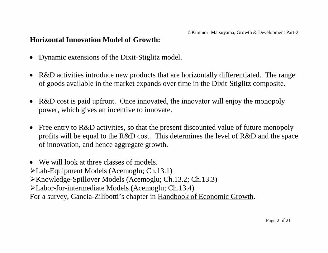
Horizontal Innovation Model of Growth: Dynamic extensions of the Dixit-Stiglitz model. R&D activities introduce new products that are horizontally differentiated. The range

of goods available in the market expands over time in the Dixit-Stiglitz composite. R&D cost is paid upfront. Once innovated, the innovator will enjoy the monopoly

power, which gives an incentive to innovate. Free entry to R&D activities, so that the present discounted value of future monopoly

profits will be equal to the R&D cost. This determines the level of R&D and the space of innovation, and hence aggregate growth.

We will look at three classes of models. Lab-Equipment Models (Acemoglu; Ch.13.1) Knowledge-Spillover Models (Acemoglu; Ch.13.2; Ch.13.3) Labor-for-intermediate Models (Acemoglu; Ch.13.4) For a survey, Gancia-Zilibotti’s chapter in Handbook of Economic Growth.


of 21

Lab-Equipment Model (Acemoglu Ch.13.1): The final good is used as the input to R&D activities, hence called “lab-equipment model.”

tN

Household

Final Goods Sector

R&D Sector Intermediate Inputs Sector

L Ct

Zt Xt xt(ν); 0 ≤ ν ≤ Nt


of 21

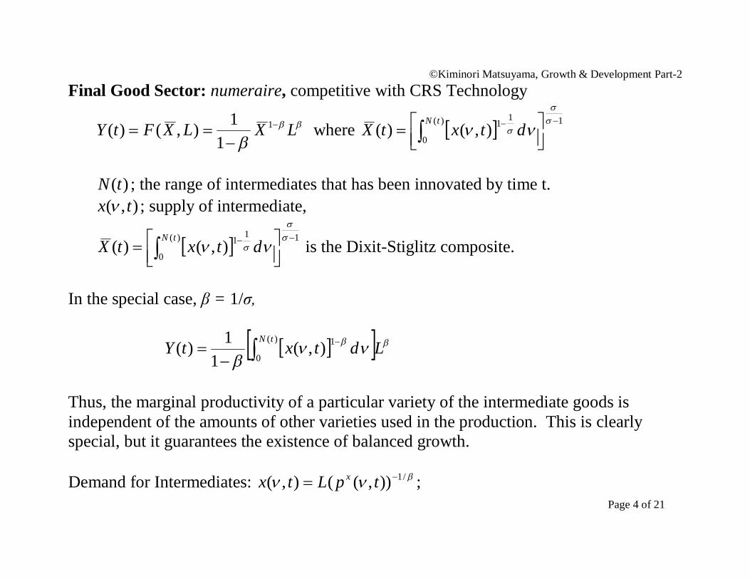
Final Good Sector: numeraire, competitive with CRS Technology

LXLXFtY

1

11),()( where 1)(

0

11),()(

tN

dtxtX

)(tN ; the range of intermediates that has been innovated by time t.

),( tx ; supply of intermediate,

1)(

0

11),()(

tN

dtxtX is the Dixit-Stiglitz composite.

In the special case, β = 1/σ,

LdtxtYtN

)(

0

1),(1

1)(

Thus, the marginal productivity of a particular variety of the intermediate goods is independent of the amounts of other varieties used in the production. This is clearly special, but it guarantees the existence of balanced growth. Demand for Intermediates: /1)),((),( tpLtx x ;


of 21

Intermediate Inputs Sector: Monopolistically competitive; N(t) firms, each producing its own variety as a sole producer units of the final good are required to produce one unit of output. By normalizing

1 , Monopoly Pricing: 1),()1)(,( tptp xx for all ν and t.

Ltx ),( and Lt ),( for all ν and t.

)(1

)( tNLtY

; )()1()( tLNtX ; )(1

)( tNtw

.

Note that the economy grows with )(tN .

Value of Intermediate Firm:

t

st dsduurstV )(exp)()(

This assumes that, once innovated, each product is forever produced by a monopolist. (Perpetual patent protection, for example.)

Differentiating with respect to t yields )()()( tVtrtV

.


of 21

Representative Household: supply L to earn the wage income, w(t)L, and invest in the

shares of the intermediate firms, VN

, to earn the profit income, N , and choose consumption of the final good, C, to:

Max 0

)( dtetCuU t

0

1

11)( dtetC t

, subject to

Flow Budget Constraint:

VNrNVwLNVrVwLNwLCVN )(

CwLNVrNV

)()(

)0()0()()(lim)0()0(])()([ 00)(

0

)(VNetVtNVNdteLtwtC

ttduur

t

duur

Intertemporal Budget Constraint:

0

00

0 )(exp)()0()0()(exp)( dtduurLtwVNdtduurtC tt

)(trCC ; 0exp)()(lim 0

tut durtVtN


of 21

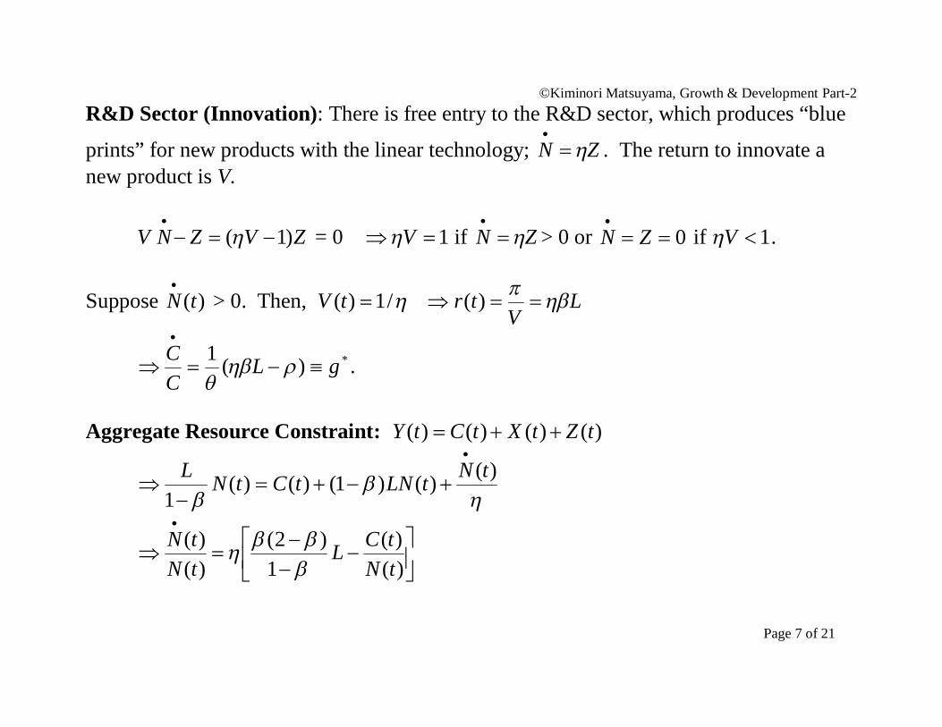
R&D Sector (Innovation): There is free entry to the R&D sector, which produces “blue

prints” for new products with the linear technology; ZN

. The return to innovate a new product is V.

ZVZNV )1(

= 0 1 V if ZN

> 0 or 0

ZN if 1V .

Suppose )(tN

> 0. Then, /1)( tV LV

tr )(

*)(1 gLCC

.

Aggregate Resource Constraint: )()()()( tZtXtCtY

)()()1()()(

1tNtLNtCtNL

)()(

1)2(

)()(

tNtCL

tNtN


of 21

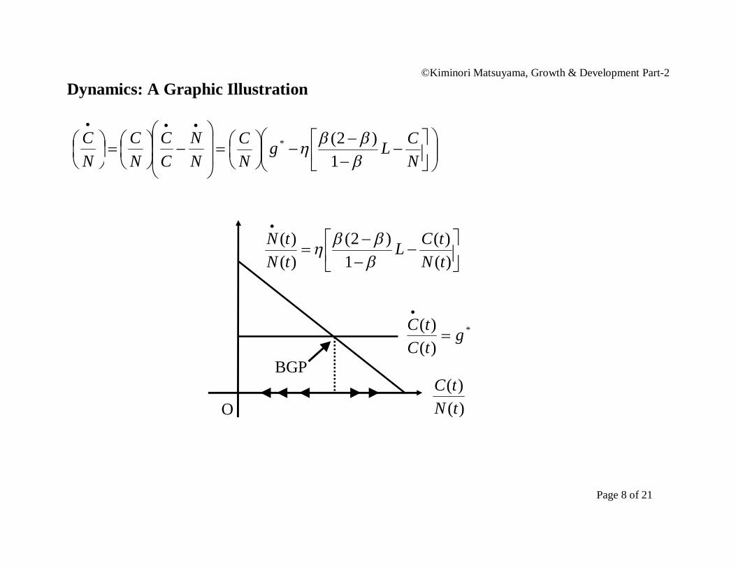
Dynamics: A Graphic Illustration

NC

NN

CC

NC

NCLg

NC

1)2(*

O

BGP

)()(

1)2(

)()(

tNtCL

tNtN

)()(

tNtC

*

)()( g

tCtC


of 21

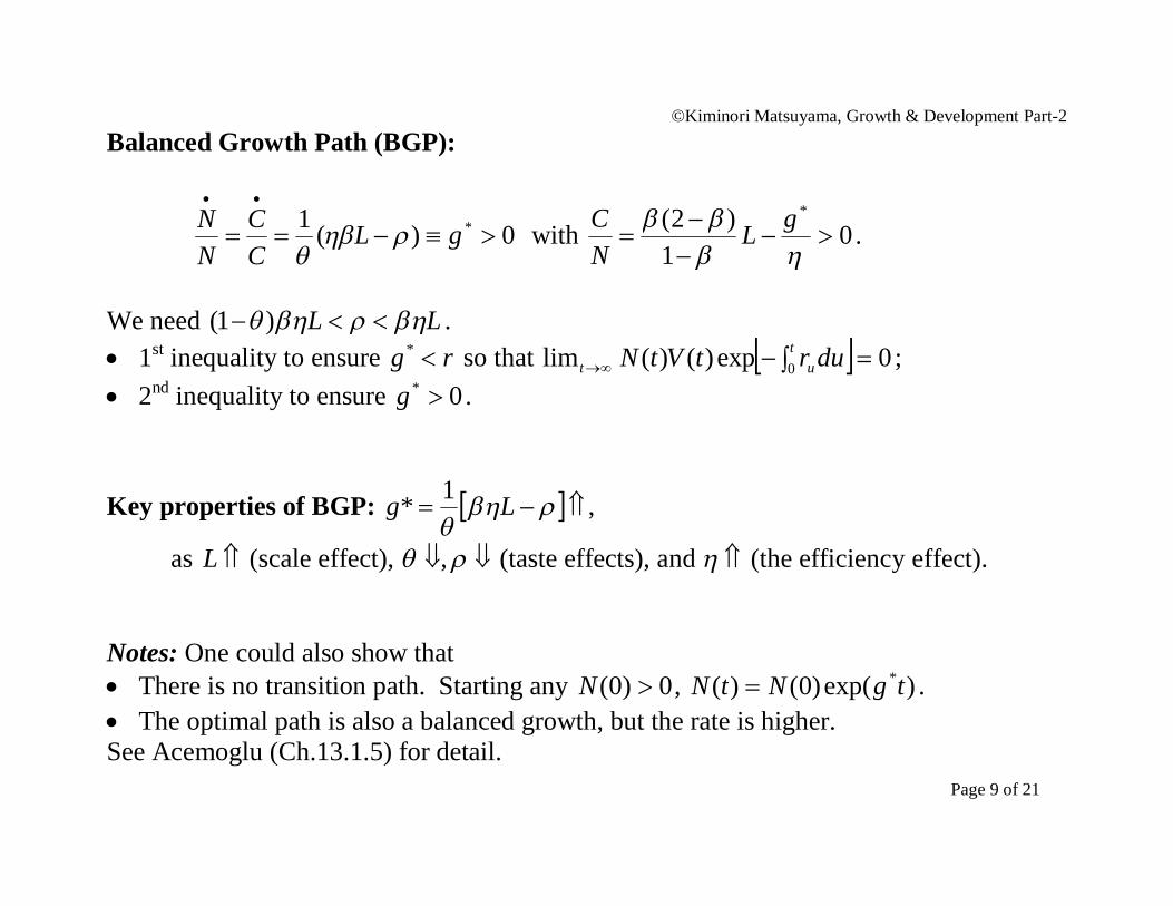
Balanced Growth Path (BGP):

0)(1 *

gLCC

NN

with 0

1)2( *

gLNC .

We need LL )1( . 1st inequality to ensure rg * so that 0exp)()(lim 0

tut durtVtN ;

2nd inequality to ensure 0* g .

Key properties of BGP:

Lg 1* ,

as L (scale effect), , (taste effects), and (the efficiency effect). Notes: One could also show that There is no transition path. Starting any 0)0( N , )exp()0()( *tgNtN . The optimal path is also a balanced growth, but the rate is higher. See Acemoglu (Ch.13.1.5) for detail.


of 21

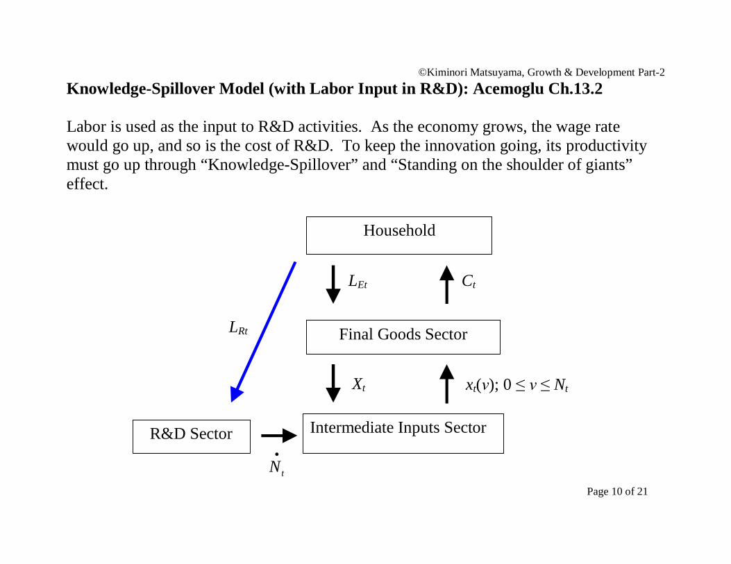
Knowledge-Spillover Model (with Labor Input in R&D): Acemoglu Ch.13.2 Labor is used as the input to R&D activities. As the economy grows, the wage rate would go up, and so is the cost of R&D. To keep the innovation going, its productivity must go up through “Knowledge-Spillover” and “Standing on the shoulder of giants” effect.

tN

Household

Final Goods Sector


LEt Ct

LRt

Xt xt(ν); 0 ≤ ν ≤ Nt


of 21

Final Good Sector: E

tNLdtxtY

)(

0

1),(1

1)(

Intermediate Input Sector: Monopoly Pricing: 1),()1)(,( tptp xx for all ν and t.

)(),( tLtx E and )(),( tLt E for all ν and t.

)()(1

1)( tLtNtY E ; )()()1()( tLtNtX E ; )(

1)( tNtw

.

R&D Sector (Innovation): “Blue prints” are now produced with the linear technology;

)()()()()( tLtNtLttN RR

. In order to keep innovation going, the R&D productivity, )(t , must grow at the same rate with the cost of R&D, the wage rate. Hence, the inclusion of the “Knowledge spillover” term. Dependence of )(t on )(tN is external to each innovator.


of 21

Labor Market Equilibrium: LtLtL RE )()( ))(( tLLLNN

ER

.

Suppose )(tN

> 0. Then, from 0)(

RR LwNVwLVN ,

)1()()()(

tNtwtV )()1()()( tL

Vttr E

.

)()1()( tLtrCC E

Aggregate Resource Constraint: XCY

EE NLCNL )1(1

1

)(1

)2()()( tL

tNtC

E


of 21

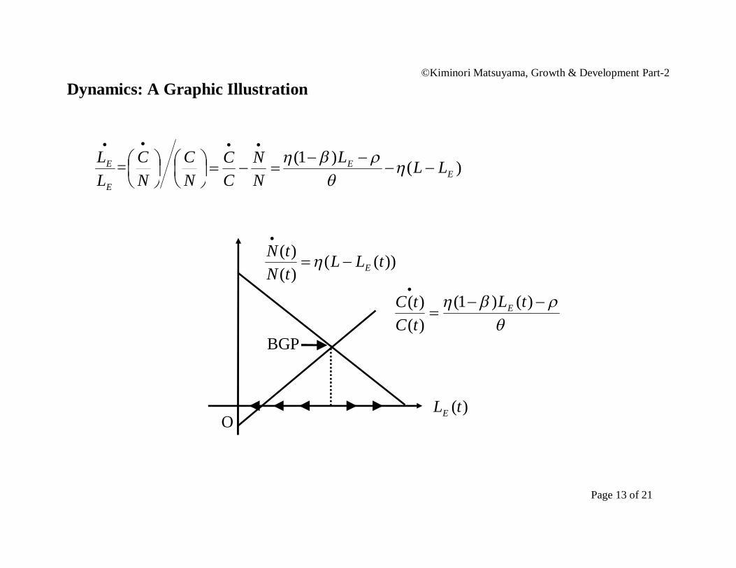
Dynamics: A Graphic Illustration

E

E

LL

=

NC

NC

NN

CC )()1(

EE LLL

O

BGP

))(()()( tLL

tNtN

E

)(tLE

)()1()()( tL

tCtC E


of 21


NN

CC

RL

1)1(* Lg .

Again, *g , as L (scale effect), , (taste effects), and (the efficiency effect).


of 21

Knowledge-Spillover Model without “Scale Effects”; Acemoglu (Ch13.3) In the above model, In order to sustain growth, it is not enough for the R&D productivity to increase in N.

It is essential that it increases at the same rate with N. Innovation and hence growth

will stop eventually, if RLNN

(λ < 1). In the data, however, the total amount of resources devoted to R&D appears to

increase steadiliy, and yet there is no associated increase in the growth rate, which suggests λ < 1.

The existence of balanced growth requires, among others, L is constant. If L grows over time, the economy will experience accelerating growth.

A large population implies higher interest rate and a higher growth. Some argue, incl. Acemoglu, that this is rejected by data, in cross-sections of countries.

These points motivate some to examine a knowledge spillover model, modified as follows:

R&D technology is by RLNN

(λ < 1) Labor supply grows at a constant rate; nt

t eLL 0 .


of 21

Along the BGP, a constant share of the labor is allocated to R&D. Hence,

tgntgN

ntLtN

tLtNtNg RR ))1((exp

))1(exp())0(()exp()0(

))(()(

)()(

11

,

which is constant if and only if

1ng . In per capita term, the growth rate is

1

nng

Indeed, one could show that the equilibrium is indeed characterized by BGP. Notes: The growth rate is no longer affected by , (taste parameters), and (the

efficiency). In this sense, it is no longer “endogenous.” The growth rate is also independent of L. In this sense, no scale effect on growth. However, there are two senses in which there are still scale effects. A faster growth rate of L translates into a higher growth rate. A large L leads to a higher output per capita.


of 21

Labor-for-intermediates Model: (Acemoglu; Ch.13.4) This was the first class of dynamic monopolistic competition model developed by

Judd, Romer, Grossman-Helpman, and others. This specification is closest to the static Dixit-Stiglitz model, as both the fixed cost

and the marginal cost of supplying intermediates are paid in labor. Final goods sector merely assembles

“intermediates” for the household. So, we could forget about the final goods sector, and “intermediates” could be viewed as differentiated consumer products, which the household assembles at home to produce the utility.

tN

Household

Final Goods Sector


Ct

LRt

xt(ν); 0 ≤ ν ≤ Nt lt(ν); 0 ≤ ν ≤ Nt


of 21

Final (Consumption) Good Sector: numeraire;

1)(

0

11),()()()(

tN

dtxtXtYtC

Representative Household:

0

)( dtetCuU t

0

)(log dtetC t

)(trCC

Note: “log” makes the marginal utility of each variety independent of other varieties. Intermediate Input Sector: Monopoly Pricing: )(),()()/11)(,( twtptwtp xx for all ν.

)(),( txtx & /)()(),( twtxt for all ν.

)()()()()()()( 11

1 txtNtNtxtNtXtC

.

From 1)()(),()( 111

1)(

0

1

twtNdztptP

tN

, 1

1

)()( tNtw .


of 21

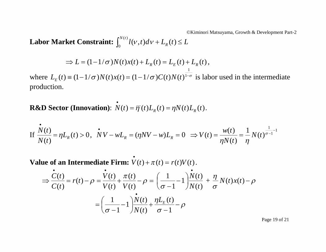
Labor Market Constraint: LtLdtl R

tN )(),(

)(

0

)()()()()()/11( tLtLtLtxtNL RER ,

where )()()/11()( txtNtLE 11

)()()/11( tNtC is labor used in the intermediate production.

R&D Sector (Innovation): )()()()()( tLtNtLttN RR

.

If 0)()()(

tLtNtN

R , 0)(

RR LwNVwLVN 1

11

)(1)(

)()(

tN

tNtwtV

Value of an Intermediate Firm: )()()()( tVtrttV

.

)()(

)()()(

)()(

tVt

tVtVtr

tCtC

)()(1

11

tNtN

+

)()( txtN

1)(

)()(1

11 tL

tNtN E


of 21

)()(

)()(

tCtC

tLtL

E

E

)()(

1)(

)()(

11

tNtNtL

tNtN E

=

))((1)( tLLtL

EE

LtLE )(

1.


0EL

11LLLL ER

11Lg N &

11

1Lgg N

c .

Again, NC gg)1( , as L (scale effect), (taste effect), (the efficiency effect). No transition path.


of 21

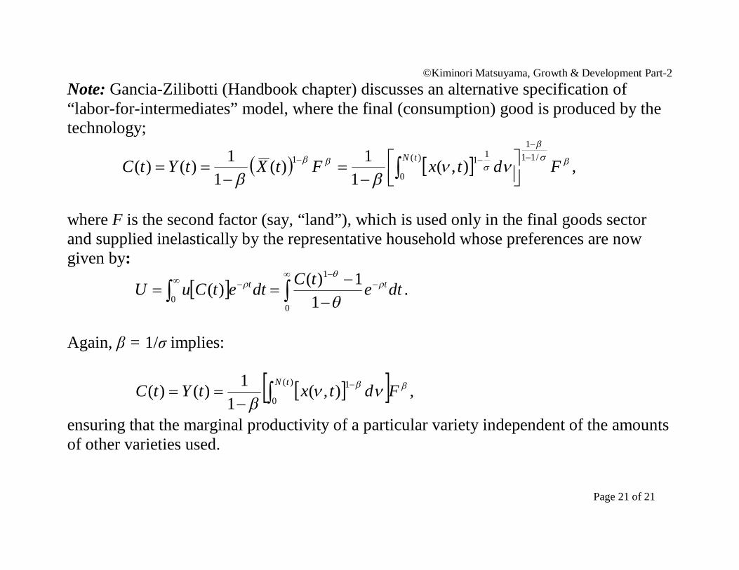
Note: Gancia-Zilibotti (Handbook chapter) discusses an alternative specification of “labor-for-intermediates” model, where the final (consumption) good is produced by the technology;

FdtxFtXtYtC

tN /111

)(

0

111 ),(1

1)(1

1)()(

,

where F is the second factor (say, “land”), which is used only in the final goods sector and supplied inelastically by the representative household whose preferences are now given by:

0

)( dtetCuU t

0

1

11)( dtetC t

.

Again, β = 1/σ implies:

FdtxtYtCtN

)(

0

1),(1

1)()( ,

ensuring that the marginal productivity of a particular variety independent of the amounts of other varieties used.

economic growth & development: part 2 horizontal

Documents