economic impact of mitigation measures
TRANSCRIPT
ECONOMIC IMPACTOF MITIGATION MEASURES
PROCEEDINGS OF IPCC EXPERT MEETING ON ECONOMIC IMPACT OF MITIGATION MEASURES
The Hague, The Netherlands, 27-28 May, 1999
Edited by: Jiahua Pan, Nico van Leeuwen, Hans Timmer and Rob Swart
INTERGOVERNMENTAL PANEL ON CLIMATE CHANGEWorking Group III: Mitigation of Climate ChangeW M O U N E P

This meeting was hosted by CPB, Netherlands Bureau for Economic Policy Analysis, in cooperationwith Intergovernmental Panel on Climate Change and Energy Modelling Forum
Programme Committee: Terry Barker, Jean-Charles Hourcade, Priyadarsi Shukla, Rob Swart, Hans Timmer, John Weyant.
Local Organizing Committee: Johannes Bollen ,Casper van Ewijk, Arjen Gielen, Jiahua Pan,Nico van Leeuwen, Rob Swart, Hans Timmer
Supporting material prepared for consideration by the
Intergovernmental Panel on Climate Change. This supporting
material has not been subject to formal IPCC review
processes.
Published by: CPB, The Hague; RIVM, Bilthoven, The Netherlands, 1999
ISBN: 90 5833 027 3 RIVM Publication No: 482550001
Cover and Lay-out: Martin Middelburg (RIVM)
CPB Contact Information:Netherlands Bureau for Economic Policy AnalysisVan Stolkweg 14 , 2585 JR THE HAGUEThe NetherlandsEmail: [email protected]://www.cpb.nl
IPCC WG III Contact Information:Technical Support UnitIPCC Working Group IIIRIVMEmail: [email protected]://www.rivm.nl/env/int/ipcc/
onderzoek in dienstvan mens en milieu

Preface
One key element of the IPCC Third Assessment Report (TAR) on mitigation of climate change is toevaluate the economic impact of policies and measures taken by industrialised countries to addressclimate change. The IPCC Expert Meeting on Economic Impact of Mitigation Measures andPolicies, organised by IPCC Working Group III and hosted by the Netherlands Bureau for EconomicPolicy Analysis (CPB) in collaboration with the Energy Modelling Forum, was intended to focuson the consequences of abatement policies in industrialised countries. Among the major objectiveswere examination of the current findings and issues arising from recent economic research in thearea, both in the context of the Kyoto Protocol and in the context of possible future agreementsbeyond Kyoto, identification of key areas of uncertainties, and generation of input for assessmentin IPCC’s Third Assessment Report on Mitigation.
With the generous co-sponsorship from the Dutch Ministry of Economic Affairs and the DutchMinistry for Housing, Spatial Planningand the Environment, the meeting took place in The Hague,27-28 May 1999. A broad set of experts from both developed and developing countries, and frominternational organisations such as the International Energy Agency and the UNFCCC, participatedin the discussion. The findings from the meeting are preliminary and highly uncertain but they canbe of value for a better understanding of the possible direction and overall trend of such impacts.These proceedings consist of a summary report, the full papers and the contribution by discussants.Although most abstracts of papers were reviewed by the Programme Committee before acceptance,no arrangement has been made for a thorough review of the full papers as included in this volume.
The activity was held pursuant to a decision of the Working Group III of the IPCC, but such decisiondoes not imply the Working Group or Panel endorsement or approval of the proceedings or anyrecommendations or conclusions contained therein. In particular, it should be noted that the viewsexpressed in this volume are those of the authors and not those of the IPCC Working Group III orthose of other sponsors.
Bert Metz Ogunlade Davidson
Co-Chairs IPCC Working Group III
3
Preface

4

Contents
Preface . . . . . . . . . . . . . . . . . . . . . . . . . . . . . . . . . . . . . . . . . . . . . . . . . . . . . . . . . . . . . . . . . . . . . . . . . . . . . . . . . . . . . . . . . . . . . . . . . . . . . . . . . . . . . . . . . . . . . . . . . . . . . . . . . . . . . . . . . . . . . . . . . . . . . . .3Bert Metz and Ogunlade Davidson
Part I Summarry Report
Summary Report . . . . . . . . . . . . . . . . . . . . . . . . . . . . . . . . . . . . . . . . . . . . . . . . . . . . . . . . . . . . . . . . . . . . . . . . . . . . . . . . . . . . . . . . . . . . . . . . . . . . . . . . . . . . . . . . . . . . . . . . . . . . . . . . . . . . . .9Jiahua Pan
Part II Issues of the Economic Consequences of Kyoto
Opening Address . . . . . . . . . . . . . . . . . . . . . . . . . . . . . . . . . . . . . . . . . . . . . . . . . . . . . . . . . . . . . . . . . . . . . . . . . . . . . . . . . . . . . . . . . . . . . . . . . . . . . . . . . . . . . . . . . . . . . . . . . . . . . . . . . . . .25Annemarie Jorritsma
Effects of Restrictions on International Permit Trading: the MS-MRT Model . . . . . . . . . . . . . . . . . . . . . . . . . . . . . . . .27Paul M. Bernstein, W. David Montgomery, Thomas Rutherford, and Gui-Fang Yang
Discussion . . . . . . . . . . . . . . . . . . . . . . . . . . . . . . . . . . . . . . . . . . . . . . . . . . . . . . . . . . . . . . . . . . . . . . . . . . . . . . . . . . . . . . . . . . . . . . . . . . . . . . . . . . . . . . . . . . . . . . . . . . . . . . . . . . . . . . . . . . . . . .57Snorre Kverndokk
Emissions Trading, Capital Flows and the Kyoto Protocol . . . . . . . . . . . . . . . . . . . . . . . . . . . . . . . . . . . . . . . . . . . . . . . . . . . . . . . . . . . . . .61Warwick J. McKibbin, Martin T. Ross, Robert Shackleton and Peter J. Wilcoxen
Discussion . . . . . . . . . . . . . . . . . . . . . . . . . . . . . . . . . . . . . . . . . . . . . . . . . . . . . . . . . . . . . . . . . . . . . . . . . . . . . . . . . . . . . . . . . . . . . . . . . . . . . . . . . . . . . . . . . . . . . . . . . . . . . . . . . . . . . . . . . . . . . .91Ben Geurts
Kyoto and Carbon Leakage: Simulations with WorldScan . . . . . . . . . . . . . . . . . . . . . . . . . . . . . . . . . . . . . . . . . . . . . . . . . . . . . . . . . . . . . . . .93Johannes Bollen, Ton Manders and Hans Timmer
Clean Development Mechanism: Discussion . . . . . . . . . . . . . . . . . . . . . . . . . . . . . . . . . . . . . . . . . . . . . . . . . . . . . . . . . . . . . . . . . . . . . . . . . . . . . . . . . . .117Robert A. McDougall
Discussion on the CDM . . . . . . . . . . . . . . . . . . . . . . . . . . . . . . . . . . . . . . . . . . . . . . . . . . . . . . . . . . . . . . . . . . . . . . . . . . . . . . . . . . . . . . . . . . . . . . . . . . . . . . . . . . . . . . . . . . . . . .121Terry Barker
5
Contents
Part III Beyond Kyoto
Developing Economies, Capital Shortages and Transnational Corporations . . . . . . . . . . . . . . . . . . . . . . . . . . . . . . . . .125Leena Srivastava and Pradeep Dadhich
Future Agreements . . . . . . . . . . . . . . . . . . . . . . . . . . . . . . . . . . . . . . . . . . . . . . . . . . . . . . . . . . . . . . . . . . . . . . . . . . . . . . . . . . . . . . . . . . . . . . . . . . . . . . . . . . . . . . . . . . . . . . . . . . . . . .135James Edmonds
Developing Country Effects of Kyoto-type Emissions Restrictions . . . . . . . . . . . . . . . . . . . . . . . . . . . . . . . . . . . . . . . . . . . . . . .153Mustafa Babiker and Henry D. Jacoby
The IPCC-SRES Stabilisation Scenarios . . . . . . . . . . . . . . . . . . . . . . . . . . . . . . . . . . . . . . . . . . . . . . . . . . . . . . . . . . . . . . . . . . . . . . . . . . . . . . . . . . . . . . . . . . .169Johannes Bollen, Ton Manders and Hans Timmer
Discussion . . . . . . . . . . . . . . . . . . . . . . . . . . . . . . . . . . . . . . . . . . . . . . . . . . . . . . . . . . . . . . . . . . . . . . . . . . . . . . . . . . . . . . . . . . . . . . . . . . . . . . . . . . . . . . . . . . . . . . . . . . . . . . . . . . . . . . . . . . . .181Steve J. Lennon
Analysis of Advantages and Disadvantages of Implementation of AIJ for China . . . . . . . . . . . . . . . . . . . . . . . . .183Ruqiu Ye, Yunhui Jin and Xue Liu
Discussion . . . . . . . . . . . . . . . . . . . . . . . . . . . . . . . . . . . . . . . . . . . . . . . . . . . . . . . . . . . . . . . . . . . . . . . . . . . . . . . . . . . . . . . . . . . . . . . . . . . . . . . . . . . . . . . . . . . . . . . . . . . . . . . . . . . . . . . . . . . .199ZhongXiang Zhang
The Kyoto Protocol: A Cost-Effective Strategy for Meeting Environmental Objectives? . . . . . . . . . . .215Alan S. Manne and Richard G. Richels
Discussion . . . . . . . . . . . . . . . . . . . . . . . . . . . . . . . . . . . . . . . . . . . . . . . . . . . . . . . . . . . . . . . . . . . . . . . . . . . . . . . . . . . . . . . . . . . . . . . . . . . . . . . . . . . . . . . . . . . . . . . . . . . . . . . . . . . . . . . . . . . .233ZhongXiang Zhang
Wrap-up Session . . . . . . . . . . . . . . . . . . . . . . . . . . . . . . . . . . . . . . . . . . . . . . . . . . . . . . . . . . . . . . . . . . . . . . . . . . . . . . . . . . . . . . . . . . . . . . . . . . . . . . . . . . . . . . . . . . . . . . . . . . . . . . . . . .239Hans Timmer
Part IV Appendix
A Meeting Programme . . . . . . . . . . . . . . . . . . . . . . . . . . . . . . . . . . . . . . . . . . . . . . . . . . . . . . . . . . . . . . . . . . . . . . . . . . . . . . . . . . . . . . . . . . . . . . . . . . . . . . . . . . . . . . . . .243
B List of Participants . . . . . . . . . . . . . . . . . . . . . . . . . . . . . . . . . . . . . . . . . . . . . . . . . . . . . . . . . . . . . . . . . . . . . . . . . . . . . . . . . . . . . . . . . . . . . . . . . . . . . . . . . . . . . . . . . . .245
6
Contents
Part I
Summary Report

8
Summary Report
Jiahua Pan1
Goal and Background
With the Kyoto Protocol entering into force, Annex B countries are obliged to comply withquantitative limitations of GHG emissions. In the agreement, “flexible” instruments are suggestedto help achieving these limitations. As the first budget period of the Kyoto Protocol is only up to2012, there is also a need to consider the architecture of the future agreements. In both the short-and long-run cases, the policies and measures in developed countries will have economicconsequences upon both the developed and the developing economies. One key element of theIPCC Third Assessment Report (TAR) on mitigation is to evaluate the likely economic impacts ofpolicies and measures taken by industrialised countries to meet their Kyoto target. There have beena few research programs on these issues and a discussion on the findings from these projects can beof great help to better understanding of the problems. Also, the direction and key issues for futureresearch on these areas need to be identified. It is against the above background that the IPCCExpert Meeting on Economic Impact of Measures and Policies taken by Annex B countries wasorganised by IPCC Working Group III and hosted by the Netherlands Bureau for Economic PolicyAnalysis (CPB) in collaboration with the Energy Modelling Forum, with financial support from theDutch Ministry of Economic Affairs and the Dutch Ministry for Housing, Regional Developmentand the Environment.
The objectives for the meeting were set to:
• Present the findings and issues arising from recent economic research in the area;• Discuss the possible architecture of future agreements beyond Kyoto;• Identify key issues for future research; and• Provide input into IPCC’s Third Assessment Report on Mitigation.
The meeting took place in The Hague, 27-28 May 1999. On the first day the economic impact ofpolicies agreed upon or discussed at COP3 and COP4 was addressed. On the second day thediscussion was on the architecture of future agreements with a longer-term view. The meeting wasdivided into four sessions with 12 papers presented. After each paper, discussants were invited toprovide comments and suggestions on the paper, followed by overall questions and a discussion. Atthe meeting, experts from CPB and the Energy Modelling Forum were invited to provide overviewson key issues at the beginning of morning sessions on both days. A panel discussion was arrangedbefore the wrap-up session on the second day. See the meeting program in Appendix A for details.
About 45 participants were present at the meeting, coming from both developed and developingcountries, and from international organisations such as the International Energy Agency and the
9
Summary Report
1 This report was drafted by Jiahua Pan of the WG III TSU on the basis of the papers and outlines received at and after the expert meetingand the notes taken during the meeting, and reviewed by the Programme Committee.

UNFCCC. Annemarie Jorritsma, the Dutch Minister of Economic Affairs addressed the audienceduring the opening session on the first day. A full list of participants is given in Appendix B.These proceedings consist of a summary report and the full papers (including one invited but notpresented at the meeting) by speakers and review papers by discussants. Papers presented at themeeting but not submitted in writing other than in the form of an outline are not included. However,efforts have been made to cover the key points of these presentations in this summary report.
Issues of the Economic Consequences of Kyoto
IntroductionThere were two half-day sessions on 27 May, chaired by Casper van Ewijk and Richard Richelsrespectively. In the opening part of the morning session, Minister Jorritsma delivered a welcomespeech in her capacity as the Netherlands Minister of Economic Affairs. She emphasised thatclimate change is an area where the policy areas of environment, energy and economics are closelyintertwined. She suggested that the focus of the climate change assessment be placed on both thefirst budget period of the Kyoto Protocol called the short run as it refers to the years up to 2012 andthe architecture of future agreements referred to as the long run. In her opinion, both the quantitativecommitments and the flexible instruments are important for the success of the Kyoto Protocol.Therefore, she suggested that compliance issues be included as an explicit part of the researchagenda on the future of climate change policy. In addition to address compliance with thequantitative commitments and active implementation of the flexible instruments both within AnnexB and globally, the Minister also considers it important to discuss possible future quantitativecommitments for non-annex B countries.
After the welcome speech by Minister Jorritsma, Hans Timmer from CPB and John Weyant of theEnergy Modelling Forum provided overviews on the issues regarding the economic consequencesand the results from earlier modelling exercises. Among the issues covered by Timmer werebaseline problems, uncertainty aspects, endogenous growth, international linkages such as trade andcapital flows, and their economic consequences on non-Annex B countries. He argued that marketfailures should be taken full account of in the overall institutional design in addition to marketmechanisms such as emission rights and taxes. The Clean Development Mechanisms as defined inthe Protocol are an example of institutional frameworks that are designed to create efficiency gainslike those that can be achieved in tradeable permit markets. This new institutional frameworksshould be excamined further because they can also lead to new coordination problems. Weyantbriefly outlined the major issues addressed by and results from 10 models2 in the literature,including AIM, CETA, FUND, G-Cubed, GRAPE, GTEM, MERGE3, MS-MRT, RICE andWorldscan developed in the United States, Europe, Australia and Japan. These macro top-downmodels conclude that, with few exceptions, there would be a loss in GDP in Annex B countries foremissions reduction without trading. With respect to the reference case, leakage is likely to resultfrom Annex B to non Annex B regions in the no trading case. The results for consumption lossesin comparison with the reference case are somewhat mixed, with net losses for OECD countries inmost cases with and without trading but with a net gain in a couple of cases for non-Annex Bcountries and the former eastern block countries. Without trading, the hot air in Eastern Europe andthe Former Soviet Union would be reduced. World oil prices appeared to fluctuate over time. Theeconomic impacts of Annex B actions on non-Annex B nations as calculated by the models aredifficult to generalise, with both positive and negative spillover effects.
10
Jiahua Pan
2 For details, please see individual papers.

Global Impacts of the Kyoto AgreementThomas Rutherford presented the results from the MS-MRT model, co-authored with researchers atCharles River Associates. The discussant for this paper was Snorre Kverndokk. In the context of aglobal agreement to limit carbon emissions, a multi-sector, multi-region trade model (MS-MRT) hasbeen developed that focuses on the international trade aspects of climate change policy, includingthe distribution of impacts on economic welfare, international trade and investment across regions,the spillover effects of carbon emission limits in Annex B countries on non-annex B countries,carbon leakage, changes in terms of trade and industry output, and the effects of internationalemissions trading.
The MS-MRT results suggest that imposing emissions limits on industrial countries with nointernational emission trading has negative impacts on the welfare of industrial and somedeveloping countries, including all the oil-producing countries, and positive welfare effects onChina and India. According to the authors’ calculations, Annex B trading moderates the impacts, andgreatly improves welfare for Russia. Global trading was calculated to be worse for China and Indiathan no trading. Russia would be considerably worse off under global than Annex B trading. Termsof trade would generally move against developing countries in favour of industrial countries whenthe former do not participate in international emission trading because the cost in industrialcountries increases, driving up the price of their exports, and their income and import demand fall,driving down the price of their imports. This is the principal reason for the negative impacts ondeveloping countries, according to Rutherford. Some developing countries can offset these terms oftrade losses because of their gains in terms of trade with OPEC and ability to shift to production ofenergy intensive goods where they have increased comparative advantage over the industrialcountries. This would also increase their gains from trade relative to OPEC. The shift of energyintensive industries of Annex B countries to non-Annex B countries when the latter do notparticipate in emission trading would be significant. As a result, carbon leakage could also besignificant in these model results, because of reduced energy efficiency and fuel substitution due tolower fuel prices in developing countries. Investment would fall in all regions, less in non-annex Bcountries and more in Annex B countries. However, the shift of industry would be moderated byAnnex B emissions trading.
These results are based on the analysis that takes into account the differences in energy intensityacross industries in different countries, and actual data on the share and energy content of importsand exports. They suggest the need to avoid competitive distortions and carbon leakage. With globaltrading, energy intensive industries could move out of developing countries, because the data showthat those countries have the least energy efficient industries and therefore are the most vulnerableto a uniform, global increase in energy costs. However, the political opposition to this de-industrialisation process is likely to be strong even if there might exist a net economic benefit fromsuch a process.
Emissions Trading, Capital Flows and the Kyoto ProtocolWarwick McKibbin presented a paper he co-authored with M. Ross, R. Shackleton and P. Wilcoxen onemission trading and capital flows under the Kyoto mechanisms. Ben Geurts of the Netherlandsprovided comments as a discussant. The theoretical appeal of an international permit program isstrongest if participating countries have very different marginal costs of abating carbon emissions – inthat situation, the potential gains from trade are largest. The results show that within Annex B andglobally, abatement costs can indeed be quite heterogeneous. These differences in abatement costs arecaused by a range of factors including different carbon intensities of energy use, different substitutionpossibilities and different baseline projections of future carbon emissions. Because of these differences,international trading offers large potential benefits to parties with relatively high mitigation costs.
11
Summary Report
The results also highlight the potentially important role of international trade and capital flows inglobal responses to the Kyoto Protocol. Regions that do not participate in permit trading systems,or that can reduce carbon emissions at relatively low cost, will benefit from significant inflows ofinternational financial capital under any Annex B policy, with or without trading. It appears that theUnited States is likely to experience capital inflows, exchange rate appreciation and decreasedexports. In contrast, the ROECD3 region as the highest cost region, will see capital outflows,exchange rate depreciation, increased exports of durables and greater GDP losses. Total flows ofcapital could accumulate to roughly half a trillion dollars over the period between 2000 and 2020.Global participation in a permit trading system would substantially offset these internationalimpacts, but is likely to require additional payments to developing countries to induce them to forgothe benefits that accrue to them if they do not participate.
The model’s results are sensitive to assumptions that determine the mitigation cost differencesamong regions. With a smaller relative control cost differential between the U.S. and other countriesin the OECD, the magnitude of capital flows to the U.S., and the costs and benefits of those flows,would all be smaller.
In the analysis, there are unavoidable uncertainties in the values of the model’s behaviouralparameters and the future values of exogenous variables. As shown by the sensitivity analysis, theresults should be interpreted as point estimates in a range of possible outcomes. It is clear, however,that in an increasingly interconnected world in which international financial flows play a crucialrole, the impact of greenhouse abatement policy cannot be determined without paying attention tothe impact of these policies on the return to capital in different economies. Focusing only ondomestic effects would miss a crucial part of the economy’s response to climate change policy. Tounderstand the full adjustment process to international greenhouse abatement policy it is essentialto model international capital flows explicitly.
AIM-based Analysis of the Economic Consequences of Kyoto – Energy Exporters vs.ImportersThe UNFCCC stipulates in Article 4 that the Parties should consider the specific needs and concernsof developing countries arising from the adverse effects of climate change and/or the impact ofmitigation measures. Such a requirement is further reiterated in the Kyoto Protocol in its Articles 2and 3. As the energy sector is likely to be most seriously affected by compliance with the Kyotomechanism, a better understanding of the possible impacts on energy importers and exporters wouldbe of great relevance to the successful implementation of the necessary policy measures. TsuneyukiMorita from the Japanese National Institute for Environmental Studies reported the modellingresults on such possible impacts. Jan Willem Velthuijsen acted as the discussant for this paper.
The key findings from the modelling exercise show that the reduction of carbon is projected to incura net cost to Annex B countries. The marginal cost per ton of carbon for Japan was calculated ashigh as $234 while that for the United States was $153, with the EU in between ($198). As a result,the projection indicates that the price of crude oil would be lower under Kyoto than the business-as-usual scenario. The price could be slightly increased if trading among Annex B countries and/orat global scale would be allowed. However, the price under trading could still be lower than thebusiness-as-usual case. One direct consequence of the price change would suggest that the Kyotoaccord would reduce global energy trade once it is implemented.
12
Jiahua Pan
3 Rest of the OECD countries.

The possible impact resulting from the reduction in oil trade may not be evenly distributed. Oilexporters, especially Middle East countries, would reduce their GDP and consumption level. On theother hand, part of energy importers including the dynamic Asian countries would benefit from theKyoto mechanisms. As to the question of how to mitigate the impacts, the model results show thatemission trading among Annex B countries would slightly increase the demand for energy andthereby a higher price of crude oil would help reduce the possible adverse impact on oil exporters.Other possible mechanisms suggested in the presentation include the role of Clean DevelopmentMechanism and compensation schemes. However, the discussion did not go into details on howthese approaches would work under the Kyoto Protocol.
Kyoto and Carbon LeakageThe issue of carbon leakage was investigated using the simulation model Worldscan, a dynamicapplied general equilibrium model, developed at CPB and discussed in a paper co-authored byJohannes Bollen, Ton Manders and Hans Timmer. The results were presented by Ton Manders at themeeting and discussed by Jean-Marc Burniaux from France. Two scenarios, A1 and B1, weretentatively used as “business as usual” or the baseline scenarios. These scenarios have beendeveloped as part of a set for consideration by the IPCC for its Special Report on EmissionsScenarios4. Both scenarios assume high growth rates, especially in non-Annex B countries. Themain difference is that in B1 very rapid autonomous improvements in energy efficiency areassumed. That makes the necessary reductions to comply with the Kyoto Protocol smaller and itgenerates a substantial amount of hot air in the former Soviet Union, even in 2020. The twoscenarios turn out to generate similar leakage rates to non-Annex B regions. However, a largedifference in leakage within the Annex B region was calculated. In 2020, reduction in Annex Bcountries would still be partly offset by induced increases of emissions in the Former Soviet Unionin the model. Typical values for the leakage rate to non-Annex B turn out to be around 20 %.Leakage in case of free emission trade could be lower compared to the case with unilateralmitigation policies.
In the analysis, the leakage was split in three different ways. First, the well-known Kaya identitywas used in which a change in emissions is disentangled into a change in production, a change inenergy intensity of production and a change in the carbon intensity of energy. The calculationssuggest that changes in energy intensity of production are more important for the amount of carbonleakage than changes in carbon intensity of energy. The latter is more important in countries thatreduce their emission than in countries that increase their emissions. Changes in the level of totalproduction are negligible as cause of leakage. Then the emissions were decomposed into emissionsthat are used for net exports of goods and services. To this end, the implicit carbon content wascomputed for all sectors, taking into account all intermediate deliveries and all imports. Most of theleakage was implicitly used for final demand in Annex B countries. That means that leakage, or theincrease in emissions in non-Annex B countries, is mainly due to more energy intensive exports toAnnex B countries and less energy intensive imports from Annex B countries.
In a sensitivity analysis, changes in emissions were split into changes that result from shifts oversectors and changes that result from shifts in production technologies. Crucial for the process aretrade elasticities and production substitution elasticities. Higher trade elasticities tend to lead tohigher leakage as a result of shifts over sectors, but slightly smaller leakage through changes in inputstructures of production. Lower substitution elasticities in the production process tend to decrease
13
Summary Report
4 These scenarios are preliminary, have not been approved by IPCC at the time when the presentation was made and are subject tochange.

leakage through changes in the input structures, but increase leakage significantly as a result ofshifts over sectors.
Clean Development MechanismThere were two presentations on this important issue: Thomas Heller from Stanford University andPriyadasi Shukla from the Indian Institute of Management, representing views from developed anddeveloping country perspectives respectively. These two presentations5 were discussed by twodiscussants, Robert McDougall and Terry Barker, with substantive comments.
The presentation by Heller examined the institutional aspects of the mechanism. For effective andefficient GHG reductions, proposals for and experiments with co-operative efforts have evolvedfrom joint implementation (JI) to activities implemented jointly (AIJ) and the clean developmentmechanism (CDM). The discussion about the CDM itself has also been evolving from complianceto a more flexible trading regime. However, there exist many issues to be negotiated, including thescope of the mechanism (sequestration), capping vs. unlimited use, hot air in Article 17 vs.additionality in Articles 12 and 6, the allocation of credits, market allocations, overall equity andequity in the CDM, multilateral mechanism vs. framework rules, private surveillance vs.administrative monitoring, the place of CDM in the long run design of a mitigation regime andratification issues.
In the institutional design of the CDM, problems are associated with adverse selection(sequestration and conservation), moral hazard (dynamic baselines), leakage issue, and that ofwasting assets and the management of a scarce pool of mitigation opportunities. The commercialviability of CDM will depend on the potential of energy efficiency, technological improvement,institutional reform, and the management of financial risks. In addition, administrative feasibility isan important element for its success. Based on the past experience in JI and AIJ activities,institutional constraints, especially those in developing countries, will have to be removed or at leastrelaxed for an effective institutional environment for CDM implementation.
The concerns over institutional issues were further emphasised in the comments provided byMcDougall. In fact he believed that too high a hope had been placed on the CDM by some of itsproponents. Rather it is argued that the CDM is likely to play only a modest role in both climatechange and sustainable development action. In his estimation, the CDM is likely to provecontentious, because it is essentially a proposal for acting “out of natural sequence” and because thesystem is to come into operation too soon for the rules to be well defined. Most fundamentally, theCDM is the product of two different agendas, the sustainable development agenda of the developingcountries, and a cost minimisation agenda by some industrialised countries. The harmonisation ofthese two agendas seems rather difficult, since large gaps remain in the two sides’ views on the roleof the industrialised countries in supporting sustainable development. Participants in the CDM maybe disappointed because the incentive to participate in the CDM is weak. On the contrary, effectivesafeguards to ensure additionality may impose burdensome delays and costs on would-beparticipants. Unlike other mechanisms, CDM projects are to be taxed to meet administrativeexpenses and to fund unrelated adaptation projects. If CDM activity will be modest, its effectivenessin promoting development in the Third World will also be modest.
The above critical view is further shared by Shukla from the perspective of the specific need ofdeveloping countries. The CDM is likely to contribute to cost-effectiveness of GHG reductions in
14
Jiahua Pan
5 No written paper has been submitted.
developed countries due to the wide differences in marginal abatement costs among countries, butthe actual benefits envisaged for developing countries seem to be rather limited. On the contrary,low global CDM supply might be beneficial to a developing country like India. If there is no CDM,the oil price is likely to be low. This means to India three possible outcomes: net GDP gain, savingsin foreign exchange, and enhancement of competitiveness. Domestic action in Annex B countriesmay also bring about favourable spillover effects to India as a result of improvement in mitigationtechnologies and reductions of future mitigation cost. Distributional issues constitute furtherconcerns for developing countries. In case of India, the gains and losses under different permitschemes could account for several percentage points of its GDP and it is emphasised that the stakesfor India could be “high”. The conclusion was drawn from his presentation that fairness must beensured for the CDM, which requires burden sharing, fair competition, minimisation of welfarelosses and the adoption of a precautionary principle.
Together with other participants, Barker joined the interesting debate as a discussant to Shukla’spresentation. Three sets of comments were added to the debate on the effects of the CDM as aflexible instrument on the Kyoto Protocol. The first issue is concerned with uncertainty of the sizeand scale of incremental abatement costs. There will be huge differences in costs depending on thetechnologies involved, the information available, the incomes of those making the mitigationdecisions, and the time available for the schemes to be planned and to operate. The usual assumptionon lower incremental costs in developing countries can be questionable. The second point concernsmacroeconomic and environmental effects. Learning-by-doing and economics of specialisation andscale may well mean that the net benefits increase or the costs decrease. On the other hand if therevenues from the use of fiscal instruments e.g. carbon taxes are used to reduce one distortionarytax after another, starting with the most distortionary, then as the taxes are removed, the net benefitsshould decrease. Environmental effects of CDM schemes such as reductions in other emissions anddamages associated with the reduction in GHG emissions should also be taken into account in thecalculation of the social net benefits of CDM schemes.
The third point touched upon relates to additionality: how can participants be assured that theoutcomes of a CDM scheme will indeed be additional to those which would otherwise haveoccurred? In the case of a CDM project there are two sides to the additionality problem: i) how canthe non-Annex B country be assured that the CDM funding will not replace other financialassistance? And ii) how can the Annex B country be assured that the mitigation will be additional?The problems here can be alleviated by two requirements. One is that a proportion of the fundingfor the CDM scheme (say 50%) should be available to the receiving country for discretionary use.And the other suggests that Only 50% of the GHG savings be available to the Annex B country asa contribution to its Kyoto mitigation requirements.
Beyond Kyoto
IntroductionThe sessions on Beyond Kyoto were chaired by Mohan Munasinghe of Sri Lanka and Bert Metz ofthe Netherlands. A longer-term view is necessary as the Kyoto commitments are set up to the period2008-2012 only. In addition to six presentations, an overview on the EMF – 17 model comparisonwas presented and panel discussion conducted.
John Weyant briefly reviewed the results of the Energy Modelling Forum models, discussed thepost-Kyoto frontiers and suggested directions for future research. The challenges ahead would
15
Summary Report
include three issues. One is the flexibility issue: where, when, how and why flexibility. The howquestion would involve research and development, technology transfer, information programs, sinksetc. More comprehensive approaches are indicated. Second, the issue of sustainability, equity anddevelopment attracts lively debates in both the academic and the policy circles. The solutions tothese issues are complicated by the differences in views and in many cases conflict amongeconomic, ethical, social, political and ecological principles. Incentive compatibility constitutes thethird key issue. Coalitions are likely to be formed and linkages to other global issues must beestablished. Three areas of future directions are suggested, notably the basic models, internationaltrade and technological issues.
Developing Economies, Capital Shortages and Transnational Corporations (TNCs)Transnational companies may have a major role to play within and beyond Kyoto. A majority oftransnational corporations are based and controlled in industrialised countries. They are equippedwith advanced technologies, capital resources, and managerial skills. There is an incentive for themto invest in developing countries for higher returns. In developing countries, there is usually ashortage of capital and lack of appropriate technology. Through direct foreign investment indeveloping countries, ancillary benefits are likely to be accrued, including additional supply ofscarce capitals, transfer of technology and management know-hows, promotion of trade andexports, and generation of employment opportunities and training of skilled workers. All thesewould contribute to GHG reduction in developing countries in the long run. However, LeenaSrivastava argued in her presentation that negative effects also exist because of conflicts of interest.The rising power of the transnational companies is also considered a cause of concern as theydominate the production and trade at global level. Considering the positive impact of TNCs onGHG reductions, they should be treated more explicitly in future agreements on climate change.However, issues regarding the role, position and entitlement of TNCs should be further investigatedin the design of emission trading regimes. The views were partly shared by Thomas Heller, thediscussant for the presentation, although more emphasis was on institutional constraints in thediscussion.
Future AgreementsJames Edmonds discussed principles upon which future agreements to mitigate greenhouse gasemissions might be framed. The current foundation for international action is the FrameworkConvention on Climate Change (FCCC), whose ultimate objective is: the stabilisation ofconcentrations of greenhouse gases at levels, which would prevent dangerous anthropogenicinterference with climate systems. Neither the FCCC nor the 1997 Kyoto Protocol containsprovisions sufficient to achieve this objective. Further agreements will be needed. Theseagreements must confront three broad challenges: extension of the reference time frame to acentury;control of costs; and expansion of the list of nations with quantifiable emissions limitations.
Several research findings are relevant. First, stabilisation of CO2 concentration implies that netglobal emissions may grow for a time, but must eventually peak sometime in the next century andthen decline thereafter. But, economic theory suggests that global cost minimisation requires thateveryone value a tonne of carbon equally, and that the common value initially be small but rise atthe rate of interest plus the rate of removal of carbon from the atmosphere. This allows for theorderly turnover of capital stock, time to conduct R&D, prevents lock-in to early versions of newtechnologies, which are rapidly improving, and provides time for infrastructure development.Achieving these conditions requires the development of mechanism, which are consistent withprinciples of fairness and equity, by which non-Annex B nations can participate. Two exampleswere discussed. Expanded programs to develop and deploy technologies including conservation,
16
Jiahua Pan

non-carbon emitting energy forms, and mechanisms for the capture and sequestration of carbon arealso needed.
The logic and comprehensiveness of the architecture proposed by Edmonds was highly appreciatedby Thomas Rutherford as discussant, with further suggestions to improve the framework.
Developing Country Effects of Kyoto Emissions RestrictionsThe paper by Mustafa Babiker and Henry Jacoby on developing country effects was presented byMustafa Babiker and discussed by Mohan Munasinghe. The magnitudes of the long-term economicimpacts are highly uncertain, but the analysis gives an idea of what these impacts might be, as wellas how they are transmitted through the international trade system. The greatest loss would beimposed on energy exporters, and the more dependent a country is on these exports the greater thepercentage effect on its economic welfare. So a country like Mexico, with a large and diversifiedeconomy would be much less influenced than the nations of the Persian Gulf (RME), for whom oilrevenues constitute a large faction of GNP. The elasticities of demand by importing countries, andof supply by the non-OPEC exporters, combine to produce a market condition where efforts to resistthe fall in oil price resulting from Kyoto restrictions could lead to still lower overall OPEC revenue.Attempts to do the same by a smaller group within OPEC would lead to even worse results for thosetaking action to support the price. The distribution of burdens differs depending on the treatment ofexisting fuels taxes in the enacting of carbon policies; and the presence or absence of emissionstrading is even more significant. In general, those importing energy would benefit from morestringent the policies, and the energy exporters would lose. Moreover, emissions trading and taxharmonisation would look different depending on a nation’s position on this scale. The intensity ofthe response will be approximately in proportion to the weight of the energy sector in the nationaleconomy.
Economic Analysis of the IPCC – SRES Stabilisation Scenarios Using WorldscanThe newly produced IPCC emission scenarios6 were preliminarily used as the basis for a simulationanalysis using the Worldscam model developed in the CPB. The work was undertaken by JohannesBollen, Tom Manders and Hans Timmer of the CPB and presented at the meeting by JohannesBollen.
There were three policy cases in the simulation exercise: early versus delayed response; the KyotoProtocol with Annex B trading; and global trading after the first Kyoto budget period. Two sets ofconclusions were drawn from the study. Within the “A1” scenario, it appears from the modellingresults that (1) 550 ppmv could be achieved at moderate costs; (2) delayed response may havenegative economic consequences for non-Annex B countries; (3) early response may have negativeeconomic consequences for Annex B countries; (4) the income effects could be reversed throughpermit allocation schemes; (6) a delayed response seems globally beneficial from an economicperspective; and (7) the price distortion in the end may be large. The second set of conclusionssuggest that delaying the global response is likely to be beneficial at global level because it presentsovershooting in the medium run and free-riding behaviour due to discounting future cost/benefits.However, due to income transfers from permit trade, conflict of interests may occur.
The comments by Steve Lennon from South Africa and other experts question some of theconclusions while acknowledging the vigorousness of the modelling method. Some of the key
17
Summary Report
6 These scenarios were developed in the IPCC Special Report on Emissions Scenarios and not yet approved by the Panel at the timeof the meeting.

features are still to be fully incorporated. Examples include technological progress during the periodfor over one-century, leakage of GHGs, the learning-by-doing losses under delayed response, andancillary benefits. In the proposed IPCC SRES scenarios, A1 is characterised with rapid growth,technologically optimistic, major reductions in per capita income. If other scenarios were used, theconclusions could be very different.
The Kyoto Protocol: A Cost-Effective Strategy for Meeting Environmental Objectives?For many Annex B countries, the cost involved in compliance with the Kyoto Protocol is a majorsource of concern. The presentation by Richard Richels was helpful for improving theunderstanding of compliance costs. Three questions were examined in the study by Alan Manne andRichard Richels: What are the near-term costs of implementation? How significant are the so-called“flexibility provisions”? And, is the Protocol cost-effective in the context of the long-term goals ofthe Framework Convention? This analysis was based on MERGE (a model for evaluating theregional and global effects of greenhouse gas reduction policies), an intertemporal marketequilibrium model. Three scenarios were explored using the model for answering the questions: 1)no trading, 2) Annex 1 trading plus CDM, and 3) full global trading. These three options arerepresentative of alternative implementations of the Kyoto Protocol, with the last as an upper boundon the CDM’s potential to reduce GDP losses.
In the no trading case, the value of emission rights in the United States in 2010 would approach$240 per ton. With Annex 1 trading plus CDM, the value would drop to slightly less than $100 perton. As might be expected, the value of emission rights would be lowest with full global trading.Here, it would fall below $70 per ton. In terms of the GDP losses, details were calculated for theUS. The highest losses would occur in the absence of trade, exceeding $80 billion dollars in 2010,accounting for about one percent of US GDP. To the extent that trade is introduced, losses woulddecline. In the most optimistic scenario (full global trade), losses were estimated to beapproximately $20 billion or one-quarter of one percent of GDP in 2010.
Assuming full global participation in an international market for carbon emission rights, the impactsof limits on emission rights one country could buy were analysed. The losses in 2010 would be twoand half to three times higher with the constraint on the purchase of carbon emission rights. As nospecific obligations are imposed on countries outside Annex 1, there is the possibility of “leakage”.The overall results indicate that permit trading does not seem to lead to a dramatic increase incarbon emissions outside Annex 1, suggesting that an international leakage problem could bemanageable.
With respect to the long-term stabilisation objective, there are different pathways for stabilisingconcentrations at 550ppmv (twice pre-industrial levels) by 2100, including 1) “Kyoto followed byarbitrary reductions”; 2) “Kyoto followed by least-cost”; and, 3) “least-cost”. Following a least-coststrategy suggests that a gradual transition to a less carbon-intensive economy is preferable to oneinvolving sharper near-term reductions. With the least-cost paths, the value would be relatively lowin the early years ($11 per ton of carbon in 2010), and it would rise gradually over time. With“Kyoto followed by least-cost”, the value was calculated at $130 per ton in 2010 and then wouldtrack the least-cost path thereafter. In the case labelled “Kyoto followed by arbitrary reductions”,the incremental value of emission rights would start at about $160 per ton and it would remain high.In terms of the economic impact on the global economy, “Kyoto followed by arbitrary reductions”would be the most expensive of the three paths. “Kyoto followed by least-cost” could be aconsiderable improvement, but would still be 40% more expensive than embarking on the mostcost-effective mitigation pathway from the outset.
18
Jiahua Pan
The results appear rather indicative of the policy directions, but there are several concerns over theresults presented by Richels. As commented by ZhongXiang Zhang, emphasis on global cost-effectiveness tends to underplay distributional issues. The authors also acknowledge the critics thatMERGE tends to overestimate the costs of mitigation because of the assumptions used in the model.In addition, issues regarding the power of the market, short-term macro shocks and effectiveness ofdomestic policies may need further investigation before a firm conclusion can be drawn on thepractically achievable benefit from emissions trading.
The above issues are partly explored in the paper submitted by Ruqiu Ye of China and the commentson that paper by ZhongXiang Zhang. Although the paper was not presented due to travel problemsby Ye, it is included in the proceedings.
Climate Policies Beyond Kyoto?Panel discussants presented their views on climate policies beyond Kyoto. Yvo de Boer from theNetherlands Ministry of Environment suggested that the targets for the second budget period bedifferentiated in accordance with income level, types of commitments and time of commitments. Itis also noted that the divergence of the targets in the early period should be converged at later stages.The modelling exercises have touched upon many important issues regarding economic impactsfrom policies and measures from Annex B countries, but further efforts would be required toexamine more explicitly the impacts on non-annex B countries and on the impact of 1st commitmentperiod on the 2nd budget period. In particular, de Boer points out that much of the modelling workhas been undertaken for and in developed countries and therefore more work should be planned andcarried out for and in developing countries.
Bill Hare from Green Peace stressed that concentration limits are inadequate to drive policiesdesigned to avoid dangerous climate change for the 2nd budget period, because of economic,environmental and policy uncertainties. Due to the constraints faced by developing countries, theyas a group are more vulnerable and at risk. With the materials from recent literature, Hare considersthat there exists an urgency to take policy measures to mitigate climate change. If emissions are toohigh then achievement of climate objectives much below 500 ppmv CO2 could become extremelydifficult. A number of suggestions were offered: (1) economic decision making under uncertaintyframeworks needs to be developed further and main-streamed in the IPCC assessment; (2) “short”term climate policies (e.g. next 10-15 years) need to preserve capacity for future policy makers tomeet strong climate policy goals and (3) analysis needs to be oriented at achieving both long andshort term goals simultaneously. Jonathan Pershing from the International Energy Agency points outthat there are limitations using the modelling approaches. New technologies are developed andbrought into use and the behaviour of the consumers will become more climate friendly. Carbon hasbeen valued in many current investment decisions. In designing future agreements, many factorsshould be taken into account, including participation, timing, development and environment,legislative issues, and coverage of GHGs. It is also necessary to consider the interaction betweenthe short and long term targets.
Mohammad Al Sabban and Priyadarsi Shukla participated in the panel discussion from a developingcountry perspective. Al Sabban believes that oil producing, especially OPEC, countries are likely tosuffer from any policy measures for meeting the Kyoto commitments by Annex B countries. Asindicated in many of the studies, oil price is likely to be lowered due to adoption of mitigationpolicies. He suggested that the tax system on energy should be reconsidered. Oil in the EU is heavilytaxed while on the other hand subsidies to fossil fuels especially coal prevail in many countries. Theoil exporters should be partly compensated with the reform of the current tax system. Also the issueof carbon sequestration should be further examined. Shukla made three sets of comments. The first
19
Summary Report
one states that any post-Kyoto agreement should take into account the principles of equity andsustainability. Regarding the policy alternatives, Shukla indicated that they should consider thedifferent needs, different stages of development and the specific circumstances of developingcountries. In the modelling exercise, other considerations including environmental and equity inaddition to economic goals should be incorporated. Any policies for the post Kyoto period are likelyto result in gainers and losers and the third set of comments from Shukla are concerned withdistributional problems. We should not only consider how to compensate but also consider how todistribute compensation.
Key Conclusions and Points for Further Research
At the meeting a questionnaire was distributed asking for information on the major points and issuesfrom this expert meeting. Hans Timmer on behalf of the organising committee summarised a fewkey points from the meeting and for the follow-up work.
• Methodologies: modelling approaches are very useful tools to analyse the possible outcomes fromdifferent policy choices under a given set of conditions. However, there is a lack of communicationbetween the modellers and policy makers. The component of “development” is not explicitlyincluded in the models. Therefore, there is a need to integrate the economic developmentcomponent into the climate change simulations. In addition, non CO2 GHGs and non energy CO2need to be included in the modelling exercises while acknowledging the weak knowledge baseregarding the costs of sink enhancement and of controlling of the relevant trace gases. The modelsshould be improved to take into account sequestration technologies, burden sharing and equity
• Costs of mitigation: International cooperation through trade in emission rights is likely to reducemitigation costs. The magnitude of the savings will depend on several factors. These include thenumber of countries participating in the trading market, the shape of each country’s marginalabatement cost curve, the extent to which buyers can satisfy their obligation through thepurchase of emission rights, and the impacts on the financial markets. However, model resultsshould be interpreted carefully with essential understanding of the assumptions and conditions.
• Economic impact on developing countries: The results of modelling analyses show a mixedpicture with respect to the impact on GHG-mitigation in Annex-I countries on developingcountries. Vulnerable countries include oil exporting countries. Impacts through changes incapital flows and instabilities of exchange rates can be significant.
• Emissions trading: Theoretically, global intertemporal trading is economically the most efficientsolution to limit GHG emissions and eventually stabilise GHG concentrations. Partial steps inthat direction may introduce undesirable distortions. However, because of current realities, thediscussions concluded that a rapid introduction of a global market for emissions rights isprobably more dangerous than a first incomplete move towards that ultimate goal.
• Carbon leakage: Mitigation of GHG emissions in Annex-B countries will probably lead toincreased emissions in other countries. The extend to which this may happen, according to theeconomic models used in the presentations, is very uncertain and depends on issues such as thebaseline scenario used, the level of integration of non-Annex-B countries in the world economy,and the price elasticity of energy supply.
20
Jiahua Pan

• Clean development mechanism (CDM): As an important flexibility mechanism, it may have thepotential for cost-effective compliance with the Kyoto targets. However, the realisation of suchpotential will have to depend on a well designed and functioning institutional framework andpolitical feasibility. A point of concern is that CDM, being not a general but a projects relatedmechanism, leads to unequal marginal abatement costs within developing economies. Thiswould introduce economic inefficiencies. Issues like the business-as-usual baseline, leakage andthe role of transnational companies will have to be addressed to make the mechanism workeffectively.
• Baseline issues: For modelling exercises, usually a reference scenario or baseline has to beassumed. Such a baseline depends on assumptions with respect to issues such as globalisationtrends, the international division of labour and the relative growth rates of emerging economies.It has large implications for model results. The baseline is not only an assumption in the models,but also a key issue for negotiators to be agreed upon, e.g. for the implementation criteria of theKyoto mechanisms or other possible future agreements. Some factors such as internationalleakage, institutional aspects, and change of behaviour are important for the understanding of thebaselines, especially for the long-term baselines.
• Future agreements: The time path for GHG stabilisation has important policy implications. Bothintra- and inter-generational burden sharing should be taken into account. Point of departure isthat GHG concentrations have to be stabilised according to the UNFCCC. And in order tostabilise GHG concentrations, all countries would eventually have to be part of a futureagreement. Equity considerations should primarily focus on the entry time, but more on thepermit allocation as permits are actually a tradable asset or good in the international market.From an analytical and political point of view, a rigid distinction between the Kyoto Protocol andfuture agreements is unsatisfactory.
• Treatment of ancillary benefits: Ancillary benefits may take a large share of the total benefitresulting from mitigation policies, but inadequate treatment has been given to this in themodelling exercises
21
Summary Report

22
Part II
Issues of the Economic Consequences of Kyoto

24

Opening Address
Annemarie Jorritsma, Minister of Economic Affairs
Ladies and Gentlemen,
I am pleased and honoured to have the privilege to open this Expert Meeting of theIntergovernmental Panel on Climate Change. Climate change is an area where the policy areas ofenvironment, energy and economics are closely intertwined. As Minister of Economic Affairs -responsible for both energy and economic policy - I am therefore intensively involved in climatechange policy.
This type of meeting allows for an open discussion on a very important matter. Unfortunately, asclimate policy is now a highly political issue, such open discussions are quite rare. Being aneconomics Minister, I know that anything that is rare is highly valued. I was therefore more thanwilling to invest both time and money in the organisation of this meeting. I am sure that for theEnvironment Minister Mr. Pronk, it was this high rate of return to investment that did the trick.
However, others have contributed much more than Mr. Pronk and I have done. For instance: The Stanford Energy Modeling Forum, which already commenced last night and will continue untilSaturday morning; the Technical Support Unit of Working Group III of the IPCC, which alsoparticipates in the organising committee and the Netherlands Bureau for Economic Policy Analysis,which, as Chair of the organising committee, has successfully prepared the ground for this importantmeeting. Many people from all these organisations have worked hard to ensure the success of thismeeting.
The participation of speakers and discussants from a broad range of countries is essential for thistype of meeting. I am therefore very pleased to see so many guests from across the globe, and I wishto thank you all for coming. Your contribution to the debate will be the central product of these twodays.
The purpose of this meeting is to design proposals for future research and inputs for the ThirdAssessment Report on Climate Change, to be published by the IPCC in the near future. The focuswas placed on both the first budget period of the Kyoto Protocol - called the short run, as it refersto the years up to 2012 - and the architecture of future agreements – referred to as the long run. Ifirmly believe that the longer-term perspective is of the utmost importance for our views on the shortrun. Therefore, I express my hope that today again, the long-run focus is taken as a starting point inthe discussions.
Regarding the relationship between the long run and the short run - or preferably, a not so long run- I wish to make two comments:
In my opinion, the flexible instruments are as important to the success of the Kyoto Protocol as thequantitative commitments. They are the two pillars on which the Protocol rests. By agreeing to the
25
Opening Address

quantitative commitments, the Annex I parties have acknowledged their historical responsibilitiesfor the current concentration of greenhouse gases in the atmosphere. By agreeing to the flexibleinstruments, the non-Annex I parties have shown that they, too, are serious about the global natureof the problem. I believe that we should focus on compliance with the quantitative commitmentsand on actively implementing the flexible instruments, both within Annex I and globally. This is justas important for the long run as is a serious discussion about future quantitative commitments fornon-Annex I countries. I sincerely hope that the discussions today and tomorrow will provide newinsights on these matters. Looking at the program, the speakers and the discussants, I have no doubtthat the meeting will be of a high standard.
A second point that I believe to be very important is enforcement of the protocol. As we all know,it is difficult to ensure compliance with an international treaty, even after the parties have ratified it.We need an effective compliance regime for the Kyoto protocol, with clear-cut sanctions for casesof non-compliance. I honestly do not believe that the protocol can be used to tackle climate changeeffectively in the long run if this precondition is not met. It simply lacks credibility. I know that forscientists, the compliance issue is a difficult topic to deal with. However, I wish to point out thatmany analyses start with the implicit assumption that compliance is guaranteed. I would like tosuggest that compliance matters be an explicit part of the research agenda resulting from thismeeting.
Ladies and Gentlemen, I think this meeting will be most interesting and very useful for all those concerned with theinternational issues of climate change policy. I hope that the discussions will lead to a robustresearch agenda on the future of climate change policy. I for one will be looking forward to learningthe results. For the present, I wish you much inspiration for the discussions.
Thank you.
26
Annemarie Jorritsma

Effects of Restrictions on International Permit Trading: The MS-MRT Model1
Paul M. Bernstein, W. David Montgomery, Thomas F. Rutherford, Gui-Fang Yang
Abstract
A number of proposals to restrict international emissions trading have emerged in negotiationsdealing with implementation of the Kyoto Protocol. This paper uses a Computable GeneralEquilibrium (CGE) model of international trade developed by the authors to analyze some of theseproposals. The proposed restrictions include limits on the share of a country’s obligation to reduceemissions it may satisfy through purchases of permits, restrictions on the ability of the Soviet Unionto sell permits in excess of those needed to cover its baseline emissions, other restrictions on permitsales, potential exercise of monopoly power by sellers of permits, and restriction of permit tradingwith developing countries to permits generated through the Clean Development Mechanism(CDM). Unrestricted trade among Annex I countries can reduce costs present in the case of nopermit trading by about 50 percent, and would remove some of the trade distortions created by theasymmetric obligations of Annex I and non-Annex I countries. Unrestricted global trading isnecessary to eliminate trade distortions fully and would produce another 50 percent cost reduction.
Restrictions on Annex I countries’ purchases and sales of emissions permits could eliminate half ormore of the possible gains from emissions trading. Although Russia could exercise monopolypower by restricting sales and raising permit prices, proposed limits on sales would result in evengreater output restraint and raise prices still higher. Banning sales of excess permits by Russiawould make all countries, including Russia, worse off because that limit greatly exceeds the levelof sales restrictions that a monopolist would choose. At the same time, the restriction wouldeconomically harm all purchasers. Limiting emissions purchases affects regions differently butdepresses welfare globally. If permit purchases were limited to 50 percent of a country’s emissionsreduction obligation, the U.S. might even benefit under Annex I trading at the expense of Japan andEurope, who purchase proportionately more permits than the U.S. Purchase restrictions would beparticularly damaging to the U.S., however, if trading were extended to developing countriesbecause, under unrestricted global trading, the U.S. would want to satisfy 70 percent or more of itsobligation through purchases of emissions permits. Finally, the CDM would fail to reduce much ofthe costs or competitive distortions that exist under unrestricted Annex I trading because the CDMwould not correct the disparity in energy prices applying to all industries and activities not includedin CDM projects.
27
Effects of Restrictions on International Permit Trading: The MS-MRT model
1 The authors are grateful for comments and suggestions from the participants in the EMF 16 workshops in Washington, DC, and atStanford University and Snowmass during 1998, as well as to Edward Balistreri of CRA for his contributions to developing bothconsistent measures of welfare and an approach to treatment of international trade issues. We gratefully acknowledge financial supportfrom the Business Roundtable, the Electric Power Research Institute, and the American Petroleum Institute. All statements and findingsare the sole responsibility of the authors.

Overview
The Kyoto Protocol, signed in December 1997 but not yet ratified by a number of countriesincluding the United States, defined the next steps to be taken to reduce global greenhouse gasemissions. It also left unsolved a wide range of questions about the future course of climate changepolicy. The Protocol calls for the majority of industrialized countries to limit their emissions ofgreenhouse gases by the first decade of the next century, and includes several “flexibilitymechanisms” that could significantly reduce costs for some countries. Developing countriesundertook no commitments to limit their emissions, and insisted that proposed procedures underwhich such commitments could be made be deleted from the Protocol. Flexibility mechanismsincluded coverage of six greenhouse gases, provisions for international emissions trading, creditsfor reforestation and other actions that remove greenhouse gases from the atmosphere (“sinks”), anda “Clean Development Mechanism” under which industrial countries could finance and gain creditfor emissions reductions in developing countries. Virtually all of the details concerning theflexibility mechanisms were left open for further negotiation. These include such issues as the roleof developing countries in the overall emissions reduction effort, and the scope and design of aninternational emissions trading system.
In the aftermath of the Kyoto negotiations, countries have argued extensively over the equitablestructuring of an international permit trading protocol. Unrestricted, comprehensive, and properlydesigned, an international emissions trading system would significantly reduce the global costs oflimiting greenhouse gas emissions. Nevertheless, parties to the ongoing negotiations have takenmutually incompatible positions on how emissions trading should be implemented. The UnitedStates has advocated unrestricted emissions trading, extended as rapidly as possible to include keynon-Annex I countries. The European Union and a number of developing countries have proposedtight restrictions on emissions trading, and oppose any efforts to include non-Annex I countries.Russia has made it clear that its participation in the Kyoto Protocol is contingent on its unrestrictedability to sell permits to other Annex I countries. Furthermore, all sides debate the meaning oflanguage in the Protocol that emissions trading must be “supplementary” to domestic abatementefforts.
Restrictions on emissions trading could eradicate most of such a system’s potential benefits.Curtailing Russia’s ability to sell permits or, conversely, efforts by Russia to restrict sales in orderto raise prices could have a major negative impact. Imposing a ceiling on purchases by the U.S. orother countries to enforce a restrictive notion of “supplementarity” would probably have a similareffect. Ultimately, such restrictions would lead to higher permit prices in the United States, lowerpurchases of permits on international markets, and losses in GDP and exports that wouldapproximate levels to be expected in a no-trade regime.
Currently, the outcome of the Kyoto Protocol remains highly uncertain; thus, the final form ofemissions trading is unclear. Because of the great uncertainties involved, this paper analyzes threepossible emissions trading regimes under a number of different trading restrictions. To assess thepossible impacts on world regions from this diverse set of possible outcomes, we employed ourMulti-Sector, Multi-Region Trade (MS-MRT) model. Since this model is a fully dynamic, generalequilibrium model of trade, it accounts well for the interactions among industries and regions thatresult from international policies.
In the next section, we describe the MS-MRT model, providing an overview of the model structureand key elements. We then report the results from three basic emissions trading regimes that wedenote as our core scenarios: no trading among regions in emissions permits, unrestricted trading
28
Paul M. Bernstein, W. David Montgomery, Thomas F. Rutherford, Gui-Fang Yang

among Annex I countries, and unrestricted trading among all regions. After presenting results fromthese scenarios, the paper analyzes a number of different restricted trading scenarios. First, itdescribes the modeling methodology for these scenarios, then presents results and discusses howrestrictions on trading affect the level and distribution of costs of compliance with the KyotoProtocol.
Description of the MS-MRT Model
The Multi-Sector Multi-Region Trade (MS-MRT) Model is a dynamic, multi-region generalequilibrium model that is designed to study the effects of carbon restrictions on trade and economicwelfare in different regions of the world. The model includes a disaggregated representation ofindustries, based on the GTAP4 dataset, so that differences in energy intensities across countries anddifferences in the composition of industry can be taken into account. It can represent a wide varietyof international emissions trading regimes, define trading blocs composed of any grouping ofregions, and place any set of constraints on both purchases and sales of emissions permits. Themodel computes changes in welfare (calculated as the infinite horizon equivalent variation),national income and its components, terms of trade, output, imports and exports by commodity,carbon emissions, and capital flows. It is fully dynamic, with saving and investment decisions basedon full intertemporal optimization.
Conceptually, the MS-MRT model computes a global equilibrium in which supply and demand areequated simultaneously in all markets. The model assumes full employment and there is no money.There is a representative agent in each region, and goods are indexed by region and time. The budgetconstraint in the model implies that there can be no change in any region’s net foreign indebtednessover the time horizon of the model. Even though there is no money in the model, changes in theprices of internationally traded goods produce changes in the real terms of trade between regions.All markets clear simultaneously, so that agents correctly anticipate all future changes in terms oftrade and take them into account in saving and investment decisions. The MS-MRT model iscalibrated to the benchmark year 1995, and solves in five-year intervals spanning the horizon from2000 to 2030.
In order to capture some of the short-run costs of adjustment, elasticities of substitution betweendifferent fuels and between energy and other goods vary with time. The model is benchmarked toassumed baseline rates of economic growth and a common rate of return on capital in all countries.The rate of growth in the effective labor force (population growth plus factor-augmenting technicalprogress) and the consumption discount rate are computed to be consistent both with the assumedrates of growth and return on capital, and with zero capital flows between regions on the balancedgrowth path.
In the form used for the EMF study, the MS-MRT model divides the world into ten geopoliticalregions (see Table 1).
Six industries are represented in the MS-MRT model structure:• Four energy forms: oil, coal, natural gas, and electricity; and• Two non-energy goods: Energy-Intensive Sectors (EIS), and All Other Goods (AOG).
The MS-MRT model uses an Armington structure in its representation of international trade in allgoods except crude oil, and places no constraints on capital flows. Crude oil is treated as ahomogeneous good perfectly substitutable across regions. For all other goods, we assume that
29
Effects of Restrictions on International Permit Trading: The MS-MRT model

domestically produced goods and imports from every other region are also differentiated products.Domestic goods and imports are combined into Armington aggregates, which then function asinputs into production or consumption.
The model includes the markets for the three fossil fuels. Electricity is produced using these fuels,capital, labor, and materials as inputs. Crude oil trades internationally under a single world price.Natural gas and coal are represented as Armington goods, to approximate the effects ofinfrastructure requirements and high transportation costs between some regions. Depletion isassumed to lead to rising fossil fuel prices under constant demand, but the relation betweendepletion effects on the supply of oil, gas, and coal and the actual supply of these fuels is ignored.That is, the model does not keep a record of the current stock of each fuel in each time period.World supply and demand determine the world price of fossil fuels. Current energy taxes andsubsidies are included in each country’s energy prices. The carbon-free backstop, represented as acarbon sequestration activity that requires inputs of non-energy goods, establishes an upper boundon world fossil fuel prices.
Non-Technical Discussion of the MS-MRT Model Structure
This section offers a non-technical discussion of the important elements of the MS-MRT model:production, household behavior/consumer choice, international trade, savings and investment, andcarbon restrictions. It relies largely on diagrams to illustrate the nesting structures used in theutility and production functions and the definitions of markets.2
Production of the Non-Energy GoodsThe MS-MRT model represents non-energy production in two sectors. In producing non-energygoods, the model accounts for regional differences in factor intensities, degrees of factorsubstitutability, and the price elasticities of output demand in order to trace back the structuralchange in industrial production that is induced by carbon abatement policies.
30
Paul M. Bernstein, W. David Montgomery, Thomas F. Rutherford, Gui-Fang Yang
Table 1 Regions in the MS-MRT Model
Member ofCode Region OECD Annex I
USA United States Yes YesJPN Japan Yes YesEUR Europe Union of 15 Yes YesOOE Other OECD Yes YesFSU Eastern Europe and Former Soviet Union No YesCHI China and India No NoSEA Korea, Singapore, Taiwan, Thailand, and Malaysia No NoOAS Other Asia No NoMPC Mexico and OPEC No NoROW Rest of world No No
2 For a mathematical description of the model, see Bernstein, Rutherford, and Montgomery, "Trade Impacts of Climate Policy: The MS-MRT Model," in review, Energy and Resource Economics, 1998.

All non-energy industries have a similar production structure (see Figure 1). Materials (outputs ofthe two industries used as inputs in other industries) enter the production function in fixedproportion with a value-added aggregate and an energy aggregate. The value-added aggregatecomprises capital and labor. When the energy value share of an industry is small, the elasticity ofsubstitution between the value-added aggregate and the composite energy good is equal to the own-price elasticity of demand for energy. This elasticity determines how difficult or easy it is for aregion to adjust its production processes in response to changes in energy prices. Higher values ofthe energy substitution elasticity imply that a region can more easily substitute value-added forenergy as the price of energy increases. This elasticity is time varying to reflect capital stockturnover and the ease of deploying new technology. For OECD countries, this elasticity begins ata value of 0.35 in the year 2000 and rises linearly to 0.6 by 2030; in non-OECD countries, it startsat 0.3 and rises linearly to 0.5 over the 30-year time horizon.
Capital and labor are nested as Cobb-Douglas. They may be substituted directly for each otherthrough activities such as the automation of labor-intensive tasks. Therefore, the higher the wagerate, the more attractive it becomes to adopt automation. Labor inputs in this model are measuredin efficiency units, so that one unit of labor supply is the same as ten billion dollars of base-yearwages.
31
Effects of Restrictions on International Permit Trading: The MS-MRT model
σoil-gas
σcoal
σElec
Oil Gas
Coal
Elec
K L
σVA
σVA-E
M
σM=0
Yirt i ? energy good
Figure 1 Production Structure for AOG, EIS, and Electricity
≠
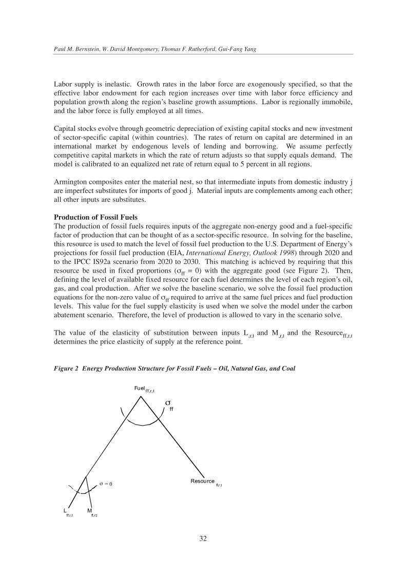
Labor supply is inelastic. Growth rates in the labor force are exogenously specified, so that theeffective labor endowment for each region increases over time with labor force efficiency andpopulation growth along the region’s baseline growth assumptions. Labor is regionally immobile,and the labor force is fully employed at all times.
Capital stocks evolve through geometric depreciation of existing capital stocks and new investmentof sector-specific capital (within countries). The rates of return on capital are determined in aninternational market by endogenous levels of lending and borrowing. We assume perfectlycompetitive capital markets in which the rate of return adjusts so that supply equals demand. Themodel is calibrated to an equalized net rate of return equal to 5 percent in all regions.
Armington composites enter the material nest, so that intermediate inputs from domestic industry jare imperfect substitutes for imports of good j. Material inputs are complements among each other;all other inputs are substitutes.
Production of Fossil Fuels The production of fossil fuels requires inputs of the aggregate non-energy good and a fuel-specificfactor of production that can be thought of as a sector-specific resource. In solving for the baseline,this resource is used to match the level of fossil fuel production to the U.S. Department of Energy’sprojections for fossil fuel production (EIA, International Energy, Outlook 1998) through 2020 andto the IPCC IS92a scenario from 2020 to 2030. This matching is achieved by requiring that thisresource be used in fixed proportions (σff = 0) with the aggregate good (see Figure 2). Then,defining the level of available fixed resource for each fuel determines the level of each region’s oil,gas, and coal production. After we solve the baseline scenario, we solve the fossil fuel productionequations for the non-zero value of σff required to arrive at the same fuel prices and fuel productionlevels. This value for the fuel supply elasticity is used when we solve the model under the carbonabatement scenario. Therefore, the level of production is allowed to vary in the scenario solve.
The value of the elasticity of substitution between inputs L,r,t and M,r,t and the Resourceff,r,tdetermines the price elasticity of supply at the reference point.
32
Paul M. Bernstein, W. David Montgomery, Thomas F. Rutherford, Gui-Fang Yang
σff
Resourceff,r ,t
Fuel ff,r,t
ff,r,tL
ff,r,tM
σ = 0
Figure 2 Energy Production Structure for Fossil Fuels – Oil, Natural Gas, and Coal

Household Behavior, Consumer Choice, and the Representative AgentFor each region, there is one infinitely-lived “representative” agent who chooses to allocate itsregion’s entire lifetime income across consumption in different time periods in order to maximizewelfare. In each period, the consumer faces the choice between current consumption and futureconsumption that is purchased via savings. The pure rate of time preference between current andfuture consumption determines the intertemporal allocation of consumption. In equilibrium, theagent is indifferent between consuming one unit of consumption today or consuming the value ofone unit of consumption that is adjusted for time preference tomorrow. We employ an intertemporalseparable utility function where the intra-period utility from consumption is based on a nested CESfunction over imported and domestic commodities. The representative agent maximizes utilitysubject to an intertemporal budget constraint.
The budget constraint equates the present value of consumption demand to the present value ofwage income, the value of the initial capital stock, and the present value of rents on fossil energyproduction, less the value of post-terminal capital. In this formulation savings are determinedimplicitly so as to equalize the marginal utility of a unit of investment and current consumption.Savings are used for future consumption.
Current consumption is a CES aggregate of energy and non-energy goods (see Figure 3). Consumerssubstitute between the end-use energy aggregate and the industry good aggregate with an elasticityof substitution σend. This elasticity varies over time to reflect capital stock turnover and the ease ofdeploying new technology. For OECD countries, this elasticity starts at a value of 0.35 in the year2000 and rises linearly to 0.6 in 2030; for non-OECD countries, it has an initial value of 0.3 andrises linearly to 0.5 over the 30-year time horizon. This elasticity approximately equals the own-price elasticity of demand for energy because energy represents only a small fraction of totalconsumption.
Aggregate end-use energy is composed of the fossil fuel aggregate. The aggregate comprises oil,gas, and coal; these fuels substitute against each other with an interfuel elasticity of substitutionequal to σfuel. Electricity is nested together with the non-energy goods. Each non-energy good inthe fuel nest is an Armington composite, in which domestic and imported goods are combined in themanner described below. Purchase of the good is financed from the value of the household’sendowments of labor, capital, energy-specific resources, and revenue from any carbon permit sales.
33
Effects of Restrictions on International Permit Trading: The MS-MRT model
Consumptionr,t
σend
σfuel
σgoods
Oil Gas Coal Y EIS ELE
Cr,tE Cr,t
I
Figure 3 Consumption Nest

International TradeTrade takes place in the fossil fuels and in the composite non-energy goods. All bilateral trade flowsfor the non-energy goods are represented in the MS-MRT model.
On the import side, consumers and industries choose between these domestically produced goodsand imports. Demands for imports stem from cost-minimizing producer behavior and utility-maximizing household behavior. For the non-energy goods, an Armington trade structure is usedso that the model differentiates between domestic and foreign goods. Therefore, domesticallyproduced goods and imports are imperfect substitutes. Small cost differences across regions for agood do not lead to a total shift in demand from one region to another, and small changes in costslead to small movements away from existing trade patterns. In addition, the Armington structureaccommodates both imports and exports of the same commodity across regions (cross-hauling). To create the Armington aggregate, imports of each non-energy good from each region substituteagainst each other with an elasticity of substitution equal to the Armington elasticity, σMM, and theaggregate import good substitutes against the comparable domestic good with an elasticity ofsubstitution (σDM) equal to half of σMM. The Armington elasticity σDM is set at 4 for this modelwith two non-energy goods because those composite goods are not likely to be identical acrosscountries. This elasticity measures how easily imports can substitute for domestically producedgoods. The Armington elasticity affects the potential gains in non-Annex I export sales that willoccur when lower energy costs give these non-participating countries a competitive advantage.Figure 4 displays this structure. Ai,r,t represents either consumer or industry demand for the non-energy good i in region r in time period t. Industries and consumers consume an Armingtonaggregate of domestically produced goods (Di,r,t) and goods imported (Mi,s,t) from regions s ≠ r.
The models incorporate international markets for all goods. For these goods, we have a globalmarket-clearing condition for the MS-MRT model:
r
rtj
r
rtj X = M t, j { }∑ ∑ ∀ ∈ energy goods, non - energy goods
34
Paul M. Bernstein, W. David Montgomery, Thomas F. Rutherford, Gui-Fang Yang
Dom. Goodi,r,t
s = r
Armington i,r,t
σMM
= 2* σDM
σDM
Import Goodi,s,t (Mi,s,t)
(Di,r,t)
/
Figure 4 Armington Nest Trade Structure for Consumption and Production

The model is closed with respect to international trade through the intertemporal budget constraint.The intertemporal budget constraint for the representative agent in each region requires that the netpresent value of international borrowing or lending remain equal to the baseline level over themodel’s time horizon. This implies that any change in capital flows must net to zero (in present
value terms) over the time horizon. Since the current account surplus or deficit (equal to the valueof net exports) equals net international lending or borrowing, this also implies that the net presentvalue of the change in the current account must be zero over the time horizon. The imposition ofan intertemporally balanced trade account is linked to an implicit exchange rate that reconciles thepresent value of each region’s domestic import demands with the present value of its exports.
This budget constraint allows changes in capital flows to play a part in determining the tradeimpacts of carbon limits. In contrast, the EPPA model assumes a period-by-period balance-of-payments constraint so that the current account deficit or surplus must equal baseline levels in eachyear. The G-Cubed model imposes a constraint on capital flows, so that a region’s net foreignindebtedness can change over the model time horizon. G- Cubed accounts for the effects of changesin indebtedness by calculating GNP, in which interest payments on foreign debt are deducted fromdomestic output (GDP).
Savings and Investment (Dynamics)MS-MRT is a fully dynamic general equilibrium trade model. The model structure incorporatesforward-looking investment and savings behavior, so that businesses, individuals, and governmentsanticipate the effects of announced policies that are to take effect in the future. The level of savingsand investment in a given period is endogenously determined by entrepreneurs and households thatmaximize the firm’s value and the representative agent’s lifetime consumption. Entrepreneurschoose investment levels to maximize the net present value of profits, and savings behavior isdetermined by intertemporal utility maximization. Therefore, investment dollars are placed in thearea where they will receive the highest return. Physical capital stocks depreciate at a constantgeometric rate, and they are incremented by investment from domestic output. The finite horizonposes some problems with respect to capital accumulation. In the absence of any terminaladjustment, agents would consume all capital stock in the terminal period and thus let the value ofthe capital stock decline to zero after 2030. This would have significant repercussions for rates ofinvestment in the periods leading up to the end of the model horizon. To correct for these effects,we apply an auxiliary equation dealing with the terminal capital stock.
It should be emphasized that we apply this side constraint along with the other economicequilibrium conditions (zero profit, market clearance, and income balance), but the application ofthis constraint has no implications for investment and consumption activities because these impactsdo not enter into the zero-profit conditions for these activities. Instead, we close the model byincluding a terminal capital stock variable, the quantity of which is determined so that the rate ofgrowth of terminal investment is balanced. That is, the shadow price of the above auxiliaryconstraint is the price of the terminal capital stock.
Carbon RestrictionsTo comply with the Kyoto Protocol, the model places a carbon emissions limit on the participatingcountries. The model endows these countries with emissions permits that allow them to emit carbonup to the level to which they agreed. In the MS-MRT model, it is assumed that, under the no-tradescenario, the emissions permits are tradable within each Annex I region but not across regions.Under the trading scenarios, emissions permits can be traded among the different blocs: for theAnnex I trading scenario, only Annex I countries face carbon limits, and the permits are tradable
35
Effects of Restrictions on International Permit Trading: The MS-MRT model

across all Annex I countries; for the global trading scenario, all countries face carbon limits, and thepermits are tradable throughout the world.3
Benchmarking and Calibration4
This section describes how the MS-MRT model was benchmarked and calibrated. As is customaryin applied general equilibrium analysis, the MS-MRT model is benchmarked to economictransactions in a particular year (1995). Benchmark data determine the parameters and coefficients(value shares) of the CES production, demand, and utility functions. Base-year finance statisticsindicate the value of payments to capital across sectors and the gross value of capital formation. Forcalibration, we needed to determine a reference level of emissions growth, GDP growth, energyproduction, energy, and non-energy trade. This entailed assigning values to key elasticities, such asend-use demand, Armington, oil supply, and the Autonomous Energy Efficiency Improvement(AEEI).
To develop a consistent database for energy and non-energy trade and input-output data, we mergednon-energy trade data, input-output data, and input-output coefficients for energy from the GTAPdatabase with data from the International Energy Agency (IEA). (See Babiker and Rutherford[1996] for details.)
For carbon emissions forecasts, the model was calibrated to the projections of both DOE and theInternational Panel on Climate Change. The reference or business-as-usual (BAU) level growthpath for world emissions is taken to be the IPCC’s reference scenario IS92A. The IS92A scenariocorresponds to the IPCC’s baseline (medium growth) scenario, which calls for worldwide carbondioxide emissions to grow from 6.0 billion tonnes in 1990 to 10 billion tonnes by the year 2020.The reference level emissions growth determines the amount of emissions reduction required tomeet the carbon limits called for by any carbon abatement policy.
The energy production and consumption forecasts as well as regional emissions were obtained fromthe Department of Energy’s International Energy Outlook, 1998. These forecasts were thencalibrated to current EIA data and the IS92A scenario so that energy consumption was consistentwith carbon emissions. The business-as-usual GDP growth rates were taken from MERGE (aModel for Evaluating the Regional and Global Effects of greenhouse gas reduction policies), whichwas developed by Alan Manne and Richard Richels.
Selecting Elasticity Values and Backstop PricesSelecting elasticity values affects the dynamics of the model and how the model responds under acarbon abatement policy. The choice of values has no effect on the baseline level of energyproduction and consumption, which is benchmarked through choice of other free parameters so thatthe chosen baseline is replicated as a market equilibrium. There are several key elasticities that needto be chosen for an MS-MRT simulation, including the oil supply price elasticity, Armingtonelasticity, end-use demand elasticity, interfuel elasticity of substitution, and the cost of the carbon-free backstop technology.
36
Paul M. Bernstein, W. David Montgomery, Thomas F. Rutherford, Gui-Fang Yang
3 In the MPS/GE framework in which MRT-MS is written, creating a market for carbon permits and imposing a cap on carbon emissionsfor each country is straightforward. See the web site, www.gams.com, for a description of the MPS/GE modeling language.
4 For further technical details on how the MS-MRT is benchmarked, see Bernstein, Rutherford and Montgomery, 1998.

Core Scenarios
For a point of reference, the MS-MRT model was run under three different emissions tradingscenarios: No trading, trading only among Annex I countries (Annex I trading), and full globaltrading (Global trading). These three trading regimes provide a basis for understanding theopportunity cost of restrictions on emissions, so we refer to them as the core scenarios. The firsttwo scenarios are possible outcomes of the Kyoto Protocol, unlike the third, which is impossiblegiven the Protocol’s current wording. Under Annex I and global trading, no restrictions on sales orpurchases of emissions permits were applied. Each Annex I region was assigned emissions limitsfor 2010 consistent with its obligation under the Protocol (see Table 2). Under the global tradingscenario, non-Annex I countries assume an emissions target equal to their emissions under the no-trading scenario.
Results for Core ScenariosIn the core scenarios, the MS-MRT model consistently finds that emissions limits on industrialcountries with no international emissions trading have negative impacts on the welfare of industrialand oil-producing countries, and both positive and negative welfare effects on energy-importingnon-Annex I countries (see Table 3). Annex I trading improves the situation for all regions, exceptChina and India, but only changes the sign for EE/FSU. All regions benefit under global trading ascompared to no trading; only EE/FSU is worse off under global trading than under Annex I trading.
37
Effects of Restrictions on International Permit Trading: The MS-MRT model
Table 2 Kyoto Protocol’s Emissions Targets for Annex I Regions
Region 2010 Target (% Change from 1990)
U.S. -7%Japan -6%Canada -6%European Union of 15 -8%Other OECD +1.1%EE/FSU -2%
Table 3 Welfare under the Three Benchmark Trading Cases (Percentage Change from Baseline)
Trading ScenariosRegions No Trading Annex I Global
USA -0.56% -0.36% -0.14%JPN -0.64 -0.23 -0.03EUR -0.45 -0.25 -0.05OOE -0.92 -0.76 -0.30SEA -0.18 -0.04 0.25OAS -0.10 -0.01 0.19CHI 0.34 0.22 0.34EE/FSU -0.42 4.44 0.48MPC -1.39 -1.15 -0.36ROW -0.10 -0.08 0.03

Carbon permit prices differ across regions when international permit trading is not permitted (Table4). Annex 1 trading lowers permit prices for all Annex 1 regions except the EE/FSU, which is thesole seller of permits. Global trading further lowers prices for Annex 1 regions, but raises permitand energy prices for non-Annex 1 regions.
Terms of trade generally move against developing countries and in favor of industrial countrieswhen developing countries do not participate in international emissions trading. This is becauseindustrial countries’ costs increase, driving up the price of their exports, and their incomes andimport demand fall, driving down the price of their imports. This is the reason for the negativewelfare impacts on developing countries noted above. Some developing countries (e.g., China) canoffset these terms-of-trade losses with industrial countries because of their gains in terms of tradewith OPEC and ability to shift to production of energy-intensive goods where they have increasedcomparative advantage over the industrial countries (see Table 5).
When non-Annex I countries do not participate in emissions trading, the shift of energy-intensiveindustries, from baseline levels, out of Annex I countries into non-Annex I countries is significant.
38
Paul M. Bernstein, W. David Montgomery, Thomas F. Rutherford, Gui-Fang Yang
Table 4 Carbon Permit Price under Three Benchmark Scenarios(1995 U.S. Dollars per Metric Ton)
Scenario Region 2010 2020 2030
No Trading USA $275 $314 $356JPN 468 523 526EUR 209 309 430OOE 249 363 505EE/FSU 0 10 49
Annex I Trading Annex I 90 151 225Global Trading World 31 36 32
Table 5 Terms of Trade under the Three Core Scenarios(Percentage Change from Baseline)
No Trading Annex I Global No Trading Annex I Global
Region 2010 2010 2010 2020 2020 2020
USA 0.04% -0.14% -0.08% -0.03% -0.14% -0.10%JPN 0.11 -0.05 -0.05 0.44 -0.01 -0.05EUR 0.02 0.04 -0.05 0.07 0.07 -0.06OOE 0.00 -0.08 -0.08 0.15 -0.09 -0.12SEA -0.27 -0.10 0.08 -0.29 -0.15 0.11OAS -0.14 0.04 0.09 -0.21 -0.02 0.09CHI -0.19 -0.04 0.44 -0.28 -0.14 0.57EE/FSU -0.44 1.71 0.27 -0.76 1.99 0.23MPC -0.60 -0.44 0.10 -0.89 -0.69 0.05ROW 0.28 0.22 0.13 0.13 0.18 0.08

Annex I emissions trading moderates the shift of industry by reducing production costs in mostAnnex I countries. Interestingly, the U.S. and EE/FSU, the lowest-cost providers of permits, sufferthe greatest losses in their energy-intensive industries under Annex I trading. With global trading,production from non-Annex I energy-intensive industries declines from the levels it reaches underno trading and Annex I trading. For a subset of these countries and in certain time periods, someEIS production relocates to Annex I countries as reported by the negative percentage changes inTable 6. This occurs because the GTAP data show that many of the Non-OECD countries have theleast energy-efficient industries and, therefore, are the most vulnerable to a uniform, global increasein energy costs (see Table 6).
Carbon leakage is also significant. It is connected with shifts in energy-intensive industries, reducedenergy efficiency, and fuel substitution due to lower fuel prices in developing countries (see Table7). Leakage is affected very little by Annex I trading, because it arises mostly from differences inenergy prices between Annex 1 and non-Annex 1 countries. With Annex I trading, global emissionsalso increase because of hot air sales by EE/FSU, increasing apparent leakage to developingcountries in percentage terms. Global trading, by definition, eliminates leakage because all regionsface emissions caps.
Table 8 illustrates that there is a direct relationship between the spillover effects as measured bycarbon leakage and the number of non-energy sectors included in the model. Dis-aggregating thenon-energy sectors allows for more heterogeneity among these sectors and hence more and better
39
Effects of Restrictions on International Permit Trading: The MS-MRT model
Table 6 Output from Energy-Intensive Industries in 2010 and 2020(Percentage Change from Baseline)
No Trading Annex I Global No Trading Annex I Global
Region 2010 2010 2010 2020 2020 2020
USA -7.87% -2.43% -0.59% -7.66% -3.62% -0.51%JPN -1.06 0.10 0.18 -1.82 -0.15 0.15EUR -0.17 0.50 0.44 -1.56 0.33 0.45OOE -2.69 -0.32 0.35 -5.98 -1.04 0.50SEA 4.69 2.01 0.07 4.21 2.55 -0.06OAS 2.51 0.56 0.07 2.26 0.87 0.12CHI 1.94 0.89 -0.57 2.01 1.32 -0.85EE/FSU 5.87 -10.22 -2.98 6.42 -13.93 -2.78MPC 4.67 2.51 -0.15 5.65 4.10 0.04ROW 1.32 0.52 -0.04 1.53 0.89 0.03
Table 7 Carbon Leakage under No Trading and Annex I Trading Regimes (Change in Non-Annex I Emissions Divided by Change in Annex I Emissions)
2010 2015 2020 2025 2030
No Trading 18 19 20 21 21Annex I Trading 16 18 19 21 22

opportunities for countries to shift production between energy-intensive industries and industriesthat use little energy. As the number of non-energy sectors increases from one to two to four, theratio in energy-intensity for the U.S. among the non-energy sectors increases from one to 3.4 to 6.8,respectively. Therefore, with more non-energy sectors, the Annex I countries have more incentiveto decrease production in their most energy-intensive industries and import these goods from non-Annex I countries which now have a greater competitive advantage.
The results in Table 8 would be more dramatic if the Armington elasticities varied across the cases.In theory, the Armington elasticities should be smaller with fewer sectors since goods are moreaggregated and hence poorer substitutes. As one moves to more sectors so that goods are closersubstitutes, the Armington elasticity should increase. Increasing the Armington elasticity as oneincreases the number of non-energy sectors would magnify the difference among leakage rates fromthose in Table 8.
Measures of Welfare
There are a number of alternative measures of economic impacts that appear in different studies:change in consumers’ surplus measured by the equivalent variation, the discounted present value ofconsumption (DPVC), GDP, and direct cost. In general, for an optimization model there is onetheoretically consistent measure, which is based on the value of the objective function maximizedin the model. In our model, this measure is the intertemporal equivalent variation.5 If we hadimplemented this model with an infinite horizon (difficult computationally), changes in welfarecould be taken directly from the value of the intertemporal utility function. Since we terminate themodel in 2030, we must add to the utility experienced during the period an adjustment thatrepresents the change in the value of the terminal capital stock that is left for future generations.This adjustment makes our calculation of the infinite horizon welfare approximate, because to valuethe terminal capital stock we need to employ some assumptions about how close the temporaryequilibrium in 2030 is to one on a balanced growth path.
The same issue about terminal capital stock applies to calculating the discounted present value ofconsumption as a welfare measure. These considerations about the terminal capital stock are
40
Paul M. Bernstein, W. David Montgomery, Thomas F. Rutherford, Gui-Fang Yang
Table 8 The Effect of Carbon Leakage under Different Aggregations (2010 for No Trading and Annex I Trading Regimes)
Number of Non-Energy Sectors
Scenario 1 2 4
No Trading 16.2 17.9 19.3Annex I Trading 15.1 15.8 16.5
5 For a discussion of how this welfare measure is computed in the MRT-MS, see Thomas F. Rutherford, "Constant Elasticity ofSubstitution Functions: Some Hints and Useful Formulae," Notes prepared for GAMS General Equilibrium Workshop, held December1995, in Boulder, Colorado; available from http://www.gams.com/solvers/mpsge/cesfun.htm. For a general discussion of this welfaremeasure, see Hal Varian, Microeconomic Analysis, Third Edition, New York, 1992, pp. 160-171.

important, because emissions limits produce large drops in investment (as high as 2.5 percent underno trading in the U.S.), which imply very different capital stocks in 2030 in the baseline and thepolicy cases. Agents buffer consumption during the shock period by reducing investment, and theeffects of this reduced investment on their future welfare need to be taken into account.
GDP, the other common measure, has classic index number problems, that in our model appear insensitivity of the results to choice of numeraire. GDP includes both consumption and investment,so that over short periods of time GDP may increase due to a stimulus to investment even thoughconsumption falls. In addition, GDP is a measure of gross, not net, income, in the sense that it doesnot account for depreciation of capital. When policies lead to large reductions in investment for asustained period of time, they lead to lower levels of capital stock and to reduced capitalconsumption allowances (CCA). As a result, GDP falls because of both contemporaneousreductions in investment and lower CCA. This effectively double-counts the reduction ininvestment and produces a larger percentage reduction in GDP than in net national income. GDPalso fails to account for net interest payments on foreign debt, so that if a policy causes a significantchange in foreign debt, GDP will inaccurately measure the change in real income for residents of acountry.6
Finally, it is possible to produce an approximate measure of the direct cost of a policy by estimatingthe area under the curve for the marginal cost of carbon abatement. This measure equals one-halfthe carbon tax times the reduction in emissions plus the net receipts or payments for internationalpermits. Some models (e.g., the SGM) use this measure.7
The values of these different measures are provided in Table 9. GDP and “direct cost” are all annualmeasures, while EV and discounted present value of consumption are present value measures.Thus, we present GDP and “direct cost” for different years (2010 and 2020) and welfare and DPVCas a single number. For welfare, DPVC, and GDP, the numbers report the percentage change frombaseline numbers whereas direct cost reports the cost in units of billions of 1995 U.S. dollars.8
Comparing these measures illuminates three critical issues. First, one measure can imply a countrybenefit under a specific scenario while another measure implies a loss. Second, the measures canproduce different policy rankings for a specific region. Third, the magnitudes of these measures areincomparable unless all of them are in the same units (see Table 10).
Table 9 points out the problems of reporting welfare measures that are not directly connected to themodel’s objective function. As mentioned, for our model, equivalent variation of welfare is the onlyself-consistent welfare measure. In general, DPVC closely approximates welfare, but the signdiffers for ROW in the no trading and Annex I trading scenarios and for SEA under the Annex Itrading scenario. This inconsistency arises because of the difference between the implicit discountrate (intertemporal rate of substitution) in the welfare function and the specified discount rate forDPVC.
For Annex I countries, the direct cost is consistent with equivalent variation (welfare) both withinand across emissions trading scenarios. But this measure reveals little about the welfare of non-Annex I countries because it leaves out the terms-of-trade effects that are responsible for spillover
41
Effects of Restrictions on International Permit Trading: The MS-MRT model
6 William Nordhaus deserves the credit for this observation.7 This measure is reported by the SGM and in the Administration’s economic analysis of the Kyoto Protocol. See "The Kyoto Protocoland the President's Policies to Address Climate Change," Administration Economic Analysis, July 1998; and J.A. Edmonds, et al.,"Return to 1990: The Cost of Mitigating United States Carbon Emissions in the Post-2000 Period," October 1997. 8 Costs are reported as negative numbers.

effects. Furthermore, under global trading, direct cost reports a gain for MPC, but MPC experiencesa loss in welfare due to the fall in world oil prices.
Comparing GDP results among countries or across scenarios may not present a clear picture ofwhether one country does better compared to another, or whether a particular scenario is beneficialfor a country because the change in GDP may be positive in one period but negative in the next.Also, to compute GDP, one needs a numeraire; there is no theoretically correct choice for this.Therefore, depending on the choice of numeraire, one arrives at different results for GDP. This leadsto some of the inconsistencies when comparing impacts on CHI across scenarios. Using GDP asthe welfare measure, CHI is better off under no trading and Annex I trading than under globaltrading, whereas EV (welfare) implies the opposite conclusion. This problem arises whencomparing results for many of the non-Annex I, non-energy exporting regions and is due to the largechanges in investment that increase GDP in some countries for a period of time at the expense ofconsumption.
42
Paul M. Bernstein, W. David Montgomery, Thomas F. Rutherford, Gui-Fang Yang
Table 9 Comparison of All Four Welfare Measures for Selected Regions
Welfare DPVC Direct Cost GDP
2010 2020 2010 2020
No Trading (%) (%) (Billions of U.S. $s) (%) (%)USA -0.56% -0.41% -$45.20 -$43.55 -1.88% -2.33%SEA -0.18 -0.03 NA NA 0.51 0.01CHI 0.34 0.59 NA NA 0.64 0.21MPC -1.39 -1.65 NA NA -0.99 -1.60ROW -0.10 0.10 NA NA 0.71 0.17Annex IUSA -0.36 -0.31 -36.39 -57.53 -0.91 -1.27SEA -0.04 0.04 NA NA 0.47 0.50CHI 0.22 0.33 NA NA 0.53 0.60MPC -1.15 -1.45 NA NA -0.64 -0.91ROW -0.08 0.01 NA NA 0.60 0.60GlobalUSA -0.14 -0.14 -15.41 -21.91 -0.29 -0.33SEA 0.25 0.36 1.33 2.63 0.06 0.02CHI 0.34 0.52 4.55 13.58 -0.17 -0.07MPC -0.36 -0.42 1.40 3.02 -0.45 -0.48ROW 0.03 0.08 2.42 5.02 0.06 0.04
Table 10 Comparison of Four Welfare Measures for the U.S. (Percentage Change from Baseline – Cumulative and Discounted to 2000)
Scenario EV (Welfare) DPVC Direct Cost GDP
No Trading -0.56% -0.41% -0.19% -1.31%Annex I Trading -0.36 -0.31 -0.07 -0.75Global Trading -0.14 -0.11 -0.01 -0.18

The magnitudes of the welfare measures as reported in Table 9 are not directly comparable. GDPand direct cost are annual measures, whereas EV welfare and DPVC measure the discounted presentvalue of impact over a horizon. Furthermore, the units of direct cost are dollars. To eliminate thesedifferences, we computed the discounted PV of the direct cost and GDP for the scenarios over thefull time horizon. Then, to compute the percentage change from baseline, these are divided by theDPV of the baseline GDP (see Table 10). The EV Welfare still differs from the other measures sinceit approximates the impacts over the infinite horizon rather than the model’s 30-year horizon.
The GDP measure shows the largest impacts, partly because of the double counting of investmentimpacts noted above. Direct cost shows the smallest impacts since it leaves out effects oninvestment, terms of trade, and other general equilibrium effects, and also because it is not based onthe compensated demand curve required theoretically to approximate consumer surplus. Welfareand DPVC are close, with slight differences caused by discrepancies between the discount rateassumed in calculating the DPVC and the internal discount rate used in the welfare calculation. TheEV welfare measure could be closer to GDP if its denominator were limited to welfare during themodel horizon, rather than the infinite horizon.
Restricted Trading Cases
The Kyoto Protocol did not reconcile the positions of the U.S. and other Annex I nations onemissions permit trading. Three unresolved issues are especially important: 1) the extent to whicha country may satisfy its obligation through permit purchases, 2) the amount of paper tons or permitsfor “hot air”9 EE/FSU countries will be allotted, and 3) how market power will be exercised. Twoother questions also arise: What will be the economic impacts of restricting the sales of emissionspermits, and what will be the potential benefits to the Annex I countries of instituting the CDM?
To address the first three issues, we consider several different Annex I trading regimes. First, weconsider three regimes in which Annex I regions are limited in how many permits they can purchase.Proponents of restricted emissions trading cite the Kyoto Protocol language that trading should be“supplementary” to domestic efforts in support of these limits. The EU and several of its membercountries have proposed that a “concrete ceiling” be imposed on the percentage of a country’semissions obligation that may be satisfied through the purchase of emissions permits. Thesecountries have suggested a limit of 50 percent or less. In addition, some have advocated a systemof buyer liability that would so burden buyers of permits with potential liabilities that only the mostattractive trades would have any likelihood of being accomplished.
In our scenarios, the limits are set at 10 percent, 30 percent, and 50 percent of each country’sobligation. A country’s obligation is defined to be the difference between its baseline emissions andits target under the Kyoto Protocol. Since the limits are placed only on the demand side, countriescan sell as many permits as they like but are restricted by how much of their commitment they cansatisfy through the purchase of permits. We also consider a case in which a 50 percent limit existsunder a global trading system, since it is under global trading that our benchmark results suggestthat the U.S. would want to purchase more permits than this limit would allow.
43
Effects of Restrictions on International Permit Trading: The MS-MRT model
9 This positive difference between the EE/FSU’s Kyoto emissions targets and its actual forecasted emissions is referred to as "hot air"or "paper tons." Because the EE/FSU’s economy has been in a decline since 1990, its carbon emissions are forecasted to be below its1990 emissions level until somewhere in the 2020 to 2025 time period.

Second, we consider the impacts of prohibiting the EE/FSU region from selling its “hot air.” Russia,and possibly some of the former Soviet Republics and other Eastern European countries, will clearlybe the least-cost suppliers of permits in an Annex I trading system in 2010. Because its economiccollapse has reduced current emissions to levels well below its 1990 baseline, Russia’s emissions in2010 are projected to be about 20 percent below its Kyoto target.10
Most of the members of the EU, and many developing countries, are opposed to a system that allowsRussia to sell its hot air, arguing correctly that hot air sales would raise total world emissions abovethe levels they would reach without such sales11. Table 11 helps illustrate the concept of hot air.The line titled “Baseline” shows that, until 2020, EE/FSU’s emissions are below its Kyoto target of1990 emissions levels (“Kyoto Target” line). This gap between the region’s Baseline emissions andits target (line titled “Kyoto Target”) is referred to as “hot air.” In 2010, the EE/FSU is forecastedto have about 220 million metric paper tons. In the No Hot Air case, EE/FSU is restricted fromselling their paper tons of carbon. Under this case, EE/FSU’s emissions target is denoted by the “NoHot Air” line, which equals the smaller of EE/FSU’s business-as-usual emissions or its Kyoto targetof the1990 emissions level. Therefore, under the Annex I trading regime, the emissions cap for theentire Annex I bloc is lower under the No Hot Air case than under the other cases.
Third, we address the issue of market power. As the only net seller of permits under a tradingsystem limited to Annex I countries, Russia would be in a position to restrict output and chargemonopoly prices for its emissions permits. We consider one scenario in which EE/FSU is able toexercise some market power. We also describe a method for estimating the output restriction thatwould maximize benefits to EE/FSU and the resulting prices. This case is intended to provide anillustration of how monopoly power could be exercised if Eastern Europe and the FSU maximizeprofits jointly.
Fourth, we consider other restrictions on sales. We analyze a case where countries are allowed tosell only 30 percent of the permits that they would sell under unrestricted Annex I trading. This caseis designed to examine whether proposed restrictions on sales would achieve the same result asexercise of monopoly power, and whether restrictions on sales could produce worse outcomes thanunilateral exercise of monopoly power.
Finally, we examine how closely the CDM approximates the benefits of full global trading. CDMis designed to support projects to reduce emissions from developing countries, with funding fromindustrial countries that would receive emission credits. We limit permit sales from each of the non-Annex I regions to 15 percent of their total permit sales under full global trading. This differs from
44
Paul M. Bernstein, W. David Montgomery, Thomas F. Rutherford, Gui-Fang Yang
Table 11 EE/FSU’s Carbon EmissionsTargets(Millions of Metric Tons)
2000 2005 2010 2015 2020 2025 2030
Baseline 870 940 1,023 1,094 1,174 1,267 1,371Kyoto Target N/A N/A 1,240 1,240 1,240 1,240 1,240Hot Air N/A N/A 217 146 66 0 0No Hot Air N/A N/A 1,023 1,094 1,174 1,240 1,240
10 U.S. Department of Energy, International Energy Outlook, 1998.
11 This assumes no banking of carbon emissions by EE/FSU.

full global trading because it leaves most of the price differentials between Annex I and non-AnnexI countries in place.
Modeling of Restricted Trading CasesTo model restricted trading in the framework of complete markets, one needs to create markets forimport and export quota coupons in addition to markets for permits. The permit is a normal tradedgood, subject to a nontradable quota. These coupons must be used when either importing orexporting emissions permits. In the case of unrestricted permit trading, every region is endowedwith an excess of quota coupons so that the price of coupons is zero. In the restricted trading cases,however, each region that is a member of the trading bloc is endowed with a fixed number of quotacoupons equal to the limit of its restriction. For example, if the final version of the Protocol wereto limit each Annex I country’s permit purchases to 30 percent of its obligation, then each countrywould be given quota coupons equal to 30 percent of its obligation. Restricting permit sales worksthe same way except, now, sellers must use quota coupons to vend permits.
Under the CDM case, the non-Annex I countries are allowed to sell 15 percent of their permits thatthey would have sold under the unrestricted global trading case. This is a modeling convenienceand could not be implemented in reality. But this case serves to estimate the effect of implementingthe CDM in a way that would allow non-Annex I countries to participate in the process of reducingglobal emissions, but with costs and restrictions that render 85 percent of the trades possible underglobal trade no longer economic. To model this proxy for the CDM, the non-Annex I countries areendowed with quota coupons equal to 15 percent of their emissions permit sales under unrestrictedglobal trading. There are no restrictions on permit trading among Annex I regions.
By treating limits on purchases and sales of emissions permits as, respectively, import and exportquotas, the international price of permits is set by the holder of the quota coupons. Therefore, whenpurchases are restricted, the international price is determined by the market supply curve forpermits; but when the sales are limited, the international price is determined by the market demandcurve for permits.
Modeling Russian Exercise of Monopoly PowerBecause EE/FSU is the sole seller under Annex I trading, the potential arises for this group ofcountries to exercise market power. To estimate the possible effects of this event, we allow theEE/FSU to maximize its welfare by selling permits above competitive price levels. In the MS-MRTmodel, a markup is added to the EE/FSU’s domestic price of permits, much like an export tariff.Other Annex I regions pay the EE/FSU this marked-up price. The markup drives a wedge betweenthe price received by sellers of permits in Russia and the price received by Russia on theinternational market. The markup thus reduces the EE/FSU’s incentive to sell permits and(consistent with standard trade theory) has the same effect as a quota on the sales of permits (seeFigure 5).
To analyze whether the EE/FSU could benefit from acting as a monopolist, we imposed differentmarkups on the price of permits offered for sale by the EE/FSU. This treatment is similar to lettinga country charge a tariff where the country captures all the revenues from the levy. In order todetermine the optimal tariff (the one that maximizes EE/FSU’s welfare), we investigated severalmarkup formulas. Intuitively, the optimal tariff should decline over time as the EE/FSU’s baselineemissions increase relative to its target and the difference between the OECD’s marginal cost ofabatement and that of the EE/FSU decreases. From the tariffs tried, the following markup scheduleyielded the greatest welfare gains for EE/FSU: 180% in 2010 declining to 18% in 2030.
45
Effects of Restrictions on International Permit Trading: The MS-MRT model

Modeling of No Hot AirIn this scenario, EE/FSU is prohibited from selling permits that are the result of hot air.Equivalently, EE/FSU’s emissions target becomes the lesser of its baseline emissions and its Kyototarget. For the period 2010 to 2020, EE/FSU’s new emissions target equals its baseline emissions.After 2020, its target reverts back to its assigned target under the Kyoto Protocol – its 1990emissions level (see Line titled “No Hot Air” in Table 11).
Results for Restricted Trading CasesThis section reports results for three different sets of restrictions. First, restrictions on Annex Itrading are compared to the case of unrestricted Annex I trading. Second, the effect of EE/FSUexercising market power and restricting permit sales is examined. Third, the impacts of imposingtrade restrictions under the global trading regime are studied.
Restricted Annex I Trading Scenarios
This section presents the results from the five Annex I restricted trading scenarios. These results arecompared to the unrestricted Annex I trading scenario. Trading is restricted in three different ways:purchases, sales, and allowable permits. Three scenarios that limit purchases are considered. Thelimits are set at 10 percent, 30 percent, and 50 percent of each country’s obligation. These scenariosare named, respectively, Annex I-10B, Annex I-30B, and Annex I-50B. One scenario (Annex I-30S)considers limits on sales where Annex I countries are allowed to sell only 30 percent of the permitsthat are assigned to them which equals 30 percent of their Kyoto targets. Finally, in the policy “NoHot Air,” we consider the impacts of prohibiting the EE/FSU region from selling its “hot air.”
Table 12 displays the range in welfare impacts under the different trading regimes. For the OECDcountries, unrestricted Annex I trading is better than either the Annex I-10B, Annex I-30S, or NoHot Air scenarios. Depending on the region’s marginal cost of abatement, its welfare under AnneI-30B (USA, OOE) or Annex I-50B (EUR) exceeds that in the unrestricted Annex I scenario. While
46
Paul M. Bernstein, W. David Montgomery, Thomas F. Rutherford, Gui-Fang Yang
4.40
4.45
4.50
4.55
4.60
4.65
4.70
0% 50% 100% 150% 200% 250% 300%
Carbon Permit Price Mark Up in 2010
Ch
ang
e in
Wel
fare
of
EE
/FS
U R
elat
ive
to B
asel
ine
(%)
Figure 5 Optimal Permit Price Markup in 2010 for EE/FSU(Percentage Increase from EE/FSU’s Domestic Price)
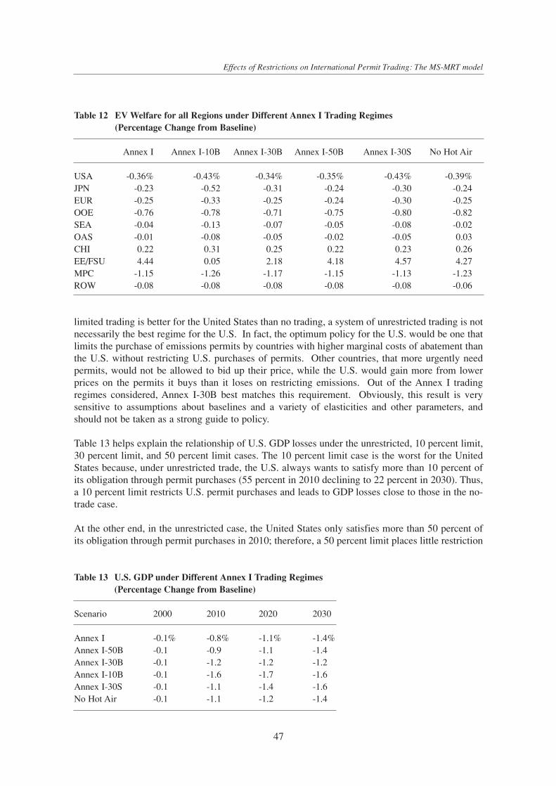
limited trading is better for the United States than no trading, a system of unrestricted trading is notnecessarily the best regime for the U.S. In fact, the optimum policy for the U.S. would be one thatlimits the purchase of emissions permits by countries with higher marginal costs of abatement thanthe U.S. without restricting U.S. purchases of permits. Other countries, that more urgently needpermits, would not be allowed to bid up their price, while the U.S. would gain more from lowerprices on the permits it buys than it loses on restricting emissions. Out of the Annex I tradingregimes considered, Annex I-30B best matches this requirement. Obviously, this result is verysensitive to assumptions about baselines and a variety of elasticities and other parameters, andshould not be taken as a strong guide to policy.
Table 13 helps explain the relationship of U.S. GDP losses under the unrestricted, 10 percent limit,30 percent limit, and 50 percent limit cases. The 10 percent limit case is the worst for the UnitedStates because, under unrestricted trade, the U.S. always wants to satisfy more than 10 percent ofits obligation through permit purchases (55 percent in 2010 declining to 22 percent in 2030). Thus,a 10 percent limit restricts U.S. permit purchases and leads to GDP losses close to those in the no-trade case.
At the other end, in the unrestricted case, the United States only satisfies more than 50 percent ofits obligation through permit purchases in 2010; therefore, a 50 percent limit places little restriction
47
Effects of Restrictions on International Permit Trading: The MS-MRT model
Table 12 EV Welfare for all Regions under Different Annex I Trading Regimes (Percentage Change from Baseline)
Annex I Annex I-10B Annex I-30B Annex I-50B Annex I-30S No Hot Air
USA -0.36% -0.43% -0.34% -0.35% -0.43% -0.39%JPN -0.23 -0.52 -0.31 -0.24 -0.30 -0.24EUR -0.25 -0.33 -0.25 -0.24 -0.30 -0.25OOE -0.76 -0.78 -0.71 -0.75 -0.80 -0.82SEA -0.04 -0.13 -0.07 -0.05 -0.08 -0.02OAS -0.01 -0.08 -0.05 -0.02 -0.05 0.03CHI 0.22 0.31 0.25 0.22 0.23 0.26EE/FSU 4.44 0.05 2.18 4.18 4.57 4.27MPC -1.15 -1.26 -1.17 -1.15 -1.13 -1.23ROW -0.08 -0.08 -0.08 -0.08 -0.08 -0.06
Table 13 U.S. GDP under Different Annex I Trading Regimes(Percentage Change from Baseline)
Scenario 2000 2010 2020 2030
Annex I -0.1% -0.8% -1.1% -1.4%Annex I-50B -0.1 -0.9 -1.1 -1.4Annex I-30B -0.1 -1.2 -1.2 -1.2Annex I-10B -0.1 -1.6 -1.7 -1.6Annex I-30S -0.1 -1.1 -1.4 -1.6No Hot Air -0.1 -1.1 -1.2 -1.4

on the U.S. and only limits the purchase of permits by other Annex I regions. As a result, the demandfor permits declines and the price drops relative to the regime of unrestricted Annex I trading.Therefore, the permit price to the U.S. under the 50 percent case is always less than or equal to theprice under the unrestricted case (see Tables 14).
Applying this analysis to the 30 percent case explains why, after 2015, the minimum weighted-average permit price12 for the United States occurs under the 30 percent limit case. After 2015, thiscase places no restrictions on the U.S.’s purchase of permits. But it does limit Europe and the OECDregions from purchasing as many permits as they would like; hence, they do not bid up the price ofpermits as high as in the 50 percent case. In the 30 percent case, the EE/FSU sells fewer permitsand, hence, their marginal cost of abatement is lower than in the 50 percent case. Consequently, after2015 the U.S. pays the least for emissions permits under the 30 percent limit case — less even thanunder the 50 percent case, because the demand for permits by other Annex I countries is restrictedwhile the U.S. demand is unaffected. This translates directly into less GDP loss for the United Statesunder the 30 percent case than under any of the other Annex I trading cases.
Currently, the U.S. government is advocating unrestricted emissions trading while many Europeancountries are calling for at least 50 percent of emissions reductions to be achieved through domesticactions. Interestingly, the above results show that the United States and the EU would stand tobenefit most from what the other wants: the U.S. would experience smaller GDP losses with limitedtrading, while the EU would benefit more from unrestricted trading.
Restricting the EE/FSU’s sale of hot air reduces the pool of emissions permits in the years 2010 to2020. Therefore, the price of permits under this case is higher during that period than under theunrestricted case. After 2020, the EE/FSU has no more hot air, and the pool of emissions permits isidentical under the no hot air and unrestricted cases. This leads to nearly identical carbon permitprices and GDP losses.
48
Paul M. Bernstein, W. David Montgomery, Thomas F. Rutherford, Gui-Fang Yang
Table 14 International and U.S. Domestic Price of Carbon Permits(1995 U.S. Dollars per Metric Ton)
Scenario International Permit Price U.S. Domestic Permit Price($ per Metric Ton) ($ per Metric Ton)
2010 2020 2030 2010 2020 2030
Annex I $90 $151 $225 $90 $151 $225Annex I-50B 72 150 225 104 150 225Annex I-30B 27 95 201 159 178 201Annex I-10B 0 33 89 230 263 293Annex I-30S 123 193 275 123 193 275No Hot Air 130 164 227 130 164 227
12 The Annex B weighted average permit price equals the price of international permits times the number of international permitspurchased plus the price of domestic permits times the number of domestic permits purchased all divided by the total number of permitspurchased.

Sensitivity Analysis of Results to Assumptions about Elasticity ValuesTo determine the robustness of the results about the benefits of unrestricted trading over restrictedtrading, we varied the values of the Armington (Arm) elasticities and the elasticity between energyand value-added (Esub) in the production and consumption nests. Raising the value of theArmington elasticity reduces the magnitude of price changes needed to induce countries tosubstitute between domestically produced goods and imports. In general, higher values ofArmington elasticities will allow non-Annex I countries to capture more export markets and willcause Annex I countries to lose market share in the export markets in the presence of carbonabatement policies. Raising the value of Esub makes it easier for producers and consumers tosubstitute energy for non-energy in production and consumption, respectively. Table 15 presents thedifference in the percentage change in welfare between the unrestricted Annex I trading scenarioand the 10 percent permit purchase restricted Annex I trading scenario under different elasticityassumptions.
Under the Low Arm-High Esub case, the U.S. is actually better off if permit purchases are restrictedto 10 percent of a country’s obligation rather than being unrestricted. These results occur becauseof the shape of the U.S.’s marginal cost curve relative to that of the OECD’s aggregate marginal costcurve and the EE/FSU’s supply curve. Under the other elasticity assumptions, the expected resultthat restricted trading hurts the U.S. appears. This sensitivity analysis emphasizes the importanceof particular elasticity values in evaluating restricted trading regimes.
Russian Exercise of Monopoly Power
To analyze Russia’s ability to exercise monopoly power, we run the global model repeatedly withdifferent markups and then choose the markup under which Russia’s welfare is maximized. Table16 reports this markup and the carbon prices under this markup schedule. For comparison, Table16 also states the international carbon price in the competitive Annex I trading scenario. The sizeof the markup (or export tariff) determines the restriction on Russian sales. As the markup decreasesover time, EE/FSU sells more permits (see Figure 5 and Table 16).
49
Effects of Restrictions on International Permit Trading: The MS-MRT model
Table 15 Welfare Differences under Different Elasticity Assumptions(Percent Change in Welfare in the Annex I Case Less That in Annex I-10B Case)
Region High Arm- High Arm- Low Arm-Low Esub Med. Esub High-Esub
USA 0.092% 0.068% -0.025%JPN 0.291 0.287 0.236EUR 0.072 0.083 0.053OOE 0.003 0.024 0.048SEA 0.095 0.082 0.070OAS 0.080 0.066 0.029CHI -0.104 -0.091 -0.066EE/FSU 4.890 4.389 4.265MPC 0.081 0.118 0.266ROW -0.019 0.000 0.030

In 2010, the optimal markup is about 180 percent (see Figure 5), implying that it could be inRussia’s interest to restrict sales by as much as 150 million metric tons (see Figure 6) and raiseprices by $39 per metric ton above competitive levels (rising from $90 to $129 per tonne). Permitprices in Russia would be driven down to $46 per tonne (see Table 16). Given the assumptionsunderlying the MS-MRT model, the demand curve for permits is relatively flat at this point, so thatEE/FSU must restrict output considerably in order to raise prices.
In this calculation, Russia is a very sophisticated monopolist, taking into account not only thenormal calculation of a price that maximizes revenue given demand elasticities, but the effects ofhigher permit prices on economic performance of Russia’s trading partners and the resultingfeedback effects on Russia. This is the same sophistication that analysts speculated that SaudiArabia showed during the 1970s in moderating oil price increases.
We also carried out a partial equilibrium analysis by using repeated model runs to construct a supplycurve for permits from Russia and a demand curve for permits in the rest of the Annex I. Themonopoly solution is where marginal revenue equals the supply curve. Figure 7 shows that thispartial equilibrium analysis predicts higher prices in both the competitive and monopoly cases forAnnex I trading than does the general equilibrium analysis, but the output restriction and priceincrease are about the same.
50
Paul M. Bernstein, W. David Montgomery, Thomas F. Rutherford, Gui-Fang Yang
Table 16 Permit Price under Monopolistic and Competitive Annex I Trading
2010 2015 2020 2025 2030
International Permit Price - Monopoly ($/tonne) 129 150 172 195 239EE/FSU Domestic Permit Price ($/tonne) 46 79 119 160 202International Carbon Price – Competitive Market ($/tonne) 90 119 151 182 225Mark-up (%) 180 90 45 23 18
300
350
400
450
500
550
2010 2015 2020 2025 2030
Per
mit
s S
old
(M
illio
ns
of
Met
ric
To
ns)
Free M arket
Compet itive Market
Figure 6 EE/FSU Permit Sales under Monopoly and Competitive Market Scenarios
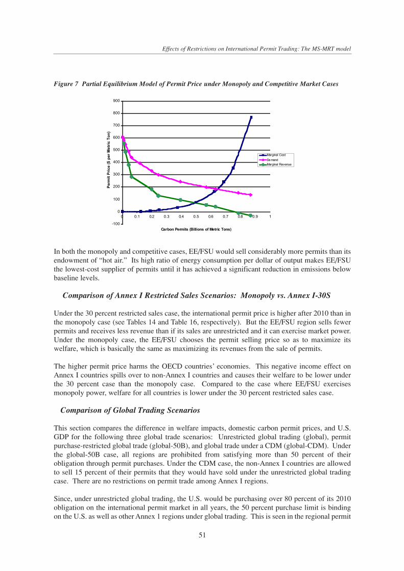
In both the monopoly and competitive cases, EE/FSU would sell considerably more permits than itsendowment of “hot air.” Its high ratio of energy consumption per dollar of output makes EE/FSUthe lowest-cost supplier of permits until it has achieved a significant reduction in emissions belowbaseline levels.
Comparison of Annex I Restricted Sales Scenarios: Monopoly vs. Annex I-30S
Under the 30 percent restricted sales case, the international permit price is higher after 2010 than inthe monopoly case (see Tables 14 and Table 16, respectively). But the EE/FSU region sells fewerpermits and receives less revenue than if its sales are unrestricted and it can exercise market power.Under the monopoly case, the EE/FSU chooses the permit selling price so as to maximize itswelfare, which is basically the same as maximizing its revenues from the sale of permits.
The higher permit price harms the OECD countries’ economies. This negative income effect onAnnex I countries spills over to non-Annex I countries and causes their welfare to be lower underthe 30 percent case than the monopoly case. Compared to the case where EE/FSU exercisesmonopoly power, welfare for all countries is lower under the 30 percent restricted sales case.
Comparison of Global Trading Scenarios
This section compares the difference in welfare impacts, domestic carbon permit prices, and U.S.GDP for the following three global trade scenarios: Unrestricted global trading (global), permitpurchase-restricted global trade (global-50B), and global trade under a CDM (global-CDM). Underthe global-50B case, all regions are prohibited from satisfying more than 50 percent of theirobligation through permit purchases. Under the CDM case, the non-Annex I countries are allowedto sell 15 percent of their permits that they would have sold under the unrestricted global tradingcase. There are no restrictions on permit trade among Annex I regions.
Since, under unrestricted global trading, the U.S. would be purchasing over 80 percent of its 2010obligation on the international permit market in all years, the 50 percent purchase limit is bindingon the U.S. as well as other Annex 1 regions under global trading. This is seen in the regional permit
51
Effects of Restrictions on International Permit Trading: The MS-MRT model
-100
0
100
200
300
400
500
600
700
800
900
0 0.1 0.2 0.3 0.4 0.5 0.6 0.7 0.8 0.9 1
Carbon Permits (Billions of Metric Tons)
Per
mit
Pri
ce (
$ p
er M
etri
c T
on
)
Marginal Cost
DemandMarginal Revenue
Figure 7 Partial Equilibrium Model of Permit Price under Monopoly and Competitive Market Cases

prices shown in Table 17. U.S. GDP losses are much larger in the 50 percent limit case than in theunrestricted global trading case. These results show that EU proposals for limiting purchases ofpermits would negate many of the benefits of U.S. efforts to bring developing countries into thetrading system.
All OECD countries are better off under global and global-50B than global-CDM because morepermits are available, the international price of permits is lower, and the domestic permit prices arelower after 2010 (see Tables 17 and 18). The global-50B scenario essentially limits the non-AnnexI countries’ permit sales by 50 percent; whereas, the global-CDM limits their sales by 85 percent.These limits on non-Annex I sales affect the EE/FSU’s welfare in the opposite direction as that ofthe OECD countries. EE/FSU benefits more under scenarios that limit the sale of low-cost permitsfrom other parties. Consequently, EE/FSU experiences the largest welfare gains under Annex Itrading (100 percent limit on non-Annex I sales) since all non-Annex I regions are excluded fromselling permits. Therefore, the EE/FSU countries and the OECD countries desire vastly differenttrading regimes. This will further impede the U.S. efforts to expand emissions trading to non-AnnexI countries.
52
Paul M. Bernstein, W. David Montgomery, Thomas F. Rutherford, Gui-Fang Yang
Table 17 Domestic Permit Price under the Different Global Trading Regimes(1995 U.S. Dollars Per Tonne)
Unrestricted Global 50% Purchase Limit CDM – 15% Sales LimitRegion 2010 2030 2010 2030 2010 2030
USA $31 $32 $102 $112 $79 $181JPN 31 32 117 224 79 181EUR 31 32 85 134 79 181OOE 31 32 90 132 79 181SEA 31 32 13 19 0 2OAS 31 32 13 19 0 3CHI 31 32 13 19 3 5EE/FSU 31 32 13 26 79 181MPC 31 32 13 19 1 5ROW 31 32 13 19 0 5
Table 18 Welfare for the Three Global Trading Scenarios(Percentage Change from Baseline)
Region Global Global-50B Global-CDM Annex I
U.S. -0.14 -0.13 -0.32 -0.36%Japan -0.03 -0.11 -0.18 -0.23EU 15 -0.05 -0.09 -0.20 -0.25O-OECD -0.30 -0.35 -0.67 -0.76S.E. Asia 0.25 0.09 0.06 -0.04O-Asia 0.19 0.08 0.09 -0.01CHN & IDI 0.34 0.21 0.55 0.22EE/FSU 0.48 -0.04 3.47 4.44M-OPEC -0.36 -0.62 -0.92 -1.15ROW 0.03 -0.02 0.01 -0.08
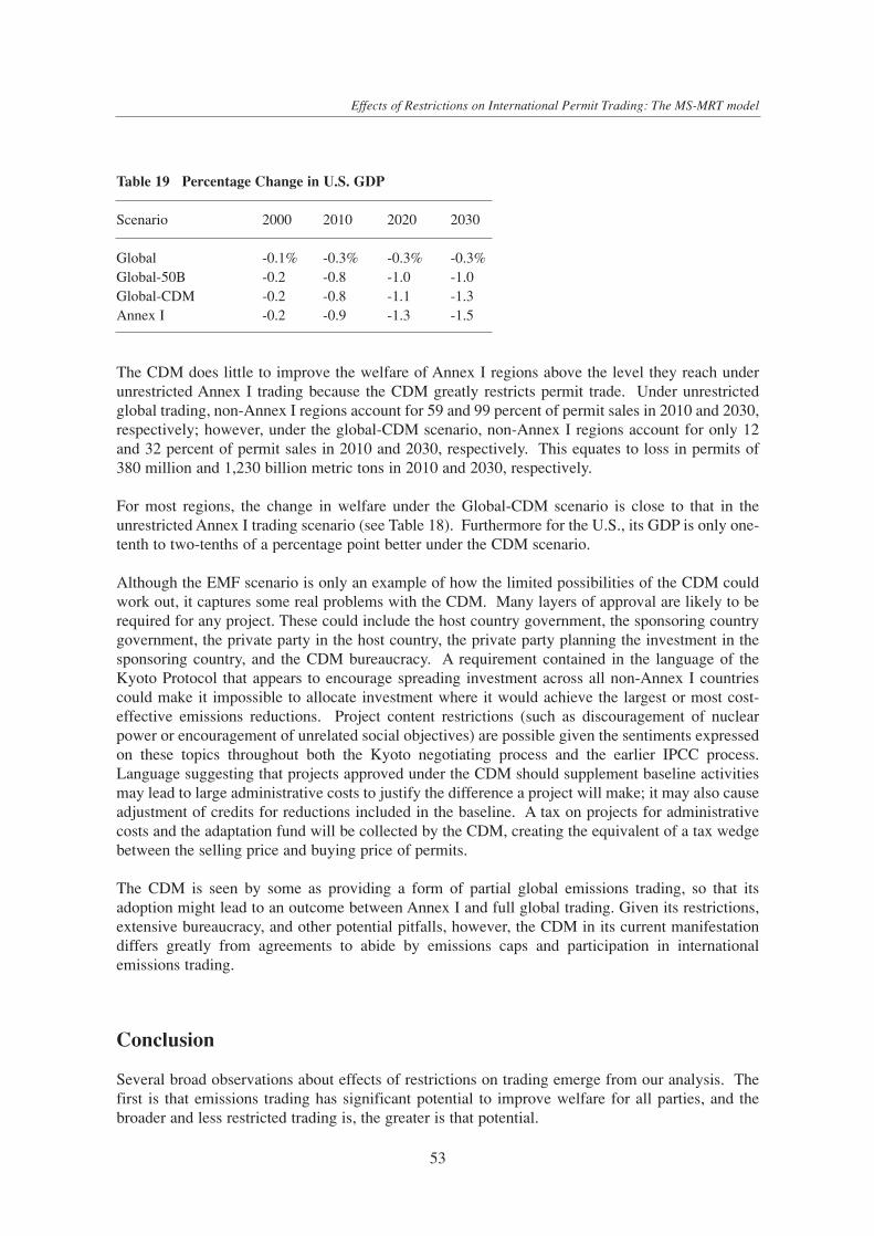
The CDM does little to improve the welfare of Annex I regions above the level they reach underunrestricted Annex I trading because the CDM greatly restricts permit trade. Under unrestrictedglobal trading, non-Annex I regions account for 59 and 99 percent of permit sales in 2010 and 2030,respectively; however, under the global-CDM scenario, non-Annex I regions account for only 12and 32 percent of permit sales in 2010 and 2030, respectively. This equates to loss in permits of380 million and 1,230 billion metric tons in 2010 and 2030, respectively.
For most regions, the change in welfare under the Global-CDM scenario is close to that in theunrestricted Annex I trading scenario (see Table 18). Furthermore for the U.S., its GDP is only one-tenth to two-tenths of a percentage point better under the CDM scenario.
Although the EMF scenario is only an example of how the limited possibilities of the CDM couldwork out, it captures some real problems with the CDM. Many layers of approval are likely to berequired for any project. These could include the host country government, the sponsoring countrygovernment, the private party in the host country, the private party planning the investment in thesponsoring country, and the CDM bureaucracy. A requirement contained in the language of theKyoto Protocol that appears to encourage spreading investment across all non-Annex I countriescould make it impossible to allocate investment where it would achieve the largest or most cost-effective emissions reductions. Project content restrictions (such as discouragement of nuclearpower or encouragement of unrelated social objectives) are possible given the sentiments expressedon these topics throughout both the Kyoto negotiating process and the earlier IPCC process.Language suggesting that projects approved under the CDM should supplement baseline activitiesmay lead to large administrative costs to justify the difference a project will make; it may also causeadjustment of credits for reductions included in the baseline. A tax on projects for administrativecosts and the adaptation fund will be collected by the CDM, creating the equivalent of a tax wedgebetween the selling price and buying price of permits.
The CDM is seen by some as providing a form of partial global emissions trading, so that itsadoption might lead to an outcome between Annex I and full global trading. Given its restrictions,extensive bureaucracy, and other potential pitfalls, however, the CDM in its current manifestationdiffers greatly from agreements to abide by emissions caps and participation in internationalemissions trading.
Conclusion
Several broad observations about effects of restrictions on trading emerge from our analysis. Thefirst is that emissions trading has significant potential to improve welfare for all parties, and thebroader and less restricted trading is, the greater is that potential.
53
Effects of Restrictions on International Permit Trading: The MS-MRT model
Table 19 Percentage Change in U.S. GDP
Scenario 2000 2010 2020 2030
Global -0.1% -0.3% -0.3% -0.3%Global-50B -0.2 -0.8 -1.0 -1.0Global-CDM -0.2 -0.8 -1.1 -1.3Annex I -0.2 -0.9 -1.3 -1.5

The second is that developing countries will not escape costs, even if they do not participate inemissions trading because changes in the terms of trade shift some of the cost of Annex I-onlyemissions reductions onto developing countries. In general, less restricted trading has the potentialto benefit developing countries. In our results, developing countries are potentially better off underglobal trading than under no trading and in general they are better off under Annex I trading thanunder no trading. Achieving this potential will require delicate negotiations about the initialallocation of permits – the cap assigned to developing countries.
In general, restricting emissions trade reduces global welfare, but within that global total somecountries gain and some lose from restrictions. In many cases, the countries advocating restrictionsare those most harmed by them. How impacts are distributed depends strongly on assumptionsabout baselines and elasticities, suggesting that distributional issues are likely to remain contentious.
Exercise of market power is clearly possible under policies like Annex I trading that create marketswith a single seller, but our estimates suggest that it is easy to choose policies that are worse thanthe exercise of market power. For example, prohibiting sales of hot air would restrict sales and raisepermit prices higher than it would ever be in the interest of Russia acting as a monopolist. Choosingnot to interfere with the possibility of market power may be better for the world than capping thesales of permits.
In terms of restrictions on trading that includes developing countries, CDM would provide smallbenefits relative to global trading, if its operations are subject to constraints now under discussion.Limits on purchases of permits by Annex 1 countries would largely eliminate benefits the U.S. couldachieve by extending permit trading to developing countries.
Finally, Annex 1 trading does not significantly reduce leakage. Full global trading is required toprevent increases in emissions in non-participating countries.
54
Paul M. Bernstein, W. David Montgomery, Thomas F. Rutherford, Gui-Fang Yang

References
Armington, Paul, “A Theory of Demand for ProductsDistinguished by Place of Production,” IMF Staff Papers16 (1969), 159-178.
Babiker, Mustafa H., and Thomas F. Rutherford,“GTAPinGAMS: Tools for Energy-EconomyModeling,” Working Paper, University of ColoradoDepartment of Economics, 1998.
Babiker, Mustafa H., Keith E. Maskus, and Thomas F.Rutherford, “Carbon Taxes and the Global TradingSystem,” Working Paper, University of ColoradoDepartment of Economics, 1997.
Bernstein, Paul M., W. David Montgomery, and Thomas F.Rutherford, “Trade Impacts of Climate Policy: The MS-MRT Model,” in review, Energy and ResourceEconomics, 1998.
Edmonds, J.A., H.M. Pitcher, D. Barns, R. Baron, andM.A. Wise, “Modelling future greenhouse gasemissions: the second generation model description,” inModelling Global Change, Lawrence R. Klein and Fu-Chen Lo, Eds. (Tokyo, Japan: United Nations UniversityPress, 1992), pp. 295-340.
Edmonds, J.A., et al., “Return to 1990: The Cost ofMitigating United States Carbon Emissions in the Post-2000 Period,” October 1997
Hertel, Thomas W. (ed.), Global Trade Analysis: Modelingand Applications (Cambridge, UK: CambridgeUniversity Press, 1997).
Manne, Alan S. and Richard Richels, Buying GreenhouseInsurance: The Economic Costs of CO2 Emission Limits(Cambridge, MA: MIT Press, 1990).
Manne, Alan S., and Thomas F. Rutherford, “InternationalTrade, Capital Flows, and Sectoral Analysis: AFormulation and Solution of Intertemporal Equilibrium Models,” in New Directions in ComputationalEconomics, William W. Cooper and AndrewB.Whinston, eds. (1994), pp. 191-205.
Markusen, J.R., and J.R. Melvin, “The Theory ofInternational Trade and Its Canadian Applications,”(Butterworths, 1984).
McKibbin, Warwick J. and Peter J. Wilcoxen, “TheTheoretical and Empirical Structure of the G-CubedModel,” Working Paper, The Brookings Institution,1995.
Pepper, William, Jane Leggett, Rob Swart, John Watson,Jae Edmonds, and Irving Mintzer, “Emission Scenariosfor the IPCC: An Update — Assumptions,Methodology, and Results,” prepared for theIntergovernmental Panel on Climate Change WorkingGroup, May 1992.
President’s Council of Economic Advisors, “The KyotoProtocol and the President’s Policies to Address ClimateChange: Administration Economic Analysis,”Washington, DC, July 1998.
Rutherford, Thomas F., “GTAPinGAMS: The Dataset andStatic Model,” Working Paper, University of ColoradoDepartment of Economics, 1998.
Rutherford, Thomas F., Morten Lau, and Andreas Pahlke,“A Primer in Dynamic General Equilibrium Analysis,”Working Paper, University of Colorado Department ofEconomics, 1998.
U.S. Department of Energy, Energy InformationAdministration, Annual Energy Outlook, 1998,DOE/EIA-0383(98), Washington, DC, 1997.
Varian, Microeconomic Analysis, Third Edition, New York,1992, pp. 160-171.
55
Effects of Restrictions on International Permit Trading: The MS-MRT model

56

Discussion
Snorre Kverndokk
The paper by Bernstein et al. (1999) presents economic impacts of the Kyoto agreement using adynamic general equilibrium model (MS-MRT model). The model is a multi-sector, multi-regiontrade model, and simulations are run for the period 2000-2030. The focus of the model is the effectsof emission permit trading, and three different regimes are studied. In the first regime, there is notrading, while trading only among Annex 1 countries is allowed in the second regime. Finally, in thethird regime, full global trading is allowed. Impacts on such variables as economic welfare,international trade and investments across regions, the spillover effects of carbon emission limits inAnnex 1 countries on non-Annex 1 countries, carbon leakage, changes in terms of trade and industryoutput are studied under the different regimes. The results are well documented, and sensitivityanalyses are made to test the robustness of the results.
The paper analyses a very important question, namely the impacts of the Kyoto agreement. This isan important task as it provides useful background information for the forthcoming negotiations,both for the final framing of the Kyoto agreement, and also for the discussions of an agreement afterthe Kyoto period of 2008-2012. However, one question the reader asks himself when studying amodel simulation of the Kyoto agreement is what does this paper tell me that I have not readsomewhere else? What is new in this study, and does the model provide some new insight?Unfortunately the authors do not help us very much in answering these questions. They do not referto similar analyses, or compare their results. Over the last year or so, several modellers around theworld have made simulations of the Kyoto agreement on their national, regional or global models,and some of these papers will be published in a forthcoming number of the Energy Journal. WhatI think is the main contribution of this study is that the model is both dynamic, and also rich insectoral and regional specification. Besides this, trade with several goods is modelled. Thus, themodel covers several important aspects at the same time, maybe more than other global models, andI therefore think that it makes an important contribution to study the impacts of the Kyotoagreement. In the following, I will not comment so much on the specific results, but focus onsubjects that I feel is important, is a bit unclear or maybe not satisfactory studied by the analysis.
One reason to have a dynamic model is the fossil fuel markets. The aspects of non-renewable goodsrequire a dynamic model. This is especially important when analysing climate treaties, as about 75per cent of CO2 emissions are due to the combustion of fossil fuels. However, fossil fuels are notfully modelled as non-renewable resources as the depletion effects are ignored. This leaves out thequestion of the rational distribution of production over time. Another important question is strategictype of the markets. As far as I understand, perfect competition is assumed in all markets, also theoil market. But imperfect competition is a characteristic of the oil market. As documented in Berget al. (1997), whether there is perfect or imperfect competition in the oil market have large impactson the effects of a climate treaty, for instance the effects on the oil price. With imperfect competition(OPEC as a cartel), the producer price of oil is not much affected the first years after an agreementhas come into force, and the carbon leakage may therefore also be minor. The significant leakage inBernstein et al. in the scenario with no international permit trading may, therefore, partly beexplained by perfect competition in the oil market.
57
Effects of Restrictions on International Permit Trading: The MS-MRT model

Even if the model has a high number of sectors, one important sector is not modelled, namelyforestry. Land use changes are included in the Kyoto protocol, which makes this sector interestingin an analysis like this. A national CGE model where emissions from the use of timber and carbonaccumulation in the forest are taken into account, thus calculating net emissions, is Pohjola (1999).If net emissions are taxed, Pohjola (1999) finds that the carbon tax needed to reduce net emissionsby the same amount as emissions from fossil fuels is significantly lower.
International trade is an important aspect of the model. However, the paper could focus more onhow international trade can reduce economic costs of a climate treaty, especially when permittrading is not allowed. One example is electricity trade. Electricity is produced using a number ofproduction technologies, and the amount of carbon emissions per unit of electricity varies a lotbetween the technologies. One example is electricity trade in Scandinavia, where electricity inNorway is based on hydropower, while it is mainly based on coal in Denmark. Norway can increaseits production of hydropower without increasing CO2 emissions. If Denmark imports electricityfrom Norway, Danish emissions will be reduced. Thus, as demonstrated in Hauch (1999), if nationalemission targets are imposed, Danish emissions can be reduced at a lower cost if electricity is tradedcompared to a situation with no trade. Electricity trade can actually work as a substitute to permittrading and equalise marginal abatement costs. Natural gas is another good that may help equalisingmarginal abatement cost via international trade.
The model includes a backstop technology, which sets an upper limit on the price of fossil fuels.That the backstop technology is important for future carbon emissions is demonstrated in, e.g.,Chakravorty et al. (1997). As far as I understand, the technological change in the backstoptechnology is exogenous in the model. However, there is a possibility that a carbon treaty speeds upresearch and development for alternative energy resources, and therefore, reduces the costs of futureabatement. This is an important subject, and I hope to take a further look at this issue in the nearfuture.
The paper calculates the welfare impacts under alternative trading arrangements. The welfareconcept in this analysis does not include environmental impacts. Personally, I do not like to use theword welfare when environmental impacts are not included, as the main reason for reducingemissions is the well being or welfare of people. Environmental impacts can include both primaryand secondary benefits. As demonstrated by several CGE models, the secondary benefits fromgreenhouse gas abatement may actually outweigh the abatement costs, see, e.g., Ekins (1996). Oneinteresting aspect is the feedback from the environment to the economy. A few CGE models haveincorporated this. One example is Glomsrød et al. (1998) that studies the impacts of traffic injurieson labour supply and public health expenditures in a CGE model for Norway. A carbon tax reducesthe fossil fuel use and thus the traffic volume, leading to fewer accidents and increased laboursupply.
One of the permit trading regimes in the paper is global permit trading. However, it is a bit hard tosee from the paper how this actually is specified, and also how the emission targets are specifiedafter 2010. It would help the reader if graphs showing carbon emissions were included. How thisregime is specified is important. One of the flexible mechanisms in the Kyoto protocol is the CleanDevelopment Mechanism (CDM). This may be interpreted as a kind of global permit emissiontrading. However, this mechanism may lead to higher global emissions as it gives the non-Annex 1countries an incentive to delay investments as Annex 1 countries may pay for the investments in afuture period. One of the conclusions in the paper is that global permit trading is worse for Chinaand India than no permit trading, which may explain their attitudes towards permit trading.However, this is very dependent on how the emission permits are distributed after the Kyoto period
58
Snorre Kverndokk
2008-12, and this should, therefore, be made clearer in the paper. As demonstrated in, e.g.,Kverndokk (1993), different permit allocation rules give very different transfers between countries,and allocation rules may be constructed that actually benefit countries like India and China (e.g., apopulation rule). Therefore, I think a discussion on emission targets after the model period of 2010is important, and different regional targets could also be analysed.
I have made several comments on how the analysis could be broadened. However, this does notmean that I do not find the paper interesting, or that I think a general equilibrium analysis shouldinclude all this aspects. Anyway, I think that the paper may be improved if some of the aspects arementioned and relevant comparisons are made.
59
Effects of Restrictions on International Permit Trading: The MS-MRT model
References
Berg, E., S. Kverndokk, and K. E. Rosendahl, 1997:Market power, international CO2 taxation and petroleumwealth. The Energy Journal, 18(4), 33-71.
Bernstein, P. M., W. D. Montgomery, and T. F. Rutherford,1999: Global Impacts of the Kyoto Agreement: Resultsfrom the MS-MRT Model. Paper presented at the IPCCWorking Group III Expert Meeting, May 27-28, TheHague, The Netherlands.
Chakravorty, U., J. Roumasset, and K. Tse, 1997:Endogenous substitution among energy resources andglobal warming. Journal of Political Economy, 105(6),1201-1234.
Ekins, P., 1996: How large a carbon tax is justified by thesecondary benefits of CO2 abatement? Resource andEnergy Economics, 18(2), 161-187.
Glomsrød, S., R. Nesbakken, and M. Aaserud, 1998:Modelling impacts of traffic injuries on labour supplyand public health expenditures. In Social Costs of AirPollution and Fossil Fuel Use – A MacroeconomicApproach. K. E. Rosendahl, (ed.), Social and EconomicStudies 99, Statistics Norway.
Hauch, J., 1999: Elephant – A Simulation Model forEnvironmental Regulation at Nordic Energy Markets.Ph.D thesis, Danish Economic Council, Copenhagen.
Kverndokk, S., 1993: Global CO2 Agreements: A CostEffective Approach. The Energy Journal, 14(2), 91-112.
Pohjola, J., 1999: Economywide Effects of Reducing CO2Emissions: A Comparison between Net and GrossEmissions. Journal of Forest Economics, 5(1), 139-168.

60

Emissions Trading, Capital Flows and the Kyoto Protocol
Warwick J. McKibbin, Martin T. Ross, Robert Shackleton, and Peter J. Wilcoxen
1 Introduction
As part of an effort to reduce global emissions of greenhouse gases (GHGs) that are expected tocontribute to a significant warming of the earth’s climate, the Kyoto Protocol to the United NationsFramework Convention on Climate Change, signed in Kyoto in December 1997, includes bindingGHG emissions targets for the world’s industrial economies (“Annex I” countries) for the period2008-2012. The Protocol also provides for international trading of emission allowances among thecountries that accept binding targets, in recognition of the theoretical efficiency benefits of allowingemission reductions to be obtained at least cost. In addition, the Protocol provides for a CleanDevelopment Mechanism, under which agents from industrial countries can earn emission creditsfor certified reductions from investments in “clean development” projects in developing countriesthat have not taken on binding targets.
In this paper we present estimates of the potential economic effects of the Kyoto Protocol, using theG-Cubed multi-region, multi-sector intertemporal general equilibrium model of the worldeconomy.1 We examine and compare four potential implementations of the Protocol involvingvarying degrees of international permit trading, focusing particularly on short term dynamics and onthe effects of the policies on output, exchange rates and international flows of goods and financialcapital. We present calculations of some of the gains from allowing international permit trading, andexamine the sensitivity of the results to changes in the most important assumptions.
2 Model Structure
In this section we give a necessarily brief overview of the key features of the model underlying thisstudy, that are important in understanding the results. For a more complete coverage of the model,please see McKibbin and Wilcoxen (1995b).2
The G-Cubed model consists of a set of eight regional general equilibrium models linked byconsistent international flows of goods and assets. We assume that each region consists of arepresentative household, a government sector, a financial sector, twelve industries, and two sectorsproducing capital goods for the producing industries and households, respectively. The regions and
61
Emissions Trading, Capital Flows and the Kyoto Protocol
1 G-Cubed stands for “Global General Equilibrium Growth Model.” An earlier draft of this paper used version 31 of the model. Thisdraft uses version 39, which includes significant data updates and has emission coefficients on gas and oil separately rather than on thecrude oil and gas extraction sector
2 This and other papers describing the model are available at http:\www.msgpl.com.au.
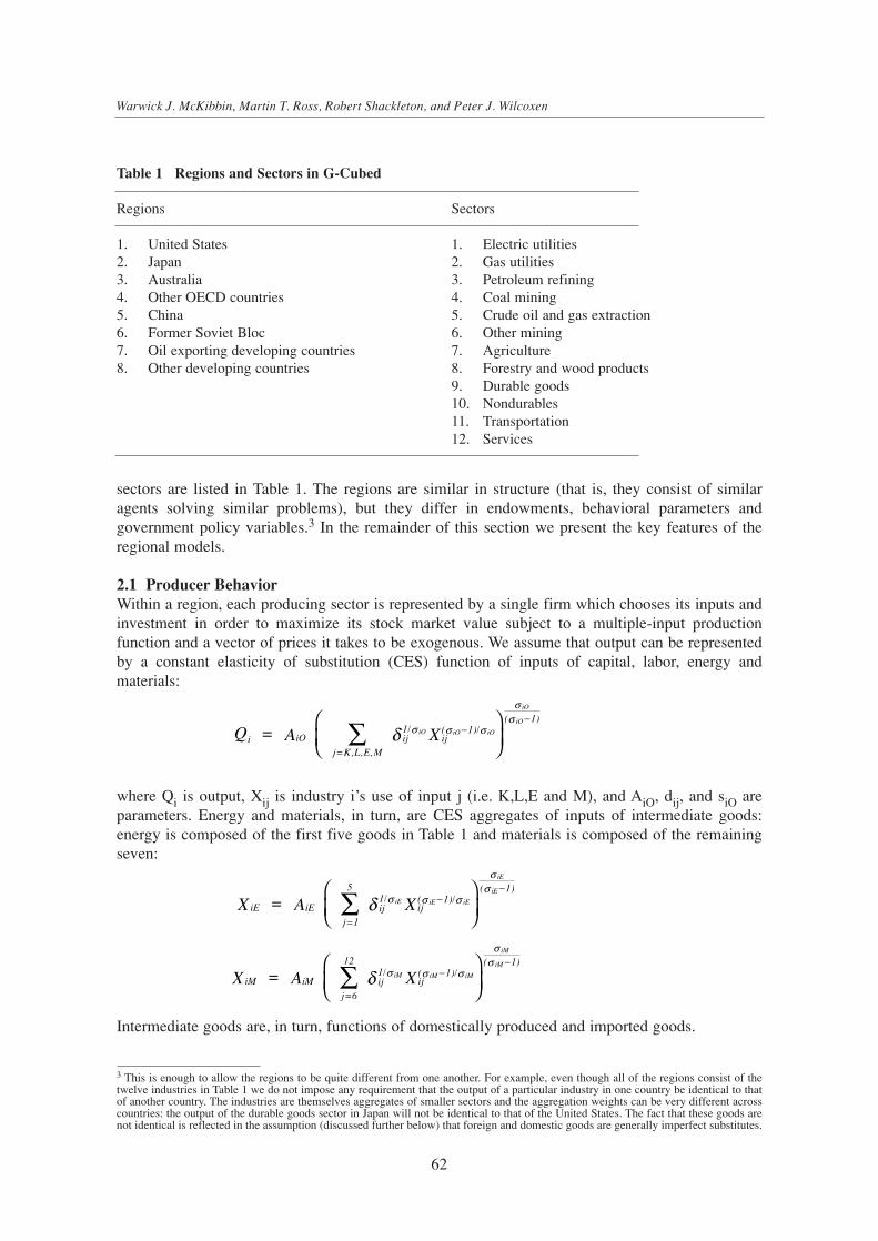
sectors are listed in Table 1. The regions are similar in structure (that is, they consist of similaragents solving similar problems), but they differ in endowments, behavioral parameters andgovernment policy variables.3 In the remainder of this section we present the key features of theregional models.
2.1 Producer BehaviorWithin a region, each producing sector is represented by a single firm which chooses its inputs andinvestment in order to maximize its stock market value subject to a multiple-input productionfunction and a vector of prices it takes to be exogenous. We assume that output can be representedby a constant elasticity of substitution (CES) function of inputs of capital, labor, energy andmaterials:
where Qi is output, Xij is industry i’s use of input j (i.e. K,L,E and M), and AiO, dij, and siO areparameters. Energy and materials, in turn, are CES aggregates of inputs of intermediate goods:energy is composed of the first five goods in Table 1 and materials is composed of the remainingseven:
Intermediate goods are, in turn, functions of domestically produced and imported goods.
iM iM
( 1)
j=6
12
ij1/
ij( 1)/X = A X
iM
iM
iM iM iM
σσ
σ σ σδ−
−∑
iE iE
( 1)
j=1
5
ij1/
ij( 1)/X = A X
iE
iE
iE iE iE
σσ
σ σ σδ−
−∑
i iO
( 1)
j=K,L,E,M
ij1/
ij( 1)/Q = A X
iO
iO
iO iO iO
σσ
σ σ σδ−
−∑
Warwick J. McKibbin, Martin T. Ross, Robert Shackleton, and Peter J. Wilcoxen
62
Table 1 Regions and Sectors in G-Cubed
Regions Sectors
1. United States 1. Electric utilities2. Japan 2. Gas utilities3. Australia 3. Petroleum refining4. Other OECD countries 4. Coal mining5. China 5. Crude oil and gas extraction6. Former Soviet Bloc 6. Other mining7. Oil exporting developing countries 7. Agriculture8. Other developing countries 8. Forestry and wood products
9. Durable goods10. Nondurables11. Transportation12. Services
3 This is enough to allow the regions to be quite different from one another. For example, even though all of the regions consist of thetwelve industries in Table 1 we do not impose any requirement that the output of a particular industry in one country be identical to thatof another country. The industries are themselves aggregates of smaller sectors and the aggregation weights can be very different acrosscountries: the output of the durable goods sector in Japan will not be identical to that of the United States. The fact that these goods arenot identical is reflected in the assumption (discussed further below) that foreign and domestic goods are generally imperfect substitutes.

We use a nested system of CES equations rather than a more flexible functional form because datalimitations make even the CES model a challenge to estimate. In principle, to estimate a moreflexible specification we would need time-series price and quantity data for 14 inputs (twelve goodsplus capital and labor) in each of 96 industries (12 industries in 8 regions). Unfortunately, nocountry collects annual data on intermediate inputs, and most developing countries collect almostno industry data at all.
The scarcity of input-output data requires us to restrict the model further by imposing theassumption that each industry has the same energy, materials and KLEM substitution elasticities nomatter where it is located (although the elasticities differ across industries).4 However, even thoughthe substitution elasticities are identical across countries, the overall production models differbecause the CES input weights are taken from the latest available input-output data for each countryor region.5 Thus, the durable goods sectors in the United States and Japan, for example, haveidentical substitution elasticities but different sets of input weights. The consequence of this is thatthe cost shares of inputs to a given industry are based on data for the country in which the industryoperates, but the industry’s response to a given percentage increase in an input price is identicalacross countries. Taken together, these assumptions are equivalent to assuming that all regions shareproduction methods that differ in first-order properties but have identical second-ordercharacteristics. This approach is intermediate between one extreme of assuming that the regionsshare common technologies and the other extreme of allowing the technologies to differ acrossregions in arbitrary ways.
The regions also differ in their endowments of primary factors, their government policies, andpatterns of final demands, so although they share some common parameters they are not simplereplicas of one another.
To estimate the elasticities we have constructed time-series data on prices, industry inputs, outputsand value-added for the country for which we were able to obtain the longest series of input-outputtables: the United States. The following is a sketch of the approach; complete details are containedin McKibbin and Wilcoxen (forthcoming).
We began with the benchmark input-output transactions tables produced by the Bureau of EconomicAnalysis (BEA) for years 1958, 1963, 1967, 1972, 1977 and 1982.6 The conventions used by theBEA have changed over time, so the raw tables are not completely comparable. We transformed thetables to make them consistent and aggregated them to twelve sectors. We then shifted consumerdurables out of final consumption and into fixed investment.7 We also increased the capital serviceselement of final consumption to account for imputed service flows from durables and owner-occupied housing. Finally, we used a data set constructed by Dale Jorgenson and his colleagues todecompose the value-added rows of the tables,8and a data set produced by the Office ofEmployment Projections at the Bureau of Labor Statistics to provide product prices.
63
Emissions Trading, Capital Flows and the Kyoto Protocol
4 This assumption is consistent with the available econometric evidence (see for example Kim and Lau, 1994).
5 Input-output tables were not available for the regions in the model larger than individual countries. The input weights for those regionswere based on data for the United States.
6 A benchmark table also exists for 1947 but it has inadequate final demand detail for our purposes. Subsequent to our estimation worka 1987 table has become available.
7 The National Income and Product Accounts (and the benchmark input-output tables as well) treat purchases of consumer durables asconsumption rather than investment.
8 This data set is the work of several people over many years. In addition to Dale Jorgenson, some of the contributors were LauChristiansen, Barbara Fraumeni, Mun Sing Ho and Dae Keun Park. The original source of data is the Fourteen Components of IncomeTape produced by the Bureau of Economic Analysis. See Ho (1989) for more information.
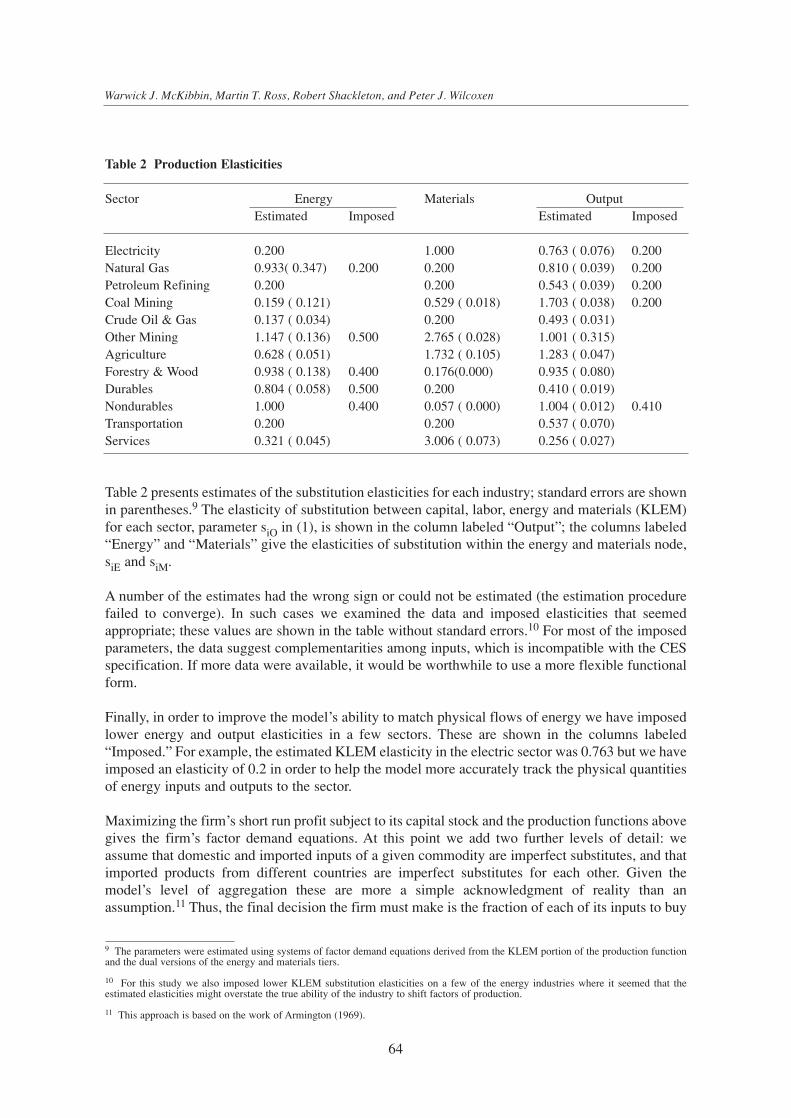
Table 2 presents estimates of the substitution elasticities for each industry; standard errors are shownin parentheses.9 The elasticity of substitution between capital, labor, energy and materials (KLEM)for each sector, parameter siO in (1), is shown in the column labeled “Output”; the columns labeled“Energy” and “Materials” give the elasticities of substitution within the energy and materials node,siE and siM.
A number of the estimates had the wrong sign or could not be estimated (the estimation procedurefailed to converge). In such cases we examined the data and imposed elasticities that seemedappropriate; these values are shown in the table without standard errors.10 For most of the imposedparameters, the data suggest complementarities among inputs, which is incompatible with the CESspecification. If more data were available, it would be worthwhile to use a more flexible functionalform.
Finally, in order to improve the model’s ability to match physical flows of energy we have imposedlower energy and output elasticities in a few sectors. These are shown in the columns labeled“Imposed.” For example, the estimated KLEM elasticity in the electric sector was 0.763 but we haveimposed an elasticity of 0.2 in order to help the model more accurately track the physical quantitiesof energy inputs and outputs to the sector.
Maximizing the firm’s short run profit subject to its capital stock and the production functions abovegives the firm’s factor demand equations. At this point we add two further levels of detail: weassume that domestic and imported inputs of a given commodity are imperfect substitutes, and thatimported products from different countries are imperfect substitutes for each other. Given themodel’s level of aggregation these are more a simple acknowledgment of reality than anassumption.11 Thus, the final decision the firm must make is the fraction of each of its inputs to buy
Warwick J. McKibbin, Martin T. Ross, Robert Shackleton, and Peter J. Wilcoxen
64
Table 2 Production Elasticities
Sector Energy Materials OutputEstimated Imposed Estimated Imposed
Electricity 0.200 1.000 0.763 ( 0.076) 0.200Natural Gas 0.933( 0.347) 0.200 0.200 0.810 ( 0.039) 0.200Petroleum Refining 0.200 0.200 0.543 ( 0.039) 0.200Coal Mining 0.159 ( 0.121) 0.529 ( 0.018) 1.703 ( 0.038) 0.200Crude Oil & Gas 0.137 ( 0.034) 0.200 0.493 ( 0.031)Other Mining 1.147 ( 0.136) 0.500 2.765 ( 0.028) 1.001 ( 0.315)Agriculture 0.628 ( 0.051) 1.732 ( 0.105) 1.283 ( 0.047)Forestry & Wood 0.938 ( 0.138) 0.400 0.176(0.000) 0.935 ( 0.080)Durables 0.804 ( 0.058) 0.500 0.200 0.410 ( 0.019)Nondurables 1.000 0.400 0.057 ( 0.000) 1.004 ( 0.012) 0.410Transportation 0.200 0.200 0.537 ( 0.070)Services 0.321 ( 0.045) 3.006 ( 0.073) 0.256 ( 0.027)
9 The parameters were estimated using systems of factor demand equations derived from the KLEM portion of the production functionand the dual versions of the energy and materials tiers.
10 For this study we also imposed lower KLEM substitution elasticities on a few of the energy industries where it seemed that theestimated elasticities might overstate the true ability of the industry to shift factors of production.
11 This approach is based on the work of Armington (1969).
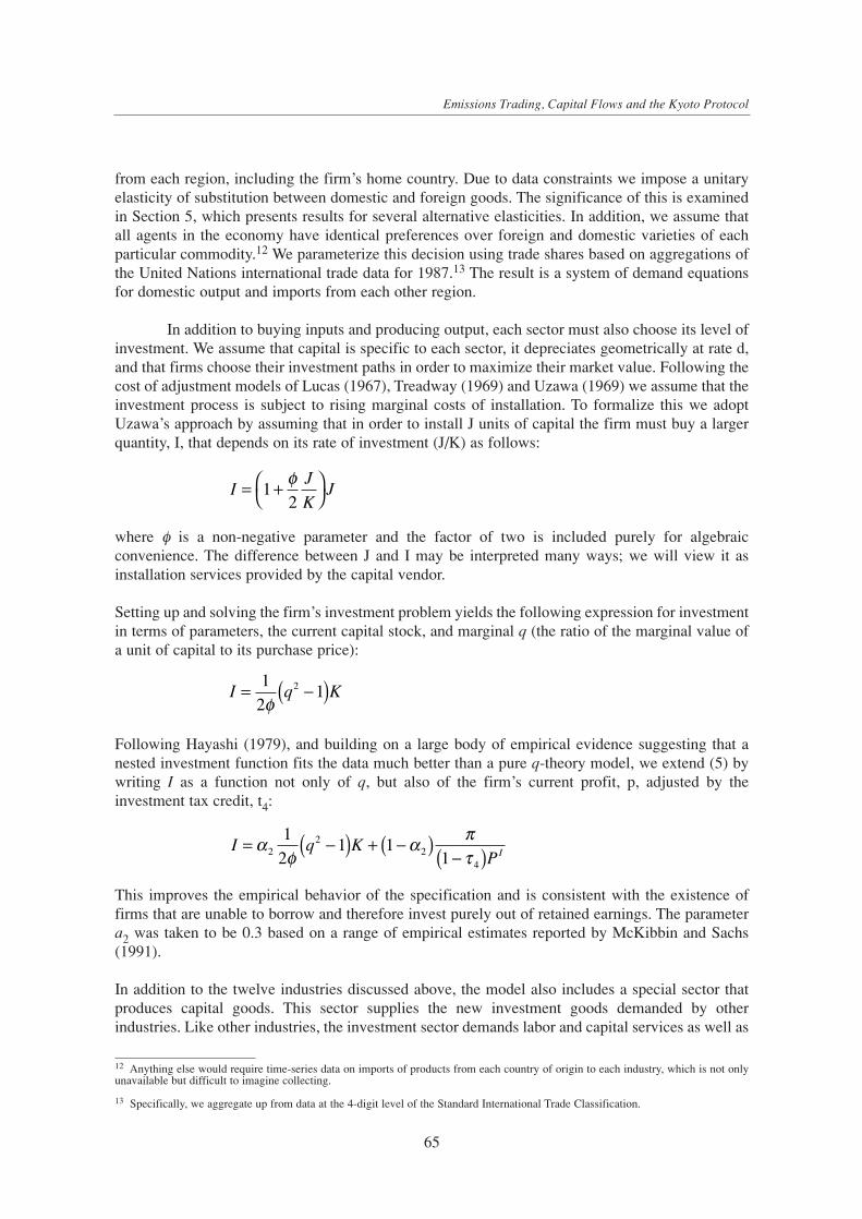
from each region, including the firm’s home country. Due to data constraints we impose a unitaryelasticity of substitution between domestic and foreign goods. The significance of this is examinedin Section 5, which presents results for several alternative elasticities. In addition, we assume thatall agents in the economy have identical preferences over foreign and domestic varieties of eachparticular commodity.12 We parameterize this decision using trade shares based on aggregations ofthe United Nations international trade data for 1987.13 The result is a system of demand equationsfor domestic output and imports from each other region.
In addition to buying inputs and producing output, each sector must also choose its level ofinvestment. We assume that capital is specific to each sector, it depreciates geometrically at rate d,and that firms choose their investment paths in order to maximize their market value. Following thecost of adjustment models of Lucas (1967), Treadway (1969) and Uzawa (1969) we assume that theinvestment process is subject to rising marginal costs of installation. To formalize this we adoptUzawa’s approach by assuming that in order to install J units of capital the firm must buy a largerquantity, I, that depends on its rate of investment (J/K) as follows:
where φ is a non-negative parameter and the factor of two is included purely for algebraicconvenience. The difference between J and I may be interpreted many ways; we will view it asinstallation services provided by the capital vendor.
Setting up and solving the firm’s investment problem yields the following expression for investmentin terms of parameters, the current capital stock, and marginal q (the ratio of the marginal value ofa unit of capital to its purchase price):
Following Hayashi (1979), and building on a large body of empirical evidence suggesting that anested investment function fits the data much better than a pure q-theory model, we extend (5) bywriting I as a function not only of q, but also of the firm’s current profit, p, adjusted by theinvestment tax credit, t4:
This improves the empirical behavior of the specification and is consistent with the existence offirms that are unable to borrow and therefore invest purely out of retained earnings. The parametera2 was taken to be 0.3 based on a range of empirical estimates reported by McKibbin and Sachs(1991).
In addition to the twelve industries discussed above, the model also includes a special sector thatproduces capital goods. This sector supplies the new investment goods demanded by otherindustries. Like other industries, the investment sector demands labor and capital services as well as
I q KPI= −( ) + −( )
−( )αφ
α πτ2
22
4
12
1 11
I q K= −( )12
12
φ
IJ
KJ= +
1
2φ
65
Emissions Trading, Capital Flows and the Kyoto Protocol
12 Anything else would require time-series data on imports of products from each country of origin to each industry, which is not onlyunavailable but difficult to imagine collecting.
13 Specifically, we aggregate up from data at the 4-digit level of the Standard International Trade Classification.

intermediate inputs. We represent its behavior using a nested CES production function with thesame structure as that used for the other sectors, and we estimate the parameters using price andquantity data for the final demand column for investment. As before, we use U.S. data to estimatethe substitution elasticities and country or region data to determine the share parameters.
2.2 HouseholdsHouseholds consume goods and services in every period and also demand labor and capital services.Household capital services consist of the service flows of consumer durables plus residentialhousing. Households receive income by providing labor services to firms and the government, andby holding financial assets. In addition, they receive imputed income from ownership of durablesand housing, and they also may receive transfers from their region’s government.
Within each region we assume household behavior can be modeled by a representative agent withan intertemporal utility function of the form:
\where C(s) is the household’s aggregate consumption of goods at time s, G(s) is governmentconsumption, which we take to be a measure of public goods supply, and q is the rate of timepreference and is equal to 2.5 percent.14 The household maximizes its utility subject to the constraintthat the present value of consumption be equal to human wealth plus initial financial assets. Humanwealth, H, is the present value of the future stream of after-tax labor income and transfer paymentsreceived by households. Financial wealth, F, is the sum of real money balances, real governmentbonds in the hands of the public (Ricardian neutrality does not hold in this model because someconsumers are liquidity-constrained; more on this below), net holdings of claims against foreignresidents and the value of capital in each sector. A full derivation can be found in McKibbin andSachs (1991) and McKibbin and Wilcoxen (forthcoming).
Under this specification, it is easy to show that the desired value of each period’s consumption isequal to the product of the time preference rate and household wealth:
There has, however, been considerable debate about whether the actual behavior of aggregateconsumption is consistent with the permanent income model.15 Based on a wide range of empiricalevidence in the macroeconomics literature (see Campbell and Mankiw, 1990), we impose that onlya fraction b of all consumers choose their consumption to satisfy (8) and that the remainder consumebased entirely on current after-tax income. We have deliberately chosen to depart from thetheoretical elegance of (8) because we are evaluating real-world policy and it is absolutely clearfrom empirical data that (8) alone is not a satisfactory model of aggregate consumption. This is animportant difference between our approach and many of the other models used to study climatechange policy, where theoretical elegance has often been given greater importance than realism.
)( H+F = CPC θ
t
t
- s-tU = C s + G s e ds∞
∫ (ln ( ) ln ( )) ( )θ
Warwick J. McKibbin, Martin T. Ross, Robert Shackleton, and Peter J. Wilcoxen
66
14 This specification imposes the restriction that household decisions on the allocations of expenditure among different goods at differentpoints in time be separable. Also, since utility is additive in the logs of private and government consumption, changes in governmentconsumption will have no effect on private consumption decisions.
15 Some of the key papers in this debate are Hall (1978), Flavin (1981), Hayashi (1982), and Campbell and Mankiw (1990).

Whenever we have had to choose between theoretical elegance and empirical relevance, we havechosen the latter.16
The empirical finding that pure permanent income models such as (8) are rejected by the data whilenested functions that include a large weight on current income fit much better could be interpretedin various ways, including the presence of liquidity-constrained households or households withmyopic expectations. For the purposes of this paper we will not adopt any particular explanation butsimply take b to be an exogenous constant.17 This produces the final consumption function shownbelow:
where g is the marginal propensity to consume for the households consuming out of current income.Following McKibbin and Sachs (1991) we take b to be 0.3 in all regions.18
Within each period, the household allocates expenditure among goods and services in order tomaximize C(s), its intratemporal utility index. In this version of the model we assume that C(s) maybe represented by a nested CES function. At the top tier, consumption is composed of inputs ofcapital services, labor, energy and materials. Energy and materials, in turn, are CES aggregates ofinputs of individual goods.19 The elasticities of substitution at the energy and materials tiers wereestimated to be 0.8 and 1.0, respectively. In this version of the model the top tier elasticity has beenimposed to be unity.
Finally, the supply of household capital services is determined by consumers themselves who investin household capital. We assume households choose the level of investment to maximize the presentvalue of future service flows (taken to be proportional to the household capital stock), and thatinvestment in household capital is subject to adjustment costs. In other words, the householdinvestment decision is symmetrical with that of the firms.
2.3 Labor Market EquilibriumWe assume that labor is perfectly mobile among sectors within each region but is immobile betweenregions. Thus, within each region wages will be equal across sectors. The nominal wage is assumedto adjust slowly according to an overlapping contracts model (adjusted for different labor marketinstitutional structures in different economies) where nominal wages are set based on current andexpected inflation and on economy-wide labor demand relative to labor supply. In the long run laborsupply, which is specified in terms of labor efficiency units, is given by the exogenous rate ofpopulation growth, but in the short run the hours worked can fluctuate depending on the demand forlabor. For a given nominal wage, the demand for labor will determine short-run unemployment.
Relative to other general equilibrium models, this specification is unusual in allowing forinvoluntary unemployment. We adopt this approach because we are particularly interested in the
INC + H+F= CP ttC γββθ )1()( −
67
Emissions Trading, Capital Flows and the Kyoto Protocol
16 One complication of introducing a nested specification for consumption is that traditional welfare evaluations are difficult. However,we view it as far more important to take empirical facts into account than for it to be easy to calculate equivalent variations.
17 One side effect of this specification is that it will prevent us from using equivalent variation or other welfare measures derived fromthe expenditure function. Since the behavior of some of the households is implicitly inconsistent with the previous equation, eitherbecause the households are at corner solutions or for some other reason, aggregate behavior is inconsistent with the expenditure functionderived from our utility function.
18 Our value is somewhat lower than Campbell and Mankiw’s estimate of 0.5.
19 This specification has the undesirable effect of imposing unitary income and price elasticities. There is abundant empirical evidenceagainst this assump-tion and we intend to generalize it in future work.

transition dynamics of the world economy. As in the case of consumption behavior, we aredeliberately choosing to make the model less theoretically elegant in order to better represent reality.The alternative of assuming that all economies are always at full employment, which might be finefor a long-run model, is clearly inappropriate during the first few years after a shock.Unemployment is very likely to be an important part of the adjustment of the global economy of theshort to medium term, and it is hard to justify assuming it away simply because it is inconvenientfor theory. This is by no means a new idea, but despite its long and empirically robust standing inmainstream macroeconomics it is rarely implemented in a general equilibrium model.
2.4 GovernmentWe take each region’s real government spending on goods and services to be exogenous and assumethat it is allocated among final goods, services and labor in fixed proportions, which we set to 1990values for each region. Total government spending includes purchases of goods and services plusinterest payments on government debt, investment tax credits and transfers to households.Government revenue comes from sales, corporate, and personal income taxes, and from issuinggovernment debt. In addition, there can be taxes on externalities such as carbon dioxide emissions.
The difference between revenues and total spending gives the budget deficit. Deficits are financedby sales of government bonds. We assume that agents will not hold bonds unless they expect thebonds to be serviced, and accordingly impose a transversality condition on the accumulation ofpublic debt in each region that has the effect of causing the stock of debt at each point in time to beequal to the present value of all future budget surpluses from that time forward. This conditionalone, however, is insufficient to determine the time path of future surpluses: the government couldpay off the debt by briefly raising taxes a lot; it could permanently raise taxes a small amount; or itcould use some other policy. We assume that the government levies a lump sum tax in each periodequal to the value of interest payments on the outstanding debt. In effect, therefore, any increase ingovernment debt is financed by consols, and future taxes are raised enough to accommodate theincreased interest costs. Thus, any increase in the debt will be matched by an equal present valueincrease in future budget surpluses. Other fiscal closure rules are possible such as always returningto the original ratio of government debt to GDP. These closures have interesting implications but arebeyond the scope of this paper.
Finally, because our wage equation depends on the rate of expected inflation, we need to includemoney supply and demand in the model. The supply of money is determined by the balance sheetof the central bank and is exogenous. We assume that money demand arises from the need to carryout transactions and takes the following form:
where M is money, P is the price level, Y is aggregate output, i is the interest rate and ε is the interestelasticity of money demand. Following McKibbin and Sachs (1991) we take e to be -0.6.
2.5 International Trade and Capital Asset FlowsThe eight regions in the model are linked by flows of goods and assets. Each region may importeach of the 12 goods from potentially all of the other seven regions. In terms of the way internationaltrade data is often expressed, our model endogenously generates a set of twelve 8x8 bilateral tradematrices, one for each good. The values in these matrices are determined by the import demandsgenerated within each region.
iPY = M ε
Warwick J. McKibbin, Martin T. Ross, Robert Shackleton, and Peter J. Wilcoxen
68
The trade balance in each economy is the result of intertemporal saving and investment decisions ofhouseholds, firms and governments. Trade imbalances are financed by flows of assets betweencountries: countries with current account deficits have offsetting inflows of financial capital;countries with surpluses have matching capital outflows. Global net flows are constrained to bezero. We assume that asset markets are perfectly integrated and that financial capital is freelymobile.20 Under this assumption, expected returns on loans denominated in the currencies of thevarious regions must be equalized period to period according to a set of interest arbitrage relationsof the following form:
where ik and ij are the interest rates in countries k and j, mk and mj are exogenous risk premiumsdemanded by investors (possibly zero), and Ekj is the exchange rate between the two currencies.The risk premiums are calculated in the course of generating the model’s baseline and are generallyheld constant in simulations. Thus, if, in the base year, capital tended not to flow into a region withrelatively high interest rates, it will not do so during the simulation. Finally, we also assume thatOPEC chooses its foreign lending in order to maintain a desired ratio of income to wealth subjectto a fixed exchange rate with the U.S. dollar.
Although financial capital is perfectly mobile, it is important to remember that physical capital isspecific to sectors and regions and is hence immobile. The consequence of having mobile financialcapital and immobile physical capital is that there can be windfall gains and losses to owners ofphysical capital. For example, if a shock adversely affects profits in a particular industry, thephysical capital stock in that sector will initially be unaffected. Its value, however, will immediatelydrop by enough to bring the rate of return in that sector back to into equilibrium with that in the restof the economy. Because physical capital is subject to adjustment costs, the portion of any inflowof financial capital that is invested in physical capital will also be costly to shift once it is in place.21
2.6 Constructing the Base CaseTo solve the model, we first normalize all quantity variables by the economy’s endowment of ef-fective labor units. This means that in the steady state all real variables are constant in these unitsalthough the actual levels of the variables will be growing at the underlying rate of growth ofpopulation plus productivity. Next, we must make base-case assumptions about the future path ofthe model’s exogenous variables in each region. In all regions we assume that the long run realinterest rate is 5 percent, tax rates are held at their 1990 levels and that fiscal spending is allocatedaccording to 1990 shares. Population growth rates vary across regions as shown in Table 3.
A crucial group of exogenous variables are productivity growth rates by sector and country. Thebaseline assumption in G-Cubed is that the pattern of technical change at the sector level is similarto the historical record for the United States (where data is available). In regions other than theUnited States, however, the sector-level rates of technical change are scaled up or down in order tomatch the region’s observed average rate of aggregate productivity growth over the past two
E
E + i =i j
k
jk
jjkk
&µµ ++
69
Emissions Trading, Capital Flows and the Kyoto Protocol
20 The mobility of international capital is a subject of considerable debate; see Gordon and Bovenberg (1994) or Feldstein and Horioka(1980).
21 Financial inflows are not necessarily invested entirely in physical capital. Because of adjustment costs, part of any given inflow goestoward bidding up the stock market value of existing assets.

decades. This approach attempts to capture the fact that the rate of technical change variesconsiderably across industries while reconciling it with regional differences in overall growth.22
This is clearly a rough approximation; if appropriate data were available it would be better toestimate productivity growth for each sector in each region.
Given these assumptions, we solve for the model’s perfect-foresight equilibrium growth path overthe period 1990-2050. This a formidable task: the endogenous variables in each of the sixty periodsnumber over 6,000 and include, among other things: the equilibrium prices and quantities of eachgood in each region, intermediate demands for each commodity by each industry in each region,asset prices by region and sector, regional interest rates, bilateral exchange rates, incomes,investment rates and capital stocks by industry and region, international flows of goods and assets,labor demanded in each industry in each region, wage rates, current and capital account balances,final demands by consumers in all regions, and government deficits.23 At the solution, the budgetconstraints for all agents are satisfied, including both intratemporal and intertemporal constraints.
3 The Effects of the Kyoto Protocol
We now explore the effects of the Kyoto Protocol in five different scenarios. In the first, the UnitedStates meets its commitment under the Protocol but no other regions take action. This scenario ispresented not as a practical proposition but as a benchmark against which multilateral scenarios canbe compared. In the remaining four scenarios we examine the effects of the Protocol when allregions meet their commitments but the extent of international emissions permit trading varies.
The model only accounts for emissions of carbon dioxide from fossil fuel combustion, while theProtocol specifies targets for all greenhouse gases in carbon equivalent units.24 Accordingly, we
Warwick J. McKibbin, Martin T. Ross, Robert Shackleton, and Peter J. Wilcoxen
70
Table 3 Population Growth Rates
Region Population Growth Rate
United States 0.5Japan 0.0Australia 0.8Other OECD 0.7China 1.5Former Soviet Union 0.5Other developing countries 1.0
22 For a more detailed discussion of the importance of accounting for heterogeneity in sector-level productivity growth rates see Bagnoli,McKibbin and Wilcoxen (1996).
23 Since the model is solved for a perfect-foresight equilibrium over a 60 year period, the numerical complexity of the problem is on theorder of 60 times what the single-period set of variables would suggest. We use software developed by McKibbin (1992) for solving largemodels with rational expectations on a personal computer.
24 The carbon equivalent units are specified in terms of the 100-year global warming potentials (GWPs) of carbon; e.g. a ton of methaneemissions are counted as the equivalent of 21 tons of carbon (or 21 times 3.67 tons of carbon dioxide), since a ton of methane contributesroughly the same amount of radiative forcing over a century as 21 tons of carbon in the form of carbon dioxide. The permits are sold andused annually; we do not allow for banking or borrowing of emissions between years within the 2008-2012 budget period although thisis permitted under the Protocol.
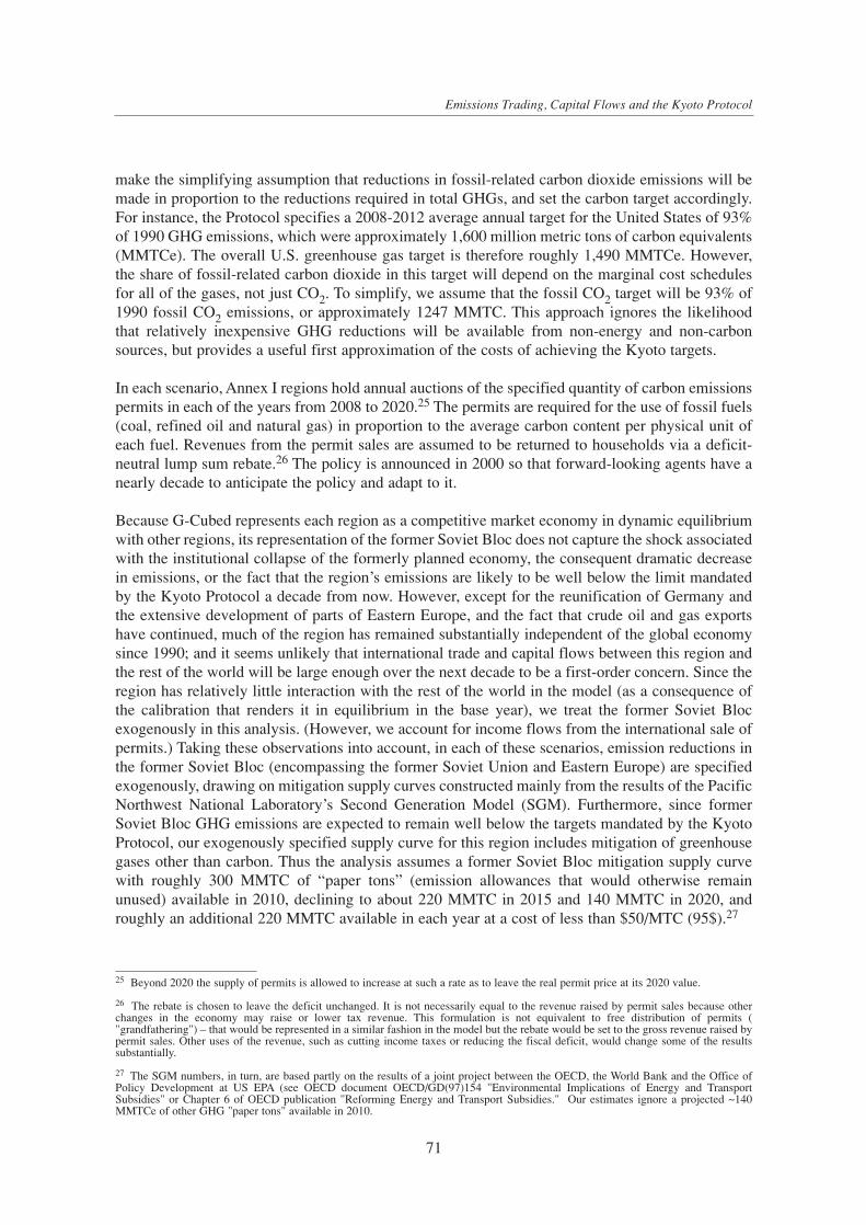
make the simplifying assumption that reductions in fossil-related carbon dioxide emissions will bemade in proportion to the reductions required in total GHGs, and set the carbon target accordingly.For instance, the Protocol specifies a 2008-2012 average annual target for the United States of 93%of 1990 GHG emissions, which were approximately 1,600 million metric tons of carbon equivalents(MMTCe). The overall U.S. greenhouse gas target is therefore roughly 1,490 MMTCe. However,the share of fossil-related carbon dioxide in this target will depend on the marginal cost schedulesfor all of the gases, not just CO2. To simplify, we assume that the fossil CO2 target will be 93% of1990 fossil CO2 emissions, or approximately 1247 MMTC. This approach ignores the likelihoodthat relatively inexpensive GHG reductions will be available from non-energy and non-carbonsources, but provides a useful first approximation of the costs of achieving the Kyoto targets.
In each scenario, Annex I regions hold annual auctions of the specified quantity of carbon emissionspermits in each of the years from 2008 to 2020.25 The permits are required for the use of fossil fuels(coal, refined oil and natural gas) in proportion to the average carbon content per physical unit ofeach fuel. Revenues from the permit sales are assumed to be returned to households via a deficit-neutral lump sum rebate.26 The policy is announced in 2000 so that forward-looking agents have anearly decade to anticipate the policy and adapt to it.
Because G-Cubed represents each region as a competitive market economy in dynamic equilibriumwith other regions, its representation of the former Soviet Bloc does not capture the shock associatedwith the institutional collapse of the formerly planned economy, the consequent dramatic decreasein emissions, or the fact that the region’s emissions are likely to be well below the limit mandatedby the Kyoto Protocol a decade from now. However, except for the reunification of Germany andthe extensive development of parts of Eastern Europe, and the fact that crude oil and gas exportshave continued, much of the region has remained substantially independent of the global economysince 1990; and it seems unlikely that international trade and capital flows between this region andthe rest of the world will be large enough over the next decade to be a first-order concern. Since theregion has relatively little interaction with the rest of the world in the model (as a consequence ofthe calibration that renders it in equilibrium in the base year), we treat the former Soviet Blocexogenously in this analysis. (However, we account for income flows from the international sale ofpermits.) Taking these observations into account, in each of these scenarios, emission reductions inthe former Soviet Bloc (encompassing the former Soviet Union and Eastern Europe) are specifiedexogenously, drawing on mitigation supply curves constructed mainly from the results of the PacificNorthwest National Laboratory’s Second Generation Model (SGM). Furthermore, since formerSoviet Bloc GHG emissions are expected to remain well below the targets mandated by the KyotoProtocol, our exogenously specified supply curve for this region includes mitigation of greenhousegases other than carbon. Thus the analysis assumes a former Soviet Bloc mitigation supply curvewith roughly 300 MMTC of “paper tons” (emission allowances that would otherwise remainunused) available in 2010, declining to about 220 MMTC in 2015 and 140 MMTC in 2020, androughly an additional 220 MMTC available in each year at a cost of less than $50/MTC (95$).27
71
Emissions Trading, Capital Flows and the Kyoto Protocol
25 Beyond 2020 the supply of permits is allowed to increase at such a rate as to leave the real permit price at its 2020 value.
26 The rebate is chosen to leave the deficit unchanged. It is not necessarily equal to the revenue raised by permit sales because otherchanges in the economy may raise or lower tax revenue. This formulation is not equivalent to free distribution of permits ("grandfathering") – that would be represented in a similar fashion in the model but the rebate would be set to the gross revenue raised bypermit sales. Other uses of the revenue, such as cutting income taxes or reducing the fiscal deficit, would change some of the resultssubstantially.
27 The SGM numbers, in turn, are based partly on the results of a joint project between the OECD, the World Bank and the Office ofPolicy Development at US EPA (see OECD document OECD/GD(97)154 "Environmental Implications of Energy and TransportSubsidies" or Chapter 6 of OECD publication "Reforming Energy and Transport Subsidies." Our estimates ignore a projected ~140MMTCe of other GHG "paper tons" available in 2010.
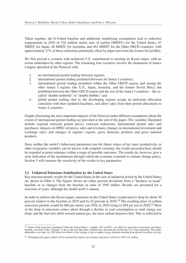
Taken together, the G-Cubed baseline and additional simplifying assumptions lead to reductionrequirements in 2010 of 526 million metric tons of carbon (MMTC) for the United States, 67MMTC for Japan, 48 MMTC for Australia, and 461 MMTC for the Other OECD countries; withapproximately 27% of those reductions potentially offset by paper tons from the former Soviet Bloc.
We first present a scenario with unilateral U.S. commitment to meeting its Kyoto target, with noaction undertaken by other regions. The remaining four scenarios involve the attainment of AnnexI targets specified in the Protocol with:
1. no international permit trading between regions;2. international permit trading permitted between all Annex I countries;3. international permit trading permitted within the Other OECD region, and among the
other Annex I regions (the U.S., Japan, Australia, and the former Soviet Bloc), butprohibited between the Other OECD region and the rest of the Annex I countries – the so-called “double umbrella” or “double bubble;” and
4. global permit trading; that is, the developing regions accept an emissions allocationconsistent with their modeled baselines, and allow sales from their permit allocations toAnnex I countries.
Graphs illustrating the most important impacts of the Protocol under different assumptions about theextent of international permit trading are provided at the end of the paper. The variables illustratedinclude regional emission permit prices; emission reductions; international permit sales andpurchases; impacts on OPEC oil prices, sales and revenues; changes in international investment andexchange rates; and changes in regions’ exports, gross domestic products and gross nationalproducts.
Since neither the model’s behavioral parameters nor the future values of tax rates, productivity, orother exogenous variables can be known with complete certainty, the results presented here shouldbe regarded as point estimates within a range of possible outcomes. The results do, however, give aclear indication of the mechanisms through which the economy responds to climate change policy.Section 5 will examine the sensitivity of the results to key parameters.
3.1 Unilateral Emissions Stabilization by the United StatesKey macroeconomic results for the United States in the case of unilateral action by the United Statesare shown in Table 4. The figures shown are either percent deviations from a “business as usual”baseline or as changes from the baseline in units of 1995 dollars. Results are presented for aselection of years, although the model itself is annual.
In order to achieve the Kyoto target, emissions in the United States would need to drop by about 30percent relative to the baseline in 2010 and by 42 percent in 2020.28 The resulting price of carbonemissions permits would be $80 per metric ton (95$) in 2010 rising to $94 per ton in 2020.29 Mostof the drop in emissions comes about through a decline in coal consumption as total energy usedrops and the fuel mix shifts toward natural gas, the least carbon-intensive fuel. This is reflected in
Warwick J. McKibbin, Martin T. Ross, Robert Shackleton, and Peter J. Wilcoxen
72
28 Some of the emissions eliminated within the United States – roughly 10% in 2010 – are offset by increases in emissions elsewhere.Initially, over half of this "leakage" is due to the fact that other countries buy and burn the oil that the U.S. stops importing. This effectdiminishes over time: by 2020 about two-thirds of the leakage is due to higher energy demand resulting from greater economic activity.
29 Throughout the paper carbon will be measured in metric tons (tonnes) and prices will be in 1995 U.S. dollars.
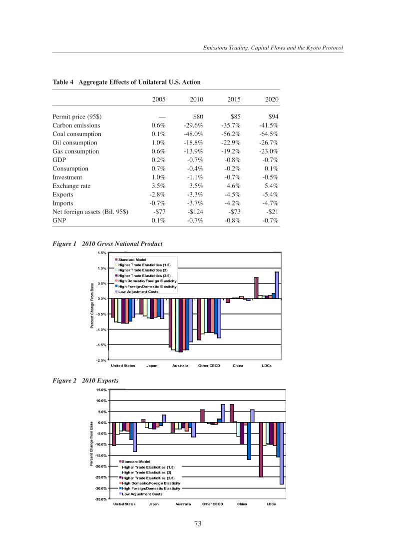
73
Emissions Trading, Capital Flows and the Kyoto Protocol
Table 4 Aggregate Effects of Unilateral U.S. Action
2005 2010 2015 2020
Permit price (95$) — $80 $85 $94Carbon emissions 0.6% -29.6% -35.7% -41.5%Coal consumption 0.1% -48.0% -56.2% -64.5%Oil consumption 1.0% -18.8% -22.9% -26.7%Gas consumption 0.6% -13.9% -19.2% -23.0%GDP 0.2% -0.7% -0.8% -0.7%Consumption 0.7% -0.4% -0.2% 0.1%Investment 1.0% -1.1% -0.7% -0.5%Exchange rate 3.5% 3.5% 4.6% 5.4%Exports -2.8% -3.3% -4.5% -5.4%Imports -0.7% -3.7% -4.2% -4.7%Net foreign assets (Bil. 95$) -$77 -$124 -$73 -$21GNP 0.1% -0.7% -0.8% -0.7%
Figure 15: 2010 Gross National Product
-2.0%
-1.5%
-1.0%
-0.5%
0.0%
0.5%
1.0%
1.5%
United States Japan Australia Other OECD China LDCs
Per
cent
Cha
nge
From
Bas
e
Standard Model
Higher Trade Elasticities (1.5)
Higher Trade Elasticities (2)
Higher Trade Elasticities (2.5)
High Domestic/Foreign Elasticity
High Foreign/Domestic Elasticity
Low Adjustment Costs
Figure 16: 2010 Exports
-35.0%
-30.0%
-25.0%
-20.0%
-15.0%
-10.0%
-5.0%
0.0%
5.0%
10.0%
15.0%
United States Japan Australia Other OECD China LDCs
Per
cent
Cha
nge
from
Bas
e
Standard Model
Higher Trade Elasticities (1.5)
Higher Trade Elasticities (2)
Higher Trade Elasticities (2.5)
High Domestic/Foreign Elasticity
High Foreign/Domestic Elasticity
Low Adjustment Costs
Figure 1 2010 Gross National Product
Figure 2 2010 Exports

the industry-level results shown in Table 5: the after-tax price of coal rises by more than 235 percentrelative to its baseline level, while coal output declines by 40 percent in 2010 and by 56 percent in2020. Output of petroleum products falls by 16% in 2010 and 24% in 2020; while natural gas outputfalls by 14% in 2010 and 23% in 2020. The crude oil and gas sector is somewhat less affected,suggesting that declines in demand fall disproportionately on imports: domestic output declines by10 to 20 percent over the period.
Outside the energy industries, prices and output are affected very little. The only noteworthy resultis that investment rises by about one percent during the period before the policy is implemented(2000-2007). This stems from the fact that the demand for services increases slightly whenhouseholds and firms substitute away from energy. As a result, investment by the service industryincreases as well, in anticipation of the increase in demand. The increase in investment is financedby an inflow of foreign capital, as aggregate national savings decline slightly. The capital inflowcauses the exchange rate to appreciate by about 3.5 percent over that period. The exchange rateappreciation reduces exports, primarily of durable goods, and enables the capital inflow to bereflected in a worsening of the current account.
The international effects of the US policy vary across regions. Most Annex I countries experiencemild decreases in GDP on the order of -0.1 percent, mild exchange rate depreciation, and increasesin their net investment positions. China’s exports rise by 4 to 6 percent in the early years of thepolicy. Other developing countries receive minor capital inflows after 2010, experience very slightexchange rate appreciation and end up with slightly higher GDPs, but also have lower productionand exports of durable goods due to the change in exchange rates.
3.2 Annex I Targets Met Without International Permit TradingIn the second scenario, all Annex I regions meet their commitments under the Protocol. Each regionis restricted to use of their allocated emissions; the permits can be traded within regions but not from
Warwick J. McKibbin, Martin T. Ross, Robert Shackleton, and Peter J. Wilcoxen
74
Table 5 Industry Effects of Unilateral U.S. Action
2005 2010 2020
Price Qty Price Qty Price QtyEnergy IndustriesElectric utilities -0.1% 0.4% 7.2% -6.2% 12.6% -9.5%Gas utilities -0.2% 0.4% 14.3% -13.6% 26.0% -22.7%Petroleum refining -0.5% 0.4% 19.6% -16.2% 27.6% -24.4%Coal mining 0.1% -0.1% 235.4% -40.3% 375.6% -56.0%Oil and gas extraction -0.2% 0.0% -8.1% -10.4% -7.0% -19.7%Other SectorsOther mining -0.4% -0.3% 0.7% -2.6% 0.7% -3.3%Agriculture -0.3% 0.2% -0.2% -1.2% -0.7% -0.8%Forestry and wood -0.4% 0.1% -0.4% -1.2% -0.9% -1.0%Durable goods -0.6% -0.2% -0.6% -1.4% -1.2% -1.4%Nondurables -0.3% 0.3% -0.5% -1.0% -0.9% -0.6%Transportation -0.2% 0.3% -0.1% -1.6% -0.6% -1.3%Services -0.2% 0.4% -0.9% -0.2% -1.4% 0.5%

one region to another.30 This simulation allows us to measure the heterogeneity of the Annex Iregions. Differences in baseline emissions growth, endowments of fossil fuels, reliance on fossilfuels for energy generation and initial fossil fuel prices mean that the regions face substantiallydifferent costs of achieving stabilization. This will be reflected in the pattern of permit prices (whichwill indicate the cost of stabilization at the margin) and GDP losses across regions.
The results for the Annex I policy without international permit trading are shown in Table 6. Keyresults are presented for 2005, 2010 and 2020 for the four OECD regions in the model (United
75
Emissions Trading, Capital Flows and the Kyoto Protocol
30 Even though there is no trading between regions, trading is implicitly allowed between the countries within a region. In particular, the"Other OECD" region lumps together the European Union, Canada and New Zealand, so trading is implicitly allowed between thesecountries.
Table 6 Annex I Commitments Without International Permit Trading
United Japan Australia Other China LDC’sStates OECD
2005Permit price (95$) — — — — — — Carbon emissions 1.9% -2.4% -0.1% -1.8% -0.9% 1.7%Coal consumption 0.7% -0.8% 0.0% -0.6% -0.8% 0.2%Oil consumption 3.1% -3.3% -0.1% -2.4% -1.0% 2.6%Gas consumption 1.9% -0.7% 0.0% -1.5% -1.5% 1.8%GDP 0.4% -0.3% 0.1% -0.2% -0.3% 0.3%Investment 2.9% -0.5% 0.6% -2.0% -1.0% 2.7%Exports -8.6% 3.4% -0.3% 7.6% 17.2% -21.5%Exchange rate 10.8% -6.5% 0.7% -12.9% -4.7% 15.4%Net foreign assets (Bil. 95$) -$244 -$49 $16 $184 $20 $78GNP 0.3% -0.3% 0.1% 0.0% -0.2% 0.5%
2010Permit price (95$) $87 $112 $181 $261 — — Carbon emissions -29.6% -20.6% -37.5% -32.7% -0.7% 3.3%Coal consumption -51.9% -43.6% -55.1% -49.6% -0.8% 0.3%Oil consumption -15.6% -14.2% -18.4% -29.5% -0.4% 5.1%Gas consumption -12.6% -4.6% -19.4% -18.2% -1.2% 3.4%GDP -0.4% -0.6% -1.8% -1.5% -0.2% 0.4%Investment 0.8% -1.3% 0.2% -3.8% -0.4% 2.9%Exports -10.7% 1.2% -4.5% 5.8% 8.1% -25.1%Exchange rate 10.5% -5.8% 2.1% -13.5% -4.7% 15.9%Net foreign assets (Bil. 95$) -$451 -$55 $29 $370 $34 $141GNP -0.6% -0.5% -1.6% -1.3% -0.1% 0.7%
2020Permit price (95$) $101 $162 $230 $315 — — Carbon emissions -35.7% -27.6% -44.1% -39.1% -0.7% 3.1%Coal consumption -59.7% -56.5% -64.7% -58.4% -0.7% 0.2%Oil consumption -19.8% -19.6% -21.2% -35.1% -0.4% 4.8%Gas consumption -17.9% -6.7% -23.9% -24.0% -1.1% 3.4%GDP -0.5% -0.7% -1.8% -1.6% -0.2% 0.4%Investment 0.9% -1.4% 0.3% -3.5% -0.7% 2.5%Exports -12.2% 1.3% -6.7% 4.1% 4.7% -20.7%Exchange rate 11.0% -7.0% 5.0% -13.0% -5.0% 15.7%Net foreign assets (Bil. 95$) -$489 -$104 $48 $490 $43 $184GNP -0.7% -0.7% -1.5% -1.3% -0.1% 0.7%

States, Japan, Australia and other OECD, hereafter referred to as ROECD), as well as China and theless developed countries (LDCs).
The effects of the policy differ substantially across the regions: in 2010, permit prices per metric tonof carbon range from a low of $87 in the US to a high of $261 in the ROECD region. These resultsshow that both marginal and average costs of abating carbon emissions differ substantially across
countries. Since, by assumption, all regions have access to the same technologies, the differences inpermit prices reflect differences in mitigation opportunities: regions which have relatively lowbaseline carbon emissions per unit of output, and are thus relatively sparing in their use of fossilfuels, have relatively fewer options for reducing emissions further. The differences among regionsstem in part from differences in the fuel mix but also depend on the availability of alternative fuelsand the extent to which baseline emissions rise above the stabilization target. Thus Australia, whichhas relatively few substitution possibilities and a high baseline emission trajectory (due to fairlyhigh population growth and strong productivity growth) finds it costly to reach the 1990stabilization target. The United States, with low energy prices, a high reliance on coal and abundantnatural gas, finds it relatively cheap to change the composition of energy inputs. The table shows results for both GDP and GNP. The GDP results indicate the extent of internationalshifts in production but are a poor measure of national welfare. The GNP figures are a better(although far from perfect) welfare measure because GNP reflects the total income accruing to theresidents of a country, including net income transfers to and from factors of production locatedabroad. Savers in countries with high costs of abatement shift some of their financial capitaloverseas, maintaining rates of return that otherwise would be much lower. The ordering of countriesby GNP loss is the same as that by GDP loss but the dispersion of GNP losses is smaller because ofthe ability of agents to shift capital into higher return activities abroad.
The effect on GDP follows a pattern similar to that of mitigation costs: GDP in 2010 falls slightlyin the US and Japan while in Australia and ROECD it falls by 1.8 and 1.5 percent, respectively.Comparing this simulation with the previous one shows that the United States is better off under theAnnex I policy than it is when it reduces emissions on its own: in 2010, U.S. GDP 0.4 percent belowits baseline value while under the unilateral policy it would have fallen by 0.7 percent. One reasonfor the lower costs is that U.S. exports are more competitive relative to those from other OECDeconomies when more countries impose carbon constraints. Another reason for the reduction inGDP loss lies in the fact that the United States has substantially lower marginal costs of abatingcarbon emissions than other OECD economies. Stabilizing emissions requires a smaller priceincrease in the U.S. than it does in other countries. Also the policy directly reduces rates of returnin each economy, and relatively more so in sectors that are relatively carbon intensive. Lowerabatement costs in the U.S. mean that rates of return to capital in the U.S. fall less than in otherOECD countries. This shift in rates of return induces investors to shift their portfolios toward U.S.assets, leading to an increase in U.S. investment. Thus, production tends to fall less in the U.S. thanit does in other OECD economies. The effect is particularly apparent in the years immediatelybefore the policy takes effect: U.S. investment is three percent above baseline in 2005. In addition,the U.S. also benefits from lower world oil prices as Annex I oil demand falls. The boost ininvestment and lower oil prices both tend to raise energy demand and cause permit prices to riserelative to the unilateral stabilization scenario – from $80 to $87 in 2010 and from $94 to $101 in2020. U.S. income, as measured by GNP, rises slightly in the period before the policy takes effectand then falls by 0.5 to 0.6 percent in 2010-2020.
Examining the effect of the policy on different regions raises a number of interesting results that tendto be ignored in popular discussion of the impacts of emission permit trading. Those regions that have
Warwick J. McKibbin, Martin T. Ross, Robert Shackleton, and Peter J. Wilcoxen
76

the largest relative abatement costs, such as Australia and ROECD, have large capital outflows becauseof the fall in the rate of return to capital in high abatement cost countries. ROECD, which faces thegreatest cost of stabilizing emissions, has a large capital outflow, accumulating to roughly $490 billion(95$) by 2020. Most of this capital outflow goes to the United States, and some also goes to developingcountries, which are not controlling emissions at all. Capital flows to developing countries are limitedby adjustment costs, however: it is expensive for a region with a relatively small capital stock to absorba large flow of new capital.31 It is relatively cheap for a large country such as the United States toabsorb capital for the same reason: the costs of a given absolute change in a particular capital stockdecrease with the size of the stock. Thus, relatively small capital inflows can exhaust arbitrageopportunities in developing economies. This is an important insight because it contradicts the popularperception that greenhouse abatement policies will lead to wholesale migration of industries fromdeveloped countries to non-abating developing countries. Our results show this is quite unlikely;moreover, most of the financial capital reallocation is between OECD economies.Capital flows cause the exchange rates of countries receiving financial capital, such as the UntiedStates and developing countries, to appreciate, and cause the Japanese and ROECD currencies todepreciate. The dollar appreciates by 25 percent relative to the ROECD currencies, but depreciatesby 5 percent relative to the currency of developing countries. The ROECD currency depreciates by30 percent relative to the developing countries. These changes lead directly to changes in exportpatterns. By 2010, ROECD exports of durable goods increase by about 6 percent over baselinewhile U.S. exports of durables fall by 11 percent. At the same time, capital flows cause Australianand ROECD GNP to fall by less slightly than GDP, since these countries’ increased foreigninvestments offset some of the lost income from domestic production.
Overall, the effect of achieving the Kyoto targets is to reduce GDP in countries with high abatementcosts, cause an outflow of capital, depreciate their exchange rates and stimulate exports. The effecton low-cost countries is the opposite: capital inflows tend to raise GDP by reducing real interestrates and stimulating domestic demand in the short run, and by raising the capital stock in themedium to long run. Capital inflows also appreciate the exchange rate and diminish exports.
The effect of the Protocol on developing countries is particularly interesting. In the case of theLDCs, the exchange rate appreciation has multiple costs and benefits. Exports become lesscompetitive but imports become cheaper and the dollar value of LDC international debt fallsdramatically, leading to a net improvement in the LDCs’ net international investment position inspite of significant capital inflows, as mentioned above. LDC gross domestic product rises by threepercent in 2010, and gross national product rises by 0.7 percent. Clearly, the absence ofcommitments under the Kyoto Protocol confers significant benefits to LDCs through internationalpolicy transmission.
In addition, the decline in Annex I oil demand leads to a 10 percent decline in OPEC oil exports anda 17 percent decline in world oil prices. The decline in oil prices benefits the LDCs, whose increasedoil consumption causes an increase in LDC carbon emissions equivalent to approximately 6 percentof Annex I emission reductions. This 6 percent “leakage effect,” however, does not translate intoincreased LDC exports of carbon-intensive durable goods, which are significantly dampened by theimpact of capital inflows on LDC exchange rates. Instead it is the region most adversely affected bymitigation policy – ROECD – which experiences an increase in exports. It may seem surprising thatexport performance should improve in the country most hurt by climate change policy but it is
77
Emissions Trading, Capital Flows and the Kyoto Protocol
31 In apparent contradiction to this statement, the results in Table 6 show an apparent net capital outflow from the LDCs rather than acapital inflow. The improvement in the LDCs’ net foreign asset position is due to the fact that their real exchange rate appreciation leadsto a decrease in the dollar value of their outstanding debt. The decrease in the value of outstanding debt outweighs policy-induced thecapital inflow, leading to an apparent capital outflow.
simply the result of consistent international accounting: countries which experience capital outflowsmust experience trade surpluses, while countries which experience capital inflows must experiencetrade deficits.
3.3 Annex I International Permit TradingThe third scenario is identical to the second except that we allow international trading in emissionspermits among Annex I countries. The effect of allowing trading is twofold. First, arbitrage willcause the price of a permit to be equal in all Annex I countries. This will ensure that marginal costsof carbon abatement will be equal across countries and that Annex I emission reductions will beachieved at minimum cost. Countries with relatively low abatement costs will sell permits and abatemore than in the previous scenario; countries with high costs will buy permits and undertake lessdomestic abatement.
In addition, trading makes possible a relaxation of the overall constraint during the 2008-2012period because the emissions of one Annex I region, the former Soviet Bloc, are likely to be belowthe limit specified under the Protocol. The relaxation of the constraint means that actual emissionreductions under the Protocol will be considerably lower – perhaps as much as 40% lower – withinternational permit trading than without it, at least during the first budget period. The particularcircumstances of the former Soviet Bloc thus make it difficult to determine the pure gains frompermit trading, independent of the relaxation of the constraint.32
Results for this scenario are shown in Table 7. In contrast to independent mitigation, internationalpermit trading leads to a uniform permit price throughout the Annex I that rises from about $61 perton in 2010 to $109 per ton in 2020. These prices, lower than any OECD region’s marginalmitigation cost in the absence of international permit trading, lead to lower increases in fossil fuelprices and considerably lower domestic reductions than in the previous case since reductions can beavoided by purchasing allowances from the former Soviet Bloc. At the 2010 permit price of $61 perton, the former Soviet Bloc sells not only its excess allowances, 293 MMTC, but also reducesemissions to sell an additional 253 MMTC of allowances. Thus the OECD countries purchase nearly550 MMTC of emission allowances from the former Soviet Bloc rather than undertake domesticreductions, thereby dramatically reducing the cost of meeting their commitments. These purchasesparticularly benefit ROECD, which uses internationally purchased allowances to meet 72 percent ofits obligations and thus achieves a 77 percent reduction in its marginal abatement costs. The UnitedStates and Australia use internationally purchased allowances to meet 29 percent and 65 percent oftheir respective obligations, and benefit from 30 percent and 66 percent reductions in marginalabatement costs. International purchases of former Soviet Bloc allowances amount to nearly $33billion (95$) in 2010 and rise to nearly $54 billion by 2020.
Interestingly, as the regional economies continue to grow after 2010, the demand for emissionallowances increases while the former Soviet Bloc’s willingness to supply them declines. As aconsequence, international permit prices rise continuously after 2010, and by 2020, prices rise to$109 per ton. At this price, the United States becomes a net permit seller, supplying about 83MMTC of allowances to Japan, Australia and ROECD at a total cost of nearly $9 billion, and takingan equivalent quantity of domestic emission reductions in excess of its international commitment.
Warwick J. McKibbin, Martin T. Ross, Robert Shackleton, and Peter J. Wilcoxen
78
32 Previous analysis using the G-Cubed model indicates that the pure gains from trade are on the order of 20 to 25 percent in the caseOECD international permit trading. See McKibbin, Shackleton and Wilcoxen (1998b).

The economic impacts of the Protocol are generally significantly reduced by both the equalizationof marginal mitigation costs and permit prices under an international permit trading regime, as wellas by the reduction in overall mitigation due to the sale of former Soviet Bloc’s excess allowances.U.S. GDP costs in 2010 are cut from 0.4 percent to 0.2 percent. Japanese GDP costs are cut from0.6 percent to 0.4 percent, Australia’s from 1.8 percent to 0.7 percent, and ROECD’s from 1.5percent to 0.6 percent. Permit trading has little effect on non-participants: results for China and thedeveloping countries are very similar to the no-trading case.
79
Emissions Trading, Capital Flows and the Kyoto Protocol
Table 7 Annex I Commitments With International Permit Trading
United Japan Australia Other China LDC’sStates OECD
2005Permit price (95$) — — — — — — Annual permit sales (Bil. 95$) — — — — — — Carbon emissions 1.4% -2.7% -0.3% -2.1% -0.6% 1.8%Coal consumption 0.6% -1.0% -0.3% -0.6% -0.6% 0.2%Oil consumption 2.3% -3.7% -0.7% -2.9% -0.8% 2.7%Gas consumption 1.5% -0.7% -0.8% -1.7% -1.2% 1.9%GDP 0.3% -0.2% 0.0% -0.2% -0.2% 0.3%Investment 2.3% -0.6% -0.3% -2.2% -0.6% 3.0%Exports -6.9% 3.6% 1.1% 8.9% 11.5% -22.8%Exchange rate 8.9% -7.1% -0.6% -14.4% -2.4% 16.6%Net foreign assets (Bil. 95$) -$139 -$28 $22 $242 $16 $67GNP 0.2% -0.2% 0.0% -0.1% -0.2% 0.5%
2010Permit price (95$) $61 $61 $61 $61 — — Annual permit sales (Bil. 95$) -$9.4 -$1.5 -$1.9 -$20.3 — — Carbon emissions -20.9% -13.0% -13.0% -9.1% -0.5% 2.6%Coal consumption -36.0% -24.2% -18.7% -12.1% -0.5% 0.4%Oil consumption -11.8% -10.4% -6.7% -9.0% -0.4% 4.0%Gas consumption -8.8% -2.9% -6.8% -5.6% -0.7% 2.9%GDP -0.2% -0.4% -0.7% -0.6% -0.1% 0.4%Investment 0.8% -1.0% -0.3% -2.4% -0.3% 2.8%Exports -7.6% 2.5% -0.8% 8.0% 5.7% -23.7%Exchange rate 8.5% -6.7% -0.4% -14.7% -2.1% 17.5%Net foreign assets (Bil. 95$) -$304 -$12 $36 $476 $29 $121GNP -0.5% -0.4% -0.8% -0.6% -0.1% 0.7%
2020Permit price (95$) $109 $109 $109 $109 — — Annual permit sales (Bil. 95$) $9.0 -$4.4 -$4.6 -$53.7 — — Carbon emissions -33.3% -18.6% -18.4% -13.0% -0.4% 2.7%Coal consumption -54.5% -35.4% -26.8% -17.8% -0.4% 0.4%Oil consumption -19.9% -14.3% -9.2% -12.3% -0.3% 4.2%Gas consumption -16.6% -4.5% -10.0% -8.3% -0.6% 3.1%GDP -0.5% -0.5% -0.9% -0.7% -0.1% 0.5%Investment 0.5% -1.1% -0.2% -2.4% -0.4% 2.7%Exports -9.1% 2.2% -1.9% 7.3% 2.7% -20.2%Exchange rate 9.1% -7.1% 0.5% -15.0% -2.1% 17.9%Net foreign assets (Bil. 95$) -$390 -$22 $47 $614 $40 $165GNP -0.7% -0.5% -1.1% -0.7% 0.0% 0.7%

Exchange rate changes are similar in sign but generally larger in magnitude than under the no-trading scenario. The Japanese and ROECD currencies, in particular, depreciate somewhat more,while the currency of the developing region has a larger appreciation. This happens because thecountries buying permits must ultimately pay for them with additional exports, either immediatelyor in the future. Thus, the purchasing country’s current account must eventually move towardsurplus by an amount corresponding to the value of the permits.33 The changes in real exchangerates are necessary to accommodate the changes in trade balances.
Permit trading reduces the OECD’s overall GNP costs of meeting their commitments under theKyoto Protocol by about 63 percent in 2010, from $272 billion to $128 billion, or by $143 billion.34
On the basis of previous analysis using G-Cubed of OECD permit trading without former SovietBloc participation, we estimate that roughly 60 percent of these benefits are due to relaxation of theconstraint, while the other 40 percent constitute true gains from trade. If we also take into accountthe spillover effects on China and the LDCs, the world GNP costs of meeting Kyoto commitmentsis cut by 52 percent from $241 billion to $115 billion, or by $125 billion. These 2010 GNP gainsare very unequally dispersed, however: the U.S.35 gains only $14 billion, and Australia and Japanonly $5 billion each; while the ROECD region gains $102 billion. Chinese and LDC GNPs arealmost completely unaffected.
3.4 The “Double Umbrella”In the fourth scenario, the ROECD countries engage in exclusive permit trading and the rest of theAnnex I countries engage in permit trading independently of the ROECD countries. Results fromthis scenario are contained in Table 8. The key difference between this scenario and full Annex Itrading is that ROECD no longer buys 327 million tonnes worth of permits from the former SovietBloc. As a result, the effects on ROECD look much like the no-trading case and abatement costs inthe rest of Annex I fall substantially. Permit prices fall to $32 in 2010 and $71 in 2020. The U.S.benefits in two ways: from lower permit prices and also from relatively large capital flows fromROECD to the U.S (because high energy prices reduce returns to capital in ROECD). As a result,U.S. GDP remains at its baseline level in 2010 and falls by only 0.2 percent in 2020.
It is interesting to note that the ROECD region is slightly better off in the initial years of the doubleumbrella simulation than under Annex I trading. In 2005, GDP and GNP are slightly higher (thatis, they fall slightly less), fuel consumption and investment are both higher, and capital outflows aresmaller. The reason for this is somewhat subtle. When the ROECD region adopts carbon controlsunder either simulation, one effect is to shift some investment to other regions, especially the UnitedStates. Under Annex I trading, other countries are also subject to relatively tight carbon controlsand are attempting to do the same thing. This causes the U.S. dollar to appreciate substantially,rising by 23% relative to the ROECD currency in 2005. Under the double umbrella, however,carbon controls are much looser in regions other than the ROECD so there is less competition toshift capital into the United States. There is less appreciation of the dollar, which rises by only 16%relative to the ROECD currency. This makes it less expensive for ROECD investors to convert partof their portfolios to U.S. investments.
Warwick J. McKibbin, Martin T. Ross, Robert Shackleton, and Peter J. Wilcoxen
80
33 This shifting of resources between economies due to changes in property rights is known in international economics as the "transferproblem," and is the subject of a large literature dating back to the early 1920s when the effects of German war reparations were hotlydebated.
34 We do not provide estimates of GNP effects for the former Soviet Bloc because of the difficulties mentioned previously.
35 The U.S. experiences a small GDP loss from trading in 2010, due to business cycle effects stemming from our assumption that wagesadjust slowly: the sharp increase in U.S. energy prices under the trading scenario temporarily reduces labor demand relative to the no-trading case, leading to a decline in GDP.

This is entirely a short run effect, however. Once the policy is actually in force, the ROECD is hurtmore by high abatement costs under the double umbrella than it gains from changes in the terms oftrade. By 2010, ROECD GDP and GNP are about 0.8% below what they would have been underAnnex I trading.
81
Emissions Trading, Capital Flows and the Kyoto Protocol
Table 8 Annex I Commitments With “Double Umbrella”
United Japan Australia Other China LDC’sStates OECD
2005Permit price (95$) — — — — — —
Annual permit sales (Bil. 95$) — — — — — — Carbon emissions 1.2% -2.0% -0.3% -1.3% -0.5% 1.1%Coal consumption 0.5% -0.7% 0.0% -0.5% -0.5% 0.1%Oil consumption 1.9% -2.9% -0.7% -1.8% -0.6% 1.8%Gas consumption 1.2% -0.6% -0.4% -1.1% -0.9% 1.3%GDP 0.3% -0.2% -0.1% -0.1% -0.2% 0.2%Investment 1.8% -0.5% -0.5% -1.4% -0.6% 1.9%Exports -5.4% 3.2% 1.1% 5.3% 10.5% -14.8%Exchange rate 6.9% -5.7% -1.3% -9.1% -2.7% 10.5%Net foreign assets (Bil. 95$) -$137 -$18 $20 $139 $13 $53GNP 0.2% -0.2% 0.0% 0.0% -0.1% 0.3%
2010Permit price (95$) $32 $32 $32 $263 — — Annual permit sales (Bil. 95$) -$11.4 -$1.6 -$1.3 — — — Carbon emissions -9.2% -5.7% -6.7% -32.7% -0.4% 2.2%Coal consumption -18.2% -11.9% -9.6% -49.8% -0.4% 0.3%Oil consumption -3.3% -4.1% -3.2% -29.5% -0.3% 3.4%Gas consumption -3.1% -1.5% -3.6% -18.1% -0.7% 2.2%GDP 0.0% -0.3% -0.4% -1.4% -0.1% 0.3%Investment 1.3% -0.6% -0.2% -3.4% -0.2% 2.0%Exports -6.9% 1.9% -0.5% 4.3% 5.3% -16.7%Exchange rate 6.6% -5.4% -1.3% -9.3% -2.5% 11.0%Net foreign assets (Bil. 95$) -$281 -$1 $32 $298 $23 $103GNP -0.2% -0.2% -0.5% -1.3% -0.1% 0.5%
2020Permit price (95$) $71 $71 $71 $318 — — Annual permit sales (Bil. 95$) -$19.8 -$5.7 -$3.9 — — — Carbon emissions -18.6% -10.4% -11.0% -39.9% -0.3% 2.2%Coal consumption -32.3% -21.3% -16.1% -60.0% -0.4% 0.3%Oil consumption -9.6% -7.3% -5.3% -35.7% -0.2% 3.5%Gas consumption -8.5% -2.6% -6.1% -24.2% -0.4% 2.4%GDP -0.2% -0.3% -0.6% -1.5% -0.1% 0.3%Investment 0.7% -0.8% -0.3% -3.1% -0.3% 1.8%Exports -7.7% 1.7% -1.2% 2.4% 2.7% -14.5%Exchange rate 6.2% -6.0% -1.3% -8.4% -2.8% 10.7%Net foreign assets (Bil. 95$) -$363 -$15 $41 $440 $29 $141GNP -0.5% -0.3% -0.7% -1.3% 0.0% 0.5%
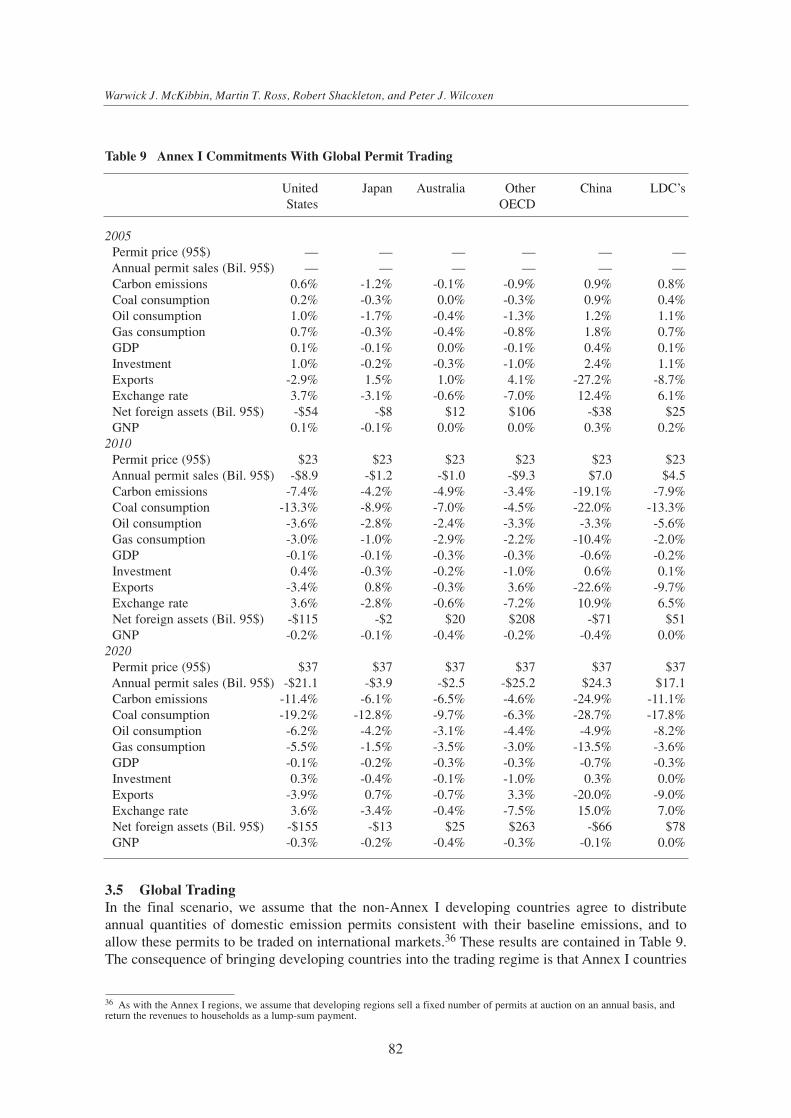
3.5 Global TradingIn the final scenario, we assume that the non-Annex I developing countries agree to distributeannual quantities of domestic emission permits consistent with their baseline emissions, and toallow these permits to be traded on international markets.36 These results are contained in Table 9.The consequence of bringing developing countries into the trading regime is that Annex I countries
Warwick J. McKibbin, Martin T. Ross, Robert Shackleton, and Peter J. Wilcoxen
82
Table 9 Annex I Commitments With Global Permit Trading
United Japan Australia Other China LDC’sStates OECD
2005Permit price (95$) — — — — — — Annual permit sales (Bil. 95$) — — — — — — Carbon emissions 0.6% -1.2% -0.1% -0.9% 0.9% 0.8%Coal consumption 0.2% -0.3% 0.0% -0.3% 0.9% 0.4%Oil consumption 1.0% -1.7% -0.4% -1.3% 1.2% 1.1%Gas consumption 0.7% -0.3% -0.4% -0.8% 1.8% 0.7%GDP 0.1% -0.1% 0.0% -0.1% 0.4% 0.1%Investment 1.0% -0.2% -0.3% -1.0% 2.4% 1.1%Exports -2.9% 1.5% 1.0% 4.1% -27.2% -8.7%Exchange rate 3.7% -3.1% -0.6% -7.0% 12.4% 6.1%Net foreign assets (Bil. 95$) -$54 -$8 $12 $106 -$38 $25GNP 0.1% -0.1% 0.0% 0.0% 0.3% 0.2%
2010Permit price (95$) $23 $23 $23 $23 $23 $23Annual permit sales (Bil. 95$) -$8.9 -$1.2 -$1.0 -$9.3 $7.0 $4.5Carbon emissions -7.4% -4.2% -4.9% -3.4% -19.1% -7.9%Coal consumption -13.3% -8.9% -7.0% -4.5% -22.0% -13.3%Oil consumption -3.6% -2.8% -2.4% -3.3% -3.3% -5.6%Gas consumption -3.0% -1.0% -2.9% -2.2% -10.4% -2.0%GDP -0.1% -0.1% -0.3% -0.3% -0.6% -0.2%Investment 0.4% -0.3% -0.2% -1.0% 0.6% 0.1%Exports -3.4% 0.8% -0.3% 3.6% -22.6% -9.7%Exchange rate 3.6% -2.8% -0.6% -7.2% 10.9% 6.5%Net foreign assets (Bil. 95$) -$115 -$2 $20 $208 -$71 $51GNP -0.2% -0.1% -0.4% -0.2% -0.4% 0.0%
2020Permit price (95$) $37 $37 $37 $37 $37 $37 Annual permit sales (Bil. 95$) -$21.1 -$3.9 -$2.5 -$25.2 $24.3 $17.1Carbon emissions -11.4% -6.1% -6.5% -4.6% -24.9% -11.1%Coal consumption -19.2% -12.8% -9.7% -6.3% -28.7% -17.8%Oil consumption -6.2% -4.2% -3.1% -4.4% -4.9% -8.2%Gas consumption -5.5% -1.5% -3.5% -3.0% -13.5% -3.6%GDP -0.1% -0.2% -0.3% -0.3% -0.7% -0.3%Investment 0.3% -0.4% -0.1% -1.0% 0.3% 0.0%Exports -3.9% 0.7% -0.7% 3.3% -20.0% -9.0%Exchange rate 3.6% -3.4% -0.4% -7.5% 15.0% 7.0%Net foreign assets (Bil. 95$) -$155 -$13 $25 $263 -$66 $78GNP -0.3% -0.2% -0.4% -0.3% -0.1% 0.0%
36 As with the Annex I regions, we assume that developing regions sell a fixed number of permits at auction on an annual basis, andreturn the revenues to households as a lump-sum payment.

can purchase emission allowances from owners in developing countries. These owners, in turn,would be willing to sell allowances to Annex I buyers only if the allowance price exceeded themarginal cost to the owners of undertaking emission reductions within the developing countries.The market process would thus lead to least cost reductions on a global scale: emission reductionswould be taken wherever they are cheapest, but Annex I countries would pay for them.
Full global trading cuts the permit cost to $23 per metric ton of carbon (MTC) in 2010 and $37 perMTC in 2020, and has minor GDP effects in the Annex I economies, ranging from less than -0.1%for the U.S. and Japan to –0.3% for Australia and the ROECD. In 2010, the OECD regions achieve75 to 90 percent of their targets through international purchases of emission allowances. Moreover,since wider availability of emission allowances reduces permit prices, OECD regions are able topurchase international permits at a lower overall cost than in the preceding scenarios: in 2010,international permit sales total $20 billion in the global trading case, about 60% of the $33 billionvalue of former Soviet Bloc international permit sales in the Annex I trading case. China providesabout 300 MMTC of these allowances, and the other LDCs provide about 195 MMTC; the formerSoviet Bloc provides another 410 MMTC. Nearly all of the reductions in China and the LDCs areachieved through reductions in coal use. Thus, one of the crucial effects of expanding from anAnnex I trading regime to global trading is to transfer mitigation from oil-related emissions to coal.As a result, oil exporting countries experience only very modest losses in exports and revenues.Finally, global trading eliminates the possibility of carbon leakage.
The reduction in mitigation costs and the equalization of mitigation costs across regions greatlyreduces the international macroeconomic effects of the Kyoto Protocol, compared with the previousscenarios. Except for Australia, OECD regions experience GDP and GNP impacts of at most 0.4percent. Capital flows, exchange rate impacts and trade effects are all considerably lower. Relativeto the no-trading case, aggregate OECD GNP costs in 2010 are cut by 78 percent from $233 billionto $51 billion; and relative to the Annex I trading case, costs are cut by 59 percent. All OECDregions benefit from cost reductions.
Relative to scenarios in which they do not participate in controlling emissions, the developingcountries are significantly worse off because they no longer experience significant capital inflows,exchange rate appreciations, reductions in the value of their debt burdens, or lower oil prices. GDPin the LDC region falls by 0.2 percent relative to baseline in 2010 instead of rising as it does underthe other simulations. Similarly, China’s GDP is also lower under global trading than under the otherregimes. In terms of GNP, participating in global trading costs the LDCs $26 billion in 2010 relativeto both the Annex I no-trading and Annex I trading cases. These results suggest that that the AnnexI countries may have to use part of their savings ($73 billion in 2010 from moving from Annex Itrading to global trading) simply to induce the developing countries to participate in helping themmeet their commitments under the Protocol.
4 Alternative Revenue Recycling Mechanisms
The preceding results are all based on the assumption that countries that undertake commitments toauction emission permits and return the revenues to households in lump-sum payments. We haveused the G-Cubed model to perform additional scenarios, using alternative assumptions about thedistribution of permits and/or recycling of revenues37. While we do not present those results in
83
Emissions Trading, Capital Flows and the Kyoto Protocol
37 See McKibbin and Wilcoxen (1995b) for results on recycling assumptions using an earlier version of the model.

detail here, we note that the results suggest that alternative revenue recycling mechanisms that serveto increase national savings and/or investment do not have any substantial impact on the marginalcosts of meeting targets (under any given set of rules about international permit trading), but canhave substantially different international macroeconomic effects. For example, when permitrevenues are used to reduce fiscal deficits or increase fiscal surpluses, regions’ national savingsincrease and the global cost of capital falls. Changes in the cost of capital leads to different netinternational capital flows, exchange rate impacts, and GDP/GNP effects. Extending this insight, wenote that the distribution of costs and benefits may be substantially affected if regions pursuediffering policies, for example if some regions pursue revenue recycling policies that encouragesaving and investment and other regions pursue policies that encourage current consumption. Weintend to explore these issues further in continued work with the model.
5 Sensitivity Analysis
The results discussed in the preceding sections are conditional on a range of assumptions built intothe model. For a model like G-Cubed, which focuses on trade and capital flows, two particularlyimportant sets of parameters are those governing the responsiveness of trade to changes in the pricesof traded goods (the “Armington” elasticities) and those governing the ease with which investmentcan increase industries’ stocks of physical capital (capital stock adjustment cost parameters). In thissection we examine how changes in these parameters affect both the baseline case and policyscenario results. To keep the discussion manageable, we focus only on the case which the Annex Iregions achieve their targets without international permit trading. Because it involves the largestinternational responses to carbon targets, this No-trade case provides the greatest illumination of thesensitivity of the results to parameter assumptions.
There are two sets of Armington trade elasticities in the model, one specifying the elasticity ofsubstitution between domestic and foreign goods, and the other specifying substitutability betweenalternative sources of foreign goods. In our standard model, we set both of these elasticities to unity.For comparison, we have conducted two groups of sensitivity analyses: one group which we set bothelasticities at values of 1.5, 2.0 and 2.5, and another in which we set one of the elasticities at 1.0 andthe other at 2.0. The first group of analyses reveals the importance of the overall responsiveness oftrade to policy shocks while the second reveals relative importance of the two tiers in determiningthat responsiveness.
Like the trade elasticities, the capital stock adjustment cost parameters can strongly influence theresults. In our standard model, we specify an adjustment cost parameter f of 0.4. In our sensitivity,we reduce the parameter to 0.2. For an economy with net investment equal to 10% of the capitalstock, this sensitivity implies reducing adjustment costs from 20% to 10% of net investment. Withthese lower adjustment costs it is cheaper to expand a sector’s capital stock, all else being equal.Furthermore, for regions with relatively small initial capital stocks, this sensitivity can imply adramatic reduction in the costs of rapidly expanding the capital stock through foreign investmentinflows.
The results for the No-trade scenarios are contained in Table 10 and Table 11, which show,respectively, the effects of varying the parameters on baseline case variables and policy case results.First, higher Armington elasticities permit large baseline capital outflows from developed regions(with relatively modest investment opportunities) to developing regions with greater prospects forproductivity growth. This has concomitant effects on the regions’ gross domestic and national
Warwick J. McKibbin, Martin T. Ross, Robert Shackleton, and Peter J. Wilcoxen
84
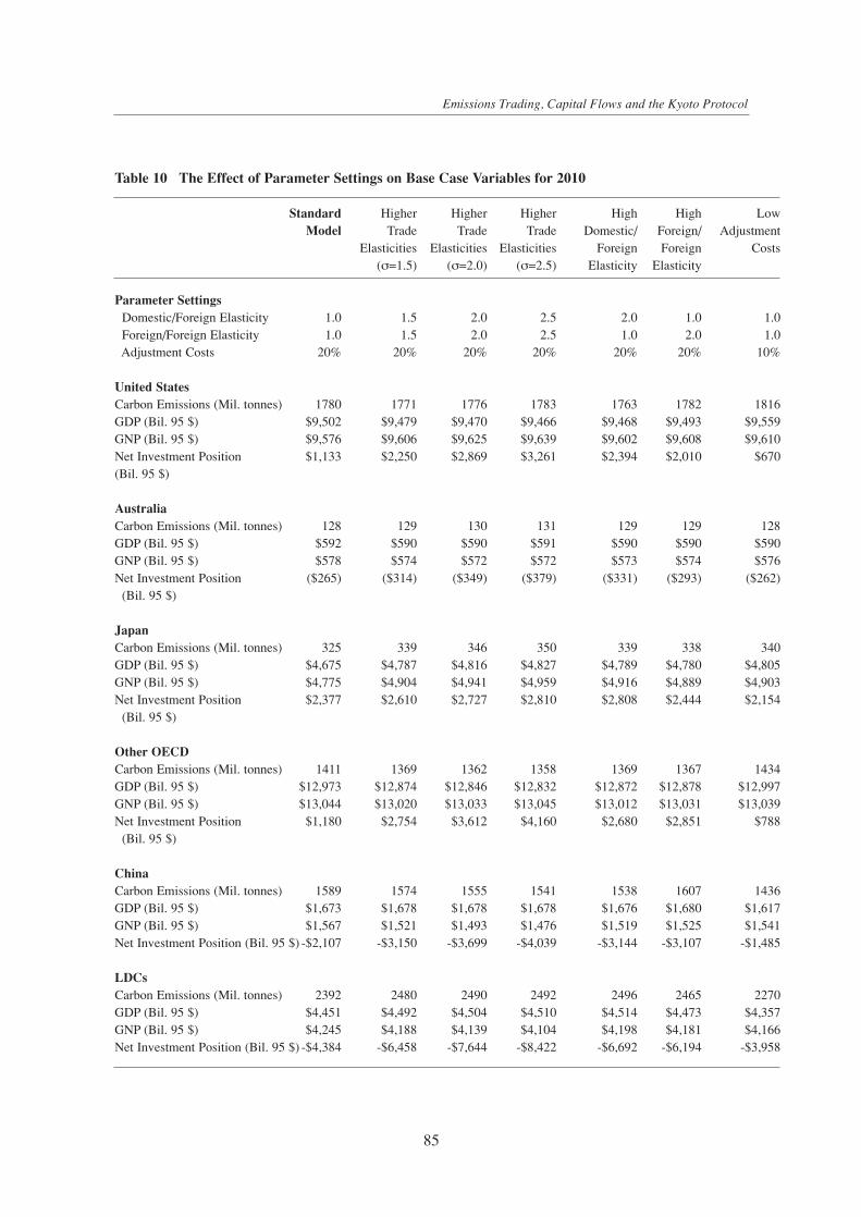
85
Emissions Trading, Capital Flows and the Kyoto Protocol
Table 10 The Effect of Parameter Settings on Base Case Variables for 2010
Standard Higher Higher Higher High High LowModel Trade Trade Trade Domestic/ Foreign/ Adjustment
Elasticities Elasticities Elasticities Foreign Foreign Costs(σ=1.5) (σ=2.0) (σ=2.5) Elasticity Elasticity
Parameter SettingsDomestic/Foreign Elasticity 1.0 1.5 2.0 2.5 2.0 1.0 1.0Foreign/Foreign Elasticity 1.0 1.5 2.0 2.5 1.0 2.0 1.0Adjustment Costs 20% 20% 20% 20% 20% 20% 10%
United StatesCarbon Emissions (Mil. tonnes) 1780 1771 1776 1783 1763 1782 1816GDP (Bil. 95 $) $9,502 $9,479 $9,470 $9,466 $9,468 $9,493 $9,559 GNP (Bil. 95 $) $9,576 $9,606 $9,625 $9,639 $9,602 $9,608 $9,610Net Investment Position $1,133 $2,250 $2,869 $3,261 $2,394 $2,010 $670 (Bil. 95 $)
AustraliaCarbon Emissions (Mil. tonnes) 128 129 130 131 129 129 128GDP (Bil. 95 $) $592 $590 $590 $591 $590 $590 $590 GNP (Bil. 95 $) $578 $574 $572 $572 $573 $574 $576Net Investment Position ($265) ($314) ($349) ($379) ($331) ($293) ($262)
(Bil. 95 $)
JapanCarbon Emissions (Mil. tonnes) 325 339 346 350 339 338 340GDP (Bil. 95 $) $4,675 $4,787 $4,816 $4,827 $4,789 $4,780 $4,805 GNP (Bil. 95 $) $4,775 $4,904 $4,941 $4,959 $4,916 $4,889 $4,903Net Investment Position $2,377 $2,610 $2,727 $2,810 $2,808 $2,444 $2,154
(Bil. 95 $)
Other OECDCarbon Emissions (Mil. tonnes) 1411 1369 1362 1358 1369 1367 1434GDP (Bil. 95 $) $12,973 $12,874 $12,846 $12,832 $12,872 $12,878 $12,997 GNP (Bil. 95 $) $13,044 $13,020 $13,033 $13,045 $13,012 $13,031 $13,039Net Investment Position $1,180 $2,754 $3,612 $4,160 $2,680 $2,851 $788
(Bil. 95 $)
ChinaCarbon Emissions (Mil. tonnes) 1589 1574 1555 1541 1538 1607 1436GDP (Bil. 95 $) $1,673 $1,678 $1,678 $1,678 $1,676 $1,680 $1,617GNP (Bil. 95 $) $1,567 $1,521 $1,493 $1,476 $1,519 $1,525 $1,541Net Investment Position (Bil. 95 $) -$2,107 -$3,150 -$3,699 -$4,039 -$3,144 -$3,107 -$1,485
LDCsCarbon Emissions (Mil. tonnes) 2392 2480 2490 2492 2496 2465 2270GDP (Bil. 95 $) $4,451 $4,492 $4,504 $4,510 $4,514 $4,473 $4,357GNP (Bil. 95 $) $4,245 $4,188 $4,139 $4,104 $4,198 $4,181 $4,166Net Investment Position (Bil. 95 $) -$4,384 -$6,458 -$7,644 -$8,422 -$6,692 -$6,194 -$3,958

Warwick J. McKibbin, Martin T. Ross, Robert Shackleton, and Peter J. Wilcoxen
86
Table 11 The Effect of Parameter Settings on No-Trade Results for 2010
Standard Higher Higher Higher High High LowModel Trade Trade Trade Domestic/ Foreign/ Adjustment
Elasticities Elasticities Elasticities Foreign Foreign Costs(σ=1.5) (σ=2.0) (σ=2.5) Elasticity Elasticity
Parameter SettingsDomestic/Foreign Elasticity 1.0 1.5 2.0 2.5 2.0 1.0 1.0Foreign/Foreign Elasticity 1.0 1.5 2.0 2.5 1.0 2.0 1.0Adjustment Costs 20% 20% 20% 20% 20% 20% 10%
United StatesCarbon Permit Price (95 $) $87 $83 $83 $83 $81 $85 $93Carbon Emissions Change (MMTC) -526 -517 -523 -529 -510 -528 -562GDP, % change -0.4% -0.7% -0.8% -0.8% -0.7% -0.6% -0.3%GNP, % change -0.6% -0.8% -0.8% -0.8% -0.8% -0.7% -0.6%Change in Net Investment -$451 -$233 -$137 -$77 -$257 -$306 -$675
(Bil. 95 $)Real Exchange Rate, % change 10.5% 3.3% 1.8% 1.1% 1.9% 5.7% 13.5%
JapanCarbon Permit Price (95 $) $112 $147 $159 $164 $146 $145 $128Carbon Emissions Change (MMTC) -67 -81 -89 -92 -81 -80 -82GDP, % change -0.6% -0.5% -0.6% -0.6% -0.5% -0.6% -0.8%GNP, % change -0.5% -0.6% -0.6% -0.7% -0.6% -0.6% -0.6%Change in Net Investment -$55 -$59 -$67 -$71 -$100 -$55 -$26
(Bil. 95 $)Real Exchange Rate, % change -5.8% 0.7% 1.0% 0.9% 0.6% -0.2% -9.9%
AustraliaCarbon Permit Price (95 $) $181 $182 $185 $188 $181 $184 $181Carbon Emissions Change (MMTC) -48 -49 -50 -50 -49 -49 -48GDP, % change -1.8% -2.0% -2.1% -2.1% -2.0% -2.0% -1.5%GNP, % change -1.6% -1.7% -1.7% -1.7% -1.7% -1.7% -1.4%Change in Net Investment $29 $37 $38 $38 $39 $37 $13
(Bil. 95 $)Real Exchange Rate, % change 2.1% -0.2% 0.1% 0.4% 0.0% 0.3% 4.8%
Other OECDCarbon Permit Price (95 $) $261 $248 $246 $244 $249 $246 $269Carbon Emissions Change (MMTC) -461 -419 -412 -409 -419 -417 -484GDP, % change -1.5% -1.2% -1.2% -1.2% -1.2% -1.3% -1.5%GNP, % change -1.3% -1.1% -1.1% -1.1% -1.1% -1.1% -1.3%Change in Net Investment $370 $220 $160 $122 $240 $274 $516
(Bil. 95 $)Real Exchange Rate, % change -13.5% -2.4% -0.9% -0.3% -1.4% -4.4% -17.1%
ChinaCarbon Emissions Change (MMTC) -12 -3 -2 -1 -3 -4 -15GDP, % change -0.2% -0.1% 0.0% 0.0% 0.0% -0.1% -0.2%GNP, % change -0.1% 0.0% 0.0% 0.0% 0.1% 0.0% -0.1%Change in Net Investment $34 $18 $12 $8 $17 $20 $59
(Bil. 95 $)Real Exchange Rate, % change -4.7% -2.2% -1.5% -1.3% -1.9% -2.4% -6.5%
LDCsCarbon Emissions Change (MMTC) 79 38 38 39 38 41 96GDP, % change 0.4% 0.0% 0.0% 0.0% 0.0% 0.1% 0.6%GNP, % change 0.7% 0.1% 0.1% 0.1% 0.1% 0.2% 0.9%Change in Net Investment $144 $56 $38 $29 $110 $89 $171
(Bil. 95 $)Real Exchange Rate, % change 15.9% 0.1% -0.8% -1.0% 0.5% 1.0% 23.7%

products, trade, and carbon emissions. Second, this result is influenced by both trade elasticities,although the “top-tier” elasticity of substitution between domestic and foreign goods plays asomewhat greater role in easing baseline capital flows than that between imports from differentregions.
Third, note that lower capital stock adjustment costs make it easier for a region to expand its owndomestic capital stock. Although intuition suggests that lower adjustment costs might make it easierto invest in developing countries with small capital stocks, and thus further encourage capital flowsto developing regions, the opposite appears to be the case: lower adjustment costs also make it easierfor regions to expand their own capital stocks. Thus lower adjustment costs tend to reduce baselineinternational capital flows rather than increase them, and consequently tend to reduce growthprospects in developing regions as well.
Finally, note that Japanese carbon emissions are significantly higher in baselines with higher tradeelasticities. In all the baselines, Japan’s real exchange rate depreciates over the next two decades aslarge quantities of capital flow out of Japan in favor of higher returns in developing countries. Withlow trade elasticities, the real exchange rate depreciation makes fossil fuels more expensive andtends to moderate energy and carbon emissions. With higher trade elasticities, capital outflows donot have as large an effect on the exchange rate. Since the exchange rate depreciates less, fossil fuelimports are relatively cheaper, which leads to higher Japanese baseline carbon emissions. Highercarbon emissions, finally, require a higher permit price to achieve the Japanese target specified bythe Kyoto Protocol.
The policy case sensitivities in Table 11 reveal a number of interesting insights. Perhaps mostimportantly, larger trade elasticities dramatically reduce the exchange rate adjustment required togenerate a capital movement of given magnitude. This is not surprising, since the exchange ratechange acts on both imports and exports. As a result, the effect of doubling the Armington elasticityis to cut the exchange rate adjustment required to transfer a given quantity of financial capital byroughly a factor of four. Greater trade responsiveness also reduces the need to relocate physicalcapital stocks. As a result, the higher the trade elasticities are, the smaller the net foreign asset flowsout of regions with high control costs to regions with low or no control costs.
Because higher trade elasticities moderate both capital flows and exchange rate responses to a givenset of carbon emission mitigation policies, they have rather dramatic effects on the distribution ofcosts across regions. With higher trade elasticities, neither the United States nor the developingcountries benefit as much from capital inflows and the resulting improvements in their terms oftrade. Consequently, developing countries’ GDP and GNP gains from mitigation policies in theAnnex I region are dramatically reduced, and U.S. losses are significantly greater. The ROECDregion experiences significantly lower declines, and China, which is harmed by Annex I policywhen trade elasticities are low, experiences no harm when they are relatively high.
Interestingly, (although we omit the results from the tables to save space) we note that with highertrade elasticities, it is no longer the case that the ROECD region benefits (in the sense of havingsmaller exchange rate effects and consumption losses) from having the rest of the Annex I form atrading bloc that excludes it. With higher elasticities, and the resulting moderation in exchange rateand capital flow effects, consumption losses are moderated in both the No-Trade and DoubleUmbrella scenarios, and are almost indistinguishable in the two.
Finally, lower capital stock adjustment costs have the opposite effect of higher trade elasticities. Asdescribed above, lower adjustment costs make it easier for a region to expand its own domestic
87
Emissions Trading, Capital Flows and the Kyoto Protocol

capital stock, and therefore tend to reduce foreign investment in the baseline. However, loweringthe adjustment cost parameter has a more profound effect on the investment prospects of developingcountries with small capital stocks than it does on the prospects of large developed countries. As aresult, in the policy cases in which Annex I regions meet Kyoto commitments, all else being equal,lower adjustment costs lead to larger capital flows from the Annex I regions to the developingregions – with concomitantly larger exchange rate effects and GDP and GNP effects.
It thus appears that the key insights of the G-Cubed model still hold under the sensitivitiesconsidered here. It is clear, however, that trade price elasticities and capital stock adjustment costsare important determinants of the magnitudes of capital flow and exchange rate responses to apermit trading regime.
6 Conclusion
The theoretical appeal of an international permits program is strongest if participating countrieshave very different marginal costs of abating carbon emissions – in that situation, the potential gainsfrom trade are largest. Our results show that within the Annex I and globally, abatement costs areindeed quite heterogeneous. The marginal cost of meeting Kyoto targets in the “Rest of the OECD”region is triple that of United States; and large quantities of relatively inexpensive emissionreductions are available from the former Soviet Bloc and non-Annex I developing regions. Thesedifferences in abatement costs are caused by a range of factors including different carbon intensitiesof energy use, different substitution possibilities and different baseline projections of future carbonemissions. Because of these differences, international trading offers large potential benefits toparties with relatively high mitigation costs.
Our results also highlight the potentially important role of international trade and capital flows inglobal responses to the Kyoto Protocol, a role not adequately captured in any other modeling systemof which we are aware. The results suggest that regions that do not participate in permit tradingsystems, or that can reduce carbon emissions at relatively low cost, will benefit from significantinflows of international financial capital under any Annex I policy, with or without trading. Itappears that the United States is likely to experience capital inflows, exchange rate appreciation anddecreased exports. In contrast, the ROECD region, as the highest cost region, will see capitaloutflows, exchange rate depreciation, increased exports of durables and greater GDP losses. Totalflows of capital could accumulate to roughly a half a trillion dollars over the period between 2000and 2020.38 Global participation in a permit trading system would substantially offset theseinternational impacts, but is likely to require additional payments to developing countries to inducethem to forgo the benefits that accrue to them if they do not participate.
Because the model is calibrated to a year in which the former Soviet Bloc and China did notparticipate extensively in global trade, the model effectively assumes that these regions neverexperience extensive capital inflows or outflows. If these regions become fully participatingmembers of the international trade and finance system by 2010, then the international trade andcapital effects in our scenarios would have to be revised. In particular, the capital that flows to theU.S. and LDCs in these scenarios might be spread to the former Soviet Bloc and China too, withmore modest exchange rate and trade balance effects in any given region.
Warwick J. McKibbin, Martin T. Ross, Robert Shackleton, and Peter J. Wilcoxen
88
38 Compare these magnitudes to the more than trillion dollar decline just in the U.S. net international investment position in the pastfifteen years. See the U.S. Government’s Survey of Current Business (July 1998).

The model’s results are also sensitive to assumptions that determine the mitigation cost differencesamong regions. Different results would be obtained if U.S. domestic mitigation costs weresignificantly higher but the other regions’ permit prices were on the same order of magnitude as inthese scenarios (this is the case, for example, in the SGM model from which we derive mitigationcost curves for the former Soviet Bloc). With a smaller relative control cost differential between theU.S. and other countries in the OECD, the magnitude of capital flows to the U.S., and the costs andbenefits of those flows, would all be smaller.
Finally, it must be remembered that there are inescapable uncertainties in the values of the model’sbehavioral parameters and the future values of exogenous variables. As shown by our sensitivityanalysis, our results should be interpreted as point estimates in a range of possible outcomes. It isclear, however, that in an increasingly interconnected world in which international financial flowsplay a crucial role, the impact of greenhouse abatement policy cannot be determined without payingattention to the impact of these policies on the return to capital in different economies. Focusingonly on domestic effects would miss a crucial part of the economy’s response to climate changepolicy. To understand the full adjustment process to international greenhouse abatement policy it isessential to model international capital flows explicitly.
89
Emissions Trading, Capital Flows and the Kyoto Protocol

References
Armington, (1969), “A Theory of Demand for ProductsDistinguished by Place of Production,” InternationalMonetary Fund Staff Papers, vol. 16, pp. 159-76.
Bagnoli, Philip, Warwick J. McKibbin, and Peter J.Wilcoxen (1996) “Future Projections and StructuralChange,” in N. Nakicenovic, W. D. Nordhaus, R.Richels and F. L. Toth (eds.), Climate Change:Integrating Science, Economics, and Policy, Laxenburg,Austria: International Institute for Applied SystemsAnalysis, pp. 181-206.
Campbell J. And N. G. Mankiw (1990) “PermanentIncome, Current Income and Consumption”, Journal ofBusiness and Economic Statistics, 8(2), pp. 265-79.
Feldstein, Martin and Charles Horioka (1980), “DomesticSavings and International Capital Flows,” The EconomicJournal, 90, pp. 314-29.
Flavin, M. A. (1981), “The Adjustment of Consumption toChanging Expectations about Future Income,” Journalof Political Economy, 89, pp. 974-1009.
Gordon, Roger H. and A. Lans Bovenberg (1994), “Why isCapital so Immobile Internationally? PossibleExplanations and Implications for Capital Taxation”,mimeo, July.
Goulder, Lawrence H. (1991), “Effects of Carbon Taxes inan Economy with Prior Tax Distortions: AnIntertemporal General Equilibrium Analysis for theU.S.,” mimeo, June.
Goulder, Lawrence H. and B. Eichengreen (1989),“Savings Promotion, Investment Promotion, andInternational Competitiveness,” in Rob Feenstra (ed.),Trade Policies for International Competitiveness,Chicago: University of Chicago Press.
Gurvich, E., A. Golub, A. Mukhin, M. Uzyakov and M.Ksenofontov (1997), “Greenhouse Gas Impacts ofRussian Energy Subsidies” in Reforming Energy andTransport Subsidies: Environmental and EconomicImplications, Paris: Organization for Economic Co-operation and Development.
Hall, R. E. (1978), “Stochastic Implications of the Life-Cycle Hypothesis: Theory and Evidence,” Journal ofPolitical Economy, 86, pp. 971-987.
Hayashi, F. (1979) “Tobin’s Marginal q and Average q: ANeoclassical Interpretation.” Econometrica 50, pp.213-224.
Hayashi, F. (1982) “The Permanent Income Hypothesis:Estimation and Testing by Instrumental Variables.Journal of Political Economy 90(4) pp. 895-916.
Ho, Mun Sing (1989), “The Effects of External Linkageson U.S. Economic Growth: A Dynamic GeneralEquilibrium Analysis”, Ph.D. Dissertation, HarvardUniversity.
Hoel, Michael (1991), “Global Environment Problems:The Effects of Unilateral Actions Taken by OneCountry”, Journal of Environmental Economics andManagement, 20(1), pp. 55-70.
Jorgenson, Dale W. and Peter J. Wilcoxen (1991a),“Reducing U.S. Carbon Dioxide Emissions: The Cost ofDifferent Goals,” in John R. Moroney, ed., Energy,Growth and the Environment, Greenwich, Connecticut:JAI Press, pp. 125-158.
Kalt, J. P. (1985), “The Impact of Domestic EnvironmentalRegulatory Policies on U.S. InternationalCompetitiveness,” Discussion Paper E-85-02, KennedySchool of Government, Harvard University.
Kim J. and L. Lau (1994) “The Role of Human Capital inthe Economic Growth of the East Asian NewlyIndustrialized Countries” paper presented at the Asia-Pacific Economic Modelling Conference, Sydney,August.
Lucas, R. E. (1967), “Optimal Investment Policy and theFlexible Accelerator,” International Economic Review,8(1), pp. 78-85.
Manne, Alan S., and Richard G. Richels (1990), “CO2Emission Limits: An Economic Analysis for the USA,”The Energy Journal, 11(2), 51-74.
Manne, Alan S., and Richard G. Richels (1992), BuyingGreenhouse Insurance - The Economic Costs of CO2Emission Limits, Cambridge, MIT Press.
McKibbin Warwick J. and Jeffrey Sachs (1991) GlobalLinkages: Macroeconomic Interdependence andCooperation in the World Economy, BrookingsInstitution, June.
McKibbin, W. J. and Peter J. Wilcoxen (1995a),“Environmental Policy and International Trade”Brookings Discussion Paper in International Economics#117, The Brookings Institution Washington DC.
McKibbin, Warwick J. and Peter J. Wilcoxen (1995b),“The Theoretical and Empirical Structure of the G-Cubed Model,” Brookings Discussion Paper inInternational Economics #118, The BrookingsInstitution, Washington DC. A revised version of thispaper is forthcoming Economic Modelling.
McKibbin, Warwick J., Robert Shackleton and Peter J.Wilcoxen (1998a), “International Trade and FinancialFlows in a Carbon-Constrained World”, mimeo.
Peck, Stephen and Thomas Teisberg (1990), A Frameworkfor Exploring Cost Effective Carbon Dioxide ControlPaths, Palo Alto, CA: Electric Power Research Institute,October.
Treadway, A. (1969), “On Rational EntrepreneurialBehavior and the Demand for Investment,” Review ofEconomic Studies, 3(2), pp. 227-39.
Uzawa, H. (1969), “Time Preference and the PenroseEffect in a Two Class Model of Economic Growth,”Journal of Political Economy, 77, pp. 628-652.
Warwick J. McKibbin, Martin T. Ross, Robert Shackleton, and Peter J. Wilcoxen
90

Discussion
Ben Geurts
The G-Cubed multi-region, multi-sector intertemporal general equilibrium model of the worldeconomy, as presented by mr. McKibbin, has a number of striking features. The model inhabitsperfect foresight, is claimed to be econometrically estimated and is dynamic in the sense that a year-by-year investment decision is modelled. Moreover capital flows are explicitly modelled. Finallythe model claims to provide information not only about the long-run equilibrium but also about theshort-run dynamics. Each one of these elements would make a general equilibrium model special.Combining them into a single model turns it into a very ambitious and very difficult modellingexercise.
The comments focus on the non-standard elements of the model. The comments are based on therather limited information about the model specification available in the paper. In particular I wouldlike to raise attention to the claim that the model inhabits perfect foresight, to the specification ofthe capital market sub-model and to the short-run dynamics of the model.
The modelling horizon is 2050. Perfect foresight is only possible when, in the end year, the worldis on a steady state growth path. For such an end condition all kind of ratio’s in the model need tobe constant. This, however, is only possible when all kind of growth rates are equal. Since, forinstance, labour supply growth and productivity growth in 2050 have not converged in the model,the model can not be in steady state in 2050, which, in my view, makes it impossible to define theproper end condition.
In the capital market sub-model ad-hoc risk premiums are used to explain the uncovered interest ratedifferentials. The size of these risk premiums is kept constant over the simulation period, butdepends strongly on the choice of the base year. Moreover, at least in the model they are not basedon real or perceived risks. Since there is no risk associated to investment in the model, from awelfare point of view it would be optimal to invest in the most ‘risky’ assets. Moreover the impactof a change in interest rate change on the user cost of capital in a region depends upon the size ofthe risk premium. Since there is no theoretical basis for the risk premiums, and since the empiricalbasis is rather weak, this relationship is rather coincidental. However it seems to be a crucial relationin the model, since the investment reaction determines the capital flows and provokes exchange ratefluctuations. I would like to suggest to elimate gradually over time the risk premiuns, to ensure thatat least in the long run the solution is theoretically optimal.
The third element I like to focus on is the short-run dynamics of the model. The specification of thelabour market, of the consumption function and of the investment decision determine the short rundynamics of the model. From a policy-makers point of view, the short-run dynamics is a veryinteresting feature of the model. Where in general long-run effects of policy measures seem to benegligible, short-run adjustments may be painful. The mere fact that policy makers often seem tofocus on these transition problems, make that they deserve more attention in general equilibriummodels.
91
Emissions Trading, Capital Flows and the Kyoto Protocol

However, at the moment the short term dynamics in the model, are not very sophisticated. To comeup with real short-term dynamics, the model should mimic the stylised fact of the real world thatlong-term elasticity’s are much greater than short-term elasticity’s. This should, for instance, bereflected in the production function and the trade system. A putty-clay production functions, fromthis respect, might be preferable over the CES-production which is used now. In the trading system,elements of the new growth and new trade theories could be included. In specifications based onthese theories regions might be able to growth faster than their competitors in world trade, withoutsuffering from a continuous and ever increasing terms of trade loss. With the long-term tradeelasticity’s which are now in the model, terms-of-trade effects are likely to dominate all other effectson welfare.
As said, the G-cubed model is a very interesting and ambitious model. Although it is not clearwhether the model is already able to meet all the claims of the authors, I look forward to future workon the model, and for actual analyses done with the model.
Ben Geurts
92

Kyoto and Carbon Leakage
simulations with WorldScan
Johannes Bollen, Ton Manders and Hans Timmer
Abstract
The focus of this paper is carbon leakage under the Kyoto protocol. The dynamic AGE modelWorldScan is used to analyse the effects of both unilateral action and permit trading within AnnexI . Two new scenarios, A1 and B1, are used as ‘Business-As-Usual’ scenarios1. The two scenariosturn out to generate similar leakage rates. Furthermore, leakage depends only to a limited extent onthe policy applied. Typical values for the leakage rate turn out to be around 20 percent. Income isless affected than GDP. Important channels through which carbon leakage occurs, are the shift inenergy-intensive production from Annex I towards non-Annex I and the shift within industriestowards cheaper energy in non-Annex I. Crucial for these processes are trade elasticities andproduction substitution elasticities. A sensitivity analyses is done to assess the importance of theseparameters.
1 Introduction
By signing the Kyoto Protocol in December 1997 Annex I countries committed themselves to thereduction of their Greenhouse Gas emissions, with the ultimate goal to stabilize global emissionsand to prevent undesirable climate changes. Although the agreement achieved in Kyoto is animportant first step towards this ultimate goal, it is clear that also emissions outside the group ofAnnex I countries (Non-Annex-I) have to be taken into account to assess the contribution of thisagreement to the stabilization of global emissions. First of all, the relative importance of Annex-Ireductions depends on autonomous increases of emissions in Non-Annex-I. If Annex-I emissionsare a smaller part of global emissions, the relative impact of Annex-I reductions on global emissionsis automatically smaller. Secondly, the impact depends on induced changes in emissions in Non-Annex-I. An increase in Non-Annex-I emissions as a result of mitigation policies in Annex-I, makesthese policies less effective in stabilizing global emissions.
This paper will focus on this induced, so-called leakage effect and especially on carbon leakage. Toassess the order of magnitude of this leakage and to unravel the different causes of leakage we useWorldScan, a dynamic AGE model of the world economy, developed at CPB. Besides leakage ofemissions to countries outside Annex I, leakage may also occur within the Annex I region. The lattermight occur if Annex I countries have emission targets that exceed their expected emissions. This
93
Kyoto and Carbon Leakage
1 Please note that the WorldScan team participated in collaboration with the RIVM IMAGE team in the development of the scenarios forthe IPCC Special Report on Emissions Scenarios (SRES). Calculations in this paper are based on input from the modeling teamsparticipating in SRES and explore how SRES-type scenarios could be used for mitigation analysis. They are necessarily preliminary,since the SRES scenarios have not been approved by IPCC and are therefore subject to changes.

leaves room, often labelled “hot air”, in those countries to increase their emissions as a result ofpolicies in other Annex I countries without violating the Kyoto protocol. This paper will alsoaddress the possible hot air, which is expected only to exist in Russia or the Former Soviet Union.
In the analysis we will split up leakage in three different ways. First, we use the well-known Kayaidentity where a change in emissions is disentangled into a change into a change in production, achange in the energy intensity of production and a change in the carbon intensity of energy.Secondly, we decompose emissions into emissions that are ultimately used for domestic finaldemand and emissions that are use for net exports of goods and services. To that end we computefor all sectors the implicit carbon content, taking into account all intermediate deliveries and allimports. With this decomposition we can compute how mitigation policies change the carboncontent of final demand in Annex-I and Non-Annex-I. Thirdly, in the sensitivity analysis we splitchanges in emissions into changes that result from shifts over sectors and changes that results fromshifts in production technologies.2
There are at least three reasons for leakage. First, as a result of reduced energy demand in Annex-Ithe producer prices of energy in all regions will decline. Cheaper energy in countries that do notadopt mitigation policies will stimulate domestic energy demand. Secondly, energy taxes in AnnexI countries may provoke relocation of energy-intensive production to countries that do not imposeenergy taxes. Thirdly, income effects in non-complying countries may change their domesticenergy demand.3
Taking these transmissions into account we can conclude that the leakage rate will depend on avariety of assumptions. Of overriding importance are assumptions about developments in absenceof mitigation policies, or the so-called business-as-usual (BaU) baseline. In general one can say thatthe larger countries without mitigation policies are, relative to countries that realize reductions ofemissions, and the more they are integrated into the global economy, the larger will be the leakagerate. Large countries can easily absorb a significant amount of extra energy if energy prices decline.Countries that already have a substantial market share in foreign markets and that are open toimports can easily take over a considerable part of energy intensive production from Annex-I. Alsothe degree of integration of energy markets in the baseline is important. If trade in fossil fuels isdifficult and energy markets are more or less regional markets, the energy prices in Non-Annex-Iwill hardly be effected. Finally, if the BaU baseline contains hot air within Annex-I, that willgenerate leakage within Annex-I and as a result the leakage to Non-Annex-I will be smaller.
In this paper we use two scenarios as BaU baselines, acknowledging the fact that there cannot beone “business-as-usual” since the future is inherently unpredictable. These scenarios are based onwork that is ongoing in support of the IPCC Special Report on Emissions Scenarios and the ThirdAssessment Report4. They are referred to as A1 and B1. Both scenarios assume high growth rates,especially in Non-Annex-I. The main difference is that in B1 very rapid autonomous improvementin energy efficiency is assumed. That makes the necessary reductions to comply with the Kyoto
94
Johannes Bollen, Ton Manders and Hans Timmer
2 The distinction between changes in production technologies and shifts over sectors is a vague one. In every economic model sectoraloutput consist of heterogeneous products, which implies that production functions always describe, besides technological options, alsothe consequences of shifts over products. However, in sensitivity analysis the distinction between demand and production functions is aconvenient one because both elements refer to specific model parameters.
3 See also e.g. Oliveira-Martins et.al. (1992).
4 See Footnote 1.
Protocol smaller and it generates a substantial amount of hot air in the Former Soviet Union, evenin 2020. These two scenarios will be described in section 2.
Because in both scenarios are rather similar with respect to the openness of Non-Annex-I and theshare of Non-Annex-I in the world economy, mitigation policies will have similar leakage rates.Because towards 2020 the share of Non-Annex-I in the world economy is steadily increasing, theleakage rate differs more in time than between the two scenarios, albeit that the existence ofsubstantial hot air in the B1 scenario reduces leakage towards Non-Annex-I compared to the A1scenario, where hot air disappears towards the end of the scenario period. Lejour (1999) usesWorldScan to analyse leakage against two other scenarios. These scenarios, developed for theOECD (1997) study, differ significantly with respect to Non-Annex-I. One scenario assumes rapidgrowth of Non-Annex-I regions and further globalization through the lowering of barriers ininternational markets for goods, services and financial capital, while the other scenario is much lessoptimistic about growth and openness of Non-Annex-I. That study shows a significantly largerleakage rate in the first scenario than in the second one.
As starting point of the scenarios we use the GTAP4 database. On the energy side of that databasewe added some extra information and some modifications. We confronted the value of output perregion in GTAP4 with volume data of output provided by the IEA. We assumed that the resultingimplicit price can be seen as a producer price which applies to all categories of demand. Only foroil we made a distinction between the price for domestic sales and exports, using IEA price data onexports and imports of oil. Also that method ensures that the model reproduces the IEA volume dataof energy production per region. Then we calculated indirect taxes on domestic use, irrespectivefrom the suppliers, so that market prices provided by IEA were reproduced. That procedure assumedthat the value data of energy use in GTAP do not contain these indirect taxes. We thereforecomputed new value data including these revealed domestic taxes.
The leakage rate will not only depend on the BaU scenario, but also on the instruments that are usedto reach the targets that Non-Annex-I countries set themselves. In general one can say that the moreefficient the instruments are, the lower the leakage rate will be. Efficient instruments will lead tosmaller distortions and therefore to less relocation of energy-intensive production to Non-Annex-I.In section 3 we consider two policies: unilateral taxes (UNI) and free emission trade within Annex-I (FTR). The later will show a somewhat smaller leakage to Non-Annex-I, because it leads onaverage to smaller price distortions. Both UNI and FTR may induce leakage within Annex-I if hotair exists in the baseline. As far as there is still hot air after unilateral policies, this internal leakagewill be larger in case of free emission trade.
In the implementation of the Kyoto agreement many other instruments may be used besidesunilateral taxes or free trade of emission right within AN-I, but these instruments are beyond thescope of this paper. Some of these instruments we analysed in Bollen et.al. (1999), where wesimulated trade within limited clubs, limits to imports or exports of emission right and projectsunder the clean development mechanism.
To determine the leakage rate, not only the instruments or the magnitude of variables in the baselineare important, but also the assumptions about production possibilities and behavioural relations. Inmodel terms this mainly refers to price elasticities. First of all the price elasticity of energy supplyis a key determinant. Inelastic supply, i.e. small price elasticities, will increase leakage. Suppliers offossil fuels are then prepared to lower their prices drastically in order to maintain output levels asfar as possible after the decline in demand from Non-Annex-I countries. Similarly the priceelasticity of energy demand in Non-Annex-I is an important determinant of leakage. The higher
95
Kyoto and Carbon Leakage

these price elasticities the larger leakage will be, because the easier Non-Annex-I can increaseenergy demand as a result of lower prices. Changes in the price-elasticity of energy demand inAnnex-I, on the other hand, has an opposite effect on the leakage rate. That would provoke largershifts over sectors in the trade patterns. Finally, the price elasticities of trade flows of all goods andservices are important. The higher these elasticities, the larger leakage. High price elasticities inenergy markets imply integrated global energy markets. That means that suppliers of energy in Non-Annex-I are confronted with a decline in demand for their output as a result of mitigation policiesin Annex-I and suppliers of energy in Annex-I can easily shift their sales to Non-Annex-I. Highprice elasticities in other markets facilitate shifts in trade patterns of energy intensive products. Toexplore the impact of some of these price elasticities we present in section 4 some sensitivityanalyses with WorldScan.
Leakage can only occur as a result of trade, trade in energy carriers, or trade in other products.Therefore, to avoid leakage one could see compensating trade policies, like the taxation of energyintensive imports, as an option. Or one could exempt energy-intensive producers in exposed sectorsin Annex-I from carbon taxes. Such counter veiling measures or beyond the scope of the currentpaper. In Tang et.al. (1998) such measures were discussed on the basis of WorldScan simulations.
A short description of WorldScan is given in the appendix. WorldScan contains 12 regions, 6 Annex-I regions and 6 Non-Annex-regions. In this paper we aggregate the results into 4 regions: WesternEurope (WE), Eastern Europe + Former Soviet Union (EF), Rest OECD (RO) and Non-Annex-I(NA).
2 The baselines
The effects of CO2 abatement policies depend on the baseline used. The emission targets set in theKyoto agreement are expressed relative to the emission levels in 1990. The future growth ofemissions, as projected in the baseline, is critical in determining the efforts required to meet theKyoto commitments. There are an infinite number of possible alternative futures to explore. In thispaper we follow two scenarios which have been constructed in support of the Special Report onEmissions Scenarios (SRES) for the IPCC5. These scenarios are described by the names A1 and B1.
The A1 scenario describes a future world of very rapid economic growth, low population growthand rapid introduction of new and more efficient technology. Major underlying themes areconvergence, capacity building and increased cultural and social interactions, with a substantialreduction in regional differences in per capita income. The global economy expands at an averageannual rate of about 3% to 2100.This is approximately the same as average global growth since1850, although the conditions that lead to this global economic growth in productivity and per capitaincomes in the scenario are unparalleled in history. Energy and mineral resources are abundant inthis scenario because of rapid technical progress, which both reduce the resources needed to producea given level of output and increases the economically recoverable reserves. Final energy intensity(energy use per unit of GDP) decreases at an average annual rate of 1.3%. The A1 scenario is basedon a balanced mix of primary energy sources and has an intermediate level of CO2 emissions.
96
Johannes Bollen, Ton Manders and Hans Timmer
5 See Footnote 1.

The B1 scenario describes a convergent world with rapid change in economic structures, andintroduction of clean technologies. The emphasis is on global solutions to environmental and socialsustainability, including concerted efforts for rapid technology development, dematerialization ofthe economy, and improving equity. Global income per capita is somewhat lower than in A1. Ahigher proportion of this income is spent on services rather than on material goods The B1 scenariosees a relatively smooth transition to alternative energy systems as conventional oil and gasresources decline. There is extensive use of conventional and unconventional gas as the cleanestfossil resource during the transition, but the major push is towards post-fossil technologies drivenin large part by environmental concerns.
Basically, the scenarios focus on the long run and certain aspects become manifest only in the farfuture. For example, the strong increase in the use of biofuels and non-thermal electricity in B1takes shape only in the second half of the 21st century. All the same, in the medium run there areimportant differences, especially concerning fossil energy use and CO2 emissions. In this paper ourtime horizon is 2020 and we think it useful to take both baselines A1 and B1 into consideration.
The stories behind these scenarios haven been implemented by different modelling groups (RIVM,1999). This exercise resulted in more detailed trajectories, e.g. for GDP, population, emissions andfuel demand. To mimic the given trends in these scenarios in broad outline, we adjusted in
97
Kyoto and Carbon Leakage
Figure 2.1a Various indicators in A1 scenario(average five year percentage change)
Western Europe EU + FSU
Rest of the OECD non-Annex I
2001-2005 2006-2010 2011-2015 2016-2020 2001-2005 2006-2010 2011-2015 2016-2020
2001-2005 2006-2010 2011-2015 2016-2020 2001-2005 2006-2010 2011-2015 2016-2020
emissionsenergy intensity
gdpcarbon intensity
emissionsenergy intensity
gdpcarbon intensity
emissionsenergy intensity
gdpcarbon intensity
emissionsenergy intensity
gdpcarbon intensity
3
2
1
0
2
0
-4
-2
-6
-8
4
6
8
10
0
2
4
8
6
-1
-1
-2 -2
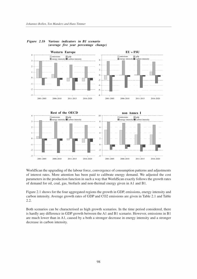
WorldScan the upgrading of the labour force, convergence of consumption patterns and adjustmentsof interest rates. More attention has been paid to calibrate energy demand. We adjusted the costparameters in the production function in such a way that WorldScan exactly follows the growth ratesof demand for oil, coal, gas, biofuels and non-thermal energy given in A1 and B1.
Figure 2.1 shows for the four aggregated regions the growth in GDP, emissions, energy intensity andcarbon intensity. Average growth rates of GDP and CO2 emissions are given in Table 2.1 and Table2.2.
Both scenarios can be characterised as high growth scenarios. In the time period considered, thereis hardly any difference in GDP growth between the A1 and B1 scenario. However, emissions in B1are much lower than in A1, caused by a both a stronger decrease in energy intensity and a strongerdecrease in carbon intensity.
98
Johannes Bollen, Ton Manders and Hans Timmer
Figure 2.1b Various indicators in B1 scenario(average five year percentage change)
Western Europe EU + FSU
Rest of the OECD non Annex Iemissionsenergy intensity
gdpcarbon intensity
emissionsenergy intensity
gdpcarbon intensity
emissionsenergy intensity
gdpcarbon intensity
emissionsenergy intensity
gdpcarbon intensity
2001-2005 2006-2010 2006-20102011-2015 2016-2020 2001-2005 2011-2015 2016-2020
2006-20102001-2005 2011-2015 2016-20202006-20102001-2005 2011-2015 2016-2020
-4
-2
-6
-8
0
2
4
4
3
2
1
0
-1
-2
-3
4
3
2
1
0
-1
-2
-3
10
8
6
4
2
0
-2
-4
6

3 Simulation results
3.1 Emission reductions and carbon taxesIn this section we will discuss two policy scenarios with the A1 scenario as starting point and thesame two policy scenarios with the B1 scenario as starting point. Both policy scenarios impose theKyoto targets on Annex-I emissions. We assumes that the average Kyoto targets for the first budgetperiod will be realized in 2010 and that from 2000 onwards the targets gradually converge from thebaseline emissions to the target in 2010. The targets are kept constant from 2010 till 2020. In thefirst policy scenario the targets of individual regions are reached by unilateral carbon taxes. In thesecond policy scenario free trade of emission rights within Annex-I is allowed, which boils down toa uniform tax in Annex-I to reach the overall Annex-I target, combined with transfer payments as aresult of trade in emission rights.
99
Kyoto and Carbon Leakage
Table 2.1 GDP growth in the A1 and B1 scenarios
1996-2000 2001-2005 2006-2010 2011-2015 2016-2020
A1 average annual growth rate in %Western Europe 3.2 2.9 2.6 2.3 1.9Rest OECD 3.4 3.2 3.1 2.7 2.4EE + FSU 6.2 5.4 5.8 6.0 5.2Rest of the World 7.8 7.8 7.4 7.2 6.6
B1Western Europe 3.2 2.9 2.6 2.3 2.0Rest OECD 3.4 3.2 3.0 2.6 2.4EE + FSU 6.2 5.5 5.7 6.0 5.3Rest of the World 7.8 7.8 7.4 7.2 6.8
Table 2.2 CO2 emissions in the A1 and B1 scenarios
1996-2000 2001-2005 2006-2010 2011-2015 2016-2020
A1 average annual growth rate in %Western Europe 2.6 2.3 1.7 1.0 0.6Rest OECD 1.6 1.0 1.0 0.7 0.2EE + FSU -3.7 -1.2 1.2 2.1 2.9Rest of the World 4.9 5.2 5.1 4.5 4.8
B1Western Europe 2.0 1.6 0.6 -0.6 -0.6Rest OECD 1.1 0.4 0.0 -0.3 -0.7EE + FSU -3.9 -1.7 0.2 0.2 1.5Rest of the World 4.7 5.1 4.9 3.4 3.4

Figure 3.1 shows the resulting emission reductions and carbon prices in 2020. In the A1 scenarioWestern Europe has to reduce its emissions with .6 TgC, which is almost 40% of the emissions inthe baseline. To realize that reduction with unilateral taxes Western Europe needs a carbon tax of121$/tC6. Table 3.1 shows that that tax leads to large increases in the market prices of energy,especially of coal, because the carbon content of coal per US$ is relatively large. Eastern Europeand the Former Soviet Union only have to reduce .06 TgC, about 5% of their baseline emissions.Reductions in the Rest of the OECD are in absolute terms even larger than in Western Europe. Butthe reduction of .7 TgC is only 25% of their baseline. That means that their carbon tax can be lowerthan in Western Europe. Another reason for the relatively low carbon tax is the relatively low energyprices in the Rest of the OECD, especially because of low energy prices in the United States. Thecarbon tax of 50 $/tC leads to relatively large increases in energy prices in the Rest of the OECD.In case of unilateral taxes the carbon leakage in Non-Annex-I is .28 TgC, which is 20% of theAnnex-I reductions. As percentage of the baseline emissions the increase in Non-Annex-I is only3%.
The picture changes radically in case trade in emission rights is allowed. Then the carbon tax is
100
Johannes Bollen, Ton Manders and Hans Timmer
6 $/tC stands for 1995-US dollars per ton carbon
Figure 3.1a Emissions and carbon taxes in A1 scenario
Reductions of emissions (Tg C)
Figure 3.1b Emissions and carbon taxes in B1 scenario
Reductions of emissions (Tg C) Carbon taxes (1995 US $ / tC)
Carbon taxes (1995 US $ / tC)
Western EuropeEastern Europe + FSU non-Annex I
Rest OECD Western EuropeEastern Europe + FSU non-Annex I
Rest OECD
Western EuropeEastern Europe + FSU non-Annex I
Rest OECD Western EuropeEastern Europe + FSU non-Annex I
Rest OECD
0.8
0.6
0.4
0.2
0.0
-0.2
-0.4
0.8
0.6
0.4
0.2
0.0
-0.2
-0.4
0
30
60
90
120
0
30
60
90
120
unilateralemission trade
unilateralemission trade
unilateralemission trade
unilateralemission trade

equal for all Non-Annex-I regions at a level of 42 1995-US$/tC. Because of differences in marginalabatement costs, related to differences in energy prices in the baseline, the impact of this tax onreductions differs across regions. Emissions in Western Europe are reduced by 18% of their baselinelevel (.27 TgC), in EE+FSU by 45% (.46TgC) and in the Rest of the OECD by 21% (.62 TgC). So,compared to the unilateral case it is mainly a shift of reductions from Western Europe to EE+FSU.The leakage in Non-Annex-I is somewhat smaller in case of emission trade because free tradeimplies a more efficient reduction of emissions and less improvement of Non-Annex-Icompetitiveness in energy-intensive goods.
Taking the B1 scenario, with very rapid autonomous increase in energy efficiency, as baseline hastwo major consequences. First of all, for Western Europe and the Rest of the OECD are only aboutone third of the necessary reductions in the A1 scenario. That means that also the carbon tax in thoseregions in the unilateral case are about one third of the levels discussed above. Secondly, EE+FSUhas in the B1 scenario in 2020 a significant amount of hot air, 22% of their baseline emissions or .18 TgC. That means that in the unilateral case there is leakage within Annex-I and EE+FSU will
101
Kyoto and Carbon Leakage
Table 3.1 Real energy prices in 2020 (cumulated % change)
A1 scenario
unilateral emission trade
WE EF RO NA WE EF RO NA
market pricesCoal 90.8 8.1 70.8 -2.3 -2.2 84.1 58.4 -2.2Oil 29.6 5.7 15.5 -2.3 -2.4 79.4 12.5 -2.4Natural Gas 22.3 3.8 16.8 -0.9 -0.9 35.5 13.9 -0.9
producer pr.Coal 0.0 -10.0 -10.9 -1.3 -1.2 -16.8 -9.2 -1.2Oil -2.8 -5.1 -2.0 -2.3 -2.2 -8.9 -2.0 -2.2Natural Gas 0.3 -4.3 -2.8 -0.8 -0.7 -10.0 -2.4 -0.7
B1 scenario
unilateral emission trade
WE EF RO NA WE EF RO NA
market pricesCoal 35.3 -4.4 20.1 -1.1 -0.6 16.4 11.6 -0.6Oil 11.3 -2.4 4.6 -0.8 -0.7 22.6 2.5 -0.7Natural Gas 8.5 -1.3 4.7 -0.3 -0.2 7.1 2.7 -0.2
producer pr.Coal -1.5 -4.4 -5.1 -0.6 -0.3 -2.8 -0.3Oil -1.2 -1.4 -0.7 -0.8 -0.6 -2.8 -0.6 -0.6Natural Gas -0.1 -1.3 -1.4 -0.3 -0.2 -2.4 -0.8 -0.2
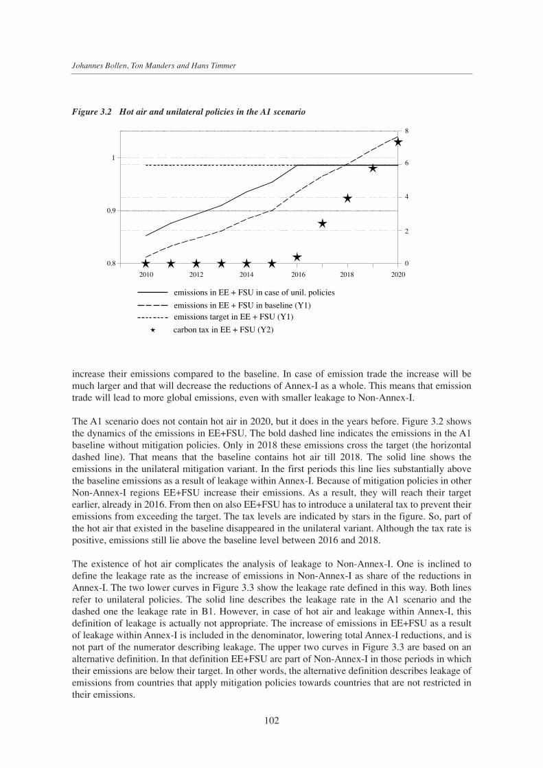
increase their emissions compared to the baseline. In case of emission trade the increase will bemuch larger and that will decrease the reductions of Annex-I as a whole. This means that emissiontrade will lead to more global emissions, even with smaller leakage to Non-Annex-I.
The A1 scenario does not contain hot air in 2020, but it does in the years before. Figure 3.2 showsthe dynamics of the emissions in EE+FSU. The bold dashed line indicates the emissions in the A1baseline without mitigation policies. Only in 2018 these emissions cross the target (the horizontaldashed line). That means that the baseline contains hot air till 2018. The solid line shows theemissions in the unilateral mitigation variant. In the first periods this line lies substantially abovethe baseline emissions as a result of leakage within Annex-I. Because of mitigation policies in otherNon-Annex-I regions EE+FSU increase their emissions. As a result, they will reach their targetearlier, already in 2016. From then on also EE+FSU has to introduce a unilateral tax to prevent theiremissions from exceeding the target. The tax levels are indicated by stars in the figure. So, part ofthe hot air that existed in the baseline disappeared in the unilateral variant. Although the tax rate ispositive, emissions still lie above the baseline level between 2016 and 2018.
The existence of hot air complicates the analysis of leakage to Non-Annex-I. One is inclined todefine the leakage rate as the increase of emissions in Non-Annex-I as share of the reductions inAnnex-I. The two lower curves in Figure 3.3 show the leakage rate defined in this way. Both linesrefer to unilateral policies. The solid line describes the leakage rate in the A1 scenario and thedashed one the leakage rate in B1. However, in case of hot air and leakage within Annex-I, thisdefinition of leakage is actually not appropriate. The increase of emissions in EE+FSU as a resultof leakage within Annex-I is included in the denominator, lowering total Annex-I reductions, and isnot part of the numerator describing leakage. The upper two curves in Figure 3.3 are based on analternative definition. In that definition EE+FSU are part of Non-Annex-I in those periods in whichtheir emissions are below their target. In other words, the alternative definition describes leakage ofemissions from countries that apply mitigation policies towards countries that are not restricted intheir emissions.
102
Johannes Bollen, Ton Manders and Hans Timmer
2010 2012 2014 2016 2018 2020
0
2
4
61
0.9
0.8
8
emissions in EE + FSU in case of unil. policies
emissions in EE + FSU in baseline (Y1)emissions target in EE + FSU (Y1)
carbon tax in EE + FSU (Y2)
Figure 3.2 Hot air and unilateral policies in the A1 scenario

Figure 3.3 shows that the leakage rate hardly differs between the A1 and B1 scenarios. The onlyimportant difference occurs at the end of the scenario period when there is still a substantial amountof hot air in the B1 scenario. The similar leakage rate in both scenarios is a manifestation of a similarrelative size of Non-Annex-I in both scenarios. That the relative size of Non-Annex-I is importantbecomes clear in the analysis of the leakage rate over time. The gradual increase in the leakage rateis the result of the gradual increase in the share of Non-Annex-I in the world economy. Also thelarger leakage rates in the alternative definition are the result of this mechanism. In the alternativedefinition the group of not restricted countries is larger than Non-Annex-I and therefore that groupis responsible for more leakage. Before we investigate emission reductions and carbon leakage infurther detail, first the impact of mitigation policies on production and income will be discussed inthe next subsection.
3.2 Impact on production and incomeFigure 3.4 shows the impact on real gross domestic product (GDP) and real gross national income(GNI ) in 2020 as percentage of the baseline. Unilateral policies in the A1 scenario lead to a declinein European GDP of more than 4%. The forced reduction of energy use can be seen as a negativesupply shock, diminishing the production potential. However, the decline in real GNI is with about0.5 % much less substantial. Change in terms of trade are responsible for 3% of this differencebetween the impact on real GDP and real GNP. As a result of domestic carbon taxes Western Europecan import cheaper energy while it profits from price increases of their exports.
The remaining 0.5 % of the difference is the result of increased net interest income from abroad.That increase is the result of typical current account dynamics after a negative supply side shock.Figure 3.5 shows the investment dynamics in Western Europe. As a result of the (gradual) reductionin production potential the capital stock is adjusted downwards. This implies in the first years asharp decline in investments. Lower investment demand manifests itself in a temporaryimprovement of the trade balance and consequently an improvement of the current account, whichincreases the stock of net wealth invested abroad. As a result, net interest income from abroad rises.
103
Kyoto and Carbon Leakage
2001 2005 2010 2015 2020
0.230
0.180
0.130
0.080
leak
age
rate
A1
B1
A1 + hot air
B1 + hot air
Figure 3.3 Leakage rate

104
Johannes Bollen, Ton Manders and Hans Timmer
Figure 3.4a Impact on production and income in A1 scenario(cumulated % change in 2020)
Unilateral Emission trade
Figure 3.4b Impact on production and income in B1 scenario(cumulated % change in 2020)
Western EuropeEastern Europe + FSU non-Annex I
Rest OECD Western EuropeEastern Europe + FSU non-Annex I
Rest OECD
Western EuropeEastern Europe + FSU non-Annex I
Rest OECD Western EuropeEastern Europe + FSU non-Annex I
Rest OECD
0.5
0
-0.5
-1
-1.5
-2
0.5
0
-0.5
-1
-1.5
-2
1
0
-1
-2
-3
-4
-5
1
0
-1
-2
-3
-4
-5
real GDPreal GNI
real GDPreal GNI
real GDPreal GNI
real GDPreal GNI
Figure 3.5 Investment dynamics in Western Europe(cumulates % changes)
1995 2000
investment volume capital stock
2005 2010 2015 2020
-5
-3
-2
-1
0
-4

Once the capital stock is adjusted downwards, investments return to the level needed for structuralexpansion and replacement of depreciated investments. Also the current account will return to itsbaseline level, but the composition of the current account will be permanently changed. Thetemporary increase in net savings leads to a permanent increase in net wealth invested abroad andto a permanent increase in net interest income from abroad. The trade balance not only returns to itsbaseline level, but ultimately even converges to a level below the baseline, financed by increasedinterest income.
This mechanism distinguishes models with endogenous current accounts, like WorldScan and G-Cubed (McKibbin et.al., 1998), from models with a fixed current account like GREEN ( Van derMensbrugghe, 1998).
Also for the Rest of the OECD the figure shows a much smaller decline in GNI than in GDP,indicating also for that region an improvement of the terms of trade. The production effect in Non-Annex-I is slightly positive. There the increased energy use can be seen as a positive supply shock.Due to terms-of-trade losses the income effect is negative, but negligible. The EE+FSU are hardlyaffected in the unilateral case. In the case of emission trade their GDP is negatively affected becausethey will realize more Annex-I reductions within their borders. The direct impact of these reductionson their income is more than compensated by payments of other Annex-I countries for emissionrights. However, free trade has still a slight negative overall impact on their income. The causes liein their energy markets. Because they are not fully integrated within the world energy market, thedecline in domestic energy demand is especially felt by domestic producers. That leads to a sharpdecline in domestic energy production, lowering domestic rent income. It also leads to a sharpdecline in domestic producer prices of energy, implying a worsening of the terms of trade.
3.3 A further breakdown of emission reductions and leakageIn this subsection we will give two breakdowns of the emission reductions and leakage in the A1scenario. First we will give a decomposition according to the KayAnnex-Identity. Then we willpresent a measure for the carbon content of final demand. That measure enables us to split emissionsinto emissions used for own final demand and for implicit net exports of emissions.
105
Kyoto and Carbon Leakage
Figure 3.6 Emission reduction split up according to Kaya-identity in A1 scenario(cumulated % change in 2020)
Unilateral Emission trade
Western EuropeEastern Europe + FSU non-Annex I
Rest OECD Western EuropeEastern Europe + FSU non-Annex I
Rest OECD
60change in carbon content of energy usechange in energy use per unit GDP
change in GDP per capita
change in carbon content of energy usechange in energy use per unit GDP
change in GDP per capita40
20
0
-20
-40
-60
60
40
20
0
-20
-40
-60

Figure 3.6 contains the decomposition of relative changes in emissions into a percentage change ofGDP, a percentage change of the energy intensity of GDP and a percentage change of the carbonintensity of energy use.7 The figure shows that changes in overall production only to a limitedextent count for changes in emissions. More substantial is the contribution of changes in the carboncontent of energy. These changes reflect the substitution across energy carriers, from coal to oil andgas and from fossil fuels to bio fuels and non-thermal energy.The most important cause of changes in emissions is the change in the energy use per unit GDP.This change in energy efficiency reflects shifts over sectors and substitution within productionprocesses. It may also reflect some shifts across different producers of the same fossil fuel. Becauseof quality differences the energy content of one dollar of coal may differ among producers. As aresult of a carbon tax users will shift towards higher quality coal leading to an overall reduction ofthe energy content of output.
Although the leakage rate is substantial, the percentage change of emissions in Non-Annex-I is verysmall. This demonstrates the huge relative size of Non-Annex-I at the end of the scenario period.
A second decomposition is based on the analysis of the final use of emissions. To that end wecomputed for all sectors the implicit carbon content, taking into account all intermediate deliveriesand all imports. The results are shown in table 3.2. With the implicit emission coefficients in thattable we can compute the implicit use of emissions for final demand in each region. By subtractingthese implicit emissions from the emissions that were actually created in that region we get theimplicit net exports of emissions. Of course implicit net exports of emissions add up to zero overthe regions.
Figure 3.7 shows that in the A1 scenario in 2020 the OECD economies are net implicit importers ofcarbon. For their final demand globally more carbon is emitted than they emit themselves. Or, inother words, the carbon content of OECD’s imports exceeds the carbon content of OECD’s exports.
106
Johannes Bollen, Ton Manders and Hans Timmer
Figure 3.7 Implicit net exports of carbon in A1 scenario in 2020 (TgC)
Baseline
unilateral carbon taxemission trade within Annex I
Eastern Europe + FSU non-Annex IWestern Europe Rest OECD
0.5
1.5
0
1
-0.5
-1
7 Because the figure neglects second order effects, the three percentage changes only roughly add up to the percentage change ofemissions.

The reason is not primarily that the OECD countries are specialized in energy-extensive sectors, butthat non-OECD countries are less energy-efficient in all sectors as is shown in table 3.2.
Figure 3.7 also contains the net exports in case of unilateral mitigation policies in the A1 scenario.The net exports of Non-Annex-I increase by .22 TgC. That is only .06 TgC less than the totalleakage of .28 TgC. That means that most of the increase in emissions in Non-Annex-I is ultimatelyused for final demand in Annex-I countries. Annex-I’s reductions in emissions is only partly areduction in implicit final use of emissions. The increase in Non-Annex-I net implicit exports ofemissions is the result of three factors. First, in every sector their own production becomes moreenergy-intensive, as table 3.3 shows. That makes also their exports more carbon intensive. Secondly,the gains in energy-efficiency in Annex-I lowers the carbon content of Annex-I’s exports and Non-Annex-I’s imports. Thirdly, Non-Annex-I takes over some of Annex-I’s production in energyintensive sectors. For as far that production is ultimately again exported to Annex-I countries themitigation in Annex-I merely is a shift of production across borders.
In case of trade in emission rights, the net implicit exports of emissions of EE+FSU declinesignificantly. So, while their exports of formal emission rights goes hand in hand with a reductionof implicit exports. Exports of EE+FSU become more energy-intensive, which lowers the implicitcarbon content of their exports. The mirror image can be found in Western Europe where netimplicit imports of emissions decline, because of the lower carbon content of imports fromEE+FSU.
This analysis of implicit carbon use shows the importance of trade in relation to leakage. Trade isnot only the ultimate cause of leakage (economies in autarky do not react to policies abroad), but itis also the channel through which leakage is partly exported back to the countries that set themselvestargets.
107
Kyoto and Carbon Leakage
Table 3.2 Carbon content of sectoral output in two scenarios (in kg / thz US$)
Western Europe Eastern Europe and Rest of the OECD non_Annex IFormer Soviet Union
1995 2020 1995 2020 1995 2020 1995 2020
A1 B1 A1 B1 A1 B1 A1 B1
Agriculture 11.1 8.6 6.6 59.5 17.7 14.0 12.5 8.0 6.6 16.9 10.6 9.0Coal 234.9 199.5 156.3 184.8 43.8 38.9 192.1 107.7 104.6 271.8 126.5 117.1Oil 51.8 34.9 26.4 109.5 32.3 27.5 7.8 4.1 3.5 84.9 45.7 41.4Natural Gas 46.2 33.2 25.6 61.4 17.9 14.8 92.3 82.8 67.8 138.7 114.7 101.4Other Minerals 21.0 15.7 12.2 143.1 37.0 27.9 19.2 11.5 9.5 53.5 32.1 26.6Intermediate Goods 74.3 55.3 44.0 253.0 76.4 63.0 88.4 56.0 48.5 200.4 138.5 122.6Consumption Goods 16.4 13.3 10.5 189.6 70.7 57.2 38.4 24.7 20.6 51.0 32.9 27.9Capital Goods 15.4 12.5 9.9 79.0 25.4 20.1 21.8 14.9 12.5 54.0 36.3 31.4Electricity 134.7 113.4 88.1 543.1 255.3 206.7 132.5 104.6 84.1 308.8 222.3 195.5Services 10.4 8.2 6.3 70.9 23.0 18.3 13.9 9.0 7.4 36.5 25.5 21.9Trade & Transport 7.4 5.9 4.4 62.8 19.0 14.6 8.8 6.2 4.9 28.2 18.6 15.8

4 Sensitivity analysis
Leakage may occur through migration of energy intensive industries away from Annex 1 regionsand through substitution within industries in non-Annex 1 countries towards cheaper energy8.Armington elasticities rule the substitution between domestic and imported goods. Substitutionpossibilities within sectors depend on the substitution parameters of the production function. Thissection explores how sensitive WorldScan results are to these two sets of key parameters: Armingtonelasticities and substitution elasticities. We run a number of variants with different parametersettings and compare the effects of the policy simulations with the reference case.
108
Johannes Bollen, Ton Manders and Hans Timmer
Table 3.3a Carbon content of sectoral output in 2020 with two alternative policies in A1 scenario
Western Europe Eastern Europe and Rest of the OECD non-Annex IFormer Soviet Union
unila- emission unila- emission unila- emission unila- emissionteral trade teral trade teral trade teral trade
Agriculture 6.6 7.3 17.2 11.1 6.8 6.9 11.0 10.8Coal 88.0 134.6 44.8 26.9 61.8 66.8 133.0 131.3Oil 28.7 33.3 32.9 23.1 3.4 3.4 48.1 47.6Natural Gas 26.8 31.1 17.9 11.2 75.1 75.8 118.7 117.5Other Minerals 12.6 13.7 36.2 23.4 9.0 9.3 33.2 32.8Intermediate Goods 42.1 49.2 74.5 41.3 46.6 47.6 144.1 142.4Consumption Goods 10.5 11.4 69.5 46.8 21.0 21.4 33.9 33.4Capital Goods 10.5 11.2 24.9 16.0 13.1 13.2 37.7 37.1Electricity 56.7 79.7 250.4 159.1 65.6 69.8 230.2 227.6Services 6.4 7.2 22.6 14.3 7.7 7.8 26.5 26.1Trade & Transport 4.6 5.1 18.5 11.7 5.1 5.2 19.2 18.9
Table 3.3b Carbon content of sectoral output in 2020 with two alternative policies in B1 scenario
Western Europe Eastern Europe and Rest of the OECD non-Annex IFormer Soviet Union
unila- emission unila- emission unila- emission unila- emissionteral trade teral trade teral trade teral trade
Agriculture 5.8 6.3 14.4 12.3 6.2 6.3 9.2 9.1Coal 103.9 141.8 42.4 33.4 88.2 94.3 120.2 118.5Oil 24.1 26.2 28.6 25.4 3.2 3.3 42.4 42.0Natural Gas 23.1 25.3 15.4 12.9 66.1 66.7 103.1 102.2Other Minerals 10.8 11.8 28.9 24.5 8.6 8.9 27.1 26.8Intermediate Goods 38.1 42.7 65.5 53.2 45.0 46.3 124.9 123.7Consumption Goods 9.3 10.0 58.8 51.4 19.4 19.9 28.3 28.1Capital Goods 9.0 9.6 20.7 17.7 11.9 12.1 31.9 31.5Electricity 60.1 80.1 217.0 181.4 71.2 76.1 199.1 197.1Services 5.6 6.1 18.9 16.0 7.0 7.1 22.3 22.0Trade & Transport 3.9 4.3 15.1 12.8 4.6 4.7 16.1 15.9
8 Income effects are negligible small, so leakage through this channel is not taken into consideration.
Changing the Armington elasticitiesWorldScan contains rather high long-run price elasticities in demand for foreign goods. Elasticitiesvary between 5 and 16 (in absolute values). In the case of positive carbon prices, sectors with a highcarbon content, e.g. intermediates, will ‘suffer’ more. High trade elasticities will induce a strongshift in demand from expensive domestic sectors towards inexpensive foreign sectors. To assess therole of these trade elasticities we halve the long-run Armington elasticities. We calibrate both theA1 and B1 scenario with these lower elasticities, to ensure that the baseline with new parametervalues contains the same energy use as the original baseline, and run the unilateral and free tradecases.
Changing substitution parametersSubstitution possibilities depend on structure and parameters of the production function. WorldScanassumes a nested CES structure, which is more or less identical over regions and sectors. Output isa CES-aggregate of value-added and intermediates. Intermediates, for its part, is a CES-aggregateof energy and other intermediates. Next, the energy nest is a CES aggregate of all fossil inputs,electricity, biofuels and non-thermal electricity9. Crucial in the simulations we are considering, ishow energy demand reacts to price changes (at a given output). The magnitude of this priceelasticity of energy demand depends on substitution possibilities within the energy nest and thesubstitution between the energy nest and other nests in the production function. To assess thesensitivity of these substitution possibilities, we calibrate a model version with lower substitutionparameters. The substitution parameter between energy and other intermediaries is halved from 0.8to 0.4, the intra energy substitution is reduced from 2.0 to 0.8. Again, we calibrate both the A1 andB1 scenarios to target the same energy use and analyse the free trade and unilateral cases.
Some resultsTable 4.1 presents the leakage rates under alternative specifications, Table 4.2 presents thecorresponding carbon prices.
According to the entries in column 2 of Table 4.1, lower trade elasticities lead to lower leakage rates,in both scenarios and in both policy cases. Although, the effects are modest. Carbon prices areslightly lower. However, one has to realise that the general price level in the Armington variant islower. Given the stronger home bias in demand, fast growing economies have to lower their pricesto create enough export possibilities. Their terms of trade deteriorate. For OECD countries there isa terms of trade gain.
Lowering substitution parameters in the production function gives more ambiguous results. In theunilateral case there is an increased leakage the A1 scenario, but a decrease in the B1 world. In thecase of free trade, changing substitution within sectors does not seem to alter the leakage rate.However, carbon prices in all situations rise.
A decompositionIf trade elasticities or production elasticities change, substitution over sectors and substitutionswithin sectors may change. Both effects may have an opposite impact on the leakage rate. Forexample, lowering the substitution parameters, both the intra energy substitution and thesubstitution between energy and other intermediaries, hampers the shift towards cheaper energy.This gives a downward pressure on leakage. The price elasticity of demand decreases as aconsequence of the lower substitution between the different energy carriers. Hence, a higher price
109
Kyoto and Carbon Leakage
9 In the electricity sector, electricity is not included in the energy nest.

increase is needed to realize a given decrease in the energy demand. Lowering the substitutionpossibilities between energy and other intermediaries leads to a further rise in abatement costs. Thehigher carbon prices induce a larger shift in energy-intensive production from Annex I to non-AnnexI, i.e. a larger shift over sectors. This gives an upward pressure on leakage.
A decomposition of the leakage rate can shed some light on this issue. We compute the carboncontent of fossil energy in all sectors in the base line. Next, we compute the effect of the change issector structure on emissions using the baseline direct carbon contents10. This indicates the effect ofsubstitution over sectors. The complement denotes the effect of changes within sectors. As anillustration, for the unilateral case in the A1 scenario a decomposition has been made. Table 4.3presents some results.
110
Johannes Bollen, Ton Manders and Hans Timmer
Table 4.1 Leakage rate1 under alternative specifications
Reference Low Armington Low substitution
Unilateral case %A1 20 16 22B1 20 16 17
Annex 1 tradingA1 19 15 19B1 17 16 17
1 Leakage rate defined as the change in emissions in Non-Annex I as a percentage of the reduction in Annex I.
Table 4.2 Carbon prices in Annex 1 under alternative specifications
Reference Low Armington Low substitution
Unilateral case 1995 US$ / tCA1
Western Europe 120 118 220EE + FSU 50 48 93Rest OECD 7 7 12
B1Western Europe 41 39 75EE + FSU 14 13 24Rest OECD 0 0 0
Annex 1 tradingA1 42 40 77B1 8 7 14
10 This measure of carbon content differs from the one discussed in the previous section. Here only the direct emissions used in theproduction process are taken into account, not the implicit emission related to the intermediary use of other products.

Lowering the Armington elasticities in this variant lowers the effect of shifts over sectors from 9%to 3%. There is a small effect on shifts within sectors. Energy prices in non-Annex I are a bit lower.The lower energy prices will induce substitution within sectors towards fossil fuels and an upwardpressure on leakage. Due to substitution within sectors, leakage rises from 11% to 13%.
Lowering the substitution parameters leads to a higher carbon price. The higher carbon pricesinduce a larger shift in energy-intensive production from Annex 1 to non-Annex 1, i.e. a larger shiftover sectors (from 9% to 16%). Compared to the reference case, in non-Annex 1 there is lesssubstitution towards cheaper energy, the carbon content. is lower. Due to substitution within sectors,leakage decreases from 11% to 6%.
5 Conclusions
The focus of this paper is carbon leakage under the Kyoto protocol. The dynamic AGE modelWorldScan is used to analyse the effects of both unilateral action and permit trading within AnnexI . Two new scenarios, A1 and B1, are used as ‘Business-As-Usual’ scenarios. Both scenariosassume high growth rates, especially in Non-Annex-I. The main difference is that in B1 very rapidautonomous improvement in energy efficiency is assumed. That makes the necessary reductions tocomply with the Kyoto Protocol smaller and it generates a substantial amount of hot air in theFormer Soviet Union, even in 2020. The two scenarios turn out to generate similar leakage rates tonon-Annex I regions. However there is a large difference in leakage within the Annex I region. In2020 reduction in restricted Annex I countries are still partly offset by induced increases ofemissions in the Former Soviet Union. Typical values for the leakage rate to non-Annex I turn outto be around 20 percent. Leakage in case of free emission trade is slightly lower compared to thecase with unilateral mitigation policies.
In the analysis we split up leakage in three different ways. First, we use the well-known Kayaidentity where a change in emissions is disentangled into a change into a change in production, achange in the energy intensity of production and a change in the carbon intensity of energy. Changesin energy intensity of production are more important than changes in carbon intensity of energy. Thelatter is more important in countries that reduce their emissions than in countries that increase theiremissions. Changes in the level of total production are negligible as cause of leakage.
Secondly, we decomposed emissions into emissions that are ultimately used for domestic finaldemand and emissions that are use for net exports of goods and services. To that end we computed
111
Kyoto and Carbon Leakage
Table 4.3 Decomposition of leakage rate1 in A1, unilateral case
Reference Low Armington Low substitution
%
Total 20 16 22over sectors 9 3 16within sectors 11 13 6
1 Leakage rate defined as the change in emissions in Non-Annex I as a percentage of the reduction in Annex I.

for all sectors the implicit carbon content, taking into account all intermediate deliveries and allimports. With this decomposition we could compute how mitigation policies change the carboncontent of final demand in Annex-I and Non-Annex-I. It turned out that most of the leakage to isimplicitly used for final demand in Annex I regions. The implicit net imports of carbon throughtrade in goods and services increase along with leakage of emissions to non-Annex I.
Thirdly, in sensitivity analyses we split changes in emissions into changes that result from shiftsover sectors and changes that results from shifts in production technologies.11 Crucial for theseprocesses are trade elasticities and production substitution elasticities. In the sensitivity analyses weassessed the importance of these parameters. In these exercises we tried as far as possible to preventchanges in the baseline having an influence on the outcomes. Higher trade elasticities tend to leadto higher leakage as a result of shifts over sectors, but to slightly smaller leakages through changesin input structures of production. Lower substitution elasticities in the production process tend todecrease leakages through changes in the input structures, but a also increases significantly leakageas a result of shifts over sectors.
112
Johannes Bollen, Ton Manders and Hans Timmer
11 The distinction between changes in production technologies and shifts over sectors is a vague one. In every economic model sectoraloutput consist of heterogeneous products, which implies that production functions always describe, besides technological options, alsothe consequences of shifts over products. However, in sensitivity analysis the distinction between demand and production functions is aconvenient one because both elements refer to specific model parameters.
Appendix 1: WorldScan: a global applied general equilibrium model12
WorldScan has been developed to construct scenarios. To avoid extrapolation of current trends ormere reproduction of the current situation, WorldScan relies on the neoclassical theories of growthand international trade. Changes in economic growth and international specialization patternsevolve from changes in (relative) endowments. The emphasis on the long run also manifests itselfin the broad definition of sectors. WorldScan distinguishes 11 sectors. This is a relatively smallnumber compared to other AGE models. Over a long period of two decades or more the characterof products and branches of industry change drastically. Current statistical definitions of productsand branches of industry are likely to become irrelevant at the end of scenario period. For thisreason, WorldScan uses broad aggregates.
The standard neoclassical theory of growth distinguishes three factors to explain changes inproduction: the accumulation of physical capital, labour, and a fixed technology trend. WorldScanaugments the simple growth model in three ways. First, WorldScan allows overall technology todiffer across countries. It also takes up the related idea that developing countries can catch upquickly by adopting foreign state-of-the-art technologies. Second, the model distinguishes two typesof labour: high-skilled and low-skilled labour. Sectors differ according to the intensity with whichthey use high-skilled and low-skilled labour. Countries can raise per capita growth by schooling andtraining the labour force. Third, in developing countries part of the labour force works in low-productivity sectors. In these sectors workers do not have access to capital and technology.Reallocation of labour from the low-productivity sectors to the high-productivity sectors enablescountries to raise per capita growth as well. In principle, all these three factors affect theperformance of a region only temporarily. Catching-up, training of low-skilled workers andreallocating labour to the high-productivity sector do not raise the growth rate indefinitely.Nevertheless, they are important. Adjustments in the economies of developing regions take a greatdeal of time and will surely show up in the growth rates of these regions in the period underconsideration.
113
Kyoto and Carbon Leakage
12 The model is described extensively in CPB (1999).
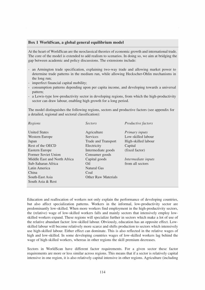
114
Box 1 WorldScan, a global general equilibrium model
At the heart of WorldScan are the neoclassical theories of economic growth and international trade.The core of the model is extended to add realism to scenarios. In doing so, we aim at bridging thegap between academic and policy discussions. The extensions include:
- an Armington trade specification, explaining two-way trade and allowing market power todetermine trade patterns in the medium run, while allowing Heckscher-Ohlin mechanisms inthe long run;
- imperfect financial capital mobility;- consumption patterns depending upon per capita income, and developing towards a universal
pattern;- a Lewis-type low-productivity sector in developing regions, from which the high-productivity
sector can draw labour, enabling high growth for a long period.
The model distinguishes the following regions, sectors and productive factors (see appendix for a detailed, regional and sectoral classification):
Regions Sectors Productive factors
United States Agriculture Primary inputsWestern Europe Services Low-skilled labourJapan Trade and Transport High-skilled labourRest of the OECD Electricity CapitalEastern Europe Intermediate goods (fixed factor)Former Soviet Union Consumer goodsMiddle East and North Africa Capital goods Intermediate inputsSub-Saharan Africa Oil from all sectorsLatin America Natural GasChina CoalSouth-East Asia Other Raw MaterialsSouth Asia & Rest
Education and reallocation of workers not only explain the performance of developing countries,but also affect specialization patterns. Workers in the informal, low-productivity sector arepredominantly low-skilled. When more workers find employment in the high-productivity sectors,the (relative) wage of low-skilled workers falls and mainly sectors that intensively employ low-skilled workers expand. These regions will specialize further in sectors which make a lot of use ofthe relative abundant factor: low-skilled labour. Obviously, education has an opposite effect. Low-skilled labour will become relatively more scarce and shifts production to sectors which intensivelyuse high-skilled labour. Either effect can dominate. This is also reflected in the relative wages ofhigh and low-skilled. In some developing countries wages of low-skilled workers lag behind thewage of high-skilled workers, whereas in other regions the skill premium decreases.
Sectors in WorldScan have different factor requirements. For a given sector these factorrequirements are more or less similar across regions. This means that if a sector is relatively capitalintensive in one region, it is also relatively capital intensive in other regions. Agriculture (including

food processing) and Consumer Goods employ relatively few high-skilled workers, whereas CapitalGoods, Electricity, Trade and Transport and Services (including the government) absorb many high-skilled workers. Sectoral restructuring can easily be linked to changes in relative endowments andchanges in (region-specific) demand patterns. This also holds because in WorldScan substitutionelasticities between domestic and foreign goods are believed to be high in the long run, at least muchhigher than in the short run. In principle, all goos are tradable, although trade in services is muchlower than in manufacturing and raw materials.
Except for different factor inputs, sectors vary also is some other respects. The sectors CapitalGoods and Services are the suppliers of investment goods and the sectors, Oil, Coal, Gas and otherRaw Materials only produce intermediate outputs. Consumer demand for electricity also includesdemand for other energy carriers. This assumption is made because nearly all demand for Rawmaterials is intermediate demand.
DataWorldScan has been calibrated on the GTAP database, see Mc Dougall et all. (1998). The calibrationyear is 1995. From this data base we derive not only demand, production and trade patterns, but alsolabour and capital intensity of the various sectors. The sectoral classification according to skillintensity is broadly correct, but the precise differences could very well change, when better databecome available.
The data and projections for population size and labour supply are from various sources. The UnitedNations (1995) provide demographic projections. The ILO (1996) provides projection rates onparticipation rates until 2010. We extrapolate the regional trends in participation rates between 1950and 2010 to 2020. The data for the supply of low-skilled and high-skilled workers at a regional levelhave been taken from Ahuja and Filmer (1995). Workers are labelled high-skilled when they havecompleted secondary education or a higher level. Ahuja and Filmer provide projections for manydeveloping countries. We lack projections for the OECD, Eastern Europe and the Former SovietUnion. Therefore we use the Barro and Lee (1996) data on education. We derive a trend betweenOECD and non-OECD regions between 1960 and 1990 and extrapolate this trend until 2020. Thedata on the size of the informal sector are obtained from the WorldBank (1995) and the ILO (1998).The IEA (1997) provides data on energy volumes and emissions in the base year 1995.
Substitution elasticitiesThe results of the model depend also on the substitution possibilities in production andconsumption. The production possibilities are described by a nested CES function. The upper leveldistinguishes between value added and intermediate goods. The elasticity between these two broadcategories is 0.4. At the lower level value added is described by Cobb-Douglas function of theprimary productive factors: capital, low-skilled labour and high-skilled labour. The intermediategoods are described by a nested CES function with a substitution elasticity of 0.8, which aggregatesEnergy and Other intermediates . The energy nest is a CES function which includes Oil, Petrol,Natural Gas, Electricity, but also Biofuels and Non-thermal electricity. The substitution elasticitybetween these inputs is 2.0. The second nest is also a CES function with again a substitutionelasticity of 0.8, which includes the other intermediate inputs.13 The utility function, from whichdemand for different consumption categories is derived, has been given a Cobb-Douglasspecification. The substitution elasticity between any pair of consumption categories therefore isunity.
115
Kyoto and Carbon Leakage
13 In case of the sector Electricity, the input Electricity is a part of the nest with other Intermediate inputs instead of the nest consistingof Energy.

Traded, foreign goods are not perfect substitutes for domestic goods, and this also affects theoutcome of simulations. The substitution between goods from different origin is not perfect.WorldScan employs an Armington-type assumption. However, the price elasticities of demandconsiderably increase over time. The model employs different assumptions for raw materials,Agriculture, Manufacturing and Services. The long-run substitution elasticities in the benchmarkcase are 17, 13, 7 and 5, respectively.
116
Johannes Bollen, Ton Manders and Hans Timmer
References
Bollen, J, A. Gielen, and H. Timmer (1999), Clubs,Ceilings and CDM, Macroeconomics of Compliance with the Kyoto Protocol, CPB NetherlandsBureau for Economic Policy Analysis, The Hague.
Lejour, A. (1999, forthcoming), The Interplay betweenGlobalization and Environmental Objectives, CPBNetherlands Bureau for Economic Policy Analysis.
McKibbin, W., R. Shackleton, and P. Wilcoxen (1998), ThePotential Effects of International Carbon EmissionsPermit trading Under the Kyoto Protocol, EconomicModelling of Climate Change, OECD Workshop Report.
Mensbrugghe, D. van der (1998), A (Preliminary) Analysisof the Kyoto protocol: Using the OECD GREENModel, Economic Modelling of Climate Change, OECDWorkshop Report.
Oliveira-Martins, J.M. Burniaux, and J.P. Martin (1992),Trade and the effectiveness of unilateral CO2-abatementpolicies: Evidence from Green, OECD EconomicStudies No. 19, Winter 1992.
Tang, P, R de Mooij, and R. Nahuis (1998), An economicevaluation of alternative approaches for limiting thecosts of unilateral regional action to slow down globalclimate change, European Economy No. 1.
WorldScan: the CORE model (1999, forthcoming), CPBNetherlands Bureau for Economic Policy Analysis,The Hague.
OECD (1997), The World in 2020: Towards a new globalage, Paris.
RIVM (1999, forthcoming), IMAGE-implementation of theB1 scenario - a greenhouse-gas emissions scenariodeveloped in support of the IPCC

Clean Development Mechanism: Discussion1
Robert A. McDougall
Owing to circumstances beyond my control, my remarks this afternoon will not be especiallyresponsive to Professor Heller’s. Also, while I have been involved in energy policy modeling forsome years, I cannot claim any particular expertise on the clean development mechanism (CDM).My remarks then will represent an outside observer’s perspective on the CDM debate. As an outsideobserver of the debate, I am struck by the high hopes placed on the CDM by some of its proponents.Contrary to those, it seems to me rather obvious that the CDM will play only a modest role in bothclimate change and sustainable development action. In my estimation, the CDM:
- is likely to prove contentious, - will lead to disappointment,- may yield some minor but useful reductions in the cost of abatement, but- will do little to assist development.
These outcomes do not re ect design weaknesses in the CDM, but are inherent in the basic concept.
The CDM is essentially a proposal for acting out of natural sequence. Developing countries are toparticipate before undertaking abatement commitments or implementing emission monitoringsystems. Industrialised countries are to participate in advance of therst commitment period, andwithout knowing the money value of the certied emission reductions their efforts procure. And thesystem is to come into operation in the year 2000, too soon for the rules to be well defined, or forthe necessary institutional machinery to be put in place.
To say this is not to criticize the CDM but merely to characterize it. The CDM aims at certainobjectives|early participation by developing countries, capture of early opportunities for cost-effective abatement action in those countries that would not otherwise be achieved. In pursuingthem, it is reasonable to make compromises in administrative tidiness and elegant design. Its out-of-sequence character does not make the CDM a bad nitiative, but an aggressive one, pushing theenvelope in terms of what is institutionally feasible. But this aggressiveness has implications for thelikely drawbacks and benefits of CDM action.
There are several ways in which the CDM may prove contentious.- Observers in developing countries have already expressed concern about the capacity of host
governments effectively to negotiate CDM contracts, the risk of early sell-off of low costabatement options, and the possibility of interference in host countries’ internal affairs (see forexample Zhang, 1999).
- The CDM does not attempt to increase global emissions abatement, but only to reduce the globalcost of abatement. Environmentalists are already unenthusiastic about mechanisms for vicariousfulfilment of industrialised countries’ commitments.
117
Clean Development Mechanism: Discussion
1 Full paper by Professor T. Heller has not been received.

They will be further disaffected if the CDM acts as a source of hot air. This it is liable to do, sincethe CDM operates under conditions where additionality is hard to verify, and since investors andhost countries have a common interest in colluding to overstate emission reductions.
- If stringent mechanisms are put in place to ensure that additionality is genuine, they will likely beresented by potential investors and by industrialised countries hoping to use the CDM to ease theburden of their Kyoto commitments.
- Most fundamentally, the CDM is the product of two different agendas, the sustainabledevelopment agenda of the developing countries, and a cost minimization agenda by someindustrialised countries. The CDM specification accommodates both sides’ aspirations, in thesense that it leaves room for both sides’ aspirations to be fulfilled. But that does not mean that bothsides’ aspirations will be satisfied by the actionthat in fact takes place under the CDM. In fact, thatseems rather unlikely, since large gaps remain in the two sides’ views on the role of theindustrialised countries in supporting sustainable development (see for example Ye, Jin, and Liu,1999). More than contentiousness however, the CDM is likely to lead to disappointment. Thereare several minor reasons why the extent of abatement action under the CDM is likely to be small.
- In the opinion of many observers, non-emission measures such as sequestration are excluded fromthe CDM.
- Effective safeguards to ensure additionality may impose burdensome delays and costs on would-be participants.
- Unlike other mechanisms, CDM projects are to be taxed, to meet administrative expenses and tofund unrelated adaptation projects.
But the major reason is that (assuming effective limitation of hot air) the incentive to participate inthe CDM is weak. The only formal incentive to participate is the certified emission reductionsprovided to investors. These are not usable until the first commitment period, which begins only in2008. The value they will bear at that time is unknown. Even the mechanism by which investorsmay use them is unknown. Until these uncertainties are resolved, the direct incentives to participatein the CDM will remain feeble.
Besides the direct financial incentives created by the CDM, there may also be indirect incentives.There may be some public relations benefits for investors or governments from 2 industrialisedcountries from participating in clean development projects. The CDM may encourage companies(like Shell) undertaking voluntary abatement on a global basis, to allocate more effort to projects indeveloping countries. The mere existence of the CDM as a topic of discussion may draw attentionto worthwhile potential projects in developing countries. While no doubt useful as far as they go,none of these indirect incentives seems likely to have more than a marginal impact on globalabatement or development. We are justified then in expecting that for some time to come, the levelof CDM action will be quite modest. Again, this does not mean that the CDM is ill-designed. It isbetter to do a little good than to do none at all. It means only that, given the difficulty of what isbeing attempted, too much should not be expected.
If CDM activity will be so modest, clearly its effectiveness in promoting development in the ThirdWorld will also be modest. Reinforcing this conclusion, we may note that the incentives for CDMaction depend only on the abatement potential, not the development potential, of the project. It hasbeen remarked that the word \development”, though it appears in the name of the CDM, is absent
118
Robert A. McDougall

from much discussion about the CDM, especially in a modelling context. In view of the nature ofthe incentives in the CDM, this omission appears realistic.
In summary, the CDM will achieve little cost reduction and little development, and is likely todisappoint many of the hopes placed in it. But realistically, if it achieves even a small amount ofcost reduction and a small amount of development, it will deserve to be considered a success.
119
Clean Development Mechanism: Discussion
References
T.C. Heller. Additionality, transactional barriers and thepolitical economy of climate change. Mimeo, 1997.
Ruqui Ye, Yunhui Jin, and Xue Liu. Analysis of advantagesand disadvantages of implementation of AIJ for China|apreliminary discussion. Paper presented at the IPCCWorking Group III Expert Meeting, 27-28 May 1999,the Hague, 1999.
ZhongXiang Zhang. Toward a sustainable development ofthe Chinese economy: Ac-complishments andchallenges in limiting greenhouse gas emissions. Paperpresented at the IPCC Working Group III ExpertMeeting, 27-28 May 1999, the Hague, 1999.

120

Discussion on the CDM1
Terry Barker
Three sets of comments are worth making in the debate on the effects of the CDM as a flexibleinstrument on the Kyoto Protocol.
The uncertainty of the size and scale of incremental abatement costs.
The CDM depends for its success on the identification and existence of large differences inincremental abatement costs between Annex B countries and non-Annex B countries and substantialmitigation schemes at these costs. However, it may be difficult to identify the costs and the schemes.There will be huge differences in costs depending on the technologies involved, the informationavailable, the incomes of those making the mitigation decisions, and the time available for theschemes to be planned and to operate. A usual assumption is that these incremental costs are lowerin developing countries, but this can be questioned. It seems likely that there is a huge range on costsin all economies and that there will be an overlap in the cost ranges between countries.
CDM effects as macroeconomic effects and environmental effects
If the CDM is to make a substantial contribution to GHG mitigation, through reducing the costs ofmitigation and/or increasing the level of mitigation, then it will have macroeconomic effects on theeconomies concerned. Although individual projects, programmes and schemes under the CDM maywell be assessed on a microeconomic cost-benefit methodology, when they accumulate to make anoverall contribution to mitigation they will affect the macroeconomy, and some of the underlyingassumptions of the original cost-benefit analyses will be changed.
This macroeconomic impact means that a macroeconomic analysis is necessary to assess the CDM.As such, a large number of mitigation studies have given net incremental benefits of mitigation, interms of effects on GDP and employment. Obviously the schemes with the largest net benefitsshould be taken first, ceteris paribus. There is also no indication from these studies that theincremental net benefits will reduce as time passes. Learning-by-doing and economics ofspecialisation and scale may well mean that the net benefits increase or the costs decrease. On theother hand if the revenues from the use of fiscal instruments eg carbon taxes are used to reduce onedistortionary tax after another, starting with the most distortionary, then as the taxes are removed,the net benefits should reduce.
121
Clean Development Mechanism: Discussion
1 Full paper by Professor P. Shukla has not been received.

Since there are likely to be environmental effects as well as economic effects of CDM schemes, egreductions is other emissions and damages associated with the reduction in GHG emissions, theseshould also be taken into account, further raising the social net benefits of CDM schemes.
Additionality and the CDM
There is a problem of additionality for all fiscal incentives, such as those associated with the CDM:how can participants be assured that the outcomes of a CDM scheme will indeed be additional tothose which would otherwise have occurred? In national incentive schemes, the problem isalleviated by requiring associated inputs or finance by those who receive the incentive.
In the case of a CDM project there are two sides to the additionality problem: i) how can the non-Annex B country be assured that the CDM funding will not replace other financial assistance? Andii) how can the Annex B country be assured that the mitigation will be additional? The problemshere can be alleviated by two requirements.i) A proportion of the funding for the CDM scheme (say 50%) should be available to the receiving
country for discretionary use.ii) Only 50% of the GHG savings be available to the Annex B country as a contribution to its Kyoto
mitigation requirements.
122
Terry Barker

Part III
Beyond Kyoto

124

Developing Economies, Capital Shortages and TransnationalCorporations (TNCs)
Leena Srivastava and Pradeep Dadhich
Developing economies and capital shortages
Poor countries and poor people differ from rich ones not only because they have less capitalbut because they have less knowledge (World Bank 1998/99). The scarcity of capital in developingcountries is a well-established fact reflected in the accumulated debt levels of these countries.Economic conditions suggested that borrowing money was a reasonable course of action in the1970s, particularly for poor countries, which perceived few, if any, alternative ways to address theeconomic plight of their citizens. The logic of borrowing is simple: one incurs a debt in the hope ofmaking an investment that will produce enough money both to pay off the debt and to generateeconomic growth that is self-sustaining. Unfortunately, the debt was not used either for developingresources nor for productive investments but more for financing current consumption (Ferraro andRosser 1994).
In 1970, the fifteen heavily indebted nations (using the World Bank classification of 1989) had anexternal public debt of $17.9 billion - which amounted to 9.8 percent of their GNP. By 1987, thesesame nations owed $402.2 billion, or 47.5 percent of their GNP. The most devastating effect of thisdebt burden is the significant outflows of capital to finance the debt. According to the World Bank(1989): “Before 1982 the highly indebted countries received about 2 percent of GNP a year inresources from abroad; since then they have transferred roughly 3 percent of GNP a year in theopposite direction.”
At around this time, the International Monetary Fund (IMF) emerged as the guarantor of thecreditworthiness of developing countries. The IMF approved additional loans to those countries thataccepted stabilization programs of “structural adjustment.” These programs are designed to addressbalance of payments problems that are largely internally generated by high inflation rates, largebudget deficits, or structural impediments to the efficient allocation of resources, such as tariffs orsubsidies. The IMF structural adjustment programs highlight “productive capacity as critical toeconomic performance” and emphasize “measures to raise the economy’s output potential and toincrease the flexibility of factor and goods markets.” They also assume that exposure tointernational competition in investment and trade can enhance the efficiency of local production andinvolve the relaxation of foreign exchange controls and privatisation of state enterprises. In a 1996article, Augustin Oyowe linked the increase in FDI flows to developing countries to the structuraladjustment programmes underway in these countries for almost ten years.
125
Developing Economies, Capital Shortages and Trans-national Corporations
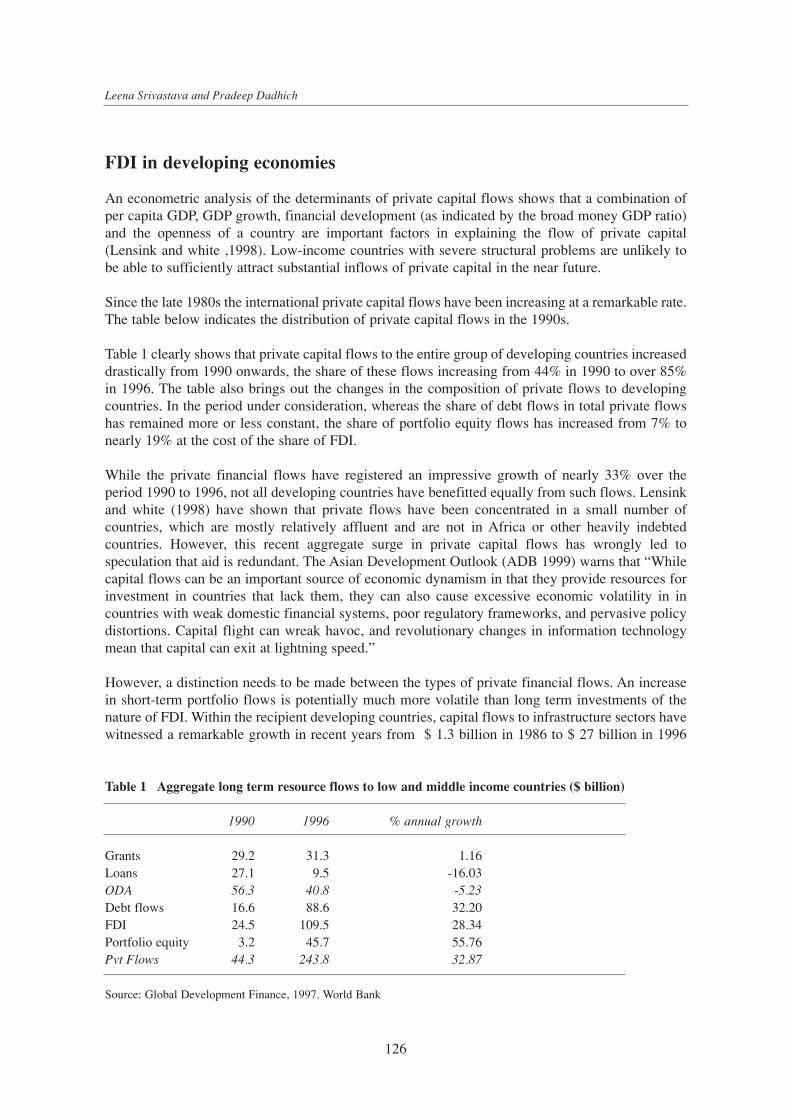
FDI in developing economies
An econometric analysis of the determinants of private capital flows shows that a combination ofper capita GDP, GDP growth, financial development (as indicated by the broad money GDP ratio)and the openness of a country are important factors in explaining the flow of private capital(Lensink and white ,1998). Low-income countries with severe structural problems are unlikely tobe able to sufficiently attract substantial inflows of private capital in the near future.
Since the late 1980s the international private capital flows have been increasing at a remarkable rate.The table below indicates the distribution of private capital flows in the 1990s.
Table 1 clearly shows that private capital flows to the entire group of developing countries increaseddrastically from 1990 onwards, the share of these flows increasing from 44% in 1990 to over 85%in 1996. The table also brings out the changes in the composition of private flows to developingcountries. In the period under consideration, whereas the share of debt flows in total private flowshas remained more or less constant, the share of portfolio equity flows has increased from 7% tonearly 19% at the cost of the share of FDI.
While the private financial flows have registered an impressive growth of nearly 33% over theperiod 1990 to 1996, not all developing countries have benefitted equally from such flows. Lensinkand white (1998) have shown that private flows have been concentrated in a small number ofcountries, which are mostly relatively affluent and are not in Africa or other heavily indebtedcountries. However, this recent aggregate surge in private capital flows has wrongly led tospeculation that aid is redundant. The Asian Development Outlook (ADB 1999) warns that “Whilecapital flows can be an important source of economic dynamism in that they provide resources forinvestment in countries that lack them, they can also cause excessive economic volatility in incountries with weak domestic financial systems, poor regulatory frameworks, and pervasive policydistortions. Capital flight can wreak havoc, and revolutionary changes in information technologymean that capital can exit at lightning speed.”
However, a distinction needs to be made between the types of private financial flows. An increasein short-term portfolio flows is potentially much more volatile than long term investments of thenature of FDI. Within the recipient developing countries, capital flows to infrastructure sectors havewitnessed a remarkable growth in recent years from $ 1.3 billion in 1986 to $ 27 billion in 1996
126
Leena Srivastava and Pradeep Dadhich
Table 1 Aggregate long term resource flows to low and middle income countries ($ billion)
1990 1996 % annual growth
Grants 29.2 31.3 1.16Loans 27.1 9.5 -16.03ODA 56.3 40.8 -5.23Debt flows 16.6 88.6 32.20FDI 24.5 109.5 28.34Portfolio equity 3.2 45.7 55.76Pvt Flows 44.3 243.8 32.87
Source: Global Development Finance, 1997. World Bank

(Dailami and Leipziger, 1998). Such flows embody certain desirable features, which bode well fortheir sustainability. In contrast to the short-term capital flows of the 1970s, flows to infrastructureprojects are of a long-term nature, with debt maturities of 7 to 15 years, or permanent equity and areinvested in assets which underpin long term economic growth and export expansion.
This is reinforced by the statistics in table 2. While Sub Saharan Africa has registered an impressivegrowth of 84.4 % in net private capital flows in the period 1990 to 1996, the growth in FDI hasbeen a mere 19.3 %. The statistics for Middle East and North Africa tell a similar story and boththese groupings of countries would probably feel insecure about their financial positions. On theother hand, Europe and Central Asian region has experienced a much higher growth in FDI ascompared to the aggregate net private flows.
Most FDI are based on activities undertaken by multinational corporations, but foreign investors areplaying an increasing role in privatisation projects in developing countries. “FDI involves theacquisition of existing businesses or development of new business enterprises in a foreign countrywith the intent of managing these businesses.” (ADB, 1999) Whereas, during the 1980s most FDIflows were between the countries of the North, by 1996 40% of new FDI flows from the North wereheaded towards the South (DeMartino, 1998).
Whereas, the attractiveness of FDI for developing countries is obvious in a situation of decliningofficial development finance share in total financial resource flows down to 14% in 1996compared to 56% in 1990, the attractiveness for FDI by investor countries, both in developed anddeveloping regions lies elsewhere. “Broadly speaking, FDI takes place to exploit an abundance ofnatural resources, use a relatively low-wage economy as a base for exports of labour-intensiveproducts, and circumvent trade barriers that limit the direct importation of products.” (ADB, 1999)
The role of TNCs
The increasing reliance on Foreign Direct Investment, and the continued wooing of the same bydeveloping countries through the spiralling move towards restructuring and reforming domesticeconomies, has propelled the TNCs into a major economic force unrestricted by geographicalborders. The 1995 World Investment Report indicated that 40,000 TNCs and their 250,000 foreign
127
Developing Economies, Capital Shortages and Trans-national Corporations
Table 2 Private capital flows to low and middle income countries ($ billion)
Net private capital flows Foreign Direct Investments1990 1996 % growth 1990 1996 % growth
Sub Saharan Africa 0.3 11.8 84.4 0.9 2.6 19.3East Asia and the Pacific 19.3 108.7 33.4 10.2 61.1 34.8South Asia 2.2 10.7 30.2 0.5 2.6 31.6Europe and Central Asia 9.5 31.2 21.9 2.1 15 38.8Latin America and the Caribbean 12.5 74.3 34.6 8.1 25.9 21.4Middle East and North Africa 0.6 6.9 50.2 2.8 2.2 -3.9All Countries 44.4 243.8 32.8 24.5 109.5 28.3
Source: Compiled from Global Development Finance, 1997 and the World Bank Debtor Reporting System

affiliates have sales in excess of US$ 5.2 trillion. The same report of 1998, indicates that in 1997some 53,000 TNCs and their 450,000 foreign affiliates accounted for a global sales valued at $ 9.5trillion and for $3.5 trillion as measured by the accumulated stock of FDI. Other performanceindicators, when looked at in relation to global performance are also very impressive. The ratio ofinward plus outward FDI stocks to global GDP in 1997 was 21%, value added by foreign affiliateamounts to 7% of global GDP and their exports account for one-third of world exports!
Undoubtedly, TNCs and the FDI that they bring in is of great importance to the developingcountries. This importance has been reinforced by the declining levels of overseas developmentassistance provided by the OECD countries. As seen in Table 1, during the period 1990 to 1996,ODA declined at an annual rate of a little over 5%. The ODA comprises on average a contributionof around 0.35% of a donor’s GNP (UNDP 1992), which compares poorly with the 25% of GNPthat the industrialised nations direct to their poor. Amongst the various modes of private financialflows, FDI is relatively attractive for the reasons often quoted:• provides access to modern technological and management knowhow• provides investment and employment opportunities• capacity building and training
That said, it needs to be recognised that there still exists a considerable amount of unease about therole of TNCs in developing countries in particular. Some of these concerns are listed in thefollowing section. This feeling of unease has also been reinforced by what is seen to be a victory ofvested interests in scuttling the efforts to institutionalise an international regulatory mechanism forTNCs. “The regulatory situation relating to Transnational Corporations (TNCs) and business ingeneral has worsened greatly in the past five years. The efforts to finalize a code of conduct onTNCs were formally killed in 1993, and the agency in charge of the code, the UN Centre onTransnational Corporations was closed. ... Instead, there has been a strong opposite trend nowdominant to reduce and remove more and more regulations that governments have overcorporations, to grant them increased rights and powers, while removing the authority of states toimpose controls over their behaviour and operations. The Uruguay round has already granted farhigher standards of intellectual property rights protection to the TNCs, facilitating further theirmonopolization of technology and their ability to earn huge rents through higher prices. ... Theability of governments to regulate the operations and effects of TNCs and companies in general isbeing severely curtailed.” (Khor, 1997)
TNCs: In conflict with developing country interests?
Profit maximising behaviour; little support to host countries’ economic and social developmentobjectives
Most TNCs perceive the Developing Countries as high-risk investments; especially the new andinexperienced TNCs. FDI coming from such TNCs are associated with high capital costs. TheseTNCs would like to recoup all their capital within 5-7 years and off load the equity at the end of ashort period of about 5 years. Because of the high capitalization rates, the market value of the capitalstocks increases significantly. The TNCs make a huge profit not only from the business operationsbut also from off-loading the equity holding. This leaves the company in the host country with littlecapital and poor managerial ability. Unless the company is managed extremely thereafter it willgenerally tend to become a sick company within the next 5-10 years time. This form of investmentgenerally lacks long term vision of social and economic welfare of the community.
128
Leena Srivastava and Pradeep Dadhich
Patented products and processes
The issue of intellectual property rights (IPRs) and patents has emerged as a major concern in theprocess of globalisation. Patents safeguard the results of a company’s research but the associatedpatents and licensing fees can be considered to be very expensive particularly by developingcountries. In the instances where FDI flows involve a transfer of technology, the potential forconflicts increases because developing countries may prefer the lower priced, albeit possibly less-efficient, technology alternatives.
Additionally, IPR issues are complex and distinctions as to what actually constitutes an IPR is notquite clear especially in the minds of persons involved in the technology transfer in the DC. Anexcellent example is a proposed AIJ project between a steel plant in India and an investing countryinvolving the installation of a scrap preheater and modification for continuous feeding of the scrapin an Electric Arc Furnace. In this case both the host country steel plant and the investor agreed thatthis could be treated as a case of technology transfer and this minor process modification would fallunder IPR. In fact, this technology is freely available within India but its capital intensity is themain reason for its low popularity among the mini steel plants.
Research Policy
Another area where interests of TNCs and developing countries do not necessarily assign the samepriorities relates to research. A TNC’s research policy and strategic direction are, understandably,geared towards furthering their own profit objectives and are determined by the global market ratherthan by national considerations. As such, the products and processes arising out of such efforts areagain not necessarily developed to meet local development priorities or adapted to local situations.
Transfer of technology by the TNC takes place through a licensing process, where the licensee cansell the technology to the user. In most cases there is a lag of about 5-7 years for the technology tobe transferred from the main technology generators to the licensees. The host country, in particularif it is a developing country, will have to wait over 10-14 years before they can receive such atechnological innovation. In the event that the host country seeks to obtain the technology directlyfrom the main TNC, the significantly high cost of the technology and the royalty charges wouldbecome a major barrier to the transfer of technology.
Location policy
This is another major area of contention between TNCs and national governments. Whilegovernments would like to see the maximum value addition taking place in-country and strive forself-sufficiency TNCs seek to locate production in the country which gives them the best investmentenvironment and market conditions.
The climate change problem, the Kyoto Protocol and the developing countries
The Framework Convention on Climate Change clearly recognised both historical responsibilitiesas well as the limited role that developing countries could play in addressing the problem of globalwarming. It called upon the developed (Annex 1) countries to stabilise their emission of GHGs to
129
Developing Economies, Capital Shortages and Trans-national Corporations

1990 levels by the year 2000 and move towards quantified emission limitation and reductioncommitments. It also called upon them to provide the requisite technologies and financial resourcesthat developing countries may need to do their bit, in line with their priorities, to contribute towardsthe objectives of the convention.The third meeting of the Conference of Parties (COP-3) at Kyoto adopted a Protocol to the FCCC,quantified the commitment levels of annex 1 countries and, at the same time, identified threemechanisms designed to provide flexibility to the Annex I Parties in order to meet theircommitments. These include:• Joint Implementation between Annex I Parties (though the term has not been explicitly used in
the text of the Protocol) (Article 6)• The Clean Development Mechanism (CDM) (Article 12)• Emissions Trading (Article 17)
Of these, the Clean Development Mechanism (CDM) holds promise of financial flows to thedeveloping countries, while the other two mechanisms may only influence the level and pattern offinancial resource flows.
The CDM defined in the Kyoto Protocol appears to be and is often perceived as a formalized JImechanism between developed and developing countries with credits. The benefits accruing fromCDM to the non-Annex I Parties would be the profits from project activities resulting in certifiedemissions reduction (CERs), while those to the Annex I Parties would be use of these CERs forachieving compliance with part of their quantified emission limitation and reductions.
The Climate change problem, developing countries and TNCs
Quite apart from the conflicts of interest noted in the sections above, several non-governmentalorganisations have been highlighting the role of TNCs in mitigating climate change. The ThirdWorld Network has been one of the most vocal institutions calling for a regulation of TNC activities.In their assessment, “TNC activities generate more than one half of the greenhouse gases emittedby industrial sectors with the greatest impact on global warming” (TWN 1997). In their assessmentgiven on the eve of the Earth Summit in 1992, “the biggest gap in the UNCED documents beingsigned in Rio is the absence of proposals for the international regulation or control of big businessesand transnational corporations to ensure that they reduce or stop activities that are harmful to theenvironment, health and development”.
Several issues relating to the climate change debate arise out of the role of TNCs in the globaleconomy. An attempt has been made in the following paragraphs to discuss the significant ones.
TNCs and emissions inventories
The business activities of TNCs are wide spread and diverse. Increasingly there is a complex globalscale integration in the production processes, while markets too are globally dispersed. Additionally,depending on the nature of investment, there could be a significant repatriation of profits back to thehome countries of the TNCs. All of this, combined with the fact that there is normally no long-term when seen in the context of the time frame of the climate change problem commitment of theTNCs to their host countries, makes the issue of accounting for green house gases from TNC
130
Leena Srivastava and Pradeep Dadhich
activities less than straight forward. A clear set of criteria would have to be identified on the basisof which emissions from TNC activities are budgeted. The criteria set would have to consider thenature of activities, the longevity of investments, the benefit sharing mechanisms, etc.
TNCs and the CDM
By the very nature of their business, TNCs are well positioned to take advantage of the Kyotomechanisms, in particular the CDM. As brought out by Casagrande (1996) over 70% ofinternational trade is controlled by TNCs. By 1989 trade between subsidiaries of TNCs accountedfor one-third of total world trade (DeMartino, 1998). The CDM mechanism envisages collaborativeproject-based activities between private companies in the developed countries and partnerorganizations in the developing countries. In return for flow of investments and technology, Annex1 partners would receive emissions reduction certificates presumably at costs much lower than ifthey were to bring about such reductions in their home countries. Obviously, the structure of TNCsplaces them in a position where they can take maximum advantage of such an arrangement. CDMprojects developed between a TNC (or its subsidiary) in a developed country and its subsidiarylocated in a non-annex 1 country would ensure that technology upgradation and the benefitstherefrom would remain within the company while giving the TNC the pick of such opportunitiesat the least net cost. Given their increasing role and influence in the developing countries, one fearcould be that, the negotiating position of the developing countries could be compromised.
While there is no international agreement yet on accrediting projects undertaken on a unilateralbasis or on projects based on opportunities for South-South cooperation, several studies havespoken about the contribution that such projects could make to the climate change agenda(Srivastava and Pathak, 1998). TNCs would be well poised to take advantages of such opportunitieswhich might arise in the future. Additionally, if these options are considered, TNCs can play a majorrole in influencing the trade in, and hence the prices of, CERs.
Apart from the monopolistic advantage of TNCs arising out of such a mechanism, several otherissues come to the fore. Most prominent amongst them is the issue of baselines. The question thatstares us in the face is whether the baselines for TNC projects should be the one for the host country,or should these be compared with the baselines in their home countries. Presuming that homecountry emission norms are much more stringent, a baseline based on the host country situationwould give a higher advantage to TNCs and may actually act as a disincentive for transfer of bettertechnologies and know-how. Yet another issue that is confounding is whether CDM activitiesbetween affiliates could be considered to be a leakage of benefits from the developing countries.This fear would arise from the cozy relationship between TNCs and their affiliates in developingcountries that would place the worldwide business interest of the TNC above the developmentpriority of the host country.
TNCs and emissions trading
The author considers the possibility of trading in hot air to be a carbon leakage. This considerationarises from the belief that only those emission reductions would qualify for trading which arise froma conscious effort to reduce such emissions. Reduced emissions arising from an economic slowdown or recession cannot, and should not, be traded. The implication of this argument is that:1. While the countries that are undergoing economic recession would, hopefully, bounce back over
a period of time, in the meanwhile they may be so strapped for investment resources as to lendthemselves to be exploited. Even if such hot air was to be utilised, it should be used to generate
131
Developing Economies, Capital Shortages and Trans-national Corporations
CERs or ERUs that reflect a tangible benefit to such countries at costs comparable to those insimilar projects in other countries.
2. Every unit of emission reduction should reasonably be able to be linked to specific policies ormeasures adopted or project activities. If such a system is allowed, then emissions trading wouldbe limited, primarily, to certified emission reduction units arising from JI projects and to certifiedemissions reduction arising from CDM projects. While TNCs would again be a majorbeneficiary of this development, it needs to be recognised that they can contribute to a significantdistortion in the emissions trading market.
Role of TNCs in climate change By virtue of their advantageous position vis-à-vis the CDM and JI mechanisms, TNCs can emergeas a major player in the emissions trading marketed. As mentioned by DeMartino “governments arefinding their policy autonomy constrained by the need to provide an environment conducive to theinterests of capital”. This is reinforced by Khor who says that “The ability of Governments toregulate the operations and effects of TNCs ... is being severely curtailed.” Given such a situationanother issue for consideration is whether TNCs should be considered as a ‘Party’ under theFramework Convention on Climate Change and the Kyoto Protocol. In such a scenario, whatentitlement would the TNCs have? And, at the same time, the issue arises on whether such anarrangement would further strengthen TNCs by placing them on the same level as the State?
In sum
This meeting addressed itself to the issue of the architecture of future agreements. Looking into thefuture, one sees two options:(i) The Kyoto protocol is ratified(ii) The Kyoto protocol is not ratified
If the Kyoto protocol is ratified, then the suggestions that follow should be kept in mind for theagreement that would be arrived at for the period beyond the Kyoto agreement. However, if theKyoto protocol is not ratified, the climate change community should address the roles andresponsibilities of TNCs explicity as soon as possible. The architecture of a future agreementshould: • need to work out a basis for equitable allocation of emissions entitlements• need to recognise the artificiality of divisions between the three Kyoto mechanisms• explicitly address the issues arising out of the growing power and reach of TNCs• consider appropriate governance/regulatory mechanisms.
132
Leena Srivastava and Pradeep Dadhich

References
ADB 1999. Asian Development Outlook, AsianDevelopment Bank
Casagrande Eloy F. 1996. Sustainable development in thenew economic (dis)order: the relationship between freetrade, transnational corporations, international financialinstitutions and ‘economic miracles’. SustainableDevelopment. Vol.4, 121-129.
Dailami M and Leipziger D. 1998. Infrastructure ProjectFinance and Capital Flows: A New Perspective. WorldDevelopment. Vol.26, No.7, pp. 1283-1298.
DeMartino George 1998. Foreign Direct Investment.Foreign Policy in Focus, Volume 3 No. 14, May 1998
FCCC Secretariat 1997 (Reprint). Framework Conventionon Climate Change. Bonn, Germany
FCCC Secretariat 1998. The Kyoto Protocol to theConvention on Climate Change. Bonn, Germany
Ferraro Vincent and Rosser Melissa 1994. Global Debt andThird World Development. From: World Security:Challenges for a New Century, edited by MichaelKlare and Daniel Thomas (New York: St. Martin’s Press,1994), pp. 332-355
Khor Martin 1997. Is globalisation undermining theprospects for sustainable development?. Fifth AnnualHopper Lecture, University of Guelph, October 21,1997.
Lensink R. and White1998. Does the revival ofInternational private capital flows mean the end of aid?An analysis of developing countries’ access to privatecapital. World Development, Vol.26, No.7. pp 1221-1234.
Oyowe Augustin 1996. Implications for developingcountries of liberalised financial services. The CourierACP-EU, No. 156, March-April 1996
Ritchie M. 1996.Control of Trade by Multinationals:impact of the Uruguay Round of GATT on sustainablefood security. Journal of the Society for InternationalDevelopment. Vol.4., 1996.
Srivastava Leena and Pathak Milind 1998. Kyoto Protocoland its Mechanisms. Tata Energy Research Institute,New Delhi 1998.
TWN 1997, TNCs and globalisation: Prime sources ofworsening ecological crisis. Third World Report No81/82, May/June 1997.
UNDP 1992, Human Development Report, United NationsDevelopment Programme
United Nations Framework Convention on ClimateChange. 1997. Trends of financial flows and terms andconditions employed by multilateral lending institutions.
World Bank 1989. World Development ReportWorld Bank. 1997. Global Development Finance. World
Bank, Washington, DC.World Bank 1998/99. “Knowledge for Development”
World Development ReportUNCTAD 1998. World Investment Report 1995. United
Nations Committee on Trade and Development, GenevaUNCTAD 1998. World Investment Report 1998: Trends
and Determinants. United Nations Committee on Tradeand Development, Geneva
133
Developing Economies, Capital Shortages and Trans-national Corporations

134

Future Agreements
James Edmonds1
The Framework Convention
The Framework Convention on Climate Change (FCCC) entered into force in 1994. It currently hasmore than 179 parties.2 This agreement forms the foundation for current international negotiationson climate change. Its goal is set forth in Article 2:
The ultimate objective of this Convention and any related legal instruments that the Conference ofthe Parties may adopt is to achieve, in accordance with the relevant provisions of the Convention,stabilization of greenhouse gas concentrations in the atmosphere at a level that would preventdangerous anthropogenic interference with the climate system. Such a level should be achievedwithin a time-frame sufficient to allow ecosystems to adapt naturally to climate change, to ensurethat food production is not threatened and to enable economic development to proceed in asustainable manner. (Emphasis added.)
The FCCC divides the world into three sets of nations Annex I, Annex II and non-Annex I. AnnexI nations are the developed nations of the world plus most of the Former Soviet Union and EasternEuropean nations.3 Annex II is a subset of Annex I, which excluding Former Soviet Union andEastern Europe, lists potential providers of financial assistance to developing nations.4
Annex I nations have greater responsibilities under the FCCC than non-Annex I nations. Thedistinction reflects concerns for differences in ability to participate by non-Annex I nations relativeto Annex I nations, as well as differences in historical rates of emission to the atmosphere ofgreenhouse gases. Annex I nations are to undertake measures with the “the aim of returningindividually or jointly to their 1990 levels these anthropogenic emissions of carbon dioxide andother greenhouse gases not controlled by the Montreal Protocol.” (Article 4)
In 1999 there appears to be little prospect for Annex I nations as a whole to achieve the aim of theFCCC—to return to 1990 emissions levels by the year 2000. In fact only a small number of nations
135
Future Agreements
1 This report was prepared as an account of work sponsored by an agency of the United States Government. Neither the United StatesGovernment nor any agency thereof, nor Battelle Memorial Institute, nor any of their employees, makes any warranty, express or implied,or assumes any legal liability or responsibility for the accuracy, completeness, or usefulness of any information, apparatus, product, orprocess disclosed, or represents that its use would not infringe privately owned rights. Reference herein to any specific commercialproduct, process, or service by trade name, trademark, manufacturer, or otherwise does not necessarily constitute or imply itsendorsement, recommendation, or favoring by the United States Government or any agency thereof, or Battelle Memorial Institute. Theviews and opinions of authors expressed herein do not necessarily state or reflect those of the United States Government or any agencythereof.
2 As of June 30, 1999.
3 Australia, Austria, Belarus, Belgium, Bulgaria, Canada, Czechoslovakia [sic], Denmark, European Economic Community, Estonia,Finland, France, Germany, Greece, Hungary, Iceland, Ireland, Italy, Japan, Latvia, Lithuania, Luxembourg, Netherlands, New Zealand,Norway, Poland, Portugal, Romania, Russian Federation, Spain, Sweden, Switzerland, Turkey, Ukraine, United Kingdom of Great Britainand Northern Ireland, and the United States.
4 Australia, Austria, Belgium, Canada, Denmark, European Economic Community, Finland, France, Germany, Greece, Iceland, Ireland,Italy, Japan, Luxembourg, Netherlands, New Zealand, Norway, Portugal, Spain, Sweden, Switzerland, Turkey, United Kingdom of GreatBritain and Northern Ireland, and the United States of America.
with special circumstances such as nations of the Former Soviet Union and Eastern Europe,Germany, and the United Kingdom, have much hope of returning greenhouse gas emissions to 1990levels by the year 2000.5
The Kyoto Protocol
From December 1 through December 11, 1997 participants in the FCCC met in the third Conferenceof the Parties held in Kyoto Japan to discuss measures that should be taken beyond those includedin the FCCC. An agreement was negotiated which established quantifiable emissions limitations forAnnex I parties, as well as a set of mechanisms to help reduce the cost of achieving the emissionslimitations including emissions trading, joint implementation, a Clean Development Mechanism(CDM), multiple greenhouse gases, and a five-year compliance period.
The Kyoto Protocol Has Not Entered Into ForceThe Protocol came open to ratification beginning March 16, 1999. It has not entered into force. Toenter into force, the protocol must be ratified by at least 55 Parties to the Convention, and ratifyingparties must represent at least 55 percent of the total Annex I carbon dioxide emissions for 1990.This means that if parties representing more than 45 percent of Annex I emissions remain outsidethe Protocol, it cannot enter into force. It is particularly important whether or not the United Statespresents an instrument of ratification, acceptance, approval or accession. It alone represents nearlyone-third of 1990 Annex I emissions.
For the United States, ratification of the Protocol requires a two-thirds vote of the Senate. It ispossible for the agreement to enter into force without the United States. However, without theUnited States participation it would require the absence of only a small number of additional nationsto make it impossible to achieve the 55 percent of 1990 emissions needed to enter into force.
Targets and TimetablesThe most prominent feature of the Kyoto Protocol is the quantified emissions limitations andreduction commitments. Thirty-nine parties accepted quantified emissions limitations or reductioncommitments. These are given in the Appendix to this paper.
We can summarize obligations as follows.• Western European nations accepted an eight percent reduction relative to 1990 emissions, with
the exception of Iceland and Norway which were allowed 110 and 101 percent of 1990 emissionsrespectively.
• Eastern European nations generally had the same obligation as Western European nations withsome exceptions—Croatia was 95 percent, and Hungary and Poland were 94 percent of base yearemissions. Note that the base year for the countries in this region need not be 1990.
• The Russian Federation and Ukraine were allowed 1990 emissions levels, while Latvia, Estoniaand Lithuania agreed to eight-percent reductions.
• Japan and Canada agreed to a six percent reduction from 1990 emissions levels.
136
James Edmonds
5 Restructuring and economic depression are the sources of the ability of Former Soviet Union and Eastern European nations to meettheir FCCC aim. For Germany, the reunification of East and West Germany in 1990 provided a base year with abnormally highemissions, which was followed by depression and restructuring in the East. In the United Kingdom, political measures against the coalminers’ unions and associated restructuring to natural gas make it possible to return to 1990 emissions in the year 2000.

• The United States of America agreed to reduce emissions seven percent below 1990 levels. And,
• Australia was allowed to increase emissions eight percent above 1990 levels and New Zealandwas allowed to emit up to 1990 levels.
The Six Gas ApproachEmissions are defined in terms of a basket of six gases: carbon dioxide (CO2), methane (CH4),nitrous oxide (N2O), hydrofluorocarbons (HFCs), perfluorocarbons (PFCs), and sulfur hexaflouride(SF6). Gases are compared to each other using global warming potential (GWP) coefficients asdeveloped by the IPCC. The use of GWPs allows for the aggregation of the six greenhouse gasesspecified in the Protocol into a singe value based on each gas’ carbon equivalent. We will discussthe use of carbon equivalent emissions in this analysis later in the paper.
Land-Use Change Emissions AccountingOne of the most important and controversial features of the Kyoto Protocol is the treatment ofemissions of greenhouse gases from land-use change. A very complicated set of rules wasdeveloped which addresses both political and scientific concerns. They describe how nationscompute their base year emissions, against which all future mitigation is measured, as well asemissions in the compliance years. The rules are complex, highly asymmetrical, and incomplete.6
137
Future Agreements
6 The Kyoto Protocol makes provision for land-use change emissions and sinks and, while net land-use emissions are small relative tofossil fuel carbon emissions, their treatment can have a major impact on the initial cost of achieving any emissions mitigation objective.Land-use emissions are presently treated as a flow in determining the base year (1990) emission rate. Most Annex I nations are in theprocess of reforesting, and therefore have net accumulation of carbon. This accumulation reduces net anthropogenic emissions.
Although this approach is appropriate for a global accounting of carbon flux, it may not be desirable as a methodology for setting 1990base year emissions. The implication of this treatment is that if a nation were reforesting in 1990 and were committed to maintaining1990 emissions rates under the Protocol, it could not reduce the rate of reforestation rate without lowering fossil fuel carbon emissionsto below 1990 levels. Thus reforesting is not enough. The rate must be maintained. For nations that were deforesting, this method wouldcreate a base year emission target that is the sum of deforestation plus fossil fuel emissions which would in turn implicitly grant thosenations a perpetual right to deforest. If the deforestation rate is ever reduced, for example as a consequence of destroying all forestedareas, then fossil fuel emissions could be higher than 1990 levels by the 1990 rate of deforestation.
The delegates at Kyoto agreed that if a country in the base year had net land-use accumulation of carbon—negative land-use changeemissions—the base year emissions for determining emissions limits would be determined by industrial emissions only. This methodwas termed the "gross" approach to accounting, a term which is anything but self-explanatory. The idea is that the country would noteits stock of terrestrial carbon, not the change in stock. In other words, land-use emissions are ignored in computing the base emissionsrate.
On the other hand, if a country were had net land-use carbon release, then it could count both industrial and land-use change emissionsin determining its base year emission inventory. This accounting method became known as the "net" approach.
In the budget period, 2008 to 2012, all countries include both industrial and net land-use emissions in their emissions inventory. For thosecountries with net emissions from land-use change in the base year, the accounting method was then the "net-net" approach in that netemissions flows are used in both the base year and the budget year. If a country has a net accumulation, however, it counts as negativeemissions only those accumulations of carbon that are the result of actions taken since 1990 in the areas of afforestation and reforestation.This method has come to be known as the "gross-net" approach in that net emissions are ignored in the base year but counted in the budgetperiod.
Many issues remain to be worked out. The protocol stipulates that
The net changes in greenhouse gas emissions from sources and removals by sinks resulting from direct human-induced land-usechange and forestry activities, limited to afforestation, reforestation, and deforestation since 1990, measured as verifiablechanges in stocks in each commitment period shall be used to meet the commitments in this Article of each Party included inAnnex I.
This presents an interesting problem in what to count. Do soils beneath the forests count? Can normal anthropogenic forest managementbe counted? Given the nature of forest growth, the rate of carbon uptake in 2008 would be small for a program that began in 1998 dueto the carbon absorption cycle by forests. Therefore, to the extent that net carbon uptake by sinks, or stores of carbon, is credited in thefirst budget period, it will largely be determined by an interaction between the rules and actions that were taken earlier. Unless interpretedvery broadly, the language of the Protocol limits the potential impact of new initiatives.

Emissions TradingThe principle of emissions trading was established in the Kyoto Protocol. However, severalimportant issues are left unresolved. Emissions trading could occur within or between Annex Iparties. Within a nation, domestic permit trading could take place among firms or other actors towhich permits are allocated. Similarly, permit trading could take place among firms or governmentsof different nations in an international permit market. Specific arrangements under which tradewould occur, however, are left to be worked out in the future. The Protocol also established theprinciple that, “trading shall be supplemental to domestic actions for the purpose of meetingquantified emission limitation and reduction.” Therefore, limits may be established in the use ofemissions trading to satisfy a commitment.
The Clean Development MechanismThe Protocol also established a Clean Development Mechanism (CDM). The CDM was created “toassist Parties not included in Annex I in achieving sustainable development and in contributing tothe ultimate objective of the Convention, and to assist Parties included in Annex I in achievingcompliance with their quantified emission limitation and reduction commitments under Article 3.”It allows emissions mitigation credits to be developed by non-Annex I parties beginning in the year2000, as long as these activities are supplemental to activities that would have been undertaken inthe normal course of events. It also identified a certification authority to insure that emissionsmitigation activities were in fact real and supplemental. As with emissions trading, the rules are leftto be developed in subsequent deliberations, and the degree to which this mechanism can captureemissions mitigation potential outside Annex I remains unclear.
ComplianceUnlike the Montreal Protocol, which established sanctions for non-compliance, the Kyoto Protocolestablishes no such penalties.
Agreements Beyond Kyoto
Even if it were to enter into force, the Kyoto Protocol could not be expected to achieve the goal ofthe FCCC. That is, it would not stabilize the concentration of greenhouse gases in the atmosphere,Figure 1.
The Protocol limits emissions controls to Annex B nations.7 We have calculated the concentrationof carbon dioxide in the atmosphere on the assumption that the Kyoto Protocol remains in forcebeyond the compliance period 2008 to 2012, throughout the remainder of the twenty-first century.We have assumed that there is no “leakage.” Leakage occurs whenever the emissions reductions ofone party are greater than global emissions reductions. Leakage can occur, for example, throughmarket interactions. Reductions in the demand for oil by mitigating nations can lead to lower oilprices which in turn could stimulate greater oil use in non-mitigating nations. Or, when mitigation
138
James Edmonds
7 This list is essentially the same as the list of Annex I nations. Annex B nations are: Australia, Austria, Belgium, Bulgaria, Canada,Croatia, Czech Republic, Denmark, Estonia, European Community, Finland, France, Germany, Greece, Hungary, Iceland, Ireland, Italy,Japan, Latvia, Liechtenstein, Lithuania, Luxembourg, Monaco, Netherlands, New Zealand, Norway, Poland, Portugal, Romania, RussianFederation, Slovakia, Slovenia, Spain, Sweden, Switzerland, Ukraine, United Kingdom of Great Britain and Northern Ireland, and theUnited States of America. This list varies somewhat from the countries contained in Annex I to the FCCC. Several countries such asSlovakia, Slovenia, Liechtenstein, and Monaco have been added, while Belarus and Turkey are listed in Annex I of the FCCC but notAnnex B of the Kyoto Protocol.
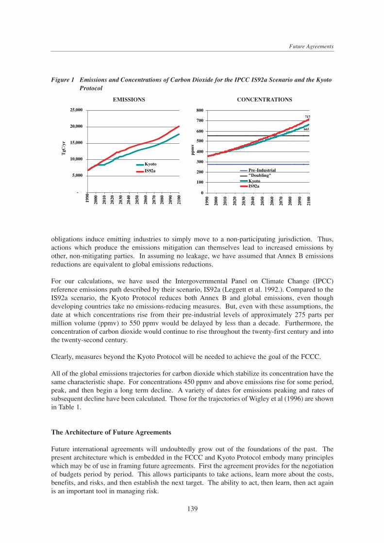
obligations induce emitting industries to simply move to a non-participating jurisdiction. Thus,actions which produce the emissions mitigation can themselves lead to increased emissions byother, non-mitigating parties. In assuming no leakage, we have assumed that Annex B emissionsreductions are equivalent to global emissions reductions.
For our calculations, we have used the Intergovernmental Panel on Climate Change (IPCC)reference emissions path described by their scenario, IS92a (Leggett et al. 1992.). Compared to theIS92a scenario, the Kyoto Protocol reduces both Annex B and global emissions, even thoughdeveloping countries take no emissions-reducing measures. But, even with these assumptions, thedate at which concentrations rise from their pre-industrial levels of approximately 275 parts permillion volume (ppmv) to 550 ppmv would be delayed by less than a decade. Furthermore, theconcentration of carbon dioxide would continue to rise throughout the twenty-first century and intothe twenty-second century.
Clearly, measures beyond the Kyoto Protocol will be needed to achieve the goal of the FCCC.
All of the global emissions trajectories for carbon dioxide which stabilize its concentration have thesame characteristic shape. For concentrations 450 ppmv and above emissions rise for some period,peak, and then begin a long term decline. A variety of dates for emissions peaking and rates ofsubsequent decline have been calculated. Those for the trajectories of Wigley et al (1996) are shownin Table 1.
The Architecture of Future Agreements
Future international agreements will undoubtedly grow out of the foundations of the past. Thepresent architecture which is embedded in the FCCC and Kyoto Protocol embody many principleswhich may be of use in framing future agreements. First the agreement provides for the negotiationof budgets period by period. This allows participants to take actions, learn more about the costs,benefits, and risks, and then establish the next target. The ability to act, then learn, then act againis an important tool in managing risk.
139
Future Agreements
-
5,000
10,000
15,000
20,000
25,000
1990
2000
2010
2020
2030
2040
2050
2060
2070
2080
2090
2100
TgC
/yr
Kyoto
IS92a
665
717
0
100
200
300
400
500
600
700
800
1990
2000
2010
2020
2030
2040
2050
2060
2070
2080
2090
2100
ppm
v
Pre-Industrial"Doubling"KyotoIS92a
Figure 1 Emissions and Concentrations of Carbon Dioxide for the IPCC IS92a Scenario and the Kyoto Protocol
EMISSIONS CONCENTRATIONS

Second, the present architecture utilizes recent experience as a reference in establishing limitationson future emissions. Unless future emissions constraints are grounded in near-term reality, there islittle hope that they can be achieved in practice.
Third, the present architecture provides for emissions trade between parties. Three institutionalmechanisms were incorporated: direct trade of emissions rights, joint implementation, and theCDM. The principle of “where” flexibility is an important tool in controlling the cost of emissionslimitation.
The principles that have been developed to date are, however, insufficient to achieve the objectivesof the FCCC. These principles must be expanded, and in doing so, they must deal with three criticalissues. They must:
• Address the long-term nature of the problem,• Provide mechanisms to control costs, and• Provide a mechanism to engage non-Annex I nations in the formal mitigation process.
Developing a Long-term Strategy
One of the most difficult features of the climate issue is the long-term nature of the problem. TheFCCC articulates the ultimate objective of the Convention in terms of concentrations—notemissions. This framing of the problem reflects the relationship between radiative forcing ofclimate change and the concentration of greenhouse gases in the atmosphere. Unlike conventionalpollution problems with which most negotiators are familiar, the relationship between emissions ofgreenhouse gases and their concentrations is complex. The removal mechanism for carbon dioxideinvolves non-linear, global, bio-geo-chemical processes.
Furthermore, significant uncertainty surrounds both the costs and benefits associated withalternative courses of action. Uncertainty is particularly acute with estimates of the benefits ofemissions mitigation. First, most of the beneficiaries are not yet alive. The consequences of climatechange that the present generation has any hope of significantly affecting lie many decades in the
140
James Edmonds
Table 1 The Relationship Between CO2 Concentration Ceilings, Maximum Emissions, and the Subsequent Rate of Emissions Decline: Wigley et al. (1996) Cases
Steady-State Concentration " 350 ppmv 450 ppmv 550 ppmv 650 ppmv 750 ppmv
Deflection Date IS92a a 2001 2007 2013 2018 2023Maximum Date 2005 2011 2033 2049 2062Maximum Emission b 6.0 8.0 9.7 11.4 12.5Rate of Decline e - 1.1% 0.8% 0.6% 0.5%
a The deflection date is the year in which emissions in the emissions stabilization trajectory first fall below IS92aemissions by more than 0.1 PgC/yr.
b PgC/yr fossil fuel carbon emissions on the date of maximum total anthropogenic carbon emissions.e Rate of decline in fossil fuel carbon emissions, in percent per year, over the first 75 years following the date of
maximum emissions. Note 350 ppmv not defined as it requires a negative net emission.

future. The present concentration of greenhouse gases has been largely determined by the actionsof preceding generations.
Second, for modest changes in the climate, estimates of costs and benefits disagree even about thesign of the damage. That is, some estimates show net benefits to the aggregate world economy fromsome additional net warming, though the benefits would not be evenly distributed around thesurface of the planet. See for example Mendelsohn et al. (1992, 1996) and Rosenberg (1993). Otherstudies show damages from even minor changes from present climate. See for example Cline(1993). Much of the net damage is associated with the valuation of unmanaged eco-systems, whichultimately disappear as rising surface temperatures push habitats to increasingly higher latitudes andaltitudes. Producing values for the prevention of species extinction is an extremely difficult andhighly uncertain enterprise. In addition to these problems of valuing the benefits to emissionsmitigation must be added the problem of surprises. As concentrations of greenhouse gases pushbeyond the bounds with which we have experience, the prospect that some unpleasant surprise maylurk unanticipated looms large.
The climate problem cannot be framed as a simple deterministic cost-benefit calculation. Rather, itmust be addressed as a risk management problem. Further, the primary focus must be on the risksassociated with alternative concentrations of greenhouse gases. This principle, like all goodguiding principles must be tempered by the realization that rates of change also matter.
As a consequence of the risk-based nature of the problem, policy decisions depend on the currentbest available information. Strategies that are developed to address the problem must deal with theneed to choose an initial concentration goal, based on the expected marginal benefits and marginalcosts of alternative concentrations. The quantitative goal established in this process is, of course,subject to change over time as knowledge accumulates.
The principle of “act, then learn, then act again” is an essential ingredient in the development offuture international agreement architectures. As noted earlier, this principle is already embodied inthe international agreement architecture developed within the FCCC and is embodied in Article 3.Interestingly, this is established within the context of the “precautionary principle.”
The Parties should take precautionary measures to anticipate, prevent or minimize the causesof climate change and mitigate its adverse effects. Where there are threats of serious orirreversible damage, lack of full scientific certainty should not be used as a reason forpostponing such measures, taking into account that policies and measures to deal with climatechange should be cost-effective so as to ensure global benefits at the lowest possible cost.
Controlling Costs
The largest obstacle facing the framers of future agreements is the control of compliance costs—also established as a principle in Article 3 of the FCCC. Without the development of a cost controlstrategy, no agreement, no matter how well conceived can persist. The control of greenhouse gasesis an altruistic enterprise. The present generation cannot affect the concentration of greenhousegases enough to alter the climate in which it will reside. The benefits to mitigation will be bestowednot on those alive today, but on their descendents.
Trade in emissions rights is a powerful tool for controlling the cost at any given period of time. Thegain from trade is one of the most fundamental results of economic science. A wide array of studies
141
Future Agreements

confirms this proposition. See for example, Weyant (1999), which confirms this finding for theKyoto Protocol. The principle of trade in mitigation obligations is established in the presentinternational architecture.
A second tool for controlling costs is to focus on the combined effect of all anthropogenic emissionsof greenhouse gases. While carbon dioxide is the most important greenhouse gas, it is not the onlyone. Methane, nitrous oxide, and a variety of manufactured chemicals also contribute significantlyto climate change. Framing emissions limitations in terms of a suite of greenhouse gases rather thanfocusing on each gas separately provides opportunities to deliver the same environmental benefitsat reduced cost. Again, this principle is embodied in the present international architecture.
The Hotelling/Peck & Wan Result
But other issues also need to be addressed. How much mitigation should be done and when loomsas the largest issue to be addressed by future agreements. The rate and timing of mitigation isgoverned by two factors—the basically cumulative relationship between emissions of carbondioxide and its atmospheric concentration, and the Hotelling/Peck & Wan theorems.
The Hotelling result (Hotelling, 1931) as modified by Peck and Wan (1996) states that the value ofa tonne of carbon should rise at the interest rate plus the rate of removal from the atmosphere. Thelogic of this result is simple. The right to emit carbon is a scarce resource that can be used toproduce goods and services. By virtue of the cumulative nature of the relationship betweenemissions and concentrations, a fixed concentration ceiling implies a fixed cumulative emissionover all time. This asset should behave like other economic assets. Those who hold onto the assetsshould be rewarded at the same rate as those who hold onto other financial assets. The value of atonne should appreciate at the same rate as other investment such as bonds.8 Peck and Wan (1996)showed that if carbon is removed from the atmosphere, the price must rise sufficiently faster thanthe interest rate to compensate those who hold emissions rights for the lost value from theirdisappearing asset.
The Hotelling/Peck & Wan result has important implications for framing future agreements. Itimplies that early costs should be low but rise steadily. There is a complementary physicalimplication of these results. Initial emissions mitigation should be modest, but the deviation fromreference should grow steadily. The incremental nature of these results is important and might besummarized as “small steps before large ones.” It allows for the orderly turn over of the capitalstock, the conduct of research and technology development, prevents lock-in to early version of newtechnologies which are rapidly improving, and allows time for new infrastructure to be developed.
Premature retirement of capital stock adds significantly to the cost of mitigation. Wheneverinvestments must be prematurely scrapped, remaining productivity is lost forever. It is this losswhich society feels. Premature retirement of capital is a problem which occurs at the beginning ofa policy intervention. Once a policy regime is established, investors can plan accordingly. It is theunanticipated nature of the policy intervention which raises the potential for losses from prematureretirement of capital. The gradual and incremental nature of the Hotelling/Peck & Wan principleminimizes such unanticipated losses.
142
James Edmonds
8 If the value of a tonne of carbon rises at a rate faster than the rate of interest, no one will hold bonds. Bond prices will fall, raising therate of interest and bringing the markets back into balance. The opposite occurs should the value of a tonne of carbon rise more slowlythan the rate of interest.

Technology and Cost
In the near term technology options are limited to those technologies which are currently available.In the long term technology can and will change. The path and rate of technology development willplay a large role in shaping the future cost of meeting an emissions limitation requirement.
Edmonds et al. (1999) explored carbon dioxide concentration stabilization scenarios. Thesescenarios employ the Hotelling/Peck & Wan approach to formulating intertemporal time paths ofemissions limitations. Such paths have modest initial emissions mitigation requirements but theserequirements grow with time. Figure 2 shows a reference emissions trajectory, an allowableemissions limit (gray) and carbon emissions reductions associated with the expansion of specificenergy technologies.
While the magnitude of change in the first half of the twenty-first century is modest, the eventualmagnitude of change in the reference case at the end of the twenty-first century is large.Technologies whose activity levels expand to provide the emissions mitigation include those forwhich no large scale deployment currently exists, for example, solar energy, carbon capture andsequestration from power systems, hydrogen production and power conversion from fuel cells, andcommercial biomass energy. Contemporary versions of all of these technologies exist. None,however, are deployed at scale. Since the infrastructure needed to deploy many of thesetechnologies does not currently exist, now only will it be necessary to develop the base technology,but it will also be necessary to simultaneously develop and deploy the supporting capitalinfrastructure.
Mitigation is not the only policy option. Investments in science and technology provide informationabout potential impacts—making better evaluations of appropriate risk management responsespossible. Investments in science and technology also provide the knowledge base needed todevelop new energy technologies.
143
Future Agreements
Figure 2 Global Carbon Emissions in a Reference Case, Emissions Limitations Associated with a 550 ppmv Concentration Ceiling, and Emissions Mitigation Associated with the Expansion of Various Energy Technologies Relative to the Reference Case.
1990 2005 2020 2035 20502065 2080
2095
0
5,000
10,000
15,000
20,000
25,000
Mill
ions
of
Ton
nes
of C
arbo
n pe
r ye
ar
soil carbon sequestrationsequestration from fossil power generationsequestration from synfuels productionsequestration from H2 productionend-use technology improvementsnuclearsolarbiomass550 ppmv emissions

Ultimately, investments in science and technology will be effective only if they are accompanied bypolicies which demonstrate a commitment to a transition to a world in which emissions arecontrolled.
Accession
One of the fundamental characteristics of the climate change problem is that greenhouse gases arewell mixed in the atmosphere. Thus, the geographical source of greenhouse gases is irrelevant. Itis the sum of all sources from all locations over long periods of them that determines theirconcentrations.
The FCCC accepted the principle of common but differentiated responsibilities and recognized aspecial responsibility for developed nations.
The Parties should protect the climate system for the benefit of present and future generationsof humankind, on the basis of equity and in accordance with their common but differentiatedresponsibilities and respective capabilities. Accordingly, the developed country Partiesshould take the lead in combating climate change and the adverse effects thereof. (UNFCCC, Preamble, emphasis added)
The FCCC charged Annex I nations the goal of returning to 1990 emissions levels by the year 2000.The Kyoto Protocol established quantifiable emissions limitations for Annex B nations. Non-AnnexI nations have no obligations. While the Kyoto Protocol establishes a Clean DevelopmentMechanism (CDM) to engage developing nations in emissions mitigation, the effectiveness of theCDM is limited by its lack of a clear quantified benchmark against which to measure emissionsmitigation and the fact that the Kyoto Protocol has not entered into force.
Emissions of Annex I nations are anticipated to be smaller than those of non-Annex I nationssometime before the year 2030. The IPCC IS92a scenario, for example estimates the crossing pointto occur in 2025, Figure 3.
144
James Edmonds
0
2
4
6
8
10
12
14
16
1990
2000
2010
2020
2030
2040
2050
2060
2070
2080
2090
2100
Year
Bil
lion
s of
Ton
nes
of C
arbo
n pe
r Y
ear
Non-Annex I
Annex I
Figure 3 IPCC IS92a Carbon Emissions by Annex I and Non-Annex I Nations

It is not difficult to show that there are insufficient emissions in Annex I nations to independentlystabilize the concentration of greenhouse gases (Edmonds, et al., 1997). Annex I emissionsmitigation alone would eventually be insufficient to stabilize the concentration of carbon dioxide,even if the stabilization ceiling is 750 ppmv (Table 2).
Ultimately Non-Annex I nations must take on obligations if the concentration of carbon emissionsis to be stabilized. This raises the question of accession. Accession is a highly sensitive questionas it raises issues of fairness, justice and equity. While all nations of the world have a stake incontrolling the emissions of greenhouse gases it is not the highest priority of developing countries.Development is the highest priority of the world’s poor nations.9 On a practical level, accession alsoraises questions about the institutional capacity of non-OECD governments to monitor and enforceobligations.
The present system of quantified emissions limitations established under the FCCC and KyotoProtocol, is founded on a principle of emission allocation that is based on historical emissions. Thisis sometimes referred to as a “grandfathered” emissions principle. That is, one has the right to emitin the future what one emitted in the past. This principle has been used in past allocations ofemissions rights in both domestic and international contexts and appears to have achieved the statusof the practical default principle. It is not the only possible basis for emissions allocations. Manyothers have been put forward. Other simple principles that could be used include basing emissionsallocations on the number of people in a nation, historical cumulative emissions, the scale ofeconomic activity (GDP), and fossil carbon resources.
In a trading regime in which emissions are capped and traded the emissions rights have economicvalue. The value of emissions rights is the product of allocated emissions and the value of a tonneof carbon. These values can be large. For example, for a 550 ppmv ceiling, the MiniCAM modelshows global allowable fossil fuel emissions can rise to one trillion dollars per year (1990 constantUS dollars, Edmonds et al., 1999). The allocation of emissions rights determines how this value isdistributed. Allocating emissions rights to all of the nations of the world on the basis of 1990emissions implies a large wealth transfer from developing nations to developed nations. It is notsurprising that developing country negotiators find grandfathered emissions unacceptable. Incontrast allocating emissions on the basis of population implies a large transfer of wealth from thedeveloped world to the developing nations.
145
Future Agreements
Table 2 Relationship Between Concentration Ceiling and Year in Which Annex I Emissions MitigationAlone Is Inadequate to Achieve Atmospheric Stabilization
Carbon Dioxide Concentration Ceiling " 450 ppmv 550 ppmv 650 ppmv 750 ppmv
Year in which Annex I emissions mitigation alone is insufficient to maintain global emissions on a path that would stabilize the concentration of 2035 2065 2085 2095atmospheric carbon dioxide, assuming IPCC IS92a emissions paths and no “leakage.”
9 Development may be one of the strongest climate change policy responses. Schelling (1997) has argued that developed nations are farbetter positioned to cope with the consequences of climate change, and that economic development is therefore a potentially importantelement of developing nations’ climate change response.

Large transfers of wealth to foreign nations can be a domestic political problem even if it occurs inthe context of a minimum cost mitigation regime (Victor, 1999). Part of the reason thatgrandfathered emissions has proved an attractive principle in emissions allocations amongdeveloped nations is that even in a cap-and-trade regime it implies relatively small near-term wealthtransfers among parties.10
The same transfer-of-wealth problems occur within any nation that allocates emissions rights withinthe context of a cap-and-trade regime.
Accession Strategies—Jacoby et al.
Several research groups have begun to think about developing burden-sharing rules to deal withconcerns for fairness and equity. Jacoby et al. (1998) explored a generalized approach based on“ability-to-pay” as a surrogate for “willingness to pay.”11 As the standard of living in a nation rises,the relative value of additional material goods declines relative to environmental services. Richernations are more willing to take on environmental burdens than poorer nations.
Jacoby et al (1998) demonstrate by example, that it is possible to construct a set of rules which willstabilize the concentration of carbon dioxide in the atmosphere and provide for a gradual transitionfrom non-participation to full participation. They created a, universal formula for emissionslimitations:
γ - a(wt-1 – w*)wreft-1 > w*
ηt = (dC/dt)/Ct = ηref
t otherwise
where C = carbon emissionsηt = rate of emissions change (+ or -) per yearw = a “trigger” defined in terms of some per-capita welfare measure, and
α and γ are parameters which determine the rate of change of burden with changein the welfare measure.
Three things are important about this formulation. First, below some per capita welfare thresholddefined by the “trigger” no limits are placed on the rate of growth of emissions. Second, once thethreshold is crossed there is a gradual transition from non-participation to full participation. Andthird, the formulation is general, applying to all participants. It is important to note that thisformulation defines an emissions limit for each period relative to its own base. It does not adopt anabsolute reference, for example 1990 emissions. Rather, the reference is continually being updatedwith time.
Using per capita income as the measure of welfare, Jacoby et al. demonstrated that stabilization ofthe concentration of greenhouse gases is possible. They note, however, that this approach does notattempt to create an inter-temporal, cost-effective trajectory to stabilization of concentrations. They
146
James Edmonds
10 Victor (1999) points out that one of the problems with the Kyoto Protocol is the disparity in obligations relative to present emissions.This disparity primarily affects the Former Soviet Union, which negotiated an emission allowance equivalent to its 1990 level, but whoseemissions have fallen dramatically as a consequence of economic restructuring. A wide array of economic analyses show that free tradein emission allowances among Annex I nations under the Kyoto Protocol implies a sizable transfer of wealth from OECD nations to theFormer Soviet Union (Energy Economics, 1999, special issue).
11 There is evidence that ability to pay is a reasonable surrogate for willingness to pay. See for example Grossman and Krueger (1995).

argue that while a century-scale cost minimization calculation is an interesting academic exercise,it is uninteresting in the real world. Within a budget period, however, costs are reduced when tradeamong parties is allowed.
Trade in emissions rights between participants within budget periods is shown to significantlyreduce costs (or increase benefits) to participants. By placing the greatest mitigation burden on therichest countries, which tend also to be the highest emitting countries (per capita), there would alsotend to be transfers of resources from the richer nations to poorer nations with trade in emissionsrights.
Accession Strategies—Edmonds and Wise
Edmonds and Wise (1999) have also examined alternative emissions mitigation agreementarchitectures. They demonstrated that an agreement focused on new investments and establishinggeneric performance standards and income-based accession could also stabilize the concentration ofcarbon dioxide in the atmosphere. Their approach is built on the observation that in modernsocieties carbon flows through two sectors—power generation and fuel refining and processing.They create a simple set of rules as follows:
In the first stage emissions from new capacity in powerplants and synfuel conversion facilities arecontrolled in OECD nations. After a fixed date new capacity must be carbon neutral, that is emitno net carbon. For synfuel conversion facilities this means that all carbon released in the upgradeof coal to liquids and gases must be captured and disposed of in an environmentally safe manner.New power generation facilities coming on line after the start-date can either use non-carbon fuelssuch as nuclear fission, fusion, solar, wind, biomass, or hydro, or they can utilize fossil fuels butcapture and sequester the carbon in an environmentally safe manner. Other parties to the agreementtake on the same obligations as OECD nations when their per capita income levels reach those ofthe lowest OECD nations taking on the initial obligation.12
The second phase would control refining and processing of fossil fuels. It would begin in the OECDand require new facilities to be carbon neutral after a fixed date. They could use fossil fuels as afeedstock for the production of hydrogen, but could not pass net carbon to the economy. Over thefollowing 45 year period net imports of carbon-based fuels would be phased out. Non-OECDnations would take on the same obligation as OECD nations when their per capita incomes rose tothat of the lowest OECD nation which undertook the initial obligation.
Edmonds and Wise examined a variety of cases. Starting the first phase in the year 2035 and thesecond phase in 2065 results in the stabilization of concentrations of carbon dioxide between 525and 550 ppmv. Earlier dates of first compliance are consistent with lower concentration ceilings,and later dates are consistent with higher concentration ceilings. Because of the focus on largefacilities monitoring and enforcement is made easier. In addition, no international transfers ofwealth need occur.
This strategy uses a general performance standard to drive the development and dissemination oftechnology. One can easily imagine the development of fuel cells to generate carbon-free power,which in turn would generate a demand for hydrogen and the transmission capacity to deliver it.
147
Future Agreements
12 To prevent manipulation of the income test, for example, through exchange rate policy, incomes would need to be measured in termsof a purchasing power parity index. The income test could be framed in terms of the date of agreement with a fixed "grace" period tofollow before new sources need comply

This in turn could result in improved hydrogen fuel cells, which could then be utilized in thetransportation sector, and the trunk lines which could become the foundation for a more generalhydrogen transmission system.
By focusing on activities which utilize large facilities, monitoring and compliance costs would bereduced. Focusing exclusively on new sources avoids the stranded asset problem.13 And, sinceobligations are domestic, no transfers of funds need occur.
The strategy, like the Jacoby et al. approach, does not minimize the present discounted cost ofstabilizing concentrations at a given level. Costs could be reduced by giving credit for early actionboth domestically and internationally.
Both the Jacoby et al. and Edmonds and Wise approaches explore long-term strategies which takeseriously the question of fairness and equity. They also show that there are potentially manyalternative approaches which build upon the foundations of the present international architecture toaddress climate change.
Summary
The current set of international agreements is based on the Framework Convention on ClimateChange (FCCC). The FCCC has as its ultimate objective the stabilization of concentrations ofgreenhouse gases at levels which would prevent dangerous anthropogenic interference with climatesystems. It establishes a variety of principles which should be utilized in the implementation of thisobjective, including cost effectiveness, fairness, and equity. Since the FCCC entered into force theparties have met on several occasions to discuss the adequacy of commitments. The 1997conference of the parties, meeting in Kyoto, drafted the Kyoto Protocol, which focuses on additionalcommitments to be undertaken during the time period 2008 to 2010.
Even if the Kyoto Protocol enters into force, further agreements will be needed to achieve the goalof the FCCC. These further agreements will have to confront three broad areas of concern:
• Extension of the reference time frame to a century,• Control of costs, and • Expansion of the list of nations with quantifiable emissions limitations.
The first issue could be productively addressed by framing the goals of international agreements interms of an explicit concentration objective for greenhouse gases, recasting the problem in terms ofrisk management, and broadening the set of tools for controlling emissions to include technologydevelopment and deployment.
Control of costs is essential, as mitigation, if it occurs, will be undertaken largely by those who willnot benefit from their own sacrifices. Tools for addressing this issue include trade in mitigationobligations, tradeoffs within a group of greenhouse gases, minimizing capital stock turnover, anddeveloping and deploying successive generations of mitigation technologies. The Hotelling/Peckand Wan theorems govern the relationship between the value of carbon in one period compared tothe next. These theorems require that the value of a tonne of carbon rise over time at the rate of
148
James Edmonds
13 To avoid indefinite life-extensions, it is necessary to define "lifetimes" for existing capacity, after which a facility is treated as a newsource.

interest plus the rate of removal of carbon from the atmosphere. Initial carbon values are thereforelow, requiring modest, but real, early mitigation, minimal premature loss of capital, and steadilyrising obligations. It also allows time to develop and deploy new technologies and preventspremature “lock-in” to immature versions of new technologies.
Future agreements must also expand membership in the group of parties with emissions mitigationobligations. Such an expansion will require addressing issues of fairness and equity. Twoarchitectures for accession are discussed. Both use per capita income as the criterion for accession.One sets national mitigation limitations explicitly. The other focuses on the character of newtechnologies. Either can stabilize concentrations of greenhouse gases.
Acknoledgements
I would like to express his appreciation to the United States Department of Energy and to EPRI forsupport made this work possible. I would also like thank the organizers of the IPCC Working GroupIII Expert Meeting held in Den Haag, May 27-28, 1999 for providing the motivation andopportunity to assemble the material found in this paper. I would also like to thank Henry Jacoby,who spent substantial amounts of time in consultation with me, and who provided many of the goodideas presented here. The author also benefited from conversations with Richard Richels and JohnWeyant. The author would also like to thank Ambassador Richard Benedick, Jim Dooley, RonSands, and Elizabeth Malone for comments on an earlier draft of the paper. While I am indebted tothem for their many insights, responsibility for any remaining errors or misinterpretations remainswith the author.
149
Future Agreements

References
Cline, W.R. 1992. The Economics of Global Warming.Institute for International Economics, Washington, DC.
Edmonds, J., Dooley, J., and S.H. Kim. 1999. “Long-termEnergy Technology: Needs and Opportunities forStabilizing Atmospheric CO2 Concentrations,” inClimate Change Policy: Practical Strategies toPromote Economic Growth and EnvironmentalQuality. Monograph series on tax, trade andenvironmental policies and U.S. economic growth,American Council for Capital Formation, Center forPolicy Research, Washington, DC. pp. 81-97.
Edmonds, J., and M. Wise. 1999. “Exploring ATechnology Strategy for Stabilizing Atmospheric CO2,”International Environmental Agreements on ClimateChange. Kluwer Academic Publishers. PP.131-154.
Edmonds, J., Wise, M. and Dooley, J. 1997. “AtmosphericStabilization and the Role of Energy Technology,” inClimate Change Policy, Risk Prioritization and U.S.Economic Growth, C.E. Walker, M.A. Bloomfield andM. Thorning (eds.). American Council for CapitalFormation, Washington DC. (pp71-94).
Grossman, G.M. and A.B. Krueger. 1995. “EconomicGrowth and the Environment,” Quarterly Journal ofEconomics. 110(2):353-377.
Hotelling, H.. 1931.. “The Economics of ExhaustibleResources”. Journal of Political Economy, 39, 137-175.
Jacoby, H.D., R. Schmalensee, and I.S. Wing. 1998.Toward a Useful Architecture for Climate ChangeNegotiations. Joint Program on the Science and Policyof Global Change, Massachusetts Institute ofTechnology, Cambridge, MA.
Leggett, J., W.J. Pepper, R.J. Swart, J. Edmonds, L.G.Meira Filho, I. Mintzer, M.X. Wang, and J. Wasson.1992. “Emissions Scenarios for the IPCC: An Update.”in Climate Change 1992: The Supplementary Reportto the IPCC Scientific Assessment, University Press,Cambridge, UK. Change.
Mendelsohn, R., R. Adams, J.M. Callaway, B. Hurd, B. McCarl, W. Morrison, K. Segerson, J. Smith, B.Sohngen, and G. Yohe. 1996. The Market Impacts ofClimate Change in the US. Paper presented to theInternational Workshop on Climate Change:Integrating Science, Economics and Policy, 19-20March 1996, IIASA, Laxenburg Austria. Yale School ofForestry and Environmental Studies, Yale University,New Haven, CT 06511, USA.
Mendelsohn, R., W.D. Nordhaus and D. Shaw. 1992. TheImpact of Climate on Agriculture: A RicardianApproach. Paper presented to the InternationalWorkshop on Costs, Impacts, and Possible Benefits ofCO2 Mitigation, 28-30 September 1992, IIASA,Laxenburg, Austria. Cowles Foundation for Research inEconomics at Yale University, Box 2125, YaleUniversity, New Haven, CT, USA.
Peck, S.C. and Y.H. Wan. 1996. “Analytic Solutions ofSimple Greenhouse Gas Emission Models,” Chapter 6 ofEconomics of Atmospheric Pollution, E.C. Van Ierlandand K. Gorka (eds.), Springer Verlag 1996
Rosenberg, N.J. (ed.) 1993. Towards an IntegratedImpact Assessment of Climate Change: The MINKStudy. Kluwer Academic Publishers, Boston.
Schelling, T.C. 1997. “The Costs of Combating GlobalWarming,” Foreign Affairs, 76(6):8-14.
United Nations. 1992. Framework Convention on ClimateChange. United Nations, New York.
United Nations. 1997. Kyoto Protocol To The UnitedNations Framework Convention On Climate Change.United Nations, New York.
Victor, D. 1999. Weyant, J. 1999. “Kyoto Protocol,” Energy Economics.
VV(nn):pp-pp.Wigley, T.M.L., R. Richels & J. A. Edmonds. 1996.
“Economic and Environmental Choices in theStabilization of Atmospheric CO2 Concentrations,”Nature. 379(6562):240-243.
150
James Edmonds
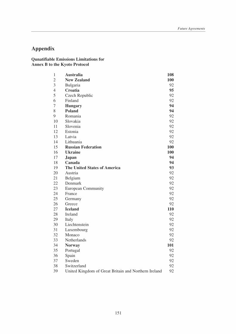
Appendix
Qunatifiable Emissions Limitations forAnnex B to the Kyoto Protocol
1 Australia 1082 New Zealand 1003 Bulgaria 924 Croatia 955 Czech Republic 926 Finland 927 Hungary 948 Poland 949 Romania 9210 Slovakia 9211 Slovenia 9212 Estonia 9213 Latvia 9214 Lithuania 9215 Russian Federation 10016 Ukraine 10017 Japan 9418 Canada 9419 The United States of America 9320 Austria 9221 Belgium 9222 Denmark 9223 European Community 9224 France 9225 Germany 9226 Greece 9227 Iceland 11028 Ireland 9229 Italy 9230 Liechtenstein 9231 Luxembourg 9232 Monaco 9233 Netherlands 9234 Norway 10135 Portugal 9236 Spain 9237 Sweden 9238 Switzerland 9239 United Kingdom of Great Britain and Northern Ireland 92
151
Future Agreements

152

Developing Country Effects of Kyoto-Type EmissionsRestrictions
Mustafa Babiker and Henry D. Jacoby*
1. The Issue of Burden Sharing
In a world without international trade, the costs of pollution control measures would be pretty wellconfined to the country taking the action. We live in a world tightly knit by trade, however,importantly including a massive trade in oil and other fossil fuels. Thus if restrictions on carbonemissions are adopted by a sub-set of nations, the effects will be felt throughout the world economy.In the countries accepting greenhouse restrictions the cost of using carbon-emitting fossil fuels willrise, simultaneously lowering the demand for these fuels (thereby reducing their internationalprices) and raising the cost of goods that require them as inputs. Also, the total level of economicactivity in these countries may fall somewhat relative to the output levels that otherwise would beachieved, lowering their demand for imports of all kinds. These changes will ripple through theinternational trade system, impacting countries who may have made no agreement to participate inthe control regime or to share its burdens.
To explore this set of interactions, we use the Kyoto Protocol as a case example, even though somehave argued that it is unlikely to go into force as written (Portney, 1999). The Kyoto Protocol callsfor reductions in Annex B country emissions, below 1990 levels, which average around 5% for the2008-12 commitment period (United Nations, 1997). The number of country ratifications needed toput the Protocol into force now seems unlikely to be achieved, even under the most optimisticassumptions, until some years after the year 2000. By then it will be too late to design, legislate andimplement the needed policy changes, and to allow time for them to have their effect (Jacoby andSue Wing, 1999). In any case, it is likely that at some point in the next few years a process will beginto re-negotiate the agreement. When that time does come, however, it also seems likely that any newagreement will follow the general lines of Kyoto, with national targets and timetables as the keyinstrument, and with the control burden (at least in the early years) falling on a group of richercountries similar to the current Annex B (Jacoby, Schmalensee and Sue Wing, 1999).
Thus in the implementation of the Kyoto Protocol, or whatever revised agreement succeeds it,questions will inevitably arise concerning the economic implications that a program of emissionrestrictions, applied to only a subset of countries, has for countries who have assumed no controls oftheir own. Stated in the context of the Kyoto Protocol, several questions deserve particular attention.When Annex B emissions restrictions are applied, what is the distribution of welfare loss among theregions of Annex B and Non-Annex B? What are the mechanisms by which actions taken within onecountry come to hurt or help another? And what difference does it make how the Annex B countrieschoose to impose the restrictions? Finally, can countries that are harmed do anything to prevent it?
153
Developing Country Effects of Kyoto-Type Emissions Restrictions
* For crucial contributions to the preparation of the EPPA-GTAP model used here, and helpful criticism of the paper, thanks are due toR. S. Eckaus, A.D. Ellerman, J. M. Reilly, I. Sue Wing, and D. Reiner.
To study these questions, we use a general equilibrium model of the world economy, and we beginin Section 2 with a brief description of the model and a definition of the policy scenarios that willserve as the basis for the analysis. Then in Section 3 we look to the distribution of burdens from theKyoto Protocol, and the mechanisms that lead to it, taking the year 2010 as representative of the firstcommitment period under the Protocol. As shown by others (Babiker, Maskus and Rutherford,1997; Montgomery, Bernstein, and Rutherford, 1998) the welfare loss attributable to Kyoto can belarger for some Non-Annex B countries than for the ones taking restrictions, where the vulnerabilityof nations is roughly related to the weight of oil exports in their economies.
We further explore the shift in a country’s terms of trade (i.e., the ratio of the prices of a country’sexports, suitably weighted, to the prices of its imports which is a key mechanism influencing thedistribution of losses and gains). For example, cost penalties on carbon emissions will cause thecosts of energy-intensive goods (if manufactured in a country under restriction) to rise, even if theinternational price of oil itself falls. In this circumstance, an oil exporting country will be able topay for fewer energy-intensive imports with its oil revenue, and will be hurt as a result. Other Non-Annex B countries, with a different mix of imports and exports, may be made better off by the sameset of Annex B restrictions.
Sections 4 and 5 consider the implications for Non-Annex B countries of different genericapproaches to imposition of the Kyoto targets. First, many countries already have fiscal systems thatare heavily based on indirect taxation of energy goods, particularly gasoline. If countries imposecarbon taxes or carbon cap-and-trade systems, or portfolios of regulatory instruments, it matterswhether these existing taxes are left in place (what we call a “distortion” case) or if they areremoved, to be replaced by a system impacting fuel prices only through the carbon penalty (our“harmonized” case). Second, the details of potential carbon permit trading among countries areimportant component of a Kyoto-style approach. The cost-reducing advantages of such tradinghave been much studied for developed countries, but it is important to recognize that trading alsohas important implications for the burdens imposed on Non-Annex B countries.
Finally, in Section 6 we draw some conclusions from these sample calculations, about both thenature and magnitude of the process and the ways these impacts might be ameliorated.
2. Design of the Analysis
2.1. The EPPA-GTAP Model
For analysis of these burden sharing issues we apply the MIT Emissions Prediction and PolicyAnalysis (EPPA) Model (Babiker et al., 1999; Yang et al., 1996).1 EPPA is a recursive dynamic,multi-regional general equilibrium model of the world economy. The current version of EPPA isbuilt on a comprehensive energy-economy dataset (GTAP-E)2 that accommodates a consistentrepresentation of energy markets in physical units as well as detailed accounts of regional
154
Mustafa Babiker and Henry D. Jacoby
1 This component of the MIT modeling system has been developed with the support of a government-industry partnership including theU.S. Department of Energy (901214-HAR; DE-FG02-94ER61937; DE-FG0293ER61713) and the U.S. Environmental ProtectionAgency (CR-820662002), the Royal Norwegian Ministries of Energy and Industry and Foreign Affairs, and a group of corporate sponsors from the United States and other countries.
2 This special database is provided by the Global Trade Analysis Project (GTAP) along with release 4 of their economy-trade database.For further information on GTAP see Hertel (1997).

production and bilateral trade flows. The base year for the model is 1995 and the model is solvedrecursively through 2100 in 5-year time intervals.
The GTAP-E database identifies 22 sectors and 45 nations or regions, which allows EPPA theflexibility to tailor the level of aggregation suited to different analysis tasks. For the studies carriedout here, the model was aggregated to eight sectors, plus energy backstops, and 25 regions. Asshown in Table 1, non-energy goods are aggregated to only three sectors, whereas the energy sectoris represented in some detail by fuel type and electricity. Regarding regional definition, Annex B isaggregated into six regions, as the table shows. Non-Annex B is modeled in greater detail, to allowfor the study of impacts of Kyoto-style restrictions on developing countries. Within the calculations,Non-Annex B is modeled as 19 separate countries or multi-country aggregates. For ease ofpresentation, however, only the 10 regions listed in Table 1 are shown in the tables and figuresreported in the paper.
The model’s equilibrium framework is based on final demands for goods and services in each regionarising from a representative agent. Final demands are subject to an income balance constraint withfixed marginal propensity to save. Investment is savings- driven, and capital is accumulated subjectto vintaging and depreciation. Consumption within each region is financed from factor income andtaxes. Taxes apply to energy demand, factor income and international trade, and are used to financean exogenously grown level of public provision. International capital flows in base year accountsare phased out gradually, and the government budget is balanced each period through lump-sumtaxes.
155
Developing Country Effects of Kyoto-Type Emissions Restrictions
Table 1 Dimensions of the EPPA-GTAP Model
Production SectorsNon-Energy
1. Agriculture2. Energy-Intensive Industries3. Other Industries and Services
Energy4. Crude Oil5. Natural Gas6. Refined Oil7. Coal8. Electricity
Future Energy Supply10. Carbon Liquids11. Carbon-Free Electric
Primary Factors1. Labor2. Capital3. Fixed Factors for Fuel and Agriculture
untries and Regions
Annex BUSA United StatesJPN JapanEEC Europe1
OOE Other OECDFSU Former Soviet UnionEET Central European Associates
Non-Annex BKOR KoreaIDN IndonesiaCNN ChinaIND IndiaMEX MexicoVEN VenezuelaBRA BrazilRME Rest of Middle East2
RNF Rest of North Africa3
SAF South Africa
Notes:
1. Includes European Union (15).
2. Includes the Arabian Peninsula, Iran and Iraq.
3. Includes Algeria, Libya and Egypt.
Along the baseline, fossil energy resources are calibrated to an exogenous price path for fuels basedon DOE/EIA statistics (DOE/EIA, 1998) through 2010. Afterwards they are driven by a long runresource depletion model. Energy goods and other commodities are traded in world markets. Crudeoil is imported and exported as a homogeneous product, subject to tariffs and export taxes. All othergoods, including energy products such as coal and natural gas, are characterized by productdifferentiation with an explicit representation of bilateral trade flows calibrated to the referenceyear, 1995. Energy products (refined oil, coal, natural gas, and electricity) are sold at different pricesto industrial customers and final consumers. All existing energy subsidies are phased out graduallyalong the baseline.
Results from the EPPA-GTAP model differ in important ways from those of the previous versionsof the EPPA model (e.g., Jacoby et al., 1997; Ellerman, Jacoby and Decaux, 1998), which werebased on the OECD GREEN database (Burniaux et al., 1992; Yang et al., 1996). Aside from themove to greater sectoral and regional detail, the shift from the GREEN to the GTAP dataset updatesthe model benchmark from 1985 to 1995. This last change allows consideration of recent growthperformance of key nations (e.g., China and India) and the inclusion of the former East Germany inthe modern German state (and thus in the EEC within our regional definition). Also, along with thechange in dataset a number of other improvements have been made in the model’s structure,importantly including the handling of fossil resources and nuclear power and the modeling ofconsumption (Babiker et al., 1999).
2.2. Specification of Cases for Analysis
The implications of the Kyoto Protocol differ depending on the treatment of carbon sinks and thesix non-CO2 gases included in the agreement. The inclusion of sinks and all gases in the baseline,and in the control regime, yields a total cost of control for Annex B countries that is 10% to 20%lower than the cost that emerges from a carbon-only analysis (Reilly et al., 1999). To simplify theanalysis, however, we calculate the Kyoto reductions from a carbon-only baseline, and consideronly the emissions reductions that would result from lowered burning of fossil fuels. Were theanalysis extended to all gases and carbon sinks, the welfare effects would be reduced somewhat,because the needed carbon price is lower, but the basic patterns of burden distribution, and themechanisms that produce them, would remain essentially the same.
We base our analysis on five cases: a reference case and four versions of the way Kyoto-typerestrictions might be applied. The cases and the shorthand notation used in figures and tables areshown in Table 2. The carbon emissions under the reference conditions are shown in Figure 1, forthe Annex B and Non-Annex B aggregates. Also shown in the figure is the trajectory of Annex Bemissions under the Kyoto emissions restraint, assuming the agreement stays in place at the 2008-12 level for succeeding decades. Under Kyoto-type constraints, the emissions of Non-Annex Bcountries may vary from the reference levels, because of carbon leakage, but that difference is notshown here because it varies from case to case.
The crude oil price trajectory for the reference case is shown in Figure 2 (along with results fromthe other cases, about which we will say more later). Note that the exogenous projection of oil pricehas it falling steadily over the period 1995 to 2010, when the restrictions are imposed.3 This is asmoothed approximation of price behavior in the period 1995 to 1999, when the market was highly
156
Mustafa Babiker and Henry D. Jacoby
3 For an analysis of the effects of beginning policy implementation with different degrees of lead-time, see Jacoby and Sue Wing (1999).

volatile. At the time of this analysis, in early 1999, the oil price was about 17% below the 1995 level(which is imbedded in the GTAP database) in real terms. The turn up in the price level after 2010under the baseline is due to the long run resource depletion model, which governs the price behaviorafter 2010.
Within the no emissions-trading regime, we distinguish between two potential implementations ofthe Kyoto protocol. The bulk of the results are derived under the assumption that carbon policies areapplied on top of existing fuels taxes, an assumed policy approach we call the “no trade withdistortions” case and is denoted NT-D in the figures. The effect of this assumption on world oilprices can be seen in Figure 2; between the reference case and this no-trade case, oil price in 2010is reduced by about 15%. The other no-trade case assumes that all other fuel taxes are abandoned infavor of a carbon policy, so that the distortions of existing taxation are removed. This “no trade,harmonized” case is denoted NT-H. For this case the effect of Kyoto Protocol on oil price is reducedfrom the case with distortions: the 2010 world oil price is only 9% below the level under referenceconditions.
157
Developing Country Effects of Kyoto-Type Emissions Restrictions
Table 2 Reference and Policy Cases
Case Notation
Reference REFKyoto, No Permit Trade
With Tax Distortions NT-DHarmonized Carbon Tax NT-H
Kyoto, With Permit TradeAnnex B Only T-ABAnnex B plus China T-ABC
0
1000
2000
3000
4000
5000
6000
7000
1995 2000 2005 2010 2015 2020 2025 2030
Time
MtC
Annex B
Non-Annex B
Annex-B, Kyoto
Figure 1 Reference and Kyoto Carbon Emissions

Two additional cases are studied which allow trading of emissions permits. One assumes tradingamong Annex B countries only, and is denoted T-AB. The other tests the implications of inclusionof a large developing country in the trading regime, China in this analysis, and this case is denotedT-ABC.4 Both the trading cases yield a roughly equal or smaller impact on oil price than do thecases without trading. The “Annex B only” assumptions yield an oil price in 2010 that is 10% belowreference; the addition of China would lower this effect to only 5%. As will be discussed later, thesedifferences in oil prices (and related prices for other fossil fuels) are an important component of thewelfare effects of these assumed policies.
2.3. Interpretation of the Results
Our purpose in these numerical exercises is to explore the mechanisms by which policies adoptedby Annex B countries might influence the economies in Non-Annex B, and to develop a roughimpression of the relative magnitudes of the effects. The absolute magnitudes of these effects are,of course, subject to considerable uncertainty (Webster, 1997; Webster and Sokolov, 1998). Forexample, the cost of attaining any fixed emissions target is highly sensitive to growth rates in theperiod of forecast from 2000 to 2010, as a glance at Figure 1 might suggest. The experience of thelast decade in the United States, Japan, and several Asian developing countries has indicated thepossibility of large errors in growth forecasts. It is worth pointing out, on the other hand, that themechanisms of burden transfer would remain the same (though the magnitude of effect mightchange) across the wide range of possible estimates of growth and ease of economic adjustment to
158
Mustafa Babiker and Henry D. Jacoby
0.5
0.6
0.7
0.8
0.9
1
1.1
1.2
1995 2000 2005 2010 2015 2020 2025 2030
Time
REF
NT-D
T-AB
NT-H
T-ABC
4 The participation of China is accommodated through an early entry arrangement, in which China gets a quota equivalent to 95% of its2020 projected emissions under the baseline of no control. The motivation for this assumption is the notion of common but differentiatedresponsibilities imbedded in the Climate Convention, which would imply that Non-Annex B countries would enter the regime only withsome provision for post-1990 growth.
Figure 2 International Crude Oil Price (relative to its 1995 level)
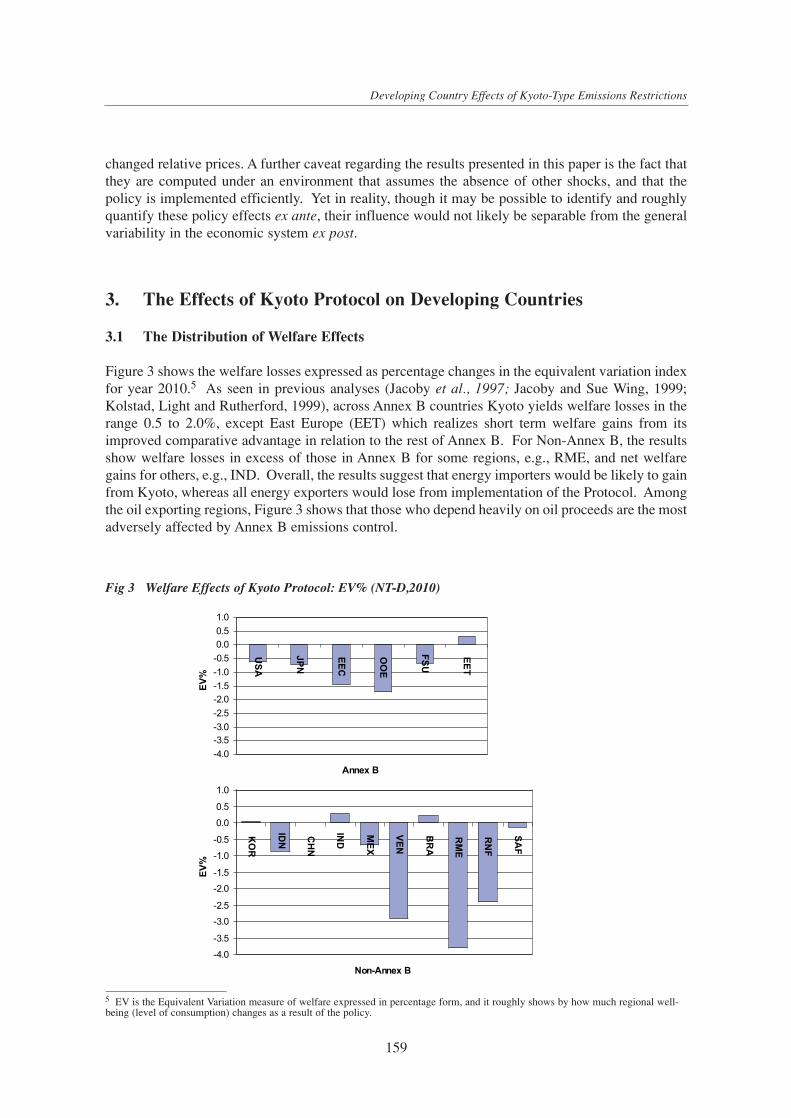
changed relative prices. A further caveat regarding the results presented in this paper is the fact thatthey are computed under an environment that assumes the absence of other shocks, and that thepolicy is implemented efficiently. Yet in reality, though it may be possible to identify and roughlyquantify these policy effects ex ante, their influence would not likely be separable from the generalvariability in the economic system ex post.
3. The Effects of Kyoto Protocol on Developing Countries
3.1 The Distribution of Welfare Effects
Figure 3 shows the welfare losses expressed as percentage changes in the equivalent variation indexfor year 2010.5 As seen in previous analyses (Jacoby et al., 1997; Jacoby and Sue Wing, 1999;Kolstad, Light and Rutherford, 1999), across Annex B countries Kyoto yields welfare losses in therange 0.5 to 2.0%, except East Europe (EET) which realizes short term welfare gains from itsimproved comparative advantage in relation to the rest of Annex B. For Non-Annex B, the resultsshow welfare losses in excess of those in Annex B for some regions, e.g., RME, and net welfaregains for others, e.g., IND. Overall, the results suggest that energy importers would be likely to gainfrom Kyoto, whereas all energy exporters would lose from implementation of the Protocol. Amongthe oil exporting regions, Figure 3 shows that those who depend heavily on oil proceeds are the mostadversely affected by Annex B emissions control.
159
Developing Country Effects of Kyoto-Type Emissions Restrictions
5 EV is the Equivalent Variation measure of welfare expressed in percentage form, and it roughly shows by how much regional well-being (level of consumption) changes as a result of the policy.
-4.0
-3.5
-3.0
-2.5
-2.0
-1.5
-1.0
-0.5
0.0
0.5
1.0
KOR
IDN
CHN
IND
MEX
VEN
BRA
RME
RNF
SAF
Non-Annex B
EV%
-4.0
-3.5
-3.0
-2.5
-2.0
-1.5
-1.0
-0.5
0.0
0.5
1.0
USA
JPN
EEC
OOE
FSU
EET
Annex B
EV%
Fig 3 Welfare Effects of Kyoto Protocol: EV% (NT-D,2010)
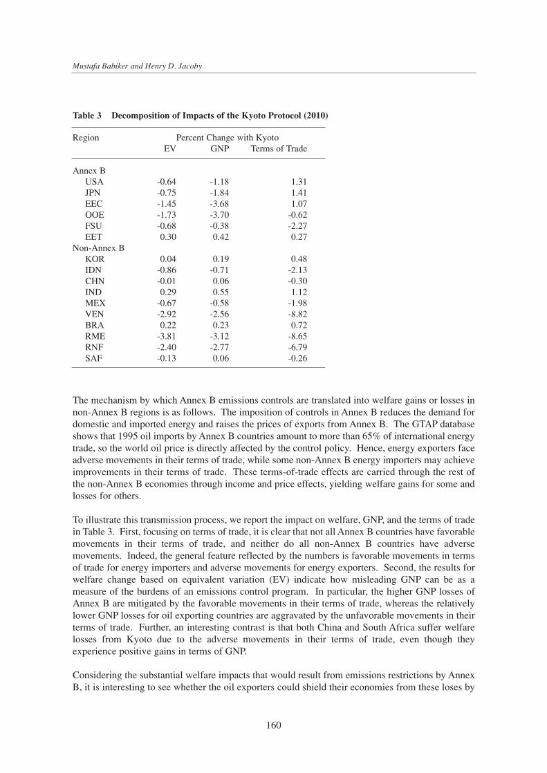
The mechanism by which Annex B emissions controls are translated into welfare gains or losses innon-Annex B regions is as follows. The imposition of controls in Annex B reduces the demand fordomestic and imported energy and raises the prices of exports from Annex B. The GTAP databaseshows that 1995 oil imports by Annex B countries amount to more than 65% of international energytrade, so the world oil price is directly affected by the control policy. Hence, energy exporters faceadverse movements in their terms of trade, while some non-Annex B energy importers may achieveimprovements in their terms of trade. These terms-of-trade effects are carried through the rest ofthe non-Annex B economies through income and price effects, yielding welfare gains for some andlosses for others.
To illustrate this transmission process, we report the impact on welfare, GNP, and the terms of tradein Table 3. First, focusing on terms of trade, it is clear that not all Annex B countries have favorablemovements in their terms of trade, and neither do all non-Annex B countries have adversemovements. Indeed, the general feature reflected by the numbers is favorable movements in termsof trade for energy importers and adverse movements for energy exporters. Second, the results forwelfare change based on equivalent variation (EV) indicate how misleading GNP can be as ameasure of the burdens of an emissions control program. In particular, the higher GNP losses ofAnnex B are mitigated by the favorable movements in their terms of trade, whereas the relativelylower GNP losses for oil exporting countries are aggravated by the unfavorable movements in theirterms of trade. Further, an interesting contrast is that both China and South Africa suffer welfarelosses from Kyoto due to the adverse movements in their terms of trade, even though theyexperience positive gains in terms of GNP.
Considering the substantial welfare impacts that would result from emissions restrictions by AnnexB, it is interesting to see whether the oil exporters could shield their economies from these loses by
160
Mustafa Babiker and Henry D. Jacoby
Table 3 Decomposition of Impacts of the Kyoto Protocol (2010)
Region Percent Change with KyotoEV GNP Terms of Trade
Annex BUSA -0.64 -1.18 1.31JPN -0.75 -1.84 1.41EEC -1.45 -3.68 1.07OOE -1.73 -3.70 -0.62FSU -0.68 -0.38 -2.27EET 0.30 0.42 0.27
Non-Annex BKOR 0.04 0.19 0.48IDN -0.86 -0.71 -2.13CHN -0.01 0.06 -0.30IND 0.29 0.55 1.12MEX -0.67 -0.58 -1.98VEN -2.92 -2.56 -8.82BRA 0.22 0.23 0.72RME -3.81 -3.12 -8.65RNF -2.40 -2.77 -6.79SAF -0.13 0.06 -0.26

controlling oil price, by restricting oil production. To explore this question we simulate a case inwhich OPEC countries restrict output in order to maintain the baseline oil price trajectory. Theresulting oil production profiles are shown on Figure 4, and the welfare consequences relative to theKyoto Protocol without such an action are shown in Figure 5. Figure 4 shows that OPEC regionswould have to cut their production by 40% to prevent the international price of oil from falling,given the reduced demand in Annex B in response to the carbon constraint, and the increased outputby non-OPEC oil exporters. The net welfare result, shown in Figure 5, reveals large welfare lossesfor OPEC members, additional welfare costs for Annex B and the oil importing non-Annex Bregions, and, of course, welfare gains for non-OPEC oil exporters. Relative to Kyoto with no OPECresponse, the welfare repercussions suggested by Figure 5 amount to an average 6-15% increase incost for the oil-importing Annex B, but a more than doubling of the welfare loss for the OPECregions6. With such significant potential welfare losses in OPEC, it seems the chances for such aresponse to Kyoto are small.
3.2 Carbon Leakage
Carbon leakage is the increase in carbon emissions in the non-abating regions resulting from therelative price and income effects generated by carbon restrictions in the abating regions. Leakageis usually stated as a percentage of the total cutback in emissions by countries under restriction. Inparticular, the abatement action in Annex B raises the production costs of energy intensive goodsand encourages the offshore production of these goods. Also, the fall in Annex B demand forimported oil puts downward pressure on the international price of oil and encourages its use in Non-Annex B regions. The combination of the shift in non-Annex B comparative advantage in energy-intensive production, together with the fall in energy prices, is likely to increase carbon emissions
161
Developing Country Effects of Kyoto-Type Emissions Restrictions
-50
-40
-30
-20
-10
0
10
20
IDN
MYS
FSU
MEX
VEN
COL
RME
RNF
RSS
Region
%
6 These results are sensitive to the details of the EPPA-GTAP model structure, including the assumed structure of the energy marketsand the sub-model of resource supply.
Figure 4 OPEC Cartel and Kyoto: Change in Oil Production Profiles from Reference (NT-D, 2010)

in non-Annex B above their baseline trajectories. This phenomenon is illustrated in Figure 6, whichshows the net exports of energy-intensive goods for the Annex B regions and for those Non-AnnexB regions that we highlight here. Exports from the OECD fall with the imposition of the Kyotorestrictions (with the USA becoming a net importer). The FSU and EET (whose Kyoto restrictionsdo not bind in 2010) increase exports, as do a number of Non-Annex B countries, while all theothers lower their net imports.
EPPA-GTAP shows a global leakage rate of 6% for 2010, which is in line with that reported forGREEN (OECD, 1992), the G-Cubed model (McKibbin et al., 1999), and with results from EPPA-GREEN (Jacoby et al., 1997). Nevertheless, compared to other studies (e.g., Babiker et al, 1997;Felder and Rutherford, 1993; Kolstad et al, 1999), this leakage rate is somewhat lower. One reasonwhy we have lower leakage rate compared to models other than GREEN is the way existingdistortions in the energy markets are treated. In particular, both GREEN and EPPA-GTAP phaseout energy subsidies and balance of payment deficits along the baseline whereas other models donot. Simulating the model under the existing subsidies, we found global leakage would increase to8% in 2010. The contributions of a selection of developing countries to the global leakage rate isshown in Figure 7. The two main features from the figure are that 30% of the leakage is contributed
162
Mustafa Babiker and Henry D. Jacoby
-12-11-10
-9-8-7-6
-5-4-3-2
-101
USA
JPN
EEC
OOE
FSU
EET
Annex B
EV% OPEC
N-OPEC
-12
-11
-10
-9
-8
-7
-6
-5
-4
-3
-2
-1
0
1
KOR
IDN
CHN
IND
MEX
VEN
BRA
RME
RNF
SAF
Non-Annex B
EV%
OPEC
N-OPEC
Figure 5 Welfare Effects of OPEC Price Control Relation to Kyoto Protocol with no OPEC Response(NT-D, 2010)

163
Developing Country Effects of Kyoto-Type Emissions Restrictions
-20
-10
0
10
20
30
40
50
60
USA JPN EEC OOE FSU EET
AnnexB
b1995$
Ref
Kyoto
-60
-50
-40
-30
-20
-10
0
10
20
KOR IDN CHN IND MEX VEN BRA RME RNF SAF
Non-AnnexB
b1995$
Ref
Kyoto
0
0.4
0.8
1.2
1.6
2
KOR IDN CHN IND MEX VEN BRA RME RNF SAF
Region
%
Figure 6 Net Exports of Energy-Intensive Products with Kyoto Protocol (NT-D, 2010)
Figure 7 Carbon Leakage Rates Under Kyoto Protocol (NT-D, 2010)
by China alone and that more than 60% of the leakage is contributed by five key countries: China,India, Brazil, South Korea, and Mexico. This would suggest that an effective policy to curtailleakage will have to focus on these countries.
4. Implications of Alternative Annex B Policy Designs
Most analyses of Kyoto-type emissions agreements assume that the policy is imposed as a uniformtax on fossil fuels, or by means of a cap-and-trade system that results in a common price of carbonemissions across sources. One can even think of such calculations as approximating the results of asystem of regulatory measures so calibrated as to yield a common marginal cost of carbon reductionacross all sources. But the circumstances, in reality, are more complicated than what suchcalculations imply, because the fiscal systems of many countries, particularly in Europe, have formany decades used fuel taxes as an important source of revenue. Others, like the United States, havea different fiscal tradition, and use these taxes far less.
The fact that the GTAP database identifies these fiscal distortions provides an opportunity to explorethe implications of different ways of imposing the Kyoto restrictions. Countries could harmonizefuel taxes on a common carbon basis, yielding a uniform carbon-equivalent tax across all fuels. Onthe other hand, and more likely, the existing fiscal measures might be left intact, with any carbontaxes or permit fees simply imposed in a supplemental manner. Though, in practice the result islikely to be some blend of the two, a simple comparison between the two polar cases providesinsight as to the implications of the choice for developing countries. In the welfare comparisons wedo not compensate for the possible difference in revenue within Annex B countries between the twocases, implicitly assuming that any loss or gain in revenue due to an abandonment of non-carbonfuel taxes is made up with a non-distorting lump-sum levy.7
The comparison is shown in Figure 8. Looking first at the Annex B countries, shown in the lowerpart of the figure, it can be seen that a switch to a harmonized carbon-based increase in fuel pricesis favorable to all regions. The gain is greatest in Europe because the distortions are greatest there.
Interestingly, a choice of harmonized as compared to distorted fuel surcharges is beneficial to Non-Annex B countries as well, as seen in the upper part of the figure. For the oil exporting regions thereason for this effect is straightforward to explain.8 Recall that the increase in world oil price, inrelation to the reference, is only 9% if harmonized taxes are applied, whereas the increase is 15% ifexisting distortions are maintained. Thus with a harmonized system, the deterioration in terms oftrade of the oil exporters is reduced, reducing their welfare loss.
164
Mustafa Babiker and Henry D. Jacoby
7 Our calculation is not exactly equivalent to the tax treatment in most analyses of the double-dividend issue because we do not imposethe condition that the revenue raised from the taxing system remains the same, i.e., it is not revenue neutral for the tax-collecting agent.However, imposition of a revenue-neutrality condition would not likely change the implications for Non-Annex B countries of theremoval of these distortions.
8 Given the complex general equilibrium process involved, the reason why other Non-Annex B regions are better off requires furtheranalysis. One possible explanation is the removal of existing distortions in Annex B increases their demand for oil (compared to thedistortion case) and reduces the export price of their energy intensive goods to Non-Annex B.

5. Effects of Emissions Trading
The details of international emissions trading, covered under Article 17 of the Kyoto Protocol(United Nations, 1997) are the subject of continuing debate within the Conference of Parties.Although the complexities of alternative implementation schemes may prevent attainment of thecost savings of an ideal trading regime (Hahn and Stavins, 1999), many studies have shown that thepotential for cost reductions is great (e.g., Montgomery et al., 1998; Jacoby et al., 1997; OECD,1992). The analysis conducted here shows the same result. The gains from emissions trading aresubstantial not only for those engaging in the trade, but often for others as well. We consider twosuch cases: (1) trading within Annex B alone, and (2) Annex B trading with participation by China,to illustrate the implications of extending the regime to include developing countries.
The results are shown in Figure 9. Consider first the Annex B countries, and the case where onlythey can trade emissions permits. Given our reference forecast, the FSU and the EET together have165 MtC of “hot air” in 2010. They benefit from selling it, and the four OECD regions benefit fromthe lowered cost of carbon control. In the United States, for example, the carbon price in 2010 dropsfrom $205 per ton under autarchy to $92 with Annex B trading. In welfare terms, the cost is loweredmost in Japan (by 58%), and in the rest of OECD regions as well (by 28% to 40%) compared to thecase of no emissions trading.
165
Developing Country Effects of Kyoto-Type Emissions Restrictions
-4.0
-3.5
-3.0
-2.5
-2.0
-1.5
-1.0
-0.5
0.0
0.5
1.0
KO
R
IDN
CH
N
IND
ME
X
VE
N
BR
A
RM
E
RN
F
SA
F
Non-annex B
%
NT-H
NT-D
-4.0
-3.5
-3.0
-2.5
-2.0
-1.5
-1.0
-0.5
0.0
0.5
1.0
US
A
JPN
EE
C
OO
E
FS
U
EE
T
Annex B
%
NT-H
NT-D
Figure 8 Kyoto and Welfare: The Implication of Pre-existing Distortions In Annex B’s Energy Markets(2010)
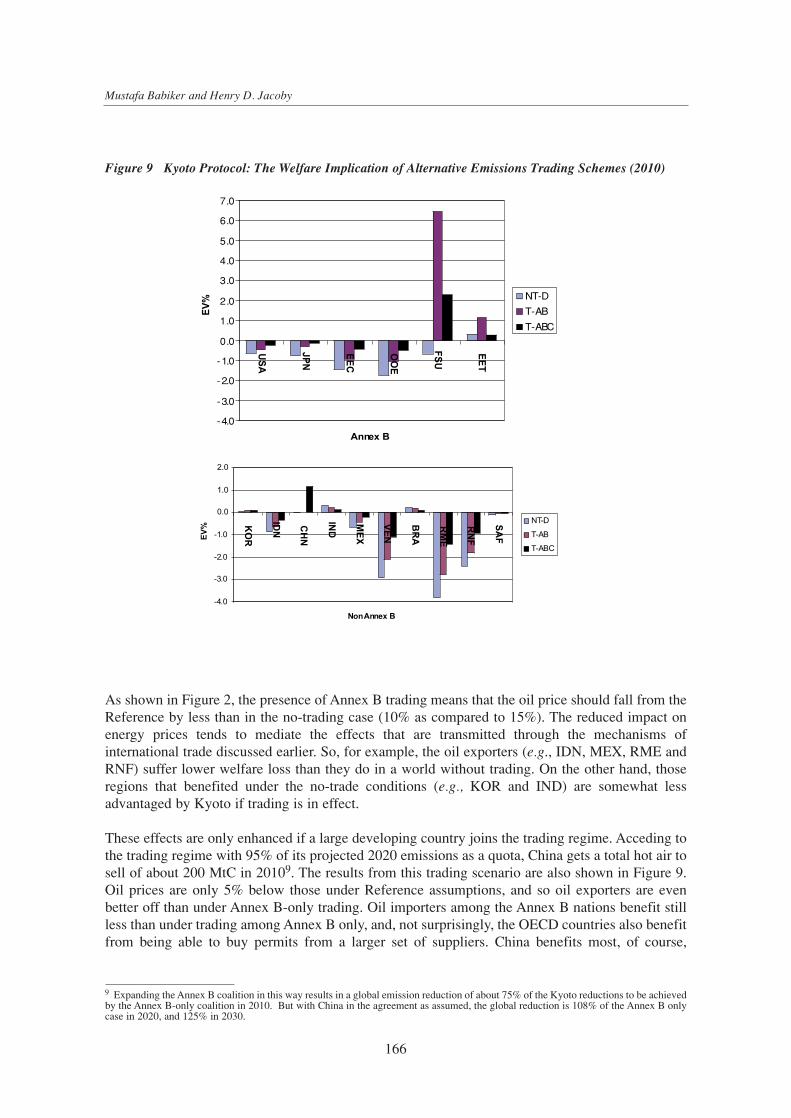
As shown in Figure 2, the presence of Annex B trading means that the oil price should fall from theReference by less than in the no-trading case (10% as compared to 15%). The reduced impact onenergy prices tends to mediate the effects that are transmitted through the mechanisms ofinternational trade discussed earlier. So, for example, the oil exporters (e.g., IDN, MEX, RME andRNF) suffer lower welfare loss than they do in a world without trading. On the other hand, thoseregions that benefited under the no-trade conditions (e.g., KOR and IND) are somewhat lessadvantaged by Kyoto if trading is in effect.
These effects are only enhanced if a large developing country joins the trading regime. Acceding tothe trading regime with 95% of its projected 2020 emissions as a quota, China gets a total hot air tosell of about 200 MtC in 20109. The results from this trading scenario are also shown in Figure 9.Oil prices are only 5% below those under Reference assumptions, and so oil exporters are evenbetter off than under Annex B-only trading. Oil importers among the Annex B nations benefit stillless than under trading among Annex B only, and, not surprisingly, the OECD countries also benefitfrom being able to buy permits from a larger set of suppliers. China benefits most, of course,
166
Mustafa Babiker and Henry D. Jacoby
-4.0
-3.0
-2.0
-1.0
0.0
1.0
2.0
3.0
4.0
5.0
6.0
7.0
USA
JPN
EEC
OOE
FSU
EET
Annex B
EV% NT-D
T-AB
T-ABC
-4.0
-3.0
-2.0
-1.0
0.0
1.0
2.0
KOR
IDN
CHN
IND
MEX
VEN
BRA
RME
RNF
SAF
NonAnnex B
EV%
NT-D
T-AB
T-ABC
9 Expanding the Annex B coalition in this way results in a global emission reduction of about 75% of the Kyoto reductions to be achievedby the Annex B-only coalition in 2010. But with China in the agreement as assumed, the global reduction is 108% of the Annex B onlycase in 2020, and 125% in 2030.
Figure 9 Kyoto Protocol: The Welfare Implication of Alternative Emissions Trading Schemes (2010)

because of its hot air and because of having low-cost opportunities for reducing its carbon emissionsbelow the baseline level. The big loser is the FSU. It is better of than with no trading at all, but itwould much prefer not to have to sell its hot air in competition with China.10
6. Summary and Conclusions
It is no surprise that emissions control actions by the large developing countries, who dominateworld trade flows, can have ripple effects on the global economy, influencing countries who havenot volunteered to share any burdens of the regime of emissions control. The magnitudes of theseimpacts are highly uncertain, but the analysis above does give an idea of what these impacts mightbe, as well as how they are transmitted through the international trade system. Clearly, the greatestloss is imposed on energy exporters, and the more dependent a country is on these exports thegreater the percentage effect on its economic welfare. So a country like Mexico, with a large anddiversified economy is much less influenced than the nations of the Persian Gulf (RME), for whomoil revenues constitute a large faction of GNP. Moreover, according to our analysis there is not muchthat the exporters can do about it, say through coordinated efforts by OPEC. The elasticities ofdemand by importing countries, and of supply by the non-OPEC exporters, combine to produce amarket condition where efforts to resist the fall in oil price resulting from Kyoto restrictions lead tostill lower overall OPEC revenue. Attempts to do the same by a smaller group within OPEC wouldlead to even worse results for those taking action to support the price. Recall, of course, that theseresults are for 2010, and in the longer term the relevant elasticities could change, influencing thisresult.
Moreover, details of the process of implementation of Kyoto-type agreements matter to the Non-Annex B countries. The distribution of burdens differs depending on the treatment of existing fuelstaxes in the enacting of carbon policies; and the presence or absence of emissions trading is evenmore significant. One troublesome result of these studies, however, is the observation that Non-Annex B countries do not necessarily have a common interest in these details. Within the bounds ofuncertainty in this issue the lists of winners and losers among Non-Annex B could shift somewhat,but the fact would remain that interests conflict within the group. In general, those importing energywill benefit from more stringent the policies, and the energy exporters will lose. Moreover,emissions trading and tax harmonization will look different depending on a nation’s position on thisscale. The intensity of the response will be approximately in proportion to the weight of the energysector in the national economy.
167
Developing Country Effects of Kyoto-Type Emissions Restrictions
10 For further exploration of trading scenarios, see Ellerman, Jacoby and Decaux (1998).
References
Babiker, M. H., J. Reilly, and I. Sue Wing (1999). TheEmissions Prediction and Policy Analysis (EPPA)Model: Update, Sensitivity, and Comparison of Results,in progress.
Babiker, M. H., K. E. Maskus and T. F. Rutherford (1997).Carbon Tax and the Global Trading System, WorkingPaper, (97-7). University of Colorado, Boulder.
Burniaux, J., G. Nicoletti and J. Oliveira-Martin (1992).GREEN: A Global Model for Quantifying the Cost ofPolicies to Curb CO2 Emissions, OECD EconomicStudies No. 19, Winter: 49-92.
DOE/EIA (1998). International Energy Outlook.Ellerman, A. D., H.D. Jacoby, and A. Decaux (1998). The
Effects on Developing Countries of the Kyoto Protocoland CO2 Emissions Trading, MIT Joint Program on theScience and Policy of Global Change, Report No. 41,Cambridge, MA.
Felder, Stefan and T. Rutherford (1993). Unilateral CO2Reductions and Carbon Leakage: the Effect ofInternational Trade in Oil and Basic Materials, Journalof Environmental Economics and Management, 25, 162-176.
Hahn, R. W. and R. N. Stavins (1999). What Has KyotoWrought? The Real Architecture of InternationalTradable Permit Markets, Working Paper, John F.Kennedy School of Government, Harvard University.
Hertel, T. W. (1997). Global Trade Analysis: Modeling andApplications, Cambridge: Cambridge University Press.
Jacoby, H. D., R. Eckaus, D. Ellerman, R. Prinn, D. Reiner,and Z. Yang (1997). CO2 Emissions Limits: EconomicAdjustments and the Distribution of Burdens, TheEnergy Journal, 18(3), 31-58.
Jacoby, H.D., and I. Sue Wing (1999). Adjustment Time,Capital Malleability, and Policy Costs, The EnergyJournal (Forthcoming – Kyoto Special Issue).
Jacoby, H. D., R. Schmalensee, and I. Sue Wing (1999).Toward a Useful Architecture for Climate Negotiations,MIT Joint Program on the Science and Policy of GlobalChange, in press.
Kolstad, C., M. Light, and T. Rutherford (1999). CoalMarkets and the Kyoto Protocol, Working paper,University of Colorado-Boulder.
McKibbin, W., M. Ross, R. Shackleton, and P. Wilcoxen(1999). Emissions Trading, Capital Flows and the KyotoProtocol, The Energy Journal (Forthcoming – KyotoSpecial Issue).
Montgomery, D., P. Bernstein, and T. Rutherford (1998).Carbon Abatement, Permit Trading and InternationalTrade, Working Paper. Charles River Associates andUniversity of Colorado, Boulder.
OECD (1992). The Economic Costs of Reducing CO2Emissions, Paris, France: OECD.
Portney, P.R. (1999). The Joy of Flexibility: U.S. ClimatePolicy in the Next Decade. Keynote Address to NationalEnergy Modeling System/Annual Outlook Conference,U.S. Energy Information Administration, March 12.
Reilly, J. M. et al. (1999). Multi-gas Assessment of theKyoto Protocol, MIT Joint Program on the Science andPolicy of Global Change, Report No. 45, MIT,Cambridge, MA. (Forthcoming in nature)
Untied Nations (1997). Kyoto Protocol to the UnitedNations Framework Convention on Climate Change,Conference of the Parties on Its Third Session,FCCC/CP/1997/L.7/Add.1, 10 December.
Webster, M. D., 1997. Exploring the Uncertainty in FutureCarbon Emissions, Report No. 30, Joint Program on theScience and Policy of Global Change, MIT, Cambridge,MA.
Webster, M. D., and Sokolov, A., 1998. Quantifying theUncertainty in Climate Predictions, Report No. 37, JointProgram on the Science and Policy of Global Change,MIT, Cambridge, MA.
Yang, Z., R. S. Eckaus, A. D. Ellerman and H. D. Jacoby(1996). The MIT Emission Projection and PolicyAnalysis (EPPA) model, MIT Joint Program on theScience and Policy of Global Change, Report No. 5,MIT, Cambridge, MA.
168
Mustafa Babiker and Henry D. Jacoby

The IPCC-SRES Stabilisation Scenarios
Johannes Bollen1, Ton Manders2, Hans Timmer2
We analyse both the macro economic impacts and the effects on energy markets of imposing globalconstraints of CO2 emissions, given that on the medium term the Annex-1 region (OECD regionsand Economies in Transition) will undertake the abatement effort and comply with the Kyotoprotocol, and for the longer term some all NA-1 countries gradually, based on a welfare trigger, willjoin the A-1 group of countries. The aim of the global CO2 constraint is stabilize concentrations at550 ppmv. Starting point is the calibration of the new A1 scenario, which is used as the ‘Business-As-Usual’ scenario1 and developed with the Applied General Equilibrium model WorldScan. Weshow how a specific burden sharing rule yields different regional target profiles, depending onwhether the global policy calls for an early action or a delayed response. It is shown that by applyinga system of tradable permits to achieve a global constraint, new partners can be attracted to join theabatement coalition. But it is also shown that some countries within the abatement coalition mightbe against entry of any new partners. Also we will illustrate that the evolution of permit markets willbe less stable in a situation of early action than with a delayed response.
1 Introduction
The Kyoto protocol states that countries belonging to Annex-1 (A-1) will take the lead in limitinggreenhouse gas emissions. Other members of the Framework on the Convention of Climate Change(FCCC), the Non-Annex-1 (NA-1) countries, do not have to sign up to targets. The negotiationsunder the FCCC have proven to be very difficult. Why so? The answer can be found in the differentinterests of the countries around the negotiation table, originating from differing contributions to thecumulation of greenhouse gases in the atmosphere, and diverging economic interests in doing so.
The Parties to the FCCC have introduced three new instruments under the Protocol, allowing Parties(or entities) with emission limits to achieve emission reductions outside their national borders.There are three mechanisms for transferring the emissions internationally under the protocol: JointImplementation (JI), International Emission Trading (IET) and Clean Development Mechanism(CDM) .
• Joint Implementation (JI) concerns project-level credits, labeled Emission Reduction Units(ERU’s) as defined in Article 6, transferable among Annex I Parties.
169
The IPCC-SRES Stabilisation Scenarios
1 National Institute of Public health and the Environment (RIVM), P.O. Box 2, 3720 BA Bilthoven, the Netherlands
2 CPB Netherlands Bureau for Economic Policy Analysis (CPB), van Stolkweg 14, P.O. Box 80510, The Hague, the Netherlands
3 Please note that the we participated in collaboration with the RIVM IMAGE team in the development of the scenarios for the IPCCSpecial Report on Emissions Scenarios (SRES). Calculations in this report are based on input from the modeling teams participating inSRES and explore how SRES-type scenarios could be used for mitigation analysis. They are necessarily preliminary, since the SRESscenarios have not been approved by IPCC and are therefore subject to changes.

• International Emission Trading (IET), as defined in Article 17 of the Protocol, concerns transferof the Assigned Amounts (AA’s) among Annex-1 Parties, which are applicable in the first budgetperiod, running from 2008 till 2012. The AA’s are corrected for Certified Emission Reductions(CER) obtained from CDM projects.
• Clean Development Mechanism (CDM) concerns CER’s, as defined in Article 12, transferablefrom non Annex I Parties to Annex I Parties
The first two instruments can reduce the total costs of emission reductions within the Annex Iregion, because they create the option to realize reductions in those countries where marginalabatement costs are lowest. From an Annex I perspective, the third instrument can be seen as anextension of this flexibility to the global level. Since costs of emission reduction are relatively lowoutside the Annex I area, this global flexibility should further reduce costs for Annex I Parties.
This report focuses on the application of the first flexible instrument only. This instrument isassumed to be applied both within the time frame of the Kyoto protocol, but also beyond 2010. Thisreport is also an attempt to address the some of the issues related to the economics of when-flexibility (see Nature, 1996). We will use prescribed global pathways of emissions (aiming atstabilization of atmospheric concentrations by the year 2100) as the starting point of our analysis.
This report does not address legal issues of enlargement of the abatement coalition nor the topic ofimplementation of a tradable permit market. This report attempts to highlight some of the macro-economic impacts of implementing targets as described in the Kyoto protocol, based on simulationswith WorldScan.
The organization of the report is as follows. First a short description of the model will be presented.Second, a short description of the A1 baseline scenario will be given. Also the feasible policystrategy will be described within the context of the A1 baseline scenario. This strategy aims for asignificant reduction of CO2 emissions due to fuel combustion, and hence a lower CO2concentration in the atmosphere. Third, since the feasible policy strategies leads to a gradualextension of the current abatement group of countries, some theoretical notions will be presented onthe impacts of enlarging the abatement coalition. The report will finalize with an overview of themain findings of the results and conclusions of the model simulations.
2 Overview of the model
WorldScan has been developed to construct scenarios. To avoid extrapolation of current trends ormere reproduction of the current situation, WorldScan relies on the neoclassical theories of growthand international trade. Changes in economic growth and international specialization patternsevolve from changes in (relative) endowments. The emphasis on the long run also manifests itselfin the broad definition of sectors. The WorldScan Core model distinguishes 11 sectors. This is arelatively small number compared to other AGE models. Over a long period of two decades or morethe character of products and branches of industry change drastically. Current statistical definitionsof products and branches of industry are likely to become irrelevant at the end of scenario period.For this reason, WorldScan uses broad aggregates.
170
Bollen J.C., Manders T. and Timmer H.

The standard neoclassical theory of growth distinguishes three factors to explain changes inproduction: the accumulation of physical capital, labor, and a fixed technology trend. WorldScanaugments the simple growth model in three ways. First, WorldScan allows overall technology todiffer across countries. It also takes up the related idea that developing countries can catch upquickly by adopting foreign state-of-the-art technologies. Second, the model distinguishes two typesof labor: high-skilled and low-skilled labor. Sectors differ according to the intensity with which theyuse high-skilled and low-skilled labor. Countries can raise per capita growth by schooling andtraining the labor force. Third, in developing countries part of the labor force works in low-productivity sectors. In these sectors workers do not have access to capital and technology.Reallocation of labor from the low-productivity sectors to the high-productivity sectors enablescountries to raise per capita growth as well. In principle, all these three factors affect theperformance of a region only temporarily. Catching-up, training of low-skilled workers andreallocating labor to the high-productivity sector do not raise the growth rate indefinitely.Nevertheless, they are important. Adjustments in the economies of developing regions take a greatdeal of time and will surely show up in the growth rates of these regions in the period underconsideration.
171
The IPCC-SRES Stabilisation Scenarios
The WorldScan Core model Compared to the standard neoclassical theories of economic growth and international trade,worldScan is extended to add realism to scenarios. In doing so, we aim at bridging the gapbetween academic and policy discussions. The extensions include:
- an Armington trade specification, explaining two-way trade and allowing market power todetermine trade patterns in the medium run, while allowing Heckscher-Ohlin mechanisms inthe long run;
- imperfect financial capital mobility;- consumption patterns depending upon per capita income, and developing towards a
universal pattern;- a Lewis-type low-productivity sector in developing regions, from which the high-
productivity sector can draw labour, enabling high growth for a long period.
The model distinguishes the following regions, sectors and productive:
Regions Sectors Productive factors
United States U Agriculture L Primary inputsWestern Europe W Services W Low-skilled labourJapan J Trade and Transport D High-skilled labourRest of the OECD P Electricity J CapitalEastern Europe E Intermediate goods I Fixed factorFormer Soviet Union F Consumer goods CMiddle East and North Africa M Capital goods M Intermediate inputsSub-Saharan Africa S Other Raw Materials R from all sectorsLatin America LChina CSouth-East Asia NSouth Asia & Rest O
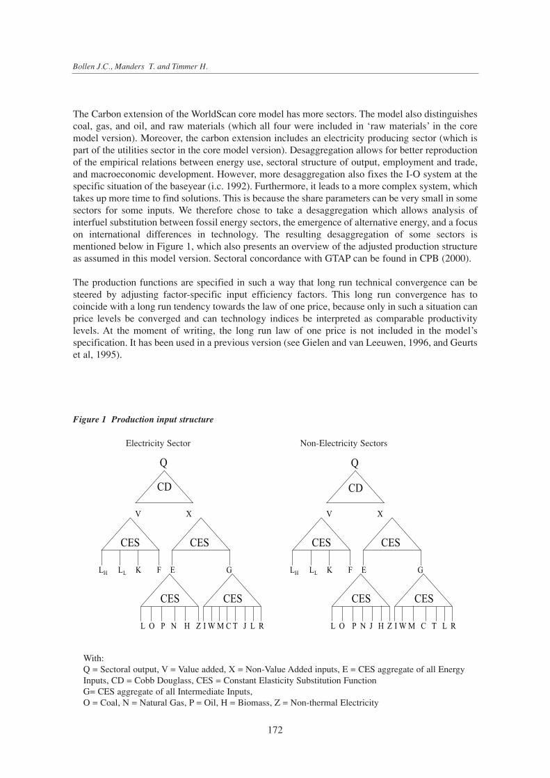
The Carbon extension of the WorldScan core model has more sectors. The model also distinguishescoal, gas, and oil, and raw materials (which all four were included in ‘raw materials’ in the coremodel version). Moreover, the carbon extension includes an electricity producing sector (which ispart of the utilities sector in the core model version). Desaggregation allows for better reproductionof the empirical relations between energy use, sectoral structure of output, employment and trade,and macroeconomic development. However, more desaggregation also fixes the I-O system at thespecific situation of the baseyear (i.c. 1992). Furthermore, it leads to a more complex system, whichtakes up more time to find solutions. This is because the share parameters can be very small in somesectors for some inputs. We therefore chose to take a desaggregation which allows analysis ofinterfuel substitution between fossil energy sectors, the emergence of alternative energy, and a focuson international differences in technology. The resulting desaggregation of some sectors ismentioned below in Figure 1, which also presents an overview of the adjusted production structureas assumed in this model version. Sectoral concordance with GTAP can be found in CPB (2000).
The production functions are specified in such a way that long run technical convergence can besteered by adjusting factor-specific input efficiency factors. This long run convergence has tocoincide with a long run tendency towards the law of one price, because only in such a situation canprice levels be converged and can technology indices be interpreted as comparable productivitylevels. At the moment of writing, the long run law of one price is not included in the model’sspecification. It has been used in a previous version (see Gielen and van Leeuwen, 1996, and Geurtset al, 1995).
172
Bollen J.C., Manders T. and Timmer H.
CES CES
LH LL K F
Q
CD
V X
I WM C T J L R
CES
E G
L O P N H Z
CES
CES CES
LH LL K F
Q
CD
V X
I WM C T L R
CES
E G
L O P N J H Z
CES
With:Q = Sectoral output, V = Value added, X = Non-Value Added inputs, E = CES aggregate of all EnergyInputs, CD = Cobb Douglass, CES = Constant Elasticity Substitution FunctionG= CES aggregate of all Intermediate Inputs, O = Coal, N = Natural Gas, P = Oil, H = Biomass, Z = Non-thermal Electricity
Figure 1 Production input structure
Electricity Sector Non-Electricity Sectors
The model is benchmarked to the GTAP4E data set, see Mc Dougall et all. (1998). The calibrationyear is 1995. From this data base we derive not only demand, production and trade patterns, but alsolabour and capital intensity of the various sectors. The sectoral classification according to skillintensity is broadly correct, but the precise differences could very well change, when better databecome available.
Population trajectories follow those of the A1 Narrative. The ILO (1996) provides participation ratesfor the base year, and for the years up to 2100 they follow the trend of the share of the 15-60 yearcohorts. The data for the supply of low-skilled and high-skilled workers at a regional level havebeen taken from Ahuja and Filmer (1995). Workers are labelled high-skilled when they havecompleted secondary education or a higher level. Ahuja and Filmer provide projections for manydeveloping countries. We lack projections for the OECD, Eastern Europe and the Former SovietUnion. Therefore we use the Barro and Lee (1996) data on education. We derive a trend betweenOECD and non-OECD regions between 1960 and 1990 and extrapolate this trend until 2100. Thedata on the size of the informal sector are obtained from the WorldBank (1995) and the ILO (1998).
Energy data in GTAP4E is an improvement over previous data like in GTAP4. This improvementis due to the incorporation of data on energy volumes prices provided by IEA (1997). Implicit pricesresult from the confrontation of the value of output and trade per region in GTAP4 with volume dataof output and trade. The difference between domestic prices and internationally traded prices ismatched by energy subsidies.
Data on the input of biofuels and renewables is drawn from IMAGE. From IMAGE we derive thevolume data on the use of biofuels and renewables (as a percentage of fossil fuels). We assumeprices to equal prices of agriculture and services, respectively.
3 Feasible Policy Strategies in the A1 Narrative
This scenario is dominated by moderate high economic growth with the emphasis on globaltechnological convergence, and strongly intensified trade linkages. The population growth isrelatively low, with a decline of the global population after 2050. The energy intensive sectorsdevelop technologies which lead to relatively low energy demand, with a sharp decarbonizationafter 2050. The emphasis of the people in this scenario is to maximize income, rather than to pursueany environmental objectives.
In order to analyze the potential impacts of additional climate policies within this narrative, two setsof different global emission profiles are used. Both these profiles only refer to the fossil energyrelated emissions, and are assumed to stabilize CO2 emissions at 550ppmv4. The first is one ofimmediate action and the second is a delayed version of the first. This approximately means that thecumulative emissions over the 1995-2100 period are the same. We start with the Kyoto protocol,followed by the entrance of some non Annex I regions. In the A1 scenario climate agreements areassumed to be feasible, but only as an extension of the Kyoto protocol. The A1 narrative tells us thatalthough regions pursue market-oriented policies, it does not exclude incentives for governments toagree on a significant carbon abatement effort. The wealthy nations take the responsibility of
173
The IPCC-SRES Stabilisation Scenarios
4 Unfortunately, the global emission profiles presented in this paper lie below 550 ppmv, but will be adjusted in a next version of thisexercise to make the calculations comparable with other models.

matching the global reduction profile and thus implement an international environmentalagreement. The creation of a international Annex I permit market with gradual extensions isconsistent with the narrative characteristics of the A1 baseline scenario. The establishment of aninternational permit market is believed to be the minimal required policy instrument to combatclimate change. Governments under the FCCC have the power to agree on protocols which willextend the Kyoto protocol and introduce new members to the Annex I group of countries by creatingadvantageous circumstances for these new members. The danger of assigning permits to regions thatlead to hot-air trade is present, but this is still regarded as a long term restriction of the emissions ofthese new members countries. But the speed at which governments are actually capable to attractnew members to the agreement differs. Welfare triggers are used to force entrance of new membersto the Annex I group of countries. The welfare trigger is set at 10000 US$ p.c. for both the delayedresponse as well as the early action scenario.
The regional Assigned Amount (AA) share distribution of the Kyoto protocol remains applicable forthe current Annex-1 group, up to the moment of entrance of new partners. After the entrance of anew partner, the residual for the old A-I group is calculated as the remainder of the global emissionprofile and the AA of the new partner. The AA amount of the new partner is defined to be constantfor a fixed period5. After this “grace period” the regional AA share distribution is upgraded, basedon the prevailing share distribution. The global constraint is always achieved, since the abatementgroup accounts for any carbon leakages to non-abating countries.
4 Permit Market Dynamics
Suppose that a country is acting on a permit market, e.g. in this case the former Soviet Union. Anillustration is given below in Figure 2, which shows some familiar marginal CO2 abatement costcurve: with on the y-axis the marginal costs of abatement and on the x-axis the level of abatement.Let us assume an agreed abatement level for the Former Soviet Union, being equal to t, at a givenequilibrium trade price level (FT). Total costs of abatement equals the surface labeled I. But sincethe equilibrium price level equals FT, the actual emission reduction exceeds the target level. Theactual reduction will equal tt. This implies that the total costs for the FSU equals the surface I minusII. This implies that the total costs are negative, and hence if a permit market is established the FSUwill surely gain from acting on this Annex I permit market, given the rules laid out in the protocol.
But, suppose now that other countries such as China enter the abatement coalition. There are severalreasons for joining the abatement group. First, A-1 countries could force them to do so, because itis cheaper to them to have more countries supply abatement technologies on the permit market. Inthis way the increasing burden of abatement is shared, but also it might lead to a tighter restrictionon the total allowed emission level. Secondly, as time evolves, NA-1 countries must increasinglyfeel the responsibility to reduce CO2 emissions, because in the end they also will become asignificant contributor to the built-up of greenhouse gas concentrations in the atmosphere. Finally,the regional external effects from global warming might actually persuade countries to join theAnnex I group of countries.
174
Bollen J.C., Manders T. and Timmer H.
3 The Kyoto protocol states for the current A-1 group of countries that by the end of the first commitment period emissions will equalthe AA’s. These AA’s are defined in terms of 1990 emission levels. An exception will be made for non-feasible reduction pathways oncethe necessary global emission reduction rate is too high).

How does this relate to Figure 2? Let us assume that there will be an additional player in theabatement group, and suppose that the required reduction effort in absolute terms for the newabatement group is the same as for the old one. Let us focus only on the former Soviet Union. Firstthere will be a reduction of the permit price, simply because the number of abatement technologiesfor the new abatement group is lager than for the old group. This means that the reduction effort ofthe FSU reduces to tt, at price equal to CFT. Hence the EEFSU costs of reduction reduces, but atthe same time the gains from trade reduces even stronger, and therefor the advantageous position ofthe former Soviet Union within the Annex I group in the Annex I trading case might not be sustainedfor the long run.
In general, expanding the abatement coalition, and setting less stringent restrictions on CO2emissions on countries in the “old” abatement coalition, may reduce the net costs of abatement ofcountries which are net-importers of permits and lower the benefits to net-exporters of permits.These benefits may even turn negative, at the expense of benefits or lower net costs to countieswhich join the abatement coalition. Hence, the reason to create a carbon coalition - and achieve areduction of potential welfare losses from abatement or increase the willingness to pursue anyabatement - and even bribe countries outside the coalition to join and experience income gains frompermit trade, at the same time reduces the incentive for the winners in the “old” coalition to remainwithin the coalition and agree with new entries. This will be illustrated with simulations with theWorldScan (WS) model.
However, we ignored in this example important macro-economic feedbacks that might significantlyaffect welfare of all countries, either within or outside the abatement coalition. Within the coalition,costs of abatement lead to welfare losses, although for some countries permit trade might have apositive effect on welfare. Generally, countries and regions not only are linked to each other viapermit trade, but also by trade of goods on other international markets (energy goods, and high and
175
The IPCC-SRES Stabilisation Scenarios
$/tC
FT
CFT
t tt
I
II
FSU
t
Figure 2 Costs of abatement for EEFSU when another country enters the abatement group
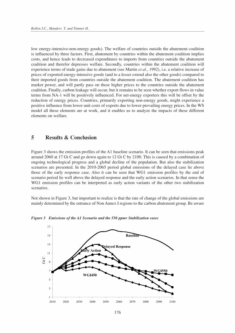
low energy-intensive-non-energy goods). The welfare of countries outside the abatement coalitionis influenced by three factors. First, abatement by countries within the abatement coalition impliescosts, and hence leads to decreased expenditures to imports from countries outside the abatementcoalition and therefor depresses welfare. Secondly, countries within the abatement coalition willexperience terms of trade gains due to abatement (see Martin et.al., 1992), i.e. a relative increase ofprices of exported energy-intensive goods (and to a lesser extend also the other goods) compared totheir imported goods from countries outside the abatement coalition. The abatement coalition hasmarket power, and will partly pass on these higher prices to the countries outside the abatementcoalition. Finally, carbon leakage will occur, but it remains to be seen whether export flows in valueterms from NA-1 will be positively influenced. For net-energy exporters this will be offset by thereduction of energy prices. Countries, primarily exporting non-energy goods, might experience apositive influence from lower unit costs of exports due to lower prevailing energy prices. In the WSmodel all these elements are at work, and it enables us to analyze the impacts of these differentelements on welfare.
5 Results & Conclusion
Figure 3 shows the emission profiles of the A1 baseline scenario. It can be seen that emissions peakaround 2060 at 17 Gt C and go down again to 12 Gt C by 2100. This is caused by a combination ofongoing technological progress and a global decline of the population. But also the stabilizationscenarios are presented. In the 2010-2065 period global emissions of the delayed case lie abovethose of the early response case. Also it can be seen that WG1 emission profiles by the end ofscenario period lie well above the delayed response and the early action scenarios. In that sense theWG1 emission profiles can be interpreted as early action variants of the other two stabilizationscenarios.
Not shown in Figure 3, but important to realize is that the rate of change of the global emissions aremainly determined by the entrance of Non Annex I regions to the carbon abatement group. Be aware
176
Bollen J.C., Manders T. and Timmer H.
1
3
5
7
9
11
13
15
17
2010 2020 2030 2040 2050 2060 2070 2080 2090 2100
GtC
Baseline
Delayed ResponseEarly Action
WGI550
WGI450
Figure 3 Emissions of the A1 Scenario and the 550 ppmv Stabilization cases

that the endogenously calculated carbon leakage from the abatement group to the non abatementgroup translates to sharper emission reductions of Annex I region. In the delayed case the Annex Igroup is allowed to increase its emissions, but mainly due to increased carbon imports by Annex Iregions from Latin America and the Dynamic Asian Economies entering the carbon abatementgroup in 2020 respectively 2025. Delayed action leads to much higher Annex I emissions by 2040(40% compared to early action), equalize by 2070, and are much lower by 2100 (35%) for all 550ppmv stabilization scenarios.
It should be pointed out here that the global cumulative emissions are equal for both stabilizationscenarios. As time evolves and more non Annex I countries join the carbon abatement, theiremissions start to stabilize and decline even after 2045. Carbon leakage rates are not presented here,but increase in the beginning of the scenario period, stabilize as well, and start to decrease as morecountries join the carbon abatement group. By 2100 Annex 1 emissions and Non Annex I emissionsare more or less of the same order.
But how does this relate to the actual assigned amounts? In Figure 4 the Permits p.c. are presentedfor both the OECD and the aggregate of Eastern Europe and the former Soviet Union (EEFSU).First focus on the period up to 2060. Here the differences are much more pronounced in terms ofthe two stabilization scenarios. In 2020, the OECD and EEFSU permits in the delayed case arealmost 100% higher than in the early action scenario, but they converge to it by 2055 and remainbelow afterwards. This implies that the burden of carbon abatement on Annex I economies is verydifferent in the delayed response scenario from the early action case, at least in the medium term. Itmay be expected that a world aiming for a stabilization of greenhouse gases in the atmosphere willshow the tendency of the initial abaters to start moderately with abatement and favor the delayedresponse scenario. After 2060 the regional permits p.c. are more or less the same for all Annex-1countries.
If we, however, take a closer look at the regional p.c. permits of the OECD in the long run (up to2100), it can be seen from Figure 5 that convergence of the p.c. permits of the OECD versus the
177
The IPCC-SRES Stabilisation Scenarios
0
0.5
1
1.5
2
2.5
3
3.5
2000 2010 2020 2030 2040 2050
TgC
OECD
EEFSU
Figure 4 Permits pc of the Stabilization Scenarios of the OECD and EEFSU regions for 2000-2050

Rest of the World (Africa, Middle East, and Latin America) occurs by 2085. In the delayed response scenario, all regions will experience a lower permit level than in the “early action” stabilizationscenario.
Below, Figure 6 presents the trade permit price level for the two scenarios for the 2000 – 2080period. After 2080, the difference between the price level of the two scenarios diverge so strongly,that the differences at the start of the next century do not show up anymore.
178
Bollen J.C., Manders T. and Timmer H.
1995
US$
/tC
Early Action
Delayed Response
2000 2010 2020 2030 2040 2050 2060 2070 2080
500
450
400
350
300
250
200
150
100
50
0
LAM
DYN
MEA
CHI AFR
IND
0
0.5
1
1.5
2
2.5
3
3.5
4
4.5
2000 2005 2010 2015 2020 2025 2030 2035 2040 2045 2050 2055 2060 2065 2070 2075 2080 2085 2090 2095 2100
OE RE
OD RD
OB RB
Figure 5 Permits pc of the Stabilization Scenarios of the OECD ROW regions for 2000-2100
Figure 6 Permit prices of the Stabilization scenarios for the 2000-2080 period
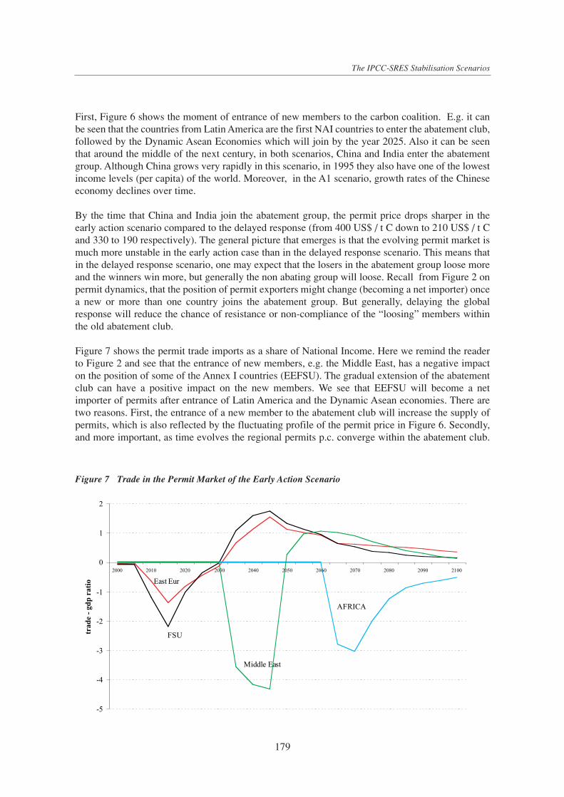
First, Figure 6 shows the moment of entrance of new members to the carbon coalition. E.g. it canbe seen that the countries from Latin America are the first NAI countries to enter the abatement club,followed by the Dynamic Asean Economies which will join by the year 2025. Also it can be seenthat around the middle of the next century, in both scenarios, China and India enter the abatementgroup. Although China grows very rapidly in this scenario, in 1995 they also have one of the lowestincome levels (per capita) of the world. Moreover, in the A1 scenario, growth rates of the Chineseeconomy declines over time.
By the time that China and India join the abatement group, the permit price drops sharper in theearly action scenario compared to the delayed response (from 400 US$ / t C down to 210 US$ / t Cand 330 to 190 respectively). The general picture that emerges is that the evolving permit market ismuch more unstable in the early action case than in the delayed response scenario. This means thatin the delayed response scenario, one may expect that the losers in the abatement group loose moreand the winners win more, but generally the non abating group will loose. Recall from Figure 2 onpermit dynamics, that the position of permit exporters might change (becoming a net importer) oncea new or more than one country joins the abatement group. But generally, delaying the globalresponse will reduce the chance of resistance or non-compliance of the “loosing” members withinthe old abatement club.
Figure 7 shows the permit trade imports as a share of National Income. Here we remind the readerto Figure 2 and see that the entrance of new members, e.g. the Middle East, has a negative impacton the position of some of the Annex I countries (EEFSU). The gradual extension of the abatementclub can have a positive impact on the new members. We see that EEFSU will become a netimporter of permits after entrance of Latin America and the Dynamic Asean economies. There aretwo reasons. First, the entrance of a new member to the abatement club will increase the supply ofpermits, which is also reflected by the fluctuating profile of the permit price in Figure 6. Secondly,and more important, as time evolves the regional permits p.c. converge within the abatement club.
179
The IPCC-SRES Stabilisation Scenarios
-5
-4
-3
-2
-1
0
1
2
2000 2010 2020 2030 2040 2050 2060 2070 2080 2090 2100
trade-gdpratio
FSU
East Eur
AFRICA
Middle East
Figure 7 Trade in the Permit Market of the Early Action Scenario

Therefore, EEFSU now experiencing a relatively low p.c. emission level, is faced as the OECDeconomies with new NAI members which have a much lower p.c. emission level. The EEFSUgraduates within the Annex I group of countries, and therefor turn into net exporter. Figure 7 alsoshows that by the end of the next century, the scope for trade in terms of National Income declines.This is due to convergence of regional marginal cost curves.
Concluding, within the A1 scenario, it seems that stabilization of greenhouse gases in theatmosphere at 550 ppmv can be achieved at moderate costs. Still, within the context of stabilizationscenarios at 550 ppmv, a delayed response is negative for Non Annex I countries, since it relaxesthe overall constraint on Annex I countries. At the other end, the early response is negative forAnnex I countries. The gradual approach of the entrance of new members to the Annex I group ofcountries may lead to favorable effects to these countries. The permit allocation can reverse thenegative income effects. In the end, it seems that in the A1 world a delayed response aiming for 550ppmv is globally beneficial. At the same time the price distortion in the end may be too large. Inother words, delaying the global response is beneficial for the world because there is less chance toovershooting in the medium run, less overall free riders behaviour, and potential negative impactsat the end of the century may diminish due to discounting. At the other end, the model simulationsshow that there might be conflicting interests due to income transfers from permit trade.
Further research will focus on other stabilization goals. But also other IPCC marker scenarios willbe implemented in the WSCAN model to assess other stabilization scenarios and test the robustnessof the conclusions presented in this paper.
180
Bollen J.C., Manders T. and Timmer H.
References
Bollen, J C and Gielen, A M, Economic Impacts of
Multilateral Emission Reduction Policies, Simulations
with WorldScan, May 1997, forthcoming in C. Carraro
(ed.), International Environmental Agreements on
Climate Change (Amsterdam: Kluwer Academic Press,
1998).
CPB, WorldScan, The Core Version (1999), The Hague,
Netherlands, 1999.
Harrison, G W and Rutherford, T F, Burden Sharing,
Joint Implementation, and Carbon Coalitions, May
1997, forthcoming in C. Carraro (ed.), International
Environmental Agreements on Climate Change
(Amsterdam: Kluwer Academic Press, 1998).
Barro R., and J-W. Lee (1993), International Comparisons
of Educational Attainment, NBER Working Paper No.
4349.
R. Barro and X. Sala I Martin (1995), Economic Growth,
McGraw-Hill Publishers.
Hertel T. (1996), Global Trade Analysis, Oxford
University Press.
IPCC (1996), Climate Change 1995 - Economic and
Social Dimensions of Climate Change, Cambridge
University Press.
OECD, The world in 2020, towards a new global age
(1997), OECD publications, Paris, France, 1997.
De Mooij, R., Tang, P., and Nahuis, R. (1997), European
Energy Taxes and Carbon Leakage - Simulations with
WorldScan, OCfEB Research Memorandum.
Martin J., Burnieaux J-M, Nicoletti G., and Oliveira-
Martins J., 1992, ‘The costs of intenational agreements
to reduce CO2 emissions; evidence from GREEN’,
OECD Economic Studies, no. 19, Winter, pp. 47-74.

181
The IPCC-SRES Stabilisation Scenarios
Discussion
Steve Lennon
This discussion is based on an assessment of an electronic copy of the presentation delivered by JBollen. It was delivered to the author on the morning of the presentation. As such it is qualitativeand non-rigorous.
• Assumptions re Non-Annex I entrance - leakage countered by Annex1?, $10 000 entrance level?• Is convergence to a global per capita allocation equitable at a national level?• Methodology seems rigorous - but limited opportunity for assessment• Role of technological development over a period of one century - especially under the
A1scenario?• Early action may promote higher levels of innovation, hence greater rate of change after an
initial period - not applicable to delayed response and feedback loops are required• If ancillary benefits are included then do net costs change to net profits?• Choice of A1 scenario
• A1 rapid growth, technologically optimistic, major reductions in per capita income• Optimistic and may present a best case for stabilisation
• A2 results would be very different!• Evaluate for a range of scenarios and then define those common and robust parameters which:
• Constrain stabilisation• Enable stabilisation
• Evaluate robust parameters with a view to develop strategies to overcome constraints andmaximise enablers
The modelling exercise is based upon several assumptions, some of which may be challenged. Inparticular the assumption that carbon leakage will be countered by Annex 1 countries is queried asbeing idealistic. The $10 000 entrance level is high and difficult for developing nations to relate to.If relevant, it would take longer than anticipated in the model to reach. For example it would requirea fivefold increase in many developing country per capita incomes - and this in an environment ofdecreasing per capita incomes in recent years. If the negative impacts of AIDS are added over thenext 20 years then it could be assumed that a minor contribution can be made by Non-Annex 1countries over the next 20 - 40 years. It is however accepted that the economic development of Non-Annex 1 countries is a function of the scenario selected.
The assumptions assume a convergence by Non Annex 1 countries to Annex 1 per capita Carbonemissions by the end of the modelled period. Whilst this is a valid assumption at a global level, ata national level the use of standardised per capita entitlements is not necessarily equitable. This isprimarily due to the unequal allocation of resources globally as well as varying environmental andclimatic conditions.

The validity of assuming a particular rate of technology change is questioned - although it isaccepted that this is primarily defined by the scenario selected.
The inclusion of a “lessons learnt” feedback loop in the early action case could give it anincremental boost over the delayed response case
Would the inclusion of ancillary benefits in the model change net costs to net benefits? Clearly thiswould require the quantification of these ancillary benefits which is extremely difficult - especiallywhere local costs may have global ancillary benefits. It is also extremely difficult to internalise thesebenefits using conventional systems and models.
The main concern relating to the work reported lies in the selection of the scenario to model. A1 isan optimistic scenario which lends itself to the stabilisation situation. It is clear that the use of anyother scenario, particularly A2, would produce considerably different results.
The primary question to ask of this work is, what is the ultimate application for its results? Tomaximise the value of this useful work to the climate change debate and strategy, it is recommendedthat all scenarios be modelled and then evaluated for common parameters which either constrainstabilisation initiatives, or which enable stabilisation initiatives.
The robust parameters defined above can then be evaluated with a view to develop strategies tonegate constraints and to maximise enabling activities.
182
Steve Lennon
Analysis of Advantages and Disadvantages of Implementation ofAIJ for China
Ruqiu Ye, Yunhui Jin and Xue Liu
1. About the Arguments on AIJ
1.1 The Connotation of AIJThe concept of Joint Implementation (JI) was first put forward by the Norwegian delegation at thenegotiation on the Framework Convention on Climate Change in 1992. It had been written intoArticle 4.2 of UNFCCC in which: the developed countries Parties and other Parties included inAnnex 1 “may implement policies and measures jointly with other parties and assist other parties incontributing to the achievement of the objective of the convention”
The concept of Joint Implementation was complemented by Activities Implemented Jointly (AIJ) atthe UNFCCC COP1 in March of 1995, which endorsed a pilot phase for AIJ. The pilot phase allowsActivities Implemented Jointly among Annex 1 Parties and, on a voluntary basis, with non-Annex1 Parties. The major decision made by this conference can be summarized as follows:
• AIJ should be compatible with development priorities of the host countries;
• All the Activities Implemented Jointly in the pilot phase require prior approval, agreement, orconfirmation from the governments of the contracting parties involved in these activities;
• AIJ must lead to actual measurable, long-term environmental benefits with respect to themitigation of climate change;
• The financing of AIJ must take place in addition to the obligations of the developed countrieswithin the context of the financial mechanism of the FCCC, as well as in addition to the currentofficial development aid;
• During the pilot phase, no contracting party may offset emission reductions achieved by AIJagainst its own GHG emissions.
1.2 Different Understanding of AIJSince the environmental benefits from GHG reduction are not directly related to the reductionlocation, the large differences of marginal cost of emission reduction between developed anddeveloping countries and the complement of their resources and technology provide the possibilityof achieving emission reduction objectives on a cost effective basis. The international cooperation
183
Analysis of Advantagesand Disadvantages of Implementation of AIJ for China
1 The discussion in this paper is preliminary
in AIJ has been developed gradually after the COP1 though the progress is limited. The reasons lienot only in the scientific uncertainties about climate change, but also in that in the implementationprocess of AIJ the determination of base line for emission reduction, its monitoring and checkingand other technical problems have not been effectively solved. But the most important reason is thewide differences of understanding of the concept of AIJ, and the basis and preconditions for theirimplementing. The major differences can be summarized as:
1) Sharing the emission reduction responsibilityConsidering the externality of the GHG as a public good and preventing free riders, most of thedeveloped countries emphasize that the responsibilities should be shared by all parties of FCCC.Most developing countries think that the obligation should be undertaken according to theenvironmental responsibility on the basis of historical responsibility of GHG emission.
2) Starting point for establishing the AIJ mechanismThe objective of developed countries is to establish a market for emission reduction credits ortransfer of tradable emission permits via AIJ. As there are markets of equipment, technology andcapital for emission reduction behind the markets of emission reduction credits, it is obvious thatthe developed countries not only want to reduce the costs of emission reduction through AIJ, butalso want to gain trade benefits by exporting equipment and technology via AIJ.
Many developing countries would like to set up such a mechanism for AIJ under which they canachieve their development objectives by obtaining the modern clean and sustainable productiontechnology with the use of their advantage of marginal costs of emission reduction.
3) The supply of financial resources and technology for implementing AIJDeveloped countries insist on a distinction between AIJ and grants or aid. Based on the fact thatprivate enterprises own the emission reduction technologies, some of the developed countriesconsider AIJ should follow the commercial rule of profit as the priority since the private sectorshould be the principal actor.
The developing countries hold that the financial resources supply for AIJ should be made distinctivefrom the commercial investment. They emphasize that the lower marginal emission reduction costof developing countries should have returns.
Obviously, there is different understanding on the environmental equity issue, and big differencesexist concerning the responsibility sharing for resource conservation and pollution control and costsharing for pollution prevention and environmental damages. The atmosphere is a public good, andGHG emission reduction is a collective action. In order to make this collective action moresuccessful, it is necessary to help all parties to find the win-win strategy. Other than solving thetechnical problems in the AIJ implementation process, the current focus should be on theinformation exchange and the identification of interests of every party. This will help to narrowdown the differences and to reach a common understanding of the basic preconditions and steps forimplementing AIJ, so that more countries can be involved in the international cooperation in AIJ.
184
Ruqiu Ye, Yunhui Jin and Xue Liu

2. The Disadvantages AIJ for China
Many developing countries are skeptical of the concept of AIJ. The major concerns can besummarized as:
• International society can not allocate emission rights fairly, which will make the developingcountries assume obligations which are not commensurate with their responsibility andcapability and will constrain their social and economic development;
• The best opportunities for AIJ in developing countries will be taken up by firms from developedcountries, thereby increasing the eventual cost of emission reduction for developing countriesthemselves;
• International monitoring on the emission reduction effects of AIJ may affect the sovereignty ofthe host country;
• The developing countries may be in a disadvantageous situation in the allocation of benefits fromAIJ;
• The host countries are required to provide necessary funding, but opportunity cost of theinvestments for the host country is too high.
China is a big developing country and has many in common with other developing countries as wellas its own special conditions.
2.1 Impact on Social and Economic DevelopmentSocial and economic development will be affected if China adopts AIJ which make it commit toemission reduction obligation not commensurate with its present environmental responsibility andcapability. It is for this reason that China holds the same attitude as other developing countries.
Zhongxiang Zhang estimated the impacts on China’s economy by CO2 emission mitigation usingthe CGE approach. The annual growth rate of GNP of China was assumed to be 7.92% from 1987to 2000 and 7.55% from 2000 to 2010. Based on this assumption, the energy demand and the CO2emission during these two periods were predicted. Whit the predicted emission amount in 2010 asthe base line which is 2.46 times that of 1990, it was estimated that China’s GNP growth rate willbe reduced by 1.5% and 2.8% and the growth rate of welfare measured by Hicksian equivalentvariation will be reduced by 1.1% and 1.8%, if China reduces the CO2 emission by 20% and 30%respectively. The data and information show that China’s GNP and national welfare is verysensitive to the amount of CO2 emission reduction. If the reduction obligation undertaken by Chinaincreases, China will suffer more losses. On the other hand, even if most of the industrializedcountries implement stricter emission controls than China, their losses will still be lower orcorresponding to that of China (Zhongxiang Zhang, 1996). Therefore, China is one of the countriesthat is affected most seriously by carbon emission reduction.
In developing countries, most of the environmental problems are related to lack of development.There are 58 million people who still lack basic living conditions in China. If they make efforts tochange their lives in an improper way of exploitation of natural resources, it is hardly possible toavoid the occurrence of various environmental and ecological problems, such as increased pollution,deforestation and soil erosion. Obviously, if China undertakes emission reduction obligation too
185
Analysis of Advantagesand Disadvantages of Implementation of AIJ for China
early while making efforts to solve environmental problems, its economic development will beaffected. Such a situation does not contribute to the solution of environmental problems in China,it only weakens its capability for solving these problems.
2.2 Emission Reduction Cost China’s participation in AIJ will increase the marginal cost of its emission reduction and make itsfuture emission reduction more difficult. But this situation may not produce significant impacts fora relatively long period.
In the pilot phase of AIJ in order to gain more significant economic and environmental benefits, therelevant participating parties will certainly choose as pilot projects those with low marginal cost ofemission reduction. Therefore, the low-hanging fruit will be picked first. This situation will increasethe difficulty of future emission reduction. However, there is no need to worry too much about thisproblem because of the following:
• There are large untapped potentials for emission reduction and increase of sinks of GHGs;Although the per capita emission level of GHGs is low in China, the total emission is among thehighest. China has been maintaining its economic growth rate by high input and high consumptionof resources. The total energy utilization efficiency is only about 35%, the utilization efficiency ofmineral resources is only 45-50%, and the energy consumption of unit of GNP is 3.5 times that ofthe world average level (Zhenhua Xie, 1996). China has paid much attention to industrial dust,waste water, solid wastes and others. The CO2 emission has not received enough attention, and theindicators regarding CO2 emissions have not been listed in the environmental statistics. There is alarge gap between China’s technology on energy utilization and GHG emission control with theinternational advanced level. In the field of sinks, China has large potential with 85.39 million ha.of barren mountains which are appropriate for afforestation, and about 17.2 million ha. of sparsewoodland (Honghui Zhang, 1996). The distribution of marginal emission reduction cost within andbetween industries still need further study. But from the information available, there are many fieldswith low marginal emission reduction cost.
• The scale of China’s participation in international cooperation in AIJ is hardly increased quickly;If the scale of international cooperation in AIJ is big or increases quickly, the marginal reductioncost may increase quickly. But from the current information about the supply of financial resourcesand the technology for the implementation of AIJ, the “additional” capital that developed countriescommitted has not been fulfilled. Even if it will increase in the future, the technologies that Chinacan obtain are limited, because there exist many demanders. It is therefore unlikely the AIJinternational cooperation will be expanded soon.
In addition, if the emission right is allocated unfairly and developed countries do not undertake theirenvironmental obligation corresponding to their responsibility, the supply of financial resources andtechnology of AIJ as well as the scale of international cooperation will be limited.
• The initial emission right allocation for GHG under future control mechanism of the Conventionhas not been determined.
The burden of emission reduction on a country will depend on the allocation of initial emission rightto the country. Accordingly, the sensitivity to the rise of marginal cost of emission reduction willdiffer. If the future emission right for China is allocated on the basis of the emission amount at thetime when China begins to undertake emission reduction obligation, China will assume moreobligations because of its large total emission amount and will be more sensitive to the rise of
186
Ruqiu Ye, Yunhui Jin and Xue Liu

marginal cost of emission reduction. If the emission right is allocated in accordance with per capitaemission level or per capita GNP, China will obtain a more favorable initial emission right and willbe less sensitive to the rise of marginal cost of emission reduction.
The analysis above shows that the implementation of AIJ in China will increase the marginalreduction cost and increase the difficulties of emission reduction in the future. But on the otherhand, because of the large total emission amount and low energy efficiency in China, limited supplyof financial resources and technology of AIJ as well as the uncertainty of initial emission allocationapproaches, it is estimated that the marginal reduction cost of China will not increase rapidly. If therelatively low marginal cost of emission reduction of China can have a favorable return, the increaseof marginal reduction cost should not be a major obstacle for China’s involvement in theinternational cooperation in AIJ.
2.3 The impacts on the sovereignty of China by international monitoring of the emissionreduction effects of AIJ
As there might be the case of “collusion” between the investing country and host country on thecalculation of emission reduction, an international mechanism is needed for the checking andmonitoring of the emissions reductions reported by the countries. However, if the internationalmonitoring mechanism on the reduction effects of AIJ is not established on the basis of equity andrespect to the host country’s sovereignty, it will result in the host country’s non cooperation, andtherefore increase the monitoring cost greatly, and hardly makes AIJ cost effective. Therefore, thedesign and establishment of any AIJ mechanism in the future must take account of the compatibilityof the monitoring and the host country’s sovereignty.
2.4 Distribution of AIJ BenefitsThe imbalance between the supply and demand structure of AIJ financial resources and technologymay cause an unfavorable distribution of AIJ benefits to China. However, if China and otherdeveloping countries can urge the Annex 1 parties to undertake their emission reduction obligationsand if a certain level of financial resources and technology supplies can be ensured, the position ofChina and other developing countries in the distribution of benefits from AIJ may be changed
The benefits from AIJ include economic benefits and environmental benefits of AIJ projects. Thedistribution of AIJ benefits depends upon the supply/demand structure of AIJ financial resourcesand technology, the amount of supply and demand, and the differences in marginal reduction costbetween suppliers and demanders.
Firstly, from the market structure’s point of view, the distribution of AIJ benefits is unfavorable toChina and other developing countries. The reasons are as follows:
1) Since the AIJ financial resources and technology are in a few countries of Annex 1, the supplyis small and the demand is huge, and he suppliers are centralized and the demanders arescattered. In addition, the information asymmetry as well as the difficulty of pricing thetechnology will definitely favor the suppliers.
2) A completely market bound trade system does not exist in the traditional products market, not tosay in the market of emission reduction credits. Because of the local environmental benefit andother economic and political factors, some of the developed countries may focus on cooperation
187
Analysis of Advantagesand Disadvantages of Implementation of AIJ for China
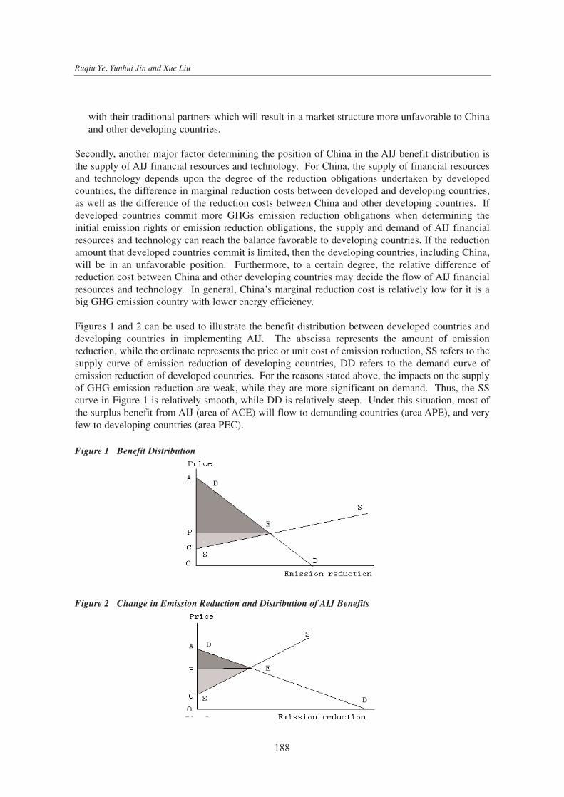
with their traditional partners which will result in a market structure more unfavorable to Chinaand other developing countries.
Secondly, another major factor determining the position of China in the AIJ benefit distribution isthe supply of AIJ financial resources and technology. For China, the supply of financial resourcesand technology depends upon the degree of the reduction obligations undertaken by developedcountries, the difference in marginal reduction costs between developed and developing countries,as well as the difference of the reduction costs between China and other developing countries. Ifdeveloped countries commit more GHGs emission reduction obligations when determining theinitial emission rights or emission reduction obligations, the supply and demand of AIJ financialresources and technology can reach the balance favorable to developing countries. If the reductionamount that developed countries commit is limited, then the developing countries, including China,will be in an unfavorable position. Furthermore, to a certain degree, the relative difference ofreduction cost between China and other developing countries may decide the flow of AIJ financialresources and technology. In general, China’s marginal reduction cost is relatively low for it is abig GHG emission country with lower energy efficiency.
Figures 1 and 2 can be used to illustrate the benefit distribution between developed countries anddeveloping countries in implementing AIJ. The abscissa represents the amount of emissionreduction, while the ordinate represents the price or unit cost of emission reduction, SS refers to thesupply curve of emission reduction of developing countries, DD refers to the demand curve ofemission reduction of developed countries. For the reasons stated above, the impacts on the supplyof GHG emission reduction are weak, while they are more significant on demand. Thus, the SScurve in Figure 1 is relatively smooth, while DD is relatively steep. Under this situation, most ofthe surplus benefit from AIJ (area of ACE) will flow to demanding countries (area APE), and veryfew to developing countries (area PEC).
188
Ruqiu Ye, Yunhui Jin and Xue Liu
Figure 1 Benefit Distribution
Figure 2 Change in Emission Reduction and Distribution of AIJ Benefits
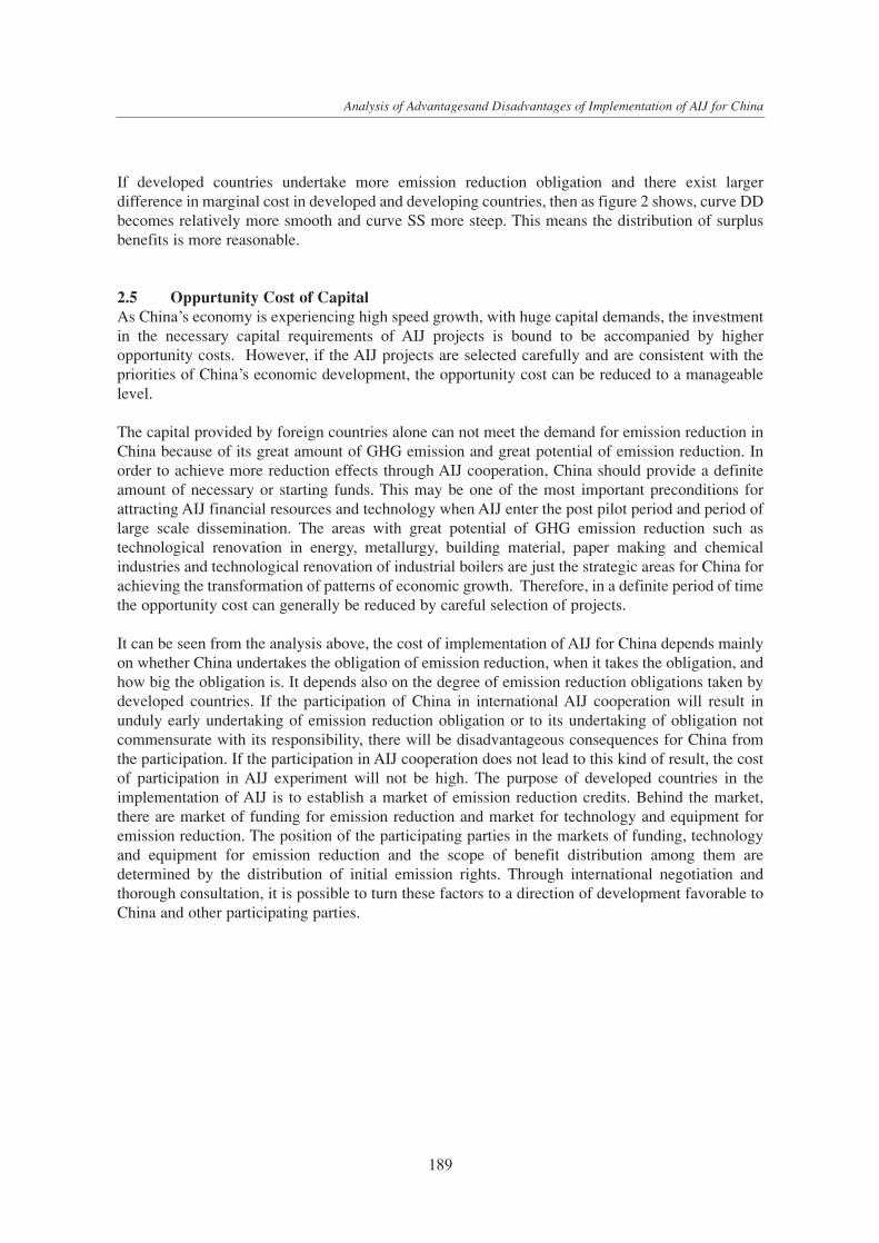
If developed countries undertake more emission reduction obligation and there exist largerdifference in marginal cost in developed and developing countries, then as figure 2 shows, curve DDbecomes relatively more smooth and curve SS more steep. This means the distribution of surplusbenefits is more reasonable.
2.5 Oppurtunity Cost of CapitalAs China’s economy is experiencing high speed growth, with huge capital demands, the investmentin the necessary capital requirements of AIJ projects is bound to be accompanied by higheropportunity costs. However, if the AIJ projects are selected carefully and are consistent with thepriorities of China’s economic development, the opportunity cost can be reduced to a manageablelevel.
The capital provided by foreign countries alone can not meet the demand for emission reduction inChina because of its great amount of GHG emission and great potential of emission reduction. Inorder to achieve more reduction effects through AIJ cooperation, China should provide a definiteamount of necessary or starting funds. This may be one of the most important preconditions forattracting AIJ financial resources and technology when AIJ enter the post pilot period and period oflarge scale dissemination. The areas with great potential of GHG emission reduction such astechnological renovation in energy, metallurgy, building material, paper making and chemicalindustries and technological renovation of industrial boilers are just the strategic areas for China forachieving the transformation of patterns of economic growth. Therefore, in a definite period of timethe opportunity cost can generally be reduced by careful selection of projects.
It can be seen from the analysis above, the cost of implementation of AIJ for China depends mainlyon whether China undertakes the obligation of emission reduction, when it takes the obligation, andhow big the obligation is. It depends also on the degree of emission reduction obligations taken bydeveloped countries. If the participation of China in international AIJ cooperation will result inunduly early undertaking of emission reduction obligation or to its undertaking of obligation notcommensurate with its responsibility, there will be disadvantageous consequences for China fromthe participation. If the participation in AIJ cooperation does not lead to this kind of result, the costof participation in AIJ experiment will not be high. The purpose of developed countries in theimplementation of AIJ is to establish a market of emission reduction credits. Behind the market,there are market of funding for emission reduction and market for technology and equipment foremission reduction. The position of the participating parties in the markets of funding, technologyand equipment for emission reduction and the scope of benefit distribution among them aredetermined by the distribution of initial emission rights. Through international negotiation andthorough consultation, it is possible to turn these factors to a direction of development favorable toChina and other participating parties.
189
Analysis of Advantagesand Disadvantages of Implementation of AIJ for China
3. Analysis of the potential Benefit for China’s Involvement in the AIJInternational Cooperation
International cooperation in AIJ can bring to China direct as well as indirect benefits.
3.1 Direct Benefits from Participation in International Cooperation in AIJ1) China can obtain advanced and appropriate environmental technologyAt present, China is making great efforts to realize the goals of environmental protection, energyconservation and economic growth. Sometimes, there are conflicts between the goals of economicgrowth and environmental protection and energy conservation. Introduction of environmentaltechnologies , especially cleaner production technologies can play an important role in harmonizingthese goals. Participation in international cooperation in AIJ with careful selection of cooperationpartners can help China to obtain advanced and appropriate environmental technologies and topromote sustainable development in China.
2) China can obtain funds necessary for pollution control and GHGs emission reduction.China is still a developing country conducting at present large scale environmental investment..However, it is faced with constraints of economic capability and high opportunity costs. Throughparticipation in international cooperation in AIJ, China can obtain additional funds. This will helpto mitigate the insufficiency of domestic capital and promote the harmonization of economicdevelopment and environmental protection.
It should be noted, that the amount of funds which can be brought to China through internationalcooperation in AIJ depends on the number and scale of AIJ projects. However, the amount oftechnologies which China can obtain depends not only on the number of projects, but more onwhether it is possible to set up a mechanism under the framework of AIJ favorable to the diffusion ofenvironmental technology. In fact, whether AIJ can become an effective mechanism for solving globalenvironmental problems depends in a large extent on whether it is possible to solve the problem ofintellectual property right under the framework of AIJ. This is because the number of AIJ projects islimited no matter in the pilot phase or in the phase of implementation. However, the influence ofdiffusion of environmental technology is hardly possible to estimate. The following analysis ofindirect benefits from international cooperation in AIJ for China was based in a great extent on theassumption of existence of a mechanism favorable for the diffusion environmental technology.
3.2 Indirect Benefits from International Cooperation in AIJ1) China can obtain benefits from the improvement of global environmentIn the sense of total amount of emission, China is one of the countries in the world emitting greatamount of GHGs. If China can take part in AIJ international cooperation in a large scale and gainsignificant effects of emission reduction, it will help to prevent the tendency of degradation and topromote the improvement of the global environment. At the same time, China is naturally thebeneficiary of global environmental improvement. According to the estimate of SamuelFrankhauser (see Table 1), when the CO2 concentration reaches the level of double of that in 1988,the greenhouse effect might cause China great loss accounting for 4.7% of its GNP (the worldaverage level is 1.4%). The estimated loss of China ranks among the top of major countries or groupof countries. China will obviously be the major victimized country of global environmentaldegradation. China will gain great benefits if the global environment is improved.
190
Ruqiu Ye, Yunhui Jin and Xue Liu

2) China can get the benefits of improvements of local environment in China.The local environmental pollution has been becoming more serious as China’s economy has grownquickly in recent years. Table 2 lists the emission and index of increase of major pollutants in Chinafrom 1985-1994.
Table 2 shows the amount of waste gas emission increased by 21% from 1985-1994. If 1986 istaken as the base year, the increase will be 63%. The total amount of SO2 emission is great andincreased by 38% in ten years.. Although the discharge of industrial waste water decreased in certainextent and the emission of industrial dust decreased by about 50%, the total amount of waste is stilllarge. This has caused environmental problems in some areas. It is estimated that by adoptingcleaner production technologies, the current wastes emission can be reduced by about 50%.Therefore, the involvement of China in international cooperation in AIJ can not only reduce GHGemission bringing about global environmental benefits, but also can be helpful to mitigate and solvethe local environmental problems in China.
191
Analysis of Advantagesand Disadvantages of Implementation of AIJ for China
Table 1 Estimated Loss in Percentage of GNP Caused by Greenhouse Effect(CO2 concentration = 2x CO2 concentration in 1988)
Region % of GNP
EU 1.4 USA 1.3 Other OECD 1.4 Former USSR 0.7 China 4.7 Rest of the world 2.0 OECD 1.3 Non OECD 1.6 World 1.4
Source: Samuel Fankhauser: Valuing Climate Change: The Economics of The Greenhouse Effect (London Earthscan1995) p55, Table 3.16
Table 2 The Emission and Index of Increase of Industrial Waste Gas, Waste Water, Dust and SO2(1985 - 1994)
Year Waste gas SO2 Industrial waste Industrial dustBillion cubic 10,000 TONS water 10,000 tons
meters 10,000 tons
Amount Index Amount Index Amount Index Amount Index
1985 93,970 1.00 1,325 1.00 2,574,009 1.00 1,305 1.00 1986 69,679 0.74 1,250 1.01 2,602,380 1.01 1,075 0.82 1987 77,275 0.82 1,412 1.07 2,637,531 1.02 1,004 0.77 1988 82,380 0.88 1,523 1.15 2,683,886 1.04 1,125 0.86 1989 83,065 0.88 1,565 1.18 2,520,945 0.98 840 0.64 1990 85,380 0.91 1,494 1.13 2,486,861 0.97 781 0.60 1991 101,416 1.08 1,622 1.22 2,356,608 0.92 579 0.44 1992 104,787 1.12 1,685 1.27 2,338,534 0.91 576 0.44 1993 109,604 1.18 1,795 1.35 2,194,919 0.85 617 0.47 1994 11363 1.21 1,825 1.38 2,155,111 0.84 583 0.45
Source: China’s Statistics Year Book, from 1986-1995

3) It helps China to promote the strategic transformation of economic growth mode China had been maintaining its economic growth by extensive production. This traditional mode ofeconomic growth had played a role in eradication of poverty and improving living standard of thepeople. However, it also brought about a series of problems such as:
• the vicious circle of high input, high energy consumption, high speed, low output, low benefits
• waste of capital, raw materials and energy, resulting in the shortage of them
• putting emphasis on expansion of scale, ignoring technological innovation and development,which resulted in slow progress of technology, outdated production equipment, weakinternational competitiveness of the Chinese industries
• Unreasonable economic structure The inflation of investment and inflation of consumption occurring in the time of economic growthoften disturbed the process of optimization of the industrial structure and the structure of enterpriseorganization.
Obviously, such growth pattern is not a sustainable one. Therefore, the Chinese government hasdecided to set the transformation of growth pattern as a strategic priority. The central point oftransformation is to improve the efficiency of resource utilization, which is consistent with thestrategic objective of GHG emission reduction. International cooperation in AIJ can be an importantway for China to introduce efficient and clean technology, to improve the efficiency of resourceutilization, and to achieve the goal of transformation of economic growth mode.
4) It helps China to improve energy utilization efficiency Like other developing countries, China has made economic development the first priority. But theshortage of energy has become the bottleneck constraining China’s economic development. It hasbeen predicted that China’s energy demand will reach 1600-1700 million tons of standard coal bythe year 2000. In recent years, China faced a shortage of 20-30 million tons of coal, 10 million tonsof petroleum, and 70 billion kWh of electricity. The gap between the current and potentialproduction capacity of China’s industrial manufacturing sectors has widened because of theshortage of energy and transportation capacity and the aggravation of pollution. It was estimatedthat the loss caused by the shortage of energy is 20-60 times the value of the energy. The shortageof every 100 million tons of coal results in a loss of 100 billion yuan. (Binxian Kui, 1996)
The energy utilization efficiency in China is low. In 1992, the amount of energy consumed on$10,000 of GDP in China was 24,950 tons of standard coal, which was 2.86 times that of India, 5.45times that of the U.S.A., 14.33 of Japan, and 10.86 of Germany. It was estimated that the energyconservation potential in China is 300 million tons of standard coal (Jingshui Sun, 1996). Althoughthe development of energy conservation technology in China has made good progress, there is stilla large gap compared with international levels.
The future economic growth of China will be constrained by the supply of energy. While greatenergy conservation potentials exist, China lacks the technology for conserving energy. Under sucha situation, introducing, digesting, and diffusing clean and efficient technology will be a realisticand favorable choice for China. The implementation of AIJ may be one of the proper ways tointroduce foreign advanced energy conservation technologies at reasonable costs.
192
Ruqiu Ye, Yunhui Jin and Xue Liu

5) It helps China to promoting the development of hydropower and nuclear power.The industrial sector accounts for nearly three quarters of China’s CO2 emission from energyconsumption. Within the five largest energy consuming industries, electricity generation ranks first.Almost 3/4 of the total electricity generated in China come from coal fired power plants. For thepurpose reducing GHG emission, more investments in electricity generating facilities of large scaleand high efficiency are required. However, the improvement of the structure of electricitygeneration through the increase of the proportion of hydro and nuclear electricity is also animportant way.
It is estimated that China has the largest hydropower resources in the world. It has potentialhydropower resources of about 378 GW or an annual electricity generation of 1920 TWh. However,the total installed capacity of hydroelectricity generation accounts only for 9.5% of the totalpotential capacity in China, which is much lower than that of the developed countries, and lowerthan that of Brazil, India and other developing countries. (See Table 3)
Currently there are 2 nuclear power plants in commercial operation in China. The development ofnuclear power has successfully gone through the initial stage. There is a great potential in the futuredevelopment of nuclear electricity in China.
The abundant hydropower resources as well as the great potential for developing nuclear powerprovide the possibility for China to change the energy structure and reduce GHG emission. Theintroduction of funds and technology through participation in international cooperation in AIJ willhelp to turn this possibility into reality.
According to the above discussion, we believed the introduction of environmental technology andfunds through cooperation in AIJ is consistent with the strategic objectives of China in pursuingsustainable development and the transformation of the mode of economic growth. The gain ofpotential benefits is definite. If all parties concerned take the common but differentiated
193
Analysis of Advantagesand Disadvantages of Implementation of AIJ for China
Table 3 The Hydropower Exploitation in Selected Countries
Capacity Electricity Generation
Country Installed Potential I/P ratio Current Potential C/P ratio(GW) (GW) (%) (TWh) (TWh) (%)
USA 90.10 147.25 61.2 279.8 457.1 61.2 Former USSR 64.98 315.73 20.6 223.3 1420.0 15.7 Canada 59.19 163.23 36.3 293.1 593.0 49.4 Brazil 48.75 213.00 22.9 213.4 1194.9 17.9 Japan 37.48 88.0 130.5 67.4 China 36.04 378.53 9.5 126.3 1923.3 6.6 Norway 26.60 121.6 172.0 70.7 France 24.70 69.6 72.0 96.6 Italy 19.00 31.1 60.0 47.8 India 18.34 84.00 21.8 57.8 450.0 12.8 Spain 16.70 25.7 65.6 39.2 Sweden 16.40 71.5 99.0 72.2 Swiss 11.60 30.7 41.0 74.9 Australia 10.90 32.5 53.7 60.5
Source: World Energy Herald, No.13, 1992. (Adjusted, from ZhongXiang Zhang (1996))

responsibilities in accordance with the principles of FCCC and the developing countries areprovided with sufficient “ecological space” necessary for their sustainable development, there willbe more advantages than disadvantages for China’s participation in international cooperation in AIJ.
4. Basic and Prerequisite of China’s participation in International Coopreration of AIJ
GHG reduction is not a game with no winners. Obviously, all parties concerned have a basis ofcommon interests. These are global and regional environmental benefits and many other additionalbenefits brought about by GHG reduction. Therefore, detailed analysis of interests and positions ofall parties and the possibilities and constraints of their strategic choices, and on this basis to findways to mitigate and eliminate conflicts may result in a win-win situation.
4.1 Equity considerationsSharing of environmental responsibilities and obligations on an equitable basis is the prerequisite ofChinas participation in AIJ cooperation. Equity is the key of success of AIJ. Sources of funds,monitoring of projects, distribution of benefits and other aspects of AIJ should be based on theprinciples of environmental equity. Environmental equity among countries will play more and moreimportant role in distribution obligations for resources protection and in bearing the costs ofprevention of environmental pollution and other environmental hazards. Moreover, whileconsidering environmental equity among countries, not only the issue of equity among the presentgeneration of different countries but also the issue of intergenerational equity should be taken intoaccount.
In order that China plays greater role in international cooperation of AIJ, common understanding inthe following aspects is needed.
1) Developed countries are mainly responsible for the degradation of the world environment.Relevant studies show, the amount of carbon dioxide emitted from burning of fossil fuels from 1860to 1949 was 187 billion tons and 55.9 billion tons from 1950 to 1989, of which more than 80% wereemitted by developed countries. At present, the amount of carbon dioxide emitted from burning offossil fuels by developed countries account for about 60% of the total emission amount in the world(Ekins 1995). Although we consider, that the result of the study may underestimate theenvironmental responsibility of developed countries, it still shows that developed countries aremainly responsible for the degradation of the world environment.
2) For the control of degradation of the global environment, countries have common butdifferentiated responsibilities.
It is the capital and technologies accumulated in the previous generations through high consumptionof resources and high emissions of pollutants, that the residents in developed countries can enjoythe present economic achievements and high standard of living. At the same time they should alsoinherit the corresponding environmental responsibilities. The implication of Intergenerationalequity should not be limited only to the equity between the present and future generations, theproblems of distribution of historical responsibilities should also be taken into account.
194
Ruqiu Ye, Yunhui Jin and Xue Liu

3) China and other developing countries are the major sufferers of the environmental degradation.Firstly, As one of the developing countries, China shares the negative external economicconsequence, like the greenhouse effects, of the economic growth of developed countries. This wasshown by the study of Samuel Frankhauser. It can be seen from Table 1, the losses suffered by Chinafrom the greenhouse effects are higher than the world average by 3.36 times. The percentage oflosses in GDP suffered by developing countries is also obviously higher than the world average.Secondly, the development mode of developed countries in the past has resulted in the accumulationof the amounts of GHGs which already exceeded the self-purification capability of the environment.Any new increase of emission will lead to the accelerated increase of environmental costs.Therefore, the choice of development strategy for China and other developing countries is greatlyconstrained.
4) China should not commit to the obligation of GHGs emission reduction that is not commensuratewith its responsibilities and capabilities.
China is one of the countries which emit large amount of GHGs. The amount of carbon dioxideemission of China now accounts for about 11% of the total emission of the world. Nevertheless, theper capita emission of China is very low. For China, sustainable development is the only choice itshould make. However, quite a significant number of technologies of sustainable development canbe developed only when a countrys integrated economic and technical power reaches a definitestage of development. The replacement of fuels is constrained also by the resource andtechnological conditions. The transformation of economic structure needs a long time of period andis not feasible in a short time. Therefore, if China takes the obligation of larger emission reductionbut could not obtain cleaner technologies from developed countries with reasonable prices, thesocial and economic development of China will inevitably be affected seriously.
5) The return from environmental investment for developed countries is higher than for developingcountries. Therefore, developed countries have the responsibilities to support the environmentalcontrol in developing countries.
Countries with different levels of development have different demands for environmental qualityand also different rates of return from environmental investments.
Firstly, for people living in different countries and regions, the environment always has thefollowing functions:
• Contribution of good environment to good quality of life. Good environment is a resource ofcomfort and is enjoyed by human as important constituents of nice scenery and leisure.
• Negative influence of poor environment on quality of life. Poor environment exerts pressure onhuman and affects human health, and further affects the enjoyment of life and labor capability ofhuman.
• Direct contribution of environmental and related industries to development and economicgrowth. Investment in environmental protection and provision of resources of comfort can createbenefit and increase employment.
• Direct contribution of environmental resources to economic activities. For economic activities,the natural environment not only provides raw materials and energy in the form of petroleum,coal, natural gas, fuel woods, minerals etc., but also assimilate wastes and turns them intoresources and regenerate resources.
195
Analysis of Advantagesand Disadvantages of Implementation of AIJ for China
• Contribution to the maintenance of life support system. The ecological functions of oceans,forest, wetlands and other natural environmental systems are now well understood. They playextremely important role in maintaining the life support systems.
Secondly, The effects of environmental quality for countries of different levels of development aredifferent.
The same environmental quality will bring different effects and values to people at different levelsof needs. A. H. Maslow, the American psychologist, divided human needs into five levels:physiological needs, safety needs, social needs including love, belongingness, acceptance andfriendship, esteem needs, and self-actualization needs. Only when the needs of lower level aresatisfied, human will pursue satisfaction of needs of the next higher level. When the needs of lowerlevel have not been satisfied, there will not be driving force for the needs of higher level, or thedriving force will be very weak. Therefore, even if there exist objective conditions for thesatisfaction of needs of higher level, there will be no effects brought about.
Although we can not find a place in the Maslows needs levels for the environmental demand ofhuman, but we can assure, that the first two functions of the environment exceed the level ofphysiological needs and safety needs. In a society where the productivity level is relatively low andthe physiological and safety needs are not fully met, these two functions of the environment onlyhave limited value and importance for this society in comparison with a society with highlydeveloped productivity. Also for this reason, the third function of the environment, the contributionof environmental investment for providing resources of comforts to the increase of employment andthe growth of GDP is negligible. Only the fourth function of the environment has an essentialsignificance for developing countries. However, overexploitation will bring about negativeenvironmental effects.
Thirdly, the return rates of environmental investments are different for developed and developingcountries.
It can be seen from the above discussion, the demand of human for the environmental quality isclosely linked with the level of development. For countries wit different levels of development andincomes, the sensitivity of environmental quality to income is different. For countries of low incomelevel, this kind of demand is insensitive to the change of income. Only when incomes reach arelatively higher level, the elasticity of demand for environmental quality to income will be higherthan one, i.e. this demand is more sensitive to the change of income. For countries of high incomelevel, when the income level rises, the demand for improvement of environmental quality becomesmore urgent, and the improvement of environmental quality will result in more significant effects.This means the return rates of environmental investment will be higher. For countries of low incomelevel, even when there is a rise of the income level, the demand for environmental quality remainsnot very urgent, and the effects brought about by the improvement of environmental quality arelimited. Therefore, the opportunity costs of environmental investment are high, and the return ratesof investment are relatively low. For this reason, developed countries have the responsibility tosupport developing countries for the environmental protection.
In the past, China shared the burdens of the negative external economic effects (like GHG effectsand others) in the process of economic development of developed countries. At present, as the resultof accumulation of GHGs emitted mainly by developed countries, the space of choice ofdevelopment strategy of China is limited. In the future, if China takes the obligation of GHGemission reduction, which is not commensurate with its capability, China will have to import
196
Ruqiu Ye, Yunhui Jin and Xue Liu

expensive emission reduction technologies from developed countries. This will once more putChina in an unfavorable position in international trade which China does not like to face.
4.2. The Feasible Strategic Choice of Developed Countries in Face of Climate Change Caused by the Emission of GHGs.
Facing the hazards of different kinds caused by climate change as the result of anthropogenic GHGemissions and other uncertainties, every country has the following two choices:
• Emission reduction— reduction or elimination of major factors leading to climate change.Because of the externality of the greenhouse effect, the effectiveness of emission reductionactivities depends on the common efforts of many countries. Besides, an internationalmechanism is needed to ensure the effectiveness of the cooperation for the protection of theglobal environment. The costs of emission reduction will depend on the degree of difficulty ofthe following activities in relevant countries: changing the fuel structure, enhancing energyefficiency, transforming economic structure, etc..
• Adaptation— restructuring the social and economic organization to adapt to the changed climateand taking defensive measures to reduce harms caused by climate change. Adaptation is a kindof regional regulative measures which are relatively easy in implementation. The costs ofadaptation include direct costs, for example costs of dams construction to defend from sea levelrise, setting more air conditioners to defend from heat wave attack, readjustment of theagricultural structure to adapt to the change of climatic conditions, etc.. Indirect costs should alsobe included, such as the costs of the spillover of local climatic harms caused by climate change,conflicts caused by fighting for rare and scarce environmental resources, sharp reduction ofbiological diversity, and long term hazards resulted from other irreversible environmentalchanges and others.
It is obvious that adaptation investment and emission reduction investment are not mutuallycomplementary, but are mutually independent and irrelevant. In views of capital scarcity, decisionmakers should make proper choice from the two. Although there exist great uncertainties inestimating the costs of adaptation and the costs of emission reduction, it is certain the costs ofemission reduction the developed countries are willing to pay will not exceed the costs of theiraction of adaptation.
197
Analysis of Advantagesand Disadvantages of Implementation of AIJ for China
References
Ekins, Paul (1996), Economic Implementations and
Decision-Making in the Face of Global Warming,
International Environmental Affairs,Vol..8, No.3, 1996
Summer.
Kui, Binxian (1996), Analysis on Energy Obstacle for
Economic Growth and the Countermeasures, China’s
Soft Sciences, No. 6, 1996.
Sun, Jiangshui (1996), The Urgent Need for Changing the
Economic Growth Pattern From the Compared Study for
China and Abroad, China’s Soft Sciences No. 8, 1996.
Xie, Zhenhua (1996), Cleaner Production — The Best Way
Forward for China’s Industrial Development, World
Environment, No.3, 1996.
Zhang, Zhongxiang (1996), Integrated Economy-Energy-
Environment Policy Analysis: A Case Study for the
People’s Republic of China, Landbouw Universiteit,
Wageningen, 6700 EW Wageningen, The Netherlands,
1996.
198
Ruqiu Ye, Yunhui Jin and Xue Liu

Discussion
ZhongXiang Zhang1
1. Introduction
The paper of Ye et al. (1999) discusses four major issues related to AIJ. The first issue is about thearguments on AIJ. The second issue is about the disadvantages of AIJ for China. The third issue isabout the potential benefits, both direct and indirect, of China’s involvement in AIJ. The fourth issueis about the prerequisites of China’s participation in AIJ. Reading this very interesting papersuggests five questions or issues to me. The first question is about the subject of the paper. Thesecond question is about China’s concern about CDM. The third issue is what China has done so farin limiting its carbon emissions. The fourth issue is what can be expected from China at theinternational climate change negotiations subsequent to Buenos Aires. And the fifth question iswhether combating global climate change is in China’s interest.
2. The Subject: AIJ or CDM?
Acknowledging the strong opposition to the concept of joint implementation in the developingworld, the first Conference of the Parties (COP) to the UNFCCC in Berlin in April 1995 endorseda pilot phase of joint implementation, referred to as “Activities Implemented Jointly” (AIJ) amongAnnex I Parties and, on a voluntary basis, with non-Annex I Parties. During the AIJ pilot phase,emission reductions achieved are not allowed to be credited to current national commitments ofinvestor countries under the UNFCCC. By the time of the UNFCCC’s second synthesis report onAIJ, 95 projects were listed as AIJ projects (UNFCCC, 1998). These projects are located in 24 hostcountries, with Africa hosting only one certified AIJ project. The uneven geographicalrepresentation means that most non-Annex I countries have not experienced an AIJ project withintheir own countries and thus provides insufficient details to draw conclusions. This leads to thedecision 6/CP.4 at the fourth COP to the UNFCCC held in November 1998, Buenos Aires, tocontinue the AIJ pilot phase (UNFCCC, 1999). Although more countries might gain experiencefrom a new round of AIJ projects, however, the future of AIJ is likely to be limited. This is partlybecause of lack of adequate incentives for the private sector participation in AIJ project financing.It is partly because of the adoption of the Buenos Aires Plan of Action, an ambitious two-year workprogramme intended to make the Kyoto Protocol operative (UNFCCC, 1999). According to thePlan, decisions on rules governing cooperative implementation mechanisms are to be made in theyear 2000 at the latest. With the work programme in place, attention has since focused on how cleandevelopment mechanism (CDM), JI and emissions trading would work, with priority being given toCDM. Therefore, it is generally acknowledged that the interest of potential investors in project-based cooperative mechanisms is likely to focus on CDM and JI rather than AIJ.
199
Analysis of Advantagesand Disadvantages of Implementation of AIJ for China
1 The views expressed here are those of the author. The author bears sole responsibility for any errors and omissions that may remain.
The paper of Ye et al. (1999) addresses a variety of concerns regarding to AIJ. However, mach ofthe discussion is related to CDM rather than AIJ. Against the above background, I suggest that thetitle of the paper should indicate that the subject is CDM. Accordingly, the main text should beadjusted to enrich the policy relevance.
3. China’s Concerns about CDM
CDM is an innovative mechanism built into the Kyoto Protocol. While many Annex I countries haveput and continue to put pressure on developing countries to take on emissions limitationcommitments, CDM so far is the only mechanism with an authentic global reach. If designedappropriately, CDM could prove to be a win-win-win mechanism.
• First, CDM could provide an opportunity for developing countries to get increased access tomore advanced energy efficiency and pollution control technologies and additional funding andcould thus accelerate their future development along a more sustainable path.
• Second, it will help Annex I countries to meet their Kyoto commitments at a lower overall costthan would otherwise have been the case.
• Third, CDM enhances international cooperation in combating global climate change and thus isbeneficial to the global environment, as well.
It seems that developing countries prove somewhat more receptive to CDM than to the originalconcept of joint implementation. However, they have still expressed the fear that:
• They would face possible exploitation due to lack of capacity to negotiate fair contracts withCDM investors from Annex I countries.
• All their low-cost abatement options would be used up, leaving them to face only high-costoptions if they would be subsequently required to reduce their own emissions.
• The OECD countries would redefine existing development aid projects as CDM projects, andreduce their aid budgets accordingly. Small developing countries, in Africa in particular, fear thatCDM would tend to shift the OECD countries’ attention towards those developing countries withlarge economies and greenhouse gas emissions.
• Developed countries may use CDM to interfere their internal affairs, given that theimplementation of CDM projects across national borders would touch on the issue of nationalsovereignty.
As a developing country, China shares these general views. But, in my view, there are other specificconcerns that lead to China having taken a cautious approach to CDM.
First, China and India insist that before CDM commences, the entitlements of both developed anddeveloping countries have to be defined (Sharma, 1998).
Second, CDM could lead to attempts to draw developing countries into unduly early agreeing tosomething that could be interpreted as new commitments. Closely related to this, there is a particularconcern about country-wide baselines that aim to address the leakage problems associated withproject baselines, because of their possible links to voluntary or binding commitments. So, in orderto protect the longer-term interests of developing countries, it must be absolutely clear from theoutset that such baselines, if any, are only for the purpose of reckoning the CDM credits during theagreed periods, without prejudice to future divisions of mitigation responsibilities.
200
ZhongXiang Zhang

Third, although the sustainable development objective of CDM makes it attractive to developingcountries, there is a tendency that CDM would serve the only purpose of assisting Annex I countriesin meeting their commitments. Much of the discussion on the CDM to date has focused on technicalissues, but its sustainable development objective has not received as much attention. This to a largeextent explains why CDM does not trigger much more interests from the developing world thanwhat was thought to be the case. If CDM were only beneficial to Annex I countries, CDM could notbe sustained.
In order to facilitate the effective developing country participation in the CDM, the sustainabledevelopment objective of the CDM must be addressed. Because the CDM will be eventuallyimplemented through projects, this raises a very important question: how can the objective ofsustainable development be explicitly incorporated into individual CDM projects?
One possible option is to develop a set of operational criteria or indicators against which social,economic and environmental dimensions of individual CDM projects can be measured. They coulddiffer per type of CDM projects. If sustainable development indicators could be defined inoperational terms and be adopted by the parties to the UNFCCC, they provide useful and user-friendly information to guide decisions about whether a proposed CDM project contributes tosustainable development. Another option would be to require the project developers to demonstratehow the CDM project in question is compatible with development priorities of the host country. Itis not enough that CDM projects be not harmful because harmless projects that are unrelated todevelopment priorities divert limited resources away from priority activities and thus involve highopportunity cost for the host country. In my view, no matter what an option to measure sustainabledevelopment is adopted, host developing countries retain the right to decide whether a proposedCDM project is likely to contribute to sustainable development.
4. What Has China Done so far in Limiting its Carbon Emissions?
The paper of Ye et al. (1999) mentions several times that China should not commit any greenhousegas abatement obligations that are not commensurate with its capabilities. But it does not spell outwhat a level of commitment could be acceptable to China. At present, China contributes 13.5% ofglobal CO2 emissions. Its share in global CO2 emissions is expected to exceed that of the US by2020, if the current trend of economic development in China continues (World Bank, 1994).Therefore, it is not surprising that the role of China is a perennial issue at the international climatechange negotiations. Before going into elaborate efforts and commitments that can be expected fromChina, I like to address what China has done so far in terms of limiting its carbon emissions. Thereason why I pay attention to this issue is that significant contribution China has made to reducingglobal CO2 emissions has been too little appreciated.
With more than 1.2 billion people, China is home to about 21.5% of the world’s population (seeTable 1) and has a large and rapidly growing economy, making the country an important player onthe world’s stage. Since launching its open-door policy and economic reform in late 1978, Chinahas experienced spectacular economic growth, with its gross domestic product (GDP) growing atthe average annual rate of about 10% over the period 1978-1997. Along with the rapid economicdevelopment, energy consumption rose from 571.4 million tons of coal equivalent (Mtce) in 1978to 1440.0 Mtce in 1997 (State Statistical Bureau, 1998).
201
Analysis of Advantagesand Disadvantages of Implementation of AIJ for China

Accompanying the growth in fossil fuel use, China’s CO2 emissions have grown rapidly. As shownin Figure 1, the total CO2 emissions in China rose from 358.60 million tons of carbon (MtC) in 1980to 847.25 MtC in 1997, with an average annual growth rate of 5.2%. This ranks China as the world’ssecond largest CO2 emitter only behind the US, according to the World Energy Council (see Table1). But on a per capita basis, China’s CO2 emissions of 0.685 tC in 1997 were very low, only abouthalf the world average (Zhang, 1999).
The breakdown of CO2 emissions by fuel is shown in Figure 1. Because coal has accounted forabout 75% of the total energy consumption over the past years, it is not surprising that coalpredominates, accounting for 81.3% of the total emissions in 1997. This share has remained almostunchanged over the past two decades
Table 2 shows the historical contribution of inter-fuel switching, energy conservation, economicgrowth, and population expansion to CO2 emissions in China over the period 1980-1997. The dataused to obtain the results in Table 2 are plotted in Figure 2, after normalization to the year 1980. Theresults in Table 2 and Figure 2 clearly indicate the relative importance of each factor in terms of its
202
ZhongXiang Zhang
Table 1 Shares of Global CO2 Emissions and World Population, 1996
Share of global CO2 emissions (%) Share of the world population (%)
USA 25.0 4.7EU-15 14.7 6.5China 13.5 21.5CIS Republics 10.2 5.0Japan 5.6 2.2India 3.6 16.3Canada 2.1 0.5Australia 1.3 0.3
Source: Jefferson (1997).
Figure 1 China’s CO2 Emissions by Fuel
Source: Zhang (1999).
0
100
200
300
400
500
600
700
800
900
1980 1990 1997
CO
2 E
mis
sion
s (M
tC)
Natural gas
Oil
Coal

contribution to CO2 emissions growth in China. Given that China has been the most rapidlyexpanding economy over the past 17 years, it is not surprising that economic growth measured inper capita GDP was overwhelming. This factor alone resulted in an increase of 799.13 MtC. Duringthe corresponding period, through its strict family planning programmes, China experienced a verylow rate of population growth in comparison with other countries at China’s income level, which inturn contributed to a smaller increase in China’s CO2 emissions than would otherwise have been thecase.2 As a result, population expansion was responsible for an increase of 128.39 MtC, an increasein emissions considered to be modest given its population size. Also, the change in fossil fuel mixcontributed to an increase in emissions (3.93 MtC), but its role was very limited because the shareof coal use in total commercial energy consumption increased only slightly during the period.
By contrast, a reduction in energy intensity tended to push CO2 emissions down. Since the early1980s, the Chinese government has been placing great emphasis on energy conservation and hasformulated and implemented approximately 30 energy conservation laws concerning theadministrative, legislative, economic and technological aspects of energy conservation. After yearsof preparation, China’s Energy Conservation Law was enacted on 1 November 1997 and came intoforce on 1 January 1998. In order to efficiently use energy, China has significantly reduced subsidiesfor energy consumption, with coal subsidy rates falling from 61% in 1984 to 37% in 1990 and to29% in 1995, and petroleum subsidy rates falling from 55% in 1990 to 2% in 1995 (Kosmo, 1987;World Bank, 1997a). Currently, coal prices are largely decided by the market and vary significantlydepending on the destination of the coal.3 Energy pricing reforms may have already proceeded tothe point where the bottlenecks to more adoption of efficiency measures have less to do with energyprices than other factors (Sinton et al., 1998). Along with the economic reforms that, among otherachievements, have spurred investment in more energy efficient production technologies, theChinese government has also played a crucial role both in promoting a shift of economic structuretowards less energy-intensive services (see Table 3) and a shift of product mix towards high value-added products, and in encouraging imports of energy-intensive products.4 Furthermore, effortshave been made towards implementing nationwide energy conservation programmes. For example,state capital construction loans for efficiency are at an interest rate of 30% lower than commercialloans, and state technological renovation loans for efficiency are with 50% of the interest subsidized
203
Analysis of Advantagesand Disadvantages of Implementation of AIJ for China
Table 2 Breakdown of the Contributions to CO2 Emissions Growth in China, 1980-1997 (MtC)a
Due to change Due to Due to Due to Due to Total changein fossil fuel penetration change economic population in CO2carbon intensity of carbon in energy growth expansion emissions
free fuel intensity
+3.93 -10.48 -432.32 +799.13 +128.39 +488.65
a A positive sign indicates an increase; A negative sign indicates a decline.Source: Zhang (1999).
2 During the period 1980-1997, the annual average growth rate of population in China was 1.33%. In contrast, the corresponding figurefor low-income economies (excluding China) between 1980 and 1995 was 2.35%, and the world average was 1.66% (World Bank,1997c).
3 For example, the mine-mouth price of Datong mixed coal was 128 yuan per ton in June 1994. The same coal retained for 230 yuan perton in Shanghai, 262 yuan per ton in Nanjing, 280 yuan per ton in Guangzhou, and 340 yuan per ton in Xiamen (SETC, 1996).
4 About 10% of the total energy savings during the period 1981-1988 were attributed to imports of energy-intensive products (Zhang,1997).

(Sinton et al., 1998). The creation of over 200 energy conservation technology service centersthroughout the country, which have worked most closely with the end-users of the efficienttechnologies, devices and practices that the government sought to promote, has been extremelyvaluable. In power industry, efforts have been made towards developing large-size coal-fired powerplants. In 1987, only 11 power stations had an unit capacity of 1 gigawatt (GW) and above. Thecombined capacity of these power stations was about 15 GW, accounting for one-seventh of thenation’s total. By 1994, there were 34 power stations having an unit capacity of 1 GW and above,with a combined capacity of 43 GW, accounting for 21.4% of the nation’s total (SETC, 1996). Inthe meantime, the share of generating units having a capacity of 100 MW and above increased from32.5% in 1984 to 57.2% in 1994 (MOEP, 1985; SETC, 1996). Along with these large unitscommissioned into operation, the average generation efficiency of thermal power increased from28.5% in 1984 to 29.7% in 1994. Given the sheer size of the Chinese power industry, even this smallefficiency improvements translate into large coal savings when multiplied by tens of GW ofcapacity installed.
Figure 2 Contribution to CO2 Emissions in China, 1980-1997a
a C = The amount of CO2 emissions; FEC = Total carbon-based fossil fuel consumption; TEC = Totalcommercial energy consumption; GDP = Gross Domestic Product; and POP = Population.Source: Zhang (1999).
204
ZhongXiang Zhang
0
50
100
150
200
250
300
350
400
450
1980
1981
1982
1983
1984
1985
1986
1987
1988
1989
1990
1991
1992
1993
1994
1995
1996
1997
Index(1980=100) POP
C
GDP/POP
TEC/GDP
FEC/TEC
C/FEC

Clearly, it is by implementing these policies and measures that great progress in decoupling China’sGDP growth from energy consumption has been made, with an annual growth of 10.06% for theformer but only 5.26% for the latter during the period 1980-1997. This achievement corresponds toan income elasticity of energy consumption of 0.52 and to an annual saving rate of 4.37%.5 Giventhe fact that most developing countries at China’s income level have the income elasticity of energyconsumption well above one (see Table 4), this makes China’s achievement unique in thedeveloping world.6 As a result, a reduction of 432.32 MtC was achieved. In other words, withoutthe above policies and measures towards energy conservation, China’s CO2 emissions in 1997would have been 432.32 MtC higher, or more than 50% higher, than its actual emissions.
In addition to energy conservation, the penetration of carbon-free fuels contributed to a smallreduction in CO2 emissions (-10.48 MtC). This is mainly due to the underdevelopment ofhydropower, and partly because the development of nuclear power in China is still at the initial start-up stage.
205
Analysis of Advantagesand Disadvantages of Implementation of AIJ for China
Table 3 The Composition of GDP in China, Japan and the US (percentage of GDP)
China Japan United States 1980 1990 1997 1995 1995
Agriculture 30.1 27.1 18.7 2 2Industry 48.5 41.6 49.2 38 26Services 21.4 31.3 32.1 60 72
Sources: State Statistical Bureau (1998); World Bank (1997c).
Table 4 Growth Rates of GDP and Energy Consumption, and the Income Elasticity of EnergyConsumption among Different Economies, 1980-1994
Annual growth Annual growth Income elasticity of GDP (%) of energy of energy
consumption (%) consumption
Low-income economies * 2.8 4.7 1.66China 11.0 4.5 0.41
Upper-middle-income economies 2.5 3.9 1.56High-income economies 2.8 1.1 0.39
* Excluding China.Source: Calculated based on data from the World Bank (1996).
5 The income elasticity of energy consumption is defined as the change in energy consumption divided by the change in economic growth.
6 As shown in Table 4, the income elasticity of energy consumption in China is quite low by international standards. In addition to energyconservation, there are other two possible explanations for this. First, the growth of energy consumption is underestimated relative to theGDP growth. Second, quantitative restrictions have kept energy consumption from rising as would otherwise have occurred. Drawing onthe analysis of rationing by Neary and Roberts (1980), the quantitative restrictions act like an implicit energy tax levied at rates varyingwith use and fuel. Generally speaking, households face a higher implicit tax than industrial users, and oil and natural gas are taxed at ahigher rate than coal.
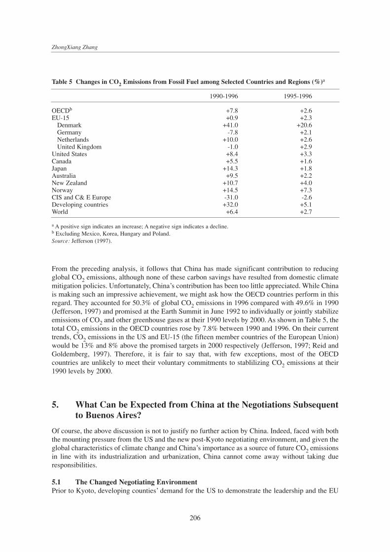
From the preceding analysis, it follows that China has made significant contribution to reducingglobal CO2 emissions, although none of these carbon savings have resulted from domestic climatemitigation policies. Unfortunately, China’s contribution has been too little appreciated. While Chinais making such an impressive achievement, we might ask how the OECD countries perform in thisregard. They accounted for 50.3% of global CO2 emissions in 1996 compared with 49.6% in 1990(Jefferson, 1997) and promised at the Earth Summit in June 1992 to individually or jointly stabilizeemissions of CO2 and other greenhouse gases at their 1990 levels by 2000. As shown in Table 5, thetotal CO2 emissions in the OECD countries rose by 7.8% between 1990 and 1996. On their currenttrends, CO2 emissions in the US and EU-15 (the fifteen member countries of the European Union)would be 13% and 8% above the promised targets in 2000 respectively (Jefferson, 1997; Reid andGoldemberg, 1997). Therefore, it is fair to say that, with few exceptions, most of the OECDcountries are unlikely to meet their voluntary commitments to stablilizing CO2 emissions at their1990 levels by 2000.
5. What Can be Expected from China at the Negotiations Subsequentto Buenos Aires?
Of course, the above discussion is not to justify no further action by China. Indeed, faced with boththe mounting pressure from the US and the new post-Kyoto negotiating environment, and given theglobal characteristics of climate change and China’s importance as a source of future CO2 emissionsin line with its industrialization and urbanization, China cannot come away without taking dueresponsibilities.
5.1 The Changed Negotiating Environment Prior to Kyoto, developing counties’ demand for the US to demonstrate the leadership and the EU
206
ZhongXiang Zhang
Table 5 Changes in CO2 Emissions from Fossil Fuel among Selected Countries and Regions (%)a
1990-1996 1995-1996
OECDb +7.8 +2.6EU-15 +0.9 +2.3
Denmark +41.0 +20.6Germany -7.8 +2.1Netherlands +10.0 +2.6United Kingdom -1.0 +2.9
United States +8.4 +3.3Canada +5.5 +1.6Japan +14.3 +1.8Australia +9.5 +2.2New Zealand +10.7 +4.0Norway +14.5 +7.3CIS and C& E Europe -31.0 -2.6Developing countries +32.0 +5.1World +6.4 +2.7
a A positive sign indicates an increase; A negative sign indicates a decline.b Excluding Mexico, Korea, Hungary and Poland.Source: Jefferson (1997).

proposal for a 15% cut in emissions of a basket of three greenhouse gases below 1990 levels by2010 put collective pressure on the US, which leads the world in greenhouse gas emissions. Nowthe US has made legally binding commitments at Kyoto. The Kyoto target is seen as not enough butyet not unreasonable given that the US economy would not be disrupted unreasonably (King,1998).7 Now the ball is kicked off to China’s court. The US has made it clear that bringing keydeveloping countries, including China, on board has been and will continue to be its focus ofinternational climate change negotiations. According to some US Senators, it will be countries likeChina, India and Mexico that will decide whether the US will ratify the Kyoto Protocol. It istherefore conceivable that the pressure will mount for China to make some kind of commitments atthe negotiations subsequent to Buenos Aires. The world’s media will undoubtedly bring attention toChina’s non-participation, which will be seen as holding up the ratification of the Protocol by theUS Senate and possibly even be blamed for “blowing up” subsequent negotiations aimed at dealingwith developing countries’ commitments.
While preparing for greater and greater pressure from the US, China should take the following non-US factors into account in developing its post-Kyoto climate negotiation strategies.
First, although the group of 77 and China8 managed to block the US proposal for allowing adeveloping country to voluntarily commit to reductions in greenhouse gas emissions at Kyoto, theUS had partial success in weakening the position of the group. As might be expected, the US willcontinue to apply the “divide and rule” tactic by getting at least a few to accept obligations they arenot required to undertake and then putting pressure on the rest of the developing countries to do thesame, exploiting the fact that such developing countries as Argentina have already determined totake on voluntary commitments.9 Given the fact that developing countries are a more diverse andheterogeneous group than the Annex I countries, and that their interests in the climate change debateare heterogeneous and occasionally competing, it might be very difficult to prevent some countriesin the group — particularly those countries with a relatively high per capita income and thatperceive the greatest potential gain from emissions trading — from being drawn into makingcommitments of their own at the negotiations subsequent to Buenos Aires.
Second, after the first commitment period 2008-2012, China will soon surpass the US as the world’slargest greenhouse gas emitter, due mainly to its sheer size of population and partly to its rapidlygrowing economy. While it will still take another couple of decades for cumulative greenhouse gasemissions from China to exceed those of the US, Western media and some US Senators coulddeliberately misguide the general public’s attention and then shift the attack on the US to China.
Third, although in accordance with the principle of common but differentiated responsibilitiesAnnex I countries should take the lead in reducing their greenhouse gas emissions and providing
207
Analysis of Advantagesand Disadvantages of Implementation of AIJ for China
7 As indicated in Table 5, the US CO2 emissions in 1996 were already 8.4% above 1990 levels. To meet the Kyoto commitments requiresthe US to cut its greenhouse gas emissions by up to 30% from its business-as-usual levels during the period 2008-2012. This is nottremendous but not trivial either.
8 As has been the case in the international climate change negotiations, the developing countries express their consensus views as thegroup of 77 and China’s positions. Divergent or dissenting views are then expressed separately, representing either individual countriesor smaller groups, such as the Alliance of Small Island States (AOSIS).
9 At the fourth COP to the UNFCCC held in November 1998, Buenos Aires, the host country, Argentina, proposed the inclusion ofvoluntary commitments from developing countries on the conference agenda. When delegates considered the agenda, a Chinese delegatesaw any discussion on the subject of voluntary commitments from developing countries as a means of destroying the unity of the groupof 77 and China, while a Brazilian negotiator said it was a means of helping some countries to avoid existing commitments rather thanpromoting the UNFCCC (Earth Negotiations Bulletin, 16 November 1998). As a result, the host’s proposal was rejected by the group of77 and China. In the end, during the second week of the fourth COP, Argentina and Kazakstan stepped out from the ranks of the groupof 77 and China and declared that they would undertake a voluntary commitment to abate their greenhouse gas emissions at the fifth COPto the UNFCCC in 1999.

adequate technology transfer and financing to non-Annex I countries, broadening commitments toinclude all countries in the long term is necessary and unavoidable in order to achieve theUNFCCC’s ultimate objective of stabilizing greenhouse gas concentrations in the atmosphere at alevel that would prevent dangerous anthropogenic interference with the climate system.
Under these circumstances, it would be unwise for China just to sit back and let the US define whatis “meaningful participation” from developing countries. It would be also unwise for China simplyto distance itself from attempts to draw developing countries into agreeing to something that couldbe interpreted as new commitments at the negotiations subsequent to Buenos Aires. Doing so wouldonly create negative image and publicity for China, which has been regarded as a “hard liner” at theclimate change negotiations. In the meantime, China should keep watch on the negotiating positionsof such developing countries as Argentina, Costa Rica and South Korean and should not let the fateof the whole South be left at the hands of these relatively high-per-capita-income countries.
5.2 China’s Strategies at the Climate Change Negotiations Subsequent to Buenos AiresFaced with a different situation from that at Kyoto, China should ponder deeply over its strategiesat the international climate change negotiations subsequent to Buenos Aires. On the one hand, Chinashould take much more efforts towards communicating to the industrialized world the substantialcontributions it has already made to limiting greenhouse gas emissions. China has cut its energyconsumption per unit of output in half since 1980, indicating that if the energy intensity were thesame now as that in 1980, China would consume twice as much energy, and produce twice as muchCO2 emissions as it now does. Unfortunately, this achievement is not widely known or appreciatedoutside of China: outsiders know that the Chinese economy is booming, but they are not ascognizant of China’s very impressive improvement in energy efficiency. Therefore, efforts towardseffective communication about what has been achieved in China to the outside world will help tocorrect the distorted picture that had been painted.
On the other hand, while insisting on its legitimate demand for industrialized countries to provideadequate technology transfer and financing, and demanding that emissions targets beyond the firstcommitment period be set for Annex I countries at the subsequent negotiations over new additionaldeveloping countries’ commitments, China could propose and direct negotiations, rather than justreact and respond. In proposing its voluntary efforts and commitments, China should bear in mindthat demanding for the “equal per capita entitlements” is politically unrealistic for the time span weare considering, although it is perfectly justified on grounds that all human beings are born equaland that the atmosphere is a global common. On the other hand, the US demand for imposing a capon China’s future emissions is absolutely unacceptable for China, at least until its per capita incomecatches up with the level of middle-developed countries. For these reasons, I put aside the proposalfor either “equal per capita entitlements” or an absolute cap on national emissions. I envision thefollowing six proposals that could be put on the table as China’s plausible negotiation position,which are each described in the order of their stringentness.
First, China could regard its active participation in CDM as “meaningful participation”. Ifappropriate rules and guidelines for CDM are defined, what then are the potential areas in China’sinterest? It is usually acknowledged that the success of CDM premises an effective understandingof local (host country) development aspirations and the use of CDM to push ahead with efforts toachieve these aspirations. Thus, in order to enhance their possibility of success, there is the need tomake due consideration of local objectives and local conditions in designing the CDM projects.Considering that China is more concerned with local pollutants, such as SO2, NOx and particulatesfrom coal burning, and regards them as its own environmental priorities, it is expected that the most
208
ZhongXiang Zhang

potential areas of interest to China are related to those activities and options aimed at: (1) improv-ing the efficiency of energy use, particularly at energy-intensive energy sectors (for example, ironand steel industry, chemical industry, building materials industry, and power industry) and devices(for example, industrial boilers); (2) pushing efficient use of coal through increasing proportion ofraw coal washed; popularizing domestic use of coal briquette; substitution of direct burning of coalby electricity through development of large-size, high-temperature and high-pressure efficient coal-fired power plants; expanding district heating systems and developing co-generation; increasedpenetration of town gas into urban households; and through development and diffusion of environ-mentally sound coal technologies; (3) speeding up the development of hydropower and nuclearpower; and (4) developing renewables.
Second, just as Article 3.2 of the Kyoto Protocol requires Annex I countries to “have madedemonstrable progress” in achieving their commitments by 2005, China could commit todemonstrable efforts towards slowing its greenhouse gas emissions growth at some point betweenthe first commitment period and 2020. Securing the undefined “demonstrable progress” regardingChina’s efforts is the best option that China should fight for at the international climate changenegotiations subsequent to Buenos Aires.
Third, if the above commitment is not considered “meaningful”, China could go a little further tomake voluntary commitments to specific policies and measures to limit greenhouse gas emissionsat some point between the first commitment period and 2020. Policies and measures might need tobe developed to explicitly demonstrate whether or not China has made adequate efforts. Suchpolicies and measures might include abolishing energy subsidies, improving the efficiency ofenergy use, promoting renewable energies, and increasing the R&D spending on developingenvironmentally sound coal technologies.
China should resort to all means of securing either of the above deals. It could even lobby forsupport from the EU, and therefore put collective pressure on the US.10 If all the attempts proveunsuccessful, China might resort to the last three options.
Fourth, China could make a voluntary commitment to total energy consumption or total greenhousegas emissions per unit of GDP at some point around or beyond 2020. In my view, carbon intensityof the economy is preferred to energy intensity of the economy (i.e., total energy consumption perunit of GDP) because all the efforts towards shifting away from high-carbon energy are awarded bythe former. Such a commitment would still allow China to grow economically while improving theenvironment. It reflects a basic element of the UNFCCC, which has recongnized the developingcountries’ need for further development and economic growth. The industrialized countries,particularly the US, have no reason or right to argue against it. To do so would contradict their claimthat asking China’s involvement in combating global climate change is not intended to limit itscapacity to industrialize, reduce poverty and raise its standards of living. Even if the Chinesegovernment has claimed that China will continue its efforts towards improving energy efficiencyand minimizing further degradation of the environment in any event, it would be wise to propose anexplicit value for carbon intensity of the Chinese economy as a starting point for negotiations. In
209
Analysis of Advantagesand Disadvantages of Implementation of AIJ for China
10 In the run up to Kyoto, the following two points distinguish the EU from the US. In comparison with the US demand for developingcountries to agree to cuts in greenhouse gas emissions in the same timeframe as industrialized countries, the EU has made clear thatdeveloping countries need not to promise at Kyoto to make cuts, although they should be persuaded to do so at a later date. Moreover,by permitting a 30-40% increase in emissions to Greece and Portugal, the EU proposal for international community burden-sharingaccepts that poorer countries should be treated more leniently, whereas the US has been opposed to differentiated emissions targets untilit has to give up its opposition at Kyoto. If Greece and Portugal can have this sort of rise, it would be very difficult for the EU to rejectthe demand from the really poor, that is, developing countries, for a not unreasonable leeway in emissions.

this regard, there is a pressing need for comprehensive analysis and quantification of the economicimplications of climate change for China. For a long time, the Chinese government has claimed thatasking for China to take actions would seriously harm China’s economic development. However,until now, inside of China there has been no single comprehensive study indicating the economiceffects of possible future carbon limits for China, for example, in terms of foregone national income,although along this line there have been some studies done outside of China (e.g., Zhang (1997,1998)). Findings that show that China would be the region hardest hit by carbon limits can help toconvince the world of the Chinese government’s claim. Such information can be used to China’sadvantage in bargaining a possible targeted carbon intensity with other countries, as well.
The fifth option would be for China to voluntarily commit to an emissions cap on a particularsector at some point around or beyond 2020. Taking on such a commitment, although alreadyburdensome for China, could raise the concern about the carbon leakage from the sector to thosesectors whose emissions are not capped.
This leads to the final option that China could offer: a combination of a targeted carbon intensitylevel with an emissions cap on a particular sector at some point around or beyond 2020. This is thebottom line: China can not afford to go beyond it until its per capita income catches up with the levelof middle-developed countries.
It should be pointed out that before legally binding commitments become applicable to Annex Icountries, they have a grace period of 16 years starting from the Earth Summit in June 1992 whenAnnex I countries promised to individually or jointly stabilize emissions of CO2 and othergreenhouse gases at their 1990 levels by the end of this century to the beginning of the firstcommitment period in 2008. Therefore, China could demand a grace period before either of the lastthree commitments becomes legally binding. Even without the precedent for Annex I countries,China’s demand is by no means without foundation. For example, the Montreal Protocol onSubstances that Deplete the Ozone Layer grants developing countries a grace period of 10 years.Moreover, China could insist that accession of developing countries and burden sharing be based onability of pay. As such, a country is expected to take on emissions limitation commitments once itexceeds a threshold level of per capita income. On the one hand, this approach would avoid thecosting negotiations for accession of developing countries on an individual basis. On the other hand,the approach would bind China and other developing countries, thus giving China more clout in thefinal bargaining in determining a threshold level.
6. Combating Global Climate Change Is in China’s Interest
I fully agree with Ye et al. (1999) that China itself will benefit from international cooperation oncombating global climate change. Because economic development remains the priority for China,its climate policy would focus on the so-called win-win strategies. The above efforts andcommitments proposed for China reflect that; they do not go beyond the scope of taking no-cost orlow-cost “no-regrets” actions. Although the last three commitments are more stringent than the firstthree, none of them would be likely to severely jeopardize Chinese economic development. Indeed,taking due responsibilities in combating global climate change should be in China’s interest on thefollowing grounds.
First, because climate-sensitive sectors such as agriculture still account for a much larger proportionof GDP in China than in the developed countries (see Table 3), China is even more vulnerable to
210
ZhongXiang Zhang

climate change than the developed countries. Therefore, a broad commitment to global effortstowards limiting greenhouse gas emissions would reduce the potential damage from climate changein China itself, since after all it is not only the developed countries whose climate will change ifgreenhouse gas emissions are not reduced.
Second, China is scarce in energy, with per capita energy endowments far below the world average(see Table 6). Although energy consumption per unit of output in China has been cut in half since1980, its major industries continue to use energy far more intensively than in industrializedcountries (see Table 7). By making the above commitments, China will be pushed for a moreefficient use of its scarce energy resources.
Third, driven by the threat of further degradation of the environment11 and the harmful economiceffects of energy shortages, China is already determined to push energy conservation and enhancedenergy efficiency in general and more efficient coal usage in particular. Although it is taking suchdrastic domestic efforts on its own, China badly needs assistance and economic and technicalcooperation with the developed countries, because of the huge amounts of capital and technicalexpertise required. In this regard, CDM, if designed appropriately, could provide an opportunity forChina to get increased access to more advanced energy efficiency and pollution control technologiesand additional funding.
From the preceding discussion, it follows that the above efforts and commitments proposed forChina, though aimed at limiting greenhouse gas emissions, will contribute to the reductions in localpollutants and thus will be beneficial to a more sustainable development of the Chinese economy aswell as to the global climate. At the same time, they would give China more leverage at theinternational climate change negotiations subsequent to Buenos Aires.
211
Analysis of Advantagesand Disadvantages of Implementation of AIJ for China
Table 6 Proved Reserves and Utilization Rates of Fossil Fuels in China, 1997
Resources Proved reserves R/P ratioa Per capita proved (years) reservesb
China China World China World
Coal 114.5 billion tons 82 219 95 182% world total 11.1%
Oil 3.3 billion tons 21 41 3 25% world total 2.3%
Natural gas 1.16 trillion cubic meters 52 64 967 25517% world total 0.8%
a R/P ratio stands for the lifetime of proved reserves at 1997 rates of production.b Measured in tons for coal and oil and in cubic meters for natural gas and based on population in 1995.Sources: Calculated based on data from the British Petroleum (1998) and World Bank (1997c).
11 Existing estimates for the economic costs of China’s environmental degradation vary, depending on the comprehensiveness of theestimates. For example, using the measure of willingness to pay, the World Bank (1997b) has estimated that air and water pollution costChina about 8% of its GDP, around $54 billion annually, while Smil (1996) puts China’s environmental damages between 5.5% and 9.8%of its GNP.

212
ZhongXiang Zhang
Table 7 A Comparison of Unit Energy Consumption for Selected Energy-Intensive Users
1980 1994 AdvancedChina China level abroad
Comparable energy consumption per ton of steel (tce/t) 1.30 1.03a 0.6 (Italy)Energy consumption per ton of synthetic ammonia (tce/t) 1.45 1.34a 1.2
Large plants 2.90 2.09 108.4 (Japan)Small plants 206.5 175.3 327 (ex-USSR)
Energy consumption per ton of cement clinker (kgce/t) 448 413 80-85 Net coal consumption of coal-fired plants (gce/kWh) 60-70
Thermal efficiency of industrial boilers (%)
a In 1990.Source: Zhang (1997).
References
British Petroleum (1998), BP Statistical Review of WorldEnergy 1998, London.
Jefferson, M. (1997), Potential Climate Change: CarbonDioxide Emissions 1990-96, World Energy CouncilJournal, pp. 76-82.
King, E. (1998), Spoke as a Representative of Small IslandStates at the Latin American Workshop on NewPartnerships for Sustainable Development: The CleanDevelopment Mechanism under the Kyoto Protocol,28-29 April, Mangaratiba, Brazil.
Kosmo, M. (1987), Money to Burn? The High Costs ofEnergy Subsidies, World Resources Institute,Washington, DC.
MOEP (1985), Electric Power Industry in China 1984-85,Ministry of Electric Power (MOEP), Beijing.
Neary, J.P. and K.W.S. Roberts (1980), The Theory ofHousehold Behaviour under Rationing, EuropeanEconomic Review, Vol. 13, pp. 25-42.
Reid, W. and J. Goldemberg (1997), Are DevelopingCountries Already Doing As Much As IndustrialisedCountries to Slow Climate Change?, Climate Notes,World Resources Institute, Washington, DC.
SETC (1996), China Energy Annual Review, StateEconomic and Trade Commission (SETC), Beijing.
Sharma, A. (1998), Climate No Headway, Down to Earth,Vol. 7, No. 14, Centre for Science and Environment,New Delhi.
Sinton, J.E., Levine, M.D. and Q.Y. Wang (1998), EnergyEfficiency in China: Accomplishments andChallenges, Energy Policy, Vol. 26, No. 11, pp. 813-829.
Smil, V. (1996), Environmental Problems in China:Estimates of Economic Costs, East-West Center,Honolulu.
State Statistical Bureau (1998), A Statistical Survey ofChina 1998, State Statistical Publishing House,Beijing.
UNFCCC (1998), Review of the Implementation ofcommitments and of other Provisions of theConvention. Activities Implemented Jointly: Reviewof Progress under the Pilot Phase (Decision 5/CP.1),Second Synthesis Report on Activities Implemented,United Nations Framework Convention on ClimateChange (UNFCCC), FCCC/CP/1998/2, Bonn.
UNFCCC (1999), Part Two of the Report of theConference of the Parties on its Fourth Session, Held atBuenos Aires from 2 to 14 November 1998: ActionTaken by the Conference of the Parties on its FourthSession, United Nations Framework Convention onClimate Change (UNFCCC),FCCC/CP/1998/16/Add.1, Bonn.
World Bank (1994), China: Issues and Options inGreenhouse Gas Emissions Control, Washington, DC.
World Bank (1996), World Development Report 1996,Oxford University Press, New York.
World Bank (1997a), Expanding the Measure of Wealth:Indicators of Environmentally SustainableDevelopment, Washington, DC.
World Bank (1997b), Clear Water, Blue Skies: China’sEnvironment in the New Century, Washington, DC.
World Bank (1997c), World Development Report 1997,Oxford University Press, New York.
Ye, R., Jin, Y. and X. Liu (1999), Analysis of Advantagesand Disadvantages of Implementation of AIJ forChina, in this volume.
Zhang, Z.X. (1997), The Economics of Energy Policy inChina: Implications for Global Climate Change, NewHorizons in Environmental Economics Series, EdwardElgar, England.
Zhang, Z.X. (1998), Macroeconomic Effects of CO2Emission Limits: A Computable General EquilibriumAnalysis for China, Journal of Policy Modeling, Vol.20, No. 2, pp. 213-250.
Zhang, Z.X. (1999), Is China Taking Actions to Limit itsGreenhouse Gas Emissions? Past Evidence and FutureProspects, in J. Goldemberg and W. Reid (editors),Promoting Development while Slowing GreenhouseGas Emissions Growth, United Nations DevelopmentProgramme, New York, pp. 45-57.
213
Analysis of Advantagesand Disadvantages of Implementation of AIJ for China

214

The Kyoto Protocol: A Cost-Effective Strategy for MeetingEnvironmental Objectives?
Alan S. Manne and Richard G. Richels1
1. Introduction
The Kyoto Protocol represents a milestone in climate policy. For the first time, negotiators haveattempted to lay out emission reduction targets for the early part of the 21st century. The goal is forAnnex 1 (developed countries plus economies in transition) to reduce their aggregate anthropogeniccarbon dioxide equivalent emissions by at least 5 percent below 1990 levels in the commitmentperiod 2008 to 2012. The Protocol, however, has yet to enter into force. To do so will requireratification by 55 countries representing 55 percent of total Annex 1 CO2 emissions in 1990.
As each country considers ratification, important questions will arise. High up on the US list is theissue of economic costs. The Senate, for example, has stated that “any Protocol should beaccompanied by a detailed financial analysis of impacts on the economy.” Not surprisingly, USnegotiators had hardly returned from Kyoto before the first hearings were scheduled on Capitol Hill.Although the issue of costs is but one of many important considerations, policy makers are keenlyinterested in the economic implications of ratification.
This paper is intended to help clarify our understanding of compliance costs. The focus is on threequestions, which we believe to be of particular relevance: What are the near-term costs ofimplementation? How significant are the so-called “flexibility provisions”? And, perhaps mostimportantly, is the Protocol cost-effective in the context of the long-term goals of the FrameworkConvention?
Unfortunately, the answers to these questions will not come easily. It has always been difficult tocalculate the economic costs of implementing climate policy. Kyoto has done little to simplifymatters. Indeed, it raises at least as many questions as it resolves. These questions fall into twocategories: those related to the near-term implementation of the Protocol and those related to theevolution of climate policy over the longer term.
The Protocol is unclear on a number of topics. These include the rules governing emission trading,joint implementation (JI), the Clean Development Mechanism (CDM), and the treatment of carbonsinks. In addition, there is a weak knowledge base regarding the costs of sink enhancement and ofcontrolling several of the relevant trace gases. Until these issues are clarified, analyses will behighly speculative.
215
The Kyoto Protocol: A Cost-Effective Strategy for Meeting Environmental Objectives
1 This research results from our involvement in Stanford University’s Energy Modeling Forum 16 Study. The authors are indebted toJames Deaker and Robert Parkin for their research assistance. We have benefited from discussions with Jae Edmonds, Henry Jacoby,David Montgomery, William Nordhaus, Stephen Peck, Thomas Rutherford, and John Weyant. Funding was provided by EPRI. Theresults presented here are solely those of the individual authors.

Calculating the costs of Kyoto is also complicated by the issue of “what happens next?” Energysector investments are typically long-lived. Today’s investment decisions are not only influenced bywhat happens during the next decade, but also by what happens thereafter. In order to estimate thecosts of implementing emission cuts in the first commitment period, assumptions are requiredconcerning the longer-term requirements. Unfortunately, the international negotiation process offerslittle guidance on this issue. This further complicates the process of analysis.
We do not wish to suggest that economic analysis is premature at the present time. Uncertainty israrely an excuse for paralysis. It does mean, however, that we must be careful to highlight thetentative nature of the projections and focus, to the extent possible, on the insights for decisionmaking. Here, sensitivity analysis can be particularly useful. For example, in the case of several ofthe flexibility provisions (emission trading, joint implementation and the Clean DevelopmentMechanism), we explore a variety of scenarios regarding constraints on the purchase of carbonemission rights. While the exact magnitude of the benefits will continue to be debated, the insights,nevertheless, appear to be quite robust.
We also examine the Protocol in the context of the longer-term goal of the Framework Convention,i.e., the stabilization of greenhouse gas concentrations in the earth’s atmosphere. A particularconcentration goal can be reached through a variety of emission pathways. Considerable effort hasbeen devoted to trying to understand the characteristics of cost-effective pathways. It is interestingto examine Kyoto in the context of this work. The price tag for moving forward may be formidable.Consistent with the Framework Convention, it is essential that “policies and measures to deal withclimate change should be cost-effective so as to ensure global benefits at the lowest possible costs.”
2. The model
This analysis is based on MERGE (a model for evaluating the regional and global effects ofgreenhouse gas reduction policies). MERGE is an intertemporal market equilibrium model. Itcombines a bottom-up representation of the energy supply sector together with a top-downperspective on the remainder of the economy. Savings and investment decisions are modeled asthough each of the regions maximizes the discounted utility of its consumption subject to anintertemporal wealth constraint. Each region’s wealth includes not only capital, labor andexhaustible resources, but also its negotiated international share in carbon emission rights.
For the present version of the model, known as MERGE 3.0, we have adopted 10-year time intervalsthrough 2050 and 25-year intervals through 2100. Geographically, the world is divided into ninegeopolitical regions: 1) the USA, 2) OECDE (Western Europe), 3) Japan, 4) CANZ (Canada,Australia and New Zealand), 5) EEFSU (Eastern Europe and the Former Soviet Union), 6) China,7) India, 8) MOPEC (Mexico and OPEC) and, 9) ROW (the rest of world). Note that the OECD(regions 1 through 4) together with EEFSU constitute Annex 1 of the Framework Convention.
Particularly relevant for the present analyses, MERGE provides a general equilibrium formulationof the global economy. We model the possibility of international trade in carbon emission rights.This is sometimes known as “where” flexibility. It would allow regions with high marginalabatement costs to purchase emission rights from regions with low marginal abatement costs. Inaddition, MERGE can be used to examine the related issue of “when” flexibility - intertemporaltransfers of carbon emission rights.
216
Alan S. Manne and Richard G. Richels

217
The Kyoto Protocol: A Cost-Effective Strategy for Meeting Environmental Objectives
We also model international trade in oil, natural gas, and energy-intensive basic materials. We aretherefore able to examine issues related to “carbon leakage”. Such leakage can occur through avariety of pathways. For example, Annex 1 emission reductions will result in lower oil demand,which in turn will lead to a decline in the international price of oil. As a result, non-Annex 1countries may increase their oil imports and emit more than they would otherwise.
The present version of the model includes the notion of endogenous technical diffusion.Specifically, in the electric sector, the near-term adoption of high-cost carbon-free technologiesleads to accelerated future introduction of lower cost versions. The model also includes both price-induced and non-price conservation. For most regions and time periods, the AEEI (autonomousenergy efficiency improvement) rate is taken to be 40% of the rate of GDP growth. By 2100, thisleads to regional energy-GDP ratios that are much closer to each other than they were in 1990.
In calibrating MERGE for the present analysis, several supply- and demand-side parameters wereadjusted so that the global emissions baseline would approximate the Intergovernmental Panel onClimate Change (IPCC) central case “no policy” scenario (IS92a).9 Figure 2.1 shows carbonemissions for each region in the reference case scenario. For more on the model and its keyassumptions, see our website:
http://www-leland.stanford.edu/group/MERGE/
3. Treatment of sinks and non-CO2 greenhouse gases
Few issues have engendered as much confusion as that of carbon sinks. Key questions include theirdefinition, the extent to which they are included in the Protocol, the amount currently beingsequestered, their time profile, and the costs of sink enhancement.
The Protocol states that Annex 1 commitments can be met by “the net changes in greenhouse gasemissions from sources and removal by sinks resulting from direct human-induced land use changeand forestry activities limited to afforestation, reforestation, and deforestation since 1990, measuredas verifiable changes in stocks in each commitment period.” The confusion results from alternativeinterpretations regarding the treatment of soil carbon, an issue flagged for further study in theProtocol. Their inclusion may result in large increases in the international legal definition of sinkpotential.
The quality of the data is uneven. The supply curves for sink enhancement are particularlyquestionable. The degree of confidence concerning current and predicted future levels of carbonsequestration varies enormously across regions of the globe. Not surprisingly, information is mostreliable (albeit still poor) for Annex 1 countries. Comparatively little effort has been made to collectsuch data elsewhere.
As placeholders, we have adopted the values shown in Table 1. To provide some perspective, inorder for the US to reduce industrial carbon emissions by 7% below 1990 levels in 2010, it wouldhave to reduce emissions by approximately 550 million tons below its reference trajectory. Sinkenhancement would satisfy 9 percent of this obligation. For purposes of the present analysis, weassume that this sink enhancement is costless.
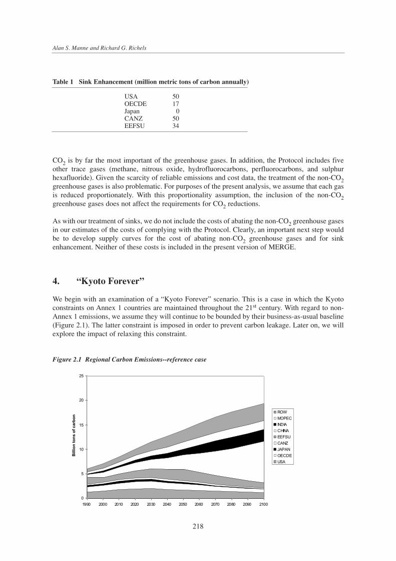
Table 1 Sink Enhancement (million metric tons of carbon annually)
USA 50OECDE 17Japan 0CANZ 50EEFSU 34
CO2 is by far the most important of the greenhouse gases. In addition, the Protocol includes fiveother trace gases (methane, nitrous oxide, hydrofluorocarbons, perfluorocarbons, and sulphurhexafluoride). Given the scarcity of reliable emissions and cost data, the treatment of the non-CO2greenhouse gases is also problematic. For purposes of the present analysis, we assume that each gasis reduced proportionately. With this proportionality assumption, the inclusion of the non-CO2greenhouse gases does not affect the requirements for CO2 reductions.
As with our treatment of sinks, we do not include the costs of abating the non-CO2 greenhouse gasesin our estimates of the costs of complying with the Protocol. Clearly, an important next step wouldbe to develop supply curves for the cost of abating non-CO2 greenhouse gases and for sinkenhancement. Neither of these costs is included in the present version of MERGE.
4. “Kyoto Forever”
We begin with an examination of a “Kyoto Forever” scenario. This is a case in which the Kyotoconstraints on Annex 1 countries are maintained throughout the 21st century. With regard to non-Annex 1 emissions, we assume they will continue to be bounded by their business-as-usual baseline(Figure 2.1). The latter constraint is imposed in order to prevent carbon leakage. Later on, we willexplore the impact of relaxing this constraint.
218
Alan S. Manne and Richard G. Richels
0
5
10
15
20
25
1990 2000 2010 2020 2030 2040 2050 2060 2070 2080 2090 2100
Bill
ion
to
ns
of
carb
on
ROW
MOPEC
INDIA
CHINA
EEFSU
CANZ
JAPAN
OECDE
USA
Figure 2.1 Regional Carbon Emissions--reference case

Numerous studies have shown that global mitigation costs can be reduced substantially by allowingemission reductions to take place wherever it is cheapest to do so - regardless of geographicallocation.The Kyoto Protocol includes several provisions allowing for a limited amount of “where”flexibility. These include emission trading and joint implementation among Annex 1 countries. Theyalso include provisions for a Clean Development Mechanism (CDM) that is intended to facilitatejoint implementation between Annex 1 and non-Annex 1 countries.
As with the definition of sinks, the Protocol leaves many critical details unresolved. For example,it remains unclear whether there will be limits on the extent to which a country can rely upon thepurchase of emission rights to satisfy its obligations. The Protocol states that “the Conference of theParties shall define the relevant principles, modalities, rules and guidelines ...” Similar ambiguitysurrounds the Clean Development Mechanism. Again, the elaboration of “modalities andprocedures” is left to a future meeting of the Conference of the Parties.
In this section, we explore three scenarios: 1) no trading, 2) Annex 1 trading plus CDM, and 3) fullglobal trading. These three options are representative of alternative implementations of the KyotoProtocol. Each has its own advocates and opponents, but we do not consider them equally likely. Inour opinion, there is little likelihood of enticing all major countries to participate in a global marketin emission rights during the initial commitment period (2008-2012). The full global tradingscenario places an upper bound on the CDM’s potential to reduce GDP losses. In calculating thepotential size of the contribution from a CDM, we therefore calculate this upper bound on the exportof emission rights from non-Annex 1 regions. Because of the difficulties in implementation of theCDM, however, we assume that only 15% of the potential would be available for purchase throughthis mechanism. This is a highly subjective estimate. Given the complexities of the CDM, however,we are not inclined to assign a higher value
Figure 4.1 reports the incremental value of carbon emission rights to the US in 2010 and 2020. Wefocus first on 2010. In the most constrained scenario, the US must satisfy its emission reductionrequirements within its own geographical boundaries. In this case, the value of emission rightsapproaches $240 per ton. With Annex 1 trading plus CDM, the value drops to slightly less than $100per ton. As might be expected, the value of emission rights is lowest with full global trading. Here,it falls below $70 per ton.
219
The Kyoto Protocol: A Cost-Effective Strategy for Meeting Environmental Objectives
0
50
100
150
200
250
No Trading Annex1 Trading Plus CDM FullGlobalTrading
$pertonofcarbon
2010
2020
Figure 4.1 Incremental Value of Carbon Emission Rights in US Under Kyoto Forever

For the two scenarios in which trading is permitted, the value of emission rights increases in 2020.This is because EEFSU’s projected emissions lie below its negotiated constraint for 2010. It hasbeen allocated more emission rights than it needs to satisfy its internal obligations. By 2020,however, EEFSU’s economic growth is expected to be such that it no longer enjoys an excess ofemission rights. As a result, there is more competition for emission rights in the internationalmarketplace, and there is an increase in their price.
Another way to view the costs of abatement is to show the GDP losses. Figure 4.2 contains thosefor the US. Losses are highest in the absence of trade. Here, they exceed $80 billion dollars in 2010.This is approximately one percent of US GDP. To the extent that trade is introduced, losses decline.In the most optimistic scenario (full global trade), losses are approximately $20 billion or one-quarter of one percent of GDP in 2010.
Of the three scenarios, “Annex 1 trading plus the CDM” is most consistent with the Protocol as itcurrently stands. However, the US Senate has stated that the US should not be a signatory to theProtocol if it does not mandate specific commitments for developing countries. If this were to resultin full global emission trading, we move in the direction of the right-most bar of Figure 4.2.
There is, however, strong sentiment among many parties to the Framework Convention tosubstantially limit the extent to which Annex 1 countries can meet their obligation through thepurchase of emission rights. Several influential developing countries have expressed strongopposition to the concept altogether. Figure 4.2 shows the costs of the no trading scenario. We nowturn to the case where trading is permitted, but with limitations on the purchase of emission rights.
220
Alan S. Manne and Richard G. Richels
0
20
40
60
80
100
120
No Trading Annex1 Trading Plus CDM FullGlobalTrading
Billionsof1990dollars
2010
2020
Figure 4.2 Annual US GDP Losses Under Kyoto Forever ($billions)
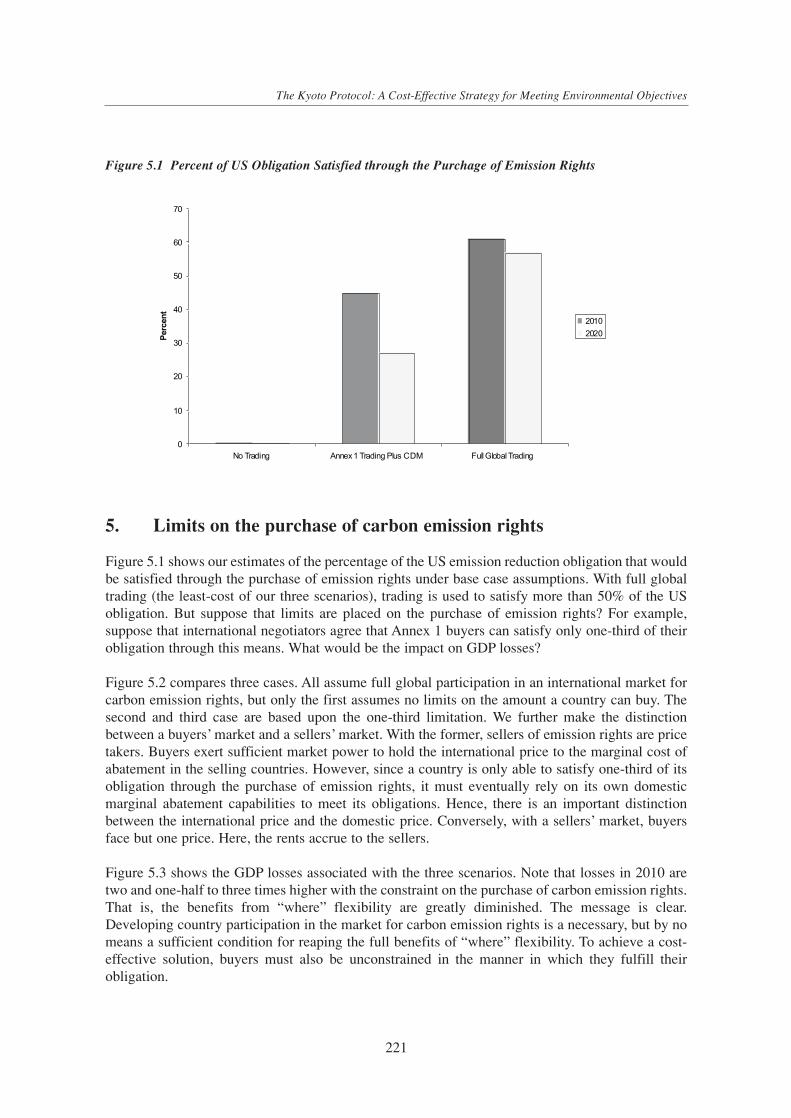
5. Limits on the purchase of carbon emission rights
Figure 5.1 shows our estimates of the percentage of the US emission reduction obligation that wouldbe satisfied through the purchase of emission rights under base case assumptions. With full globaltrading (the least-cost of our three scenarios), trading is used to satisfy more than 50% of the USobligation. But suppose that limits are placed on the purchase of emission rights? For example,suppose that international negotiators agree that Annex 1 buyers can satisfy only one-third of theirobligation through this means. What would be the impact on GDP losses?
Figure 5.2 compares three cases. All assume full global participation in an international market forcarbon emission rights, but only the first assumes no limits on the amount a country can buy. Thesecond and third case are based upon the one-third limitation. We further make the distinctionbetween a buyers’ market and a sellers’ market. With the former, sellers of emission rights are pricetakers. Buyers exert sufficient market power to hold the international price to the marginal cost ofabatement in the selling countries. However, since a country is only able to satisfy one-third of itsobligation through the purchase of emission rights, it must eventually rely on its own domesticmarginal abatement capabilities to meet its obligations. Hence, there is an important distinctionbetween the international price and the domestic price. Conversely, with a sellers’ market, buyersface but one price. Here, the rents accrue to the sellers.
Figure 5.3 shows the GDP losses associated with the three scenarios. Note that losses in 2010 aretwo and one-half to three times higher with the constraint on the purchase of carbon emission rights.That is, the benefits from “where” flexibility are greatly diminished. The message is clear.Developing country participation in the market for carbon emission rights is a necessary, but by nomeans a sufficient condition for reaping the full benefits of “where” flexibility. To achieve a cost-effective solution, buyers must also be unconstrained in the manner in which they fulfill theirobligation.
221
The Kyoto Protocol: A Cost-Effective Strategy for Meeting Environmental Objectives
0
10
20
30
40
50
60
70
No Trading Annex 1 Trading Plus CDM Full Global Trading
Per
cent
2010
2020
Figure 5.1 Percent of US Obligation Satisfied through the Purchage of Emission Rights
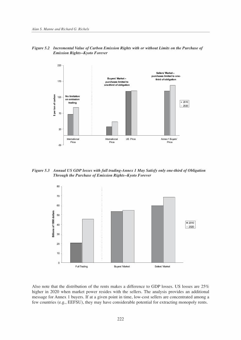
Also note that the distribution of the rents makes a difference to GDP losses. US losses are 25%higher in 2020 when market power resides with the sellers. The analysis provides an additionalmessage for Annex 1 buyers. If at a given point in time, low-cost sellers are concentrated among afew countries (e.g., EEFSU), they may have considerable potential for extracting monopoly rents.
222
Alan S. Manne and Richard G. Richels
-30
20
70
120
170
220
International
Price
International
Price
US Price Annex1 BuyersÕ
Price
$pertonofcarbon
2010
2020
BuyersÕ Market --
purchases limited to
one-third of obligation
SellersÕMarket --
purchases limited to one-
third ofobligation
No limitation
on emission
trading
0
10
20
30
40
50
60
70
80
Full Trading BuyersÕMarket SellersÕMarket
Billionsof1990dollars
2010
2020
Figure 5.2 Incremental Value of Carbon Emission Rights with or without Limits on the Purchase of Emission Rights--Kyoto Forever
Figure 5.3 Annual US GDP losses with full trading-Annex 1 May Satisfy only one-third of Obligation Through the Purchase of Emission Rights--Kyoto Forever
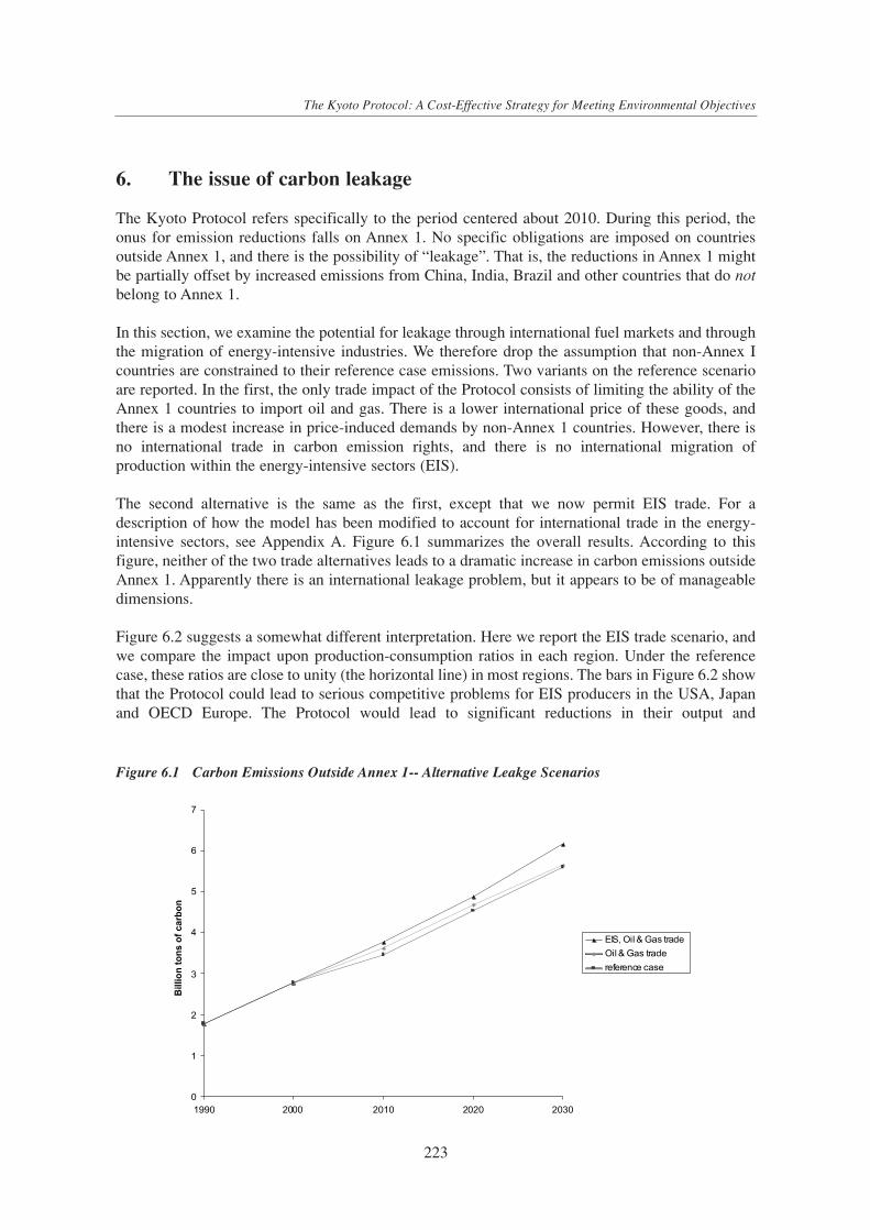
6. The issue of carbon leakage
The Kyoto Protocol refers specifically to the period centered about 2010. During this period, theonus for emission reductions falls on Annex 1. No specific obligations are imposed on countriesoutside Annex 1, and there is the possibility of “leakage”. That is, the reductions in Annex 1 mightbe partially offset by increased emissions from China, India, Brazil and other countries that do notbelong to Annex 1.
In this section, we examine the potential for leakage through international fuel markets and throughthe migration of energy-intensive industries. We therefore drop the assumption that non-Annex Icountries are constrained to their reference case emissions. Two variants on the reference scenarioare reported. In the first, the only trade impact of the Protocol consists of limiting the ability of theAnnex 1 countries to import oil and gas. There is a lower international price of these goods, andthere is a modest increase in price-induced demands by non-Annex 1 countries. However, there isno international trade in carbon emission rights, and there is no international migration ofproduction within the energy-intensive sectors (EIS).
The second alternative is the same as the first, except that we now permit EIS trade. For adescription of how the model has been modified to account for international trade in the energy-intensive sectors, see Appendix A. Figure 6.1 summarizes the overall results. According to thisfigure, neither of the two trade alternatives leads to a dramatic increase in carbon emissions outsideAnnex 1. Apparently there is an international leakage problem, but it appears to be of manageabledimensions.
Figure 6.2 suggests a somewhat different interpretation. Here we report the EIS trade scenario, andwe compare the impact upon production-consumption ratios in each region. Under the referencecase, these ratios are close to unity (the horizontal line) in most regions. The bars in Figure 6.2 showthat the Protocol could lead to serious competitive problems for EIS producers in the USA, Japanand OECD Europe. The Protocol would lead to significant reductions in their output and
223
The Kyoto Protocol: A Cost-Effective Strategy for Meeting Environmental Objectives
0
1
2
3
4
5
6
7
1990 2000 2010 2020 2030
Billiontonsofcarbon
EIS, Oil & Gas trade
Oil & Gas trade
reference case
Figure 6.1 Carbon Emissions Outside Annex 1-- Alternative Leakge Scenarios
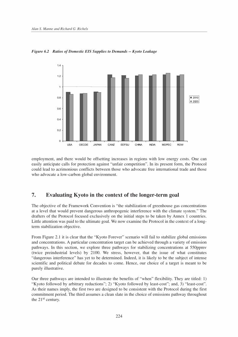
employment, and there would be offsetting increases in regions with low energy costs. One caneasily anticipate calls for protection against “unfair competition”. In its present form, the Protocolcould lead to acrimonious conflicts between those who advocate free international trade and thosewho advocate a low-carbon global environment.
7. Evaluating Kyoto in the context of the longer-term goal
The objective of the Framework Convention is “the stabilization of greenhouse gas concentrationsat a level that would prevent dangerous anthropogenic interference with the climate system.” Thedrafters of the Protocol focused exclusively on the initial steps to be taken by Annex 1 countries.Little attention was paid to the ultimate goal. We now examine the Protocol in the context of a long-term stabilization objective.
From Figure 2.1 it is clear that the “Kyoto Forever” scenario will fail to stabilize global emissionsand concentrations. A particular concentration target can be achieved through a variety of emissionpathways. In this section, we explore three pathways for stabilizing concentrations at 550ppmv(twice preindustrial levels) by 2100. We stress, however, that the issue of what constitutes“dangerous interference” has yet to be determined. Indeed, it is likely to be the subject of intensescientific and political debate for decades to come. Hence, our choice of a target is meant to bepurely illustrative.
Our three pathways are intended to illustrate the benefits of “when” flexibility. They are titled: 1)“Kyoto followed by arbitrary reductions”; 2) “Kyoto followed by least-cost”; and, 3) “least-cost”.As their names imply, the first two are designed to be consistent with the Protocol during the firstcommitment period. The third assumes a clean slate in the choice of emissions pathway throughoutthe 21st century.
224
Alan S. Manne and Richard G. Richels
0
0.2
0.4
0.6
0.8
1
1.2
1.4
USA OECDE JAPAN CANZ EEFSU CHINA INDIA MOPEC ROW
2010
2020
Figure 6.2 Ratios of Domestic EIS Supplies to Demands -- Kyoto Leakage

For the first scenario, we assume that Annex 1 countries reduce emissions through 2030 at the samerate as the OECD during the first decade of the 21st century (2% per year). During this period, nonAnnex-1 countries are permitted to emit up to their reference case levels. By 2020, emissions in thedeveloping nations are larger than those in Annex I. We then choose a pathway to stabilizationwhich represents a relatively smooth transition to the target. As for the post-2030 burden-sharingscheme, we assume that between 2030 and 2050 all regions move to equal per capita emission rights(based on their 1990 population). Equal per capita emission rights have been proposed as oneapproach to international fairness, but there are others that might also serve to separate the issue ofequity from that of economic efficiency.
With “Kyoto followed by least-cost”, the Protocol is adopted for the initial commitment period.Thereafter, the most cost-effective pathway is followed for stabilizing concentrations at 550ppmv.With “least-cost”, the most cost-effective pathway for stabilizing concentrations at 550ppmv isfollowed from the outset. The latter two scenarios adopt the same proportionate burden-sharingscheme as the first.
All three scenarios assume Annex 1 trading plus the CDM. However, they differ as to the timing ofdeveloping country involvement in the international market for carbon emission rights. Bydefinition, least-cost assumes that emission reductions will be made where it is cheapest to do so,regardless of the geographical location. Hence, in the least-cost scenario, we assume globalemission trading from the outset. In the case of “Kyoto followed by least-cost”, we assume thatglobal emission trading is delayed until after the first commitment period. With “Kyoto followed byarbitrary reductions”, global emission trading does not begin until 2030, the year that developingcountries agree to lower their emissions below business-as-usual.
Global carbon emissions. Figure 7.1 shows global carbon emissions for the reference case and thethree stabilization scenarios. Following a least-cost strategy from the outset results in an emissionspathway that tracks the reference path through 2010 and then departs at an increasing rate thereafter.
225
The Kyoto Protocol: A Cost-Effective Strategy for Meeting Environmental Objectives
0
5
10
15
20
25
2000 2010 2020 2030 2040 2050 2060 2070 2080 2090 2100
Billiontonsofcarbon
reference least-cost Kyoto followedby least-cost Kyoto followed byarbitrary reductions
Figure 7.1 Global Carbon Emissions - Reference case and three alternative emission pathways for stabilizing Concentrations at 550 ppmv
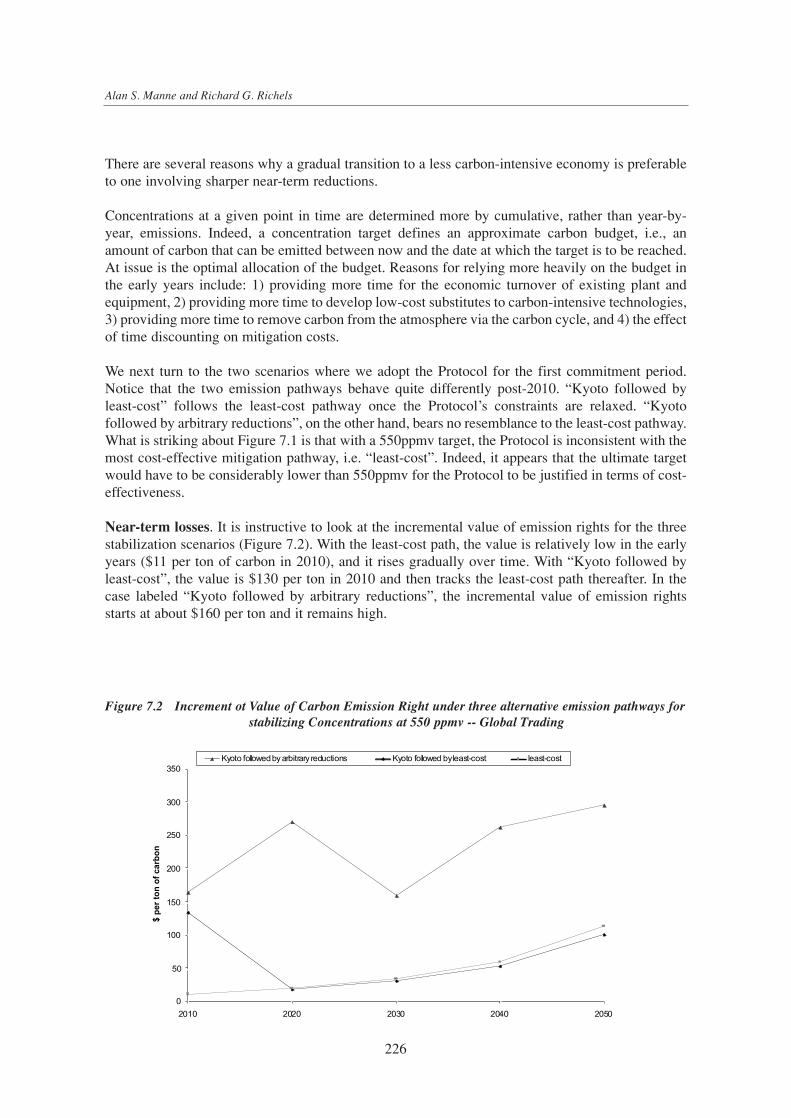
There are several reasons why a gradual transition to a less carbon-intensive economy is preferableto one involving sharper near-term reductions.
Concentrations at a given point in time are determined more by cumulative, rather than year-by-year, emissions. Indeed, a concentration target defines an approximate carbon budget, i.e., anamount of carbon that can be emitted between now and the date at which the target is to be reached.At issue is the optimal allocation of the budget. Reasons for relying more heavily on the budget inthe early years include: 1) providing more time for the economic turnover of existing plant andequipment, 2) providing more time to develop low-cost substitutes to carbon-intensive technologies,3) providing more time to remove carbon from the atmosphere via the carbon cycle, and 4) the effectof time discounting on mitigation costs.
We next turn to the two scenarios where we adopt the Protocol for the first commitment period.Notice that the two emission pathways behave quite differently post-2010. “Kyoto followed byleast-cost” follows the least-cost pathway once the Protocol’s constraints are relaxed. “Kyotofollowed by arbitrary reductions”, on the other hand, bears no resemblance to the least-cost pathway.What is striking about Figure 7.1 is that with a 550ppmv target, the Protocol is inconsistent with themost cost-effective mitigation pathway, i.e. “least-cost”. Indeed, it appears that the ultimate targetwould have to be considerably lower than 550ppmv for the Protocol to be justified in terms of cost-effectiveness.
Near-term losses. It is instructive to look at the incremental value of emission rights for the threestabilization scenarios (Figure 7.2). With the least-cost path, the value is relatively low in the earlyyears ($11 per ton of carbon in 2010), and it rises gradually over time. With “Kyoto followed byleast-cost”, the value is $130 per ton in 2010 and then tracks the least-cost path thereafter. In thecase labeled “Kyoto followed by arbitrary reductions”, the incremental value of emission rightsstarts at about $160 per ton and it remains high.
226
Alan S. Manne and Richard G. Richels
0
50
100
150
200
250
300
350
2010 2020 2030 2040 2050
$pertonofcarbon
Kyoto followedbyarbitrary reductions Kyoto followed byleast-cost least-cost
Figure 7.2 Increment ot Value of Carbon Emission Right under three alternative emission pathways forstabilizing Concentrations at 550 ppmv -- Global Trading

Figure 7.3 shows US GDP losses in 2010 and 2020 under the three stabilization scenarios. Noticethat GDP losses in 2010 differ for the two scenarios involving the initial adoption of the Protocol.Because of the long-lived nature of energy investments, investors are concerned both with whathappens in the initial commitment period and what happens thereafter. In the case of the more rapidtransition away from the baseline (“Kyoto followed by arbitrary reductions”), investors will beforced to invest more heavily in high–cost substitutes in the early years. With “Kyoto followed byleast-cost”, they will have more flexibility.
It is striking by how much GDP losses can be lowered under the “least-cost” scenario. This strategyinvolves a more gradual transition away from the baseline in the early years. It relieves much of thepressure for premature retirement of existing plant and equipment and for dependence on high-costsubstitutes (both on the supply- and demand-sides of the energy sector). Relative to the referencecase, the US also receives some benefits as an oil importer. Recall that a carbon constraint decreasesthe overall demand for oil and lowers its price on the international market.
Global losses. Finally, it is instructive to examine losses from a global perspective (Figure 7.4). Forpurposes of the present comparison, we focus on the present value of consumption losses over the21st century discounted to 1990 at 5 percent. The relative magnitude of the cumulative losses for thethree stabilization scenarios comes as no surprise given the previous discussion. “Kyoto followedby arbitrary reductions” is by far the most expensive of the three paths. “Kyoto followed by least-cost” is a considerable improvement, but is still 40% more expensive than embarking on the most cost-effective mitigationpathway from the outset.
What is surprising is that “Kyoto Forever” turns out to be more expensive than “Kyoto followed byleast cost” or “least cost”. “Kyoto Forever” results in sharper global emission reductions during theearly decades of the 21st century. It does not, however, succeed in stabilizing emissions, much lessconcentrations. By contrast, the other scenarios all lead to stabilization at 550ppmv. In other words,“Kyoto Forever” ends up costing more, and it buys less long-term protection.
227
The Kyoto Protocol: A Cost-Effective Strategy for Meeting Environmental Objectives
0
20
40
60
80
100
120
140
Kyoto followedbyarbitrary
reductions
Kyoto folowed byll east-cost least-cost
Billionsof1990dollars
2010
2020
Figure 7.3 US GDP Losses under three alternative 550 ppmvStabilization Scenarios

8. Further comments
Some suggest that models such as MERGE tend to overestimate the costs of mitigation. They arguethat, when prospects for technical progress are incorporated, the costs of a carbon constraint, evena sharp near-term constraint, will be minimal. We, too, are optimistic about the outlook for technicalinnovation. Indeed, such innovation is embedded both in our reference case and in the policyscenarios. The disagreement is over the rate at which such progress will occur. We do not believethat economically competitive substitutes will become available at such a rate as to trivialize thecosts of a Kyoto-like Protocol.
A more valid concern may be that we are underestimating the costs of a carbon constraint. There areseveral reasons why this may be the case. To begin with, optimization models assume that decisionmakers have perfect foresight. That is, they assume that investors are fully informed about thenature of future constraints, and act accordingly. Given the present state of uncertainty, this is highlyunlikely. Models such as MERGE also tend to ignore short-term macro shocks. For example, thehigher energy prices brought about by a carbon constraint are likely to be inflationary. If this leadsto higher interest rates, investment may be dampened. The result would be a slowdown in economicgrowth.
In addition, we assume that policies will be efficient. That is, market mechanisms will be chosenover “command and control” approaches to accomplishing environmental objectives. Whereas, inrecent years, there has been an increasing trend toward market mechanisms, the approach to betaken with climate policy is by no means assured. Moreover, even if such a commitment were made,we have no assurances that the requisite international institutions will be available when needed.
Although it is easy to quibble over the numbers, the real value of analyses lies more in insights thanin numerical values. And, indeed we believe that the current exercise has yielded several insights
228
Alan S. Manne and Richard G. Richels
0
500
1000
1500
2000
2500
Kyoto forever Kyoto followed by arbitrary reductions
Kyoto followed by least-cost
least-cost
Bill
ions
of 1
990
dolla
rsFigure 7.4 Global Consumption Losses through 2100 discounted to 1990 at 5% -- Kyoto Forever vs.
Three Scenarios for Stabilizing Concentrations at 550 ppmv

that may be of value to those charged with interpreting the current proposal. Here, we summarizewhat we have learned:
• First, it is extremely unlikely that a “Kyoto Forever” scenario will stabilize emissions — muchless concentrations. Non-Annex 1 emissions are quickly overtaking those of the OECD and theeconomies in transition. Hence, meeting the stabilization goal of the Framework Convention willeventually require the participation of developing countries.
• International cooperation through trade in emission rights is essential if we are to reducemitigation costs. The magnitude of the savings will depend on several factors. These include thenumber of countries participating in the trading market, the shape of each country’s marginalabatement cost curve, and the extent to which buyers can satisfy their obligation through thepurchase of emission rights.
• With regard to the latter, limitations on the purchase of emission rights may be especially costly.In the example explored here, limiting purchases to one-third of a country’s obligation increasedGDP losses by a factor of at least two and one-half in the year 2010. If proponents of suchlimitations are successful, they may seriously reduce the benefits from “where” flexibility.
• The issue of monopoly power in markets for emission rights may turn out to be important. Thisis most likely to occur if trading is limited to Annex 1 and the majority of inexpensive emissionrights are concentrated in a small number of countries. If these countries were successful inorganizing a sellers’ cartel, they might be able to extract sizable rents.
• The near-term costs of the Protocol will depend on expectations regarding the future. Energyinvestments are typically long-lived. Today’s investment decisions are not only influenced bywhat happens during the next decade, but also by what happens thereafter. Hence, analyseswhich focus solely on 2010 may be underestimating the costs of Kyoto.
• Finally, and perhaps most importantly, unless the concentration target for CO2 is well below550ppmv, the Protocol appears to be inconsistent with a cost-effective long-term strategy forstabilizing CO2 concentrations. Rather than requiring sharp near-term reductions, it appears thata more sensible strategy would be to make the transition at the point of capital stock turnover.This would eliminate the need for premature retirement of existing plant and equipment andwould provide the time that is needed to develop low-cost, low-carbon substitutes.
229
The Kyoto Protocol: A Cost-Effective Strategy for Meeting Environmental Objectives

Appendix A. Modeling international trade in the energy-intensive sectors
MERGE 3.0 has recently been modified to include the possibility of trade in EIS (energy-intensivesectors). EIS is an aggregate including ferrous and non-ferrous metals, chemicals, nonmetallicminerals, paper, pulp and print. This aggregate does not include the energy-intensive industry ofpetroleum refining. The model may be run either with or without EIS trade.
The new feature is introduced in a way that preserves the basic simplifying characteristics of theETA-MACRO submodel. That is, energy, capital and labor are substitutes that enter into anaggregate production function. They produce a numeraire good which may be used forconsumption, investment and interindustry payments for energy costs.
It is assumed that trade will continue to represent a relatively small amount of each region’s totalinternal demand for EIS. The GTAP (General Trade Analysis Program, 1992) data base is employedto estimate each region’s EIS demands. In all other respects, the model is the same as MERGE 3.0.
For projecting the impact of the Kyoto protocol, each region is taken to be self-sufficient at baseyear energy prices. Changes in the location of production are attributed primarily to changes in thecost of energy. At base year prices in the USA, 85% of the cost of EIS consisted of non-energyinputs (labor, shipping, capital, iron ore, etc.), and 15% of the cost consisted of energy inputs (halfelectric and half non-electric). Under these conditions, a doubling of energy prices would implyonly a 15% increase in the cost of EIS. This is why it is assumed that the demand for EIS is inelasticwith respect to the price of energy. For projecting future demands, the income elasticity is taken tobe 0.5.
230
Alan S. Manne and Richard G. Richels
Figure A.1 EIS Supply Curves -- Marginal Cost of Non-Energy Inputs to EIS
0
0.5
1
1.5
0 0.5 1 1.5
Fraction of region's demand supplied domestically
Fra
ctio
n o
f ave
rag
e co
st c
oef
fici
ent i
n U
SA
Heckscher-Ohlinfractions:
0.5
1.0
Figure A.1 EIS Supply Curves -- Marginal Cost of Non-Energy Inputs to EIS
For modeling purposes, we have supposed that the marginal supplies of EIS in all regions aredetermined by the same international technology that prevails in the USA. Each region has the sameenergy-EIS production ratio. For non-energy inputs, each supply curve is linear. Its positive slopeserves the same purpose as an Armington elasticity describing substitution between foreign anddomestic goods. This is the way in which we avoid penny-switching as a characteristic solutionmode.
The slope of the non-energy supply curve is described as a Heckscher-Ohlin fraction. If this fractionis unity, EIS is viewed as a perfectly homogeneous commodity. Small changes in energy costs willthen lead to large changes in the international location of production. If this fraction is less thanunity, the supply function is less elastic, and the changes in location will be less dramatic. (SeeFigure A.1.)
231
The Kyoto Protocol: A Cost-Effective Strategy for Meeting Environmental Objectives
References
Conference of the Parties (1997). “Kyoto Protocol to theUnited Nations Framework Convention on ClimateChange”, Third Session Kyoto, 1-10 December.Intergovernmental Negotiating Committee for AFramework Convention on Climate Change (1992).Fifth Session, Second Part, New York, 30 April-9 May.IPCC (1994). Climate Change 1994, CambridgeUniversity Press.
IPCC (1997). “Stabilization of Atmospheric GreenhouseGases: Physical, Biological and Socio-EconomicImplications”, Technical Paper III.
Manne, A., Mendelsohn, R., and Richels, R. (1995).“MERGE: a model for evaluating regional and globaleffects of GHG reduction policies”, Energy Policy, 3 (1).
Manne, A., and Richels, R. (1995). “The GreenhouseDebate: economic efficiency, burden sharing andhedging strategies”, The Energy Journal, 16 (4).Richels, R., Edmonds, J., Gruenspecht, H., and Wigley,T. (1996). “The Berlin Mandate: The Design of CostEffective Mitigation Strategies”, EMF-14, WorkingPaper 3, Stanford University, Stanford, CA.
US Congress (1997). 105th Congress, 1st Session (1997), S.Res. 98.
Wigley, T., Richels, R., and Edmonds, J. (1996).“Economic and Environmental Choices in theStabilization of Atmospheric CO2 Concentrations”,Nature, Vol. 379, 18 January.

232

Discussion
ZhongXiang Zhang1
1. Introduction
Prof. Manne and Dr. Richels have made many valuable contributions in modelling the economiccosts of mitigating greenhouse gas emissions, and this paper (Manne and Richels, 1999) is one ofthese contributions. It first examines a “Kyoto Forever” scenario in which the Kyoto constraints onAnnex I countries are maintained throughout the 21st century. Next, the paper calculates what theeconomic implications of limiting the purchase of carbon emission rights are. It shows that in caseAnnex I buyers are allowed to meet only one-third of their obligation through trading of carbonrights, the annual GDP losses in 2010 in the US are two and one-half to three times the case in whichfull global trading is assumed. Then, the paper examines the potential of carbon leakage throughinternational fuel markets and through the migration of energy-intensive industries from Annex Icountries to non-Annex I countries. Finally, the paper evaluates the Kyoto Protocol in the contextof the longer-term goal of the Framework Convention.
Reading this very interesting paper suggests four issues or questions to me. The first issue is aboutdistributional realities of the international climate change negotiations. The second issue is aboutcorrespondence between geopolitical regional aggregates in MERGE and Annex B countries. Thethird issue is about implications of the autonomous energy efficiency improvement rates assumedin MERGE on the income elasticity of energy consumption. And fourth issue is about market powerin an international greenhouse gas emissions trading scheme.
2. Modelling distributional realities of the international climate change negotiations
First of all, I agree with the broad conclusion of the paper (Manne and Richels, 1999) that a long-term climate strategy should be designed to facilitate achieving the Framework Convention’sultimate objective of stabilizing greenhouse gas concentrations in the atmosphere at the lowestpossible abatement and transaction costs. One might wonder why keeping down the costs ofcompliance matters. It is often heard that the high cost of compliance is just what polluters shouldsuffer so that polluters are taught a lesson. From a political perspective, the more costly thecompliance, the less likely it is that those who bear the high costs will be willing to commit tostringent emissions targets in the future. Given the fact that no emissions targets beyond 2012 havebeen set, increasing the overall costs of compliance thus makes it even more difficult to set stringentemissions targets for some Annex B countries, if not all, for the subsequent commitment periods
233
The Kyoto Protocol: A Cost-Effective Strategy for Meeting Environmental Objectives
1 The views expressed here are those of the author. The author bears sole responsibility for any errors and omissions that may remain.

beyond 2012 in order to achieve the Climate Convention’s ultimate objective.2 It is the lack of thetargets of post-2012 that is seen as a threat to the pace of technical innovation needed to make morestringent future emissions targets affordable. The lack of such long-term commitments also restrictsthe choice of the compliance mechanisms and tools and creates some divergence of views inassigning liability in an international greenhouse gas emissions trading scheme (Zhang, 1999).
There are many paths to a longer-term stabilization concentration target. The path of offering greatwhen flexibility, namely, the path that would begin gradually and leave the more drastic cuts inemissions in later periods, receives increased attention in the literature on economic andenvironmental implications of reaching a specific atmospheric concentration target (see, forexample, Richels and Edmonds, 1995; Wigley, Richels and Edmonds, 1996; Manne and Richels,1998; Yang and Jacoby, 1999). However, as Jacoby et al. point out, although these studies areinstructive, their emphasis on global cost-effectiveness tends to underplay important distributionalrealities of the international climate change negotiations, and how they might be worked out overtime. With the successful conclusion of the Montreal Protocol that sets percentage reduction targetsfor CFC emissions, it is not surprising that calls for limiting greenhouse gas emissions have focusedon a similar strategy since the June 1988 Toronto Conference, which has recommended a 20%reduction by 2005 and a 50% reduction by 2025 in global CO2 emissions relative to the 1988 levels(Zhang, 1997). Although it is the accumulated concentration of greenhouse gases in the atmosphere,not the annual emissions, that influences climate change, as at Kyoto, negotiations will continue tobe about emissions levels in the near term, not about emission trajectories over several decades. Inmy review, the main reason is that, in the absence of dramatic and forceful changes from thebusiness-as-usual trends, negotiators, particularly from developing countries, believe that privatefirms and consumers alike will not change their production and consumption patterns and will nottake seriously the need to reduce greenhouse gas emissions.3 The question then arises: how can oneconnect negotiations about near-term emissions reductions with a long-term stabilization objective?With the belief that in any fair regime substantial differences in per capita income will translate intosubstantial differences in emissions control obligations, Jacoby et al. (1999), for example, proposethat accession of developing countries and burden sharing should be based on ability of pay.Although it is not my intention to recommend the approach as the sole determinant of incrementalemissions control obligations, it might be worthwhile pursuing this kind of thought in assumingnational commitments in MERGE towards the lowest cost path to the longer-term stabilizationconcentration target. This would enrich the policy relevance of this study to the ongoing climatechange negotiations.
3. Correspondence between geopolitical regional aggregates in MERGE and Annex B countries
It is unclear whether the correspondence between geopolitical regional aggregates in MERGE andAnnex B countries is exact. It seems to me that Annex B countries modelled in MERGE constituteall the OECD countries and Eastern Europe and the Former Soviet Union (EEFSU). As such, they
234
ZhongXiang Zhang
2 Stavins (1998) points out that the adoption of the US SO2 allowance trading program is largely attributed to strong support from theEnvironmental Defense Fund that was able to make powerful arguments for tradeable permits on the grounds that the use of a cost-effective instrument would make it politically feasible to achieve greater reductions in SO2 emissions than would otherwise be possible.I believe that the arguments also hold for setting the post-2012 greenhouse gas emissions targets.
3 Negotiating the appropriate size and shape of percentage emissions reductions would be not that easy. On the one hand, whatever atarget is agreed on should be large enough to signal a decisive change from the business-as-usual trends. On the other hand, it should notbe so large that governments would dismiss it as unrealistic.
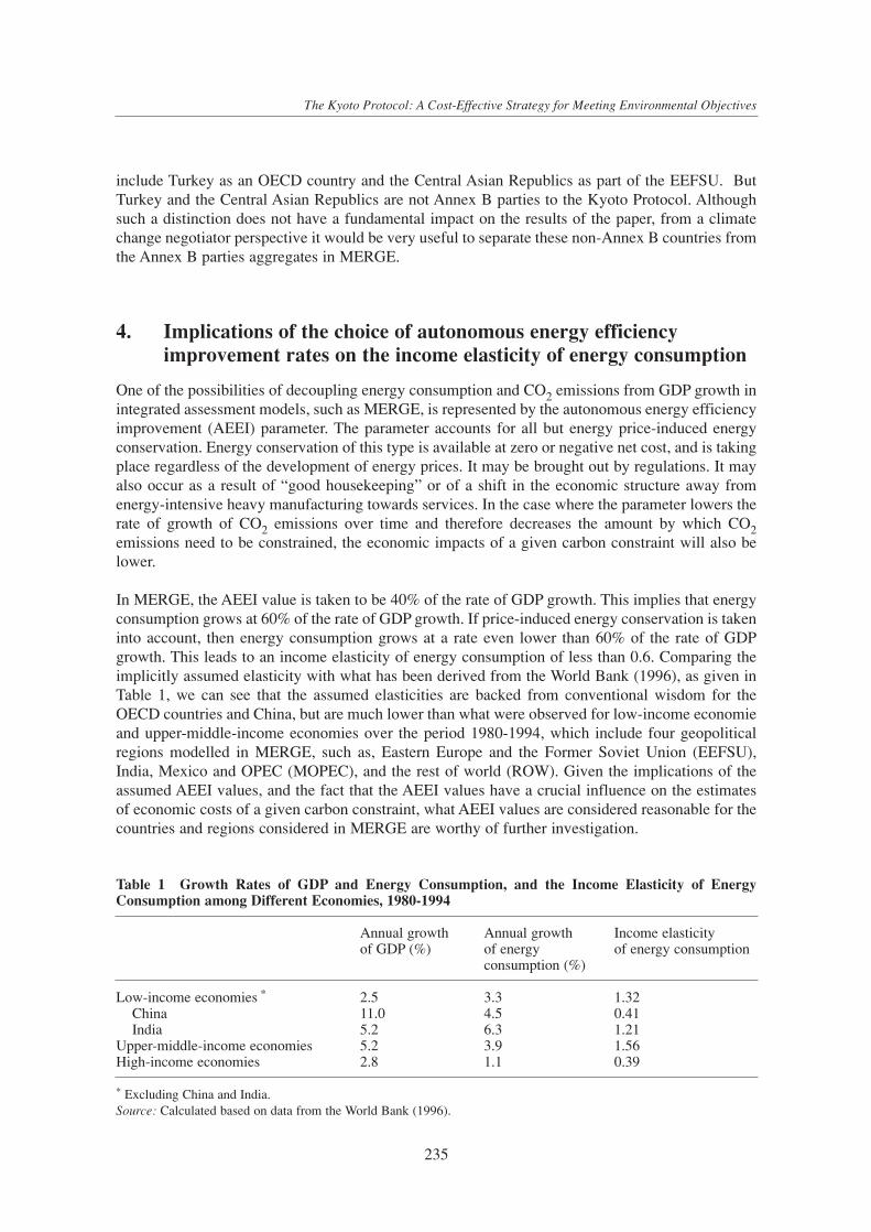
include Turkey as an OECD country and the Central Asian Republics as part of the EEFSU. ButTurkey and the Central Asian Republics are not Annex B parties to the Kyoto Protocol. Althoughsuch a distinction does not have a fundamental impact on the results of the paper, from a climatechange negotiator perspective it would be very useful to separate these non-Annex B countries fromthe Annex B parties aggregates in MERGE.
4. Implications of the choice of autonomous energy efficiencyimprovement rates on the income elasticity of energy consumption
One of the possibilities of decoupling energy consumption and CO2 emissions from GDP growth inintegrated assessment models, such as MERGE, is represented by the autonomous energy efficiencyimprovement (AEEI) parameter. The parameter accounts for all but energy price-induced energyconservation. Energy conservation of this type is available at zero or negative net cost, and is takingplace regardless of the development of energy prices. It may be brought out by regulations. It mayalso occur as a result of “good housekeeping” or of a shift in the economic structure away fromenergy-intensive heavy manufacturing towards services. In the case where the parameter lowers therate of growth of CO2 emissions over time and therefore decreases the amount by which CO2emissions need to be constrained, the economic impacts of a given carbon constraint will also belower.
In MERGE, the AEEI value is taken to be 40% of the rate of GDP growth. This implies that energyconsumption grows at 60% of the rate of GDP growth. If price-induced energy conservation is takeninto account, then energy consumption grows at a rate even lower than 60% of the rate of GDPgrowth. This leads to an income elasticity of energy consumption of less than 0.6. Comparing theimplicitly assumed elasticity with what has been derived from the World Bank (1996), as given inTable 1, we can see that the assumed elasticities are backed from conventional wisdom for theOECD countries and China, but are much lower than what were observed for low-income economieand upper-middle-income economies over the period 1980-1994, which include four geopoliticalregions modelled in MERGE, such as, Eastern Europe and the Former Soviet Union (EEFSU),India, Mexico and OPEC (MOPEC), and the rest of world (ROW). Given the implications of theassumed AEEI values, and the fact that the AEEI values have a crucial influence on the estimatesof economic costs of a given carbon constraint, what AEEI values are considered reasonable for thecountries and regions considered in MERGE are worthy of further investigation.
235
The Kyoto Protocol: A Cost-Effective Strategy for Meeting Environmental Objectives
Table 1 Growth Rates of GDP and Energy Consumption, and the Income Elasticity of EnergyConsumption among Different Economies, 1980-1994
Annual growth Annual growth Income elasticity of GDP (%) of energy of energy consumption
consumption (%)
Low-income economies * 2.5 3.3 1.32China 11.0 4.5 0.41India 5.2 6.3 1.21
Upper-middle-income economies 5.2 3.9 1.56High-income economies 2.8 1.1 0.39
* Excluding China and India.Source: Calculated based on data from the World Bank (1996).
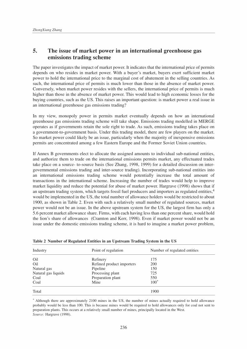
5. The issue of market power in an international greenhouse gas emissions trading scheme
The paper investigates the impact of market power. It indicates that the international price of permitsdepends on who resides in market power. With a buyer’s market, buyers exert sufficient marketpower to hold the international price to the marginal cost of abatement in the selling countries. Assuch, the international price of permits is much lower than those in the absence of market power.Conversely, when market power resides with the sellers, the international price of permits is muchhigher than those in the absence of market power. This would lead to high economic losses for thebuying countries, such as the US. This raises an important question: is market power a real issue inan international greenhouse gas emissions trading?
In my view, monopoly power in permits market eventually depends on how an internationalgreenhouse gas emissions trading scheme will take shape. Emissions trading modelled in MERGEoperates as if governments retain the sole right to trade. As such, emissions trading takes place ona government-to-government basis. Under this trading model, there are few players on the market.So market power could likely be an issue, particularly when the majority of inexpensive emissionspermits are concentrated among a few Eastern Europe and the Former Soviet Union countries.
If Annex B governments elect to allocate the assigned amounts to individual sub-national entities,and authorize them to trade on the international emissions permits market, any effectuated tradestake place on a source- to-source basis (See Zhang, 1998, 1999) for a detailed discussion on inter-governmental emissions trading and inter-source trading). Incorporating sub-national entities intoan international emissions trading scheme would potentially increase the total amount oftransactions in the international scheme. Increasing the number of trades would help to improvemarket liquidity and reduce the potential for abuse of market power. Hargrave (1998) shows that ifan upstream trading system, which targets fossil fuel producers and importers as regulated entities,4
would be implemented in the US, the total number of allowance holders would be restricted to about1900, as shown in Table 2. Even with such a relatively small number of regulated sources, marketpower would not be an issue. In the above upstream system for the US, the largest firm has only a5.6 percent market allowance share. Firms, with each having less than one percent share, would holdthe lion’s share of allowances (Cramton and Kerr, 1998). Even if market power would not be anissue under the domestic emissions trading scheme, it is hard to imagine a market power problem,
236
ZhongXiang Zhang
Table 2 Number of Regulated Entities in an Upstream Trading System in the US
Industry Point of regulation Number of regulated entities
Oil Refinery 175Oil Refined product importers 200Natural gas Pipeline 150Natural gas liquids Processing plant 725Coal Preparation plant 550Coal Mine 100*
Total 1900
* Although there are approximately 2100 mines in the US, the number of mines actually required to hold allowanceprobably would be less than 100. This is because mines would be required to hold allowances only for coal not sent topreparation plants. This occurs at a relatively small number of mines, principally located in the West.Source: Hargrave (1998).

if trading is broadened beyond the national boundary and provided that requisite internationalinstitutions supporting trading are available. So, in my review, the results as estimated by MERGEunder the assumption of market power should be regarded as an upper bound on the price of carbonpermits and the GDP losses.
However, collusive behaviour might occur under the CDM, because both host and investorgovernments do play the role in approving CDM projects, whereas, under inter-source trading, thegovernments are limited to setting the rules rather than undertaking emissions trading themselves.This raises the question that how developing countries can limit the supply of CDM credits andmaximize the revenues of selling CDM credits. Figure 1 shows an aggregated downward-slopingdemand curve of Annex I countries and an aggregated upward-sloping supply curve of non-AnnexI countries to supply the total quantity of CDM credits at various price levels (for simplicity, I drawlinear demand and supply curves here). The point Eo where the two curves labelled as Demand andSupplyo cross gives the market cleaning price of CDM credits Po and the total quantity of CDMcredits traded Qo. The area OEoPo represents the net gain to non-Annex I countries. Then, how toincrease the net gain to non-Annex I countries? As shown in Figure 1, this could be achieved byshifting supply curve upward from Supplyo to Supply*. At the new equilibrium E* where the newsupply curve Supply* crosses the same demand curve Demand, although the total quantity of CDM
237
The Kyoto Protocol: A Cost-Effective Strategy for Meeting Environmental Objectives
4 In contrast, a downstream trading system would be applied at the point of emissions. As such, a large number of diverse energy usersare included. See Zhang (1998, 1999) for a detailed discussion on upstream, downstream and hybrid emissions trading systems.
5 When emissions trading were allowed, a country whose legally binding greenhouse gas emissions limits set by the Kyoto Protocolexceed its actual or anticipated emissions requirements would be able to trade these excess emissions, thus creating the hot air that wouldotherwise have not occurred. The hot air problem would be particularly acute in Russia whose emissions are not expected to rise to its1990 level until 2010 (UNFCCC, 1997).
Demand
Supply*
Supplyo
E*
Eo
P*
Po
O Q* Qo
Quantity of CDM credits
Pric
e of
CD
M c
redi
ts
Figure 1 Aggregated Demand and Supply Curves of CDM Credits
credits traded drops to Q*, the net gain OE*P* is greater than OEoPo because the market clearingprice P* rises faster than the quantity falls. This has a very important policy implication, as itsuggests that if the market clearing price could be held up to the reasonable level, relatively costlyCDM projects could be undertaken early with international partners. This would leave low-costabatement options (the so-called low-hanging fruits) available for later use of their own ifdeveloping countries would be subsequently required to reduce their own emissions.
The question then arises: how can the market price of CDM credits could be raised? One tacitcollusive strategy is that developing countries could insist on restriction on the use of flexibilitymechanisms to meet Annex I countries’ Kyoto commitments in the name of promoting technicalinnovation needed to make more stringent future emissions targets affordable and thus kick off theball to Annex I countries’ court. Another way is to prevent trading in hot air, although in practice itis very difficult to distinguish real reduction from hot air.5 Because hot air is available at zeroabatement cost, allowing hot air to be traded tends to push down the overall market clearing pricebecause it reduces Annex I countries’ demand for CDM credits. It has dawned on many developingcountries and environmental NGOs that the US is counting on breathing Russian hot air to complywith its reduction target set in the Kyoto Protocol, rather than taking abatement actions at home. Inthis regard, it would be very helpful to clear up the doubt about this, if MERGE could provide theestimated amount of hot air and estimate the economic implications of excluding trading in hot airon the US economy.
238
ZhongXiang Zhang
References
Cramton, P. and S. Kerr (1998), Tradeable CarbonAllowance Auctions: How and Why to Auction,University of Maryland at College Park.
Hargrave, T. (1998), US Carbon Emissions Trading:Description of an Upstream Approach, Center for ClearAir Policy, Washington, DC.
Jacoby, H.D., Schmalensee, R. and I.S. Wing (1999),Toward a Useful Architecture for Climate ChangeNegotiations, MIT Joint Program on the Science andPolicy of Global Change, Report No. 49, MassachusettsInstitute of Technology.
Manne, A. and R. Richels (1997), On Stabilizing CO2Concentrations: Cost-Effective Emission ReductionStrategies, Environmental Modeling and Assessment,Vol. 2, No. 4, pp. 251-265.
Manne, A. and R. Richels (1999), The Kyoto Protocol: ACost-Effective Strategy for Meeting EnvironmentalObjective?, in this volume.
Richels, R. and J. Edmonds (1995), The Economics ofStabilizing atmospheric CO2 Concentrations, EnergyPolicy, Vol. 23, Nos. 4/5, pp. 373-378.
Stavins, R.N. (1998), What Can We Learn from the GrandPolicy Experiment? Lessons from SO2 AllowanceTrading, Journal of Economic Perspective, Vol. 12, No.3, pp. 69-88.
UNFCCC (1997), Summary of the Report of the In-DepthReview of the National Communication of RussianFederation, United Nations Framework Convention onClimate Change (UNFCCC), FCCC/IDR.1(SUM)/RUS,Bonn.
Wigley, T.M.L., Richels, R. and J.A. Edmonds (1996),Economic and Environmental Choices in theStabilization of atmospheric CO2 Concentrations,Nature, Vol. 379, No. 6562, pp. 240-243.
World Bank (1996), World Development Report 1996,Oxford University Press, New York.
Yang, Z. and H.D. Jacoby (1999), Necessary Conditionsfor Stabilization Agreements, in C. Carraro (ed.),International Environments on climate Change, Kluwer,Dordrecht.
Zhang, Z.X. (1997), The Economics of Energy Policy inChina: Implications for Global Climate Change, NewHorizons in Environmental Economics Series, EdwardElgar, England.
Zhang, Z.X. (1998), Greenhouse Gas Emissions Tradingand the World Trading Systems, Journal of World Trade,Vol. 32, No. 5, pp. 219-239.
Z.X. Zhang (1999), The Design and Implementation of anInternational Greenhouse Gas Emissions TradingScheme, Environment and Planning C: Government andPolicy, Vol. 17.

Wrap-up session
Hans Timmer
During the two days of overviews and discussions many areas were bridged and many analyseswere linked. One of the very useful bridges was the one between the Kyoto Protocol and thearchitecture of future agreements. It became clear that a rigid distinction between the two wasunsatisfactory. First of all, proposals that are discussed as successor to the Kyoto agreement maywell become an alternative for Kyoto. Jonathan Pershing, the negotiator for the US in Kyoto,emphasized that the odds are still against ratification of the Protocol by the US Senate. As a result,more countries may refuse to comply with the agreement and an alternative for Kyoto is needed.Secondly, it is important to realize that Kyoto is just the first step towards a long-run goal. As JaeEdmonds from Pacific Northwest National Laboratory put it, climate change is not about emissionsof greenhouse gasses by a group of countries, but about stable global concentrations of those gassesin the atmosphere.
The allocation of emission rights among countries that signed the Kyoto agreement is only a firststep in a long process towards those stable concentrations. In fact it is an attempt to internalise anegative externality in the global economy. The primary problem of that attempt is that the marketfor emission rights is still not complete. While for some countries emissions rights become a scarcegood, for others they are still unlimitedly available. That makes this endeavour potentiallyineffective and inefficient. Inefficiency may also be introduced because intertemporal trade inemission rights is not possible. That means that the agreed path of emission reductions may not beoptimal. These problems touch upon a difficult dilemma. A first, incomplete step towards theintroduction of a new market may introduce undesirable distortions and may be evencounterproductive. On the other hand, a final step is not possible without a first step.
The conclusion of the discussions was that a rapid introduction of a global market for emissionrights is probably more dangerous than a first incomplete move towards that ultimate goal. A trueglobal agreement would enable the efficient use of available low-cost options for emissionreductions. It also would provide developing countries with emission rights as a perfectlyhomogeneous export good, like Tom Rutherford from the University of Colorado indicated. But atthe same time it could introduce new financial instabilities in the global economy, a point stressedby Warwick McKibbin from the Brookings Institution and the Australian National University.Equity principles require that developing countries, once they enter an agreement, receive a surplusof emission rights that they can sell to developed economies. An allocation of emission rights basedon equity would imply enormous financial transfers across borders, which may destabilise othermarkets. The transfers are even larger if countries receive permanent emission rights, which valuemanifolds exceeding the yearly marginal costs of emission reductions.
Intertemporal trade in emission rights may be efficient from the point of view of the currentgeneration, but may lead to unequal intergenerational burden sharing. That could give an argumentfor fixed reduction targets during given periods instead of a concentration target at some moment inthe far future. These considerations resulted in the conclusion that a first step with a limited numberof countries and no intertemporal trade options was preferable, but that such agreements should
239
Wrap-up session

never become a goal in itself. The ultimate goal of a global agreement with a concentration targetshould be kept in mind.
A topic that was discussed many times and from different angles was the so-called carbon leakage.Mitigation of CO2 emissions in countries that comply with the Kyoto Protocol or a similaragreement, will probably lead to increased emissions in countries that do not comply and aretherefore not restricted in their emissions. Ton Manders presented results with CPB’s modelWorldScan that showed that the leakage rate heavily depends on the so-called business-as-usualbaseline. If non-complying countries become larger and more integrated to the world economy, theleakage rate will become larger too. His discussant Jean Marc Burniaux from the OECD, whodeveloped the GREEN model, emphasized the role of the energy market, and especially the priceelasticity of energy supply as a determanant of leakage. Terry Barker from the University ofCambridge pointed at the asymmetries and path dependencies in energy supply. A coal mine that isclosed cannot be reopened so easily. Leena Srivastava from India discussed the role of transnationalcorporations in the reallocation of energy intensive production. Because of the importance and stillthe huge uncertainties, leakage appeared to remain on the research agenda of many organisations inthe coming years.
Another frequently discussed topic was the so-called clean development mechanism (CDM). Thatmechanism was introduced in the Kyoto Protocol as a way to use low-cost reduction options incountries that do not comply with a reduction target. Countries that impose emission targets may‘buy’ emission rights if they subsidize energy efficient technologies in countries that do not imposetargets. Thomas Heller from Stanford Law School, one of the leading jurists in the climate changedebate saw many institutional problems in the implementation of CDM. Apart from the monitoringproblem and the assessment of developments in absence of subsidies, he pointed at the institutionalcomplications that already exist in e.g. foreign direct investments, like severe barriers andrestrictions, complicated finance structures and the inability to enforce contracts. CDM projects willprobably focus on sectors, like electricity generation, where markets are not very well developedand where institutional problems are huge. The conclusion of the meeting was that CDM could bean undesirable first step, because of the implementation problems and the negative side-effects.
Throughout the discussion the importance of assumptions about future scenarios and long-termdynamics was stressed. Globalisation, the international division of labour and the relative growthrates of emerging economies have a huge impact on the effectiveness of climate change policies.The same is true about the way models describe international trade and international capital flows.The confrontation of many global models at the meeting was very productive in this respect. Itresulted in an overview of crucial assumptions which automatically led to a future research agenda.
At the end of meeting policy oriented participants in a panel discussion analysed the current state ofthe policy issues. Although developed countries still hesitate to commit themselves and developingcountries still fear negative side-effects for their growth potential, that discussion showed thatalready major steps have been made forward to internalise a major negative externality into theglobal economy. All discussants recognized that emissions can be seen as a scarce good and that itultimately should have a price to ensure efficient use of that scarce good. Given the need forefficiency the discussion now focusses on practical applications and equity issues.
240
Hans Timmer

Part IV
Appendix

242
Appendix A Meeting Programme
26 May 199920.00-22.00 Welcome Reception
27 May 1999 ISSUES OF THE ECONOMIC CONSEQUENCES OF KYOTO
Chair: Casper van Ewijk
9.00-9.15 Opening address: Annemarie Jorritsma, Minster of Economic Affairs (Netherlands)
9.15-9.45 Overview of issues: Hans Timmer (Netherlands)
9.45-10.15 Overview of modelling results/issues: John Weyant (USA)
10.15-10.40 Coffee / tea break
10.40-11.20 Global impact of the Kyoto Protocol: Thomas Rutherford (USA)Discussant: Snorre Kverndokk (Norway)
11.20-12.00 Emissions trading, capital flows and the Kyoto Protocol: Warwick McKibbin (Australia)Discussant: Ben Geurts (Netherlands)
12.30-13.30 Lunch
Chair: Richard Richels
13.30-14.10 Energy exporters vs. importers: Tsuneyuki Morita (Japan).Discussant: Jan Willem Velthuijsen (Netherlands)
14.10-14.50 Kyoto and carbon leakage: Ton Manders (Netherlands)Discussant: Jean-Marc Burniaux (France)
15.00-15.30 Coffee / tea break
15.30-16.10 Clean Development Mechanism: Thomas Heller (USA)Discussant: Robert McDougall (USA)
16.10-16.50 Clean Development Mechanism: Priyadarsi Shukla (India)Discussant: Terry Barker (UK)
19.00-01.00am Social event: Barbecue at the beach (transport by bus, extra bus at 23.00)
243
Appendix A Meeting Programme

28 May 1999 BEYOND KYOTO
Chair: Mohan Munasinghe
9.00-9.30 Overview on the EMF-17 model comparisonoptions for future research: John Weyant (USA)
9.30-10.10 Developing economies, capital shortages and transnational corporations:Leena Srivastava (India) Discussant: Thomas Heller (USA)
10.10-10.40 Coffee / tea break
10.40-11.20 Future agreements: James Edmonds (USA)Discussant: Thomas Rutherford (USA)
11.20-12.00 Developing country effects of Kyoto-type emissions reductions: Mustafa Babiker (USA)Discussant: Mohan Munasinghe (Sri Lanka)
12.00-13.00 Lunch
Chair: Bert Metz
13.00-13.40 The IPCC SRES stabilisation scenarios: Johannes Bollen (Netherlands)Discussant: Stephen Lennon (South Africa)
13.40-14.20 Analysis of advantages and disadvantages of implementation of AIJ forChina: Ye Ruqiu (China)Discussant: ZhongXiang Zhang (Netherlands)
14.20-15.00 The Kyoto Protocol: a cost-effective strategy for meeting environmental objectives? Richard Richels (USA)Discussant: Joe Francois (Netherlands)
15.00-15.30 Coffee / tea break
15.30-17.00 Panel discussion on climate policies beyond KyotoYve de Boer (Netherlands), Bill Hare (Greenpeace), Mohammad Al Sabban (Saudi Arabia), Priyadarsi Shukla (India), Jonathan Pershing (IEA/France)
17.00-17.30 Wrap-up session and discussion of follow-up work: Hans Timmer (Netherlands)
17.30-19.00 Drinks
244
Appendix A Meeting Programme

Mohamad Al SabbanMinistry of PetroleumP.O. Box 24711191 RYADHSaudi ArabiaTel: 966 2 667 4044Fax: 966 2 667 5685Email: [email protected]
Khalid Al-HajriQater General Petroleum Corp.P. O. BoxDOHATel: 974 402 662Fax: 974 402 885Email: [email protected]
Mustafa BabikerJoint Programme on the Science and Policy ofGlobal ChangeMassachusetts Institute of Technology77 Massachusetts AvenueBldg. E40-267CAMBRIDGE MAUSATel: 1 617 253 0514Fax: 1 617 253 9845Email: [email protected]
Terry BarkerUniversity of CambridgeDepartment of Applied EconomicsSidgwick AvenueCAMBRIDGE CB3 9DEUnited KingdomTel: 44 1 223 335 298Fax: 44 1 223 335 299Email: [email protected]
Leonard BernsteinMobil/IPIECA/USA105 Lynbrooke Ave.1007 AucklandNew ZealandTel: 64 9 626 7399Fax: 64 6 626 4197Email: [email protected]
Yve de BoerMinisterie van VROMPostbus 209512500 EZ THE HAGUEThe Netherlands
Johannes BollenNational Institute of Public Health andthe EnvironmentP.O. Box 1BILTHOVENThe NetherlandsTel: 31 30 274 36 10Fax: 31 30 274 44 35Email: [email protected]
Jean Marc BurniauxOECD2 Rue Andre Pascal75016 PARISFranceTel: 33 1 4524 7918Fax: 33 1 4524 9050Email: [email protected]
Patrick CriquiInstitute of Energy Policy and EconomicsBP 47GRENOBLE 38040 CEDEX 09FranceTel: 33 4 7651 4881Fax: 33 4 7651 4527Email: [email protected]
Devra DavisWorld Resources Institute10 G Street N. E.WASHINGTON DC 20002United Stated of AmericaTel: 1 202 729 7600Fax: 1 202 729 7798Email: [email protected]
James EdmondsPacific Northwest Laboratory901 D Street SWWASHINGTON DC 20024-2115United States of AmericaTel: 1 202 646 5200Fax: 1 202 646 5233Email: [email protected]
245
Appendix B List of Participants
Appendix B List of Participants
Casper van EwijkNeth. Bureau for Economic Policy Analysis (CPB)Van Stolkweg 14 2585 JR THE HAGUEThe NetherlandsTel: 31 70 338 3400Fax: 31 70 338 3350Email: [email protected]
Ben GeurtsMinistry of Housing, Regional Development andthe EnvironmentP. O. Box 209512500 EZ THE HAGUEThe Netherlands
Arjen GielenDG Energy PolicyMinistry of Economic AffairsALP E 238P.O. Box 20101 THE HAGUEThe NetherlandsTel: 31 70 379 79 78Fax: 31 70 379 74 23Email: [email protected]
Bill HareGreenpeace InternationalKeizersgracht 1761016 DW AMSTERDAMThe NetherlandsTel: 31 20 523 6268Fax: 31 20 523 6200Email: [email protected]
Thomas HellerStanford Law SchoolCrown Quad, Room 32994305-8610 STANFORD, CAUnited States of AmericaTel: 1 650 723 7650Fax: 1 650 725 0253Email: [email protected]
Snorre KverndokkThe Frisch Centre for Economic ResearchGaustadalléen 210371 OSLO NorwayTel: 47 229 588 11Fax: 47 229 588 25Email: [email protected]
Nico van LeeuwenNeth. Bureau for Economic Policy Analysis (CPB)Van Stolkweg 14 2585 JR THE HAGUEThe NetherlandsTel: 31 70 338 3300Fax: 31 70 338 3350Email: [email protected]
Steve LennonESKOM Technology GroupTechnology Research & InvestigationsPrivate Bag 40175Cleveland2022 JOHANNESBURGSouth AfricaTel: 27 11 629 5051/2Fax: 27 11 629 5500Email: [email protected]
Junfeng LiState Development Planning CommissionEnergy Research InstituteZhan Si Men RoadShahe, Changping102206 BEIJINGChinaTel: 86 10 6973 7074Fax: 86 10 6973 3110Email: [email protected]
Ton MandersNeth. Bureau for Economic Policy Analysis (CPB)Van Stolkweg 14 2585 JR THE HAGUEThe NetherlandsTel: 31 70 338 3452Fax: 31 70 338 3350Email: [email protected]
Robert McDougallGTAPPurdue UniversityDepartment of Agricultural Economics1145 Krannert BuildingWEST-LAFAYETTE, IN 47907 - 1145United States of AmericaTel: 1 765 496 2798Fax: 1 765 496 1224Email: [email protected]
Warwick McKibbinAustralian National University/Brookings84 Domnion Circuit2600 DEAKIN, ACTAustraliaTel: 61 2 6249 0301Fax: 61 2 6273 5575Email: [email protected]
Bert MetzNational Institute of Public Health andthe EnvironmentP. O. Box 13720 BA BILTHOVENTel: 31 30 274 3990Fax: 31 30 274 4464Email: [email protected]
246
Appendix B List of Participants

Shunsuke MoriScience University of TokyoFaculty of Science and TechnologyYamasaki 2641278-8510 NODA-SHI, CHIBAJapanTel: 81 471 241 501Fax: 81 471 224 556Email: [email protected]
Tsuneyuki MoritaNational Institute for Environmental St. GlobalWarming Response Team16-2 Onogawa TSUKUBA, IBARAKI 305-0053JapanTel: 81 298 502 541Fax: 81 298 502 524Email: [email protected]
Mohan MunasingheUniversity of ColomboDept. of Management10, De Fonseka PlaceCOLOMBO 5 Sri LankaTel: 94 1 400 289Fax: 94 1 580 822Email: [email protected]
Youssef NassefUN Framework convention on Climate ChangeP. O. Box 260 12453153 BONNGermanyTel: 49 228 815 1416Fax: 49 228 815 1999Email: [email protected]
Jiahua PanIPCC Working Group IIITechnical Support UnitP. O. Box 13720 BA BILTHOVENTel: 31 30 274 4310Fax: 31 30 274 4464Email: [email protected]
Jonathan PershingInternational Energy AgencyEnergy and Environment Div. 9 Rue de la Federation75739 PARIS, CEDEX 15Tel: 33 1 405 767 20Fax: 33 1 405 767 39Email: [email protected]
Richard RichelsElectric Power Research Institute3412 Hillview AvePACO ALTO, CA 94303United States of AmericaTel: 1 650 855 2602Fax: 1 650 855 2950Email: [email protected]
Thomas RutherfordUniversity of ColoradoDept. of EconomicsCampus Boc 256BOULDER, CO 80309 United States of AmericaTel: 1 303 492 5169Fax: 1 303 492 5169Email: [email protected]
Roberto SchaefferPPE/COPPE/UFRJAv. Ataulfo de Paiva, 1241/Co 1-Leblon22440-031 RIO DE JANEIROBrazilTel: 55 21 560 8995Fax: 55 21 540 5557Email: [email protected]
Priyadarsi ShuklaIndian Institute of Management310 Vastrapur 380015 AHMEDABADIndiaTel: 91 79 640 72 41Fax: 91 79 642 78 96Email: [email protected]
Leena SrivastavaTERIDarbari Seth BlockHabitat Place, Lodhi Road110 003 NEW DELHIIndiaTel: 11 462 2246Fax: 11 462 1770Email: [email protected]
Rob SwartIPCC Working Group IIITechnical Support UnitP. O. Box 13720 BA BILTHOVENTel: 31 30 274 3026Fax: 31 30 274 4464Email: [email protected]
247
Appendix B List of Participants
Hans TimmerNeth. Bureau for Economic Policy Analysis (CPB)Van Stolkweg 14 2585 JR THE HAGUEThe NetherlandsTel: 31 70 338 3300Fax: 31 70 33 83 306
Email: [email protected]
Matti VainioEuropean CommissionDG XIXI B.1-Economic Analysis and EnvironmentalStudiesAvenue de Beaulieu 51160 BRUSSELSBelgiumTel: 32 2 299 6138Fax: 32 2 296 9559Email: [email protected]
Jan Willem VelthuijsenUniversity of Amsterdam Foundation for Economic ResearchRoetersstraat 11AMSTERDAMTel: 31 20 624 24 12Fax: 31 20 625 89 93Email: [email protected]
John WeyantStanford University’Dept. of Engin.Ec. Systems & Oper. Res.Terman Engineering Building, Room 40694305-4023 STANFORD, CAUSATel: 1 650 723 3506Fax: 1 650 723 4107Email: [email protected]
Ruqiu YeState Environmental Prot. Adm.115 Xizhimennei Nanxiaojie 100035 BEIJINGChinaTel: 86 10 661 517 54Fax: 86 10 661 517 62Email: [email protected]
ZhongXiang ZhangUniversity of GroningenDept. of Economics & Public FinanceP.O. Box 716GRONINGENTel: 31 50 363 68 82Fax: 31 50 363 71 01Email: [email protected]
248
Appendix B List of Participants